biology, history, and assessment of western australian ... · this report summarises the biology,...
TRANSCRIPT

Biology, history, and assessment of Western Australian
abalone fisheries Anthony M. Hart, Frank Fabris, Jamin Brown and Nick Caputi.
Fisheries Research Report No. 241, 2013
Fisheries Research Division Western Australian Fisheries and Marine Research Laboratories PO Box 20 NORTH BEACH, Western Australia 6920

ii Fisheries Research Report [Western Australia] No. 241, 2013
Correct citation:
Hart, A. M., Fabris, F., Brown, J., and Caputi, N. 2013. Biology, history, and assessment of Western Australian abalone fisheries. Fisheries Research Report No. 241. Department of Fisheries, Western Australia. 96pp.
Enquiries:
WA Fisheries and Marine Research Laboratories, PO Box 20, North Beach, WA 6920 Tel: +61 8 9203 0111 Email: [email protected] Website: www.fish.wa.gov.au ABN: 55 689 794 771
A complete list of Fisheries Research Reports is available online at www.fish.wa.gov.au
© Department of Fisheries, Western Australia. October 2013. ISSN: 1035 - 4549 ISBN: 978-1-921845-58-1
This work is copyright. Except as permitted under the copyright Act 1968 (Cth), no part of this publication may be reproduced by any process, electronic or otherwise, without the specific written permission of the copyright owners. Neither may information be stored electronically in any form whatsoever without such permission.

Fisheries Research Report [Western Australia] No. 241, 2013 iii
Contents
Executive Summary ............................................................................................................. 1
Current Fishery .................................................................................................................... 3
1.1 Commercial Fishery ................................................................................................ 3
1.2 Recreational Fishery ............................................................................................... 5
1.3 Illegal Fishery ......................................................................................................... 7
2.0 Historical development of the fishery ........................................................................ 8
2.1 Catch History .......................................................................................................... 8
2.2 Management History ............................................................................................. 10
3.0 Abalone biology and life history parameters ............................................................ 15
3.1 Greenlip abalone (Haliotis laevigata) ..................................................................... 153.1.1 Growth ........................................................................................................ 153.1.2 Natural mortality .......................................................................................... 163.1.3 Length-weight relationships ........................................................................ 173.1.4 Size-at-maturity and length-fecundity ......................................................... 19
3.2 Roe’s abalone (Haliotis roei) .................................................................................. 193.2.1 Growth and natural mortality ...................................................................... 193.2.2 Length-weight relationships ........................................................................ 193.2.3 Size-at-maturity and length-fecundity relationships .................................... 19
3.3 Brownlip abalone (Haliotis conicopora) ................................................................ 223.3.1 Growth and natural mortality ...................................................................... 223.3.2 Length-weight relationships ........................................................................ 223.3.3 Size-at-maturity and length-fecundity relationships .................................... 23
4.0 Research and assessment methodology ...................................................................... 24
4.1 Commercial fisheries data collection .................................................................... 244.1.1 Monthly catch and effort logbooks (1975+) ................................................ 244.1.2 Daily catch and effort logbooks ................................................................. 24
4.2 Recreational fisheries data collection ..................................................................... 244.2.1 Field surveys – Perth metropolitan roe’s abalone fishery .......................... 244.2.2 Weather conditions, license numbers and recreational abalone catch ......... 244.2.3 Phone diary surveys – entire state ............................................................... 25
4.3 Fishery independent stock surveys ......................................................................... 254.3.1 Research diver transect surveys ................................................................... 25
4.3.1.1 Greenlip and Brownlip abalone ..................................................... 254.3.1.2 Roe’s abalone ................................................................................. 27
4.3.2 Digital video surveys ................................................................................... 27
4.4 Data analysis and stock assessment ........................................................................ 284.4.1 Standardised catch per unit effort ............................................................... 284.4.2 Fishing mortality .......................................................................................... 30
4.4.2.1 Data ................................................................................................ 30

iv Fisheries Research Report [Western Australia] No. 241, 2013
4.4.2.2 Estimation methodology ................................................................ 304.4.3 Yield-per-recruit and egg-per-recruit analyses ............................................ 31
4.4.3.1 Sensitivity analysis ........................................................................ 32
4.5 Other Research Projects .......................................................................................... 324.5.1 Stock enhancement research (Haliotis laevigata) ........................................ 324.5.2 Recovering a collapsed abalone stock through translocation ...................... 324.5.3 Brownlip abalone: Exploration of wild and cultured harvest potential ...... 334.5.4 Marine Park Abalone surveys: Cape Leeuwin – Cape Naturaliste ............ 33
5.0 Greenlip and Brownlip Abalone ................................................................................. 34
5.1 Commercial fisheries .............................................................................................. 345.1.1 Total Catch, effort and CPUE ...................................................................... 345.1.2 Catch, CPUE and meat weights by subregion ............................................. 36
5.1.2.1 Area2fishery ................................................................................. 365.1.2.2 Area3fishery ................................................................................. 36
5.1.3 Standardised CPUE ...................................................................................... 385.1.4 Average meat weight and length-frequency of catch .................................. 395.1.5 Fishing mortality .......................................................................................... 42
5.2 Stunted stocks ........................................................................................................ 435.2.1 Stunted individuals ...................................................................................... 435.2.2 Stunted populations ...................................................................................... 435.2.3 Stunted stock surveys .................................................................................. 455.2.4 Managing harvest from stunted stocks ........................................................ 46
5.3 Recreational fisheries ............................................................................................ 475.3.1 Catch, effort and CPUE ............................................................................... 47
5.4 Fishery-independent stock surveys ......................................................................... 485.4.1 Research Diver Transect Surveys ................................................................ 48
5.4.1.1 Area 2 ............................................................................................ 485.4.1.2 Area 3 ............................................................................................ 51
5.4.2 Digital video surveys ................................................................................... 545.4.3 Discussion: FIS trends and limitations ................................................................... 56
5.5 Yield-per-recruit and egg-per-recruit analyses ....................................................... 575.5.1 Modelling under assumed growth parameters ............................................. 575.5.2 Sensitivity analysis: varying growth parameters ......................................... 58
6.0 Roe’s Abalone ............................................................................................................... 61
6.1 Commercial fisheries .............................................................................................. 616.1.1 Catch, effort and CPUE ............................................................................... 616.1.2 Standardised CPUE ...................................................................................... 61
6.2 Recreational fisheries ............................................................................................ 646.2.1 Catch, effort and CPUE ............................................................................... 646.2.2 Weather conditions and recreational catch .................................................. 64
6.3 Fishery-independent stock surveys ......................................................................... 666.3.1 Research Diver Surveys ............................................................................... 66

Fisheries Research Report [Western Australia] No. 241, 2013 v
6.3.2 Predicting future Haliotis roei stock densities ............................................. 70
7.0 Performance Indicators and TACC Assessment ....................................................... 71
7.1 Methodology .......................................................................................................... 71
7.2 2012/13 TACC Assessments .................................................................................. 727.2.1 Fishery closures ........................................................................................... 73
7.3 Future developments ............................................................................................... 737.3.1 Egg Production and Fishing Mortality performance measures ................... 737.3.2 Harvest Control Rule .................................................................................. 75
8.0 General Discussion ....................................................................................................... 77
9.0 Recommendations for future research ....................................................................... 78
10.0 References ..................................................................................................................... 79
11.0 Appendices .................................................................................................................... 81
11.1 Performance indicators and biological reference points for each management area and species ...................................................................................................... 8111.1.1 Area 1 Greenlip and Roe’s abalone fishery ................................................. 8111.1.2 Area 2 Roe’s abalone fishery ....................................................................... 8111.1.3 Area 2 Greenlip abalone fishery .................................................................. 8211.1.4 Area 3 Greenlip abalone fishery .................................................................. 8211.1.5 Area 5 Roe’s abalone fishery ....................................................................... 8311.1.6 Area 6 Roe’s abalone fishery ....................................................................... 8311.1.7 Area 7 Roe’s abalone fishery ....................................................................... 8411.1.8 Area 8 Roe’s abalone fishery ....................................................................... 84
11.2 Catch and Effort maps ............................................................................................ 85

vi Fisheries Research Report [Western Australia] No. 241, 2013

Fisheries Research Report [Western Australia] No. 241, 2013 1
Executive Summary
This report summarises the biology, demography, research and management relevant to abalone (Haliotissp.)fisheriesinWesternAustraliauptoandincludingthe2011/12season.ItpresentsacomprehensivereviewofcurrentstockassessmentinWesternAustralianabalonefisheries.Manyofthebiologicalparametershavenotbeenpublishedpreviouslyandrepresentasignificantbody of work over a number of years.
Abalone fisheries operate in shallow coastal waters off the south-west and south coasts ofWesternAustraliaandareprimarilydiveandwadefisheries.Themajorityofcatch is takenbythecommercialfishery,howeverthereisalsoasignificantrecreationalfishery,particularlyfor Haliotis roei. Three species of abalone are targeted: greenlip abalone (Haliotis laevigata), brownlip abalone (H. conicopora), and roe’s abalone (H. roei).
The Abalone Managed Fishery is managed primarily through output controls in the form of Total Allowable Commercial Catches (TACCs), set annually for each species in each area andallocatedtolicenceholdersasIndividualTransferableQuotas(ITQs)allocatedtospecificmanagement areas. The other major management tool is the legal minimum length. Fishery status ismonitoredusingdailycatchandeffort logbooks,commercialfisherycatchsamplestoestimatemortality,recreationalfieldandphone-diarysurveys,andfishery-independentdivesurveys using traditional (transect-based) and digital video techniques.
Trendsinbothfishery-dependent(standardisedCPUE)andfishery-independentsurveysindicatethatabalonefisherieshavebeensustainablymanagedsincetheirinceptionintheearly1970’s.Overallthecommercialfisherytakes86%(~300t)ofthetotalcatch,with14%(~50t)takenbytherecreationalsector.ThefisheryhasundergoneanIntegratedFisheriesManagementprocesstofacilitatetheallocationofcatchsharesbetweensectors.Catchshareshavebeenfinalisedforthe Perth metropolitan Haliotis roeifishery,withthesectorallocationbeing0.5tcustomary(~1%),36tcommercial(~47%),and40trecreational(~52%).
TACC assessment using performance indicators and decision rules based on long-term standardisedCPUEtrendswereundertakenforthe2012/13fishingyear.TotalTACCremainedsimilartothe2011/12fishingyear.Recreationalcatchisexpectedtoincreasein2012,aftera low harvest in 2011 catch due to poor weather conditions. Further development of TACC decisionrulestoincludeinformationonharvestrate,fishery-independentabundanceestimatesand sectoral catch allocations will provide greater certainty in the management regime.
Surveys of the Perth metropolitan roe’s abalone stock have resulted in a predictive model for stockabundance,withthe17–33mmsizeclass(~Age1)showingaclearrelationshipwiththe≥ 71 mm size class (harvested size class), 4 years later. However recent anomalies in 2011 and 2012 predicted abundances bear further investigation.
Inthecaseofgreenlipabalone,fishery-independentsurveyssuggestthatoverallstocklevelshave been stable over the past 3 to 5 years, but some localised declines and increases in particular age classes (e.g. ≥ 147mm in the Town sub-area) require further investigation. Further work is needed in other areas such as the basic biology of brownlip abalone. There is currently limited informationongrowthforthisspecies,andestimatesoffishingmortalityinthisspecieshavebeen based on growth assumptions derived from the literature.
Research into stunted greenlip stocks has clearly established the presence of ‘stunting’ in this species, both from an individual and a stock perspective. However, the research has also shown that growth and productivity of all greenlip stocks will lie somewhere in a large continuum

2 Fisheries Research Report [Western Australia] No. 241, 2013
from the very stunted, where maximum size reached is less than 120 mm, to the fast growing areas, where maximum size reached is greater than 180 mm.
Theyield-per-recruitandegg-per-recruitanalysesdemonstratedthat theArea2fisherywereoptimallyexploitedwithrespecttoeggconservationtargets,howevertheArea3fisherywouldbenefitwithsmallyieldincreasesfromminorreductionsinminimumsizeoffishing.
Overall,theassessmentsshowthatstocklevelsarecurrentlystableandfishingissustainable.ThisisinconcordancewithanAustralia-widereviewofabalonefisheriesmanagement(Mayfieldet. al., 2012). Future research should focus on the following key areas: Improvements and refinementtotheTACCdecisionrules,researchonthebiologyandfisheryofbrownlipabalone,environmentaleffectsonfishingandcatchvariability,developmentofpopulationassessmentmodelsandbioeconomicevaluationsoffishingpolicy, includingeconomicyield-per-recruit,and assessment of increases in economic performance under different harvest scenarios
Fisheries Research Report [Western Australia] No. 241, 2013 3
Current Fishery
1.1 Commercial Fishery
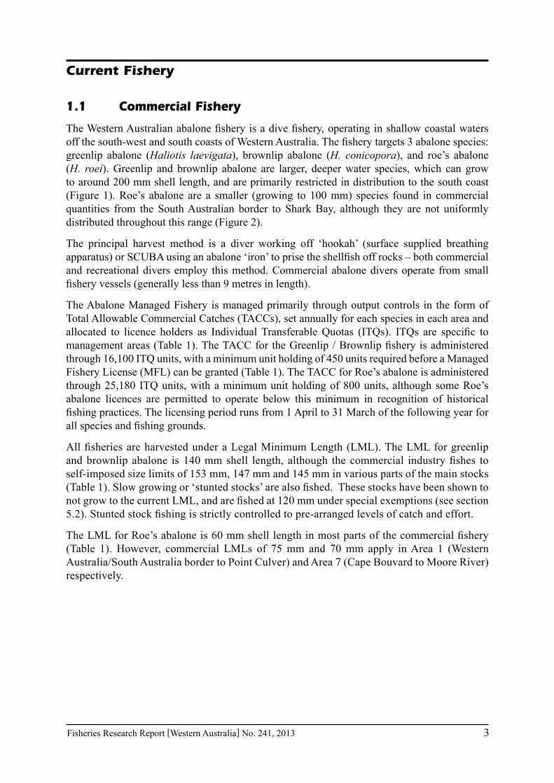
TheWesternAustralianabalonefisheryisadivefishery,operatinginshallowcoastalwatersoffthesouth-westandsouthcoastsofWesternAustralia.Thefisherytargets3abalonespecies:greenlip abalone (Haliotis laevigata), brownlip abalone (H. conicopora), and roe’s abalone (H. roei). Greenlip and brownlip abalone are larger, deeper water species, which can grow to around 200 mm shell length, and are primarily restricted in distribution to the south coast (Figure 1). Roe’s abalone are a smaller (growing to 100 mm) species found in commercial quantities from the South Australian border to Shark Bay, although they are not uniformly distributed throughout this range (Figure 2).
The principal harvest method is a diver working off ‘hookah’ (surface supplied breathing apparatus)orSCUBAusinganabalone‘iron’toprisetheshellfishoffrocks–bothcommercialand recreational divers employ this method. Commercial abalone divers operate from small fisheryvessels(generallylessthan9metresinlength).
The Abalone Managed Fishery is managed primarily through output controls in the form of Total Allowable Commercial Catches (TACCs), set annually for each species in each area and allocated to licence holders as IndividualTransferableQuotas (ITQs). ITQs are specific tomanagementareas(Table1).TheTACCfortheGreenlip/Brownlipfisheryisadministeredthrough 16,100 ITQ units, with a minimum unit holding of 450 units required before a Managed Fishery License (MFL) can be granted (Table 1). The TACC for Roe’s abalone is administered through 25,180 ITQ units, with a minimum unit holding of 800 units, although some Roe’s abalone licences are permitted to operate below this minimum in recognition of historical fishingpractices.Thelicensingperiodrunsfrom1Aprilto31Marchofthefollowingyearforallspeciesandfishinggrounds.
AllfisheriesareharvestedunderaLegalMinimumLength(LML).TheLMLforgreenlipandbrownlip abalone is140mmshell length, although thecommercial industryfishes toself-imposed size limits of 153 mm, 147 mm and 145 mm in various parts of the main stocks (Table1).Slowgrowingor‘stuntedstocks’arealsofished.ThesestockshavebeenshowntonotgrowtothecurrentLML,andarefishedat120mmunderspecialexemptions(seesection5.2).Stuntedstockfishingisstrictlycontrolledtopre-arrangedlevelsofcatchandeffort.
TheLMLforRoe’sabaloneis60mmshelllengthinmostpartsofthecommercialfishery(Table 1). However, commercial LMLs of 75 mm and 70 mm apply in Area 1 (Western Australia/South Australia border to Point Culver) and Area 7 (Cape Bouvard to Moore River) respectively.

4 Fisheries Research Report [Western Australia] No. 241, 2013
Figure 1. Management areas used to set quotas for the commercial greenlip brownlip fishery in Western Australia. Area 4 currently has no quota allocated
Figure 2. Map showing the management areas used to set quotas for the Roe’s abalone commercial fishery in Western Australia.

Fisheries Research Report [Western Australia] No. 241, 2013 5
Table 1. Management details relevant to commercial abalone fisheries in Western Australian. Commercial minimum lengths refer to voluntary minimum lengths imposed by commercial fishers
Species Area
$No. of Fishery
Licenses (MFLs)
#ITQs*Current TACC (t)(2011/12)
*Current value of ITQs (kg)
Legal Minimum Lengths
(mm)
Commercial Minimum
Lengths (mm)
Greenlip 1 6 600 3.2 5.33 120 120
2 6 6000 76.8 12.8 140 145
3 8 7200 93.3 12.96 140 147 & 155
Brownlip 1 6 60 0.06 1.0 140 150
2 6 1440 18.0 12.5 140 150
3 8 800 18.0 22.5 140 150
Roe’s 1 12 1980 5 2.52 60 75
2 12 3600 19.8 5.50 60 75
5 12 4000 20.0 5.00 60 60
6 12 2400 12.0 5.00 60 60
7 12 7200 36.0 5.00 60 70
8 12 6000 0f 0 60 60
TOTAL 315
$ The12MFLsintheRoe’sabalonefisherygenerallyhaveaccessacrossallManagementZones,whereasintheGreenlip/BrownlipfisheryMFLsarerestrictedtoindividualmanagementzones.
# Individual Transferable Quota Units* Whole weight (t) Greenlip and Brownlip TACC. The TACC (and ITQ) are legislated in meat weight, and were
converted to whole weight with a multiplier of 2.667 for Greenlip and 2.5 for Brownlip. f This Area is closed under a Section 43 notice so a TACC of zero is set for this area. See section 7.2.1 for more details.
1.2 Recreational Fishery
Therecreationalabalonefisheryisdividedinto3zones:theNorthernZoneandWestCoastZoneareexclusivelyRoe’sabalonefisheries,whiletheSouthernZoneispredominantlytheGreenlip/Brownliprecreationalfishery,howeverRoe’sabaloneisalsotakeninthisZone(Figure3).Therecreationalfisheryharvestmethodisprimarilywadingandsnorkeling,withthemainfocusofthefisherybeingthePerthmetropolitanstocks(WestCoastFishery),althoughsmalleramountsofgreenlip and brownlip abalone are harvested on compressed air (SCUBA or hookah).
TherecreationalRoe’sabalonefisheryismanagedunderamixofinputandoutputcontrols.Recreational fishers must purchase a dedicated abalone recreational fishing licence. Theselicences are not restricted in number. Total number of licenses currently issued is 18,000 (Figure 4).Historicallyfisherscouldalsopurchasean“umbrella”fishinglicense,underwhichabalonecouldbefished(Figure4),howeverthispracticewasdiscontinuedfrom2010.
ThefishingseasonintheNorthernandSouthernZonesextendsfrom1Octoberto15May.TheWestCoastZoneisonlyopenfor5Sundaysannually,andthetimeoffishingin2006wasreducedfrom90to60minutes(between7a.m.and8.00a.m.),commencingonthefirstSundayinNovember.Asummerfishingseasonwasintroducedin2011withfishingcommencingonthefirstSundayofeach month from November to March These restrictive management controls on the west coast are necessary to ensure the sustainability of an easily accessible (and therefore vulnerable) stock located adjacent to a population in excess of 1.6 million people (including Geraldton).

6 Fisheries Research Report [Western Australia] No. 241, 2013
Thecombineddailybag limit forgreenlipandbrownlipabalone isfiveperfisher(formerly10), and the household possession limit (the maximum number that may be stored at a person’s permanent place of residence) is 20. For Roe’s abalone, the minimum legal size is 60 mm shell length,thedailybaglimitis20perfisher,andthehouseholdpossessionlimitis80.
a)
b)
Figure 3. Maps showing (a) the recreational fishing boundaries for abalone, and (b) the West
Coast (Perth Fishery) zone, showing conservation areas within this zone.

Fisheries Research Report [Western Australia] No. 241, 2013 7
Figure 4. Number of recreational abalone licenses issued during the period 1992 to 2011.
1.3 Illegal Fishery
Quantity of illegal take depends on species. Overall, intelligence operations have revealed that greenlip abalone is the most desirable black market abalone and is easily sold and on sold; roe’s abalone is of limited desirability, with some local black market trade in the Perth metropolitan area, and brownlip abalone is not highly sought and has a very limited black market.
Estimates are that at least 3 tonnes of greenlip abalone per year is taken for the black market on the South Coast. On the West Coast small quantities of excess possession limit metro roes abalone are taken overseas as hand luggage or baggage to Hong Kong, and Singapore.

8 Fisheries Research Report [Western Australia] No. 241, 2013
2.0 Historical development of the fishery
2.1 Catch History
TheabalonefisheryinWesternAustraliaisAustralia’ssmallest,andfishingbeganmoreslowlythan elsewhere because most of the main abalone producing reefs are found in isolated parts of thestate.Theexceptiontothisistheroe’sabalonefisherynearPerth.Fishingofroe’sabalonebegan in 1964, but was minimal and part-time until 1969. Emigration of divers from other states in 1970 resulted in a rapid expansion of catch to maximum of 450 tonnes before dropping back to current levels of between 300 and 350 tonnes (Figure 5a). Total catch has been stable since the early 1970s with an average tonnage around 350 tonnes.
Thegreenlipandbrownlipabalonefisheriesonthesouthcoastarepredominatelycommercialfisheriesandhavebeenthatwaysincetheirinceptionin1970.Greenlipabalonecatchespeakedat270tonnesinthefirstyearofthefishery(1971)andoscillatedbetween150and270tonnesduring the 1970s and 1980s (Figure 5b). Catches dropped rapidly in 1990 to around 150 tonnes and have been at lower levels ever since, averaging around 190 tonnes (Figure 5b). Initially the catch was predominately greenlip, with small by catch of brownlip abalone, however since 1985significantamountsofbrownliphavebeencaughtand it isnowconsideredaseparatefisherywithcatchshowingincreasesinrecentyears(Figure5b).
Asimilarhistoricalpatternisseenintheroe’sabalonefisheries.Commercialcatchesbeganearliestinthisfishery,onthePerthmetropolitanstocksin1964,andthenpeakedat170tonnesin 1971, before declining to a relatively constant level of around 100 tonnes between 1980 and 2010(Figure5c).Recreationalcatchissignificantinthisfishery,currentlycomprisingaround40%ofthetotalcatch(Hartetal.,2010).Recreationalcatchestimatesareavailablesince1992,however considerable recreational catch also occurred in the 1980s. Recent years have seen an increasing recreational catch and total catch of roe’s abalone in currently estimated to be around 160 tonnes (Figure 5c).
Amoredetailedanalysisofcatchandefforttrendsandfinerspatialscalesforindividualspeciesis found in section 11.2.

Fisheries Research Report [Western Australia] No. 241, 2013 9
Figure 5. Historical catch estimates (tonnes whole weight) from abalone fisheries in Western Australia. (A) Total Catch, (B) Greenlip and Brownlip catch – commercial only, (C) Roe’s abalone catch. Historical commercial catches (1964 to 1985) sourced from Prince and Shepherd (1992), and recreational catch (only estimated post 1991) averaged at 30 – 40% of total for roe’s abalone. For greenlip and brownlip, recreational catch is minimal (3 – 4% of total; Hart et. al., 2010), and not included here.

10 Fisheries Research Report [Western Australia] No. 241, 2013
2.2 Management History
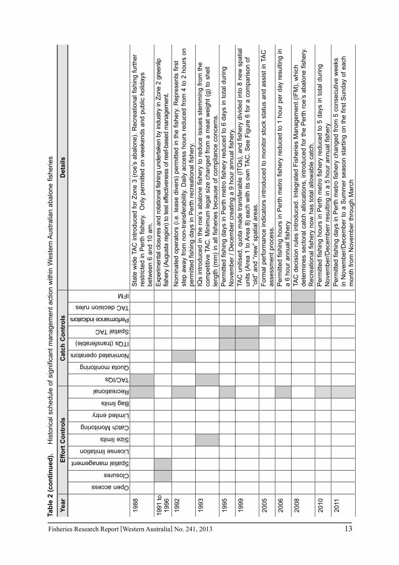
ManagementinWesternAustralianabalonefisherieshasfollowedasimilarevolutionarypathtomanyotherfisheries,beginningwithsimpleeffortcontrols,developingintomorecomplexcatch controls and spatial management.A brief synopsis of the main significant events issummarised inTable2,however thefisheryhasbeenveryadaptiveover its timeandmanychanges have occurred. Only the major developments will be discussed here.
Commercial fishing began in 1964when there were no controls and the fishery was openaccess. By 1971 rapid escalation of catch and license holders prompted the beginning of the firstsetofeffortcontrols,primarilyfocusedonthePerthmetropolitanroe’sabalonefishery.These included the setting of minimum size limits, license limitations and the beginning of spatial management with the use of rolling closures to protect and rest stocks (Table 2). These practices set the scene for the next decade. Formal spatial management was introduced in 1975 withthecreationofthreemanagementzones(Zone1,2and3).Therelationshipbetweenthesezones and the current areas is shown in Figure 6. The new management arrangements were accompanied by catch and effort statistics provided on a monthly basis. The initial licenses were non-transferable and owner-operated, and this was designed to limit any further expansion inthefishery.
DailybaglimitswereintroducedintothePerthcommercialfisheryin1978andremainedfor20 years. Size limits were initially a combination of minimum lengths and minimum meat weight, but by 1993, the emphasis on compliance and ensuring management regulations were enforceable resulted in the adoption of minimum length limits. Changes in size-limits have beenanongoingandregularmanagementpractice in thesefisheries,aswellasfishingareaclosures. For example, theFlindersBaygreenlipbrownlipfishery inZone2 (Area3)wasregularlyclosedandopened,forperiodsofupto2years,between1975and1996.Thisfisheryhas been particularly vulnerable because of its small size and ease of access, and has been intensivelytargetedbyillegalfishingatcertainperiodsinitshistory.
The next evolution in management was the period of catch controls, beginning in 1985 with the setting of a voluntaryTAC (TotalAllowableCatch) in theZone1fishery. TACsweresubsequentlyintroducedtotheZone2fisheryin1986andtheZone3fisheryin1988.Inthegreenlipbrownlipfisheriesthesewereinitiallynon-transferableIQs(IndividualQuotas),setatquite high levels. However, these were not deemed sustainable and TAC dropped substantially in1990inthegreenlipbrownlipfisheries,asevidencebya40%dropincatch(Figure5b).TheTACintheroe’sabalonefishery(Zone3)wasastate-widecompetitivequota,whichcausedafewlocaliseddepletionconcerns,andIQswereeventuallyintroducedintoZone3in1993.
Recreationalfishingcontrolswerefirstintroducedin1980inthePerthroe’sabalonefishery,with a 2 month limited season from October to December. However by 1988 concerns with stock sustainabilityresultedinmorerestrictions;fishingwasonlypermittedonweekendsandpublicholidays,between6and10am.Thisfisheryhassubsequentlyundergonefurtherrestrictions,resultingina9hourannualfisheryin1995,reducedtoa5hourfisheryin2010(Table2).Thefisherynowalsohasatotalallowablerecreationalcatch(TARC),onlythesecondfisheryinWA to be allocated this under the Integrated Fisheries Management (IFM) initiative. Innovative ways to control this TARC are now being considered.
The next major management evolution of the commercial fishery management was theintroduction of transferability, unitisation, and spatial TACs in 1999. These changes were particularly important for the roe’sabalonefishery (theoldZone3fishery).Under thenew

Fisheries Research Report [Western Australia] No. 241, 2013 11
regime,thespatialTACs(6areasintotal)enabledfishingefforttobemoreevenlyspreadacrossthefishery.Significanttradingofquotaunitswereundertakenbetweenlicenseholderswishingtofishinlocalisedareasclosetohome.
Development of performance indicators and formal decision rules to assess annual TACs was introduced over the period 2005 – 2009 and these now underlie the main management functions relating to setting of a sustainable catch.

12 Fisheries Research Report [Western Australia] No. 241, 2013
Tab
le 2
.
His
toric
al s
ched
ule
of s
igni
fican
t m
anag
emen
t ac
tion
with
in W
este
rn A
ustr
alia
n ab
alon
e fis
herie
s
Yea
rE
ffo
rt C
on
tro
lsC
atch
Co
ntr
ols
Det
ails
Open access
Closures
Spatial management
License limitation
Size limits
Catch Monitoring
Limited entry
Bag limits
Recreational
TAC/IQs
Quota monitoring
Nominated operators
ITQs (transferable)
Spatial TAC
Performance indicators
TAC decision rules
IFM
1964
Initi
al f
ishi
ng in
Per
th r
oe’s
aba
lone
fis
hery
. O
pen
acce
ss.
1971
Lice
nse
limita
tion
intr
oduc
ed.
36 n
on-t
rans
fera
ble
com
mer
cial
lice
nses
, re
duce
d to
25
by 1
975.
Rol
ling
clos
ures
beg
in in
Per
th f
ishe
ry o
n ap
prox
. a
3 ye
ar r
otat
ion
betw
een
Nor
th,
Cen
tral
, an
d S
outh
are
as.
Sys
tem
con
tinue
s til
l 198
2. S
ize
limits
(6
0 m
m)
intr
oduc
ed in
roe
’s a
balo
ne f
ishe
ry.
1972
Min
imum
siz
e lim
it (1
00 m
m)
intr
oduc
ed f
or g
reen
lip a
nd b
row
nlip
fis
hery
, co
rres
pond
ing
to s
ize
at m
atur
ity.
1975
For
mal
spa
tial m
anag
emen
t in
trod
uced
. T
hree
zon
es c
reat
ed.
Zon
e 1
(6 d
iver
s)
and
Zon
e 2
(8 d
iver
s) f
or t
he g
reen
lip a
nd b
row
nlip
fis
hery
. Z
one
3 (1
2 di
vers
) fo
r th
e ro
e’s
abal
one
fishe
ry.
Siz
e lim
its f
or g
reen
lip a
nd b
row
nlip
fis
herie
s ch
ange
d to
m
inim
um w
eigh
t of
113
g.
Mon
thly
cat
ch a
nd e
ffort
mon
itorin
g (C
AE
S)
intr
oduc
ed
at t
he s
patia
l sca
le o
f 1
degr
ee (
60 x
60
naut
ical
mile
s).
Flin
ders
Bay
(Z
one
2)
gree
nlip
fis
hery
clo
sed
for
2 ye
ars
1976
Lim
ited
entry
(ow
ner
oper
ated
, non
-tran
sfer
able
lice
nses
) fir
st in
trodu
ced
in Z
one
2.
1978
Dai
ly b
ag li
mit
(100
kg)
intr
oduc
ed f
or P
erth
com
mer
cial
fis
hery
. R
emai
ns in
pla
ce
till 1
999
whe
n th
e 36
ton
ne s
patia
l TA
C in
trod
uced
. F
linde
rs B
ay (
Zon
e 2)
gre
enlip
fis
hery
clo
sed
for
18 m
onth
s
1980
Siz
e lim
its in
Per
th f
ishe
ry in
crea
sed
from
60
to 7
0 m
m.
Flin
ders
Bay
(Z
one
2) g
reen
lip f
ishe
ry c
lose
d fo
r 2
year
s. R
ecre
atio
nal f
ishe
ry in
Per
th li
mite
d to
a
seas
onal
ope
ning
fro
m m
id-O
ctob
er t
o m
id-D
ecem
ber.
1985
Tota
l Allo
wab
le C
atch
(TA
C)
intr
oduc
ed t
o Z
one
1. T
AC
initi
ally
allo
cate
d as
no
n-tr
ansf
erab
le I
Q (
Indi
vidu
al Q
uota
). S
ize
limit
in g
reel
ip a
nd b
row
nlip
fis
hery
in
crea
sed.
1986
TAC
intr
oduc
ed t
o Z
one
2. F
linde
rs B
ay (
Zon
e 2)
gre
enlip
fis
hery
clo
sed
for
2 ye
ars.
Spa
tially
del
imite
d si
ze li
mits
intr
oduc
ed t
o Z
one
2.
Dai
ly c
atch
(qu
ota)
and
ef
fort
mon
itorin
g in
trod
uced
, in
itial
ly in
Zon
e 2.
Fisheries Research Report [Western Australia] No. 241, 2013 13
Tab
le 2
(co
nti
nu
ed).
H
isto
rical
sch
edul
e of
sig
nific
ant
man
agem
ent
actio
n w
ithin
Wes
tern
Aus
tral
ian
abal
one
fishe
ries
Yea
rE
ffo
rt C
on
tro
lsC
atch
Co
ntr
ols
Det
ails
Open access
Closures
Spatial management
License limitation
Size limits
Catch Monitoring
Limited entry
Bag limits
Recreational
TAC/IQs
Quota monitoring
Nominated operators
ITQs (transferable)
Spatial TAC
Performance indicators
TAC decision rules
IFM
1988
Sta
te w
ide
TAC
intr
oduc
ed f
or Z
one
3 (r
oe’s
aba
lone
). R
ecre
atio
nal f
ishi
ng f
urth
er
rest
ricte
d in
Per
th f
ishe
ry.
Onl
y pe
rmitt
ed o
n w
eeke
nds
and
publ
ic h
olid
ays
betw
een
6 an
d 10
am
.
1991
to
1996
Exp
erim
enta
l clo
sure
s an
d ro
tatio
nal f
ishi
ng u
nder
take
n by
indu
stry
in Z
one
2 gr
eenl
ip
fishe
ry (
Aug
usta
reg
ion)
to te
st e
ffect
iven
ess
of r
eef-b
ased
man
agem
ent.
1992
Nom
inat
ed o
pera
tors
(i.e
. le
ase
dive
rs)
perm
itted
in t
he f
ishe
ry.
Rep
rese
nts
first
st
ep a
way
fro
m n
on-t
rans
fera
bilit
y. D
aily
acc
ess
hour
s re
duce
d fr
om 4
to
2 ho
urs
on
perm
itted
fis
hing
day
s in
Per
th r
ecre
atio
nal f
ishe
ry.
1993
IQs
intr
oduc
ed in
the
roe
’s a
balo
ne f
ishe
ry t
o re
duce
issu
es s
tem
min
g fr
om t
he
com
petit
ive
TAC
. M
inim
um le
gal s
ize
chan
ged
from
a m
eat
wei
ght
(g)
to s
hell
leng
th (
mm
) in
all
fishe
ries
beca
use
of c
ompl
ianc
e co
ncer
ns.
1995
Per
mitt
ed f
ishi
ng d
ays
in P
erth
met
ro f
ishe
ry r
educ
ed t
o 6
days
in t
otal
dur
ing
Nov
embe
r /
Dec
embe
r cr
eatin
g a
9 ho
ur a
nnua
l fis
hery
.
1999
TAC
uni
tised
, qu
ota
mad
e tr
ansf
erab
le (
ITQ
s),
and
fishe
ry d
ivid
ed in
to 8
new
spa
tial
units
(A
rea
1 to
Are
a 8)
eac
h w
ith it
s ow
n TA
C.
See
Fig
ure
6 fo
r a
com
paris
on o
f “o
ld”
and
“new
” sp
atia
l are
as.
2005
For
mal
per
form
ance
indi
cato
rs in
trod
uced
to
mon
itor
stoc
k st
atus
and
ass
ist
in T
AC
as
sess
men
t pr
oces
s.
2006
Per
mitt
ed f
ishi
ng h
ours
in P
erth
met
ro f
ishe
ry r
educ
ed t
o 1
hour
per
day
res
ultin
g in
a
6 ho
ur a
nnua
l fis
hery
2008
TAC
dec
isio
n ru
les
intr
oduc
ed.
Inte
grat
ed F
ishe
ries
Man
agem
ent
(IF
M),
whi
ch
dete
rmin
es s
ecto
ral c
atch
allo
catio
ns,
intr
oduc
ed f
or t
he P
erth
roe
’s a
balo
ne f
ishe
ry.
Rec
reat
iona
l fis
hery
now
has
tot
al a
llow
able
cat
ch.
2010
Per
mitt
ed f
ishi
ng h
ours
in P
erth
met
ro f
ishe
ry r
educ
ed t
o 5
days
in t
otal
dur
ing
Nov
embe
r/D
ecem
berr
res
ultin
g in
a 5
hou
r an
nual
fis
hery
2011
Per
mitt
ed f
ishi
ng d
ays
in P
erth
met
ro f
ishe
ry c
hang
ed f
rom
5 c
onse
cutiv
e w
eeks
in
Nov
embe
r/D
ecem
ber
to a
Sum
mer
sea
son
star
ting
on t
he f
irst
Sun
day
of e
ach
mon
th f
rom
Nov
embe
r th
roug
h M
arch

14 Fisheries Research Report [Western Australia] No. 241, 2013
Figure 6. General map comparing old zonal arrangements (1975-1998; Zone 1, 2 & 3) and new area management areas (1999-2012+) of the commercial abalone fisheries of
Western Australia

Fisheries Research Report [Western Australia] No. 241, 2013 15
3.0 Abalone biology and life history parameters
Abalone are marine archaeogastropods (snails) with a worldwide distribution in tropical and temperate waters (Lindberg, 1992). All commercially targeted Western Australian species of abalone live on exposed, high-energy coasts and have evolved life-history characteristics to enable survival in this environment. General traits include: a muscular foot capable of providing solid attachment during periods of prolonged exposure; a feeding behaviour primarily focused on drifting algae dislodged by wave action, rather than actively grazing as do many other gastropods herbivores (Shepherd and Steinberg, 1992); broadcast spawning by separate sexes, synchronised by seasonal cue’s such as change in water temperature and lunar periods, and a relatively short larval life-span of between 5 and 10 days to allow for quick settlement back into localised populations (McShane, 1992); use of specialised larval settlement substrate such as crustose coralline algae, and a relatively slow and long-lived life duration (McShane, 1992).
Managing harvest of these species requires detailed knowledge of the specific biology andhabitat such as growth and mortality rates, length-weight relationships, and reproductive characteristics such as size-at-maturity and fecundity.
3.1 Greenlip abalone (Haliotis laevigata)
3.1.1 Growth
GrowthofgreenlipabaloneinWesternAustraliavariessignificantlybetweenpopulations.Atthe faster end, greenlip abalone populations reach an average maximum size of 175 mm (Table 3). At the lower end of the growth spectrum, stunted stocks show an average maximum size of 125 – 133 mm shell length, which is below the legal minimum length (Table 3). This is a difference in growth of between 12 and 38 mm yr-1 for an 80 mm animal in different areas.
Allabaloneexhibitlargespatialheterogeneityingrowth,with“stunted”populationsoccurringinallabalonefisheries(WellsandMulvay,1995).Toensureoptimalandsustainableexploitation,populations with different growth characteristics require harvest strategies that account for this variability. Typically this is achieved via the use of spatially varying size-limits and TACCs matched to the productivity of the population (Mayfield and Saunders, 2008; Prince et al.,2008,TarbathandOfficer,2003). In thecaseofHaliotis laevigata, comparisons of growth parameters from tag-recapture studies across Australia reveal a wide variability within and betweenfisheries(Figure7).

16 Fisheries Research Report [Western Australia] No. 241, 2013
Figure 7. Von Bertalanffy growth parameters (K, L∝) from Haliotis laevigata populations within and between state fisheries in Australia. Data have been grouped into “stunted”, “normal” and “fast” growth stocks in relation to the LML of 140 mmm (dashed line) for the Western Australian fishery. Growth parameters sourced from: this report (Table 3), Mayfield et al., (2003), Officer (1999), Shepherd and Hearn (1983), Shepherd et al. (1992), Wells and Mulvay (1995).
3.1.2 Natural mortality
Natural mortality (M) in adult greenlip abalone has been estimated between 0.15 and 0.4, dependingonmethodandlocation(Table3).ForthemostpartMisassumedtobe0.25(22%perannum)forWA’scommerciallyfishedpopulation.
To obtain an estimate of fishingmortality from length-frequency data, growth assumptionswere made to represent the entire stock in different areas (Table 3). These growth parameters provided the best fit for length-converted catch-curve estimates of Z and are a reasonablerepresentation of average growth for the overall population. See section 5.1.5.

Fisheries Research Report [Western Australia] No. 241, 2013 17
Table 3. Natural mortality and growth information for Haliotis laevigata from Western Australia. Growth is estimated from tag-recapture data and growth assumptions are made for model estimates of fishing mortality based on length-converted catch curves (see section 5.1.5) and yield-per-recruit analysis (see section 5.5).
LocationNatural
Mortality (M)
Growth parameters (von
Bertalannfy)*
Growth rate (mm.y-1) for an 80 mm
animal
Source
K L∝ (±SD)
All 0.25 Unpublished data
South Australia 0.15 – 0.40 Mayfield et al. (2003)
Growth estimates from tag-recapture
Augusta (Outback) 0.55 170 (14) 38 Hart et al. (1999)
Augusta (Flinders Bay) 0.36 165 (10) 34 Wells and Mulvay (1995)
Hopetoun (2 Mile Main stocks)
0.33 145 (14) 29 Unpublished data
Hopetoun (2 Mile stunted stocks)
0.34 133 (13) 12 Unpublished data
Station Island (Duke of Orleans Bay) – stunted
0.60 128 (12) 22 Unpublished data
Pt Malcolm (Israelite Bay) – stunted
0.55 124 (9) 18 Unpublished data
Growth parameters for length-converted catch curve and yield-per-recruit analysis
West Coast (Augusta) 0.30 185 27
South Coast (Area 3) 0.25 179 22
Area 2 0.25 179 22
* Growth parameters estimated using maximum likelihood (see Francis, 1988)
3.1.3 Length-weight relationships
Length-weight relationships for greenlip abalone in Western Australia are summarised in Figure 8. Relationships vary slightly between areas, for example a 160 mm animal at Flinders Bay, Augusta has an average meat weight of 230 g, compared to 186 g for the same-sized animal at Windy Harbour (Figure 8).

18 Fisheries Research Report [Western Australia] No. 241, 2013
(A)
40 60 80 100 120 140 160 180
Wei
gh
t (g
)
0
100
200
300
400
500
600
700
800
900
1000whole weightmeat weight
a = 5x10⁻⁵
b = 3.211
a = 7 x 10⁻⁶
b = 3.402
(B)
40 60 80 100 120 140 160 180
0
100
200
300
400
500
600
700
800
900
1000
a = 3x10⁻⁵
b = 3.343
a = 9 x 10⁻⁶
b = 3.363
(C)
40 60 80 100 120 140 160 180
Wei
gh
t (g
)
0
100
200
300
400
500
600
700
800
900
1000
a = 5x10⁻⁵
b = 3.213
a = 1 x 10⁻⁵
b = 3.298
(D)
40 60 80 100 120 140 160 180
0
100
200
300
400
500
600
700
800
900
1000
a = 4x10⁻⁵
b = 3.281
a = 5 x 10⁻⁶
b = 3.452
(E)
Length (mm)
40 60 80 100 120 140 160 180
Wei
gh
t (g
)
0
100
200
300
400
500
600
700
800
900
1000
a = 2x10⁻⁵
b = 3.47
a = 3 x 10⁻⁶
b = 3.61
(F)
Length (mm)
40 60 80 100 120 140 160 180
0
50
100
150
200
250
300
350
400
(A)(B)(C)(D)(E)
Figure 8. Length-whole weight (blue line), and length-meat weight (red line) relationships for Haliotis laevigata at 5 sites in Western Australia: A) Augusta (outback); B) Augusta (Flinders Bay); C) Windy Harbour; D) Hopetoun; E) Point Malcolm, F) comparison of length – meat weight relationships between areas. The equation is W=aLb

Fisheries Research Report [Western Australia] No. 241, 2013 19
3.1.4 Size-at-maturity and length-fecundity
Size-at-maturity and length-fecundity relationships for greenlip abalone in Western Australia are summarised in Table 4. Average size-at-maturity for females varies between 78 and 97 mm (Table 4), and appears to be primarily dependent on growth rate. Based on growth data, age-at-maturity is expected to be about 3 years, although there is some evidence that maturation is not entirely age dependent, and can be accelerated under optimal conditions (McAvaney et al., 2004). However there are generally at least 2 breeding years protected by the LML of 140 mm.
Table 4. Size-at-maturity and length-fecundity relationships for Haliotis laevigata at 6 sites in Western Australia. Length-fecundity equations are of the form F =aLb, where F is
fecundity (millions of eggs), and L is length (mm)
LocationSize at
50% maturity (mm)
Length-Fecundity parameters Source
a b
Augusta (fast) 97 1.00 × 10⁻⁶ 5.48 Hart et al. (2000)
Augusta (normal) 87 1.49 × 10⁻³ 4.29 Wells and Mulvay (1992)
Augusta (stunted) 78 1.39 × 10⁻⁴ 4.70 Wells and Mulvay (1992)
Hopetoun (normal) 6.91 × 10⁻⁴ 4.42 Wells and Mulvay (1992)
Hopetoun (stunted) 81 Wells and Mulvay (1992)
Cape Arid (normal) 88 4.95 × 10⁻⁵ 4.99 Wells and Mulvay (1992)
Cape Arid (stunted) 85 6.19 × 10⁻⁴ 4.42 Wells and Mulvay (1992)
3.2 Roe’s abalone (Haliotis roei)
3.2.1 Growth and natural mortality
Estimates of natural mortality (M) of adult roe’s abalone vary between 0.13 and 0.17, or between 12and16%perannum(Table5).
Growthofroe’sabalonevariessignificantlybetweenpopulations.At thehigherrange,roe’sabalone reach an average maximum size of 89 mm (Table 5). At the lower end of the growth spectrum, slow growing stocks show an average maximum size of 73 – 75 mm shell length (Table 5). This is a difference in growth of between 6 and 14 mm yr-1 for a 40 mm animal.
To obtain an estimate of fishingmortality from length-frequency data, growth assumptionswere made to represent the entire stocks in different areas (Table 5). These growth parameters provided the best fit for length-converted catch-curve estimates of Z and are a reasonablerepresentation of average growth for the overall population.
3.2.2 Length-weight relationships
Length-weight relationships for roe’s abalone in Western Australia are summarised in Figure 9.
3.2.3 Size-at-maturity and length-fecundity relationships
Size-at-maturity and length-fecundity relationships for roe’s abalone in Western Australia are summarised in Table 6. Size–at-maturity for females is around 40 mm shell length. Based on growth data, age-at-maturity is expected to be about 3 years, similar to greenlip and brownlip abalone. There are generally one or two breeding years protected by the LML of 60 mm.

20 Fisheries Research Report [Western Australia] No. 241, 2013
Table 5. Natural mortality and growth information for Haliotis roei from Western Australia. Growth is estimated from tag-recapture data and growth assumptions are made for model estimates of fishing mortality based on length-converted catch curves (see section 4.4.2.2)
LocationNatural
Mortality (M)
Growth parameters (von Bertalannfy)
Growth rate (mm.y-1) for a 40 mm animal
Source
K L∝
All 0.13 – 0.16 Unpublished data
Growth estimates from tag-recapture
Waterman’s Reserve (North platform)
0.31 89 13 Hancock (2004)
Waterman’s Reserve (North subtidal)
0.40 83 14 Hancock (2004)
Waterman’s Reserve (South platform)
0.44 81 14 Hancock (2004)
Waterman’s Reserve (South subtidal)
0.34 86 13 Hancock (2004)
Shag Rock (Trigg Island)
0.42 73 12 Hancock (2004)
Three Bears (Margaret River)
0.20 75 6 Hancock (2004)
Bald Face (Kalbarri) 0.35 73 10 Hancock (2004)
Growth assumptions for length converted catch – curve analysis
Gompertz parameters g L∝ t0
Area 7 (Perth Metro) 0.57 88 2.2 16
Area 6 0.45 83 2.2 13
Area 7 (Perth Metro) 0.57 88 2.2 16

Fisheries Research Report [Western Australia] No. 241, 2013 21
(A)
20 30 40 50 60 70 80 90 100
Wei
gh
t (g
)
0
20
40
60
80
100
120
140
160
180 whole weightmeat weight a = 2 x10⁻⁴
b = 3.002
(B)
Length (mm)
20 30 40 50 60 70 80 90 100
Wei
gh
t (g
)
0
20
40
60
80
100
120
140
160
180
a = 7 x 10⁻⁵
b = 3.06
a = 3x10⁻⁴
b = 2.86
a = 5 x 10⁻⁵
b = 3.07
Figure 9. Length-whole weight (blue line), and length-meat weight (red line) relationships for Haliotis roei at 2 sites in Western Australia: A) Perth metro (Area 7), B) Cape Naturaliste – Cape Leeuwin (Area 6). The equation is W=aLb

22 Fisheries Research Report [Western Australia] No. 241, 2013
Table 6. Size-at-maturity and length-fecundity relationships for Haliotis roei at 2 sites in Western Australia. Length-fecundity equations are of the form F =aLb, where F is fecundity (millions of eggs), and L is length (mm)
LocationSize at 50%
maturity (mm)
Length-Fecundity parameters Source
a b
Perth (Waterman) 40 1.98 × 10⁻² 4.52 Keesing (1984)
Perth (Marmion)* 9.00 × 10⁻⁸ 4.28 Unpublished data
* the fecundity parameters (a,b) for Marmion are for length-gonad weight equations of the form GW =aLb, where GW is gonad weight (g).
3.3 Brownlip abalone (Haliotis conicopora)
3.3.1 Growth and natural mortality
Studies of natural mortality (M) of adult brownlip abalone in Western Australia have not been undertaken to date. M was assumed to be 0.25, based on data from blacklip abalone (Haliotis rubra)intheWesternZoneofSouthAustralia(Table7).
Estimates of von Bertalanffy growth parameters from tag-recapture studies for brownlip abalone areprovidedinTable7.Toobtainanestimateoffishingmortalityfromlength-frequencydata,growthparametersfromHopetounOldfieldsstocks(L∞ = 198 mm and K = 0.32) were applied (Table 7). These growth parameters provided the best fit for length-converted catch-curveestimatesofZandareareasonablerepresentationofaveragegrowthfortheallpopulations.
Table 7. Natural mortality and growth information for Haliotis conicopora from Western Australia. Growth is estimated from tag-recapture data and growth assumptions are made for model estimates of fishing mortality based on length-converted catch curves (see section 5.1.5) and yield-per-recruit analysis (see section 5.5).
LocationNatural Mortality
(M)
Growth parameters (Von Bertalannfy) SourceK L∝ (mm)
All 0.25 (3+ animals) Mayfield et al., (2003)
Growth estimates from tag-recapture
Hopetoun Masons 0.32 (± 0.03) 183 (± 2.5) Unpublished data
Hopetoun Oldfields 0.32 (± 0.05) 198 (± 6.3) Unpublished data
Growth parameters (assumptions) for length converted catch – curve analysis
All Stocks 0.32 198
3.3.2 Length-weight relationships
Length-weight relationships for brownlip abalone in Western Australia are only preliminary estimates due to lack of information of smaller sized animal’s. The equations for Cape Leeuwin are summarised in Figure 10.

Fisheries Research Report [Western Australia] No. 241, 2013 23
(B)
Length (mm)
40 60 80 100 120 140 160 180 200
Wei
gh
t (g
)
0
200
400
600
800
1000
1200
1400a = 2 x10⁻⁴
b = 2.995
a = 8 x 10⁻⁵
b = 2.93
Figure 10. Length-whole weight (blue line), and length-meat weight (red line) relationships for
Haliotis conicopora at Cape Leeuwin in Western Australia. The equation is W=aLb.
3.3.3 Size-at-maturity and length-fecundity relationships
Size-at-maturity and length-fecundity relationships for brownlip abalone in Western Australia are summarised in Table 8. Size–at-maturity for females is around 120 – 125 mm shell length. Age-at-maturity is expected to be about 3 years, similar to greenlip and roe’s abalone.
Table 8. Size-at-maturity and length-fecundity relationships for Haliotis conicopora at 2 sites in Western Australia. Length-fecundity equations are of the form F =aLb, where F is fecundity (millions of eggs), and L is length (mm)
LocationSize at 50%
maturity (mm)
Length-Fecundity parameters Source
a b
Augusta (Area 3) 125 1.34 × 10⁻² 3.74 Wells and Mulvay (1992)
Cape Arid (Area 2) 120 1.69 × 10⁻³ 4.15 Wells and Mulvay (1992)

24 Fisheries Research Report [Western Australia] No. 241, 2013
4.0 Research and assessment methodology
4.1 Commercial fisheries data collection
4.1.1 Monthly catch and effort logbooks (1975+)
Catch and effort information was collected on a monthly basis by divers submitting compulsory monthly catch returns to the Research Divisions CAES (Catch And Effort System). This system encompassesallfisheriesinWAandthedataisdividedupintolargegridsystems(60x60mile).Although it is not as detailed as the ACE (Abalone Catch and Effort) database, catch data has been entered in this system since the late 1970’s, and it is a useful source of archival information.
4.1.2 Daily catch and effort logbooks
For eachday’sfishing, commercialdivers recordestimatesof catch (kg), effort (hours) spentdivingforabalone,andlocationfishedwithina10x10milegridsystem(Section11.2).Thedatais stored on a daily Catch and Disposal Record (CDR) that accompanies each daily catch, which is officiallyweighedatalicensedprocessors,andenteredintotheACE(AbaloneCatchandEffort)effortdatabaseatRegionalFisheryOffices.Inthegreenlipandbrownlipfisheries,thenumberofabalonecaughtisrecorded,enablingestimatesofmeanweightofabalonefromeachday’sfishing.
4.2 Recreational fisheries data collection
Currentannualrecreationalcatchandeffortestimatesarederivedfromanannualfieldsurvey(West Coast Zone / Perth metropolitan fishery), and an occasional telephone diary surveycovering the entire state. The last year of the telephone diary survey was in 2007.
4.2.1 Field surveys – Perth metropolitan roe’s abalone fishery
Thefieldsurveyestimatesthecatchandeffortfromeachdistinctroe’sabalonestockwithinthePerthfishery,andestimatesarebasedonaveragecatch(weightandnumbers),catchrates(derivedfrom1,000interviewsin2007),andfishercountsconductedbyFisheriesVolunteersand research personnel from shoreline vantage points and aerial surveys (Hancock and Caputi, 2006).Thismethodprovidesacomprehensiveassessmentofthe5-daymetropolitanareafishery,but is too resource-intensive to be applied routinely outside of the Perth metropolitan area.
4.2.2 Weather conditions, license numbers and recreational abalone catch
Due to theconstrainednatureof thePerth recreational roe’sabalonefishery (1hourperday;5 hours per annum), weather conditions are hypothesised to play a major role in determining thetotalamountcaught.Aweatherconditionindexwasdevelopedforthefishery(HancockandCaputi, 2006), however has not previously been used to investigate the annual variability in catch.
As a preliminary analysis, the daily weather condition indexwas quantified for each daysfishing(n=5),andtheannualindexwasthemeanofthese.Theeffortinhoursfishedwasalsoestimated, based on methodology described by Hancock and Caputi (2006).
Annual catch estimates were modelled with a multiple regression model incorporating the explanatory variables of weather condition index in year i (Wi),andeffort(hoursfished)inyeari (Ei). The estimation model was as follows

Fisheries Research Report [Western Australia] No. 241, 2013 25
logCatchi = aWi + blogEi + c + εi
where aisthepartialregressioncoefficientforWi, bisthepartialregressioncoefficientforEi, c is the the intercept and ε~N(0,θ2).
4.2.3 Phone diary surveys – entire state
The telephone diary survey estimates the catch of all three species on a state-wide basis. In 2007, around 500 licence holders were randomly selected from the licensing database, with selectionstratifiedbylicencetype(abaloneorumbrella)andrespondentlocation(countryorPerthmetropolitanarea).Thelicenceholdersweresentadiarytorecordtheirfishingactivityand were contacted every 3 months by telephone for the duration of the abalone season, or at the end of the season for those only involved in the Perth abalone season.
4.3 Fishery independent stock surveys
4.3.1 Research diver transect surveys
4.3.1.1 Greenlip and Brownlip abalone
A survey method developed for Haliotis rubra (Gorfineet al., 1998;Hart et al., 1997)wasadapted for greenlip and brownlip abalone in Western Australia. Method development occurred over2003to2005.Themethodinvolvesrepeatedsurveysatfixedsitesrepresentingallareasofthefishery.Surveysiteswereselectedonthebasisofknownstockdistributionsandcurrentlythereare85stocksurveysitesintheArea2fisheryand116intheArea3fishery,targetingarange of sites of different productivity (Table 9). The Arid and Augusta sub-areas are surveyed annually, and other sub-areas visited every 2 – 3 years. Another 28 sites have been surveyed and used for stock enhancement experiments (Hart et al., in press a, Hart et al., in press b), and a further 150 sites have been set up as baseline survey sites to examine the effects of proposed marine parks (Table 9). Further details for abalone surveys in proposed marine parks are found in Hesp et al., (2008).
Table 9. Fishery-independent survey sites in the greenlip and brownlip fishery.
Management Area
Sub-AreaStock survey
sitesStock
enhancement sitesCapes-Capes
Marine Park sites
2
Arid 27
Duke 12
Israelite 12
Town 16
West 18
3
Albany 28
Augusta 29 28 150
Hopetoun 44
Windy Harbour 15
TOTAL 202 28 150 380
At each site, 2 or 3 survey transects of 30 m2 (30 x 1 m) divided into 1 m2 quadrats are surveyed. Observers swim out a rope marked at 1m intervals and measure the abundance and size of greenlip and brownlip abalone within each 1m2 quadrat. The area of suitable abalone

26 Fisheries Research Report [Western Australia] No. 241, 2013
habitat is also quantified according to criteria developed in Table 10 and utilised to obtain a density estimate. Suitable abalone habitat was defined as habitable surfaces (generally granite or limestone) of sufficient quality and area to allow effective attachment for abalone above 40mm shell length (1+ years). Younger juveniles are cryptic, while the larvae settle preferentially on non-geniculate coralline algae, and require different habitat and sampling requirements (Daume et al., 1999; McShane, 1995). Density estimates were obtained with the following equation:
Density = # abalone / m2 of habitat.
Table 10. Habitat survey criteria for Haliotis laevigata. Codes are applied to each 1m2 quadrat within the larger sample unit (a 30m2 transect). An estimate of the total area of habitat per 30m2 transect is obtained by summing the midpoints for each quadrat.
Code Habitat Area (m2) Midpoint (m2)
0 0 0
1 0 – 0.1 0.05
2 0.1 – 0.2 0.15
3 0.2 – 0.3 0.25
4 0.3 – 0.5 0.4
5 0.5 – 1.0 0.75
6 >1.0 1.1
Density in Haliotis laevigataisanalysedbyfiveageclassesforbothstuntedandprimarystocks(Table 11). These correspond to approximate year classes prior to recruitment, plus recruited animals. Note that the size classes considered as recruit animals (147 mm+) in the primary stocksarehigherthanthelegalminimumlengthof140mm,becausetheyarefirstcommerciallyharvested at these larger size classes. In the stunted stocks size classes considered as recruits are less than the LML because of much slower growth (see section 5.2).
Estimates of density trends for each sub area (Figure 12; Figure 13) were derived using a 3-factor (Year,Site,Diver)ANOVAmodel.Theanalysiswascarriedout inS_Plus®. A logarithmic transformation of raw data was undertaken to take into account the skewed distribution associated with density. The least squares mean of the factor Year was used to produce an index of density, standardised by site and diver, for each year.
Table 11. Size (mm) and age classes used in the analysis of greenlip abalone survey density.
Size class (Primary stocks)
Size class (Stunted stocks)
Age-class (approximate)
Description
< 90 mm (juveniles)
< 80 mm (juveniles)
1 – 3 years Juvenile animals, not part of the breeding stocks
90 – 114 80 – 104 3+ Approximately 3 years of age, about 3 years prior
to recruitment into the Recruits size-class
115 – 134 105 – 119 4+Approximately 4 years of age, about 2 years prior
to recruitment into the Recruits size-class
135 – 146 120 – 129 5+ Approximately 5 years of age, about 1 years prior
to recruitment into the Recruits size-class
≥147 ≥130 RecruitsApproximately 6+ years of age – animals recruited
into the exploited population.

Fisheries Research Report [Western Australia] No. 241, 2013 27
4.3.1.2 Roe’s abalone
Size anddensity of roe’s abalone in thePerthmetropolitanfishery ismeasured annually at13indicatorsitesbetweenYanchepandPenguinIsland.Elevenofthesearefishedwhiletheother two are the Waterman’s Reserve Marine Protected Area (MPA) and the Cottesloe Fish HabitatProtectionZone.Sitesinitiallybeganin1996at5sites,withthefullcomplementof13indicator sites available from 2011 onwards.
Surveys are carried out on two habitats, the reef platform and the sub-tidal habitat, which generallycorrespondtotherecreationalandcommercialfisheriesrespectively.Themethodologyinvolvessurveyingfixedquadratsof0.25and0.5m2 at each site and counting and measuring all animals within these quadrats (Figure 11). For further details of survey methodology, see Hancock (2004).
Estimatesofdensitywerederivedusinga3-factor(Year,Location,Habitat)ANOVAmodel.TheanalysiswascarriedoutinS_Plus®. A logarithmic transformation of raw data was undertaken to take into account the skewed distribution associated with density. The least squares mean of the factor Year was used to produce an index of density, standardised by location and habitat, for each year.
Figure 11. Research diver undertaking surveys for Haliotis roei in shallow water. The yellow
vest contains an extra 15 kg of weight to counteract the swell.
Preliminary investigations on the predictive capacity of pre-recruit density estimates were also undertaken. Data on Age 1+ abundance (17 – 32 mm) were taken from the outer and middle platform habitats, and Age 5+ data (71 mm) was from all habitats. Regression analysis was applied using a 4-year lag between the juvenile and adult age classes.
4.3.2 Digital video surveys
Size and density of greenlip abalone are surveyed by commercial industry divers using a specificallydevelopedvideosurveymethodologyfor thesespecies(Hartetal.,2008.). Thereasonforusingindustrydiversisacost-effectivemeasureasmanyfishingsitesareremote.

28 Fisheries Research Report [Western Australia] No. 241, 2013
ThemethodisbeingusedprimarilyintheArea2greenlipabalonefishery.Intheperiod2008to 2012, between 26 and 82 sites were surveyed per year by an industry diver using a random survey method.
Thesurveydesignisasfollows.TheArea2fisheryisdividedupintothe4mainsub-areas,described in Figure 12, and a minium sample size of 10 sites is required for each area, up to amaximumof30.Whilstfishing inanygivensub-area thecommercialdiverfilmsonesiteper day, at the commencement of the 2nd dive, prior to harvesting the animals. This ensures a randomised site selection process. The procedure is to undertake a 10-minute (approx.) survey, filming each abalone in turn so that lengths for each animal can be later determined. Thefootage is sent back to the Research Division, where the images are extracted and counts of abalone density and estimates of length are undertaken using digital image analysis software. Full details of the methodology are summarised in Hart et al. (2008).
For each site, a total count of abalone is made over the timed survey (usually 9 – 12 minutes), and 30%ofanimalswithsufficientimagequalityarerandomlyselectedforlengthmeasurements.In sites where abundance is low, a minimum selection of 20 animals is made per site to enable a representative sample.
Shell length (in mm) is used to estimate mean length and population length-frequency. These datacanalsobeusedtoestimatefishingmortalityaspermethodsdescribedinsection4.4.2.For abundance estimates, the length data is separated into approximate age groups described in Table 11. Abundance is estimated as number per minute searched. The time spent searching is totaltimeminusfilmingandscootingtime.Diversuseamechanisedscootertomovebetweendiscretehabitatsclusters,andthiscanbesubstantialpartofthefilmingtimethatneedstobeaccounted for (see Hart et. al., 2008 for details).
4.4 Data analysis and stock assessment
4.4.1 Standardised catch per unit effort
Catch and effort data are analysed at pertinent spatial and temporal scales. Stock indicator variables include catch, effort, daily catch rate (CPUE), hourly catch rates, spatial distribution offishing,averagemeatweightsandlengthscaught.Standardisedindicesofcatchratesandmeat weights are also estimated each year. The current standardised CPUE (SCPUE) model usedtakesintoaccounttechnologyandenvironmentaleffectsoncatchingefficiency.Estimatesof technology correction factors (GPS, Internet Weather Prediction) were established by Hart et. al., (2009), and applied to the raw CPUE data, prior to the GLM analysis. The GLM model is as follows:
Ln(CPUE + 1) = μ + b1(Year) + b2(month) + b3(subarea) + b4(Diver) + ε
Minor variations and improvements on this GLM model are carried out periodically. See Hart et al., (2009) for more detailed information on the SCPUE model development and assumptions.
A description of the Area 2 and 3 sub-areas used in the SCPUE model for the greenlip and brownlipfisheriesisprovidedinFigure12andFigure13respectively.
Fisheries Research Report [Western Australia] No. 241, 2013 29
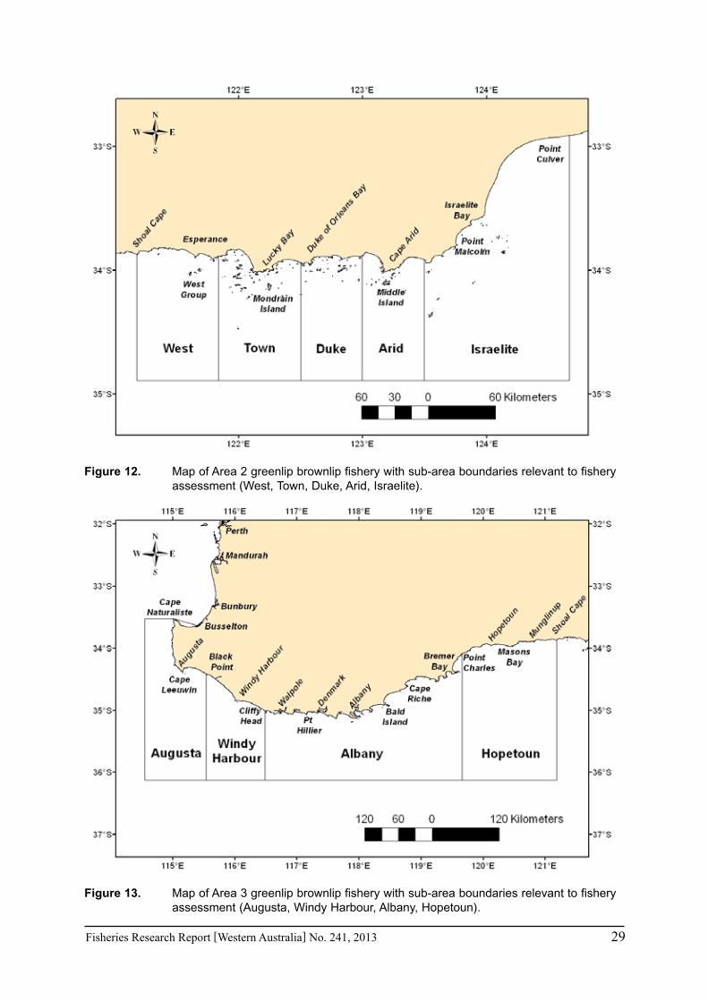
Figure 12. Map of Area 2 greenlip brownlip fishery with sub-area boundaries relevant to fishery assessment (West, Town, Duke, Arid, Israelite).
Figure 13. Map of Area 3 greenlip brownlip fishery with sub-area boundaries relevant to fishery assessment (Augusta, Windy Harbour, Albany, Hopetoun).

30 Fisheries Research Report [Western Australia] No. 241, 2013
4.4.2 Fishing mortality
4.4.2.1 Data
Commercialgreenlipandbrownlipfishersprovidearandomsampleofshellsharvestedfromeachdaysfishingandthesearecategorizedintorelevantsub-areas(Figure12andFigure13).The current sampling protocol is 10 greenlip shells and 5 brownlip shells from each day of fishing,whichisinaccordancewithastudybyAndrewandChen(1997)whoconcludedthatthe optimal sampling procedure was to maximise the number of diver-days from which samples were collected. Commercial divers also undertake digital video surveys on commercially fishedreefs(seesection4.3.2),fromwhicharandomsampleofabalone(~30%ofthetotal)areselected and measured. The legal size animals from the video survey data are used to estimate fishingmortalitywhereapplicable.
Thissamplingprovideslength-frequencydatatoenableestimationoftotalmortalityandfishingmortality. These datasets are used in the development of performance indicators and TACC assessment processes (see section 7), and to assess the changes in targeting practices between years.
SamplingstatisticsforestimatesoffishingmortalityareprovidedinTable12.
Table 12. Length and morphometry sampling statistics for greenlip and brownlip abalone by year
Year AreaTotal # Divers
# Divers Participating
Greenlip samples
Brownlip samples
1995 3 8 7 2597 425
1996 3 8 8 7549 0
1997 3 8 1 1377 0
2004 2 6 5 1525 422
3 8 8 2017 533
2005 2 6 5 1814 481
3 8 4 3004 625
2006 2 6 0 0 0
3 8 3 1102 292
2007 2 6 5 1494 465
3 8 5 1763 436
2008 2 6 3 1086 271
3 8 6 2031 952
2009 2 6 4 821 463
3 8 7 3190 1140
2010 2 6 1 287 261
3 8 8 2783 523
2011 2 6 1 232 103
3 8 5 775 157
4.4.2.2 Estimation methodology
The large variation in growth of abalone (see Figure 7), coupled with the inability to estimate age with any degree of accuracy precludes the use of age-based estimation methodologies forascertainingtotalandfishingmortality.Consequentlyalength-basedcatch-curveanalysismethod is used (Pauly, 1984). The main assumptions of this are that growth, recruitment and

Fisheries Research Report [Western Australia] No. 241, 2013 31
natural mortality parameters are constant from year to year. None of these assumptions are likely to hold strictly true, however they facilitate an estimate of relativefishingmortalitythatiscomparable between years, and relatively robust to violations of the assumptions. For example, an increase in growth rates or recruitment under a constant catch is likely to shift the frequency of the median length-class upward, which would result in a reduction in fishingmortalityestimates. The catch curve equation is of the form;
whereZistotalmortality,Ni is the number of abalone in length class i, dli/dt is the growth rate (mm year –1) of length class i, and ti is the relative age of length class i. Following an estimation of-Zfromtheslopeoftheequation,fishingmortality(F)=Z–M,whereMisassumedtobe0.25 for the harvested size-classes.
Anexample of length frequencydata fromgreenlip abalonefishing in 2010 andparametervalues used in the catch curve analysis are summarised in Table 13. Note that the mode of the size distribution differs between spatial areas (Figure 18), which relates to different growth and selectivity. Full selectivity is not assumed until the modal size class.
Table 13. Length-frequency data (Ni) and catch-curve parameters used in the estimation of total (Z) and fishing (F) mortality in the Western Australian Haliotis laevigata fisheries. Data are from the 2010/11 fishing season.
FisheryLength class
midpoint (mm)Ni dli / dt
Relative age (ti)
Ln[Ni(dli / dt)]
Area 3 South Coast
von Bertalanffy growth parameters: K = 0.25; L∞ = 179 mm
152.5 222 6.9 6.33 7.334
157.5 254 5.5 7.08 7.242
162.5 197 4.3 7.92 6.741
167.5 81 3.0 9.17 5.493
172.5 40 1.7 11.08 4.22
Area 3 WestCoast
von Bertalanffy growth parameters: K = 0.30; L∞ = 185 mm
162.5 365 5.9 7.00 7.675
167.5 303 4.6 7.83 7.240
172.5 218 3.2 9.00 6.548
177.5 109 2.0 10.67 5.385
4.4.3 Yield-per-recruit and egg-per-recruit analyses
Yield-per-recruit (YPR) and egg-per-recruit (EPR) analysis was undertaken for three greenlip abalone populations, Area 2, Area 3 South Coast, and Area 3 West Coast using the PREP model (Shepherd and Baker, 1998). The PREP (Per-Recruit Population Egg Production) model is an age-structured dynamic pool model based on Baranov’s (1918) catch equation. Time steps in the model are monthly time-steps.
In the model the spawning potential of each age class cohort, based on the length-fecundity relationship, is summed from size at reproductive maturity to maximum age (16 years) for an unfishedstock.This is therelativepopulationeggproductionperrecruit (PREP).SpawningpotentialofthefishedstockundervariouslevelsofFisevaluatedandexpressedasapercentageofthespawningpotentialfortheunfishedcohort(%EPR).

32 Fisheries Research Report [Western Australia] No. 241, 2013
Thepercentageyieldperrecruit(%YPR)isobtainedinasimilarmanner.Firstly,themaximumbiomassofthecohortattainableatoptimumsizeatfirstcaptureandoptimalF,fortherelevantgrowth parameters and length-weight relationship, is estimated by iteration. Then the yield-per-recruitundervariouslevelsofFandsizeatfirstcaptureissummedoverallageclasses,andexpressedasa%ofthemaximumpossibleyield(%YPR).Thesize-at-firstcaptureisnottheminimum legal length, but the size at which animals are actually harvested by the commercial fishery,whichishigherthantheLML.
4.4.3.1 Sensitivity analysis
Due to the variability in growth it was necessary to make assumptions of average growth. Growth and fecundity parameters assumed for the YPR and EPR analyses are summarised in Table 3 and Table 4 respectively. Sensitivity analyses to different growth parameters were also undertaken using the Augusta population as a test case, where a tagging study resulted in growth parameters of K = 0.55, and L∞ = 170 mm (Table 3).
4.5 Other Research Projects
4.5.1 Stock enhancement research (Haliotis laevigata)
A series of experiments on stock enhancement of greenlip abalone have been carried out in collaborationwithindustrydiverssince2004.Preliminaryanalysesandresearchfindingsaresummarised in Hart et al. (2007). In 2008 a further experiment was initiated at Flinders Bay, Augusta. This experiment involved the release of abalone at high density at 3 sites, with 11,000 animals of 20 – 30 mm (1+ age) released at an approximate density of 18 – 20 juveniles m-2. The animals were bred from wild broodstock obtained from Augusta in November 2006. Control sites and effects of the enhancement on the habitat and other species are also being examined at part of this research.
In 2009, the Australian Seafood CRC (Cooperative Research Centre) awarded an externally fundedresearchproject.Theprojectwascalled“Bioeconomicevaluationofcommercialscalestockenhancementinabalone”,withtheobjectivestoundertakeacomprehensiveevaluationofthe feasibility for stock enhancement in abalone over 2009 to 2012. Relevant publications from this work can be found in Hart et. al., (in press a; in press b; in press c).
4.5.2 Recovering a collapsed abalone stock through translocation
ThisprojectisinresponsetoacatastrophicmortalityofanabalonefisheryinWesternAustraliadue to an anomalous environmental event in the summer of 2010/11. During this event, termed a“marineheatwave”(Pearceet.al.,2011),seasurfacetemperature(SST)rosetolethallevelsfor this species (roe’s abalone) and, coupled with deoxgenation of the water during an extended calm period, effectively wiped out an entire stock. The project arose following a complete closureofthefisherytoprotectanyremainingstockandadesirebytheindustrytoexaminethepossibility of assisted recovery.
The project has been funded by the Australian Seafood CRC (Cooperative Research Centre), meetstheCRC’sFutureHarvestThemeOutcomes1and2,andisentitled“CRCproject2011/762Recoveringacollapsedabalonestockthroughtranslocation.”Thestudyisamajorcollaborationbetween Industry partners WAFIC, who are providing $81,519 as a cash contribution, the Department of Fisheries WA, Flinders University South Australia, and the Seafood CRC. The

Fisheries Research Report [Western Australia] No. 241, 2013 33
objectives of this project are as follows:
1. To establish founder populations of roe’s abalone in areas of mass mortality
2. To evaluate the genetic structure of existing and founder populations
3. To compare natural and assisted recovery rates of roe’s abalone populations
4. To evaluate the genetic contribution of existing and founder populations to stock recovery
4.5.3 Brownlip abalone: Exploration of wild and cultured harvest potential
Brownlip abalone (Haliotis conicopora) is the largest and possibly fastest growing abalone species in Australia. It is a characteristically unique abalone species, reaching considerably larger maximum sizes (>230 mm), than greenlip (200 mm) and displaying very cryptic behaviour within an extremely limited habitat of caves and crevices. Due to its large size and high meat yield(approx.35%greatermeatweightperlengththangreenlipabalone)itisextremelysuitablefor the lucrative wild and brand new cultured or ocean grown, whole meat export markets.
Brownlip abalone currently comprises a small, but very valuable component of the commercial wildabalonefisheryinWA(annualvalue:$1.6million)andsince1998,annualcatcheshaverisenby25% toover40 tonnes.This increase indemandhas caused anecessity to furtherexplore the brownlip abalone wild, ocean grown and cultured harvest potentials. There is currently however, limited information on habitat, growth and mortality of wild populations and the understanding of aquaculture systems and growth rates. The objectives of the project are as follows:
1. Determine the growth and natural mortality of wild brownlip abalone populations.
2. Determine growth rates and mortality of cultured brownlip abalone.
3. Habitat identification to determine release mortality, growth, survival and recaptureparameters for potential brownlip abalone stock enhancement.
4. Developfishingsizelimitsandoptimalmarketsizesbasedonsizedistributionandgrowthto examine the harvest potential of the total industry
The project has been funded by the Fisheries Research and Development Corporation (FRDC).
4.5.4 Marine Park Abalone surveys: Cape Leeuwin – Cape Naturaliste
In 2007, a series of abalone surveys were undertaken in areas proposed as sanctuary zones in the proposed Capes-Capes marine park as well as control areas. These areas were designed to estimate total abalone biomass in the sanctuary zones, to provide more information on what quantityofcatchmightbeforegoneasaresultoftheclosureofabalonefishinginthesezones.These survey sites will be visited on a periodic basis following the implementation of the Marine Park. Further details are available in Hesp et al., (2008).

34 Fisheries Research Report [Western Australia] No. 241, 2013
5.0 Greenlip and Brownlip Abalone
5.1 Commercial fisheries
5.1.1 Total Catch, effort and CPUE
In 2011 the greenlip/brownlip catch was 202 tonnes whole weight (Table 14), which was similar tothe2010catchof205t.TheArea1(Nullarborfishery)exploratoryquotaremainedat1.2tbutwasnotfishedin2011.
The greenlip catch of 165.9 t whole weight from a total quota of 173.3 t, was very similiar to the2010catchof165.6t.Thebrownlipcatchof36twholeweightforthe2010seasonwas8%lowerthanthe2010catchof39t,andrepresents91%ofthequotaof39.9t(Table14).
Totalfishingeffortonthemainstocksin2011was1,224days.Thiswas2%higherthanin2010(1,196 days).
Catch per unit effort: The commercial divers’ standardised catch rates (SCPUE) are the principal indicator of the abundance of legal-sized abalone and are assessed annually.
In 2011, the SCPUE for the combined greenlip stocks was 35 kg whole weight per hour (Table 14). This was a decrease from the 2010 value of 37 kg per hour.

Fisheries Research Report [Western Australia] No. 241, 2013 35
Table 14. Greenlip and brownlip abalone catch and effort by quota period
Quota period2
Greenlip TAC kg whole weight
Greenlip caught
kg whole weight (all
stocks)
Brownlip TAC kg whole weight
Brownlip caught
kg whole weight4
Combined catch kg
whole weight
Diver days (main stocks only)3
Greenlip standardised
CPUE (kg whole weight) per diver hour
1989 229,619 – 36,977 266,596 1,324
1990 126,500 118,395 – 19,118 137,514 696
1991 148,500 132,194 – 14,658 146,852 816
1992 192,500 170,608 – 30,404 201,012 1,120 37
1993 197,450 173,397 – 31,153 204,550 1,238 37
1994 200,750 171,820 – 32,222 204,042 1,337 36
1995 187,264 145,467 – 27,061 172,528 1,087 32
1996 189,750 171,337 – 21,932 193,269 904 40
1997 207,350 182,317 – 26,297 208,614 1,059 35
1998 200,750 181,810 – 22,197 204,006 1,031 36
1999 184,023 175,765 28,0005 28,047 203,812 922 39
2000 194,691 189,511 34,875 34,179 223,690 1,029 41
2001 194,691 187,459 33,075 31,091 218,550 1,002 37
2002 194,691 166,828 33,075 27,458 194,286 1,027 34
2003 202,521 180,730 37,453 33,449 214,179 1,1443 33
2004 190,520 170,385 35,000 34,196 204,581 1,1543 34
2005 171,755 169,285 38,500 38,745 208,030 1,252 31
2006 171,755 168,752 39,750 37,265 206,017 1,161 31
2007 171,755 166,647 39,750 38,660 205,307 1,139 34
2008 163,220 157,224 41,900 39,515 196,739 1,144 34
2009 171,301 160,156 41,900 39,050 199,206 1,205 34
2010 171,221 165,558 41,900 39,006 204,564 1,196 37
2011 173,355 165,927 39,950 36,274 202,201 1,224 35
1. Data source: quota returns.
2. The length of quota period has varied with management changes, and for simplicity has been recorded against the nearest calendar year.
3. Effort(diverdays):mainstocksareseparatedfromstuntedstocks,whicharesubjecttocontrolledfishingregimesandnotdirectlycomparable.
4. Greenlip conversion factor (meat weight to whole weight) is 2.667. Brownlip conversion factor for meat weight to whole weight is 2.5.
5. BrownlipallocationsnotfixedacrossAreas2and3(ex-Zone1and2)priorto1999.BrownlipTACfixedforthefirstyearin1999.

36 Fisheries Research Report [Western Australia] No. 241, 2013
5.1.2 Catch, CPUE and meat weights by subregion
Thegreenlip-brownlipfisheryconsistsofthreemainmanagementzones(Area1,2,and3;Figure1),however99%ofthecatchcomesfromtheArea2andArea3fisheries.Trendsincatch, CPUE, and average size (meat weight) of greenlip abalone caught in the subregions of theArea2andArea3fisheriesareprovidedbelow.SeeFigure12andFigure13formapsofthe subregions.
5.1.2.1 Area 2 fishery
TheArea2greenlipfisheryisdividedupinto5mainsubregions.Thetwomostimportantregions are Town and Arid (Figure 14), collectively providing an average of 6.1 and 7.6 tonnes respectively of the historical catch. Average catch in the other regions was 3.3 (West), 5.5 (Duke), and 4.0 tonnes (Israelite) (Figure 14). Trends in the catch, catch rate, and meat weight indicatorshavebeenstableover the last20years,althoughsignificantoscillationshave occurred.
AlargersizelimitisfishedintheWestpopulations,asindicatedbythehigheraveragemeatweight of 192 g, compared to the Town (178 g), Duke (181 g), Arid (181 g) and Israelite (187 g). Average catch rate is very similar between areas, varying only 2 kg/hr between the lowest (West – 14 kg/hr) and highest (Arid – 16 kg/hr).
5.1.2.2 Area 3 fishery
TheArea3greenlipfisheryisdividedupinto4mainsubregions.Themostimportantregionis Augusta (Figure 15), providing an annual average of 18 tonnes of the historical catch. Average catch in the other regions was 4 (Windy), 2 (Albany), and 11 tonnes (Hopetoun) (Figure 15). Trends in the catch, catch rate, and meat weight indicators have been stable over thelast20years,althoughsignificantoscillationshaveoccurredintheAugustaandHopetounpopulations.
AlargersizelimitisfishedintheAugustapopulation,asindicatedbythehigheraveragemeatweight of 244 g, compared to the Windy (192 g), Albany (193 g) and Hopetoun populations (195 g; Figure 15). Average catch rate is also highest in Augusta (19 kg/hr), and similar between Windy (14 kg/hr), Albany (15 kg/hr), and Hopetoun (15 kg/hr).
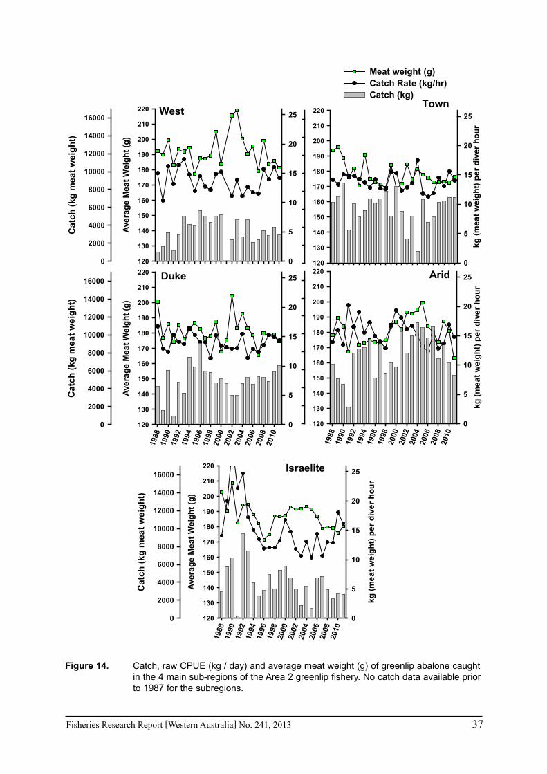
Fisheries Research Report [Western Australia] No. 241, 2013 37
Town
1988
1990
1992
1994
1996
1998
2000
2002
2004
2006
2008
2010
Ave
rag
e M
ea
t W
eig
ht
(g)
120
130
140
150
160
170
180
190
200
210
220
0
5
10
15
20
25
Cat
ch (
kg m
eat
wei
gh
t)
0
2000
4000
6000
8000
10000
12000
14000
16000 Duke
Ave
rag
e M
ea
t W
eig
ht
(g)
120
130
140
150
160
170
180
190
200
210
220
0
5
10
15
20
25
Cat
ch (
kg m
eat
wei
gh
t)
0
2000
4000
6000
8000
10000
12000
14000
16000West
120
130
140
150
160
170
180
190
200
210
220
kg
(m
ea
t w
eig
ht)
pe
r d
ive
r h
ou
r
0
5
10
15
20
25
Meat weight (g)Catch Rate (kg/hr)Catch (kg)
1988
1990
1992
1994
1996
1998
2000
2002
2004
2006
2008
2010
120
130
140
150
160
170
180
190
200
210
220
kg
(m
ea
t w
eig
ht)
pe
r d
ive
r h
ou
r
0
5
10
15
20
25Arid
1988
1990
1992
1994
1996
1998
2000
2002
2004
2006
2008
2010
Ave
rag
e M
ea
t W
eig
ht
(g)
120
130
140
150
160
170
180
190
200
210
220
kg
(m
ea
t w
eig
ht)
pe
r d
ive
r h
ou
r
0
5
10
15
20
25
Cat
ch (
kg m
eat
wei
gh
t)
0
2000
4000
6000
8000
10000
12000
14000
16000Israelite
Figure 14. Catch, raw CPUE (kg / day) and average meat weight (g) of greenlip abalone caught in the 4 main sub-regions of the Area 2 greenlip fishery. No catch data available prior to 1987 for the subregions.

38 Fisheries Research Report [Western Australia] No. 241, 2013
1988
1990
1992
1994
1996
1998
2000
2002
2004
2006
2008
2010
Ave
rag
e M
ea
t W
eig
ht
(g)
120
140
160
180
200
220
240
260
280
0
5
10
15
20
25
30
35
Cat
ch (
kg m
eat
wei
gh
t)
0
5000
10000
15000
20000
25000
30000
35000
40000 Albany
Ave
rag
e M
ea
t W
eig
ht
(g)
120
140
160
180
200
220
240
260
280
0
5
10
15
20
25
30
35
Cat
ch (
kg m
eat
wei
gh
t)
0
5000
10000
15000
20000
25000
30000
35000
40000 Augusta
120
140
160
180
200
220
240
260
280
kg
(m
ea
t w
eig
ht)
pe
r h
ou
r
0
5
10
15
20
25
30
35
1988
1990
1992
1994
1996
1998
2000
2002
2004
2006
2008
2010
120
140
160
180
200
220
240
260
280
kg
(m
ea
t w
eig
ht)
pe
r h
ou
r
0
5
10
15
20
25
30
35Hopetoun
Windy
Meat weight (g)Kg per hourCatch (kg meat weight)
Figure 15. Catch, raw CPUE (kg / day) and average meat weight (g) of greenlip abalone caught in the 4 main sub-regions of the Area 3 greenlip fishery. No catch data available prior to 1987 for the subregions.
5.1.3 Standardised CPUE
StandardisedCPUEinthetwomaingreenlipabalonefisheriesarecurrentlymid-rangeofthelong-termhistoricaltrend,whichappearstoberelativelystable(Figure16).TheArea2fisheryshoweda7%increasefrom2007to2011,whileArea3fisheryhadstablecatchratesinthisperiod (Figure 16).

Fisheries Research Report [Western Australia] No. 241, 2013 39
Figure 16. Standardised meat weight CPUE (kg/hr) of Haliotis laevigata in Area 2 and Area 3.
5.1.4 Average meat weight and length-frequency of catch
Average meat weight of greenlip abalone in Area 2 decreased from 2002 to 2011, and is currently at its lowest historical level (Figure 17). In Area 3, average meat weight dropped from 2007 to 2009 however shell length has been stable between 2004 and 2011 (Figure 17). Overall, alargersize-rangeandaveragesizeiscaught in theArea3,comparedtotheArea2fishery(Figure18).IntheArea3fishery,60%ofthecatchisgreaterthan160mmshelllength,whereasintheArea2fishery,only25%ofthecatchisabove160mm(Figure18).
AveragemeatweightandlengthofbrownlipharvestedintheArea2fisherydecreasedbetween2004 and 2011 and are currently at a low level compared to historical averages (Figure 19). In theArea3fisheryaveragemeatweightandshelllengthofbrownlipabalonehasgenerallybeenstable with the exception of 2011, which saw a large drop in average meat weight from 2010, butthisdeclinewasnotreflectedinmeanlength,whichremainedstable(Figure20).

40 Fisheries Research Report [Western Australia] No. 241, 2013
Area 2
19921994
19961998
20002002
20042006
20082010
Mea
n w
eig
ht
(g)
170
180
190
200
210
220
230
260
mean weight (g)mean length (mm)
Area 3
19921994
19961998
20002002
20042006
20082010
Mea
n le
ng
th (
mm
)
150
152
154
156
158
160
162
164
166
168
170
Figure 17. Mean meat weight (g) and shell length (mm) of Haliotis laevigata harvested from the Area 2 and Area 3 fisheries.
Figure 18. Size-frequency of the catch of Haliotis laevigata from the Area 2 and Area 3 fisheries during 2011. Legal minimum length is 140 mm.

Fisheries Research Report [Western Australia] No. 241, 2013 41
Figure 19. Mean meat weight (g) and shell length (mm) of Haliotis conicopora in the Area 2
and Area 3 fisheries.
Figure 20. Size-frequency of the catch of Haliotis conicopora from the Area 2 fishery and Area 3 fishery in 2010. Sufficient data is not available for 2011. Legal minimum length is 140 mm.

42 Fisheries Research Report [Western Australia] No. 241, 2013
5.1.5 Fishing mortality
FishingmortalitydeclinedsignificantlyintheArea3greenlipfisherybetween2007and2008,particularly on the South Coast (Figure 21a), but then increased again over 2009 to 2011. In the Area2fisheryitdecreasedonlyslightlyoverthesametimeperiod.Inthebrownlipfisheries,fishingmortalitydeclinedinArea2in2004andhassincebeenrelativelyconstantinbothareas(Figure 21b).
Figure 21. Fishing Mortality (F) for greenlip (a) and brownlip (b) abalone. Estimates of F apply only to harvest size animals, and are derived from catch-curve analysis using length-frequency data. See section 4.4.2 for methods.

Fisheries Research Report [Western Australia] No. 241, 2013 43
5.2 Stunted stocks
5.2.1 Stunted individuals
Typical indicators of stunting in individual abalone include the shape of the shell, usually deeper, shorter and/or possibly bowed at the ventral margin (Figure 22e and f). Stunted animals usually have increased growth in depth rather than length, reducing the length-width ratio and producing a more rounded shell (Figure 22b and c). Shells can be thick and unusually heavy or light, thin and weakened by boring organisms. The ventral surface of the shell can have distortions,blistering,uneventextureandspiraclescanbefilledinoraspiraclechannelmayhave formed (Figure 22d). Stunted animals generally have more encrusting animals on the back of the shell, and the ventral surface of the shell may have staining and the nacre can lack lustre (Figure 22d). Quantitative morphometric indicators that depict stunting in commercial shell samples of abalone have been developed (Saunders et al., 2009).
5.2.2 Stunted populations
Abalone that fail to reach their full growth potential have traditionally been considered stunted. However as shown in Figure 7, the full growth potential varies considerably within and between regions and habitats. Stunted populations have been described as: populations whose individuals grow slowly and/or grow to a smaller maximum size in comparison with other populations (Shepherd, 1988; Wells and Mulvay, 1995). Also stunted populations have been hypothesised to have wider, heavier, and deeper shells for a given length, in comparison to their fastergrowingconspecifics(Worthingtonetal.,1995).
ToobtainapracticalworkingdefinitionforstuntedgreenlipstocksinWesternAustralia,stockstructure from in-water stock surveys (see section 4.3.1) was compared with growth parameters frommark-recapture studies at representative populations. Overall, 92% (r2 = 0.92) of the variability in the mean growth parameter (L∞) could be explained by the variability in mean lengthofthepopulationmeasuredfromfisheryindependentsurveys(Figure23).
Based on these results and the equation in Figure 23, we applied a working definition of“stunted”stocksasthosepopulationswherethemaximumtheoreticallengthislessthan140mm. This equates to a mean population length, as measured by in-water stock surveys, of less than 115mm (Figure 23).

44 Fisheries Research Report [Western Australia] No. 241, 2013
Figure 22. Comparison of slow (stunted) and fast growing H. laevigata shells from Hopetoun, Western Australia: a & b. Fast growing shell (longer) and slow growing shell (shorter) with very similar heights (age and maturity). c. Variable heights of slow growing shell, old deep-cupped shells to shallow young shell. d. Thick shells that lack lustre with blistering and discoloured ventral margins is typical of old slow growing animals, however healthy shells with a good lustre are also common. e, f & g. Typical slow growing stunted shells with irregular growth causing distortions in the shape of the shells (greater width and height). h. Ventral view of shells from animals of the same age but with significantly different growth.
a. e.
b. f.
c. g.
d. h.
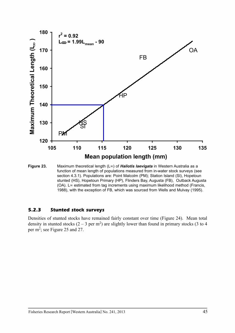
Fisheries Research Report [Western Australia] No. 241, 2013 45
Mean population length (mm)
105 110 115 120 125 130 135
Max
imu
m T
heo
reti
cal L
eng
th (
L
)
120
130
140
150
160
170
180
PM SI HS
HP
FB OA
r2 = 0.92L = 1.99Lmean - 90
Figure 23. Maximum theoretical length (L∞) of Haliotis laevigata in Western Australia as a function of mean length of populations measured from in-water stock surveys (see section 4.3.1). Populations are: Point Malcolm (PM); Station Island (SI), Hopetoun stunted (HS), Hopetoun Primary (HP), Flinders Bay, Augusta (FB), Outback Augusta (OA). L∞ estimated from tag increments using maximum likelihood method (Francis, 1988), with the exception of FB, which was sourced from Wells and Mulvay (1995).
5.2.3 Stunted stock surveys
Densities of stunted stocks have remained fairly constant over time (Figure 24). Mean total density in stunted stocks (2 – 3 per m2) are slightly lower than found in primary stocks (3 to 4 per m2; see Figure 25 and 27.

46 Fisheries Research Report [Western Australia] No. 241, 2013
Years
200
5 2
006
200
7 2
008
200
5 2
006
200
7 2
008
200
5 2
006
200
7 2
008
200
5 2
006
200
7 2
008
200
5 2
006
200
7 2
008
De
ns
ity
pe
r m
2 of
ha
bit
at
0.0
0.5
1.0
1.5
2.0
2.5
3.0Total density< 80 mm (Age 2 - 3)80 - 104 mm (3+)105 - 119 mm (4+)120 - 129 mm (5+)130+ mm (6+)
200
5 2
006
200
7 2
008
De
ns
ity
pe
r m
2 of
ha
bit
at
0
1
2
3
4
5
6
Figure 24. Densities (± 95% CL) of stunted stocks of Haliotis laevigata from research surveys for each size/age class in Western Australian fishery. Data are least-squares mean density and age groupings are approximate only. The right vertical axis is relevant
for the total density and the left axis for the individual length classes.
5.2.4 Managing harvest from stunted stocks
Stuntedstocksarefishedasauniquefishingepisode(calleda“fishdown”). ATACC, legalminimum size (Table 15), and duration of fishing, usually about 2weeks, are set for eachepisode,andtheremainderofthecommercialfisheryisclosedforthatperiod.Thiscontrolstheharvestandsimplifiesthecompliancetaskofpolicinganappropriatesize-limit.
From 1998 to 2011, 78 t of catch was taken from stunted stocks, usually at a legal minimum length of 115 – 120 mm (Table 15). Average weight of individual animals was around 110 – 130 g, compared to 180 – 230g for normal commercial stocks (Figure 17).

Fisheries Research Report [Western Australia] No. 241, 2013 47
Table 15. Location, population data, and fishery statistics of stunted stocks of Haliotis laevigata fished in Western Australia
Location*Mean shell
length (mm)
No. of fishing
episodes
Mean TACC (kg)
LML (mm)Total Catch
(kg)
Average weight
(g)
Augusta 107 3 2,000 130 7,100 140
Hopetoun 109 7 3,700 115 19,800 128
Cape Arid 108 3 5,700 115 14,200 125
Israelite Bay
104 8 4,600 115 – 120 33,800 106
Area 1 5 1,200 110 – 120 4,000 99
TOTAL 78,900
* fromfishery-independentstocksurveys
5.3 Recreational fisheries
5.3.1 Catch, effort and CPUE
The estimated recreational catch of greenlip and brownlip abalone in 2007 was 8 tonnes, whichcomprisedaround3.5%oftotalcatch(Table16).Thisissimilartothe2006estimate.It ispossible that therewere species identification issuesbetweenbrownlipandgreenlipasthe brownlip catch in 2004 and 2006 appears high relative to the greenlip catch. Total effort (11,200days)andaverageCPUE(1.4abaloneperday) for thegreenlipbrownlipfishery in2007 was similar to 2006, which had a total effort of 10,800 days and an average CPUE of 1.4 abaloneperfisherday(Table16).Notelephonediarysurveyswereundertakenin2008–2011.
Table 16. Summary of telephone diary surveys of recreational effort (fisher days), catch rate (abalone per fisher day) and catch (tonnes whole weight) for the greenlip and brownlip abalone fisheries in 2004, 2006, and 2007
Location Year EffortGreenlip Brownlip
Catch RateCatch
(tonnes)Catch Rate
Catch (tonnes)
West Coast
200410,100
(6,500–13,600)0.6 4 (2–6) 0.4 3 (1–5)
20068,000
(4,700–11,300)0.3 2 (0–3) 0.4 3 (0–5)
20076,300
(3,800 – 8,800)0.7 3 (0–6) 0.1 <1 (0–1)
South Coast
20042,700
(1,700–3,700)2.4 2 (1–5) <0.1 <1 (0–1)
20062,800
(1,600–3,900)1.6 2 (0–4) 0.5 1 (0–2)
20074,900
(1,700–8,000)1.8 4 (0–8) 0.2 <1 (0–1)

48 Fisheries Research Report [Western Australia] No. 241, 2013
5.4 Fishery-independent stock surveys
5.4.1 Research Diver Transect Surveys
5.4.1.1 Area 2
Ananalysisofdatafromfishery-independentsurveysofgreenlipstocksinArea2wasavailableforthefirsttimein2011.Meantotaldensityvariedbetweensub-areas,rangingfrom3and8m-2butdidnotvarysignificantlyovertime,withtheexceptionofArid(Figure25),whereitdecreased between 2006 and 2008, but increased again to 2012.
Regarding harvest-sized densities (147+ mm), the only sub-area to experience significantchangeindensitywastheDukeregion,wheredensitydeclinedby50%between2007and2009(Figure 25). No recent survey data is available, however the CPUE analysis for Duke showed an increasing trend between 2004 and 2009 (Figure 14), and a slight decline since then (Figure 14).Significantchangesindensitywerealsoobservedforthe<90mmsizeclassatTown,andthe 91 – 114 mm size class at West, but the density was oscillating, not heading in one direction (Figure 25).
Size-frequencyof stocks shows a significant difference in average size of animals betweenthe different sub-areas (Figure 28). For example, both the Augusta and Albany regions have a significantlyhigheraveragesizeofanimal,withagreaterproportionofanimalsintheexploitedsize-classes (Figure 28), compared to the Hopetoun and Windy Harbour regions. All areas show good recruitment of animals below the minimum legal length.

Fisheries Research Report [Western Australia] No. 241, 2013 49
< 90 mm
0.0
0.5
1.0
1.5
2.0
2.5
3.0 91 - 114 mm
115 - 134 mm
0.0
0.5
1.0
1.5
2.0
2.5
3.0
3.5
4.0135 - 146 mm
147+ mm
WEST TOWN DUKE ARID
200
5 2
007
200
9 2
005
200
7 2
009
200
4 2
006
200
8
200
6 2
008
201
2
0.0
0.5
1.0
1.5
2.0
2.5
3.0
3.5Total density
WEST TOWN DUKE ARID
200
5 2
007
200
9 2
005
200
7 2
009
200
4 2
006
200
8
200
6 2
008
201
2
0
2
4
6
8
10
12
Figure 25. Densities (± 95% CL) of Haliotis laevigata over time and subarea in the Area 2 fishery. Sub-areas are West, Town, Duke and Arid and approximate age classes are 2 – 3 (< 90 mm); 3+ (91 – 114 mm); 4+ (115 – 134 mm); 5+ (134 – 144 mm); 6+ (≥ 147 mm). = significant effect of year (p < 0.05)
Den
siti
es p
er m
2

50 Fisheries Research Report [Western Australia] No. 241, 2013
West (2009)n = 650 (18 sites)average = 125 mm
31-3
541
-4551
-5561
-6571
-7581
-8591
-95
101-
105
111-
115
121-
125
131-
135
141-
145
151-
155
161-
165
171-
175
181-
185>1
90
% f
req
uen
cy o
f G
reen
lip
0
2
4
6
8
10
12
14Town (2009)n = 971 (14 sites)average = 116 mm
31-3
541
-4551
-5561
-6571
-7581
-8591
-95
101-
105
111-
115
121-
125
131-
135
141-
145
151-
155
161-
165
171-
175
181-
185>1
900
2
4
6
8
10
12
14
Duke (2008)n = 276 (8 sites)average = 122 mm
31-3
541
-4551
-5561
-6571
-7581
-8591
-95
101-
105
111-
115
121-
125
131-
135
141-
145
151-
155
161-
165
171-
175
181-
185>1
90
% f
req
uen
cy o
f G
reen
lip
0
2
4
6
8
10
12
14Arid (2012)n = 1718 (25 sites)average = 113 mm
31-3
541
-4551
-5561
-6571
-7581
-8591
-95
101-
105
111-
115
121-
125
131-
135
141-
145
151-
155
161-
165
171-
175
181-
185>1
900
2
4
6
8
10
12
14
Area 2 n = 3615 (65 sites)average = 117 mm
Shell length (mm)
31-3
541
-4551
-5561
-6571
-7581
-8591
-95
101-
105
111-
115
121-
125
131-
135
141-
145
151-
155
161-
165
171-
175
181-
185>1
90
% f
req
uen
cy o
f G
reen
lip
0
2
4
6
8
10
12
14
Figure 26. Size-frequency and average size (mm) of Haliotis laevigata from different sub-areas and the whole Area 2 fishery. Shaded area indicates the exploited size-classes (see Figure 18).

Fisheries Research Report [Western Australia] No. 241, 2013 51
5.4.1.2 Area 3
Ananalysisofdatafromfishery-independentsurveysofgreenlipstockswasavailableforthefirsttimein2011.Meantotaldensityvariedbetweensub-areas,rangingfrom2and6m-2 but didnotvarysignificantlyovertime(Figure27).
Regarding harvest-sized densities (147+ mm), the only sub-area to experience significantchangeindensitywastheAugustaregion,wheredensitydeclinedby50%between2004and2008, but remained constant until 2010 (Figure 27). The SCPUE trends oscillated during this time,showinga10%declinebetween2004and2005,butthena30%increaseto2008,whereithasremainedrelatively(Figure16).Significantincreasesinjuveniledensity(<90mmand91 – 114 mm size classes) were observed at Augusta between 2004 and 2010 (Figure 27), butdensitiesinothersub-areasdidnotaltersignificantly.TheexceptionwasWindyHarbour(Windy),whereasignificantdeclineindensityofjuveniles(<90mm)wasobservedbetween2007 and 2012.
Size-frequencyof stocks shows a significant difference in average size of animals betweenthe different sub-areas (Figure 28). For example, both the Augusta and Albany regions have a significantlyhigheraveragesizeofanimal,withagreaterproportionofanimalsintheexploitedsize-classes (Figure 28), compared to the Hopetoun and Windy Harbour regions. All areas show good recruitment of animals below the minimum legal length.

52 Fisheries Research Report [Western Australia] No. 241, 2013
< 90 mm
0.0
0.5
1.0
1.5
2.0 91 - 114 mm
115 - 134 mm
0.0
0.5
1.0
1.5
2.0
2.5
3.0
135 - 146 mm
147+ mm
Augusta Windy Hopetoun Albany 2004
2006 2008
2010 2007
2009 2012
2006 2007
2008 2009
2007 2008
2009
0.0
0.5
1.0
1.5
2.0
2.5
3.0
Total Density
Augusta Windy Hopetoun Albany 2004
2006 2008
2010 2007
2009 2012
2006 2007
2008 2009
2007 2008
2009
0
2
4
6
8
10
Figure 27. Densities of Haliotis laevigata over time and sub-area in the Area 3 fishery. Sub-areas are Augusta, Windy, Hopetoun and Albany (see Figure 13) and approximate age classes are 2 – 3 (< 90 mm); 3+ (91 – 114 mm); 4+ (115 – 134 mm); 5+ (134 – 146 mm); 6+ (≥ 147 mm). = significant effect of year (p < 0.05)
Den
sity
(p
er m
2 o
f h
abit
at)

Fisheries Research Report [Western Australia] No. 241, 2013 53
Augusta (2010)n = 881 (29 sites)average = 124 mm
31-3
541
-4551
-5561
-6571
-7581
-8591
-95
101-
105
111-
115
121-
125
131-
135
141-
145
151-
155
161-
165
171-
175
181-
185>1
90
% f
req
ue
nc
y o
f G
ree
nlip
0
2
4
6
8
10
12Windy Harbour (2009)n = 551 (12 sites)average = 125 mm
31-3
541
-4551
-5561
-6571
-7581
-8591
-95
101-
105
111-
115
121-
125
131-
135
141-
145
151-
155
161-
165
171-
175
181-
185>1
900
2
4
6
8
10
12
Albany (2008)n = 1493 (23 sites)average = 128 mm
31-3
541
-4551
-5561
-6571
-7581
-8591
-95
101-
105
111-
115
121-
125
131-
135
141-
145
151-
155
161-
165
171-
175
181-
185>1
90
% f
req
ue
nc
y o
f G
ree
nlip
0
2
4
6
8
10
12Hopetoun (2009)n = 599 (31 sites)average = 113 mm
31-3
541
-4551
-5561
-6571
-7581
-8591
-95
101-
105
111-
115
121-
125
131-
135
141-
145
151-
155
161-
165
171-
175
181-
185>1
900
2
4
6
8
10
12
Area 3n = 3524 (95 sites)average = 124 mm
Shell length (mm)
31-3
541
-4551
-5561
-6571
-7581
-8591
-95
101-
105
111-
115
121-
125
131-
135
141-
145
151-
155
161-
165
171-
175
181-
185>1
90
% f
req
ue
nc
y o
f G
ree
nlip
0
2
4
6
8
10
12
Figure 28. Size-frequency of Haliotis laevigata from different sub-areas and the whole Area 3 fishery. Shaded area indicates the exploited size-classes (see Figure 18).

54 Fisheries Research Report [Western Australia] No. 241, 2013
5.4.2 Digital video surveys
Digital video surveys of greenlip abalone in Area 2 showed no change in mean abundance over time, with the exception of the 115 – 134 mm size class, which increased at Arid between 2010 and 2011, and the harvestable size class (147 mm+) in the Town sub-region, which declined between 2008 and 2012 (Figure 29).
Size-frequencydatafromtheDVIsurveysshowarelativelystablesize-structurewithconsistentrecruitment(Figure30).Approximately20–25%ofthepopulationisvulnerabletoexploitation,and there is substantial information on pre-recruit size and age classes (Figure 30).
Overall, theDVI surveys are still in the experimental stage, however in theArea 2fisheryappear to be providing a useful survey of abundance and size structure.

Fisheries Research Report [Western Australia] No. 241, 2013 55
< 115 mm
0.0
0.5
1.0
1.5
2.0
2.5
3.0
3.5
115 - 134 mm
Rel
ativ
e ab
un
dan
ce (
abal
on
e p
er m
inu
te)
0
1
2
3
4
5
6
7
8
9135 - 146 mm
147+ mm
WST TOWN DUKE ARID ISR
201
1 2
008
200
9 2
010
201
1 2
012
200
9 2
010
201
2 2
010
201
1 2
010
0.0
0.5
1.0
1.5
2.0
2.5
3.0
3.5
4.0Total
WST TOWN DUKE ARID ISR
201
1 2
008
200
9 2
010
201
1 2
012
200
9 2
010
201
2 2
010
201
1 2
010
0
2
4
6
8
10
12
14
16
18
20
Figure 29. Mean abundance (± 95% CL) of different size classes (mm) of Haliotis laevigata in sub-areas of Area 2 as surveyed by digital video between 2008 and 2011. Sub-area codes are: WST – West, ISR – Israelite. For map of locations see Figure 12. = significant effect of year (p < 0.05)

56 Fisheries Research Report [Western Australia] No. 241, 2013
2008n = 741 (40 sites)average = 132 mm
% f
req
uen
cy o
f G
reen
lip
0
2
4
6
8
10
12
14
2007n = 343 (6 sites)average = 126 mm
% f
req
uen
cy o
f G
reen
lip
0
2
4
6
8
10
12
14
2009n = 1096 (52 sites)average = 131 mm
Shell length (mm)
31-3
541
-4551
-5561
-6571
-7581
-8591
-95
101-
105
111-
115
121-
125
131-
135
141-
145
151-
155
161-
165
171-
175
181-
185>1
90
% f
req
uen
cy o
f G
reen
lip
0
2
4
6
8
10
12
14
2010n = 1457 (73 sites)average = 131 mm
% f
req
uen
cy o
f G
reen
lip
0
2
4
6
8
10
12
14
2011n = 1394 (71 sites)average = 129 mm
% f
req
uen
cy o
f G
reen
lip
0
2
4
6
8
10
12
14
2012n = 484 (26 sites)average = 132 mm
Shell length (mm)
31-3
541
-4551
-5561
-6571
-7581
-8591
-95
101-
105
111-
115
121-
125
131-
135
141-
145
151-
155
161-
165
171-
175
181-
185>1
90
% f
req
uen
cy o
f G
reen
lip
0
2
4
6
8
10
12
14
Figure 30. Size-structure of Haliotis laevigata in the Area 2 fishery, as captured by digital video surveys. Shaded areas indicate abalone of harvestable size (≥ 145 mm).
5.4.3 Discussion: FIS trends and limitations
These results represent the first analyses of fishery-independent survey methodology forHaliotis laevigata stocks in Western Australia. Looking at the transect surveys, total densities varied significantlybetween sub-areas, ranging fromaround6 to8perm2 of habitat in the Arid region of theArea 2fishery (Figure 25) to around2 perm2 in the Augusta region of theArea3fishery (Figure27).This is indicativeofdifferent levelsoffishing intensity and

Fisheries Research Report [Western Australia] No. 241, 2013 57
productivitythroughoutthefishery.Size-frequencydatasupportsthisvariability,forexampleintheAugustaregion,31%ofthestockis≥147 mm (Figure 28), compared to the Arid region whereonly10%ofthestocksare≥147 mm (Figure 26). Coupled with the known variability in growth, these data suggest that regionally focused harvest and management controls are likely tobetheoptimalwayformaintainingasustainablefishery.
Densities over time appear relatively consistent, however significant declines in density ofharvestable animals (147+ mm) was detected in two sub-areas, Town in Area 2, and Augusta in Area 3 between 2006 and 2010. In particular, the decline in densities of 147+ mm animals within theTownsubregionwasdetectedbytwomethods;thefixed-sitetransectsurveys(Figure25),and the random site digital video surveys (Figure 29). Although occurring at slightly different temporal scales (2007 to 2009 for the transect surveys and 2008 – 2011 for the video surveys) due to different sampling regimes, it highlights a potential issue because this sub-area supplies 25%oftheArea2catch.SignificantdeclinesintheCPUEinthesesub-areaswerenotobservedoverthistimeperiod,andfishingmortalityoscillatedwithnoobviousupwardordownwardtrend. Fixed site transect surveys have not been conducted in these areas since 2009 (Town) and 2010 (Augusta), however are planned in 2013.
With only a few temporal data points, the conclusions for most areas are preliminary at this time, and extra surveys are being planned to strengthen the analysis. Once a reasonable time series of data has been established, the surveys will be used to set additional performance indicatorsforthefisherytocomplementthestandardisedCPUEofthefishers.
Overall,theresearchandDVIsurveysprovideanindicationofpre-recruitabundance,whichisnot contained in the SCPUE trends. This will be valuable information for an early detection of anysignificantchangesinrecruitmentpatternsthatmayoccurwithclimatevariations.
5.5 Yield-per-recruit and egg-per-recruit analyses
5.5.1 Modelling under assumed growth parameters
Underthecurrentminimumsizefishedof142mm,greenlipabalonepopulationsintheArea2fisheryhavereachedthemaximumyield-per-recruitpossibleunderthecriteriaofmaintainingstocks above the 50%virgin egg conservation threshold (Figure 31). If theminimum sizefishedisdroppedto135mm,aslightlyhigheryieldperrecruitispossibleundercurrentfishingmortality rates, however egg conservation would fall under the threshold (Figure 31), and the longertermsustainabilityofthefisherymaybeatrisk.
This situation contrasts with theArea 3 fishery. For example, in the South Coast stocks(Albany,Hopetoun,WindyHarbour),theminimumsizefishedof145mmisresultinginegg-conservationlevelsabovethethresholdof50%(Figure32).Themodelshowedthatamodestincreaseinyieldcouldbesustainedbyafishingatasmallerminimumsizefishedof140mm,andthatthiswouldstillresultineggconservationlevelsofaround50%ofvirgin.SimilarlyfortheAugustastocks,currentlevelsoffishingmortalityareproducingaround70%ofmaximumyield-per-recruit at the current minimum size of 153 mm (Figure 33). Yield could be increased by10%simplybymovingtoasmallerminimumsizedfishedof143mm,andeggconservationlevelsof40%ofvirginwouldstillbeattained(Figure33).Todetermineanoptimumleveloffishingitisalsoimportanttoassesstherelativevalueofdifferentsizeabaloneandundertakeavalue-per-recruit analysis.

58 Fisheries Research Report [Western Australia] No. 241, 2013
5.5.2 Sensitivity analysis: varying growth parameters
The sensitivity analyses for the Augusta population, using a different growth curve, produced a similarresulttothemainanalysis.Namelythatcurrentlevelsoffishingmortalityareproducingaround70%ofmaximumyield-per-recruit at the currentminimumsizedfishedof153mm(Figure 34), and that the egg conservation threshold is well exceeded. Yield could be increased by5to10%bymovingtoasmallerminimumsizedfishedof143mm,whilststillmaintainingeggconservationlevelsof40%(Figure34).
The main assumptions of YPR and EPR models of constant growth, mortality and recruitment are not likely to hold true from year to year, and consequently there needs to be a cautious interpretations of their estimates. Nevertheless, the sensitivity analysis did not contradict the overallconclusion,namelythatasmallloweringofsize-limitsmaybebeneficialtotheArea3fisherywithoutcompromisingeggconservationtargets.However,evenifthesetargetswerenotmet under smaller minimum sizes, the implementation of TACC decision rules that use estimates offishingmortalitywillensurethatappropriatereductionsincatchquotascanbeimplementedinresponse to the exceeding of egg conservation targets (see section 7.3 for further details).
Figure 31. % YPR and % EPR versus fishing mortality fate for the Area 2 Haliotis laevigata populations, for the current minimum length of fishing (142 mm), as well as a 135 mm minimum length. Red line is the egg conservation threshold for these stocks (see section 7.3.1), and blue line is the current average fishing mortality over the period 2004 – 2008 (see Figure 21)

Fisheries Research Report [Western Australia] No. 241, 2013 59
Figure 32. % YPR and % EPR versus fishing mortality for the South coast stocks (Albany, Hopetoun, Windy Harbour) of the Area 3 Haliotis laevigata fishery, under the current minimum length of fishing (145 mm), as well as a 140 mm minimum length. Red line is the egg conservation threshold for these stocks (see section 7.3.1), and blue line is the current average fishing mortality over the period 2004 – 2008 (see Figure 21).
Figure 33. % YPR and % EPR versus fishing mortality fate for the West coast stocks (Augusta) of the Area 3 Haliotis laevigata populations, for the current minimum length of fishing (153 mm), as well as a 143 mm minimum length. Red line is the egg conservation threshold for these stocks (see section 7.3.1), and blue line is the current average fishing mortality over the period 2004 – 2008 (see Figure 21). Assumed growth parameters are K =0.3; L∞ = 185 mm.

60 Fisheries Research Report [Western Australia] No. 241, 2013
Figure 34. Sensitivity analysis: % YPR and % EPR versus fishing mortality rate for the West coast stocks (Augusta) of the Area 3 Haliotis laevigata populations, for the current minimum length of fishing (153 mm), as well as a 143 mm minimum length. Red line is the egg conservation threshold for these stocks (see section 7.3.1), and blue line is the current average fishing mortality over the period 2004 – 2008 using the adjusted growth parameters (K = 0.55, L∞ =170). In comparison, growth assumptions for model outputs in Figure 33 are K = 0.30, L∞ =185.

Fisheries Research Report [Western Australia] No. 241, 2013 61
6.0 Roe’s Abalone
6.1 Commercial fisheries
6.1.1 Catch, effort and CPUE
The TACC for the 2011 quota year was 92.8 t whole weight for Roe’s abalone. The 2011 catch of81.6twholeweight(Roe’sAbaloneTable1)was10tonneslowerthan2010andabout90%of the TACC (Table 17). It was also the lowest catch in over 20 years. The overall TACC was notcaughtbecauseArea1wasnotfishedin2011andcatchesinArea5werebelowtheTACC(75%ofTACCcaught)duetounfavourableweather.
TotalTACCisnotusuallycaughtintheRoe’sabalonefisherybecauseofweather-relatedissuesandthefactthatTACCinthemarginalregionsofthefishery(Area1)ismostlyanexploratoryquota.
Area8ofthefisheryalsoexperiencedcatastrophicmortalityofabaloneduetoananomalousenvironmental“marineheatwave”eventinthesummerof2010/11(Pearceetal.2011).Theareawasclosedtofishingpriortothecommencementofthe2011commercialseason.
TotaleffortfordedicatedRoe’sabalonediversin2011was426diverdays,25%lowerthanlastyear’s effort of 567 diver days (Table 17). The effort in 2011, which was the lowest in over 20 years,resultedfromacombinationoflowerquotabeingset,andclosuretotheArea8fishery(that traditionally required between 100 and 150 days).
6.1.2 Standardised CPUE
Standardised CPUE represents the best available long-term abundance index. The SCPUE for dedicated Roe’s abalone divers in 2011 was 30.7 kg/hr, which was slightly higher than the 2010 catch rate (Table 17), and the third highest in over 20 years.
TheArea7fisheryhassustainedthehighestSCPUE,andthishasbeenrelativelystablesince1992.SCPUEinallotherfisherieshasoscillatedupanddownwithnoparticularlong-termtrend. Theexceptions include theArea2fisherywhereSCPUEhadexperiencedanoveralldeclining trend, which has reversed in recent years (Figure 35) and the Area 8 commercial fishery(NorthernRegionforrecreational),whichhasbeenclosedtoallfishingtopromotestockrecovery following mass mortality.

62 Fisheries Research Report [Western Australia] No. 241, 2013
Table 17. Roe’s abalone catch and effort1 by quota period with raw and standardised catch per unit effort (SCPUE).
Quota period2
Roe’s TACCkg whole weight3
Roe’s caughtkg whole
weight
Diver days4
(Roe’s divers only)
Raw CPUE (roei divers) kg per day )
SCPUE (kg per hour)
1990 105,000 116,447 936 112
1991 101,000 109,489 832 118
1992 105,000 111,341 735 134 27.3
1993 128,000 115,281 832 123 29.4
1994 125,960 117,835 908 113 27.7
1995 125,960 114,501 1,047 98 25.5
1996 125,960 118,715 1,004 106 28.8
1997 126,790 118,738 855 120 30.2
1998 93,9605 86,425 695 108 27.9
19996 119,900 112,949 659 149 29.5
2000 115,900 107,735 647 144 28.7
2001 107,900 99,174 685 126 30.0
2002 107,900 100,471 700 125 28.6
2003 110,900 96,005 723 118 29.0
2004 110,900 107,593 736 126 28.0
2005 112,700 96,496 672 131 31.3
2006 112,700 98,370 625 136 33.2
2007 109,700 90,750 585 132 28.5
2008 106,700 93,197 580 133 28.6
2009 101,800 92,838 554 140 29.0
2010 101,800 91,418 567 134 29.5
2011 92,800 81,607 426 157 30.7
Notes
1. Data source: quota returns.
2. The length of quota period has varied with management changes and, for simplicity, has been recorded against the nearest calendar year.
3. Standard conversion factors for meat weight to whole weight for Roe’s abalone were 2.5 prior to 2000 and 3.0 from 2000.
4. Effort (diver days) for dedicated Roe’s divers only.
5. Reduced quota for a 6-month season.
6.In1999,fishingrestrictions(100kgdailycatchlimit)inthePerthmetropolitanareawerelifted.Thishadtheimmediateeffectofdoubling the catch rate (kg/day) in that area.

Fisheries Research Report [Western Australia] No. 241, 2013 63
Area 2S
tan
dar
dis
ed C
PU
E (
kg/h
r)
15
20
25
30
35
40
45
50 Area 5
Area 6
Sta
nd
ard
ised
CP
UE
(kg
/hr)
15
20
25
30
35
40
45
50
Area 7
1992 1993
1994 1995
1996 1997
1998 1999
2000 2001
2002 2003
2004 2005
2006 2007
2008 2009
2010 2011
Area 8
1992 1993
1994 1995
1996 1997
1998 1999
2000 2001
2002 2003
2004 2005
2006 2007
2008 2009
2010 2011
Sta
nd
ard
ised
CP
UE
(kg
/hr)
15
20
25
30
35
40
45
50
Figure 35. Standardised CPUE of Haliotis roei from the six fishery management areas from 1992 to 2009.

64 Fisheries Research Report [Western Australia] No. 241, 2013
6.2 Recreational fisheries
6.2.1 Catch, effort and CPUE
Estimated catch of Roe’s abalone from the Perth metropolitan area in 2011 was 22 t, as estimated fromthefieldsurvey(Table18).Thisisa96%decreaseofthecatchachievedin2010,causedby a combination of decreases in effort and catch rates as a result of poor weather conditions and meat weights (Table 18).
Catch estimates of Roe’s abalone from the phone diary surveys in 2007 were 24.0 t in the Perth metrofishery,9.0tintheWestCoastFishery,and5.3tintheSouthCoastFishery(Table19).These estimates are similar to the 2006 telephone diary survey estimates. The phone diary estimatesforthePerthmetroarewellbelowthefieldestimatesin2006and2007.
Recreationalfishing represented about 22–36%of the total (commercial and recreational)Roe’sabalonecatchacrossthestatein2007.Thisissimilartothe2006estimateof21–34%ofthetotalcatch.AssumingcatchfromtheSouthCoastfisheryremainedsimilarin2011,itwasestimatedthatrecreationalfishingproduced31%ofthetotalRoe’sabalonecatchin2011.
EffortinthePerthfisheryin2011was11,396hours,whichwasa37%decreaseon2010effortof 18,010 hours (Table 18).Effort in 2011was also 24% lower than the 10-year historicalaverageof14,951hours.Thiswasprimarilyduetothepoorweatherconditionsaffectingfisherparticipation. Weather conditions were rated as being the second worst in well over a decade offishing(Figure36).
Effortestimatesforstate-widerecreationalabalonefishingfromthe2007telephonediarysurveywere 13,400 days in the Perth metropolitan area, 6,300 days on the west coast (excluding the Perth metropolitan area), and 4,900 days on the south coast (Table 19). Total effort has slightly declined from 30,000 days in 2004 to 24,600 days in 2007 (Table 19).
6.2.2 Weather conditions and recreational catch
RecreationalcatchinthePerthmetropolitanregionbetween1999and2011wassignificantlyinfluencedbybotheffort(Ei; p = 0.002) and weather conditions (Wi; p = 0.01) in that year (i). Thegoodness-of-fit(R2) to the predictive relationship was 0.79, and the relationship itself was as follows:
logCatchi = –0.183Wi + 0.731 log Ei – 2.946 + εi; R2 = 0.79
Figure 36 shows that catch decreases linearly with an increase in the weather condition index, buttheeffortisalsoequallyimportantinthefinalcatchestimate.

Fisheries Research Report [Western Australia] No. 241, 2013 65
Table 18. Summary of effort (fisher hours), catch rate (abalone per hour), catch (number of abalone and tonnes whole weight) and mean whole weight (g) for the Perth recreational Roe’s abalone fishery, from annual field surveys
Year
Field Survey
Effort(hours)
Catchrate
Catch(number)
Catch(tonnes)
Meanweight (g)
1999 16,449 23 383,600 35.3 92
2000 15,818 21 330,300 30.2 91
2001 17,727 27 481,300 44.1 92
2002 18,127 22 401,500 36.0 90
2003 17,963 26 442,400 42.6 96
2004 14,614 24 342,900 31.7 93
2005 12,328 21 262,700 24.3 92
2006 10,435 29 297,000 30.2 101
2007 12,433 28 338,000 34.4 102
2008 14,490 29 420,000 44.4 106
2009 19,718 27 517,000 48.6 94
2010 18,010 26 468,000 43.9 94
2011 11,396 23 266,202 22.4 84
Table 19. Summary of telephone diary surveys of effort (fisher days), catch rate (abalone per fisher day) and catch (tonnes whole weight) for the Roe’s abalone recreational fisheries in 2004, 2006, and 2007.
Location Year Effort (± Range)Roe’s
Catch Rate Catch (t)
Perth Metro1
2004 17,200 (14,000 – 20,500) 17.8 28 (25 – 31)
2006 12,600 (9,900 – 15,500) 18.2 23 (20 – 26)
2007 13,400 (10,500 – 16,200) 17.6 24 (19 – 29)
West Coast1 (excl. Metro)
2004 10,100 (6,500 – 13,600) 11.0 10 (7 – 14)
2006 8,000 (4,700 – 11,300) 14.7 12 (7 – 17)
2007 6,300 (3,800 – 8,800) 14.1 9 (6 – 12)
South Coast22004 2,700 (1,700 – 3,700) 6.2 2 (1 – 3)
2006 2,800 (1,600 – 3,900) 6.3 2 (1 – 2)
2007 4,900 (1,700 – 8,000) 10.8 5 (1 – 9)
1. Both areas are within the West Coast bioregion.
2. Survey area is South Coast bioregion (i.e. east of Black Point).

66 Fisheries Research Report [Western Australia] No. 241, 2013
Figure 36. Catch of Haliotis roei in the Perth recreational fishery as a function of weather conditions (low index=good conditions for fishing) and varying effort. To show the effect of effort, two effort trajectories (12,000 and 18,000 hours) have been plotted. Table 18 provides the actual effort for each year of harvest. Symbols indicate years, e.g. 01 = 2001. For details of the weather condition index, see Hancock and Caputi (2006).
6.3 Fishery-independent stock surveys
6.3.1 Research Diver Surveys
Densities of individual age classes of Haliotis roei in the Perth metropolitan fishery havesignificantlychangedovertime(Table20;Figure37).The51–60mmsizeclass(Age3+),showsasignificantincreasingtrendbetween2006and2012,butthe≥ 71mm class shows the opposite trend (Figure 37). In early 2012 the proportion of animals ≥ 71mm was very low (Figure38),around5%.
The approximate age classes for Haliotis roei have been determined using a growth curve developed by Hancock (2004). To determine the accuracy of these age classes, correlations were carried out between densities of successive age classes from 0+/1+ to 4+/Recruits with a 1-yearlag.Statisticallysignificantcorrelationsbetween2+/3+(r = 0.93) and 3+/4+ (r = 0.75) were detected, but not for other successive age classes. This may be due to a combination of selectivity, particularly for 0+ age class, the recruit class consisting of multiple year classes, and/or inaccurate assigning of size to age, however the significant correlations suggested apredictive ability in the density surveys, and further work was carried (see section 6.3.2).

Fisheries Research Report [Western Australia] No. 241, 2013 67
Table 20. GLM results for the effect of Year, Habitat, and Location on densities of different size and age classes of Haliotis roei in the Area 7 fishery in Western Australia. Data has been ln (x+1) transformed.
Source of variability
d.f. MS F P MS F P
0+ (< 17 mm) 1+ (17 – 32 mm)
Year 15 11.9 7.42 <0.001 2.59 1.98 0.01
Location 10 12.2 7.59 <0.001 29.5 22.6 <0.001
Habitat 1 207.2 128.7 <0.001 103.6 79.3 <0.001
Residual 823 1.61 1.31
2+ (33 – 50 mm) 3+ (51 – 60 mm)
Year 15 2.53 2.44 0.002 4.29 4.11 <0.001
Location 10 43.3 41.8 <0.001 77.9 74.9 <0.001
Habitat 2 257.3 247.9 <0.001 411.1 394.7 <0.001
Residual 1191 1.04 1.04
4+ (61 – 70 mm) Recruits (³ 71 mm)
Year 15 3.48 2.69 <0.001 8.67 6.8 <0.001
Location 10 85.5 66.2 <0.001 67.8 52.8 <0.001
Habitat 3 352.7 273.1 <0.001 89.1 69.4 <0.001
Residual 2201 1.29

68 Fisheries Research Report [Western Australia] No. 241, 2013
Figure 37. Density trends in Age 0+ (1 – 16 mm ), Age 1+ (17 – 32 mm), 2+ (33 – 50 mm), 3+ (51 – 60 mm), 4+ (61 – 70 mm), and recruited (71+ mm) Haliotis roei in the Area 7 fishery.

Fisheries Research Report [Western Australia] No. 241, 2013 69
Figure 38. Size-frequency (mm) of Haliotis roei in the Peth fishery from 2006 to 2012. Shaded areas indicated size targeted by the fishery. Dotted line is the legal minimum length (60 mm).
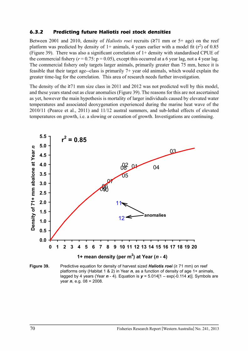
70 Fisheries Research Report [Western Australia] No. 241, 2013
6.3.2 Predicting future Haliotis roei stock densities
Between 2001 and 2010, density of Haliotis roei recruits (≥71 mm or 5+ age) on the reef platformwaspredictedbydensityof1+animals,4yearsearlierwithamodelfit(r2) of 0.85 (Figure39).Therewasalsoasignificantcorrelationof1+densitywithstandardisedCPUEofthecommercialfishery(r = 0.75: p = 0.05), except this occurred at a 6 year lag, not a 4 year lag. Thecommercialfisheryonlytargetslargeranimals,primarilygreaterthan75mm,henceitisfeasible that their target age--class is primarily 7+ year old animals, which would explain the greater time-lag for the correlation. This area of research needs further investigation.
The density of the ≥71 mm size class in 2011 and 2012 was not predicted well by this model, and these years stand out as clear anomalies (Figure 39). The reasons for this are not ascertained as yet, however the main hypothesis is mortality of larger individuals caused by elevated water temperatures and associated deoxygenation experienced during the marine heat wave of the 2010/11 (Pearce et al., 2011) and 11/12 austral summers, and sub-lethal effects of elevated temperatures on growth, i.e. a slowing or cessation of growth. Investigations are continuing.
1+ mean density (per m2) at Year (n - 4)
0 1 2 3 4 5 6 7 8 9 10 11 12 13 14 15 16 17 18 19 20
Den
sity
of
71+
mm
ab
alo
ne
at Y
ear
n
0.0
0.5
1.0
1.5
2.0
2.5
3.0
3.5
4.0
4.5
5.0
5.5
01 02
03
04
05
06 07
08
09 10
11
12
r2 = 0.85
anomalies
Figure 39. Predictive equation for density of harvest sized Haliotis roei (≥ 71 mm) on reef platforms only (Habitat 1 & 2) in Year n, as a function of density of age 1+ animals, lagged by 4 years (Year n - 4). Equation is y = 5.014[1 – exp(-0.114 x)]. Symbols are year n, e.g. 08 = 2008.

Fisheries Research Report [Western Australia] No. 241, 2013 71
7.0 Performance Indicators and TACC Assessment
7.1 Methodology
Development of performance indicators and TACC decision rules in the Western Australian abalonefisheryisanongoingprocess.Progresstodateincludesindicatorsbasedoncommercialfisherycatchrates(Hartetal.,2009),andresearchintoharvestrates(section7.3.1).Thegeneralprotocol is to vary the allowable catch up or down around a sustainable long-term TACC (defined inTable21),basedon therelationshipbetween theperformance indicatorsand thebiological reference points (Figure 40). The adjustment of TACC (both quantity and direction) ismadeaccordingtopre-defineddecisionrules(Table22).ColourcodesdenotingthedecisionrulesforTACCadjustmentinWesternAustralia’scommercialabalonefisheriesaresummarisedin Table 23.
Figure 40. Example of performance indicator using a 3-year moving average (pink line) and biological reference points (Target, Limit, Threshold) for a hypothetical abalone fishery, and a schematic of how TACC would vary over time. Yearly data are standardised CPUE (± 95% CLs), and relative differences (to the threshold BRP) are on the right axis.

72 Fisheries Research Report [Western Australia] No. 241, 2013
Table 21. Biological Reference Points (BRPs) and sustainable TACCs for management areas and species in the Western Australian abalone fisheries. The values of BRP relative to the Threshold level set at 1 are shown in brackets)
Area SpeciesThreshold Reference
Year
Sustainable TACC (t)
2011
Biological Reference Points
Threshold Value* (kg/
hr)
Limit value (20% below Threshold)
Target value (20% above Threshold
2 H. laevigata 2005 30.0# 11.87 (1.0) 9.49 (0.8) 14.24 (1.2)
3 H. laevigata 2004 35.0 12.18 (1.0) 9.74 (0.8) 14.62 (1.2)
2 H. roei 1995 19.8@ 25.07 (1.0) 20.05 (0.8) 30.08 (1.2)
5 H. roei 1993 20.0 22.19 (1.0) 17.75 (0.8) 26.62 (1.2)
6 H. roei 1993 12.0 21.93 (1.0) 17.54 (0.8) 26.31 (1.2)
7 H. roei 1998 36.0 35.80 (1.0) 28.64 (0.8) 42.96 (1.2)
8 H. roei 1998 0.0** - - -# H. laevigata TACC in meat weight;@ H. roei TACC in whole weight* Current threshold value (as of February 2012), however will vary with future updates of the SCPUE model,
and new values will be reported each year.** Area8closedindefinitelyduetoenvironmentallyinducedmassmortality(Pearceet.al.,2011)
Table 22. Management decision rules in relation to defined biological reference points (BRPs) for Western Australian Abalone Fisheries. See Figure 40 for the relationship between the performance indicator and biological reference points.
BRPs Description Decision Rule
Target 20% above Threshold Minimum of 10% TACC increase if PI is above the target BRP
Threshold upper end of the bottom 30% of the historical variability in the PI
a) Maintain TACC at long-term sustainable level if PI is above threshold and below target BRP
b) 10% TACC decrease (below long-term sustainable level) if PI is below threshold and above limit BRP
Limit 20% below Threshold Minimum of 30% TACC decrease if PI is below limit BRP
Table 23. TACC decision rules for Western Australian Abalone Fisheries. These operate in relation to defined performance indicators (see Table 24).
Colour Code TACC Decision
Minimum of 30% TACC decrease
10% TACC decrease below long-term sustainable levels
Maintain TACC at long-term sustainable levels
Minimum of 10% TACC increase above long-term sustainable levels
7.2 2012/13 TACC Assessments
The 2012/13 TACC decisions using the current decision rule framework are summarised in Table24.Theperformanceindicator(PI)wasabovethethresholdvalueinallfisheriesthatwereassessed.UsingtheArea2greenlipfisheryasanexampleoftheprocess,Table24showsthatthe performance indicator (PI) had a value of 13.6, which was above the threshold value (11.87). Consequently the decision rule concluded a blue result, i.e. that TACC should be set at the long-term sustainable level (30.0 t). After industry consultation on stock status, and examination of the outcome of new harvest control rule that incorporate egg conservation targets achieved

Fisheries Research Report [Western Australia] No. 241, 2013 73
thoughfishingmortalityindicators(section7.3.2),aprecautionaryapproachwasadoptedforArea2andTACCmaintainedat28.8 t.AgraphicalsummaryofPI trends inallfisheries isprovided in section 11.1.
The basis for setting of brownlip abalone quota is less formalised than greenlip abalone, and is currently under review as part of an external project (see section 4.5.3). The procedure at present is based on an examination of historical trends in catch and meat weight, and feedback from industry. Quota reductions were taken in the 2011/12 season due to concerns over declining meat weights (see Figure 19).
The decision rule framework provides a level of certainty to the TACC process; in particular what changes could be expected under different scenarios. However the final decision onquotas is not entirely based on its outcomes, as the data used in the decision rule is not without uncertainty. Stakeholder input into the assessment process is an integral part of the decision-making process.
7.2.1 Fishery closures
TheArea8roe’sabalonecommercialfishery(seeFigure2),andthenorthernsectionof therecreationalabalonefishery(seeFigure3)havebeenclosedunderasection43orderandnoTACC is recommended for 2012/13. In the summer of 2010/11, the abalone stocks in Kalbarri region suffered a devastating mortality as result of a sustained period of elevated water temperatures,nowbeingtermedthe“2011marineheatwave”offWesternAustralia(Pearceet.al.,2011).Bothcommercialandrecreationalabalonefisherieshavebeenclosedtoprotectanyremaininganimalsandpromotenaturalrecovery.Thesevereextentofthemortality(>99.9%inmost places) means that natural recovery is unlikely within the next 10 years. A research project has been funded to evaluate the possibility of assisted recovery using restocking techniques (see section 4.5.2).
Table 24. Performance Indicator (PI), threshold reference point (Threshold), decision rule (Result), and TACC for the 2012/13 fishing year. Colour codes are summarised in Table 23.
Species Area PI Threshold ResultSustainable
TACC (t)11/12TACC
12/13TACC
Greenlip 2 13.60 11.87 30.0 28.8 28.8
3 12.87 12.18 35.0 35.0 35.0
Roe’s 2 25.69 25.07 19.8 19.8 19.8
5 24.98 22.19 20.0 20.0 20.0
6 23.11 21.93 12.0 12.0 12.0
7 37.76 35.80 36.0 36.0 36.0
8 N/a 0
Brownlip 2 N/a 7.9 7.2
3 N/a 8.0 7.2
7.3 Future developments
7.3.1 Egg Production and Fishing Mortality performance measures
Usinganeggproductionmodel(PREP)toexaminefishingmortalityandeggproductionlevelsin populations of varying productivity, Shepherd and Baker (1998) showed that the amount of

74 Fisheries Research Report [Western Australia] No. 241, 2013
egg production necessary to maintain sustainable spawning stock levels is negatively related topopulationproductivity.Smallerpopulationsrequireahigher%ofvirgin(nofishing)eggproductiontobeconservedtoensuresustainablefishing,whichtranslates toa lowerfishingmortality.Consequently, thePREPmodelwasusedtodeveloppreliminaryfishingmortalityreference points sufficient to maintain sustainable egg production in Western Australia’sgreenlipabalonefisheries.
Toillustratetheprocess,virgineggconservationlevelsof40%(LimitBRP),45%(ThresholdBRP),and50%(TargetBRP)wereinvestigatedinahypotheticalfisherywithaLMLof140mm (Figure 41). These egg conservation targets resulted in F reference points of 0.7 (Limit), 0.53 (Threshold) and 0.4 (Target). Model assumptions for the egg conservation estimates are showninthefigurecaption(Figure41).
Fishing mortality (F)
0.0 0.1 0.2 0.3 0.4 0.5 0.6 0.7 0.8 0.9 1.0 1.1 1.2
% e
gg
vir
gin
eg
g p
rod
uct
ion
0
10
20
30
40
50
60
70
80
90
100
FL
IMIT
FT
HR
ES
HO
LD
FT
AR
GE
T
Figure 41. Relationship between fishing mortality (F) and % of virgin egg production conserved for a hypothetical greenlip abalone population fished at legal minimum length of 140 mm, under the following growth parameters (L∞=179 mm, K = 0.25). The model assumes constant recruitment, natural mortality (M) according to ML = M1/L (were L is length in cm, and ML is 2.7 – Hart et. al., in press c), and length-fecundity parameters from Cape Arid (Table 4).
FishingmortalityreferencepointsforWesternAustralianabalonefisherieswereestimatedusingthePREP model, and are summarised in Table 25. Preliminary egg production targets in the south coast (Area2andArea3)greenlipfisheriesaremoreconservativethanintheWestCoastfishery.Thisisbecausethesouthcoastfisheryismadeupofmanysmallerpopulations,i.e.theaveragecatch(over 20 years) from each 10 x 10 mile spatial recording grid is 1.2 t (meat weight), compared to 5.7 t on the west coast. Smaller populations require a higher level of egg conservation (Shepherd and Baker, 1998). Ultimately the egg conservation target is a judgement on the level of risk a particular population can handle, or that fisherymanagement is willing to take.Theoretical studies haveindicatedthateggconservationtargetsof35–40%ofvirginwillbesufficientprotectionofthebreedingstockformost,butnotall,fisheries(Zhoueetal.,2012;Clark2002).
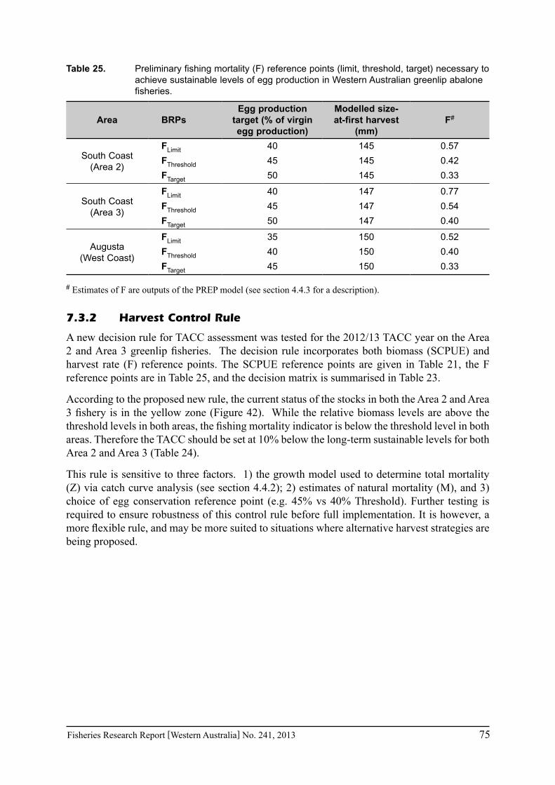
Fisheries Research Report [Western Australia] No. 241, 2013 75
Table 25. Preliminary fishing mortality (F) reference points (limit, threshold, target) necessary to achieve sustainable levels of egg production in Western Australian greenlip abalone fisheries.
Area BRPsEgg production
target (% of virgin egg production)
Modelled size-at-first harvest
(mm) F#
South Coast (Area 2)
FLimit 40 145 0.57
FThreshold 45 145 0.42
FTarget 50 145 0.33
South Coast (Area 3)
FLimit 40 147 0.77
FThreshold 45 147 0.54
FTarget 50 147 0.40
Augusta (West Coast)
FLimit 35 150 0.52
FThreshold 40 150 0.40
FTarget 45 150 0.33
# Estimates of F are outputs of the PREP model (see section 4.4.3 for a description).
7.3.2 Harvest Control Rule
A new decision rule for TACC assessment was tested for the 2012/13 TACC year on the Area 2andArea3greenlipfisheries. Thedecision rule incorporatesbothbiomass (SCPUE)andharvest rate (F) reference points. The SCPUE reference points are given in Table 21, the F reference points are in Table 25, and the decision matrix is summarised in Table 23.
According to the proposed new rule, the current status of the stocks in both the Area 2 and Area 3fisheryisintheyellowzone(Figure42). Whiletherelativebiomasslevelsareabovethethresholdlevelsinbothareas,thefishingmortalityindicatorisbelowthethresholdlevelinbothareas.ThereforetheTACCshouldbesetat10%belowthelong-termsustainablelevelsforbothArea 2 and Area 3 (Table 24).
This rule is sensitive to three factors. 1) the growth model used to determine total mortality (Z)viacatchcurveanalysis(seesection4.4.2);2)estimatesofnaturalmortality(M),and3)choiceof eggconservation referencepoint (e.g. 45%vs40%Threshold).Further testing isrequired to ensure robustness of this control rule before full implementation. It is however, a moreflexiblerule,andmaybemoresuitedtosituationswherealternativeharveststrategiesarebeing proposed.

76 Fisheries Research Report [Western Australia] No. 241, 2013
(A)
Biomass (SCPUE - 3yr mean)
9 10 11 12 13 14 15 16 17
Fis
hin
g m
ort
alit
y (F
)
0.2
0.3
0.4
0.5
0.6
0.7
04 05
07 08
09
10
11
FLIMIT
FTARGET
BTARGETBTHRESHOLDBLIMIT
(B)
Biomass (SCPUE - 3 yr mean)
9 10 11 12 13 14 15 16 17
Fis
hin
g M
ort
alit
y (F
)
0.2
0.3
0.4
0.5
0.6
0.7
04
05 06 07
08
09 10 11
FLIMIT
FTHRESHOLD
FTARGET
BTARGETBTHRESHOLDBLIMIT
Figure 42. Draft harvest control rules for the (A) Area 2, and (B) Area 3 greenlip fisheries based on the relationship between biomass (SCPUE) and fishing mortality (F) reference points (BRPs). The current status of the fishery is shown by the blue symbols (05 = 2005, 08 = 2008 etc.). TACC decision pertaining to the colour codes are summarised in Table 23.

Fisheries Research Report [Western Australia] No. 241, 2013 77
8.0 General Discussion
ThisreportpresentsthefirstcomprehensivesummaryofWesternAustralianabalonefisheries.Manyofthebiologicalparametershavenotpreviouslybeenpublishedandrepresentasignificantbodyofworkoveranumberofyears.Similarly,thetrenddatafromfisheryindependentsurveysinboththegreenlipandroe’sabalonefisherieshavenotpreviouslybeenavailableandsomevaluablefindingshavecome to light. Forexample, surveysof thePerthmetropolitan roe’sabalone stock have resulted in a predictive model for stock abundance. In the case of greenlip abalone,fisheryindependentsurveyssuggestthatstocklevelshavebeenstableoverthepast3 – 5 years.
The research into stunted greenlip stocks has clearly established the presence of ‘stunting’ in this species, both from an individual and a stock perspective. The correlation of growth and population surveydatahas enabledapracticaldefinitionof ‘stunting’ tobe applied infieldsurveys, and this has assisted the development of management strategies for these stocks. However, the research has also shown that growth and productivity of all greenlip stocks will lie somewhere in a large continuum from the very stunted, where maximum size reached is less than 120 mm, to the fast growing areas, where maximum size reached is greater than 180 mm. Size-at-maturity is similarly variable, ranging from 70 to 100 mm shell length.
Yield-per-recruit and egg-per-recruit analyses demonstrated that theArea 2 fisheries wereoptimallyexploitedwithrespecttoeggconservationtargets,howevertheArea3fisherieswouldbenefit fromminor reductions inminimumsizeoffishing.Furtherwork isneededon thesemodels, looking at effects of changes in growth, natural mortality, and fecundity parameters and also examining the value of different size abalone.
Environmentalinfluencesonabalonefisheriesabundancecontinuetobeimportant.Inthemostseverecase,theArea8roe’sabalonefisheryhasbeenwipedoutbyasingleeventofelevatedwater temperatures and associated deoxygenation of shallow waters. Further to this there may havebeensub-lethaleffectsintheArea7(Perthmetro)roe’sabalonefisheries,withpredictedstock levels of large animals (≥71 mm) not been achieved. Investigations are continuing and early signs suggest that the TACC and recreational catch quota for Area 7 may not be achieved inthe2012/13season.DespitethisstrongrecruitmentispredictedintheArea7fisherywithinthe next year or two, and a full recovery expected.
Development of performance indicators and TACC decision rules for Western Australian abalone fisheriesisamajorobjectiveachievedwiththisassessment.Theseruleshaveestablishedtheappropriate biological reference points for both stock biomass, and fishing mortality. Thereference points rely on fishery-independent and fishery-dependent survey information toensurestocklevelsarehighenoughforsustainablefishing.Useofdecisionrulesfacilitatesaresponsiveandflexiblemanagementregimecapableofaccommodatingeventssuchasalteringsize-at-harvest, or increasing recruitment with a stock enhancement program.
Overall,theassessmentsshowthatstocklevelsarecurrentlystableandfishingissustainable.Theeconomicperformanceofanychangesinfishingormanagementregimeshouldalsobeconsidered. The advantage of taking this adaptive management approach is that adequate performance indicators and TACC decision rules are now in place. These will monitor the responseofthefisherytoanychangesinfishingormanagementregimeandadjustcatchquotasaccordingly.

78 Fisheries Research Report [Western Australia] No. 241, 2013
9.0 Recommendations for future research
• Investigation of the basic biology of brownlip abalone, such as studies of growth and natural mortality.
• Further analysis on yield and egg-per recruit models to optimise growth, natural mortality, and fecundity parameters
• Examine catch variability in the Perth recreational roe’s ablone fishery as a function ofindividual ‘weather condition’ factors such as swell, tide, wind, rainfall, and cloud cover.
• DevelopmentofapopulationdynamicsmodelsforWesternAustralianabalonefisheriesthatenable formal evaluations of appropriate harvest levels.
• Bioeconomic evaluations of fishing policy, including economic yield-per-recruit, andassessmentofincreasesinNPV(NetPresentValue)underdifferentharvestscenarios.
• Develop catch predictions
• Consider environmental factors affecting recruitment and evaluate the effects of climate change.
Fisheries Research Report [Western Australia] No. 241, 2013 79
10.0 ReferencesAndrew NL, Chen Y (1997). Optimal sampling for estimating the size structure and mean size of abalone
caughtinaNewSouthWalesfishery.Fishery Bulletin 95 (3): 403-413.
BaranovFI(1918).Onthequestionofthebiologicalbasisoffisheries.Nauchn.Issled.Ikhtiol.Inst.Izv.1: 81-128. [In Russian].
ClarkWG(2002).F35%revisitedtenyearslater.North American Journal of Fisheries Management. 22(1): 251–257.
Daume S, Brand-Gardner S, and Woelkerling WJ (1999). Preferential settlement of abalone larvae: diatomfilmsvs.non-geniculatecorallineredalgae.Aquaculture, 174: 243-254.
GorfineH,ForbesDA,GasonAS(1998).Acomparisonoftwounderwatercensusmethodsforestimatingtheabundance of the commercially important blacklip abalone, Haliotis rubra. Fishery Bulletin, 96: 438-450
Hancock B (2004). The biology and fishery of Roe’s abaloneHaliotis roei Gray in south-western Australia,withemphasisonthePerthfishery.PhDthesis,UniversityofWesternAustralia.184p
HancockB,CaputiN (2006).TheRoe’s abalone fishery near the Perthmetropolitan area,WesternAustralia. Journal of Shellfish Research 25(1), 167-178
Hart AM., LWS Strain, FP Fabris, J Brown, and M. Davidson (in press a) Stock enhancement in greenlip abalone: (1) Long-term growth and survival. Reviews in Fisheries Science.
Hart, AM, FP Fabris, LWS Strain, M Davidson, and J Brown (in press b). Stock enhancement in greenlip abalone: (2) Population and ecological effects. Reviews in Fisheries Science.
Hart, A M, LWS Strain, A. Hesp (in press c). Stock enhancement in greenlip abalone: (3) Bioeconomic evaluation. Reviews in Fisheries Science
Hart AM, Fabris FP, Baharthah, T. 2010. Greenlip Brownlip Abalone Fishery status report. In: State of the Fisheries Report 2009/10, eds W.J. Fletcher and K. Santoro, Department of Fisheries, Western Australia, pp. 221-228.
Hart AM, Fabris FP, Caputi N (2009). Performance indicators, biological reference points, and decision rules forWesternAustralian abalone fisheries (Haliotis sp.): Standardised catch per unit effort. Fisheries Research Report No 185, Department of Fisheries, Western Australia, 40 p
Hart AM, Fabris FP, Brown J, Murphy D (2008). Digital video surveys of abalone (Haliotis sp.) stocks bycommercialfishersinWesternAustralia.Fisheries Research. 93: 305-314
Hart AM, Fabris FP, Daume S (2007). Stock enhancement of Haliotis laevigata in Western Australia - a preliminary assessment. Fisheries Research Report No 166, Department of Fisheries, Western Australia, 40 p
Hart AM, Syers C, Hall N (2000). Stock assessment and modeling for management of the WA greenlip abalonefishery.FinalReporttoFisheriesResearchandDevelopmentCorporation.ProjectNo:95/143
HartAM,GorfineHK,CallanMP(1997).Abundanceestimationofblacklipabalone(Haliotis rubra) I. An analysis of diver-survey methods used for large-scale monitoring. Fisheries Research, 29: 159-169.
Hesp A, Loneragan N, Hall N, Kobryn H, Hart AM, Fabris FP, Prince J (2008). Biomass and commercial catch estimates for abalone stocks in areas proposed as sanctuary zones for the Capes Marine Park. Fisheries Research Report No 170, Department of Fisheries, Western Australia, 62 p
Keesing J (1984). Reproductive biology of the abalone Haliotis roei Gray, 1827, in south-western Australia. Honours Thesis. Murdoch University, Western Australia. 99 pp
Lindberg DR (1992). Evolution, distribution, and systematics of Haliotidae. In Abalone of the World: Biology, Fisheries, and Culture (Eds: SA Shepherd, MJ Tegner, SA Guzman Del Proo). Fishing NewsBooks,BlackwellScientific,London.
MayfieldS,MundyC,GorfineH,HartAM,&D.Worthington(2012).FiftyyearsofsustainedproductionfromtheAustralianabalonefisheries.Reviews in Fisheries Science, 24: 220-250

80 Fisheries Research Report [Western Australia] No. 241, 2013
MayfieldS,SaundersT(2008).Towardsoptimisingthespatialscaleofabalonefisherymanagement.SARDI Research Report Series no. 273, SARDI, South Australia, 148 p.
MayfieldS,FoureurBL,RoddaKR,PreecePA,WardTM(2003).WesternZoneAbalone(Haliotis laevigata &H. rubra) Fishery 1, Region A: Fishery Assessment Report to PIRSA Fisheries. SARDI, South Australia.
McAveney LA, Day RW, Dixon CD, Huchette SM (2004). Gonad development in seeded Haliotis laevigata: growth environment determines initial reproductive investment. Journal of Shellfish Research. 23 (4): 1213-1218.
McShanePE(1995).Recruitmentvariationinabalone:Itsimportancetofisheriesmanagement.Marine and Freshwater Research, 46: 555-530.
McShane PE (1992). Early life history of abalone: a review. In Abalone of the World: Biology, Fisheries, and Culture (Eds: SA Shepherd, MJ Tegner, SA Guzman Del Proo). Fishing News Books, Blackwell Scientific,London
OfficerRA,SizelimitsforgreenlipabaloneinTasmania.TAFITechnicalReportSeriesNo.5.TasmanianAquaculture and Fisheries Institute. 48 p.
Pauly D (1984). Fish population dynamics in tropical waters: A manual for use with programmable calculators: ICLARM Studies and Reviews 8, 325 p. International Center for Living Aquatic Resources Management.
PearceA,LenantonR,JacksonG,MooreJ,FengM,GaughanD(2011).The“marineheatwave”offWestern Australia during the summer of 2010/11. Fisheries Research Report No 222, Department of Fisheries, Western Australia, 40 pp.
PrinceJD,PeetersH,GorfineH,DayRW.Thenoveluseofharvestpoliciesandrapidvisualassessmentto manage spatially complex abalone resources (Genus Haliotis). Fisheries Research. 94: 330-338.
SaundersT,MayfieldS,HoggA(2009).Usingasimplemorphometricmarkertoidentifyspatialunitsforabalonefisherymanagement.ICES Journal of Marine Science, 66: 305-314.
Shepherd SA, Baker JL. Biological reference points in an abalone (Haliotis laevigata)fishery.1998.Canadian Special Publications in Fisheries and Aquatic Science, 125: 235-245.
Shepherd SA, Hearn WG. Studies on southern Australian abalone (Genus Haliotis):IV.GrowthofH. laevigata and H. ruber. Australian Journal of Marine and Freshwater Research, 34: 461-475.
Shepherd SA, Steinberg PD (1992). Food preferences of three Australian abalone species with a review of the algal food of abalone. In Abalone of the World: Biology, Fisheries, and Culture (Eds: SA Shepherd,MJTegner,SAGuzmanDelProo).FishingNewsBooks,BlackwellScientific,London
TarbathF,OfficerR (2003). Size limits and yield for blacklip abalone in northernTasmania.TAFITechnical Report Series No. 17. Tasmanian Aquaculture and Fisheries Institute. 37 p.
Wells FE, Mulvay P (1995). Good and bad fishing areas forHaliotis laevigata: A comparison of population parameters. Marine and Freshwater Research: 46, 591-598.
Wells FE, Mulvay P (1992). Reproduction and growth of the greenlip abalone Haliotis laevigata on the south coast of Western Australia. Unpublished report to the Western Australian Department of Fisheries.117 pp
Worthington DG, Andrew NL (1997). Does covariation between growth and reproduction compromise the use of an alternative size limit for the blacklip abalone, Haliotis rubra, in NSW, Australia. Fisheries Research. 32: 223-231.
Worthington DG, Andrew NL, Hamer G (1995). Covariation between growth and morphology suggests alternative size limits for the blacklip abalone, Haliotis rubra, in New South Wales, Australia. Fishery Bulletin. 93: 551 - 561
ZhouS,YinS,ThorsonJT,SmithADM,FullerM(2012).Linkingfishingmortalityreferencepointstolifehistory traits: an empirical study. Canadian Journal of Fisheries and Aquatic Science. 69: 1292 - 1301

Fisheries Research Report [Western Australia] No. 241, 2013 81
11.0 Appendices
11.1 Performance indicators and biological reference points for each management area and species
11.1.1 Area 1 Greenlip and Roe’s abalone fishery
Area 1 is remote and inaccessible, being principally stationed below the Nullabor Cliffs (see Figs.2&3)andfishingisgenerallyofanexploratorynature.Consequently,thehistoricaltimeseries of catch per unit effort for both Greenlip and Roe’s abalone was too variable to be used to develop PI’s. TAC assessment and management in this region will continue to be based largely on raw data trends and feedback from industry divers as to their own harvest plans.
11.1.2 Area 2 Roe’s abalone fishery

82 Fisheries Research Report [Western Australia] No. 241, 2013
11.1.3 Area 2 Greenlip abalone fishery
11.1.4 Area 3 Greenlip abalone fishery
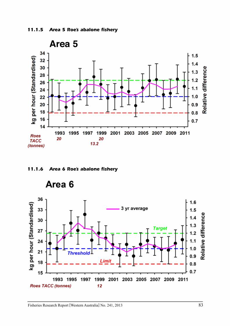
Fisheries Research Report [Western Australia] No. 241, 2013 83
11.1.5 Area 5 Roe’s abalone fishery
11.1.6 Area 6 Roe’s abalone fishery
Area 5

84 Fisheries Research Report [Western Australia] No. 241, 2013
11.1.7 Area 7 Roe’s abalone fishery
11.1.8 Area 8 Roe’s abalone fishery
Area 7

Fisheries Research Report [Western Australia] No. 241, 2013 85
11.2 Catch and Effort maps
These maps show spatial scale (10 x 10 nautical mile grids) at which catch and effort information isrecordedforthecommercialabalonefishery.

86 Fisheries Research Report [Western Australia] No. 241, 2013
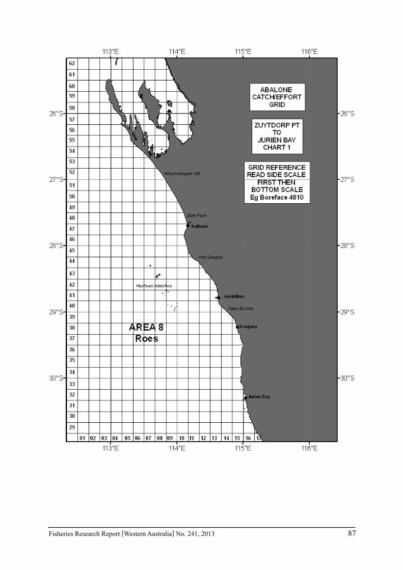
Fisheries Research Report [Western Australia] No. 241, 2013 87

88 Fisheries Research Report [Western Australia] No. 241, 2013

Fisheries Research Report [Western Australia] No. 241, 2013 89

90 Fisheries Research Report [Western Australia] No. 241, 2013