Journal of Ecology

2003

91

, 757–775

© 2003 British Ecological Society

Blackwell Publishing Ltd.

Habitat association among Amazonian tree species: a landscape-scale approach

OLIVER L. PHILLIPS, PERCY NÚÑEZ VARGAS†‡, ABEL LORENZO MONTEAGUDO‡, ANTONIO PEÑA CRUZ§, MARIA-ELENA CHUSPE ZANS‡, WASHINGTON GALIANO SÁNCHEZ‡, MARKKU YLI-HALLA¶ and SAM ROSE*

School of Geography, Earth and Biosphere Institute, University of Leeds, Leeds, UK,

†

Biodiversidad Amazónico, Cusco, Peru,

‡

Herbario Vargas, Universidad Nacional, San Antonio Abad del Cusco, Peru,

§

Jardin Botánico de Missouri, Oxapampa, Peru, and

¶

MTT, Agrifood Research Finland, Jokioinen, Finland

Summary

1

Unravelling which factors affect where tropical trees grow is an important goal forecologists and conservationists. At the landscape scale, debate is mostly focused on thedegree to which the distributions of tree species are determined by soil conditions or byneutral, distance-dependent processes. Problems with spatial autocorrelation, sparsesoil sampling, inclusion of species-poor sites with extreme edaphic conditions, and thedifficulty of obtaining sufficient sample sizes have all complicated assessments for highdiversity tropical forests.

2

We evaluated the extent and pervasiveness of habitat association of trees within a10 000 km

2

species-rich lowland landscape of uniform climate in south-west Amazonia.Forests growing on two non-flooded landscape units were inventoried using 88 floristicplots and detailed soil analyses, sampling up to 849 tree species. We applied single-species and community-level analytical techniques (frequency-distributions of presencerecords, association analysis, indicator species analysis, ordination, Mantel correlations,and multiple regression of distance matrices) to quantify soil/floristic relationshipswhile controlling for spatial autocorrelation.

3

Obligate habitat-restriction is very rare: among 230 tree species recorded in

≥

10localities only five (2.2%) were always restricted to one landscape unit or the other.

4

However, many species show a significant tendency to habitat association. For exam-ple, using Monte Carlo randomization tests, of the 34 most dominant species across thelandscape the distributions of 26 (76.5%) are significantly related to habitat. We applieddensity-independent and frequency-independent estimates of habitat association andfound that rarer species tend to score higher, suggesting that our full community estimates ofhabitat association are still underestimated due to the inadequate sampling of rarer species.

5

Community-level floristic variation across the whole landscape is related to thevariation in 14 of 16 measured soil variables, and to the geographical distances betweensamples.

6

Multiple regression of distance matrices shows that 10% of the floristic variation canbe attributed to spatial autocorrelation, but even after accounting for this at least 40%is attributable to measured environmental variation.

7

Our results suggest that substrate-mediated local processes play a much moreimportant role than distance-dependent processes in structuring forest composition inAmazonian landscapes.

Key-words

: forest, floristics, soils, spatial autocorrelation, tree species composition.

Journal of Ecology

(2003)

91

, 757–775

Correspondence: Oliver Phillips, School of Geography, Earth and Biosphere Institute, University of Leeds, Leeds LS2 9JT, UK(e-mail o.phillips@geog.leeds.ac.uk).*Present address: Volunteer Services Overseas, London, UK.

758

O. L. Phillips

et al.

© 2003 British Ecological Society,

Journal of Ecology

,

91

, 757–775

Introduction

A fundamental goal of plant ecology is to understandthe relative importance of the environment and ofchance in structuring plant communities. Tropical for-ests include the earth’s most diverse communities, andniche differentiation with respect to resources is fre-quently invoked as a means by which this exceptionaldiversity is maintained (e.g. Grubb 1977; Denslow1987). Several studies have demonstrated demographicpatterns and life-history variation along successionallight-intensity gradients that may help explain coexist-ence of tropical tree species (e.g. Clark & Clark 1992;Condit

et al

. 1996; Condit

et al

. 1999; Rees

et al

. 2001).However, the extent to which tropical trees specializewith respect to edaphically and topographically deter-mined resources – such as soil nutrients and moistureavailability – is the subject of an especially persistentand vigorous debate. Some studies have found nostrong effect of soil conditions on lowland tropical treefloristic patterning (e.g. Poore 1968; Wong & Whitmore1970; Knight 1975; Newbery & Proctor 1983; Hubbell& Foster 1986; Newbery

et al

. 1988; Hart

et al

. 1989;Pitman

et al

. 1999). Where researchers have reportedthat the floristic composition of tropical lowlands res-ponds to edaphic differences, the studies rarely allowus to draw general conclusions about the degree ofhabitat association in tree species across species-richtropical landscapes.

The large practical difficulties inherent in collectingand identifying thousands of non-fertile collectionsrepresenting hundreds of species in poorly mappedlandscapes have encouraged researchers to developalternative approaches. Thus, for example, studies haveoften focused on family level patterns (e.g. Gentry1988a; Terborgh & Andresen 1998; ter Steege

et al

.2000), the impact of extreme soil conditions (such aswhite-sand podsols, floodplain entisols, swamp his-tosols, or limestone mollisols, e.g. Newbery & Proctor1983; Kalliola

et al

. 1991; Vásquez & Phillips 2000, andcf. Sollins 1998), the importance of microhabitat topo-graphic variation (e.g. Sabatier

et al

. 1997; Svenning1999; Vormisto

et al

. 2000), relatively depauperateregions (e.g. Swaine 1996), distributions of particulartree taxa (e.g. Debski

et al

. 2002) or particular non-treeelements of the flora (e.g. Clark

et al

. 1995; Poulsen1996; Fleck & Harder 2000; Tuomisto & Poulsen 2000;Tuomisto

et al

. 2003a,b), or do not make allowancefor spatial aggregation of species’ populations, a near-ubiquitous feature of tropical forests (cf. Condit

et al

.2000).

Recently it has been shown that the importance offactors such as habitat variation in structuring tropicalforest communities may vary greatly with scale andlocality (Condit

et al

. 2002). This implies that ourunderstanding of tropical community pattern andprocess is heavily influenced by the geography of eco-logical research, which is typically done at small scalesin a limited number of localities. In the Neotropics, for

example, the intensity of research in Central Americanforests outscores that in Amazonian forests by a factorof > 50 on a per area basis (based on a survey of ISIpublications between January 2000 and June 2002reporting primary ecological research from Panama,Costa Rica and Amazonia). Most studies that doclearly demonstrate substrate-mediated habitat asso-ciation in tropical tree species are central American(e.g. Clark

et al

. 1998, 1999; Condit

et al

. 2000, 2002;Harms

et al

. 2001; Pyke

et al

. 2001; Faith & Ferrier2002). In Amazonia, encompassing more than half theworld’s lowland rain forest, the importance of species’habitat associations in controlling community diver-sity and composition remains particularly contentious(e.g. Salo

et al

. 1986; Gentry 1988a; ter Steege

et al

.1993; Duivenvoorden 1995; Tuomisto

et al

. 1995;Ruokolainen

et al

. 1997; Pitman

et al

. 1999; Condit

et al

. 2002). According to one view, large areas of theAmazon feature low beta-diversity and a substantiallyhomogeneous flora. Pitman

et al

. (2001), for example,have shown that a similar set of tree species dominatesAndean foreland landscapes > 10

3

km apart in Peru andEcuador. Alternatively, the appearance of homogeneitycould be exaggerated by the difficulty in musteringsufficient statistical power to detect heterogeneity inspecies distributions within landscapes (Ruokolainen

et al

. 1997).Western Amazonia supports the world’s most tree

species-rich forests (e.g. Gentry 1988b) and the scarcertaxa that may be the most important for conservationare also the most difficult to characterize environmen-tally. With some important exceptions (e.g. Tuomisto

et al

. 1995; Kalliola

et al

. 1998) vegetation mapping inAmazonia has produced relatively uniform results,with only a handful of different environmentally deter-mined vegetation formations broadly controlled byregional climatic and geomorphological features (e.g.UNESCO 1980; Sombroek 2001). Can these maps berelied on to reflect floristically defined communities, oris the floristic composition of forests a more finelygrained affair, with distributions substantially medi-ated by localized soil formations? The question is notonly important for plant ecologists but also for land-use planners and conservationists who need reliablevegetation maps to help identify forest communitiesand species at particular risk.

A few edaphically and hydrologically determinedvegetation types

are

recognized within lowland Ama-zonia, particularly palm swamps, floodplain forests,and forests on podzolized white sand soils (e.g.Anderson 1981; Pires & Prance 1985; Kahn & Mejia1990; Duque

et al

. 2002), but these occupy minor areascompared with the unflooded forest on non-podzolizedsoil, so-called ‘terra firme’ forest, which covers themajority of lowland Amazonia (UNESCO 1980). Ethno-botanical evidence (Fleck & Harder 2000; Shephard

et al.

2001; Shephard

et al.

2003) shows that indigenouspeople recognize numerous distinct habitats withinterra firme, characterized by congruous variation in

759

Habitat association of Amazon trees

© 2003 British Ecological Society,

Journal of Ecology

,

91

, 757–775

soil, topography, vegetation structure, and character-istic species of flora and fauna, indicating that currentacademic understanding of the floristic landscape isstill inadequate. Ecologists’ attempts to characterizetree species variation across whole Amazonian land-scapes are hampered by the difficulty of achieving suf-ficient sampling within individual sampling units whilealso realizing spatial replication across the landscape.Both features can generate high sampling error, andthis renders it difficult to identify the signal of floristicpatterns in floras of 1000 tree species or more. Forexample, Pitman

et al

. (1999) and Condit

et al

. (2002)sampled at least 19 000 Amazonian trees, but the lim-ited soil data and small number of discrete sample plotsmay make detecting species-level habitat associationdifficult; Duivenvoorden (1995) used more plots (95)but sampled fewer stems. These studies concludedthat species turnover from one substrate to another(

β

−

diversity) is low in non-flooded forests.Here we bring a new, large single-landscape Amazon

ecofloristic data set to bear on the question of theextent to which tree species distributions are deter-mined by edaphic factors within a tropical landscape.Specifically, we ask: (i) What proportion of species arecompletely confined to different terra firme habitats?(ii) Is a tendency to habitat association limited to a fewindividual species, or is it a widespread property of theAmazonian flora? (iii) Is habitat association of speciesindependent of measures of ecological success suchas density and frequency? (iv) What is the relativeimportance of stochastic and environmental factors incontrolling floristic patterns across an Amazonianlandscape? Each question was asked for all sampledspecies attaining a stem diameter of

≥

2.5 cm, and thenfor the subset of species that attain a diameter of

≥

10 cm.

Methods

Our study area in Madre de Dios, south-eastern Peru,was defined as a rectangle with

c

. 100 km edges, centredon the town of Puerto Maldonado. The region is still> 90% forested and is dominated by past (Pleistoceneto Holocene) and present fluvial activity (Räsänen

et al

. 1992).

Sampling approach

The region has near uniform elevation (200–260m a.m.s.l) and a seasonal tropical climate, with meanannual rainfall of 2200–2400 mm, 3 months a yearaveraging less than 100 mm, and a mean annualtemperature of > 25

°

C (Duellman & Koechlin 1991;Malhi

et al

. 2002).Forests are found on three distinct geomorphological

units (Salo

et al

. 1986; Räsänen

et al

. 1990, 1991, 1992;Salo & Kalliola 1990; Osher & Buol 1998): irregularly

flooded areas of the contemporary floodplains of theTambopata, Heath, Las Piedras and Madre de Diosrivers (

c

. 9% of the study area), no-longer floodedterraces of the Holocene floodplain of these rivers(

c

. 20%), and ancient Pleistocene alluvial terraces atleast 40 000 years old (58%). Swamp forests are foundin small histosol patches within each unit, particularlythe contemporary floodplains, but most forest (89%)grows on better drained ultisols that dominate thePleistocene surfaces (Osher & Buol 1998) or inceptisolsand ultisols on the Holocene surface (Malhi

et al

.2004). Samples were located in old-growth forests in 13community territories and protected areas (Fig. 1,Appendix 1 and 2 in Supplementary Material), stratifiedby geomorphology on the basis of visual assessment ofa Landsat image (path 002 row 069) ground-truthedover a 2-year period by checking relative topographicalpositions and detailed mapping with local residents.Our focus here is on patterns within the ultisols andinceptisols of the terra firme forests, so we deliberatelyexclude all samples in swamp forests and contem-porary floodplains from the analysis. The region lacksother important and distinctive tropical soils, such ashighly weathered oxisols or white sand soils (spodosols),or those derived from basaltic, volcanic ash, limestoneor serpentine substrates. Therefore, our approachprovides a rather conservative evaluation of the extentof species association within mature tropical forests,and even within mature unflooded tropical forests.Holocene and Pleistocene surfaces are well distributedthroughout, so by sampling both surfaces across thelandscape we aimed to disentangle the roles of spatialand environmental factors.

Sample units

Our approach is a modification of an inventoryapproach first used extensively in tropical forests byGentry (e.g. Gentry 1982, 1988a; Enquist & Niklas2001; Phillips & Miller 2002; Phillips

et al

. 2003). For-ests at each location were sampled in 1998 and 1999 by10 2

×

50 m subplots, totalling 0.1 ha, and locatedwithin a 100

×

180 m sampling grid so as to systema-tically subsample 1.8 ha of forest. Each non-scandentplant rooted within the transect area and with a stemdiameter of

≥

2.5 cm at 1.30 m height (= diameter atbreast height, d.b.h) was included in the sample, andevery plant measured and identified or recorded asa unique ‘morphospecies’. Voucher collections weremade for each unique species and whenever there wasany uncertainty to its identity. Repeated collectionsof sterile plants were frequently needed to reliably dis-tinguish morphospecies. A full set of duplicates isdeposited in Peru at CUZ, where vouchers wereidentified and cross-referenced. A partial set is alsomaintained at USM.

We collected soil samples (0–15 cm below the organicmaterial layer) from each inventory location by augur-ing each of the 2

×

50 subplots at one or more randomly

760

O. L. Phillips

et al.

© 2003 British Ecological Society,

Journal of Ecology

,

91

, 757–775

chosen points and then bulking the subsamples foreach inventory. Composite samples were air-dried,cleaned by removing macroscopic organic material,and subsampled. Drainage conditions were assessedvisually on a scale of 1 (permanently water-logged) to10 (excessively drained) for each subplot and meanvalues derived for each inventory. Chemical and phys-ical soil properties were analysed at the AgriculturalResearch Center in Finland following ISRIC protocols(Van Reeuwijk 1995): soil pH was measured in a 1-

KCl suspension; exchangeable Ca, Mg, K and Nawere extracted with 1

ammonium acetate (pH 7.0);exchangeable Al was extracted with 1

KCl; plant-available P was determined by the Bray 1 method (0.03

NH

4

F

−

0.025

HCl extraction); clay (< 2

µ

m), silt(2–63

µ

m) and sand (0.63–2 mm) content was deter-mined after pre-treatment with citrate – dithionite –bicarbonate; and loss of weight on ignition (LOI) wasdetermined by heating the dried soils at 420

°

C for6 h. Effective cation exchange capacity (ECEC) wascalculated as the sum of cation charge, expressed incmol(+) kg

−

1

.

Eighty-eight mature forest samples were includedin the data set. All records of unidentified morpho-species were removed to eliminate the possibility thatinconsistent cross-referencing of vouchers within and

between communities might bias the results. Eachspecies in this data set was checked for maximum dia-meter within the 88

×

0.1-ha samples and against anindependent data set of trees in 16

×

1.0-ha per-manent sample plots in eastern Madre de Dios (Gentry1988a; Phillips

et al

. 1998, Phillips, Vásquez Núñez, &Monteagudo, unpublished data) to identify the plantsthat attain

≥

10 cm stem diameter as self-supportingadults. Analyses that follow were applied both to species

≥

10 cm d.b.h. (‘trees’), and to all species

≥

2.5 cmd.b.h. in our data set.

We evaluate habitat association within terra firmeforests using two distinct approaches. In the first,we simply divide our samples into Holocene andPleistocene surfaces and examine the extent to whichindividual species are generally confined to one orother landscape unit. In the second approach, we exam-ine the extent to which the entire floristic compositionof forests varies with both physical and spatial factors,using ordination, Mantel tests, and multiple regressionon distance matrices.

Treatment of spatial autocorrelation

Patterns of habitat association can be confounded byspatial autocorrelation, as geographically proximatesamples are more likely to share species due to stochas-tic processes than geographically distant samples (e.g.Condit

et al

. 2000; Harms

et al

. 2001). Our analyses

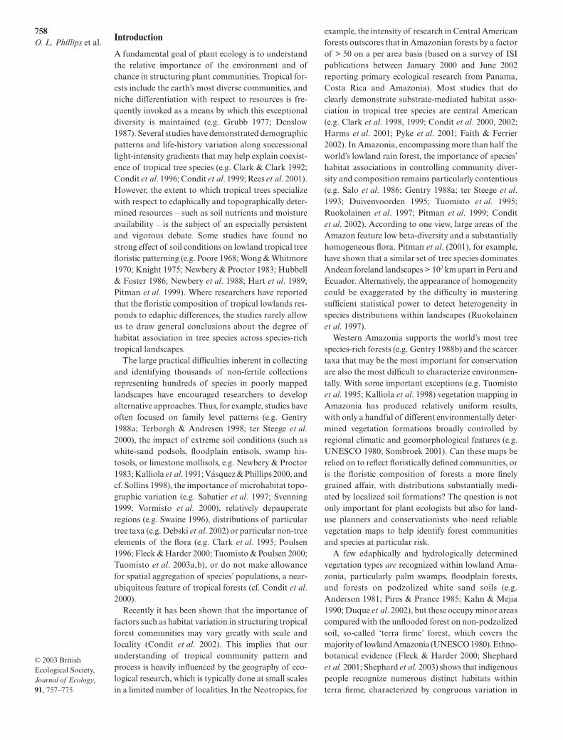
Fig. 1 Map of study area showing distribution of sample locations. Closed circles represent Holocene samples; open circlesrepresent Pleistocene samples. All samples are located between 12° S and 13° S and 68°30′ W and 69°30′ W.

761

Habitat association of Amazon trees

© 2003 British Ecological Society,

Journal of Ecology

,

91

, 757–775

either specifically parcel out and quantify the com-ponents of floristic variation potentially due to spatialautocorrelation and due to environmental attributes(cf. Condit

et al

. 2002), or use permutation proceduresto compare patterns against null expectations gener-ated by hypotheses of no habitat effect. Traditional chi-squared association analysis of density patterns is alsoused for comparison.

1

:

First, we examine whether species are sampled in onlyone habitat (‘narrowly restricted’, following Pitman

et al

. 1999), or not (‘widespread’). By this definition theprobability of a species appearing to be ‘narrowlyrestricted’ will vary artifactually as an inverse functionof the frequency with which it is encountered, so wecompare the empirically observed pattern with a nullexpectation of frequency distributions generated by abinomial distribution assuming no habitat restriction.This is the simplest technique for evaluating habitatassociation, as it takes account of presence/absencedata but makes no allowance for differences in relativedensities between habitats. Secondly, we relax the testof habitat association from ‘narrow restriction’ to ‘tend-ency’. To assess the tendency with which species arefavoured by one habitat or another we compare foreach species both their frequency-distribution patternsand density-distribution patterns against null expecta-tions, and evaluate overall differences in speciesfrequencies and densities between habitats using chi-squared tests of association. Thirdly, we use indicatorspecies analysis (Dufrene & Legendre 1997) to accountfor both relative abundance and relative frequency ofeach species across the landscape, by testing the degreeof habitat association at the level of species againstindividually parameterized null models.

The null hypothesis is that the highest indicatorvalue for each species in one or other habitat (

IVmax

)is no larger than would be expected if the species wasdistributed at random across the two landscape units.Significance is estimated by a Monte Carlo procedurethat reassigns species densities and frequencies tohabitats 1000 times. The probability of type I error isbased on the proportion of times that the

IVmax

scorefor each species from the randomized data set equalsor exceeds its

IVmax

score from the actual data set(McCune & Mefford 1999). Finally, to address thequestion of whether habitat association is associatedwith species density in the landscape we developedsimple density- and frequency-independent indices ofhabitat association for each species, based on therelative difference between the probability of beingencountered in Pleistocene samples and Holocenesamples, and we relate both these indices and

IVmax

scores to species density values.Thus, the density-independent index of habitat

association,

A

Dx

= the absolute value of {(PD)/(PD + HD) − (HD)/ (PD + HD)}

where, for each species x:

(PD) = the density of that species in the Pleistocene samples;

(HD) = the density of that species in the Holocene samples.

ADx varies between 0 (= no habitat association with equal density in each landscape) and 1 (= every stem of that species found in one habitat or the other).

Similarly, the frequency-independent index of habitatassociation,

AFx = the absolute value of {(PF)/(PF + HF) − (HF)/ (PF + HF)}

where, for each species x:

(PF) = the frequency of that species in the Pleistocene samples;

(HF) = the frequency of that species in the Holocene samples.

AFx varies between 0 (= no habitat association) and 1 (= every record of that species being from samples in one habitat or the other).

We used the entire data set for the first and second setof analyses, following established practice. However,we needed to eliminate the possibility of spatial auto-correlation affecting our other analyses (the indicatorspecies analysis, and calculations of density-independentand frequency-independent habitat association scores).Our procedure was as follows. First, we examined atwhat spatial scale within-habitat sample clusteringoccurred (i.e. over what intersample pair distances wasthere a greater than expected probability of both sam-ples representing the same habitat). Over intersampledistances of < c. 5000 m and especially < c. 1500 msample pairs are more likely than not to representthe same habitat. Then, we determined the number ofwithin-habitat pairwise combinations that had to beeliminated to bring the odds to 1 in 2 of a random sam-ple pair being from the same habitat over all distances< 5000 m. Finally, we progressively removed samplesfrom the data base, starting with the shortest distanceof same-habitat sample pairs; for each sample pair weselected the one sample that also had the secondnearest same-habitat neighbour. In practice there arefew samples very close to one another (of 3829 poten-tial pairwise combinations, only 14 have distances< 1000 m), so the removal of relatively few samplesfrom the data set (nine out of 88) eliminates the prob-lem. Of the original 38 Holocene samples we needed toremove five (LAT7, PNB1, PTA9, SAB9 and SAB10);

762O. L. Phillips et al.

© 2003 British Ecological Society, Journal of Ecology, 91, 757–775

of the original 50 Pleistocene samples we needed toremove four (BOC5, PTA5, PTA6 and SJC3).

2 :

Construction of distance matrices

We explore potential relationships between plantspecies composition and soil on the basis of site-to-sitecomparisons. Distance between all possible pairs ofsites was measured for each of three classes of variable– (i) plant species composition, (ii) each of 15 soilvariables, and (iii) geographical distance among thesites – to produce a dissimilarity matrix between allpossible sample-pairs for all variables.

We measured floristic distance between sample pairsusing the Sørensen (Bray-Curtis) index of similarity,widely used in community analyses because it retainssensitivity to the data structure without giving undueweight to outliers (e.g. Ludwig & Reynolds 1988). Dis-tance matrices on the basis of soil characteristics (Ca,K, Mg, Na, sum of base cations, Al, ECEC, Al/ECEC,P, pH, LOI, sand, silt, clay, fraction < 0.063 mm), andgeographical distances are based on Euclidean dis-tance, i.e. the difference in the values of the each samplepair. Before calculating distances we transformed vari-ables using Tukey’s ladder of powers (Table 1); thiscorrected positively skewed distributions and ensuresthat absolute differences between low values receivegreater analytical weight than differences between highvalues. This treatment is more likely to reflect environ-mental and spatial differences experienced by plantsthan would non-transformation of raw variables. Forexample, Hubbell’s (2001) neutral theory predictsnon-linear distance decay in similarity, and Conditet al. (2000, 2002) have shown this result empirically intropical forest landscapes.

Analyses using the distance matrices

We used the distance matrices in four different ana-lyses: first, by plots of sample-pair similarity against dis-tance to quantify spatial decay; secondly, a non-metricmultidimensional distance scaling ordination (NMDS,Kruskal 1964) to explore the compositional patterns;thirdly, Mantel’s test on matrix correlation (Mantel1967) to test for interdependence among key variables;and finally, multiple regression on distance matrices(Legendre et al. 1994), to model the full floristic vari-ation in terms of the spatial and environmental factors.

NMDS is an ordination method that arranges thesamples in a user-defined limited number of dimen-sions so that the rank order of distances is as similar aspossible to the rank order in the original data. Thesolution is found iteratively to find the best number k ofdimensions for a given data matrix. We used the pro-gram PC-ORD for producing the NMDS ordinations,running 400 iterations each starting with a randomconfiguration, adopting k = 6, and applying an insta-bility criterion of 10−5. The Mantel test involves com-puting the Pearson correlation coefficient between thevalues of two matrices (Smouse et al. 1986), and usinga Monte Carlo procedure to estimate the probability oferror. We distinguished a 0.1% probability of error bycomparing observed distributions of r against the dis-tribution of random values generated from permutingone of the matrices and recalculating r 999 times. Apartial Mantel test was used to evaluate how correla-tions between floristic composition and environmentalvariables changed after controlling for the effect of geo-graphical distance. The Mantel tests were performedwith PC-ORD and with the R-Package (Legendre &Vaudor 1991) for all pairwise variable combinations.

In the multiple regression method on distance matri-ces the variation in one dependent matrix is expressedin terms of variation in a set of independent matrices.The computational procedure mimics that of normalmultiple regression, except that the significance ofparameters is estimated by the Monte Carlo permuta-tion procedure described above (Legendre et al. 1994).We developed models to describe the variation of thefloristic data set in terms of environmental and spatialfactors, by undertaking a multiple regression of the flo-ristics distance matrix against the variable distancematrices. Both forward selection and backwards elim-ination methods were used. Here our aim is to ascertainthe contribution of environmental factors to floristicpattern within the terra firme landscape, havingaccounted for the spatial fraction. The three-stagemodel generation and selection procedure reflects this:(i) we built the largest model possible in which eachfactor contributes significantly (at P = 0.01); (ii) weeliminated independent variables with negative b-coefficients, until all remaining b-coefficients werepositive (negative b-coefficients are not interpretableas they imply that as values of environmental variablesin samples become closer the differences in species

Table 1 Soil and Distance variable transformations

Variable Transformation

pH –(x − 3.2)−1

Ca ln(x)K ln(x)Mg log10(x)Na –x−0.5

Al x−2

ECEC –x−0.5

Al/ECEC xP –x−0.5

Dry matter (x − 89.5)3

Loss on ignition –x−0.5

Sand x−2

Silt x2

Clay ln(x)Fraction < 0.063 mm xMean drainage x2

Geographical distance ln(x)

763Habitat association of Amazon trees

© 2003 British Ecological Society, Journal of Ecology, 91, 757–775

composition between them become greater); finally(iii), we applied backward elimination with Bonferronicorrected probability levels (estimated on the basis of999 permutations) to decide eliminations, holding theintersite spatial distance matrix as the last factor to beexcluded so that we could differentiate all floristicvariation that had a spatial structure. The procedurewas conducted first for the whole data set, and variablesin the best all-species model were evaluated for treespecies in order to be able to compare the two data setsdirectly. All multiple regressions on distance matriceswere performed with the Permute! 3.4 program(Legendre et al. 1994).

Results

:

Pleistocene and Holocene substrates differ significantlyin all but one measured soil parameter (Table 2), withthe former having on average lower pH, lower cationconcentrations, lower CEC, more sand, less silt andclay, and better drainage.

Overview: tree species diversity and stem density

The 88 samples inventory a range of 132–357 individ-uals per 0.1-ha sample (mean = 233.3) and between 63and 136 species and morphospecies (mean = 92.9)(Table 3). Our sample contains 20 528 plants, 692 treespecies, and 157 tree morphospecies. This compareswith an estimate of 1004 tree species known from inde-pendent collections to attain at least 10 cm diameter inall Madre de Dios (Pitman et al. 2001). That figurespans a much larger geographical area and includesspecies restricted to floodplain, swamp and montanehabitats, so we surmise that our inventories encoun-tered 85–100% of tree species in the lowland terra firmelandscape we sampled.

Treatment of spatial autocorrelation

One objective of the sampling design was to ensure thatPleistocene and Holocene samples were well-mixedacross the landscape, so that the straight-line distancebetween samples does not affect the probability thatthey will be of the same habitat type. In practice, asdescribed in the Methods section, this was not quiteachieved; over short distances sample pairs were morelikely to be from the same habitat. However, the averagedispersal of samples is equivalent for pairs of samplesof both habitat types and for pairs of samples fromdifferent habitat types (mean and median Pleistocene-Pleistocene distance = 42.9 km, 44.5 km, respectively;mean and median Holocene-Holocene distance =39.9 km, 43.9 km; mean and median Pleistocene-Holocene distance = 41.1 km, 43.4 km). Additionally,as discussed below, partial Mantel tests show nogeographical effect of distance on sample edaphic T

able

2So

il ch

emis

try,

par

ticl

e si

ze d

istr

ibut

ion

and

esti

mat

ed d

rain

age

in 8

8 P

leis

toce

ne a

nd H

oloc

ene

land

scap

e si

tes.

DM

= d

ry m

atte

r; L

OI

= lo

ss o

n ig

niti

on; D

r =

Dra

inag

e

npH

(1

K

Cl)

Ca

(mg

kg−1

)K

(m

g kg

−1)

Mg

(mg

kg−1

)N

a (m

g kg

−1)

Al/

EC

EC

(C

mol

+ k

g−1)

Al

(mg

kg−1

)E

CE

C

(%)

P

(mg

kg−1

)D

M

420

°CL

OI

420

°CSa

nd

(%)

Silt

(%

)C

lay

(%)

< 0

.063

m

m (

%)

Dr

(1–1

0 sc

ale)

Mea

n 51

3.79

(3

.51–

4.38

)40

.8

(2.9

–229

)55

.1

(21.

2–11

4)27

.1

(7.1

–63

.3)

3.6

(0.9

–9.5

)21

0 (1

0–

622)

3.1

(1.0

–7.4

)69

.5

(8.9

–92.

9)2.

1 (0

.96

–13.

1)98

.9

(92.

3–1

00)

2.89

(1

.04

–6.

00)

17.7

(1

.0–5

4.1)

64.3

(3

9.4

–84

.8)

17.9

(4

.9–3

7.5)

50.8

(2

1.8

–83

.5)

6.7

(4.4

–8.

0)(r

ange

)P

leis

toce

ne

Mea

n 37

4.05

(3

.57–

5.39

)10

82

(10.

2–34

02)

89.5

(3

2.7–

197)

265.

4 (1

0.8

–789

)15

.4

(2.8

–109

.8)

165

(3

–83

5)10

.0

(1.8

–22.

5)26

.8

(0.3

–93.

6)4.

1 (1

.1–1

4.4)

98.0

(8

9.6

–99.

7)3.

73

(1.9

6–

6.72

)2.

7 (0

.0−2

8.9)

71.0

(5

0.8

–89

.2)

26.3

(6

.6–

49.1

)84

.2

(26.

3−9

9.6)

4.3

(2.0

–7.0

)(r

ange

)H

oloc

ene

Man

n–W

hitn

ey

test

, W

1950

1459

1751

1441

1469

2500

1450

2965

1744

2785

1874

3055

1927

1864

1486

3069

****

***

***

***

*(*

)**

***

***

***

***

***

***

***

***

***

(*)

P <

0.1

0; *

P <

0.0

5; *

*P <

0.0

1; *

**P

< 0

.001

.

764O. L. Phillips et al.

© 2003 British Ecological Society, Journal of Ecology, 91, 757–775

distance. We therefore infer that the degree of spatialproximity between samples in this landscape does notsubstantially affect the probability of their sharing sim-ilar soils.

1:

Holocene vs. Pleistocene landscapes: are species restricted to one or the other?

The number of species restricted to a single habitat

can be described as a negative exponential functionof the number of localities from which it was sam-pled (Fig. 2). Very few frequent species are com-pletely restricted to a single habitat. Of all speciespresent in at least 10 localities, only five tree speciesout of 230 trees and 242 taxa ≥ 2.5 cm d.b.h. arerestricted to one habitat or another. However, forboth the tree species and the whole data set thenumber of completely habitat-restricted speciesmodelled by a binomial probability distribution signi-ficantly exceeds null predictions irrespective of species’frequencies.

Fig. 2 Proportion of habitat restricted species vs. frequency. Circles: actual proportion of species that are habitat-restricted. Solidline: best-fit exponential model for proportion of species that are habitat-restricted. Triangles and dotted line: expectedproportion of habitat-restricted species under null expectations of no habitat association. (a) All species. (b) Trees only.

Table 3 Plant life-form representation in different subsets of the Madre de Dios floristic datasets. Analyses in this paper are based on the subsets listedunder column 2(b) (terra firme forests, fully identified species only)

(1) 101 samples, including swamps and contemporary floodplains

(2) 88 samples, excluding swamps and contemporary floodplains

(a) All morphospecies(b) Fully identified species only (a) All morphospecies

(b) Fully identified species only

Adult form Individuals Species Individuals Species Individuals Species Individuals Species

Either shrub or herb 268 9 268 9 233 9 174 8Obligate liana 170 24 126 16 135 23 50 17Obligate shrub 1 309 99 1 049 89 754 93 648 85Unknown: either shrub or tree 235 38 0 0 147 30 0 0Tree (non-scandent stem ≥ 10 cm d.b.h) 21 063 896 18 438 701 19 259 849 18 229 692SUM 23 045 1066 19 881 817 20 528 1004 19 101 802Trees (%) 91.4% 84.1% 92.7% 85.8% 93.8% 84.6% 95.4% 85.7%

765Habitat association of Amazon trees

© 2003 British Ecological Society, Journal of Ecology, 91, 757–775

Holocene vs. Pleistocene landscapes: are species favoured by one or the other?

Frequency Binomial tests of association betweenspecies frequency and habitat class show that out of651 species ≥ 2.5 cm d.b.h. occurring in at least twosamples, 235 are significantly associated with one orthe other habitat (36%, all tests at P < 0.05). Similarly,of 563 trees occurring in ≥ 2 samples, 199 are signifi-cantly associated with one or other habitat (35%). Theproportion of species for which significant habitatassociation was detected increases with increasingfrequency of species. Thus, out of 249 species≥ 2.5 cm d.b.h. occurring in ≥ 10 samples, 117 are asso-ciated with one or other habitat (47%), and of 234 treesoccurring in ≥ 10 samples, 113 are significantly associ-ated with one or the other (48%). Similarly, of the 114species ≥ 2.5 cm d.b.h and 112 tree species occurring in≥ 20 samples, 60 are associated with one or the other hab-itat (53% and 54%, respectively). Contingency analysesalso suggest a widespread tendency to habitat asso-ciation (values of χ2 range from 102 (trees in at least 20samples) to 1871 (species ≥ 2.5 cm d.b.h. in at least twosamples), P < 0.001).

Density Of 348 species ≥ 2.5 cm d.b.h. with at least10 individuals, 223 are significantly associated with oneor the other habitat (64%, all tests at P < 0.05). Simi-larly, of 317 trees with ≥ 10 individuals, 212 were sig-

nificantly associated with one or the other (67%). Withincreasing density of species the proportion for whichsignificant habitat association is detectable increases.Out of 204 species ≥ 2.5 cm d.b.h. with at least 20 indi-viduals, 144 are associated with one or other habitat(71%), and of 194 trees with ≥ 20 individuals, 138 (71%)have significant habitat association. Similarly, of the 39tree species and 40 species ≥ 2.5 cm d.b.h. with ≥ 100individuals, 90% of each are associated with one orother habitat. Contingency analyses also suggest astrong tendency to habitat association (values of χ2

range from 961 (trees with ≥ 100 individuals) to 38 759(all species with > 2 individuals), P < 0.001).

Frequency and Density Indicator species analysis showsthat most abundant species in the landscape have asignificant tendency to one or other of the terrafirme habitats and have value as habitat indicators evenafter removing nine samples to account for any poten-tial effects of spatial autocorrelation (Table 4). How-ever, the proportion of habitat indicators falls offrapidly with decreasing population density (Fig. 3).

In sum, results from analyses of (i) species entirelyrestricted to one habitat, (ii) distributions by habitat ofspecies’ frequencies, (iii) distributions by habitat of spe-cies’ densities, and (iv) indicator species, all show thatmore species are associated with individual habitatsthan expected by chance alone. Among the more fre-quent and dense species, more than half are significantly

Fig. 3 Proportion of all species that are habitat indicators, as a function of species’ densities (minimum cutoff values). Upper line,at P < 0.1; middle line, at P < 0.05; lower line, at P < 0.01. (a) All species. (b) Trees only.

766O

. L. P

hillips et al.

© 2003 B

ritish E

cological Society, Journal of E

cology, 91, 757–775

Table 4 Indicator Species Analysis. Scores and habitat tendencies for each species with ≥ 100 stems in the landscape sample. IV (Indicator Values) expressed as a percentage, with a maximum theoretical value of100. Species sorted by P-value and IV

Family Genus and species HabitDensity (n stems)

Frequency (n samples)

Habitat tendency

Observed IV

Randomised mean IV

Randomised SD IV P

Monimiaceae Siparuna decipiens (Tul.) A. DC. T 521 67 Pleistocene 82.6 46.8 3.65 0.001Monimiaceae Mollinedia killipii JF Macbr. T 147 31 Pleistocene 44.4 24.9 4.25 0.001Chrysobalanaceae Hirtella racemosa Lam. T 352 61 Pleistocene 73.3 43.8 4.39 0.001Sterculiaceae Theobroma cacao L. T 133 37 Holocene 52.0 29.0 4.41 0.001Annonaceae Unonopsis floribunda Diels T 105 38 Holocene 67.0 29.6 4.71 0.001Cecropiaceae Pourouma minor Benoist T 129 41 Pleistocene 80.2 31.7 4.74 0.001Monimiaceae Siparuna cristata (Poepp. & Endl.) A. DC T 362 49 Pleistocene 60.4 36.7 4.74 0.001Arecaceae Socratea exorrhiza (Mart.) H. Wendl. T 102 42 Holocene 58.9 32.5 4.83 0.001Chrysobalanaceae Hirtella triandra Sw. T 131 39 Pleistocene 55.9 30.5 4.85 0.001Meliaceae Guarea macrophylla ssp. pachycarpa (C. DC.) Pennington T 129 32 Holocene 64.3 27.1 4.99 0.001Myristicaceae Iryanthera juruensis Warb. T 197 53 Pleistocene 70.7 39.7 5.05 0.001Moraceae Sorocea pileata W.C. Burger T 136 48 Holocene 53.1 35.5 4.27 0.002Moraceae Pseudolmedia laevis (Ruiz & Pav.) JF Macbr. T 378 63 Holocene 56.6 45.0 4.27 0.002Fabaceae Tachigali bracteosa (Harms) Zarucchi & Pipoly T 225 52 Pleistocene 54.0 39.0 4.96 0.002Bombacaceae Quararibea witii K. Schum. & Ulbr. T 109 25 Holocene 43.0 22.0 5.07 0.002Apocynaceae Aspidosperma tambopatense A.H. Gentry T 135 44 Pleistocene 50.7 33.4 4.58 0.003Chrysobalanaceae Hirtella excelsa Standl. ex Prance T 106 46 Pleistocene 48.3 34.5 4.39 0.005Strelitziaceae Phenakospermum guyanense (Rich.) Endl. T 871 22 Pleistocene 37.4 19.5 4.73 0.006Piperaceae Piper pseudoarboreum Yuncker T 240 43 Pleistocene 37.2 20.5 4.80 0.008Arecaceae Bactris concinna Mart. S 151 42 Holocene 51.6 33.6 5.75 0.009Nyctaginaceae Neea macrophylla Poepp. & Endl. T 118 39 Pleistocene 42.1 30.4 4.67 0.021Myristicaceae Iryanthera laevis Markgr. T 289 63 Pleistocene 56.0 45.0 4.29 0.022Fabaceae Tachigali polyphylla Poeppig T 168 49 Pleistocene 48.8 36.8 4.91 0.026Violaceae Leonia glycycarpa Ruiz & Pav. T 225 64 Holocene 55.0 45.4 4.12 0.027Myristicaceae Virola calophylla Warb. T 171 58 Pleistocene 51.6 41.9 4.42 0.033Monimiaceae Siparuna cuspidata (Tul.) A. DC. T 120 31 Pleistocene 36.8 25.6 4.94 0.035Arecaceae Iriartea deltoidea Ruiz & Pav. T 432 60 Holocene 53.7 44.1 5.10 0.052Meliaceae Guarea gomma Pulle T 105 44 Pleistocene 38.2 33.7 4.87 0.179Euphorbiaceae Pausandra trianae (Müll. Arg.) Baill. T 306 22 Pleistocene 21.2 18.8 4.10 0.242Violaceae Rinorea viridifolia Rusby T 355 27 Holocene 24.9 22.9 4.90 0.292Burseraceae Protium neglectum Swart. T 237 53 Pleistocene 41.8 40.0 5.04 0.315Arecaceae Oenocarpus mapora H. Karst. T 281 68 Holocene 45.3 48.2 4.08 0.753Arecaceae Euterpe precatoria Mart. T 387 72 Pleistocene 46.8 50.4 3.98 0.823Meliaceae Trichilia quadrijuga Kunth. T 106 39 Holocene 24.5 30.7 4.73 0.987

767Habitat association of Amazon trees

© 2003 British Ecological Society, Journal of Ecology, 91, 757–775

associated with one habitat. These patterns areequivalent for the larger data set of all sampled speciesand the slightly smaller subset of tree species. For bothgroups the rate of habitat association also falls off withdecreasing population density. This may simply be anartifact of incomplete sampling of the rare species, or itmight reflect a real underlying pattern of rarer speciesbeing more randomly distributed across the landscape.

To help evaluate whether species’ habitat association isin fact related to rarity in the landscape, we investigated

how the density-independent and frequency-independentindices of each species’ habitat association (ADx, AFx)vary with stem density and frequency across all sam-ples. Among the most dense species, values of ADx

are invariate with stem density, but once lower densityspecies are included there is a weak but significantnegative relationship between a species density andits degree of habitat association (Fig. 4a,b). Frequency-independent habitat association (AFx) is negativelycorrelated with species’ frequencies in samples across

Fig. 4 Habitat association indices vs. density and frequency across the landscape. Left side, all species; right side, trees only. ADx

and AFx vary between 0 (= no habitat association) and 1 (= all stems found in one habitat or the other); see text for details. (a)Density–independent habitat association vs. ln (density) for tree species; all species with ≥ 10 stems per hectare. Lines depict alinear regression and a 10-point moving average. (b) Density–independent habitat association vs. ln (density) for tree species; allspecies with ≥ 1 stem per hectare. Lines depict a linear regression and a 10-point moving average. (c) Frequency–independenthabitat association vs. ln (frequency); all tree species present in 50 or more samples. Lines depict a linear regression. (d)Frequency–independent habitat association vs. ln (frequency), all tree species present in five or more samples. Lines depict a linearregression and a 10-point moving average.

768O. L. Phillips et al.

© 2003 British Ecological Society, Journal of Ecology, 91, 757–775

more than an order of magnitude range (Fig. 4c,d).Neither ADx or AFx are strongly related to habitat (com-paring mean values for trees vs. other self-supportingplants, t = 1.09, P = 0.28, d.f. = 109; t = 0.85, P = 0.36,d.f. = 109, respectively, for ADx and AFx).

2:

Spatial decay in floristic similarity

Distant sites are less likely to share species than closesites, but the increase in species turnover reaches anasymptote for distances > c. 20 km and overall therelationship is rather weak (Fig. 5a). If the first order ofenvironmental variation is accounted for by onlycomparing sites within landscape units, then up to33% of the residual variation can be accounted forby spatial decay (Fig. 5b). However, the pattern ofspatial decay differs with environmental conditions,such that at short distances samples on Holocene sur-faces are less similar than are samples on Pleistocenesurfaces.

Non-metric multidimensional distance scaling ordination

This analysis resulted in a two-dimensional solution,which posthoc analysis showed accounted for 74%

(axis 1 = 25%, and axis 2 = 49%) of the tree composi-tional variation across the terra firme landscape. Themain axis of floristic variation correlates with anedaphic gradient from low to high exchangeable cationconcentrations (Table 5), broadly reflecting the gradi-ent from Pleistocene to Holocene substrates (Fig. 6).As might be expected, the set of species that is moststrongly associated with the main NMDS axis(Table 6) strongly overlaps with the set of species thathas greatest indicator value for the simple Pleistocene/Holocene habitat dichotomy (Table 4). This set ofspecies is completely dominated by trees, but our treeand non-tree species are indistinguishable across thelandscape in terms of mean axis 2 scores (for all specieswith at least two individuals, mean value of tau fortrees = 0.137, mean value of tau for other self-supportingplants = 0.123, test of difference: t = 1.50, P = 0.16,d.f. = 125).

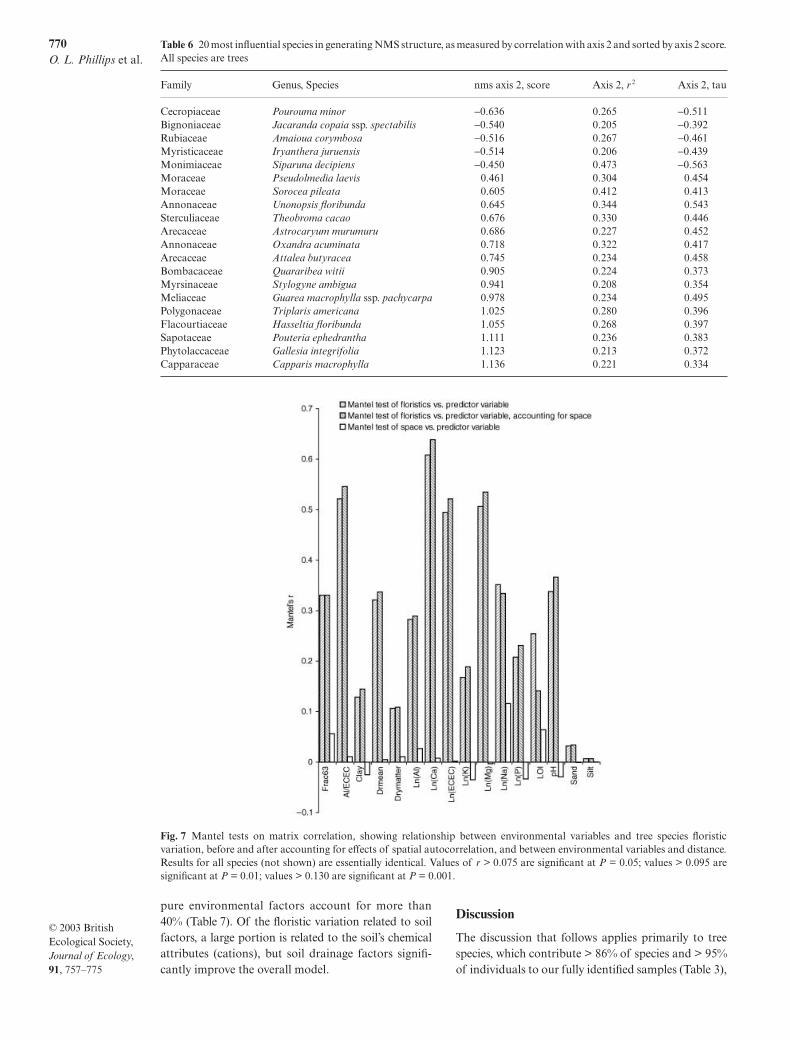
Mantel’s tests

We used the Mantel’s test on matrix correlation toexplore the relationship between environmental vari-ables and floristic variation, and conducted partialMantel tests to control for effects of spatial autocorre-lation. Variation in each environmental variable exceptfor silt and sand concentrations is significantly cor-related with floristic variation, irrespective of whetheror not the spatial pattern of intersample distance wasaccounted for (Fig. 7), and was equivalent whether theanalysis was restricted to trees or expanded to include

Fig. 5 Spatial decay in floristic similarity between sample pairs. Sørensen Index (proportion of shared species) is plotted as afunction of straight-line distance between plot centroids. Graphs show (a) floristic comparisons between all sample pairs, and (b) com-parisons separately for Pleistocene, Holocene, and Pleistocene-Holocene pairs, with 50-sample moving averages for tree species.Results for all species (not shown) are essentially identical. Floristic similarity can be described by a log-function of distance,i.e. Pleistocene pairs: S.I. = −0.0537 × ln(distance) + 0.846, R-squared = 0.334; Holocene pairs: S.I. = −0.0332 × ln(distance) +0.557, R-squared = 0.151; Pleistocene − Holocene pairs: S.I. = −0.0210 × ln(distance) + 0.440, R-squared = 0.060.

769Habitat association of Amazon trees

© 2003 British Ecological Society, Journal of Ecology, 91, 757–775

all species. The partial Mantel tests show that distancebetween samples is weakly correlated with only oneenvironmental variable (Na), consistent with our aimof sampling both geomorphic units across the wholelandscape.

Multiple regression of distance matrices

Irrespective of whether analyses are performed on theentire floristic data set or on the tree subset, distancebetween sites accounts for 10% of the variation, and

Table 5 Association of each environmental variable with NMDS axis 2 and axis 1

Variable Axis 2 R 2 Axis 2 tau Axis 1 R 2 Axis 1 tau

Drainage 0.318* −0.339 0.002 −0.040pH 0.292 0.380 0.097 0.211Al 0.241 −0.366 0.281* −0.366Ca 0.785** 0.673** 0.266* 0.378K 0.253 0.297 0.018 −0.055Mg 0.703** 0.587** 0.110 0.202Na 0.376* 0.412 0.019 0.145Al/ECEC 0.692** −0.658** 0.286* −0.375ECEC 0.433* 0.393 0.030 0.110P 0.217 0.282 0.133 0.238LOI percentage 0.056 0.140 0.003 0.094Dry matter percentage 0.080 −0.235 0.001 −0.011Clay 0.077 0.148 0.000 0.046Silt 0.060 0.145 0.001 −0.064Sand 0.350* −0.398 0.001 −0.035> 0.063 fraction 0.452* 0.443 0.014 0.079

*P < 0.05; **P < 0.01.

Fig. 6 Non-metric multidimensional sample scores (first two axes), showing relative position of sample plots in tree species space.Results for all species (not shown) are essentially identical. Curve corresponds to the division between Holocene and Pleistocenesites, except for two Holocene sites slightly below the line: BOC9 and BOC7.

770O. L. Phillips et al.

© 2003 British Ecological Society, Journal of Ecology, 91, 757–775

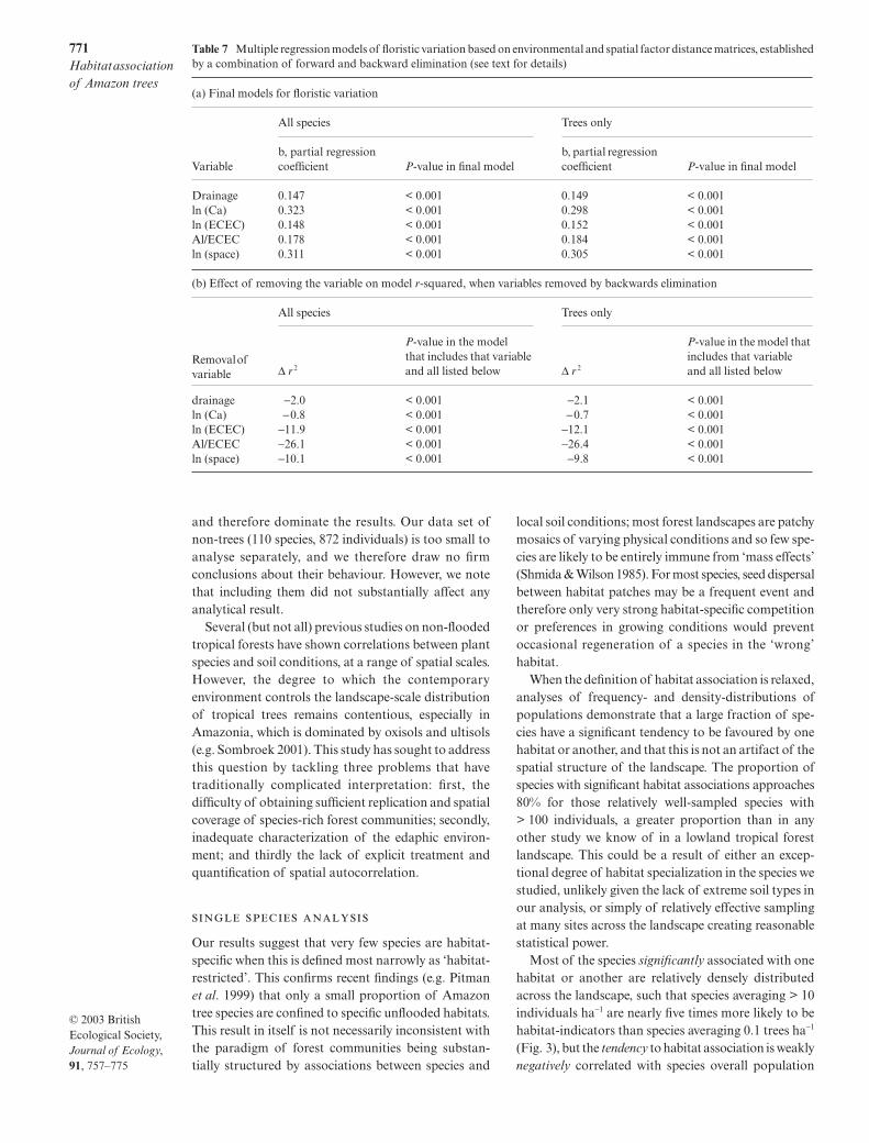
pure environmental factors account for more than40% (Table 7). Of the floristic variation related to soilfactors, a large portion is related to the soil’s chemicalattributes (cations), but soil drainage factors signifi-cantly improve the overall model.

Discussion

The discussion that follows applies primarily to treespecies, which contribute > 86% of species and > 95%of individuals to our fully identified samples (Table 3),

Table 6 20 most influential species in generating NMS structure, as measured by correlation with axis 2 and sorted by axis 2 score.All species are trees

Family Genus, Species nms axis 2, score Axis 2, r 2 Axis 2, tau

Cecropiaceae Pourouma minor −0.636 0.265 −0.511Bignoniaceae Jacaranda copaia ssp. spectabilis −0.540 0.205 −0.392Rubiaceae Amaioua corymbosa −0.516 0.267 −0.461Myristicaceae Iryanthera juruensis −0.514 0.206 −0.439Monimiaceae Siparuna decipiens −0.450 0.473 −0.563Moraceae Pseudolmedia laevis 0.461 0.304 0.454Moraceae Sorocea pileata 0.605 0.412 0.413Annonaceae Unonopsis floribunda 0.645 0.344 0.543Sterculiaceae Theobroma cacao 0.676 0.330 0.446Arecaceae Astrocaryum murumuru 0.686 0.227 0.452Annonaceae Oxandra acuminata 0.718 0.322 0.417Arecaceae Attalea butyracea 0.745 0.234 0.458Bombacaceae Quararibea witii 0.905 0.224 0.373Myrsinaceae Stylogyne ambigua 0.941 0.208 0.354Meliaceae Guarea macrophylla ssp. pachycarpa 0.978 0.234 0.495Polygonaceae Triplaris americana 1.025 0.280 0.396Flacourtiaceae Hasseltia floribunda 1.055 0.268 0.397Sapotaceae Pouteria ephedrantha 1.111 0.236 0.383Phytolaccaceae Gallesia integrifolia 1.123 0.213 0.372Capparaceae Capparis macrophylla 1.136 0.221 0.334

Fig. 7 Mantel tests on matrix correlation, showing relationship between environmental variables and tree species floristicvariation, before and after accounting for effects of spatial autocorrelation, and between environmental variables and distance.Results for all species (not shown) are essentially identical. Values of r > 0.075 are significant at P = 0.05; values > 0.095 aresignificant at P = 0.01; values > 0.130 are significant at P = 0.001.

771Habitat association of Amazon trees

© 2003 British Ecological Society, Journal of Ecology, 91, 757–775

and therefore dominate the results. Our data set ofnon-trees (110 species, 872 individuals) is too small toanalyse separately, and we therefore draw no firmconclusions about their behaviour. However, we notethat including them did not substantially affect anyanalytical result.

Several (but not all) previous studies on non-floodedtropical forests have shown correlations between plantspecies and soil conditions, at a range of spatial scales.However, the degree to which the contemporaryenvironment controls the landscape-scale distributionof tropical trees remains contentious, especially inAmazonia, which is dominated by oxisols and ultisols(e.g. Sombroek 2001). This study has sought to addressthis question by tackling three problems that havetraditionally complicated interpretation: first, thedifficulty of obtaining sufficient replication and spatialcoverage of species-rich forest communities; secondly,inadequate characterization of the edaphic environ-ment; and thirdly the lack of explicit treatment andquantification of spatial autocorrelation.

Our results suggest that very few species are habitat-specific when this is defined most narrowly as ‘habitat-restricted’. This confirms recent findings (e.g. Pitmanet al. 1999) that only a small proportion of Amazontree species are confined to specific unflooded habitats.This result in itself is not necessarily inconsistent withthe paradigm of forest communities being substan-tially structured by associations between species and

local soil conditions; most forest landscapes are patchymosaics of varying physical conditions and so few spe-cies are likely to be entirely immune from ‘mass effects’(Shmida & Wilson 1985). For most species, seed dispersalbetween habitat patches may be a frequent event andtherefore only very strong habitat-specific competitionor preferences in growing conditions would preventoccasional regeneration of a species in the ‘wrong’habitat.

When the definition of habitat association is relaxed,analyses of frequency- and density-distributions ofpopulations demonstrate that a large fraction of spe-cies have a significant tendency to be favoured by onehabitat or another, and that this is not an artifact of thespatial structure of the landscape. The proportion ofspecies with significant habitat associations approaches80% for those relatively well-sampled species with> 100 individuals, a greater proportion than in anyother study we know of in a lowland tropical forestlandscape. This could be a result of either an excep-tional degree of habitat specialization in the species westudied, unlikely given the lack of extreme soil types inour analysis, or simply of relatively effective samplingat many sites across the landscape creating reasonablestatistical power.

Most of the species significantly associated with onehabitat or another are relatively densely distributedacross the landscape, such that species averaging > 10individuals ha−1 are nearly five times more likely to behabitat-indicators than species averaging 0.1 trees ha−1

(Fig. 3), but the tendency to habitat association is weaklynegatively correlated with species overall population

Table 7 Multiple regression models of floristic variation based on environmental and spatial factor distance matrices, establishedby a combination of forward and backward elimination (see text for details)

(a) Final models for floristic variation

All species Trees only

Variableb, partial regressioncoefficient P-value in final model

b, partial regression coefficient P-value in final model

Drainage 0.147 < 0.001 0.149 < 0.001ln (Ca) 0.323 < 0.001 0.298 < 0.001ln (ECEC) 0.148 < 0.001 0.152 < 0.001Al/ECEC 0.178 < 0.001 0.184 < 0.001ln (space) 0.311 < 0.001 0.305 < 0.001

(b) Effect of removing the variable on model r-squared, when variables removed by backwards elimination

All species Trees only

Removal of variable ∆ r 2

P-value in the model that includes that variable and all listed below ∆ r 2

P-value in the model that includes that variable and all listed below

drainage −2.0 < 0.001 −2.1 < 0.001ln (Ca) −0.8 < 0.001 −0.7 < 0.001ln (ECEC) −11.9 < 0.001 −12.1 < 0.001Al/ECEC −26.1 < 0.001 −26.4 < 0.001ln (space) −10.1 < 0.001 −9.8 < 0.001

772O. L. Phillips et al.

© 2003 British Ecological Society, Journal of Ecology, 91, 757–775

densities and frequencies (Fig. 4). We draw two conclu-sions from this. First, the overall habitat associationobserved is not driven by a relatively small subset ofmore dense and frequent species, but appears to be ageneral property of many species across the landscape.Secondly, there is certainly no evidence of a decline inhabitat association for species with low populationdensities: the low proportion of low-density and low-frequency species proven to be associated with onehabitat or another reflects inadequate sampling acrossthe landscape for these species rather than a genuinebiological phenomenon.

Pitman et al. (1999, 2001) have shown that relativelyfew tree species dominate forests in west Amazonianlandscapes, suggesting that dominant species maybe relatively indifferent to environmental heterogen-eity. Our data appear to offer only weak support forthis view, as although more common species do havelower than average degrees of habitat association,there are several very common species that associatestrongly with one or other of our terra firme habitats.Examples include Phenakospermum guyanense (Rich.)Endl., Siparuna decipiens (Tul.) A. DC. and S. cristata(Poepp. & Endl.) A. DC, all of which are stronglyassociated with Pleistocene landscapes and present atdensities of > 40 individuals ha−1. However, we notethat these exceptions are understory or subcanopy spe-cies (and in the case of Phenakospermum, an over-sizedherb) that represent relatively little biomass or produc-tivity and so are hardly ‘dominants’. Thus, the regionalpattern that emerges from our data helps to reconciletwo apparently contradictory views of how Amazonforests may be put together: on the one hand that theyare largely homogeneous, even simple, communities,insensitive to edaphic changes across landscapes andconsistently dominated by an oligarchy of widely suc-cessful species; and on the other that they are complexand strongly patchy systems affected by even subtlechanges in environmental conditions.

It appears that a relatively small group of species areable to physically dominate forests almost regardless ofsoil conditions, and yet that most tree species are asso-ciated with soil factors. Our estimates of the degree ofspecies-level habitat association in our landscape maybe still too low, as statistical power to detect relation-ships is limited by insufficient sample size among the low-density species. Our data do not allow us to commentdefinitively on whether habitat-specificity is higherstill for smaller non-trees such as understory palms(Ruokolainen & Vormisto 2000), melastomataceousshrubs (Ruokolainen et al. 1997) and terrestrial pterido-phytes (Tuomisto & Poulsen 2000; Vormisto et al.2000). However, species distributions in these groupsare known to be highly non-random elsewhere in westernAmazonia (Tuomisto et al. 2003a,b).

Is it possible to reconcile our findings with a third,

non-equilibrial, view of how forests are put together(Hubbell et al. 1999; Hubbell 2001), which holds thatforests are dominated by stochastic processes such thatcomposition is substantially affected by the species thathappen to be able to disperse into and recruit in alocality? In our second set of analyses, we examinedhow landscape-scale species composition varied alongenvironmental gradients, and attempted to identify thecombined community-level effects of largely spatialprocesses such as dispersal limitation. Tree speciescomposition is affected by a general edaphic gradientfrom nutrient poor sandy-clay soils to relatively fertilesilty-clay soils (Table 5). The gradient reflects the broadPleistocene/Holocene landscape categories, but theactual variation in soil and floristic conditions (Table 6,Fig. 7) is more complex than that simple dichotomymight suggest. A substantial proportion (10%) of thevariation in forest composition is explained by the dis-tance between samples: this could be caused by ‘clas-sical’ distance decay, whereby populations are somewhatpatchy due to distance-dependent population processes(reflecting individual species’ dispersal kernels and thehistorical happenstance of where populations havebeen in the past), or an interaction with edaphic factorsthat themselves in principle could show distance decay.However, as we have shown that spatial and environ-mental factors are mostly unrelated to one another atthe landscape scale, this portion of the floristic vari-ation is likely to be attributable to distance-dependentprocesses such as dispersal limitation.

These processes do not operate equally everywhere:between pairs of Holocene samples no spatial decay incomposition is evident over a distance of > c. 10 km,suggesting efficient mixing of species, yet betweenPleistocene pairs similarity continues to decreasegently with distance across the whole study region,indicating that species may be poorly dispersed withinthis geomorphic unit. Additional multiple regressionanalyses of the whole data set using un-transformedraw distance matrices (not shown) were only able toattribute 3% of floristic variation to space, supportingthe inference that the effects of dispersal limitation areonly substantially felt over short distances. These inter-pretations are complicated by the fact that we showedthat the pattern of spatial decay in the two landscapeunits is dissimilar. There is also a possibility that someadditional, undetected, spatial effects might operate atfiner scales within habitats.

How do these results compare with other forests?Recent work by Condit et al. (2002) showed that distance-decay is much greater in a Panamanian landscape thanin two Amazonian landscapes. Our results confirm thatin parts of western Amazonia, at least, beta-diversity isless than in central Panama. However, as the Panama-nian landscape has strongly spatial climatic gradientsit was difficult to quantify the likely drivers of highbeta-diversity, which could be related to climate, geology,dispersal, or all three (Pyke et al. 2001; Duivenvoordenet al. 2002). In our data set, beta-diversity is greatest,

773Habitat association of Amazon trees

© 2003 British Ecological Society, Journal of Ecology, 91, 757–775

and the relationship between distance and compositionweakest, for Pleistocene-Holocene sample pairs, illus-trating the dominant effect of this environmental con-trast in structuring tree species composition. Multipleregression of distance matrices confirm this, showingthat a much greater proportion (40%) of landscape-scale floristic variation is explained purely by soil con-ditions than by the effects of spatial autocorrelation(10%). The chemical composition of the soil, particu-larly the concentrations of base cations and Aluminium,appears to be the most important factor, with a smallrole for drainage conditions. The soil structural vari-ables that we measured (relative contribution of clay,sand and silt) do not contribute to the best multipleregression models, suggesting that any effect theymight have on species composition is mediated by soilchemistry and drainage.

There are several reasons to suspect that the com-bined effects of substrate on landscape-scale forest flo-ristics have been underestimated in our analysis. First,although we sampled a wide range of soil variables, wemay not have captured all the substrate variation thatmay be biologically meaningful. For example: (i) oursamples were confined to the A horizon; (ii) we did notmeasure nitrogen or various biologically active traceelements; (iii) we did not quantify the mycoflora; (iv)our estimate of drainage conditions was necessarilysuperficial; and (v) we have not evaluated possible tem-poral variations in nutrient supply (cf. Newbery et al.1988). Secondly, the extent of each sample is 1.8 ha, yeta portion of environmental control is known to bemediated at a much finer spatial scale than this (e.g.Vormisto et al. 2000; Harms et al. 2001), so we did notachieve a perfect microtopographical representationof the conditions in which each plant was growing.Thirdly, our samples include all individuals as smallas 2.5 cm diameter and are dominated by juvenilesof trees. Environment-mediated effects such as com-petition may continue to operate up to much largersize-classes, possibly leading to better mapping ontosubstrates by adult populations than juvenile popula-tions (e.g. Webb & Peart 2000). Finally, our samplesare subject to substantial sampling error as we onlyinventoried a fraction of species present in each locality.

Regardless of these concerns, our results confirmthat tree species’ composition within a lowland Ama-zon landscape respond strongly to comparatively smallvariations in soil, and evidence suggests that the distri-butional patterns of most species segregate by geomor-phic unit even within a landscape with comparativelylittle soil variation. We emphasize that finding perva-sive and deterministic habitat association among Ama-zon tree species does not prove pervasive physiologicalspecialization in particular soil environments: otherbiological processes could contribute to the empiricalpatterns observed in the realized niches of these species.Indicator species of Pleistocene terraces, for example,may simply tolerate the low-nutrient, high-aluminiumconditions, rather than depend on them, and their

lower densities in the richer soil habitats may be due tothe effects of interspecific competition. Dispersal limi-tation appears to operate mostly over relatively shortdistances, confirming findings from elsewhere. Theoverall weak effect of geographical proximity at thelandscape scale suggests that these species-rich Ama-zon forest communities are structured more by in situprocesses mediated in a deterministic way by substrateconditions, than they are by spatial processes. Clearly,experimental approaches will be needed to tease apartthe biological mechanisms by which the distributionsof Amazon tree species are non-randomly controlled.

Acknowledgements

We are grateful to several colleagues for their assistanceduring the field inventories, and especially to FernandoCornejo, César Chacón, Alejandro Farfan and WilfredoRamirez. We thank Peruvian Safaris S.A., BahuajaLodge, and the people of the communities of La Torre,Palma Real, Alegría, Tres Islas, Sandoval, Jorge Chávez,Loero, Sonene, Puerto Arturo, Lago Valencia, BocaPariamanu and Sabaluyo for their generous hospitality.We acknowledge invaluable help given by FernandoCornejo in identifying some collections, and helpfuldiscussions with Tim Baker, Pippa Chapman, JonLloyd, Kalle Ruokolainen and David Wood, as well asthe contributions of three anonymous referees. MarkNewcombe helped develop Fig. 1. We thank INRENAfor providing the necessary permits for conducting thework and UNSAAC and its herbarium for support. Thiswork was funded by grant ERP-196 to the Universityof Leeds from the UK Department for InternationalDevelopment (Environment Research Department), anda UK Natural Environment Research Council ResearchFellowship to OP.

Supplementary material

The following material is available from http://www.blackwellpublishing.com/products/journals/suppmat/JEC/JEC815/JEC815sm.htm

Appendix S1 Location and geomorphology of eachforest sample in eastern Madre de Dios.

Appendix S2 Soil chemistry and structure of each for-est sample in eastern Madre de Dios.

References

Anderson, A.B. (1981) White-sand vegetation of BrazilianAmazonia. Biotropica, 13, 199–210.

Clark, D.A. & Clark, D.B. (1992) Life history diversity of canopyand emergent trees in a neotropical rain forest. EcologicalMonographs, 62, 315–344.

Clark, D.B., Clark, D.A. & Read, J.M. (1998) Edaphicvariation and the mesoscale distribution of tree speciesin a neotropical rain forest. Journal of Ecology, 86, 101–112.

774O. L. Phillips et al.

© 2003 British Ecological Society, Journal of Ecology, 91, 757–775

Clark, D.A., Clark, D.B., Sandoval, R.M. & Castro, M.V.(1995) Edaphic and human effects on landscape-scaledistributions of tropical rain forest palms. Ecology, 76,2581–2594.

Clark, D.B., Palmer, M.W. & Clark, D.A. (1999) Edaphicfactors and the landscape-scale distributions of tropicalrain forest trees. Ecology, 80, 2662–2675.

Condit, R., Ashton, P.S., Baker, P., Bunyavejchewin, S.,Gunatilleke, S., Gunatilleke, N. et al. (2000) Spatial pat-terns in the distribution of tropical tree species. Science,288, 1414–1418.

Condit, R., Ashton, P.S., Manokaran, N., LaFrankie, J.V.,Hubbell, S.P. & Foster, R.B. (1999) Dynamics of the forestcommunities at Pasoh and Barro Colorado: comparing two50-ha plots. Philosophical Transactions of the Royal Societyof London Series B. Biology Sciences, 354, 1739–1748.

Condit, R., Hubbell, S.P. & Foster, R.B. (1996) Assessing theresponse of plant functional types to climatic change intropical forests. Journal of Vegetation Science, 7, 405–416.

Condit, R., Pitman, N., Leigh, E.G. Jr, Chave, J., Terborgh, J.,Foster, R.B. et al. (2002) Beta-diversity in tropical foresttrees. Science, 295, 666–669.

Debski, I., Burslem, D.F.R.P., Palmiotto, P.A., Lafrankie,J.V., Lee, H.S. & Manokaran, N. (2002) Habitat preferencesof Aporosa in two Malaysian forests: implications for abund-ance and coexistence. Ecology, 83, 2005–18.

Denslow, J.S. (1987) Tropical rainforest gaps and tree speciesdiversity. Annual Review of Ecology and Systematics, 18,431–451.

Duellman, W.E. & Koechlin, J.E. (1991) The Reserva CuzcoAmazónico, Peru: biological investigations, conservation,and ecotourism. University of Kansas Museum of NaturalHistory Occasional Papers, 142, 1–38.

Dufrene, M. & Legendre, P. (1997) Species assemblages andindicator species: the need for a flexible asymmetricalapproach. Ecological Monographs, 67, 345–366.

Duivenvoorden, J.F. (1995) Tree species composition and rainforest-environment relationships in the middle Caquetáarea, Colombia, NW Amazonia. Vegetatio, 120, 91–113.

Duivenvoorden, J.F., Svenning, J.-C. & Wright, S.J. (2002)Beta diversity in tropical forests. Science, 295, 636–637.

Duque, A., Sánchez, M., Cavelier, J. & Duivenvoorden, J.F.(2002) Different floristic patterns of woody understoreyand canopy plants in Colombian Amazonia. Journal ofTropical Ecology, 18, 499–525.

Enquist, B.J. & Niklas, K.J. (2001) Invariant scaling relationsacross tree-dominated communities. Nature, 410, 655–660.

Faith, D.P. & Ferrier, S. (2002) Linking beta diversity, environ-mental variation, and biodiversity assessment. Science dEbatehttp://www.sciencemag.org/cgi/eletters/295/5555/636.

Fleck, D.W. & Harder, J.D. (2000) Matses Indian rainforesthabitat classification and mammalian diversity in Amazo-nian Peru. Journal of Ethnobiology, 20, 1–36.

Gentry, A.H. (1982) Patterns of neotropical plant speciesdiversity. Evolutionary Biology, 15, 1–84.

Gentry, A.H. (1988a) Changes in plant community diversityand floristic composition on environmental and geograph-ical gradients. Annals of the Missouri Botanical Garden, 75,1–34.

Gentry, A.H. (1988b) Tree species richness of upper Amazonianforests. Proceedings of the National Academy of Sciencesof the United States of America, 85, 156–159.

Grubb, P.J. (1977) The maintenance of species-richness inplant communities: the importance of the regenerationniche. Biology Reviews, 52, 107–145.

Harms, K.E., Condit, R., Hubbell, S.P. & Foster, R.B. (2001)Habitat associations of trees and shrubs in a 50-ha neotropicalforest plot. Journal of Ecology, 89, 947–959.

Hart, T.B., Hart, J.A. & Murphy, P.G. (1989) Monodominantand species-rich forests of the humid tropics: causes fortheir co-occurrence. American Naturalist, 133, 613–633.

Hubbell, S.P. (2001) The Unified Neutral Theory of Biodiversityand Biogeography. Princeton University Press, Princeton,New Jersey.

Hubbell, S.P. & Foster, R.B. (1986) Biology, chance, and historyand the structure of tropical rain forest tree communities.Community Ecology (J. Diamond & T.J. Case), pp. 314–329.Harper & Row, New York.

Hubbell, S.P., Foster, R.B., O’Brien, S.T., Harms, K.E.,Condit, R., Wechsler, B. et al. (1999) Light gap disturbances,recruitment limitation, and tree diversity in a neotropicalrainforest. Science, 283, 554–557.

Kahn, F. & Mejia, K. (1990) Palm communities in wetlandforest ecosystems of Peruvian Amazonia. Forest Ecologyand Management, 33, 169–179.

Kalliola, R., Puhakka, M., Salo, J., Tuomisto, H. &Ruokolainen, K. (1991) The dynamics, distribution andclassification of swamp vegetation in Peruvian Amazonia.Annales Botanicae Fennici, 28, 225–239.

Kalliola, R., Ruokolainen, K., Tuomisto, H., Linna, A. &Mäki, S. (1998) Mapa geoecológico de la zona de iquitos yvariación ambiental. Geoecología y Desarrollo Amazónico:Estudio Integrado en la Zona de Iquitos, Perú. AnnalesUniversitatis Turkuensis Series A II 114 (eds R. Kalliola& S. Flores Paitán), pp. 443–457. University of Turku,Finland.

Knight, D.H. (1975) A phytosociological analysis of species-rich tropical forest on Barro Colorado Island, Panama.Ecological Monographs, 45, 259–284.

Kruskal, J.B. (1964) Nonmetric multidimensional scaling: anumerical method. Psychometrika, 29, 115–129.

Legendre, P., Lapointe, F.-J. & Casgrain, P. (1994) Modelingbrain evolution from behavior: a permutational regressionapproach. Evolution, 48, 1487–1499.

Legendre, P. & Vaudor, A. (1991) The Royal-Package: Multi-dimensional Analysis, Spatial Analysis. Département deSciences Biologiques, Université de Montréal, Montreal.

Ludwig, J.A. & Reynolds, J.F. (1988) Statistical Ecology. JohnWiley and Sons, New York.

Malhi, Y., Baker, T.R., Phillips, O.L., Almeida, S., Alvarez, E.,Arroyo, L. et al. (2004) The above-ground wood producti-vity and net primary productivity of 104 neotropical forests.Global Change Biology, in press.

Malhi, Y., Phillips, O.L., Baker, T.R., Almeida, S., Frederiksen,T., Grace, J. et al. (2002) An international network to under-stand the biomass and dynamics of Amazonian forests(RAINFOR). Journal of Vegetation Science, 13, 439–450.

Mantel, N. (1967) The detection of disease clustering and ageneralized regression approach. Cancer Research, 27, 209–220.

McCune, B. & Mefford, M.J. (1999) PC-ORD. MultivariateAnalysis of Ecological Data, Version 4. MjM SoftwareDesign, Gleneden Beach, Oregon.

Newbery, D.McC., Alexander, I.J., Thomas, D.W. & Gartlan,J.S. (1988) Ectomycorrhizal rain-forest legumes and soilphosphorous on Korup National Park, Cameroon. NewPhytologist, 109, 433–450.

Newbery, D.McC. & Proctor, J. (1983) Ecological studies infour contrasting lowland rain forests in Gunung Mulunational park, Sarawak. IV. Associations between tree dis-tribution and soil factors. Journal of Ecology, 72, 475–493.

Osher, L.J. & Buol, S.W. (1998) Relationship of soil propertiesto parent material and landscape position in eastern Madrede Dios, Peru. Geoderma, 83, 143–166.

Phillips, O.L., Malhi, Y., Higuchi, N., Laurance, W.F., Nuñez,V.P., Vásquez, M.R. et al. (1998) Changes in the carbonbalance of tropical forest: evidence from long-term plots.Science, 282, 439–442.

Phillips, O.L. & Miller, J.S. (2002) Global Patterns of ForestDiversity: the Dataset of Alwyn Gentry. Monographs inSystematic Botany, Volume 89. Missouri Botanical Garden,St Louis, Missouri.

775Habitat association of Amazon trees

© 2003 British Ecological Society, Journal of Ecology, 91, 757–775

Phillips, O.L., Vásquez Martínez, R., Núñez Vargas, P.,Lorenzo Monteagudo, A., Chuspe Zans, M.-E., GalianoSánchez, W. et al. (2003) Efficient plot-based tropical forestfloristic assessment. Journal of Tropical Ecology, in press.

Pires, J.M. & Prance, G.T. (1985) The vegetation types of theBrazilian Amazon. Key Environments: Amazonia (eds G.T.Prance & T.E. Lovejoy), pp. 109–145. Pergamon, Oxford.

Pitman, N.C., Terborgh, J., Silman, M.R. & Núñez, P.V.(1999) Tree species distributions in an upper Amazonianforest. Ecology, 80, 2651–2661.

Pitman, N.C., Terborgh, J.W., Silman, M.R., Núñez, P.V.,Neill, D.A., Ceron, C.E. et al. (2001) Dominance and dis-tribution of tree species in upper Amazonian terra firmeforests. Ecology, 82, 2101–2117.

Poore, M.E.D. (1968) Studies in Malaysian rain forest. I. Theforest on Triassic sediments in Jengka forest reserve. Journalof Ecology, 56, 143–196.

Poulsen, A.D. (1996) Species richness and density of groundherbs within a plot of lowland rainforest in north-west Borneo.Journal of Tropical Ecology, 12, 177–190.

Pyke, C.R., Condit, R., Aguilar, S. & Lao, S. (2001) Floristiccomposition across a climatic gradient in a neotropical low-land forest. Journal of Vegetation Science, 12, 553–566.

Räsänen, M., Neller, R., Salo, J. & Jungner, H. (1992) Recentand ancient fluvial deposition systems in the Amazonianforeland basin, Peru. Geological Magazine, 129, 293–306.

Räsänen, M., Salo, J. & Jungner, H. (1991) Holocene floodplainlake-sediments in the Amazon – C-14 dating and paleoecolo-gical use. Quaternary Science Reviews, 10, 363–372.

Räsänen, M., Salo, J., Jungner, H. & Romero Pittman, L.(1990) Evolution of the western Amazon lowland relief:impact of Andean foreland dynamics. Terra Nova, 2, 320–332.

Rees, M., Condit, R., Crawley, M., Pacala, S. & Tilman, D.(2001) Long-term studies of vegetation dynamics. Science,293, 650–655.

Ruokolainen, K., Linna, A. & Tuomisto, H. (1997) Use ofMelastomataceae and pteridophytes for revealing phyto-geographic patterns in Amazonian rain forests. Journal ofTropical Ecology, 13, 243–256.

Ruokolainen, K. & Vormisto, J. (2000) The most widespreadAmazonian palms tend to be tall and habitat generalists.Basic and Applied Ecology, 1, 97–108.

Sabatier, D., Grimaldi, M., Prévost, M.-F., Guillaume, J.,Godron, M., Dosso, M. et al. (1997) The influence of soilcover organization on the floristic and structural hetero-geneity of a Guianan rain forest. Plant Ecology, 131, 81–108.

Salo, J. & Kalliola, R. (1990) River dynamics and natural for-est regeneration in the Peruvian Amazon. Rain ForestRegeneration and Management. Volume 6. Man in theBiosphere Series (eds A. Gómez-Pompa et al.), pp. 245–256.UNESCO and Cambridge University Press, Cambridge.

Salo, J., Kalliola, R., Hakkinen, I., Makinen, Y., Niemela, P.,Puhakka, M. et al. (1986) River dynamics and the diversityof Amazon lowland forest. Nature, 322, 254–258.

Shephard, G.N. Jr, Yu, D.W., Lizarralde, M. & Italiano, M.(2001) Rain forest habitat classification among the Matsi-genka of the Peruvian Amazon. Journal of Ethnobiology,21, 1–38.

Shephard, G.N. Jr, Yu, D.W. & Nelson, B.W. (2003) Ethno-botanical ground-truthing and forest diversity in the WesternAmazon. Advances in Economic Botany, in press.

Shmida, A. & Wilson, M.V. (1985) Biological determinants ofspecies diversity. Journal of Biogeography, 12, 1–20.

Smouse, P.E., Long, J.C. & Sokal, R.R. (1986) Multipleregression and correlation extensions of the mantel test ofmatrix correspondence. Systematic Zoology, 35, 627–632.

Sollins, P. (1998) Factors influencing species composition intropical lowland rain forest: does soil matter? Ecology, 79,23–30.

Sombroek, W. (2001) Spatial and temporal patterns of Ama-zon rainfall – consequences for the planning of agriculturaloccupation and the protection of primary forests. Ambio,30, 388–396.

ter Steege, H., Jetten, V.G., Polak, A.M. & Werger, M.J.A.(1993) Tropical rain forest types and soil factors in a water-shed area in Guyana. Journal of Vegetation Science, 4, 705–716.

ter Steege, H., Sabatier, D., Castellanos, H., Van Andel, T.,Duivenvoorden, J., De Oliveira, A.A. et al. (2000) An ana-lysis of the floristic composition and diversity of Amazonianforests including those of the Guiana Shield. Journal ofTropical Ecology, 16, 801–828.

Svenning, J.C. (1999) Microhabitat specialization in species-rich palm community in Amazonian Ecuador. Journal ofEcology, 87, 55–65.

Swaine, M.D. (1996) Rainfall and soil fertility as factorslimiting forest species distributions in Ghana. Journal ofEcology, 84, 419–428.

Terborgh, J. & Andresen, E. (1998) The composition of Ama-zonian forests: patterns at local and regional scales. Journalof Tropical Ecology, 14, 645–664.

Tuomisto, H. & Poulsen, A.D. (2000) Pteridophyte diversityand species composition in four Amazonian rain forests.Journal of Vegetation Science, 11, 383–396.

Tuomisto, H., Ruokolainen, K., Aguilar, M. & Sarmiento, A.(2003) Floristic patterns along a 43-km-long transect in anAmazonian rain forest. Journal of Ecology, 91, 743–756.

Tuomisto, H., Ruokolainen, K., Kalliola, R., Linna, A., Danjoy,W. & Rodriguez, Z. (1995) Dissecting Amazonian biodiversity.Science, 269, 63–66.

Tuomisto, H., Ruokolainen, K. & Yli-Halla, M. (2003) Dis-persal, environment, and floristic variation of westernAmazonian forests. Science, 299, 241–244.

UNESCO. (1980) Mapa de la Vegetación de America del Sur,1 : 5 000 000. Institut de la Carte Internationale du TapisVegetal, Toulouse.

Van Reeuwijk, L.P. (1995) Procedures for Soil Analysis. Tech-nical Paper 9. International Soil Reference and. Informa-tion Centre, Wageningen, The Netherlands.

Vásquez, M.R. & Phillips, O.L. (2000) Floristics and ecologyof a high-diversity forest at Allpahuayo, Amazonian Peru.Annals of the Missouri Botanical Garden, 87, 499–527.

Vormisto, J., Phillips, O.L., Ruokolainen, K., Tuomisto, H. &Vásquez, R. (2000) A comparison of fine-scale distributionpatterns of four plant groups in an Amazonian rainforest.Ecography, 23, 349–359.

Webb, C.O. & Peart, D.R. (2000) Habitat associations of treesand seedlings in a Bornean rain forest. Journal of Ecology,88, 464–478.

Wong, Y.K. & Whitmore, T.C. (1970) On the influence of soilproperties on species distribution in a Malayan lowlanddipterocarp forest. Malaysian Forester, 33, 42–54.

Received 10 September 2002 revision accepted 20 June 2003