Impacts of climate mitigation strategies in the energy sector on global land use and carbon balance K. Engström1, M. Lindeskog1, S. Olin1, J. Hassler2, and B. Smith1

1 Department of Physical Geography and Ecosystem Science, Lund University, Lund, 22362, Sweden.2Institute for International Economic Studies, Stockholm University, Sweden.

Correspondence to: Kerstin Engström (kerstin.engstrom@nateko.lu.se)

Abstract. Reducing greenhouse gas emissions to limit climate change-induced damage to the global economy and secure the

livelihoods of future generations requires ambitious mitigation strategies. The introduction of a global carbon tax on fossil

fuels is tested here as a mitigation strategy to reduce atmospheric CO2 concentrations and radiative forcing. Taxation of

fossil fuels potentially leads to changed composition of energy sources, including a larger relative contribution from

bioenergy. Further, the introduction of a mitigation strategy reduces climate change-induced damage to the global economy,

and thus can indirectly affect consumption patterns and investments in agricultural technologies and yield enhancement.

Here we assess the implications of changes in bioenergy demand as well as the indirectly caused changes in consumption

and crop yields for global and national cropland area and terrestrial biosphere carbon balance. We apply a novel integrated

assessment modelling framework, combining three previously published models (a climate-economy model, a socio-

economic land-use model and an ecosystem model). We develop reference and mitigation scenarios based on the narratives

and key-elements of the Shared Socio-economic Pathways (SSPs). Taking emissions from the land-use sector into account,

we find that the introduction of a global carbon tax on the fossil fuel sector is an effective mitigation strategy only for

scenarios with low population development and strong sustainability criteria (SSP1 “Taking the green road”). For scenarios

with high population growth, low technological development and bioenergy production the high demand for cropland causes

the terrestrial biosphere to switch from being a carbon sink to a source by the end of the 21st century.

1 Introduction

Combating climate change is one of the greatest challenges of the 21st century. Currently the world is on an emission

pathway that approaches the highest of the four Representative Concentration Pathways (RCPs; Fuss et al., 2014; Peters et

al., 2012). If emissions are not drastically curbed within the next few decades a global average surface warming of 3.7° C to

4.8° C compared to pre-industrial levels and more frequent extreme weather events will be the likely consequence (IPCC,

2014a). Such profound changes in the climate system are strongly linked with changes in the terrestrial biosphere. During the

last 250 years a share of carbon dioxide (CO2) emissions has been taken up by the terrestrial biosphere, thus referred to as a

1

5

10

15

20

25

30

carbon sink (Canadell and Schulze, 2014). The future of the terrestrial carbon sink is highly uncertain (Ahlström et al., 2012;

Ciais et al., 2013) and depends on processes and feedbacks involving the carbon cycle, nutrient dynamics, disturbances such

as wildfires, and land use, the latter driven by the demand for land to grow biomass for food, feed and fuel. Land-use and

land cover change (LULCC) are themselves drivers of climate change. During 1750-2012 deforestation and agricultural

management are estimated to have contributed 30% to anthropogenic CO2 emissions, while this share decreased to 10% in

the period 2000-2012, mainly due to decreasing deforestation rates (Canadell and Schulze, 2014; Ciais et al., 2013).

Including other greenhouse gases (GHG, e.g. methane and nitrous oxide), LULCC and agriculture were responsible for 21%

of total emissions in 2010 (Tubiello et al., 2015), the remainder stemming from the combustion of fossil fuels and industrial

processes.

Mitigation strategies are designed to slow down or limit climate change with the purpose of decreasing negative impacts on

society and the terrestrial biosphere. The transition towards carbon neutral energy sources and reduction in overall energy

use are key elements of proposed mitigation strategies. For example, in scenarios consistent with the aspiration to keep

global average temperature warming below 2°C relative to pre-industrial levels, CO2 emissions from the energy sector are

projected to be drastically decreased within the next five decades and to decline to below zero after 2070 (IPCC, 2014b). To

achieve these reductions of energy sector CO2 emissions from the energy sector, one proposed mitigation measure is to

introduce a global carbon tax which creates incentives to reduce overall energy use and to replace fossil fuels with renewable

energiessources, including bioenergy. Bioenergy can be derived from energy crops or residues from other land uses such as

forestry (Haberl et al., 2010). An inevitable effect of increased bioenergy use will be an increasing demand for land (Wise et

al., 2009; Hassler and Sinn, 2016b), the displacement of lands formerly used for traditional agriculture, or the extension of

land use into areas occupied by natural ecosystems. IMoreover, not all bioenergy systems lead to net emissions reductions,

especially if the carbon debt implied by (carbon released when land was cleared initially for bioenergy production) is

included (Fargione et al., 2008),. not all bioenergy systems lead to net emissions reductions.

The demand for food and feed is dependent on societal and technological development, e.g. population growth, changes in

diets and yield management. Socio-economic scenarios describe the joint evolution of different aspects of development.

Here we apply a novel Integrated Assessment Modelling (IAM) framework based on existing, established component models

of ecosystem carbon cycling and crop yields, land use and energy sector responses to climate and economic development to

explore the impacts of a global carbon tax on fossil fuels on global land use and land-atmosphere carbon exchange of the

imposition of a global carbon tax on fossil fuels as a mitigation measure. Our approach is offered as an alternative – parsimonious – method, compared with the IAM-generated public SSP (Shared Socio-economic Pathways;

O’Neill et al., 2017) projections (Riahi et al., 2017; SSP database, 2015), for interpreting the SSP scenarios and relating them to climate, emissions, ecosystem impact, land use and energy sector development in a coherent way. The scenarios are not predictions, but aim at providing an independent set of consistent SSP realisations based on the SSP narratives and harmonized key input data, such

2

5

10

15

20

25

30

as population and economic growth. They serve to investigate and highlight interactions between societal and biophysical processes that might be important, e.g. leading to non-obvious outcomes. Specifically, we aim at quantifying the effects of a global carbon tax on fossil fuels for eachgiven the assumptions implied

by each SSP regardingon food consumption, yield development and cropland, and of the combination of these driving forces

on the terrestrial carbon balance.

2 Methods

2.1 Reference and mitigation scenarios in the IAM framework

We developed two sets of scenarios based on the socio-economic key-elements of the SSP narratives (O’Neill et al., 2017),

such as population and technology (Fig. 1). The SSP narratives outline five plausible pathways that global societal

development could follow in the 21st century and are characterized by key elements, such as population, equity, economy,

trade, lifestyle, policies, technology and energy intensity (O’Neill et al., 2017). The SSP narratives do not take into account

Ppotential impacts of climate change or new climate policies are not included, and the SSP narratives can thus be considered

reference scenarios with respect to climate change (O’Neill et al., 2013). The first set of scenarios used in this study is

elaborated by translating the key elements of the SSP narratives into model parameter values. As no new climate polices

were considered, the scenarios of this first set are hereinafter referred to as reference scenarios. A second set of scenarios

(“mitigation scenarios”) was elaborated, considering a mitigation strategy consistent with relevant aspects of the SSP

narratives. Model parameter values were selected reflecting the assumed mitigation strategy in the respective scenario.

Mitigation measures considered were limited to consequences of the introduction of a global carbon tax on fossil fuels

targeting overall reductions in energy use and the replacement of fossil fuels with renewable energies, including bioenergy.

Carbon taxes are generally regarded as an effective economic incentive to reduce greenhouse gas emissions and lead to less

volatility in emissions prices than quantity restrictions as in carbon trading schemes (Golosov et al., 2014; Hassler et al.,

2016a). Instead, the tax can be set equal to the expected damage of a marginal unit of emissions allowing market participants

to take these damages into account when making economic decisions.

3

5

10

15

20

Figure 1. The SSP scenarios of global socio-economic development in the 21st century in their space of challenges for mitigation and adaption (adapted from O’Neill et al. 2013) and selected key elements: growth of population, growth of the economy, lifestyle, policy orientation and technological development (O’Neill et al., 2017).

Mitigation through carbon sequestration, e.g. by afforestation schemes or carbon capture and storage technology, was not

considered. However, the five mitigation scenarios encompass strategies that are assumed to affect the speed and strength of

technological growth of energy production technologies and infrastructure, alongside the level of global carbon tax imposed

in the mitigation scenarios. Instead of defining a target (e.g. global average temperature increase of less than 2°C) and

designing a climate policy that is likely to achieve this target (as in the Shared Policy Assumptions, SPAs;, see Kriegler et

al., 2014), we chose to assign mitigation strategies that are consistent with the challenges for mitigation implied by each SSP

narrative. For example, the level of the global carbon tax is optimal in scenarios with low challenges to mitigation with while

with larger challenges to mitigation itthe carbon tax level would be less than optimal, while the level of the global carbon tax

is optimal in scenarios with low challenges to mitigation. The key characteristics of the SSP narratives (Fig. 1) result in

varying challenges for mitigation , as for example the high energy demand in SSP5 “Taking the highway” and the slow

technological change in SSP3 “A rocky road” (O’Neill et al., 2017). The differences in non-climate policies and institutions

likewise contribute as well to varying challenges for mitigation. For example, the environmental awareness and effective

institutions in SSP1 “Taking the green road” decrease the challenges for mitigation compared to e.g. SSP5 “Taking the

highway” (O’Neill et al., 2017). Thus, high challenges for mitigation are not the result of political resistance per se in the

SSP narratives. The presented novel IAM framework (Fig. 2) combines three previously published models, which are

described in more detail in Ssection 2.2.

4

5

10

15

20

Figure 2. Overview of the novel Integrated Assessment Modelling (IAM) framework showing input data sets in blue, component models in orange and information flows/intermediate results in green. Final results are displayed in red. The Representative Concentration Pathways (RCPs) are input to the climate model and the Shared Socio-economic Pathways (SSPs) are input to the climate-economy model and the land-use model. Damage to gross world product (GWP) is input to the land-use model. signifies the distances between emissions predicted by the climate-economy model and implied by RCPs, used as inverse weights the to create yield time series as input to the land use model.

First, the climate-economy model calculates the social cost of carbon emissions from the energy sector, equivalent with the

optimal carbon tax and the damage to gross world product (GWP). Damages are determined as a function of simulated mean

global temperature in turn driven by the endogenously determined emission path. Thus, the climate-economy model is used

to create emission scenarios, assess estimate damage to GWP and simulate renewable and fossil energy demands (for details

see Sectionsection. 2.2.1). Further, the SSPs provide input data for population and economic development and characterize

technological change and consumption patterns, required as input to a socio-economic land-use model. The land-use model

reconciles demand for food, feed and bioenergy implied by the scenario assumptions with the biophysically-determined

supply (productivity) of these commodities per unit land area on a country-by-country basis, and translates this into cropland

changes (for details see Sectionsection. 2.2.2). The land-use model uses yield scenarios, which are the result of calculating

the distances of the emission scenarios (indicated by ∆ in Fig. 1) to the RCPs and using these as inverse weights to create

yield time series (Appendix A5; Engström et al., 2016a) based on simulated cropland productivity from an ecosystem model

(for details see Sectionsection. 2.2.3). Using the inverse weights on the RCP driven cropland productivity ensures the

consistency of inputs to the land-use model, i.e., the bioenergy demand and the yield time series implied (as both are driven

by the same emissions pathway).

5

5

10

15

20

The land-use model uses the scenario-specific damage to GWP (downscaled to damage on gross domestic product (GDP),

see Ssection 2.2.2) and yield data to explore the indirect impact of damages of GDP on food consumption (less income, less

consumption) and yield development (less income, less investments in yield improving technologies), as well as the direct

impact of bioenergy demand on cropland area in each country. Resulting cropland changes are downscaled to grid cell level

(see Appendix A7) and enabling the impact on terrestrial carbon balance of cropland changes –, taking into account the

mitigation-derived amelioration of climate change –, to beis estimated by the ecosystem model.

2.2 Component models

2.2.1 Climate-economy model

The climate-economy model is a modern macro model with micro-foundations to represent the economy.1, suited to studying

howThis model allows us to study how, for example, different carbon taxes affect the economy by allowing taxes to be an

input in the profit maximization of energy providing firms. The model is also in line with macroeconomics as taught to

graduate students of economics. The climate-economy model It is a dynamic general-equilibrium model that predicts the

joint evolution of the global climate and economy, operating at the global scale (Golosov et al., 2014). FIn the model,

forward-looking agents decide how much to consume and save. Profit maximizing firms operating within goods and energy

markets make production decisions (regulating supply and demand), taking prices and taxes as given. The use of three

different types of energy, namely oil, coal and clean energy (renewables and nuclear, free of fossil carbon emissions), is

determined as a market outcome such that supply equals demand at all points in time. The fact that markets are modelled

explicitly makes the model different from the most popular economic models employed in used to study climate change

studies, and therefore well suited to study how policies, for example carbon taxes at different levels, affect the market

outcome.

Golosov et al. (2014) show that the convex damage function constructed by Nordhaus (2008) using a bottom-up approach in

combination with a logarithmic relation between atmospheric CO2-concentration and forcing implies that the logarithm of

GWP is approximately linear in the CO2-concentration. Thus, a marginal unit of airborne carbon has an approximately

constant percentage impact on GWP independent of the CO2 concentration. Golosov et al. (2014) calculate the damage

elasticity (γ) to a factor of 2.38 × 105 per airborne GtC implying that an extra GtC in the atmosphere reduces the flow of

GWP by 2.38 × 103 percent. Due to the large uncertainty about this value, our scenarios will also include substantially

higher damage elasticities. Finally, Golosov et al. (2014) show that the optimal carbon tax is proportional to GWP with a

proportionality factor given by the product of the expected value of γ and the carbon duration D defined as in Eq. (1):

1 Supply and demand are derived from an explicit description of the objectives and constraints of forward-looking

market participants operating in a potentially stochastic environment.

6

5

10

15

20

25

D ≡∫0

∞

e−ρt ψ ( t )dt (1)

where ρ is the rate at which future welfare is discounted and ψ (t ) is the share of a unit of carbon emissions that remain

airborne t units of time after it was emitted.

The model endogenously solves for the use of the three types of energy and carbon emissions. Key parameters determining

the emissions paths are the rate of growth in the efficiency of producing coal (A2,g) and clean energy (A3,g, where clean energy

includes nuclear energy and renewables) and the elasticity of substitution (se) between these types of energy in the

production of final goods. These efficiencies measure the amount of energy services produced per unit of labour input (man

hours) in the different respective energy sectors. Over time, technological improvements increase the energy efficiencies. A

higher growth rate in the efficiency of production of coal or clean energy (clean energy) production leads, as long as other

variables are held constant, to slower price growth and faster growing use of the respective energy typecoal (clean energy).

The sensitivity of this mechanism is determined by how substitutable the different types of energy are in the production of

final goods, parameterized by the elasticity of substitution (se). Baseline assumptions about these parameters are listed in

Table 1 and are assumed to be amenable for scenario specific developments.

To characterise the socio-economic developments in the reference and mitigation scenarios we make assumptions about the

parameters as shown in Table 1. The technological growth rates are mainly influenced by the technological development

described in the SSP’s, but to a lesser extent also by the mitigation scenario assumption of s (stronger technological growth).

Strictly speaking, the economic model does not contain a mechanism whereby policy makers could affect these growth rates.

However, it would be straightforward to allow the growth rates to be determined by how R&D efforts are allocated between

different uses. This would make it possible for policy makers to partly control relative and absolute technology growth rates

without important changes in the model’s predictions (see e.g., Hassler et al., under review 2016b, for an example of

endogenous energy-related technical change). A similar argument can be made regarding the substitution elasticity where it

is assumed that policy makers can facilitate a transition to a cleaner energy production by slightly increasing the elasticity.

However, in all cases, the elasticity is fairly close to unity.

Table 1. Parameters in climate-economy model modified for scenarios.

Parameter Abb

reviation

Baseli

ne value

Unit

Growth in production

efficiency of coal

A2,g 2 annual growth in %

7

5

10

15

20

25

Growth in the efficiency of

clean energy technologies

A3,g 2 annual growth in %

Substitutions elasticity

between different energy sources

se 0.95

Damage elasticity factor γ 2.38 10-5 per airborne

GtC

Level of carbon tax τ 0, 1 fraction of optimal

carbon tax

2.2.2 Land-use model and coupling to the climate-economy model

The land-use model PLUM (Parsimonious Land-Use Model) simulates changes in cropland coverage on the basis of changes

in cereal, meat and milk consumption and changes in cereal yield in 168 countries (Engström et al., 2016b). Calculations of

food demand are dependent on population and economic development and are described by statistical relationships revealed

by historical country-level statistics from reported data (FAOSTAT, 2016). The coefficients characterizing these

relationships are used as scenario parameters. Values for scenario parameters are based on the SSP characteristics as

previously described in Engström et al. (2016a). Population, economic development and the share of urban population on

total population are input to PLUM and are used as provided by the SSP database (SSP-Database, 2015). Changes in

expected production are simulated via a global rule-based trade mechanism. The expected cereal production together with

cereal yield is used to simulate changes in cereal land. During the simulation period it is assumed that actual national yields

in PLUM are changing towards potential yield, simulated for multiple RCP × GCM climate trajectories by the ecosystem

model LPJ-GUESS (see Sectionsection. 2.2.3 and Engström et al., 2016a), depending further on each scenario’s

technological growth, economic development and technology transfer rate. Finally, changes in total cropland are assumed to

be proportional to changes in cereal land, using the actual proportions of cereal land to total cropland in 2000 (Engström et

al., 2016b). In previous applications of PLUM (Engström et al., 2016a) the static feed ratio (assumption as to how much of

the consumed meat is produced from cereal feeds vs. grazing) was identified as a cause for underestimation of cropland

demand for scenarios with meat-rich diets. Here we assumed the feed ratio to increase proportional to increases in

consumption of animal products if the initial feed ratio is very low, restricted by a scenario specific maximum for the feed

ratio (feedRatioCap; see Appendix A1).

The simulated damage to GWP from the climate-economy model was downscaled to country level GDP, adjusting the shares

covered by high, medium and low income countries, depending on the level of social equity of each SSP (equity, see

Appendix A2). This formulation reflects the assumption that low income and vulnerable countries would not receive much

8

5

10

15

20

support by high income countries to deal with the consequences of climate change in the case of low equity. The

downscaling approach reinforces the pattern of decreasing economic inequalities across low, medium and high income

countries for high equity scenarios, while it slowings down the decrease ining income gap for scenarios with low equity (see

Table A. 1, Appendix A2).

The output of clean energy from the climate-economy model was used to derive bioenergy scenarios, which were then

translated into explicit cropland demands for bioenergy in PLUM. To arrive at the bioenergy scenarios we assumed that the

shares of different clean energy sources (nuclear and renewables, i.e. hydro, wind, solar and bioenergy) projected by the

World Energy Outlook (WEO) scenarios (current policy, new policy and 450ppm; Appendix A3; OECD/IEA, 2012) are

representative for scenarios with high, medium and low challenges towards mitigation in the SSP challenge space (Fig. 1).

The resulting projections of bioenergy are assumed to be produced from a range of available sources, such as industrial

waste, forestry residues, agricultural by-products and energy crops. Energy crops in the WEO scenarios are defined as

“those (crops) grown specifically for energy purposes, including sugar and starch feedstocks for ethanol (corn, sugarcane and

sugar beet), vegetable-oil feedstocks for biodiesel (rapeseed, soybean and oil palm fruit) and lignocellulosic material

(switchgrass, poplar and miscanthus)” (OECD/IEA, 2012). In PLUM we only explicitly model the share of bioenergy

produced from energy crops (excluding lignocellulosic feedstocks), which was 3% in 2000 (OECD/IEA, 2012). The future

contribution of energy crops to total bioenergy potential is highly uncertain depending on assumptions as to available

croplands and yield development, but considering sustainability constraints has been suggested to fall within the range of

from 30-50% in 2050 (Haberl et al., 2010). Lignocellulosic feedstocks are expected to play a major role in future bioenergy

production, but as they are excluded here we assume a lower contribution of energy crops to total bioenergy of maximum at

most 15% in 2100 (shareBEcr, see Appendix A4). The modelled bioenergy production occurs here predominantly on

cropland that was set aside in previous time-steps due yield improvements and/or decreasing demand, but if this is not

availableonce such areas are used up it is expanded into remaining natural vegetation (grasslands and or forest; see Appendix

A4). Bioenergy production is assumed to be predominantly produced in countries with large bioenergy production today as

well as countries with sufficient remaining natural vegetation (in cases where bioenergy cannot be produced on abandoned

cropland). Furthermore, bioenergy production efficiency is assumed to increase at different rates depending in the scenario,

bound by the upper range of values reported today (efficiencyBE see Appendix 4; Börjesson and Tufvesson, 2011).

2.2.3 Ecosystem model, downscaling cropland and the terrestrial carbon balance

The managed land version of the dynamic vegetation-ecosystem model LPJ-GUESS (Smith et al. 2001, 2014; Lindeskog et

al., 2013), was used to simulate cereal yields (wheat, maize, millet and rice) as input to PLUM as in Engström et al. (2016a).

The simulations capture the impact of climate change on yield developments on a 0.5 × 0.5° global grid through changes in

precipitation, temperature patterns and CO2 concentration (derived from the RCPs, see Engström et al., 2016a), through

direct biophysical effect and also by adaoptation ofting the sowing timealgorithm to changes in climate. No other changes

(e.g., the introduction of new varieties) in cropland management were considered in these simulations for the present study.

9

5

10

15

20

25

30

Simulated yields from LPJ-GUESS were used to construct per grid cell anomalies, which were then applied on a grid cell

basis toon actual and potential yields taken Mueller et al. (2012) for the year 2000. For use in PLUM, actual and potential

yields were aggregated from grid cells to country level using crop area fractions from the MIRCA2000 data set (Portmann et

al., 2010), which was used to calculate the initial yield gap. The SSP-RCP matrices for the reference and mitigation

scenarios (Appendix A5) were used to weight the simulated climate driven yield anomalies for the four RCPs together.

During the simulations, the yield gap does not change as a proportion of potential yield (see Engström et al. (2016a) for

details on how the yield gap is modelled). However, as potential yield is computed dynamically based on climate input,

resulting in an anomaly relative to baseline conditions, the absolute magnitude of the yield gap can change.

The country-level changes in cropland area simulated with PLUM were applied to a base map of current land cover

(cropland and grassland) extent on a 0.5 × 0.5° global grid (Hurtt et al. 2011). A downscaling algorithm was used to

disaggregate land cover from country to grid cell level based on a weighted combination of proximity to existing cropland

and suitability based on simulated potential crop productivity, capturing both expansion and contraction of current land

cover extent. A detailed description of the downscaling algorithm is provided in Appendix A7.

To estimate the combined effects of biophysical drivers and land use change on biospheric terrestrial carbon balance, we

applied LPJ-GUESS globally on the 0.5 × 0.5° grid of the downscaled land use data, simulating natural vegetation (also

encompassing forest), cropland and pasture and the dynamic transitions between these land cover types (Lindeskog et al.,

2013). Natural vegetation in the model emerges as the result of growth and competition for light and soil resources among

woody plant individuals and a herbaceous understorey in each of a number (5 in this study) of replicate patches (0.1 ha),

representing stochastic variation in stand age following disturbance across the landscape of a simulated grid cell (Smith et

al., 2014). Multiple plant functional types (PFTs) co-occur and compete within each patch, and age/size classes are

distinguished for trees, capturing effects of stand demography on biomass accumulation and turnover. Nitrogen cycle effects

on ecosystem carbon balanceC-N interactions were taken into account, following Smith et al. (2014). Pasture is represented

by herbaceous (C3 or C4 grass) PFTs, harvested yearly. For the carbon balance simulations, cCropland wasis represented by

wheat as a proxy for all C3 crops and maize as a proxy for all C4 crops – including energy crops – following the

implementation of Olin et al. (2015), with relative areas aggregated from the MIRCA2000 data for the year 2000 (Portmann

et al., 2010), and taken to represent all C3 (wheat) and C4 (maize) crops globally, including energy crops. Irrigation was

applied for cropland, according to historical global irrigation data for the year 2000 (Portmann et al., 2010), while nitrogen

fertiliszation followed historical data for the period 1901-2006 (Zaehle et al., 2010). Tillage and the planting of cover-crops

were considered in all simulations (Olin et al., 2015), and no future changes in management for a given cropland type were

considered.

For the historical period (1700-2000), model input encompassed cropland, pasture and natural area fractions for 1700-2000

from Hurtt et al. (2011), global atmospheric CO2 concentrations for 1850-2000 from the CMIP5 archives (Taylor et al.,

2012) and nitrogen deposition data for 1850-2000 from Lamarque et al. (2011). For future simulations (2001-2100) climate

input to the ecosystem model simulations was provided by bias-corrected fields of mean monthly temperature, precipitation

10

5

10

15

20

25

30

and incoming shortwave radiation for the atmosphere-ocean general circulation model (GCM) IPSL-CM5A-MR (IPSL,

Dufresne et al., 2013). IPSL was selected as it simulates changes in carbon balance in response to the simulated LULCC and

climate change that are located in the middle of the ensemble spanned by all GCMs (Ahlström et al., 2012), which was

confirmed by running three additional GCMs (GFDL-CM3 (Donner et al., 2011), MIROC5 (Watanabe et al., 2010) and

MRI-CGCM3 (Yukimoto et al., 2012)) for a scenario (SSP2m) with medium LULCC that is located in in the middle of the

range spanned by all scenarios (SPS1-5,2r,m) and RCP4.5. GCM-generated forcing fields were bias corrected relative to

observed historical climate from the CRU TS3.0 dataset (Mitchell and Jones, 2005) and downscaled to the grid of the land

use data, following Ahlström et al (2012). Carbon pools in the model were initialized to equilibrium with the early-20th

century historical climate by means of a 500 year “spin-up” forced by prescribed 1700 land cover, 1850 atmospheric CO2

concentration and nitrogen deposition, 1901 nitrogen fertilizer applications for cropland, and detrended monthly climate time

series for 1850-1879, cycled repeatedly.

Carbon cycle simulations were performed for the scenario period 2001-2100, separately for the reference and mitigation

scenarios for each SSP. Time-varying cropland-area fractions simulated by PLUM were applied as anomalies relative to

baseline (2000) land use from the Hurtt et al. (2011) product, downscaled from country to grid cell level, as described above.

Separate simulations were performed for each RCP × GCM combination; nitrogen deposition data were taken from

Lamarque et al. (2011) for the relevant RCP. Relative crop type distribution, irrigation, nitrogen application (after 2006) and

tillage intensity were kept constant at modern (2006) levels. Model outputs were aggregated to grid cell averages for each

SSP, weighting simulations according to the probabilistic mapping of each SSP to each RCP shown in the Appendix (Table

A.3).

2.4 Parameterizing the models for the reference and mitigation scenarios

2.4.1 Parameter settings for the climate-economy model

The scenarios for energy, atmospheric carbon dioxide concentration and damage on GWP for the reference and mitigation

SSPs were created by parameterising the climate-economy model accordingly to the development described in the SSP key

elements (O’Neill et al., 2017), listed in Table 2. Additionally to these key elements we included the second axis of the

challenge space, the challenges for adaptation, to derive a sensitiveguide the parameterization of theimpose a damage

elasticity factor (γ) for each scenario. In the climate-economy model, the damage factor γ describes the impact of emissions

and climate change on GWP. Higher γ means that in mitigation scenarios emissions will need to be decreased substantially to

avoid anticipated higher damages.

Table 2: Challenges for mitigation and adaptation and energy-related key elements for the five SSPs.

Key element SSP1: Taking the SSP2: The middle SSP3: A rocky SSP4: A road SSP5: Taking the

11

5

10

15

20

25

30

green road of the road road divided highway

Challenge for

adaptation

low medium high high low

Challenge for

mitigation

low medium high low high

Energy

technological

change

Directed away

from fossil fuels,

toward efficiency

and renewables

Some investment in

renewables but

continued reliance

on fossil fuels

Slow technological

change, directed

toward domestic

energy sources

Diversified

investments

including

efficiency and low-

carbon sources

Directed toward

fossil fuels;

alternative sources

not actively

pursued

Carbon

intensity

low medium high in regions

with large domestic

fossil fuel

resources

low/medium high

Energy

intensity

Low Uneven, higher in

LICs

High Low/medium High

Fossil

constraints

Preferences shift

away from fossil

fuels

No reluctance to

use unconventional

resources

Unconventional

resources for

domestic supply

Anticipation of

constraints drives

up prices with high

volatility

None

The challenges for adaptation are low for SSP1 “Taking the green road” and SSP5 “Taking the highway”, medium for SSP2

“Middle of the road” and high for SSP3 “A rocky road” and SSP4 “A road divided”, which was translated into quantitative

values for the damage factor γ, see Table 3. Golosov et al. (2014) show that γ of 5× 105 per airborne GtC fairly well

approximates a middle-range climate sensitivity of 3°C (i.e. a doubling of the atmospheric carbon pool leads to a 3°C

increase in global mean temperature) and a damage function following Nordhaus (2007). Acknowledging the limited

evidence for the calibration of γ, we choose this to represent a relatively benign situation and also use higher gammas. For

the scenarios we therefore chose 5, 10 and 15 × 105 per airborne GtC  to represent low, medium and high damage factors,

encompassing reasonable uncertainty in this factor across SSPs. 

The parameter settings for γ are assumed to be equal in the reference and mitigation scenarios per SSP. For the reference

scenarios no carbon tax is assumed (τ=0), see Table 3.We chose Nordhaus discount rate for all scenarios (1.5% per year).

12

5

10

As for the reference scenarios, the SSP narratives form the basis of the mitigation scenarios. In addition to introducing

carbon taxes, mitigation strategies could, as described above, encompass the following changes relative to the reference

scenario: (1) reduced growth of extraction efficiency of coal; (2) increased growth of efficiency of green technologies; and

(3) The increased substitution elasticity in order to further stimulate the production of green (=clean) energy.

All these changes should be Parameter choices consistent with the storylines of the SSPs and with the challenges for

mitigation (high, medium, low) of the respective SSP. Parameter choices are shown in Table 3. The level of the carbon tax τ

(Table 1) for the mitigation scenarios is specified as a fraction of the optimal carbon tax (τ). We assumed that the mitigation

strategies for scenarios with low challenges to mitigation (SSP1 “Taking the green road” and SSP4 “A road divided”) imply

an optimal carbon tax (τ =1). The optimal carbon tax reduces emissions to the level where the costs of avoiding emissions

and the cost of avoided damages are at equilibrium. The mitigation strategy for SSP2 “Middle of the road” (medium

challenge to mitigation) consists of 30% of the optimal carbon tax (τ =0.3). For scenarios with high mitigation challenges

(SSP5 “Taking the highway” and SSP3 “A rocky road”) we assumed that the mitigation strategy is 10% of optimal carbon

tax (τ =0.1). This reflects the belief contention that political problems associated with introducing a global tax may lead to a

tax substantially lower than the optimal (see Appendix A6).

13

5

10

Table 3. Parameter settings in the climate-economy model (see Table 1) for reference (r) and mitigation (m) scenarios based on the SSPs and the challenge for adaptation (damage elasticity factor, γ) and mitigation (carbon tax, τ, as a proportion of optimum, for mitigation scenarios).

ScenarioA2,g A3,g se γ τ

r m r m r m r m r m

SSP1 “Taking the green road” 0.5 0.0 2.5 2.5 0.80 0.95 5 5 0.0 1.0

SSP2 “The middle of the road” 2.0 2.0 1.5 2.0 0.85 1.05 10 10 0.0 0.3

SSP3 “A rocky road” 1.2 1.2 1.0 1.2 0.95 0.95 15 15 0.0 0.1

SSP4 “A road divided” 1.5 1.0 1.5 2.0 0.90 1.05 15 15 0.0 1.0

SSP5 “Taking the highway” 2.2 2.0 0.0 0. 0 1.05 1.20 5 5 0.0 0.1

2.4.2 Parameter settings for land use model

TFor the parameterization of the land use model PLUM we relied on the parameterization as infollowed Engström et al.,

(2016a). For example, parameters steering the yield gap (development, investment and distribution of technologies

improving yields) were set according to the SSP narratives and the relevant SSP key elements. For SSP1 “Taking the green

road” it was assumed that the “increasingly effective and persistent cooperation and collaboration of local, national and

international organizations and institutions” (O’Neill et al., 2017) would result in a strong trend of technological transfer and

thus globally decreasing yield gaps (and thus increasing crop yields). The scenario parameters newly introduced in this

study, for example, the maximum feed ratio feedRatioCap (Table 4, Appendix A1), were parameterised as listed in Table 4.

The second new scenario parameter is equity which directly relates to the human development key element “Equity” of the

SSPs as described in O’Neill et al. (2017). Equity is described to be high for SSP1 “Taking the green road” and SSP5

“Taking the highway”; medium for SSP2 “Middle of the road” and SSP4 “A road divided”; and low for SSP3 “A rocky

road” (O’Neill et al., 2017). In PLUM, equity steers which downscaling approach for damage to GWP is used, see Table 4.

The implementation of bioenergy in PLUM introduced two additional scenario parameters: shareBEcr, which describes the

increase of bioenergy produced from energy crops, and efficiencyBE, which accounts for efficiency improvements in energy

conversion. These two scenario parameters were permitted to vary across the SSPs, and for the reference and mitigation

cases. The share of bioenergy that was produced from energy crops in the period 2000-2010 was 3% and was assumed to

increase to up to 6% in 2100 for the reference scenarios with sustainability focus (SSP1 “Taking the green road”) and

reference scenarios which, at least partly, are strongly reliant on local energy sources (SSP3 “A rocky road” and SSP4 “A

road divided”). For the fossil fuel focused SSP5 “Taking the highway” no changes from the initial values for the bioenergy

14

5

10

15

20

scenario parameters were made, neither for reference or mitigation scenariocases. For the mitigation version case of SSP1

“Taking the green road” the share of bioenergy crops was assumed not to increase further than in the reference scenariocase,

due to the fact that the use of cropland for bioenergy production and its effect on sustainability can be negative in some

cases.

15

Table 4. Parameter settings in the PLUM land use model for feedRatioCap (0.1-0.3: feed ratio increases for countries with feed ratios below 0.1-0.3 up to 0.1-0.3, that is a maximum 10%-30% of meat is produced with cereal feed for countries with initially low feedRatios), equity (1=high equity distribution, 0=equal distribution, -1=low equity distribution), the share of bioenergy that is produced from bioenergy crops in 2100 (shareBEcr, %, 3% being the initial value in 2100), the conversion efficiency of energy in biomass to bioenergy that is achieved in 2100 (efficiencyBE, %, 65% being the initial value in 2000) for reference (r) and mitigation (m) scenarios based on the SSPs.

By contrast, for SSP4 “A road divided”, which, as SSP1 “Taking the green road”, has a low challenge to mitigation but less

focus on sustainability, it was assumed that bioenergy production from energy crops would increase, reaching to up to 9% in

2100. SSP3 with its high challenge to mitigation was assumed to keep the share of bioenergy crops as in the reference

scenariocase, but increase the efficiency in bioenergy conversion slightly.

3 Results

3.1 Global energy scenarios, atmospheric carbon, damage to GWP and cropland development

With no mitigation, global energy use increases steeply for all scenarios, least for SSP1 “Taking the green road”, and spans a

range of 1000-2000 EJ by 2100 (Fig. 3). The predominant energy sources across the reference scenarios differ. While in

SSP5 “Taking the highway”, fossil fuel dominates, in all other reference scenarios, renewable energies and bioenergy

contribute to the rising energy demand, especially for the sustainability-oriented SSP1 “Taking the green road”. The

introduction of a global carbon tax on fossil fuels as a mitigation strategy effectively reduces the energy consumption to

around 1000 EJ in 2100 for all scenarios (Fig. 3). However, the contributions of fossil fuels, renewable energies and

bioenergy to total energy supply differ greatly across the mitigation scenarios and reflect the varying associated levels of

global carbon taxes.

16

ScenariofeedRatioCap equity shareBEcr efficiencyBE

r m r m r m r m

SSP1 “Taking the green road” 0.1 0.1 1 1 6 6 68 70

SSP2 “The middle of the road” 0.2 0.2 0 0 3 6 66 68

SSP3 “A rocky road” 0.1 0.1 -1 -1 6 6 65 66

SSP4 “A road divided” 0.2 0.2 0 0 6 9 66 68

SSP5 “Taking the highway” 0.3 0.3 1 1 3 3 65 65

5

10

15

20

25

30

Figure 3. Primary energy demand (0-2000 EJ; vertical axis of internal panels) simulated by the climate-economy model for the reference (r) and mitigation (m) versions of each SSP scenario (see Fig. 1) for the time period 2010-2100 (horizontal axis of internal panels). The dashed lines indicate the total primary energy of the official SSP realisations (SSP database, 2015). The reference scenarios are compared with the baseline marker scenarios and the mitigation scenarios are compared with the marker SSP1-RCP2.6, SPP2-RCP4.5, SSP3-RCP4.5, SSP4-RCP2.6 and SSP5-RCP6.0 scenario respectively.

Effective, globally collaborating institutions and environmental awareness contribute to low challenges for mitigation in SPP

1 “Taking the green road” and result in high carbon taxes (115 US$ per ton carbon at 2010 GWP), decreasing the

contribution of fossil fuel to total energy use to around 10% in 2100. By contrast, for SSP5 “Taking the highway” the global

carbon tax is only 11 US$ per ton carbon and fossil fuels remain the main energy source even in the mitigation scenario.

The concentration pathway of atmospheric carbon for SSP5 “Taking the highway” marks the upper end of the simulated

concentration pathways, though it remains lower than the very steep trajectory of the RCP8.5 radiative forcing scenario (Fig.

4, panel a).

17

5

10

15

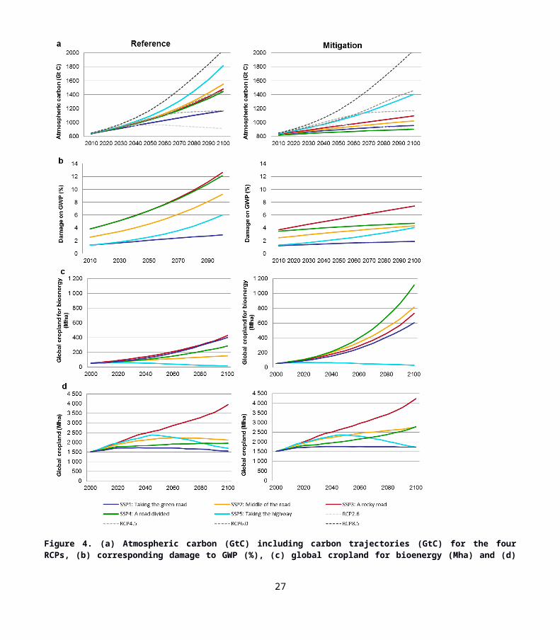
Figure 4. (a) Atmospheric carbon (GtC) including carbon trajectories (GtC) for the four RCPs, (b) corresponding damage to GWP (%), (c) global cropland for bioenergy (Mha) and (d) global cropland, including cropland for bioenergy (Mha) for reference and mitigation scenarios.

18

Only SSP1 “Taking the green road” achieves an atmospheric carbon pathway close to RCP4.5 for the reference case, while

the remaining scenarios are all clustered around RCP6.0 (Fig. 4, panel a). The introduction of a global carbon tax and the

subsequent reduction of energy use and transition towards renewable energies yield considerably lower concentration

pathways for the mitigation scenarios. SSP1 “Taking the green road” and SSP4 “A road divided” approach RCP2.6, while

SSP2 “Middle of the road” and SSP3 “A rocky road” are between RCP2.6 and RCP4.5, leaving SSP5 “Taking the highway”

with the highest mitigation concentration pathway (close to RCP6.0, Fig. 4, panel a).

If not mitigated, climate change causes damage to GWP by up to 12 % in 2100 (SSP3 “A rocky road” and SPP4 “A road

divided”, Fig. 4, panel b). For scenarios with low and medium challenges for adaptation the damage is 3-9% of GWP in

2100. Climate change mitigation strategies reduce the impact to below 8% damage to GWP in 2100 for all scenarios (Fig. 4,

panel b). The largest reduction of damage occurs for SSP4 “A road divided” (from 12% to 5% of GWP, Fig. 4 and Fig. 5)

where the low challenges for mitigation enable a strong reduction in emissions, while the high challenges for adaptation

make such reduction very desirable. Similar reasoning explains why the global carbon tax in SSP4 “A road divided” is

significantly higher than in the other scenarios. The impacts of the avoided damage in the mitigation scenarios on food

consumption, yields and cropland are presented in the next section.

The contribution of bioenergy to the total energy supply increases generally from the reference case to the mitigation case

(except SSP5 “Taking the highway”), but is especially pronounced for the mitigation scenario of SSP2 “Middle of the road”

and SSP4 “A road divided” (Fig. 3). Consequently, the global cropland area for bioenergy production increases rapidly in the

mitigation scenarios; as much as ten times for SSP4 “A road divided” between 2000 and 2100 (Fig. 4, panel c). The rapid

expansion of cropland area for bioenergy production is the main driver for increases in total global cropland area for the

mitigation scenarios of SSP2 “Middle of the road” and SSP4 “A road divided” (Fig. 4, panel d). Even for SSP1 “Taking the

green road” bioenergy production is the prevailing driver of cropland expansion. However, in this scenario the cropland

expansion for bioenergy is counteracted by the sustainable lifestyle choices (e.g., decreasing meat consumption) and strong

increases in yields, which together lead to a reduction of cropland area for food production. Quite differently, very low levels

of technological change and thus very slow yield development paired with a strongly increasing population (12.1 billion

people in 2100) result in the massive expansion of global total cropland for SSP3 “A rocky road” in both the reference and

mitigation scenariocases. The trend of expanding and stabilizing global cropland in most scenarios is contrasted by the

development of global cropland for SSP5 “Taking the highway” in which global cropland increases and peaks in the first

half of the 21st century, declining in the second half. The initial cropland expansion is due to the resource-intensive lifestyle

of a slightly growing, more affluentuch richer population, while bioenergy production does not play a role in this fossil

fuelled scenario. For SSP5 “Taking the highway” strong yield developments and a declining population with saturated food

demands lead to global cropland contraction in the second half of the 21st century.

19

5

10

15

20

25

30

3.2 Impact of mitigation on consumption, yields and cropland area

The avoided damage to GWP due to the introduction of mitigation strategies is at almost 8% in 2100 largest for SSP4 “A

road divided”, followed by SSP2 “Middle of the road” and SSP3 “A rocky road” (each around 5% in 2100, Fig. 5). The

consumption of milk and meat is dependent on income and thus higher income associated withwhich is enhanced by lower

climate-induced damage, enablinges additional consumption. For SSP3 “A road divided” the additional global average meat

consumption (due to avoided damage) is close to 1 kg meat per capita in 2100 (Fig. 5). In developing countries additional

meat consumption is up to 1.5 kg meat per capita in 2100. However, compared with uncertainties within the relationship of

income and meat consumption, as well as in lifestyle and cultural preference (e.g., for SSP3 “A rocky road” the global

average meat consumption in 2100 is 52 ± 10 (1 SD) kg meat per capita (Engström et al., 2016a), such an impact of

mitigation on per capita meat consumption appears relatively modest.

Differently to meat and milk (similar impact as for meat consumption, not shown) consumption, global average yield and

global cropland area can be affected not only by avoided damage to GWP, but also by changed bioenergy production and

yield. Each SSP’s yield is the result of weighting the yield simulated by the ecosystem model under each RCP depending on

the distance of the SSP’s concentration pathway to that RCP (see Sect. 2.2.3 and Appendix A5). For example, for to compute

the yield forof SSP2 “Middle of the road,” the ecosystem model-simulated yields underfrom RCP2.6, RCP4.5, RCP6.0 and

RCP8.5 biophysical forcing (combined with SSP2 land use and management assumptions) were weighted with 0.09, 0.15,

0.63 and 0.12 respectively (these numbers, which sum to 1.0, are called the “yield distribution”, see Appendix A5 for yield

distributions of the other scenarios). The yield distributions changes when mitigation strategies are introduced, as the

concentration pathway for each SSP is changed (Fig. 4, panel a). Due to investments in agricultural management, yield

development is assumed also to be dependent on income, and thus avoided damage to GWP can increase yields in mitigation

scenarios relative to reference scenarios.

20

5

10

15

20

Figure 5. Impact of avoided damage to GWP (% of total GWP) due to mitigation on global aggregated meat consumption in 2100 relative to 2000 for the five SSPs.

For all scenarios, the avoided damage to GWP leads to slightly larger global average yields in the mitigation scenario

compared to the reference case (up to 1%, Fig. 6, panel a). Changes in yield distributions have a stronger positive impact in

the mitigation scenario of SSP1 “Taking the green road” (almost 3%) and SSP2 “The middle of the road” (1.5%), while the

impact on yield in SSP5 “Taking the highway” is negative. Increased bioenergy production in the mitigation scenarios has a

very small impact on global average yield, as this impact is only indirect due to different allocation of cropland areas (areas

with lower or higher yields). By contrast, the increased bioenergy production is the absolute largest contributor to the

difference in global cropland area between mitigation and reference scenarios (Fig. 6, panel b). This is most strongly so for

SSP2 “Middle of the road” and SSP4 “A road divided”. Factors that resulted in larger yields in mitigation scenarios (avoided

damage and yield distribution) counteract the cropland expansion caused by the increased bioenergy production (higher

yields, less cropland expansion), though with by only a few percentage points when compared to the magnitude of the direct

impact of bioenergy on cropland expansion in mitigation scenarios.

Figure 6. (a) Difference between reference and mitigation scenarios for change in global yield between 2000 and 2100 (%) and (b) change in global cropland area between 2000 and 2100 (%). The grey bar gives the total differences (sum of differences due to damage, yield distribution and bioenergy), while the colored bars show the contribution of each causal factor to the total difference.

21

5

10

15

20

3.3 Spatially explicit cropland changes and impact on the terrestrial carbon balance

Cropland expansion in 2100 compared to 2000 (Fig. 7) can be observed in all scenarios in Sub-Saharan Africa, Brazil,

Mexico, and in the Corn Belt and the Great Plains of North America. In the reference scenarios (all except SSP3 “A rocky

road”) and also in the mitigation scenarios of SSP1 “Taking the green road” and SSP5 “Taking the highway” this cropland

expansion is paired with cropland abandonment (green areas in Fig. 7) in other parts of North and South America, as well as

in Eastern Europe and to some extent in Asia and Australia. An exception to this general pattern is SSP3 “A rocky road”,

where cropland expansion is predominant across all fertile lands globally. This is due to the combination of high population

growth with resource intensive lifestyles as well as low yield increases. In the mitigation scenario of SSP3 “A rocky road”,

bioenergy is mainly produced from crops grown in Brazil and the US (150 Mha each), but also Russia and Indonesia (50

Mha each). Even in other mitigation scenarios with large increases in cropland for bioenergy production (> 600 Mha in SSP2

and SSP4 compared to reference scenario), the increase is mainly allocated in Brazil, the US, Russia, Indonesia and to a

lesser extent in India, Canada and Australia. The same pattern of cropland allocation for bioenergy production can be

observed for the mitigation scenario of SSP1 “Taking the green road” (200 Mha more cropland for bioenergy production

compared to reference scenario). Interestingly, the very similar global aggregated cropland areas of the mitigation scenarios

of SSP1 “Taking the green road” and SSP5 “Taking the highway” in 2100 (1725 Mha and 1722 Mha respectively) are

distributed differently in the two scenarios: in SSP5 “Taking the highway” cropland changes led to more concentrated

cropland areas in e.g. Sub Saharan Africa, Central America and Russia, while in SSP1 “Taking the green road” there are

more subtle changes over larger areas, e.g. in Brazil, the US, Indonesia, but also Sub-Saharan Africa.

The large expansions of cropland areas in SSP3 “A rocky road” causes widespread carbon losses in 2100 compared to 2000,

with up to -50 kg m-2 in the tropics (Fig. 8). Even in temperate zones where cropland expands into previously forested areas,

larger carbon losses occur. Also in scenarios with comparatively modest cropland expansion compared to SSP3, terrestrial

carbon stocks decrease, especially in tropical regions and regions with cropland expansion (Fig. 7).

22

5

10

15

20

Figure 7. (a) Fraction of cropland on total land area for baseline year 2000 based on Hurrt et al. (2011). (b) Simulated cropland changes relative to baseline by 2100 for the five SSP reference (r) and mitigation (m) scenarios in the challenge for adaptation and mitigation space. Green colours indicate a decrease in cropland area in 2100 compared to 2000, while yellow and red colours indicate an increase in cropland area in 2100 compared to 2000.

Climate change leading to a longer growing season in temperature-limited high latitude ecosystems, and increases in

ecosystem productivity caused by the direct effect of rising CO2 “fertilisation”on the biochemistry of photosynthesis, have

been identified as important drivers of the carbon balance of the terrestrial land surface (Le Quéré et al., 2015; Schimel et al.,

2015), as simulated here for high latitude regions in all scenarios, and for wet tropical regions such as the Amazon and

Congo Basin in all scenarios except to some extent SSP3.

23

5

10

Figure 8. Changes in modelled total terrestrial carbon pool (kg m -2) for 2000-2100. Green to blue colours indicate an increase in the carbon pool, while yellow and purple colours indicate a decrease in carbon pool.

After aggregating the changes in the terrestrial carbon pool at theAggregated to the global scale we found that the terrestrial

biosphere is a carbon sink for most scenarios throughout the 21st century, but becomes a carbon source for scenarios with

large cropland expansion (SSP3 “A rocky road” and SSP4m “An unequal world”, Fig. 9). The global net-increase in

terrestrial carbon storage for most scenarios is not necessarily primarily driven by LULCC, but by the effects of climate

change and CO2 fertilisation (as described above). To isolate the effect of climate changethese biophysical effects on

ecosystem carbon pools in comparison to changes caused by vs. LULCC we performed simulations with constant land-use

but changing climate and CO2 (see Appendix A8, Fig. A 1). These simulations suggest that without LULCC, the global

terrestrial biosphere would act as a carbon sink for all scenarios (Appendix A8, Fig. A 1). This would be most strongly the

case for scenarios predominantly driven by high concentration pathways for atmospheric CO2 (RCP6.0 and RCP8.5, arriving

at approximately 2175 GtC in 2100), but even for scenarios driven by the low concentration pathway RCP2.6 (arriving at

approximately 2115 GtC in 2100).

24

5

10

15

LULCC erodes terrestrial C stocks for all scenarios by around 50 to 200 GtC by 2100. For SSP3 “A rocky road” the effect of

the large-scale cropland expansion outweighs the climate change-driven sequestration of terrestrial carbon and the terrestrial

biosphere turns into a net carbon source in the second half of the 21 st century. This occurs more strongly for SSP3m

compared to SSP3r, mainly due to lower assumed atmospheric CO2 concentrations in the mitigation scenario (higher

weighting of low radiative forcing RCP scenarios; Appendix A5), resulting in less CO2 fertilisation of plant production, an

eaffect expressed particularly in the simulated carbon balance of the tropics (Figs. 8,9). Production of bioenergy for

mitigation and the related increase in cropland area (> 800 Mha cropland for bioenergy production in 2100) contributes to

shifting affected areas from a carbon sink into a carbon source, as seen for SSP4m “An unequal road” (Fig.  9). In the fossil

fuelled SSP5 “Taking the highway”, bioenergy production does not increase, but the global carbon tax still reduces energy

demand through enhanced energy efficiency, resulting in lower emissions, reflected in a greater weighting towards RCP6 in

SSP5m and towards RCP8.5 in SSP5r (Appendix 5). However, the combined effects of climate, atmospheric CO 2 and land

use result in almost identical carbon trajectories for the reference and mitigation cases of SSP5 (Fig. 9). SSP1m “Taking the

green road” is the only scenario with expansion of cropland for production of bioenergy where the biosphere continues to be

a strong carbon sink through the 21st century (Fig. 9).

Figure 9: Changes in global terrestrial biosphere carbon pool (GtC) from 2000 to 2100 for all SSPs, reference (r) and mitigation (m) case. The slope indicates whether the net ecosystem carbon balance (NECB) is a carbon source (negative slope) or carbon sink (positive slope).

25

5

10

15

20

4 Discussion

4.1 Findings in the context of other studies

We present a novel IAM framework and provide an new set of consistent SSP-scenario quantifications for energy supply,

atmospheric carbon concentration, climate-induced damage to GWP and bioenergy production from energy crops, exploring

impacts on food consumption, cropland change and terrestrial carbon storage. The SSP-scenario quantifications available

from the SSP database suggest that primary energy for all five SSPs will range from 700 to 1824 EJ in 2100 for the baseline

case, and from 562 to 1316 EJ in 2100 under mitigation [considering only the marker scenarios and choosing the mitigation

scenario with the RCP that is closest to our realization, (Fig. 3; SSP-Database, 2015)]. For the mitigation scenarios, this

compares to 1087-1252 EJ of primary energy in 2100, estimated by the climate-economy model in our study. In the SSP

database quantifications, energy from biomass production increases for all baseline scenarios (differently to our projections

even for SSP5 “Taking the highway”), and is much more pronounced in the mitigation scenarios. For example, for SSP4 “A

road divided” the mitigation scenario simulated with GCAM4 (SSP4-26) projects primary energy use from biomass of 448

EJ in 2100, compared to 111 EJ in 2100 in the baseline scenario (SSP4-Baseline). This increase is comparable to thatsimilar

as in our study (reference: 191 EJ in 2100 vs. mitigation: 519 EJ in 2100) and is also accompanied by a strong increase in

cropland area due to mitigation (2936 Mha and 1761 Mha in 2100 in the mitigation and baseline case, respectively; 2777

Mha and 1962 Mha, respectively, in our study) (SSP-Database, 2015). Similarly, the CO2 emission trajectories calculated

from the climate-economy model compare with the CO2 emission trajectories reported in Riahi et al. (2017; Fig. A 2 in

Appendix A8). Cropland projections for the SSP database quantifications cover a range from 1052 to 2936 Mha, which is

slightly wider compared to the ranges previously published in the literature. For example, Schmitz et al. (2014) analysed

cropland development until 2050 for scenarios based on SSP2 “Middle of the road” and SSP3 “A rocky road”, taking into

account a range of climate projections and agro-economic models, arriving at a range from 1400 Mha to 2300 Mha in 2050.

A later model inter-comparison study (Alexander et al., 2017) including a larger set of models and scenarios (including all

five SSPs) arrived at global cropland projections of 1100 to 2700 Mha in 2100. Our cropland projections for all scenarios,

except SSP3 “A rocky road”, are within the range reported by other studies and modelling teams (1546 to 2777 Mha in

2100). Cropland projections for SSP3 “A rocky road” extend beyond this range (3950 Mha and 4237 Mha in reference and

mitigation respectively); reasons are discussed below. Biomass losses in conjunction with the extreme cropland increases

projected under this scenario provide the major explanation for terrestrial ecosystems becoming a carbon source in our

analysis.

Since pre-industrial times, LULCC has contributed 180 80 GtC or about one-third of total anthropogenic CO2 emissions,

to the atmosphere (Ciais et al., 2013). Biomass loss in conjunction with tropical deforestation is an important source, but is

compensated in part by a sink due to forest regeneration on abandoned cropland, e.g. in conjunction with agricultural

intensification in mid-latitude countries after World War II (Shevliakova et al., 2009). If LULCC effects on biosphere carbon

26

5

10

15

20

25

30

balance are disregarded, a residual carbon sink averaging 3.0 0.8 GtC yr1 for 2005-2014 (Le Quéré et al., 2015) reduces

the increase in atmospheric greenhouse gas concentrations due to anthropogenic emissions by around one quarter. Some

60% of this biospheric sink has been attributed to CO2 fertiliszation (Schimel et al., 2015), while most of the remainder may

be explained by a temperature-driven increase in growing season length in higher latitudes, enhancing vegetation

productivity and creating a temporary sink for carbon in the stems of growing trees (Ahlström et al. 2012). For the future,

our simulations suggest that for scenarios with wide-spread cropland expansion and slow agricultural intensification (SSP3

“A rocky road”) biomass loss could turn the terrestrial biosphere once again into a carbon source. LULCC has been

previously shown to influence the carbon balance simulated by LPJ-GUESS, resulting in a general increase in carbon flux to

the atmosphere under cropland expansion (Pugh et al., 2015). In all scenarios except SSP3 the residual carbon sink

outweighs LULCC-induced carbon loss and the terrestrial biosphere sequesters 1.1  0.4 GtC yr1 for 2000-2100 (or 1.9

0.3 GtC yr1 for 2000-2100 disregarding LULCC). If second generation bioenergy feedstocks were to be explicitly included

in the IAM framework, the impact of cropland expansion on the terrestrial carbon balance could be expected to be partially

mitigated by carbon-sequestering second feedstock crops, such as switch grass and woody biomass. An earlier scenario

study (based on the earlier, SRES scenario framework) suggested an average net sink of 2-6 GtC yr -1 for 1990-2100 but in

contrast to our scenarios, three of the four underlying scenarios assumed a decrease in cropland areas (Levy et al., 2004).

More recent estimates for the period 2000-2009 suggested a terrestrial carbon sink of 1.1 0.1 GtC yr1 (Houghton et al.,

2012), which is in the same range as our results for the 2000-2100 period.

The introduction of a global carbon tax as a mitigation strategy paired with the socio-economic characteristics of the SSPs

results in varying reductions in atmospheric carbon concentrations in the range spanned by RCP2.6 and RCP6.0. Scenarios

with low challenges for mitigation (SSP1 “Taking the green road”), especially when combined with high challenges for

adaptation (SSP4 “A road divided”) achieve mitigation pathways that are comparable to the stringent emissionsmitigation

trajectory ofscenario RCP2.6. However, as the imposed carbon tax only applies for fossil fuels, indirect emissions of land-

use change caused by increased bioenergy production in the mitigation scenarios are not considered in these emission

reductions. For SSP4 “A road divided”, the terrestrial biosphere becomes a source of carbon in the second half of the 21st

century and makes it unlikely that SSP4 “A road divided” truly achieves a concentration pathway comparable to RCP2.6. By

contrast, if socio-economic conditions – such as environmentally-conscious life-style choices (low-meat diet) paired with

low population increase and strong technological growth – enable the reduction of cropland needed for food production,

bioenergy from energy crops can be produced on the abandoned food-cropland and the biosphere as a whole acts as a sink,

as for SSP1 “Taking the green road”. This supports previous studies (Erb et al., 2012; Haberl et al., 2011; Kraxner et al.,

2013) that point out that only under specific conditions is bioenergy production sustainable and can contribute to mitigation

of climate change.

In context with the mitigation strategies it is remarkable that the introduction of only 10% of the optimal carbon tax leads to

significant energy, and thus atmospheric carbon concentration, reductions (e.g. SSP3 “A rocky road”, 35% energy reduction

and 26% atmospheric carbon concentration reduction compared to reference scenario in 2100). Thus, if high damages are

27

5

10

15

20

25

30

expected (as in SSP3 “A rocky road”) even the introduction of a carbon tax that is far from optimal is a surprisingly effective

strategy to mitigate climate change. However, this is under the assumption that the global carbon tax is introduced

immediately and no further delays in climate change mitigation occur. Due to inertia in the climate system, the early

reduction of GHG emissions is crucial for the long-term effectiveness of any mitigation strategy (Luderer et al., 2013), but

this is a very large challenge for the global community. Thus, especially for scenarios with high challenges for mitigation,

the reductions in atmospheric carbon due to reduced fossil fuel consumption suggested by our study are on the optimistic

side of available estimates. In comparison, the SPAs that accompany the SSP marker scenarios assume specifically different

lengths of transition phases until full global climate cooperation is reached (and transition towards a globally uniform carbon

price thereafter), where the most ambitious SPA assumes complete transition by 2020 and is only used for SSPs with low

challenges for mitigation (Riahi et al., 2015). A second key assumption in the SPAs concerns the extent of land-based

mitigation. For examples, for SSPs with high affluence and high equality (SSP1 “Taking the green road” and SSP5 “Taking

the highway”) it is assumed in the SPAs that all land use emissions are taxed with the same level of carbon prices as in the

energy sector (Riahi et al., 2015). In our study, the mitigation scenario for SSP5 “Taking the highway” achieves a

concentration pathway just below RCP6. To reach a more stringent RCP, such as RCP2.6, land-based mitigation options

would need to be considered, such as afforestation projects or carbon capture and storage (see Sect. 4.3 for further

discussion). Previous studies suggest that eExcluding emissions from land-use in mitigation strategies wouldhas previously

been observed to lead to large scale land-use change (Wise et al., 2009), as simulated here for SSP2 “Middle of the road”

and SSP4 “A road divided”. Further, only taxing fossil fuels leads to unintended outcomes, such as the higher total energy

consumption in the mitigation scenario for SSP1 “Taking the green road” compared to the reference scenario for SSP1.

4.2 Uncertainties in the IAM framework and input data

The presented scenario outcomes should be treated as illustrative, as a wide range of outcomes can arise due to uncertainties

in interpretations and quantification of scenario assumptions (Engström et al., 2016a). For example, the uncertainty range for

one scenario of cropland change was 1330-1750 Mha by 2100 from 1500 Mha in 2000 (1SD, Engström et al., 2016a).

Differences in model structure can likewise cause large spread in results. For example, using one scenario, but 10 different

models, Schmitz et al. (2014) projected cropland changes ranging from 1400-2000 Mha by 2050 (relative to a baseline of

1500 Mha in 2000), depending on the model chosen (despite harmonized input data). Differences were related to diverse

model assumptions as to land availability, costs for land conversion and endogenous yield responses to technological change

(Schmitz et al., 2014). Similarly, the future fate of the net biospheric sink for carbon is highly uncertain, with biospheric

models projecting divergent trajectories in net carbon balance depending on the increase in atmospheric CO2 associated with

a given emissions scenario (e.g. RCP), the climate patterns and trends projected by different GCMs in response to the

emissions, differences in ecosystem response simulated by different biosphere models, and whether or not biogeochemical

and biophysical biosphere-atmosphere feedbacks are taken into account (Ahlström et al., 2012; Boysen et al., 2014; Cramer

et al., 2001; Friedlingstein et al., 2014; Sitch et al., 2008). The IPSL climate model chosen to provide climatic forcing for the

28

5

10

15

20

25

30

ecosystem model simulations in our study induces carbon cycle changes in the middle of the range of an ensemble forced by

multiple GCMs (Ahlström et al., 2012, Fig. A 3 in Appendix A.8). Another example of the importance of model structure is

the simulated cropland change for SSP3 “A rocky road” of 3950 Mha in reference scenario, compared to an earlier

quantification of SSP3 “A rocky road” with a mean of 2280 Mha with identical parameter settings, but an earlier version of

the land-use model used here (Engström et al., 2016a). The structural changes in the updated model version are related to the

intensification of the livestock sectors, the trade mechanism, and bioenergy production. Previously, the trade mechanism

allowed substantial underproduction, which was assumed to be avoided in the updated model version. Thus, the increased

demand (11% higher cereal demand due to allowed intensification of the livestock sector and 15.2 EJ bioenergy from crops

in 2100 in SSP3 “A rocky road”), paired with the fulfilment of demand, leads to the very high cropland projections for SSP3

“A rocky road”. The cropland expansion in SSP3 is further driven by very low global average yield increase (3.2 ton ha -1 in

2100 and 3.0 ton ha-1 in 2000, compared to 5.2 ton ha-1 in 2100 for SSP5 “Taking the highway”), which is partly also caused

by the damage to GWP and thus reduced investments in agricultural technologies.

Additionally to uncertainty arising from model structure, different interpretations of scenarios as well as the translation of

qualitative scenario information into quantitative scenario parameterizations contribute to uncertainties of scenario

outcomes. For the land-use model used here, the effect of uncertainties in input parameters was shown to produce scenario

outcomes with uncertainty ranges (2 × SD) of up to 27% of the scenario mean (Engström et al., 2016a). For the outcome of

the climate-economy model uncertainties arise especially due to parameter interdependencies of substitution elasticity with

increase in growth rates for fossil fuels and clean energy. Slightly different parameter combinations can lead to very different

outcomes. Other parameters, such as the discount rate, were not varied here, but likewise have the potential to change model

outcomes (Golosov et al., 2014).

However, the relative similarity of our results to the public SSP quantifications (Riahi et al., 2017; SSP-Database, 2015)

gives us confidence that our projections are plausible both in the direction and magnitude of change and can serve as

examples for the quantification of the SSPs based on a coherent logic.

4.3 Limitation of the study and further research

One limitation of the presented study already alluded to is the restriction of the mitigation strategies to the energy sector. It

would be a valuable addition to the modelling framework to include other land based mitigation strategies, e.g. avoided

deforestation and afforestation, as well as demand-side mitigation strategies (meat-low diets, reduction of food waste) which

have been previously shown to have a great mitigation potential (Smith et al., 2013). In the current study bioenergy

production is limited to first-generation bioenergy crops. In future work, it would be desirable to introduce second generation

bioenergy feedstocks that are shown to have greater high mitigation potential, such as C4 grasses and switch-grass (Albanito

et al., 2016). Additionally, the information flow within the IAM framework could be improved. One such improvement

would be to inform theconnect emissions in the climate-economy model toabout land-use based emissions due to bioenergy

production derived from the ecosystem model. The assumption that clean energy (of which bioenergy is one part) is free

29

5

10

15

20

25

30

from emissions should then be revised or bioenergy modelled as a separate energy source. Further research could also

improve the treatment of the uncertainties outlined above. A systematic sensitivity study of the climate-economy model

paired with a sensitivity study performed earlier for the land-use model (Engström et al., 2016a) would give better insights

into the impact of energy mitigation strategies on consumption, yield and cropland. Also, the impact of cropland changes and

mitigation-derived reduced climate change on the terrestrial carbon balance could be quantified with an ensemble of GCMs

to account for the uncertainties in climate forcing arising from structural differences among GCMs.

The carbon cycle simulations were performed with dynamically evolving climate and land cover inputs only, while cropland

management was kept at the 2006 level. This could affect the results, but enhanced productivity due to fertilisation and

irrigation would, to some degree, be balanced by an increase in soil decomposition, so the resultant uncertainty in terms of

biosphere carbon balance may be minor in relation to other uncertainties.

5 Conclusions

Our results suggest that the indirect impacts of climate mitigation strategies on global cropland are small in comparison to

impacts due to the spread of bioenergy production and other sources of uncertainties, such as model structure and

uncertainties in parameterizations. We found that different drivers, such as food production vs. bioenergy production, can

lead to contrasting land-use change patterns, as observed here for SSP1 “Taking the green road” and SSP5 “Taking the

highway”. Further, without substantial increases in global average crop yields, feeding the global population of 12.1 billion

in 2100 assumed under SSP3 “A rocky road”, additionally to producing bioenergy, will cause serious deforestation and

transforms the global terrestrial biosphere from a sink to an additional carbon pool to a sink source of carbon emissions to

the atmosphere. Our study thus underlines previous assertions that bioenergy production from energy crops is only a

sustainable mitigation strategy if other socio-economic factors, such as population growth, technological change and lifestyle

choices, free up existing cropland areas for allocation to bioenergy production.

Acknowledgments

We acknowledge funding from the Formas Strong Research Environment grant “Land use today and tomorrow” (LUsTT;

dnr: 211-2009-1682) and the Swedish Research Programme for Climate, Impacts and Adaptation (SWECIA) funded by the

Foundation for Strategic Environmental Research (Mistra). Peter Alexander is thanked for supply of initial values of

bioenergy production, calculated from FAOSTAT (2015). This study is a contribution to the Strategic Research Area

Biodiversity and Ecosystem Services in a Changing Climate (BECC).

30

5

10

15

20

25

References

Ahlström, A., Schurgers, G., Arneth, A., Smith, B. (2012) Robustness and uncertainty in terrestrial ecosystem carbon

response to CMIP5 climate change projections. Environmental Research Letters 7, 044008.

Albanito, F., Beringer, T., Corstanje, R., Poulter, B., Stephenson, A., Zawadzka, J., Smith, P. (2016) Carbon implications of

converting cropland to bioenergy crops or forest for climate mitigation: a global assessment. GCB Bioenergy 8, 81-95.

Alexander, P., Rounsevell, M.D.A., Dislich, C., Dodson, J.R., Engström, K., Moran, D. (2015) Drivers for global

agricultural land use change: The nexus of diet, population, yield and bioenergy. Global Environmental Change 35, 138-147.

Alexander, P., Prestele, R., Verburg, P.H., Arneth, A., Fujimori, S., Hasegawa, T., Jain, A.K., Meiyappan, P., Dunford, R.,

Harrison, P.A., Brown, C., Holzhauer, S., Dendoncker, N., Steinbuks, J., Lenton, T., Powell, T., Sands, R.D., Kyle, P., Wise,

M.A., Doelman, J., Stehfest, E., Schaldach, R., Jacobs-Crisioni, C., Lavalle, C., van Meijl, H., Tabeau, A., Humpenöder, F.,

Popp, A., Engström, K., Butler, A., Liu, J., Rounsevell, M. (2017) Assessing uncertainties in future land cover projections.

Global Change Bioloy 23, 767-781.

Boysen, L.R., Brovkin, V., Arora, V.K., Cadule, P., de Noblet-Ducoudré, N., Kato, E., Pongratz, J., Gayler, V. (2014)

Global and regional effects of land-use change on climate in 21st century simulations with interactive carbon cycle. Earth

System Dynamics 5, 309-319.

Bruckner, T., Bashmakov, I.A., Mulugetta, Y., Chum, H., de la Vega Navarro, A., Edmonds, J., Faaij, A., Fungtammasan,

B., Garg, A., Hertwich, E., Honnery, D., Infield, D., Kainuma, M., Khennas, S., Kim, S., Nimir, H.B., Riahi, K., Strachan,

N., Wiser, R., Zhang, X. (2014) Energy Systems. In: Climate Change 2014: Mitigation of Climate Change. Contribution of

Working Group III to the Fifth Assessment Report of the Intergovernmental Panel on Climate Change [Edenhofer, O., R.

Pichs-Madruga, Y. Sokona, E. Farahani, S. Kadner, K. Seyboth, A. Adler, I. Baum, S. Brunner, P. Eickemeier, B. Kriemann,

J. Savolainen, S. Schlömer, C. von Stechow, T. Zwickel and J.C. Minx (eds.)]. Cambridge University Press, Cambridge,

United Kingdom and New York, NY, USA.

Börjesson, P., Tufvesson, L.M. (2011) Agricultural crop-based biofuels – resource efficiency and environmental

performance including direct land use changes. Journal of Cleaner Production 19, 108-120.

Canadell, J.G., Schulze, E.D. (2014) Global potential of biospheric carbon management for climate mitigation. Nature

Communications 5, 5282.

Ciais, P., Sabine, C., Bala, G., Bopp, L., Brovkin, V., Canadell, J., Chhabra, A., DeFries, R., Galloway, J., Heimann, M.,

Jones, C., LeQuere, C., Myneni, R.B., Piao, S., Thornton, P. (2013) Carbon and other biogeochemical cycles, in: Climate

Change 2013: The Physical Science Basis. Contribution of Working Group I to the Fifth Assessment Report of the

Intergovernmental Panel on Climate Change, edited by: Stocker, T. F., Qin, D., Plattner, G.-K., Tignor, M., Allen, S. K.,

Boschung, J., Nauels, A., Xia, Y., Bex, V., and Midgley, P. M., Cambridge University Press, Cambridge, UK and New

York, NY, USA. 465–570.

31

5

10

15

20

25

30

Cramer, W., Bondeau, A., Woodward, F.I., Prentice, I.C., Betts, R.A., Brovkin, V., Cox, P.M., Fisher, V., Foley, J.A.,

Friend, A.D., Kucharik, C., Lomas, M.R., Ramankutty, N., Sitch, S., Smith, B., White, A., Young-Molling, C. (2001) Global

response of terrestrial ecosystem structure and function to CO2 and climate change: results from six dynamic global

vegetation models. Global Change Biology 7, 357-373.

Donner, L.J., Wyman, B.L., Hemler, R.S., Horowitz, L.W., Ming, Y., Zhao, M., Golaz, J.-C., Ginoux, P., Lin, S.-J.,

Schwarzkopf, M.D., Austin, J., Alaka, G., Cooke, W.F., Delworth, T.L., Freidenreich, S.M., Gordon, C.T., Griffies, S.M.,

Held, I.M., Hurlin, W.J., Klein, S.A., Knutson, T.R., Langenhorst, A.R., Lee, H.-C., Lin, Y., Magi, B.I., Malyshev, S.L.,

Milly, P.C.D., Naik, V., Nath, M.J., Pincus, R., Ploshay, J.J., Ramaswamy, V., Seman, C.J., Shevliakova, E., Sirutis, J.J.,

Stern, W.F., Stouffer, R.J., Wilson, R.J., Winton, M., Wittenberg, A.T., Zeng, F. (2011) The Dynamical Core, Physical

Parameterizations, and Basic Simulation Characteristics of the Atmospheric Component AM3 of the GFDL Global Coupled

Model CM3. Journal of Climate 24, 3484-3519.

Dufresne, J.L., Foujols, M.A., Denvil, S., Caubel, A., Marti, O., Aumont, O., Balkanski, Y., Bekki, S., Bellenger, H.,

Benshila, R., Bony, S., Bopp, L., Braconnot, P., Brockmann, P., Cadule, P., Cheruy, F., Codron, F., Cozic, A., Cugnet, D., de

Noblet, N., Duvel, J.P., Ethé, C., Fairhead, L., Fichefet, T., Flavoni, S., Friedlingstein, P., Grandpeix, J.Y., Guez, L.,

Guilyardi, E., Hauglustaine, D., Hourdin, F., Idelkadi, A., Ghattas, J., Joussaume, S., Kageyama, M., Krinner, G.,

Labetoulle, S., Lahellec, A., Lefebvre, M.P., Lefevre, F., Levy, C., Li, Z.X., Lloyd, J., Lott, F., Madec, G., Mancip, M.,

Marchand, M., Masson, S., Meurdesoif, Y., Mignot, J., Musat, I., Parouty, S., Polcher, J., Rio, C., Schulz, M., Swingedouw,

D., Szopa, S., Talandier, C., Terray, P., Viovy, N., Vuichard, N. (2013) Climate change projections using the IPSL-CM5

Earth System Model: from CMIP3 to CMIP5. Climate Dynamics 40, 2123-2165.

Engström, K., Olin, S., Rounsevell, M.D.A., Brogaard, S., van Vuuren, D.P., Alexander, P., Murray-Rust, D., Arneth, A.

(2016a) Assessing uncertainties in global cropland futures using a conditional probabilistic modelling framework. Earth

System Dynamics Discussions, 1-33.

Engström, K., Rounsevell, M.D.A., Murray-Rust, D., Hardacre, C., Alexander, P., Cui, X., Palmer, P.I., Arneth, A. (2016b)

Applying Occam's razor to global agricultural land use change. Environmental Modelling & Software 75, 212-229.

Erb, K.-H., Haberl, H., Plutzar, C. (2012) Dependency of global primary bioenergy crop potentials in 2050 on food systems,

yields, biodiversity conservation and political stability. Energy Policy 47, 260-269.

FAO/IIASA (2011) Global Agro-ecological Zones (GAEZ v3.0). FAO Rome, Italy and IIASA, Laxenburg, Austria.

FAOSTAT (2015) Commodity Balances/Crops Primary Equivalent (2015-12-16). Food and Agriculture Organization of the

United Nations, Rome, Italy.

FAOSTAT (2016) Production and Food Balance data (2016-01-21). Food and Agriculture Organization of the United

Nations, Rome, Italy.

Fargione, J., Hill, J., Tilman, D., Polasky, S., Hawthorne, P. (2008) Land Clearing and the Biofuel Carbon Debt. Science

319, 1235-1238.

32

5

10

15

20

25

30

Friedlingstein, P., Meinshausen, M., Arora, V.K., Jones, C.D., Anav, A., Liddicoat, S.K., Knutti, R. (2014) Uncertainties in

CMIP5 Climate Projections due to Carbon Cycle Feedbacks. Journal of Climate 27, 511-526.

Golosov, M., Hassler, J., Krusell, P., Tsyvinski, A. (2014) Optimal Taxes on Fossil Fuel in General Equilibrium.

Econometrica 82, 41-88.

Fuss, S., Canadell, J. G., Peters, G. P., Tavoni, M., Andrew, R. M., Ciais, P., Jackson, R. B., Jones, C. D., Kraxner, F.,

Nakicenovic, N., Le Quéré, C., Raupach, M. R., Sharifi, A., Smith, P., and Yamagata, Y. (2014) Betting on negative

emissions, Nature Climate Change, 4, 850-853.

Haberl, H., Beringer, T., Bhattacharya, S.C., Erb, K.-H., Hoogwijk, M. (2010) The global technical potential of bio-energy

in 2050 considering sustainability constraints. Current Opinion in Environmental Sustainability 2, 394-403.

Haberl, H., Erb, K.-H., Krausmann, F., Bondeau, A., Lauk, C., Müller, C., Plutzar, C., Steinberger, J.K. (2011) Global

bioenergy potentials from agricultural land in 2050: Sensitivity to climate change, diets and yields. Biomass and Bioenergy

35, 4753-4769.

Hassler, J., Krusell, P., Nycander J. (2016 a) Climate Policy. Economic Policy 31:87, 505-58

Hassler, J., Krusell, P., Olovsson, C. (under review) Directed technical change as a response to natural-resource scarcity.

Hassler, J. Sinn, H.-W. (2016b) The Fossil Episode. Journal of Monetary Economics, 83, 14-26.

Houghton, R.A., House, J.I., Pongratz, J., van der Werf, G.R., DeFries, R.S., Hansen, M.C., Le Quéré, C., Ramankutty, N.

(2012) Carbon emissions from land use and land-cover change. Biogeosciences 9, 5125-5142.

Hurtt, G.C., Chini, L.P., Frolking, S., Betts, R.A., Feddema, J., Fischer, G., Fisk, J.P., Hibbard, K., Houghton, R.A., Janetos,

A., Jones, C.D., Kindermann, G., Kinoshita, T., Klein Goldewijk, K., Riahi, K., Shevliakova, E., Smith, S., Stehfest, E.,

Thomson, A., Thornton, P., Vuuren, D.P., Wang, Y.P. (2011) Harmonization of land-use scenarios for the period 1500–

2100: 600 years of global gridded annual land-use transitions, wood harvest, and resulting secondary lands. Climatic Change

109, 117-161.

IPCC (2014a) Climate Change 2014: Synthesis Report. Contribution of Working Groups I, II and III to the Fifth Assessment

Report of the Intergovernmental Panel on Climate Change [Core Writing Team, R.K. Pachauri and L.A. Meyer (eds.)].

IPCC, Geneva, Switzerland, 151 pp.

IPCC (2014b) Summary for Policymakers. In: Climate Change 2014: Mitigation of Climate Change.

Contribution of Working Group III to the Fifth Assessment Report of the Intergovernmental Panel on Climate Change

[Edenhofer, O., R. Pichs-Madruga, Y. Sokona, E. Farahani, S. Kadner, K. Seyboth, A. Adler, I. Baum, S. Brunner, P.

Eickemeier, B. Kriemann, J. Savolainen, S. Schlömer, C. von Stechow, T. Zwickel and J.C. Minx (eds.)]. Cambridge

University Press, Cambridge, United Kingdom and New York, NY, USA.

Kraxner, F., Nordström, E.-M., Havlík, P., Gusti, M., Mosnier, A., Frank, S., Valin, H., Fritz, S., Fuss, S., Kindermann, G.,

McCallum, I., Khabarov, N., Böttcher, H., See, L., Aoki, K., Schmid, E., Máthé, L., Obersteiner, M. (2013) Global

bioenergy scenarios – Future forest development, land-use implications, and trade-offs. Biomass and Bioenergy 57, 86-96.

33

5

10

15

20

25

30

Kriegler, E., Edmonds, J., Hallegatte, S., Ebi, K.L., Kram, T., Riahi, K., Winkler, H., van Vuuren, D.P. (2014) A new

scenario framework for climate change research: the concept of shared climate policy assumptions. Climatic Change 122,

401-414.

Lamarque, J.-F., Kyle, G.P., Meinshausen, M., Riahi, K., Smith, S.J., van Vuuren, D.P., Conley, A.J., Vitt, F. (2011) Global

and regional evolution of short-lived radiatively-active gases and aerosols in the Representative Concentration Pathways.

Climatic Change 109, 191-212.

Le Quéré, C., Moriarty, R., Andrew, R.M., Peters, G.P., Ciais, P., Friedlingstein, P., Jones, S.D., Sitch, S., Tans, P., Arneth,

A., Boden, T.A., Bopp, L., Bozec, Y., Canadell, J.G., Chini, L.P., Chevallier, F., Cosca, C.E., Harris, I., Hoppema, M.,

Houghton, R.A., House, J.I., Jain, A.K., Johannessen, T., Kato, E., Keeling, R.F., Kitidis, V., Klein Goldewijk, K., Koven,

C., Landa, C.S., Landschützer, P., Lenton, A., Lima, I.D., Marland, G., Mathis, J.T., Metzl, N., Nojiri, Y., Olsen, A., Ono,

T., Peng, S., Peters, W., Pfeil, B., Poulter, B., Raupach, M.R., Regnier, P., Rödenbeck, C., Saito, S., Salisbury, J.E.,

Schuster, U., Schwinger, J., Séférian, R., Segschneider, J., Steinhoff, T., Stocker, B.D., Sutton, A.J., Takahashi, T., Tilbrook,

B., van der Werf, G.R., Viovy, N., Wang, Y.P., Wanninkhof, R., Wiltshire, A., Zeng, N. (2015) Global carbon budget 2014.

Earth System Science Data 7, 47-85.

Levy, P.E., Cannell, M.G.R., Friend, A.D. (2004) Modelling the impact of future changes in climate, CO2 concentration and

land use on natural ecosystems and the terrestrial carbon sink. Global Environmental Change 14, 21-30.

Lindeskog, M., Arneth, A., Bondeau, A., Waha, K., Seaquist, J., Olin, S., Smith, B. (2013) Implications of accounting for

land use in simulations of ecosystem carbon cycling in Africa. Earth System Dynamics 4, 385-407.

Luderer, G., Pietzcker, R.C., Bertram, C., Kriegler, E., Meinshausen, M., Edenhofer, O. (2013) Economic mitigation

challenges: how further delay closes the door for achieving climate targets. Environmental Research Letters 8, 034033.

Mitchell, T.D., Jones, P.D. (2005) An improved method of constructing a database of monthly climate observations and

associated high-resolution grids. International Journal of Climatology 25, 693-712.

Nordhaus, W. (2007) To Tax or Not to Tax: The Case for a Carbon Tax. Review of Environmental Economics and Policy 1,

26-44.

Nordhaus, W. (2008) A Question of Balance: Weighing the Options on Global Warming Policies. New Haven, CT: Yale

University Press.

O’Neill, B.C., Kriegler, E., Ebi, K.L., Kemp-Benedict, E., Riahi, K., Rothman, D.S., van Ruijven, B.J., van Vuuren, D.P.,

Birkmann, J., Kok, K., Levy, M., Solecki, W. (2017) The roads ahead: Narratives for shared socioeconomic pathways

describing world futures in the 21st century. Global Environmental Change 42, 169-180.

O’Neill, B.C., Kriegler, E., Riahi, K., Ebi, K.L., Hallegatte, S., Carter, T.R., Mathur, R., van Vuuren, D.P. (2013) A new

scenario framework for climate change research: the concept of shared socioeconomic pathways. Climatic Change 122, 387-

400.

OECD/IEA, (2012) WORLD ENERGY OUTLOOK 2012. International Energy Agency, Paris.

34

5

10

15

20

25

30

Olin, S., Schurgers, G., Lindeskog, M., Wårlind, D., Smith, B., Bodin, P., Holmér, J., Arneth, A. (2015) Modelling the

response of yields and tissue C : N to changes in atmospheric CO₂ and N management in the main wheat

regions of western Europe. Biogeosciences 12, 2489-2515.

Peters, G.P., Andrew, R.M., Boden, T., Canadell, J.G., Ciais, P., Le Quéré, C., Marland, G., Raupach, M.R., Wilson, C.

(2012) The challenge to keep global warming below 2 °C. Nature Climate Change 3, 4-6.

Portmann, F.T., Siebert, S., Döll, P. (2010) MIRCA2000-Global monthly irrigated and rainfed crop areas around the year

2000: A new high-resolution data set for agricultural and hydrological modeling. Global Biogeochemical Cycles 24, n/a-n/a.

Pugh, T.A.M., Arneth, A., Olin, S., Ahlström, A., Bayer, A.D., Klein Goldewijk, K., Lindeskog, M., Schurgers, G. (2015)

Simulated carbon emissions from land-use change are substantially enhanced by accounting for agricultural management.

Environmental Research Letters 10, 124008.

Riahi, K., van Vuuren, D., Kriegler, E., Calvin, K., Fujimori, S., Emmerling, J., (2015) Integrated Assessment Modeling of

Shared Socio Economic Pathways – Study protocol for IAM runs.

Riahi, K., van Vuuren, D. P., Kriegler, E., Edmonds, J., O’Neill, B. C., Fujimori, S., Bauer, N., Calvin, K., Dellink, R.,

Fricko, O., Lutz, W., Popp, A., Cuaresma, J. C., Kc, S., Leimbach, M., Jiang, L., Kram, T., Rao, S., Emmerling, J., Ebi, K.,

Hasegawa, T., Havlik, P., Humpenöder, F., Da Silva, L. A., Smith, S., Stehfest, E., Bosetti, V., Eom, J., Gernaat, D., Masui,

T., Rogelj, J., Strefler, J., Drouet, L., Krey, V., Luderer, G., Harmsen, M., Takahashi, K., Baumstark, L., Doelman, J. C.,

Kainuma, M., Klimont, Z., Marangoni, G., Lotze-Campen, H., Obersteiner, M., Tabeau, A., and Tavoni, M.: The Shared

Socioeconomic Pathways and their energy, land use, and greenhouse gas emissions implications: An overview, Global

Environmental Change, 42, 153-168, 2017.

Schimel, D., Stephens, B.B., Fisher, J.B. (2015) Effect of increasing CO2 on the terrestrial carbon cycle. PNAS 112, 436–

441.

Schmitz, C., van Meijl, H., Kyle, P., Nelson, G.C., Fujimori, S., Gurgel, A., Havlik, P., Heyhoe, E., d'Croz, D.M., Popp, A.,

Sands, R., Tabeau, A., van der Mensbrugghe, D., von Lampe, M., Wise, M., Blanc, E., Hasegawa, T., Kavallari, A., Valin,

H. (2014) Land-use change trajectories up to 2050: insights from a global agro-economic model comparison. Agricultural

Economics 45, 69-84.

Shevliakova, E., Pacala, S.W., Malyshev, S., Hurtt, G.C., Milly, P.C.D., Caspersen, J.P., Sentman, L.T., Fisk, J.P., Wirth, C.,

Crevoisier, C. (2009) Carbon cycling under 300 years of land use change: Importance of the secondary vegetation sink.

Global Biogeochemical Cycles 23, n/a-n/a.

Sitch, S., Huntingford, C., Gedney, N., Levy, P.E., Lomas, M., Piao, S.L., Betts, R., Ciais, P., Cox, P., Friedlingstein, P.,

Jones, C.D., Prentice, I.C., Woodward, F.I. (2008) Evaluation of the terrestrial carbon cycle, future plant geography and

climate-carbon cycle feedbacks using five Dynamic Global Vegetation Models (DGVMs). Global Change Biology 14, 2015-

2039.

35

5

10

15

20

25

30

Smith, B., Perentice, I.C., Sykes, M.T. (2001) Representation of vegetation dynamics in the modelling of terrestrial

ecosystems: comparing two contrasting approaches within European climate space. Global Ecology and Biogeography 10,

621-637.

Smith, B., Wårlind, D., Arneth, A., Hickler, T., Leadley, P., Siltberg, J., Zaehle, S. (2014) Implications of incorporating N

cycling and N limitations on primary production in an individual-based dynamic vegetation model. Biogeosciences 11,

2027-2054.

Smith, P., Haberl, H., Popp, A., Erb, K.-h., Lauk, C., Harper, R., Tubiello, F.N., de Siqueira Pinto, A., Jafari, M., Sohi, S.,

Masera, O., Böttcher, H., Berndes, G., Bustamante, M., Ahammad, H., Clark, H., Dong, H., Elsiddig, E.A., Mbow, C.,

Ravindranath, N.H., Rice, C.W., Robledo Abad, C., Romanovskaya, A., Sperling, F., Herrero, M., House, J.I., Rose, S.

(2013) How much land-based greenhouse gas mitigation can be achieved without compromising food security and

environmental goals? Global Change Biology 19, 2285-2302.

SSP-Database, (2015) SSP Public Database (Version 1.1), available at:https://tntcat.iiasa.ac.at/SspDb, last access: 4 April 2017.Taylor, K.E., Stouffer, R.J., Meehl, G.A. (2012) An Overview of CMIP5 and the Experiment Design. Bulletin of the

American Meteorological Society 93, 485-498.

Tubiello, F.N., Salvatore, M., Ferrara, A.F., House, J., Federici, S., Rossi, S., Biancalani, R., Condor Golec, R.D., Jacobs, H.,

Flammini, A., Prosperi, P., Cardenas-Galindo, P., Schmidhuber, J., Sanz Sanchez, M.J., Srivastava, N., Smith, P. (2015) The

Contribution of Agriculture, Forestry and other Land Use activities to Global Warming, 1990-2012. Global Change Biology

21, 2655-2660.

Watanabe, M., Suzuki, T., O’ishi, R., Komuro, Y., Watanabe, S., Emori, S., Takemura, T., Chikira, M., Ogura, T.,

Sekiguchi, M., Takata, K., Yamazaki, D., Yokohata, T., Nozawa, T., Hasumi, H., Tatebe, H., Kimoto, M. (2010) Improved

Climate Simulation by MIROC5: Mean States, Variability, and Climate Sensitivity. Journal of Climate 23, 6312-6335.

Wise, M., Calvin, K., Thomson, A., Clarke, L., Bond-Lamberty, B., Sands, R., Smith, S.J., Janetos, A., Edmonds, J. (2009)

Implications of Limiting CO2 Concentrations for Land Use and Energy. Science 324, 1183-1186.

Yukimoto, S., Adachi, Y., Hosaka, M., Sakami, T., Yoshimura, H., Hirabara, M., Tanaka, T.Y., Shindo, E., Tsujino, H.,

Deushi, M., Mizuta, R., Yabu, S., Obata, A., Nakano, H., Koshiro, T., Ose, T., Kitoh, A. (2012) A New Global Climate

Model of the Meteorological Research Institute: MRI-CGCM3 –Model Description and Basic Performance–. Journal of the

Meteorological Society of Japan 90A, 23-64.

Zaehle, S., Friedlingstein, P., Friend, A.D. (2010) Terrestrial nitrogen feedbacks may accelerate future climate change.

Geophysical Research Letters 37, n/a-n/a.

36

5

10

15

20

25

30

Appendix

A1. PLUM development

In the earlier published version of the land use model (Engström et al, 2016a) it was assumed that the feed ratio would be

constant at year 2000 levels, resulting in potential underestimation of the feed demand for scenarios where meat and milk

consumption increase strongly, given the assumption that with increased consumption of animal products the production

intensifies, leading to a higher demand for cereal feed. In the PLUM version used here it is assumed that feed ratio increases

proportionally to the increase in consumption of animal production (half the growth), up but maximal to a scenario-specific

feed ratio maximum (5_feedRatioCap). Country level data of the feed ratio and per capita meat consumption from the year

2000 (FAOSTAT, 2016), show that only very few countries have feed ratios that exceed 0.4 (independent from per capita

meat consumption). For countries with feed ratios of 0.4 or lower the data suggest a weak correlation (R2=0.14) with per

capita meat consumption. As this relationship is quite weak, we made a conservative assumption and chose values of 0.1,

0.2, 0.1, 0.2 and 0.3 for the 5_feeedRatioCap scenario parameter for the SSP1-5 respectively.

The estimates of potential arable land were updated using the areas classified as moderate to very high suitability for high

input level rain-fed cereals (Suitability and Potential Yield) by the Agro-ecological Zones Data Portal (FAO/IIASA, 2011),

compared to the previous PLUM version (Engström et al, 2016a).

A2. Downscaling GWP

The damage to GWP was distributed among countries based on their share of Gross Domestic Product (GDP) on GWP. In

this case the burden of climate-change induced damage to GWP is divided equally. However, to ensure consistency with the

social equity assumption in the SSP scenarios, two alternative approaches were implemented. First, for scenarios with high

social equity we assumed that high income countries (HICs) would pay a larger share, i.e. 80%, of the damage, while 20%

would be paid by middle income countries (MICs) and none by low income countries (LICs). Second and vice versa, in

scenarios with limited social equity low income countries would need to pay 50% of costs, middle income 40% and high

income only 10% of costs. The reasoning in the second alternative is that low income countries are the most vulnerable to

the impacts of climate change, but would not receive much support by high income countries to deal with the consequences

of climate change. Categorization of countries into high, middle and low income countries is based on the baseline year 2000

and countries in these income groups contribute with 63%, 29% and 8% respectively to GWP in 2000 (Table A. 1, Baseline).

37

5

10

15

20

25

Table A. 1. Percentages of GWP of high, medium and low income countries for reference scenarios without downscaled damage (woD) and with downscaled damage (wD) for baseline year 2000 and in 2100.

Scenario (equity)HIC MIC LIC

woD wD woD wD woD wD

Baseline 63 63 29 29 8 8

SSP1 (high) 23 21 35 36 41 43

SSP2 (medium) 22 22 38 38 40 40

SSP3 (low) 20 21 45 46 35 33

SSP4 (medium) 33 33 41 41 26 26

SSP5 (high) 30 26 32 33 38 41

Throughout the 21st century for all scenarios the share of HICs decreases and shares of MIC and LIC countries increases

(Table A. 1). Our assumptions for the distribution of damage reinforce this pattern for scenarios with high equity, while the

pattern is weakened in scenarios with low equity, see Table A. 1.

A3. Clean energy to bioenergy

Clean energy projections (nuclear and renewable energies) from the climate-economy model were disaggregated to receive

bioenergy projections by a) converting energy from climate-economy model from Gtoe into EJ, multiply with 41.868 (1

Gtoe = 41.868 EJ); b) calculating nuclear energy by multiplying the total energy from the climate-economy model (oil, coal,

clean energy) with the share of nuclear energy from the WEO scenarios (see Table A. 2); and c) calculating bioenergy by

subtracting nuclear energy from clean energy (= total renewable energies) and multiplying with the share of bioenergy on

total renewable energies (bioenergy and other renewable energies).

Table A. 2. Shares of energy sources on total primary energy demand in 2010 and in 2035 for the WEO scenarios (OECD/IEA, 2012).

Share on primary energy (%) 2010 current policy new policy 450ppm

Fossil fuels 81 80 76 63

Nuclear energy 6 6 7 11

Bioenergy 10 9 11 15

Other renewable energies 3 5 6 12

A4. Bioenergy in PLUM, technical documentation

The following steps were implemented to include bioenergy from energy crops (BEcr) in PLUM:

The bioenergy from the climate-economy model (BEt in EJ) is used as input to PLUM (after interpolating to get annual

values, assuming a starting value of 45 EJ in 2000, first value of climate-economy model is in 2010 and varies around 50-60

38

5

10

15

EJ). The share of bioenergy that is produced from agricultural energy crops (worldBEcrt in EJ) is calculated with (Eq. A1),

where shareBEcri (unitless) is the share of bioenergy from energy crops on total bioenergy, which was 3% in 2008

(OECD/IEA, 2012). The remaining bioenergy from the climate-economy model is produced using other feedstock: 67% of

fuel wood, 20% of forest residues, 4% of agricultural by-products, 3% of animal by-products and 3% of waste in 2008

(OECD/IEA, 2012). Additionally the scenario parameter shareBEcr13 accounts for that this share mightpotential future

increase in this sharee future, if for example traditional bioenergy from wood fuel is replaced with modern bioenergy from

energy crops. Estimates are that up to 25-30% of total bioenergy could be produced from energy crops by 2050, and the

highest value for shareBEcr13 is 30%, in PLUM achieved by 2100 (time()=0-100, for the years 2000-2100). In shareBEcr13

“13” indicates that this is scenario parameter number 13.

worldBEc rt=B Et∗shareBEc r i+BEt∗(( shareBEc r13

100 )−shareBEc ri)∗time

100

(Eq. A1)

worldBEcrt is the net primary bioenergy from energy crops and does include energy that is lost during the conversion of

biomass to bioenergy. The energy content of the biomass produced for bioenergy from energy crops in 2000 was 2.09 EJ

(calculated using crop specific energy contents), while primary energy supply was estimated to 1.35 EJ. This implies an

initial conversion efficiency of 65% (=1.35EJ/2.09EJ/), conversionEffi. It is assumed that the conversion efficiency

(conversionEfft) can be improved over time (max 5% by 2100) and the scenario parameter efficiencyBEcrEJ14 is introduced

(0-5%), see Eq. 2.

conversionEff t=conversionEff i+( e fficiencyBEcrEJ14

100∗time)

(Eq. 2)

The global energy content in biomass from energy crops (worldBEcrtgross, EJ) is then calculated as in Eq. 3.

worldBEc rt gross=worldBEcrt∗1

conversionEf f t(Eq. 3)

worldBEcrtgross needs to be distributed to the 160 countries (n=1-160) in PLUM, see Eq. 4. This is done with help of

cF_BEtotali,n (unitless), the per country fraction of bioenergy on total bioenergy production, as well as yieldBEcri,n, the

country specific yield of bioenergy (yieldBEcri,n, EJ/Mha). FAOSTAT commodity balance sheets, “other uses” for crops

cereals total, vegetable oils, and sugar crops (Mt) and production and production area were used to derive initial bioenergy

area and yields (Alexander et al, 2015; FAOSTAT, 2015). The category “other uses” covers bioenergy, as well as materials

and stimulants. For the selected crops it was assumed that all of “other uses” is used for bioenergy and only commodities that

are not agricultural by-products were selected to einsure consistency with the WEO definition of energy crops: “Energy

crops – those grown specifically for energy purposes, including sugar and starch feedstocks for ethanol (corn, sugarcane and

39

5

10

15

20

25

sugar beet), vegetable-oil feedstocks for biodiesel (rapeseed, soybean and oil palm fruit) and lignocellulosic material

(switchgrass, poplar and miscanthus)” (OECD/IEA, 2012). Lignocellulosic material was excluded here.

The resulting per country bioenergy cropland demand croplandBEcrDt,n has the unit 1000 ha.

croplandBEc rD t , n=worldBEc rt brutto∗cF BEtota li ,n

yieldBEc r i , n∗yieldGrowt ht ,n∗103 (Eq. 4)

In equation Eq. 4 it assumed that the yield of bioenergy changes proportional to the change (mostly growth) in yield,

yieldGrowtht,n (unitless) as simulated for cereal yield (cYieldt,n and cYieldi,n), see Eq. 5.

yieldGrowt ht ,n=1+cYiel d t ,n−cYiel d i ,n

cYiel di , n (Eq. 5)

The change in cropland demand for bioenergy production per country is calculated in Eq. 6.

∆ croplandBEc rDt , n=croplandBEc rD t , n−croplandBEc rDt−1 ,n+extraCroplandBEc rDt , index

(Eq. 6)

There is an extra demand for cropland for bioenergy (extraCroplandBEcrDt, in 1000 ha), due to the fact that some countries

approach their maximum of arable land and cannot produce the bioenergy demanded from them. This extra demand is

divided among countries that have more than three times the minimum residual naturally vegetated potential cropland

available and have cropland for bioenergy in the first simulation year (resNV_L, in 1000 ha), see Eq. 7.

worldCroplandBEcrDt, worldCroplandBEcrt and worldResNV_L are global sums of croplandBEcrDt,n, croplandBEcrt,n and

resNV_L respectively.

extraCroplandBEc rDt=resNV L

worldResNV L∗(worldCroplandBEcr Dt−worldCroplandBEcr t )∗1000

(Eq. 7)

Cropland area for bioenergy production (croplandBEcrt,n in 1000 ha) is initialized with croplandBEcri,n (in 1000 ha)

calculated by using the FAOSTAT data referred to above. Changes in cropland for bioenergy are taken/given from/to forest

and grassland, see Eq. 8.

croplandBEc r t ,n=cr oplandBEc ri , n+ forestCroplBEc r t , n+grasslandCroplBEc rt , n (Eq. 8)

For forestCroplBEcrt,n (1000 ha) and grasslandCroplBEcrt,n (1000 ha) rules similar as for the conversion of forest and

grassland to cropland are applied as previously described for PLUM development in Engström et al., (2016). These rules

describe that a scenario dependent share of total land is always reserved for natural vegetation (defined in xt,n and yt,n), see

Eq. 9 and Eq. 10. For land conversion for bioenergy the share of land reserve for natural vegetation is assumed to be double

the amount reserved under conversion process for food production, in order to prioritize food production.

forestCroplBEc r t ,n=∆ croplandBEc rt , n D∗x t , n∗y t , n (Eq. 9)

grasslandCroplBEc r t ,n=∆ croplandBEc rt ,n D∗(1−x t ,n )∗y t ,n (Eq. 10)

40

5

10

15

20

25

Cereal production for “other uses” is otherwise included through the overproduction demand in PLUM (overPro, overProi =

30% initial value in 2000) and this initial overproduction demand needs to be reduced by the production of cereals for “other

uses” which is now included explicitly for bioenergy production. To adjust the initial overproduction demand the share of

cereal production for bioenergy (proShareBEci, unitless) on the worldDemandi (Mt) in 2000 is calculated, see Eq. 11;

proShareBE c i=∑n=1

160

cProBE c i

worldDemand i

(Eq. 11)

where the cereal production for bioenergy cProBEci (in Mt) is calculated taken from FAOSTAT data for the year 2000.

Finally, overPro is adjusted, see Eq. 12, where overProd1 is a scenario parameter that adjust overproduction demand over

time (Engström et al., 2016).

overPro=(overPr o i−proShareBE ci )+ (overPr oi−proShareBE ci )∗overPro d1∗time (Eq. 12)

A5. SSP-RCP matrices

To derive weights the values for the SSP atmospheric CO2 concentrations to -RCP matrices we calculated for each scenario

(SSPr1-5, SSPm1-5) the distance from the simulated changes in atmospheric carbon pool (Fig. 4, panel a) to all RCPs in

2100 (as the RCPs are defined by their targets in 2100). The normalised distance indicates how likely a given SSP will result

in a given RCP, i.e., the smaller the distance, the higher the probability that the SSP will result in the RCP modelled by the

climate-economy model. The inverse of the distances were normalised, resulting in the probabilities in Table A.3.

For the weighing of LPJ-GUESS NECB, only RCPs with probabilities above 0.1, or if all four RCPs have probabilities

above 0.1 then the three highest (as in SSP5 reference), were included.

Table A. 3. Matrices for reference (r) and mitigation (m) scenarios with probabilities that a given SSP results in a given RCP.

RCP 2.6 RCP 4.5 RCP 6 RCP 8.5

r m r m r m r m

SSP1 0.018 0.760 0.961 0.148 0.016 0.063 0.005 0.029

SSP2 0.092 0.482 0.155 0.348 0.633 0.119 0.120 0.051

SSP3 0.035 0.248 0.065 0.582 0.864 0.123 0.036 0.047

SSP4 0.024 0.918 0.047 0.047 0.906 0.023 0.022 0.011

SSP5 0.112 0.074 0.156 0.155 0.282 0.712 0.450 0.058

41

5

10

15

A6. Rationale for the parameter settings of the climate-economy model for reference and mitigation scenarios

In reference SSP1 energy technologies are directed away from fossil fuels due to a low growth rate in the efficiency of coal

extraction (0.5% annually in the time period 2010-2100 compared to 2% baseline). Simultaneously the efficiency of

renewable energy production is allowed to grow at 2.5% annually over the time period 2010-2100. Energy efficiency is

regarded as an integral part of the low carbon and low energy intense future of SSP1. Energy efficiency is stimulated by

relatively high energy prices (implemented via a lower substitution elasticity of 0.80). Society isThe societies are well

prepared for possible effects of climate change (low damage factor of 5 × 105). Due to the overall importance of sustainable

and holistic solutions, the challenge to mitigation is low. Mitigation strategies in the SSP1 mitigation scenario include an

optimal carbon tax, as well as measures to reduce the growth rate of the efficiency of coal extraction to 0%. Measures to

facilitate green energy substitution are implemented increasing the substitution elasticity to 0.95.

In reference SSP2 the continued reliance on fossil fuel keeps the growth of extraction efficiency for coal at a moderate pace

(2% annually). Some investments in renewable energy technologies leads to growth of renewable energy efficiency at 1.5%

annually. In SSP2 reference there are no significant improvements in energy infrastructure or energy efficiency projects, thus

substitution elasticity remains at 0.85 throughout the period 2010-2100. Medium challenges to adaptation are parameterised

with a damage factor of 10 × 105. With a moderate challenge to mitigation, mitigation strategies for SSP2 include an

increase in growth of efficiency of renewable energies to 2% annually, while the growth in extraction efficiency of remains

unchanged (2.0% annually). Due to the mitigation strategies there are slight improvements in infrastructures for renewables

energy productionies (substitution elasticity 1.05), as well as a global carbon tax that covers 30% of the social costs of

carbon.

In SSP3 reference scenario slow technological change mostly directed towards domestic energy sources leads to a continued,

albeit slower, growth of efficiency of coal extraction (1.2% annually) and a moderate growth of renewable energy

production efficiency (1.0% annually), as some regions growingly increasingly rely on domestically available renewable

energy sources. Energy and carbon intensities remain high and the substitutability of different energy sources is at a medium

level. The mitigation challenges for SSP3 are very high, but only limited mitigation efforts are undertaken. The growth rate

of renewable energy production efficiency is set to 1.2 % annually, while the substitution elasticity remains at 09.95.

Additionally in the SSP3 mitigation scenario a very moderate (10% of optimal) global carbon tax is introduced. However,

SSP3 also has a high challenge for adaptation and the damage factor is high at 15 × 105, leading to high expected damages

and additional incentives to decrease energy use under the mitigation scenario.

In reference SSP4, the substitution elasticity is slightly below the reference and the growth rates of efficiency coal and

renewable energy are moderate, both at 1.5% annually. Challenges to mitigation are high, characterized by a high damage

factor (15 × 105), resulting in large anticipated damage from fossil fuel burning and thus overall lower fossil fuel use in the

mitigation scenario. In the SSP4 mitigation scenario additional efforts are made to increase production of renewable

energyies, both through increase ining the production efficiency growth of renewable energy (to 2% annually), reduction

42

5

10

15

20

25

30

ining the growth rate of coal extraction to 1% annually, and improveding energy infrastructure investments (a substitution

elasticity of 1.05). As the challenges to mitigation are low, an optimal global carbon tax is implemented under the SSP4

mitigation scenario.

In reference SSP5 all energy development is focused on fossil fuels, leading to very high growth rates for extraction

efficiency of coal, 2.2% annually, and while growth in renewable energy production efficiency is neglected (0%). The price

is a massive use of fossil fuel at cheap prices and low energy efficiency. Fossil fuels are predominantly used for all of energy

production facilitated by a high substitution elasticity of 1.05. However, as the increased level of development lowers the

challenges to adaptation, the damage resulting fromof expected climate change is buffered by a low damage factor (5 × 10 5).

Nevertheless, challenges to mitigation are high but the mitigation strategies for SSP5 include only a very moderate global

carbon tax (10% of the optimal), a higher substitution elasticity (1.2) and a slight decrease in growth of coal extraction

efficiency (2%) compared to the SSP5 reference scenario.

A7. Details of cropland downscaling

Country level changes in land cover were downscaled to 0.5 × 0.5° grid cells using a suitability index (S i,t) where the

suitability for cropland in grid cell i was calculated based on the proximity of cropland in surrounding grid cells and the

potential crop productivity in the target grid cell. If the projected country level change in cropland cover was positive (∆LCt

> 0), the following algorithm was used:

St ,i=

∑n=1

N

( LC n ,t−1

dn❑ )

α

+(LC i ,t−1

d iγ )

α

∑n=1

N

( 1dn❑)

α

+( 1d i❑ )

αPi ,t−1

β

and for a decrease (LCt < 0):

St ,i=∑n=1

N

( 1−LC n ,t−1

dn❑ )

α

+( 1−LC i ,t−1

d i❑ )

α

∑n=1

N

( 1dn❑ )

α

+( 1d i❑)

α Pi , t−1β

where:

N is the number of neighbors of grid cell i (8 except in coastal areas);

dn is the distance to grid cell n;

LC is cropland cover;

α is the scalar of the distance factor, could differ between increasing or decreasing LC;

β is the scalar of the production factor, could differ between increasing or decreasing LC;

43

5

10

15

20

25

ωγ is a distance weighting factor;

P is potential crop productivity, simulated by the ecosystem model.

In this study, values used were α: 1.0/1.0 (increase/decrease), β: 2.0/1.0 (increase/decrease), ωγ: 2.0.

The resultant suitability index was then divided by the number of grid cells in the target country to yield the grid cell share of

the country-level land cover change:

∆ LC i ,t=Si

∑h=1

H

Sh

∆ L Ct

LCi , t=LCi ,t−1+∆ LCi , t

where:

H is the total number of cells in a country.

A8. Additional figures

Figure A 1: Global terrestrial biosphere carbon (GtC) simulated with constant year 2000 land cover forced by climate change fields from the IPSL GCM. Scenarios with large shares of RCP8.5 and RCP6.0 (SSP2r, SSP3r, SSP4r, SSP5r and SSP5m) achieve highest global terrestrial carbon in 2100, scenario mainly driven by mainly RCP2.6 (SSP1m and SSP4) result in the lowest global terrestrial carbon, while scenarios mainly driven by RCP4.5 (SSP1r, SSP2m and SSP3m) place in between.

44

5

10

15

Figure A 2: Comparison between CO2 emissions of the reference scenarios from the climate-economy model used in this paper (full lines) and the total CO2 emission scenarios presented in Riahi et al. (2017) and available from SSP-Database (2015; dashed lines).

45

5

Figure A 3: Global terrestrial biosphere carbon (GtC) simulated with climate forcing fields from four GCMs (MIROC (Watanabe et al. 2010), MRI (Yukimoto et al. 2012), IPSL (Dufresne et al., 2013) and GFDL (Donner et al., 2011) for medium LULCC (SSP2m) and RCP4.5 driven climate change. Uncertainties due to different process representations in the four GCMs arrive at differences across the GCMs in 2100 which are similar to the total simulated change for one GCM (e.g. difference MIROC-GFDL is around 150 GtC in 2100, while total simulated change of GFDL is around 100 GtC or 200 for MIROC). The initial dip in GFDL terrestrial carbon is mainly caused by Amazon forest dieback.

46

5