Blending and Compositing

Computational PhotographyDerek Hoiem, University of Illinois

09/23/14

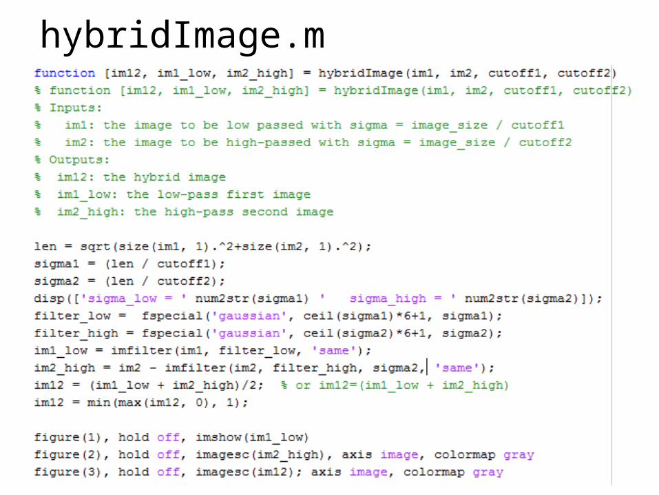
hybridImage.m

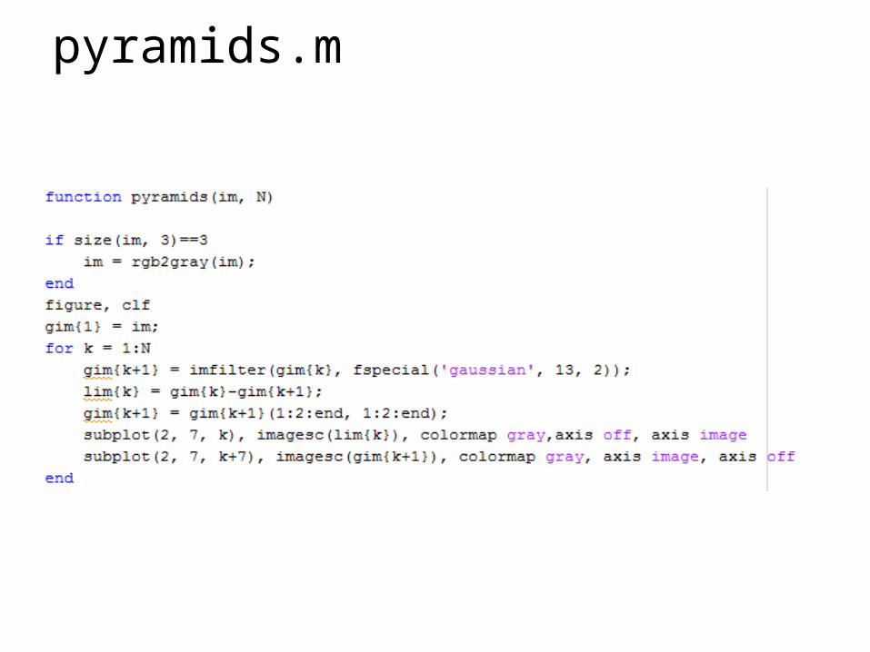
pyramids.m

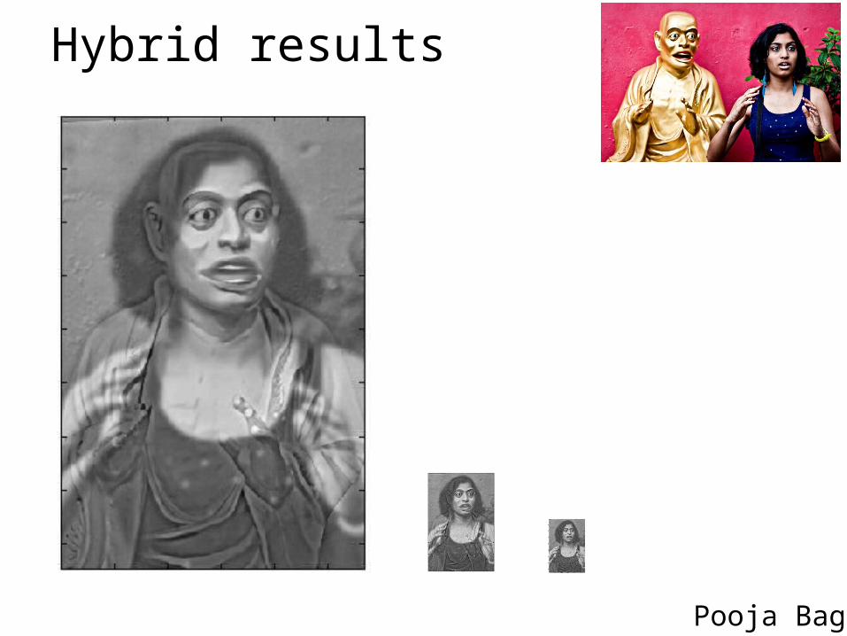
Hybrid results

Pooja Bag

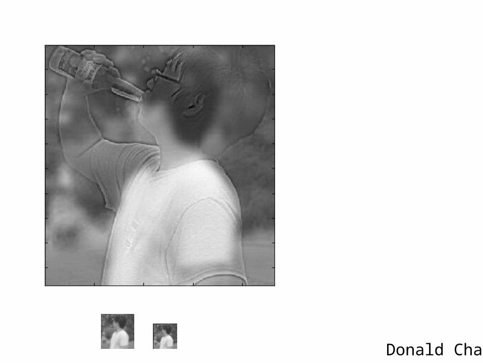
Donald Cha

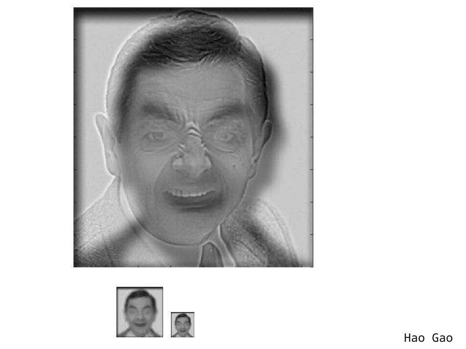
Hao Gao

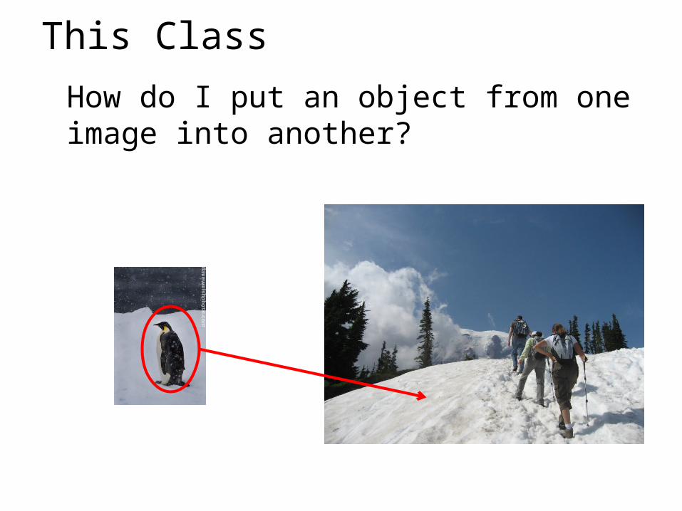
This Class

How do I put an object from one image into another?

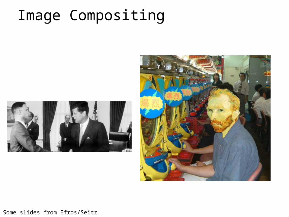
Image Compositing

Some slides from Efros/Seitz

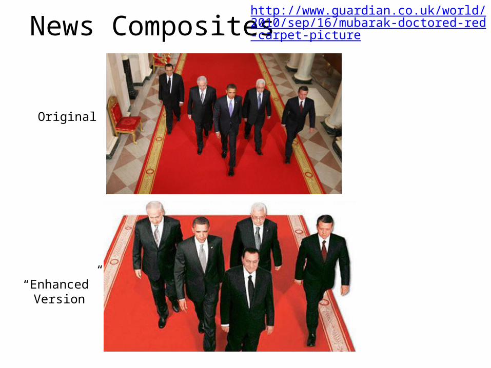
News Composites

Original

“Enhanced” Version

http://www.guardian.co.uk/world/2010/sep/16/mubarak-doctored-red-carpet-picture

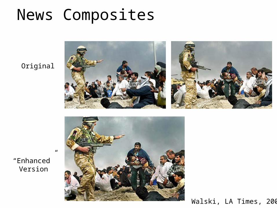
News Composites

Original

“Enhanced” Version

Walski, LA Times, 2003

Three methods

1. Cut and paste

2. Laplacian pyramid blending

3. Poisson blending

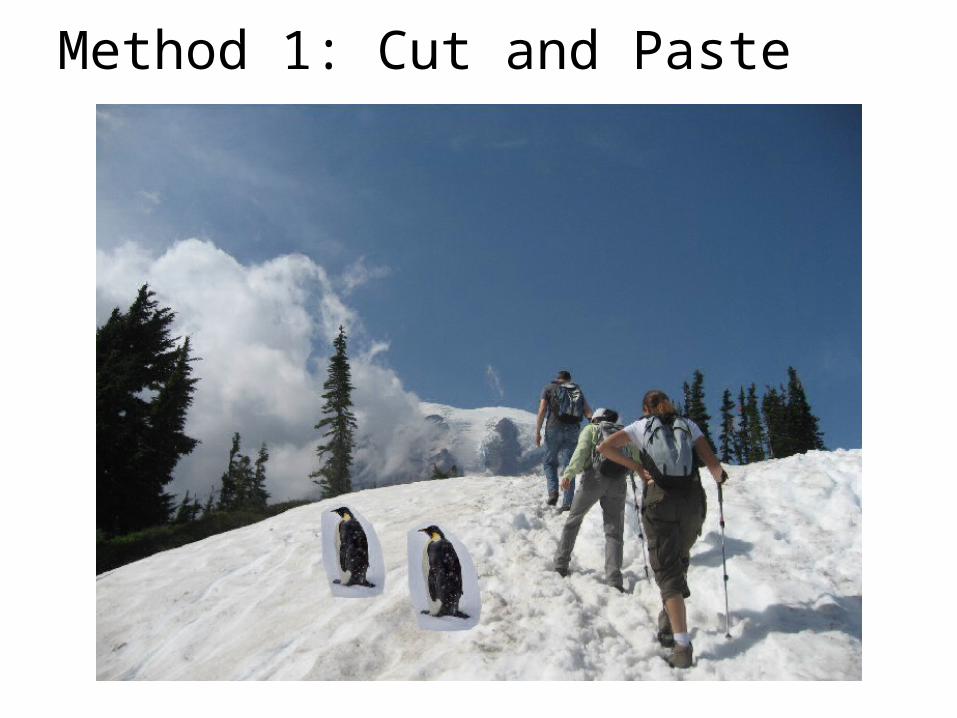
Method 1: Cut and Paste

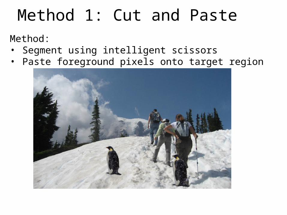
Method 1: Cut and PasteMethod:• Segment using intelligent scissors• Paste foreground pixels onto target region

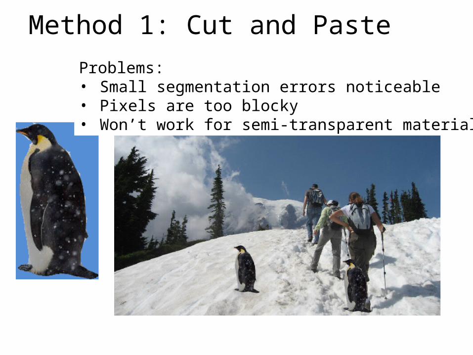
Method 1: Cut and PasteProblems:• Small segmentation errors noticeable• Pixels are too blocky• Won’t work for semi-transparent materials

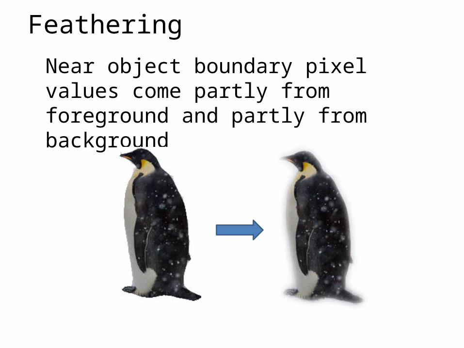
Feathering

Near object boundary pixel values come partly from foreground and partly from background

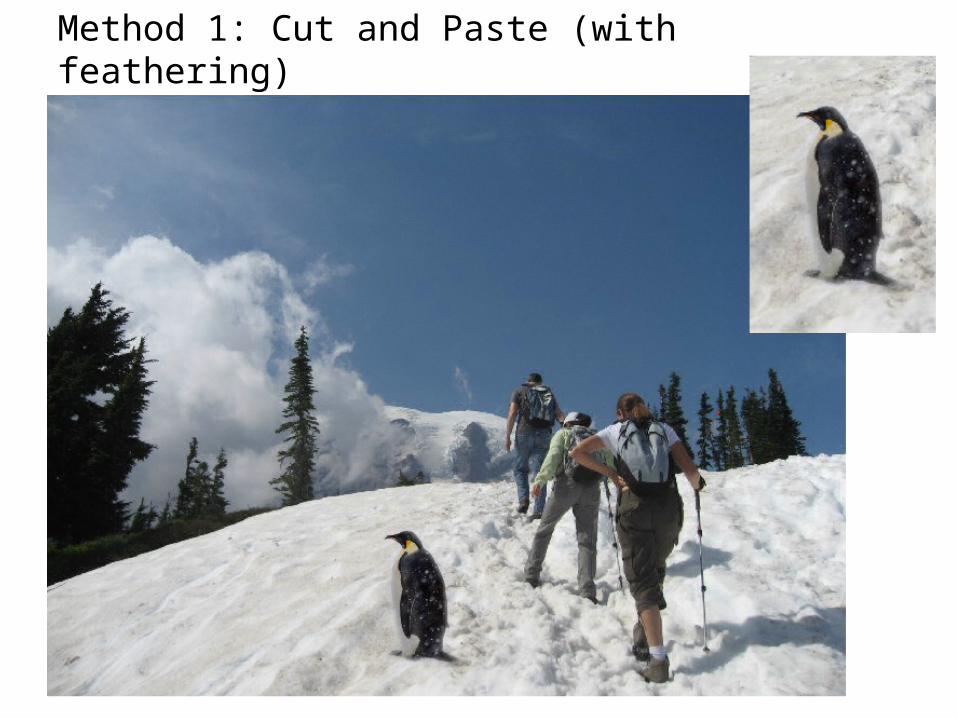
Method 1: Cut and Paste (with feathering)

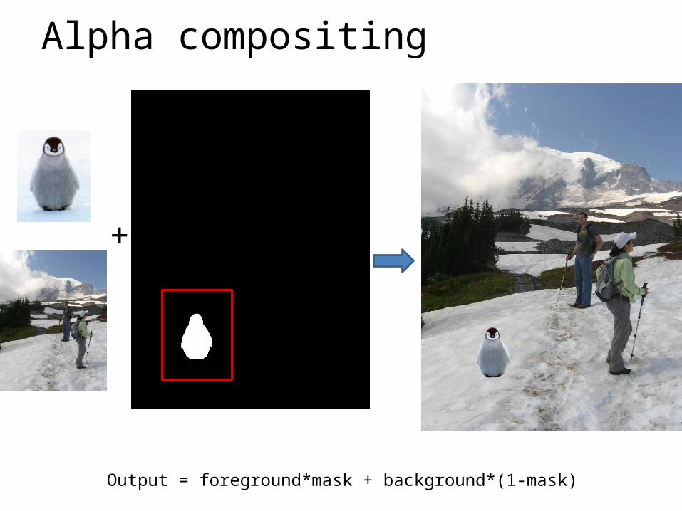
Alpha compositing

+

Output = foreground*mask + background*(1-mask)

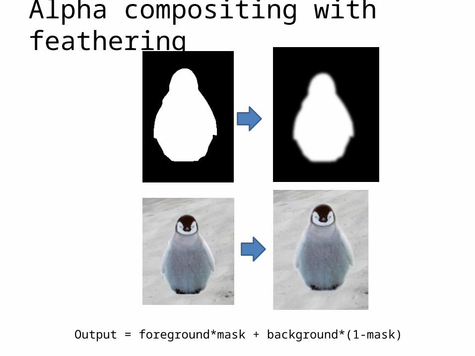
Alpha compositing with feathering

Output = foreground*mask + background*(1-mask)

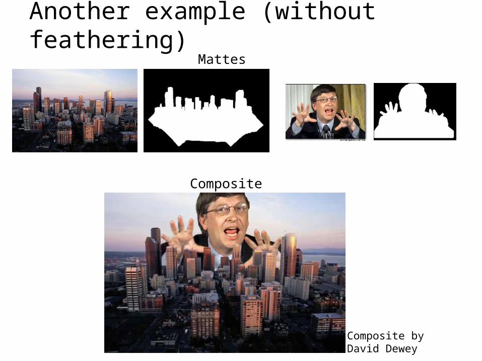
Another example (without feathering)Mattes

Composite by David Dewey

Composite

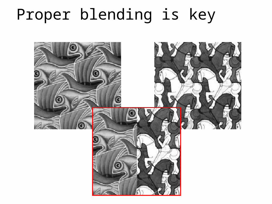
Proper blending is key

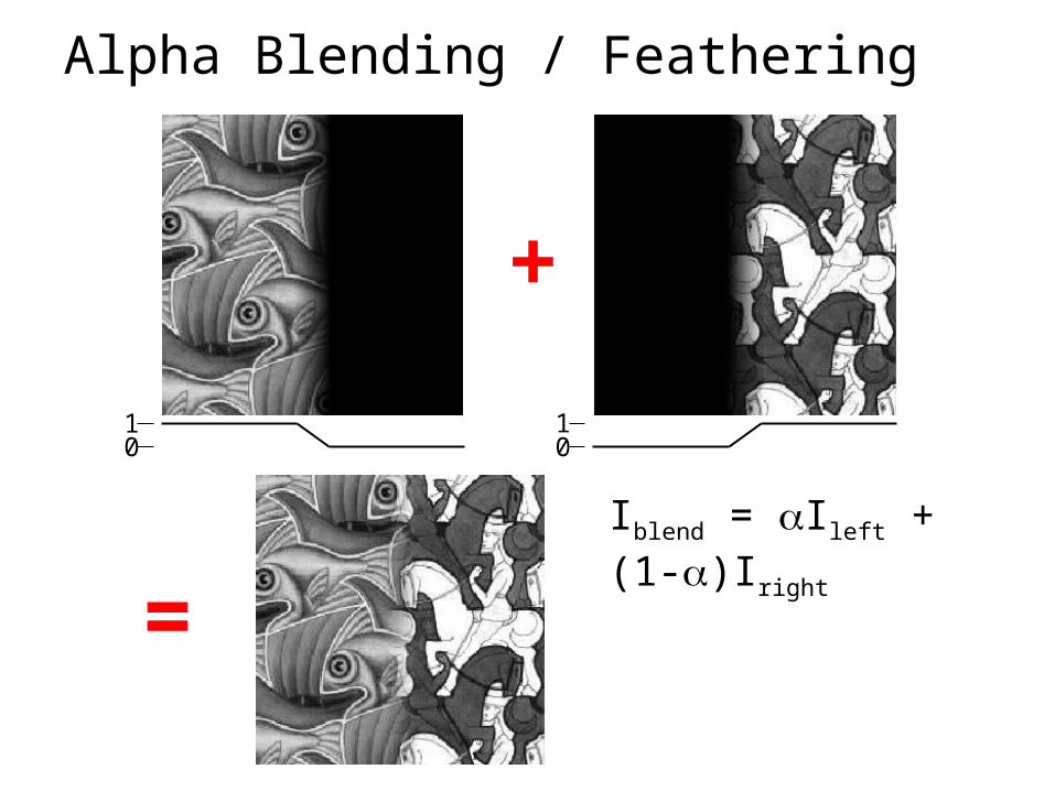
Alpha Blending / Feathering

01

01

+

=Iblend = aIleft + (1-a)Iright

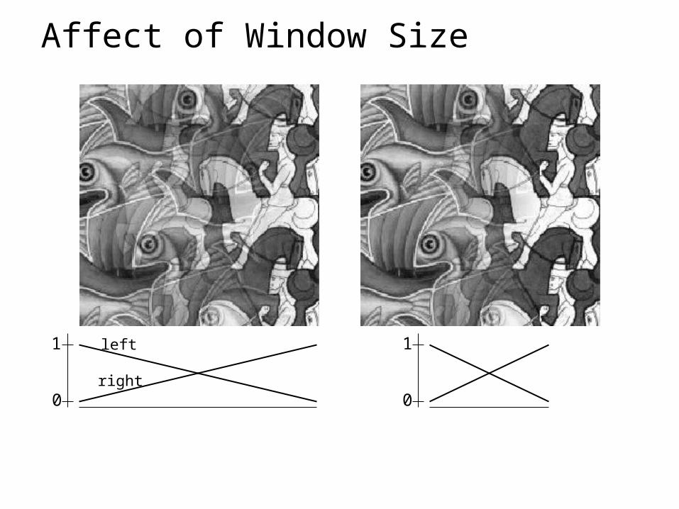
Affect of Window Size

0

1 left

right0

1

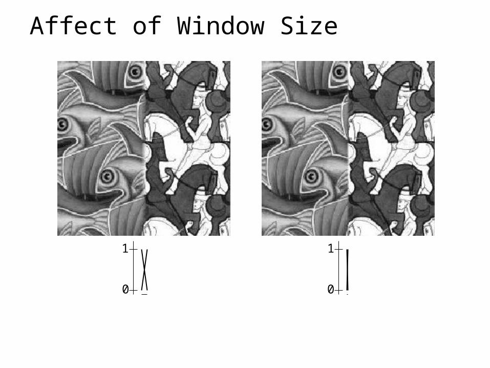
Affect of Window Size

0

1

0

1

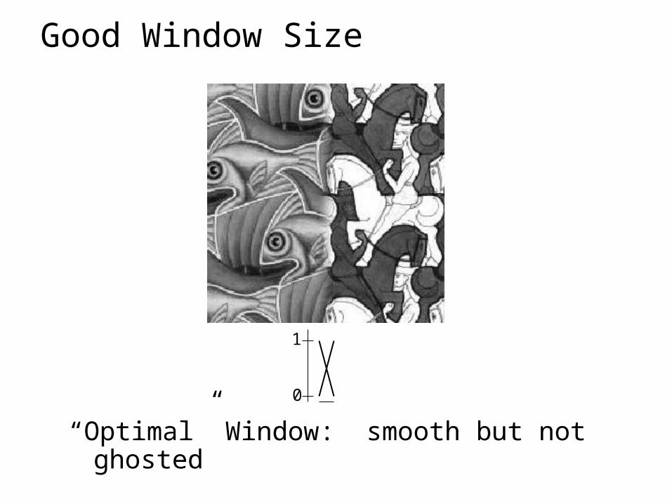
Good Window Size

0

1

“Optimal” Window: smooth but not ghosted

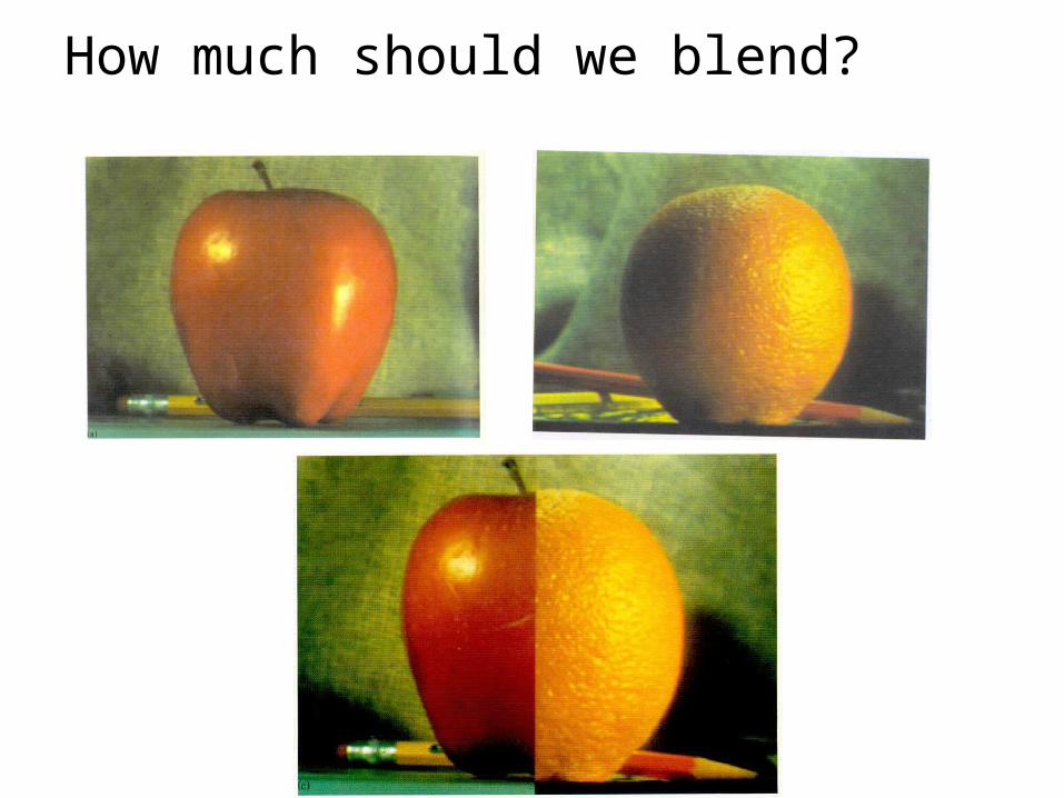
How much should we blend?

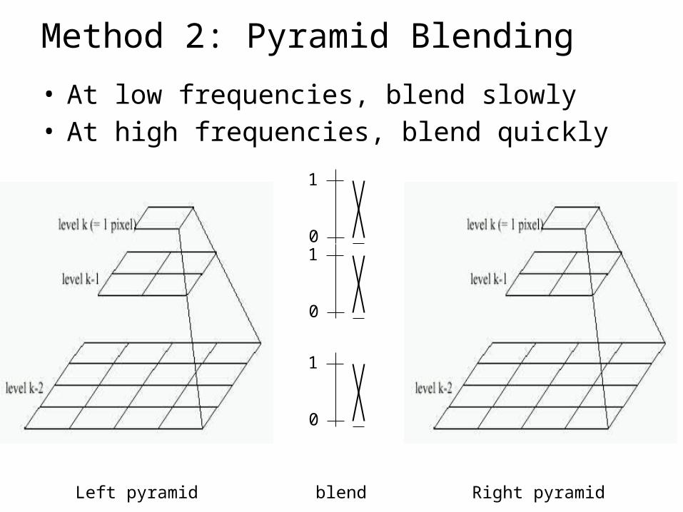
Method 2: Pyramid Blending

0

1

0

1

0

1

Left pyramid Right pyramidblend

• At low frequencies, blend slowly• At high frequencies, blend quickly

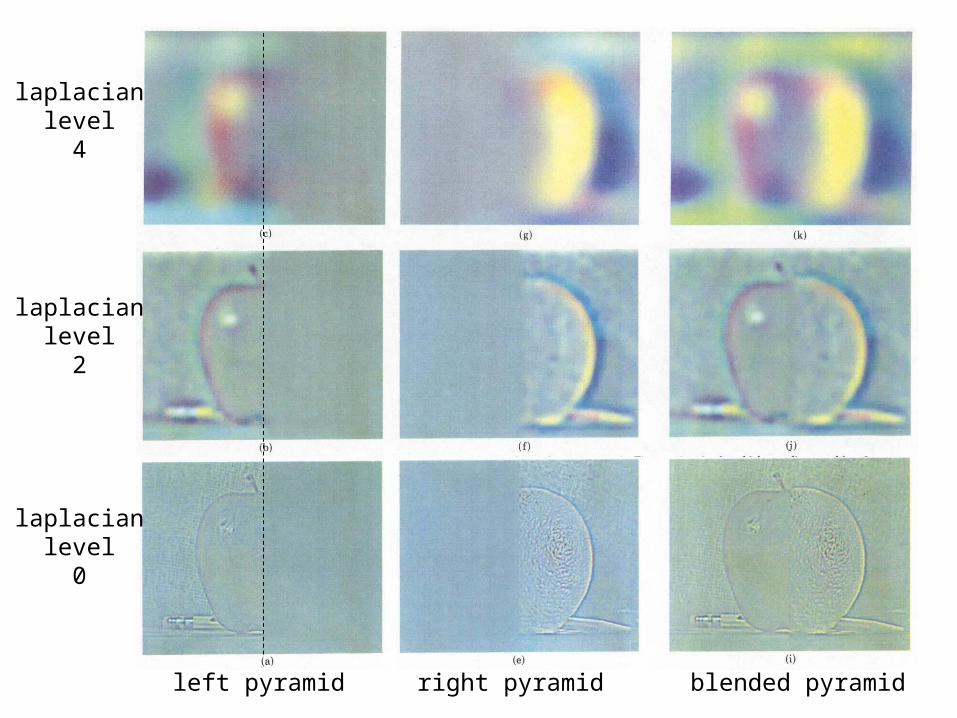
laplacianlevel

4

laplacianlevel

2

laplacianlevel

0

left pyramid right pyramid blended pyramid

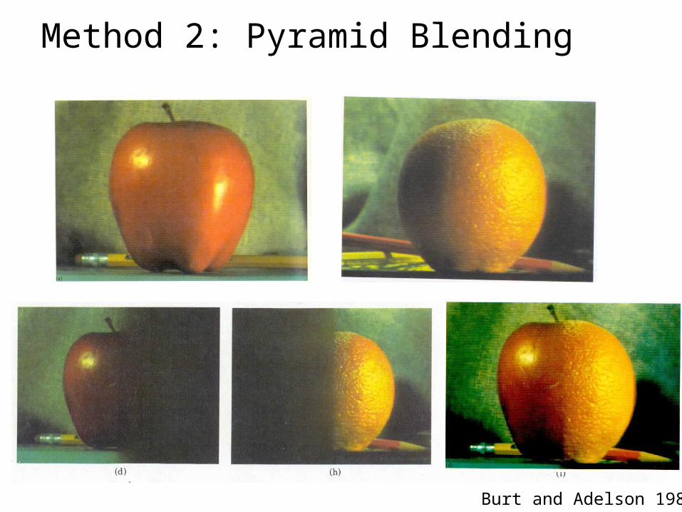
Method 2: Pyramid Blending

Burt and Adelson 1983

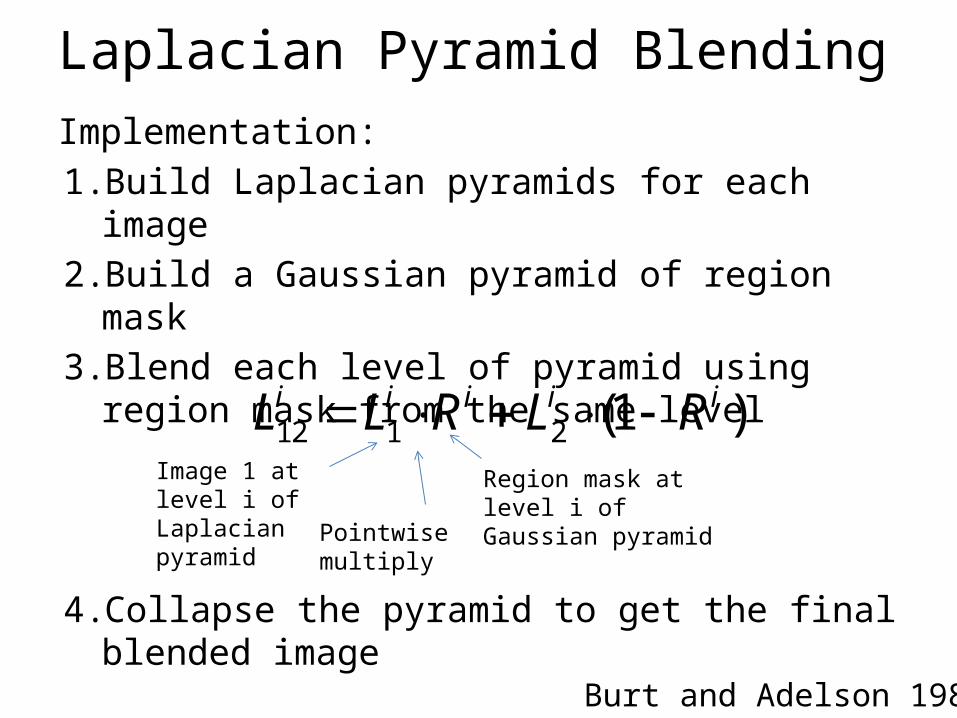
Laplacian Pyramid BlendingImplementation:1. Build Laplacian pyramids for each image2. Build a Gaussian pyramid of region mask3. Blend each level of pyramid using region mask from

the same level

4. Collapse the pyramid to get the final blended image

)1(2112iiiii RLRLL

Burt and Adelson 1983

Region mask at level i of Gaussian pyramid

Image 1 at level i of Laplacian pyramid

Pointwise multiply

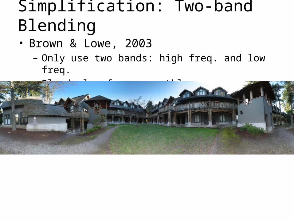
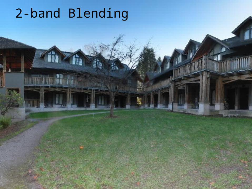
Simplification: Two-band Blending

• Brown & Lowe, 2003– Only use two bands: high freq. and low freq.– Blends low freq. smoothly– Blend high freq. with no smoothing: use binary alpha

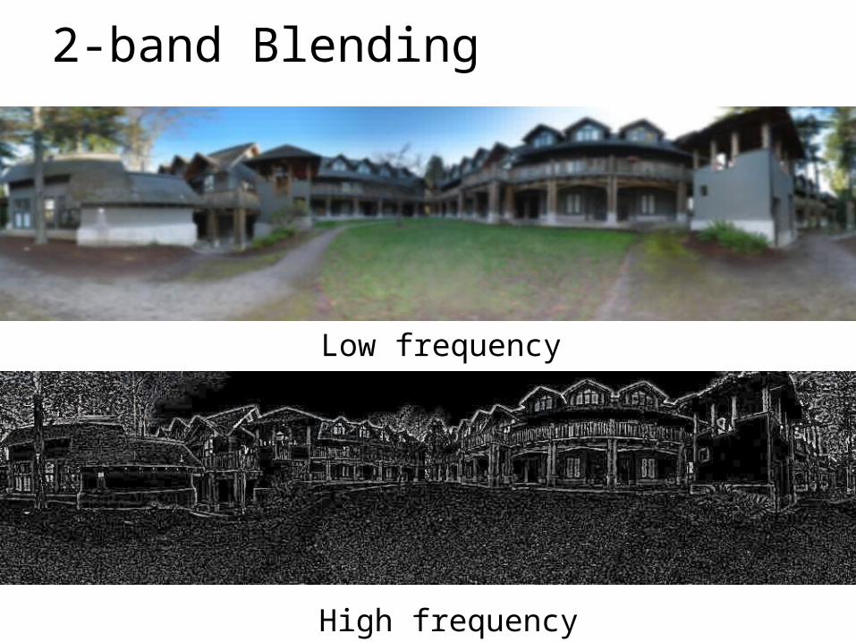
Low frequency

High frequency

2-band Blending

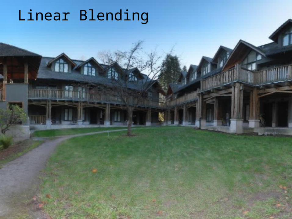
Linear Blending

2-band Blending

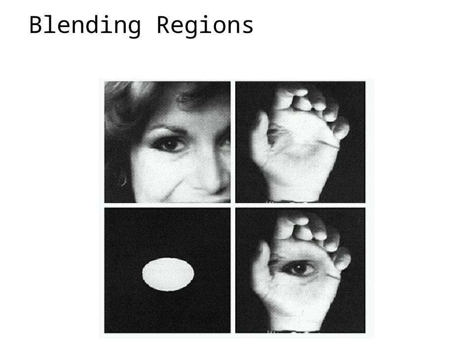
Blending Regions

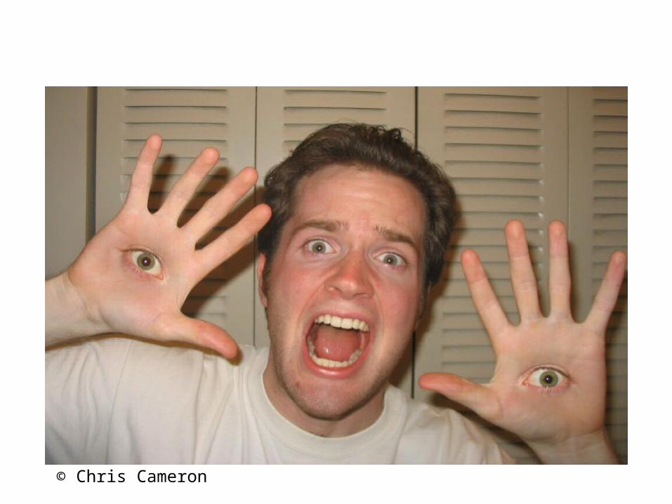
© Chris Cameron

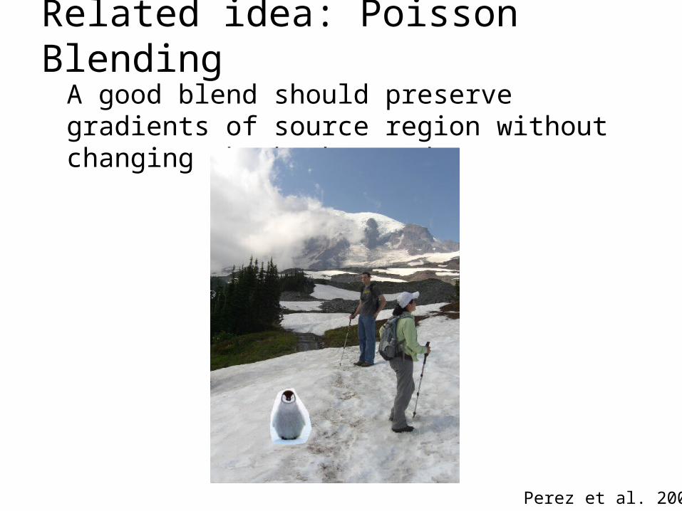
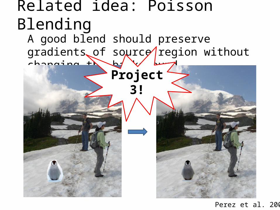
Related idea: Poisson BlendingA good blend should preserve gradients of source region without changing the background

Perez et al. 2003

Related idea: Poisson BlendingA good blend should preserve gradients of source region without changing the background

Perez et al. 2003

Project 3!

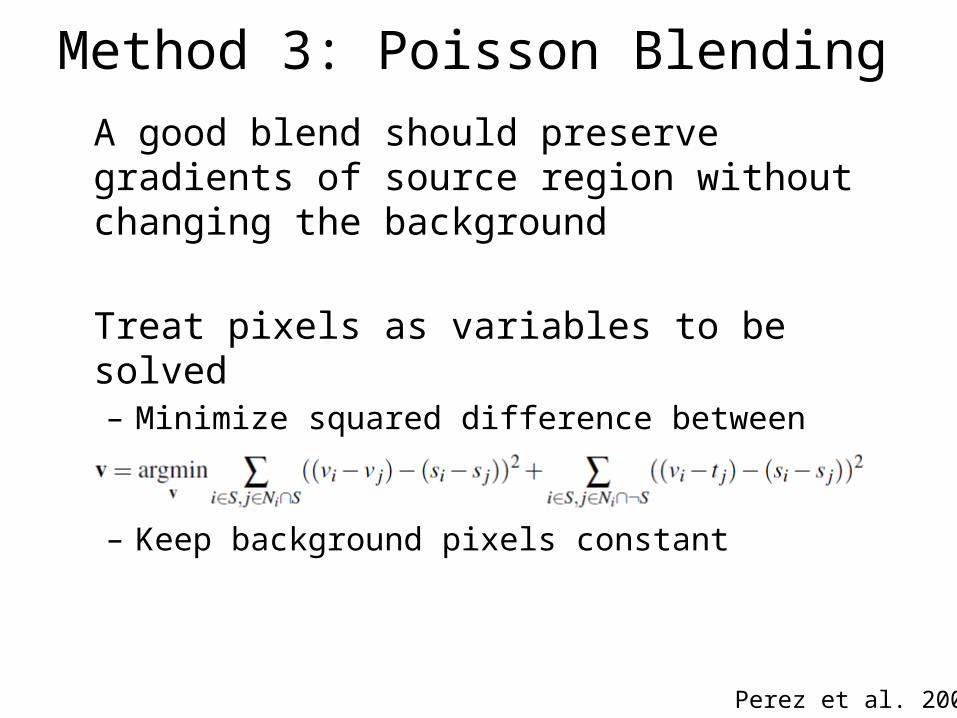
Method 3: Poisson BlendingA good blend should preserve gradients of source region without changing the background

Treat pixels as variables to be solved– Minimize squared difference between gradients of

foreground region and gradients of target region– Keep background pixels constant

Perez et al. 2003

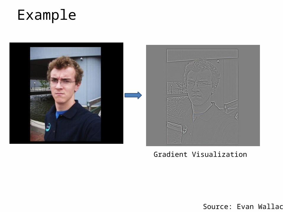
Example

Source: Evan Wallace

Gradient Visualization

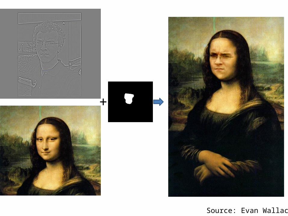
Source: Evan Wallace

+Specify object region

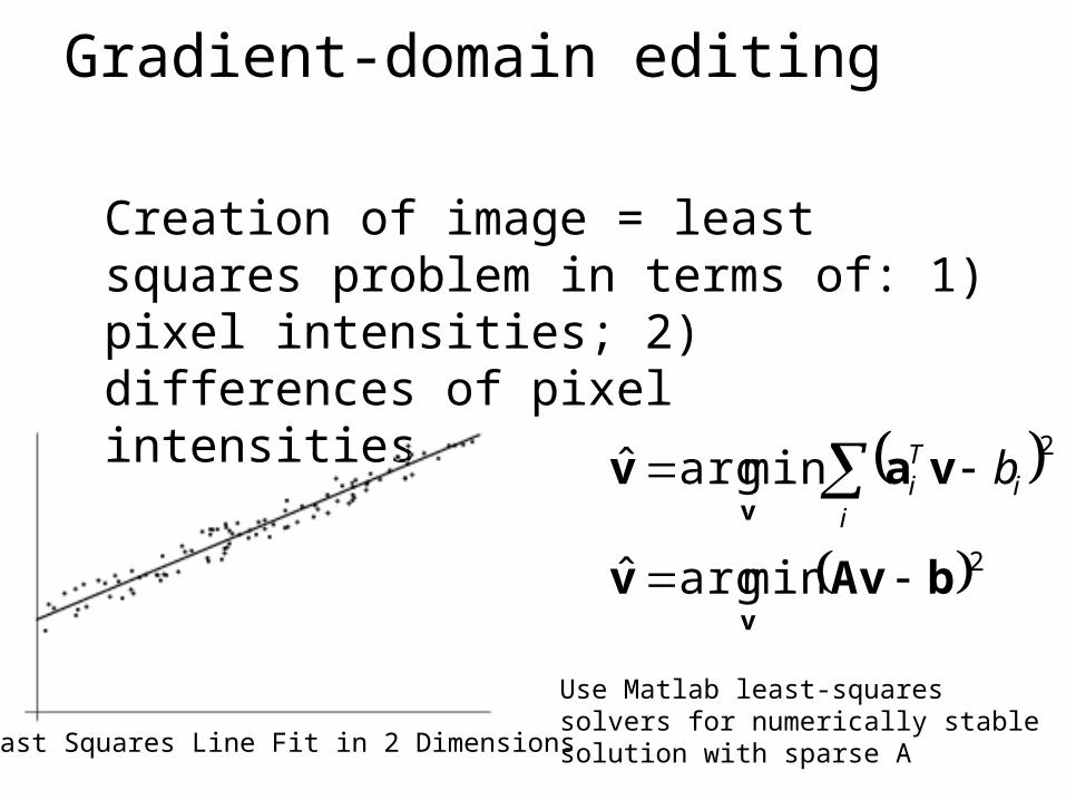
Gradient-domain editing

Creation of image = least squares problem in terms of: 1) pixel intensities; 2) differences of pixel intensities

Least Squares Line Fit in 2 Dimensions

2

2

minargˆ

minargˆ

bAvv

vav

v

v

i

iTi b

Use Matlab least-squares solvers for numerically stable solution with sparse A

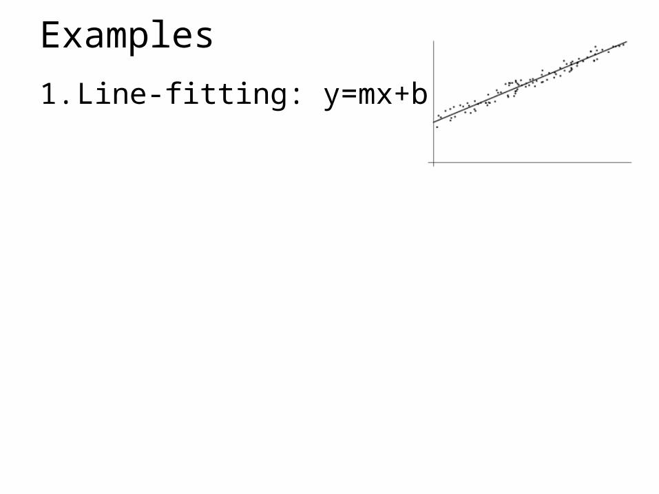
Examples

1. Line-fitting: y=mx+b

Examples

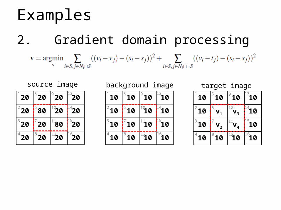
2. Gradient domain processing

20 20 20 20

20 80 20 20

20 20 80 20

20 20 20 20

1

2

3

4

5

6

7

8

9

10

11

12

13

14

15

16

10 10 10 10

10 10 10 10

10 10 10 10

10 10 10 10

1

2

3

4

5

6

7

8

9

10

11

12

13

14

15

16

source image background image target image

10 10 10 10

10 v1 v310

10 v2 v410

10 10 10 10

1

2

3

4

5

6

7

8

9

10

11

12

13

14

15

16

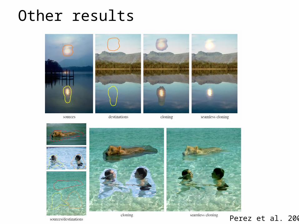
Other results

Perez et al. 2003

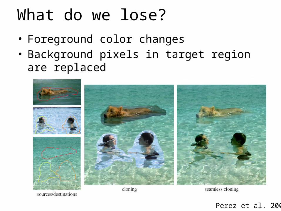
What do we lose?

Perez et al. 2003

• Foreground color changes• Background pixels in target region are replaced

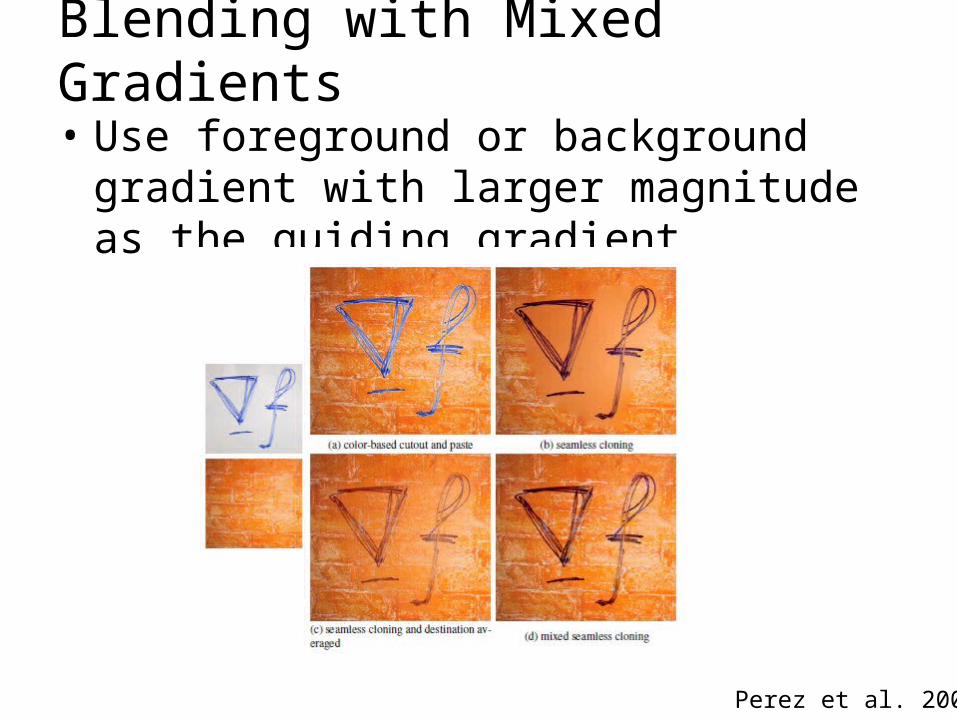
Blending with Mixed Gradients• Use foreground or background gradient with

larger magnitude as the guiding gradient

Perez et al. 2003

Project 3: Gradient Domain Editing

General concept: Solve for pixels of new image that satisfy constraints on the gradient and the intensity– Constraints can be from one image (for filtering)

or more (for blending)

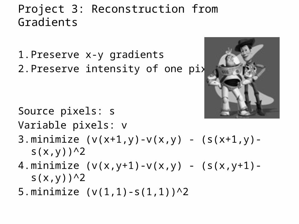
Project 3: Reconstruction from Gradients

1. Preserve x-y gradients2. Preserve intensity of one pixel

Source pixels: sVariable pixels: v3. minimize (v(x+1,y)-v(x,y) - (s(x+1,y)-s(x,y))^2 4. minimize (v(x,y+1)-v(x,y) - (s(x,y+1)-s(x,y))^2 5. minimize (v(1,1)-s(1,1))^2

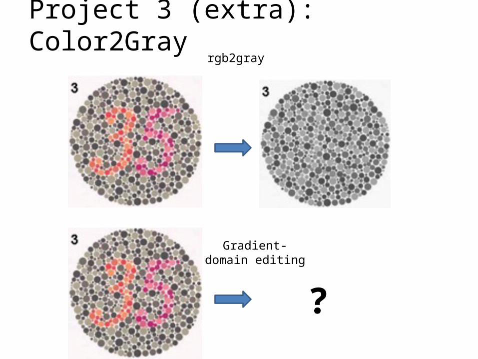
Project 3 (extra): Color2Grayrgb2gray

?

Gradient-domain editing

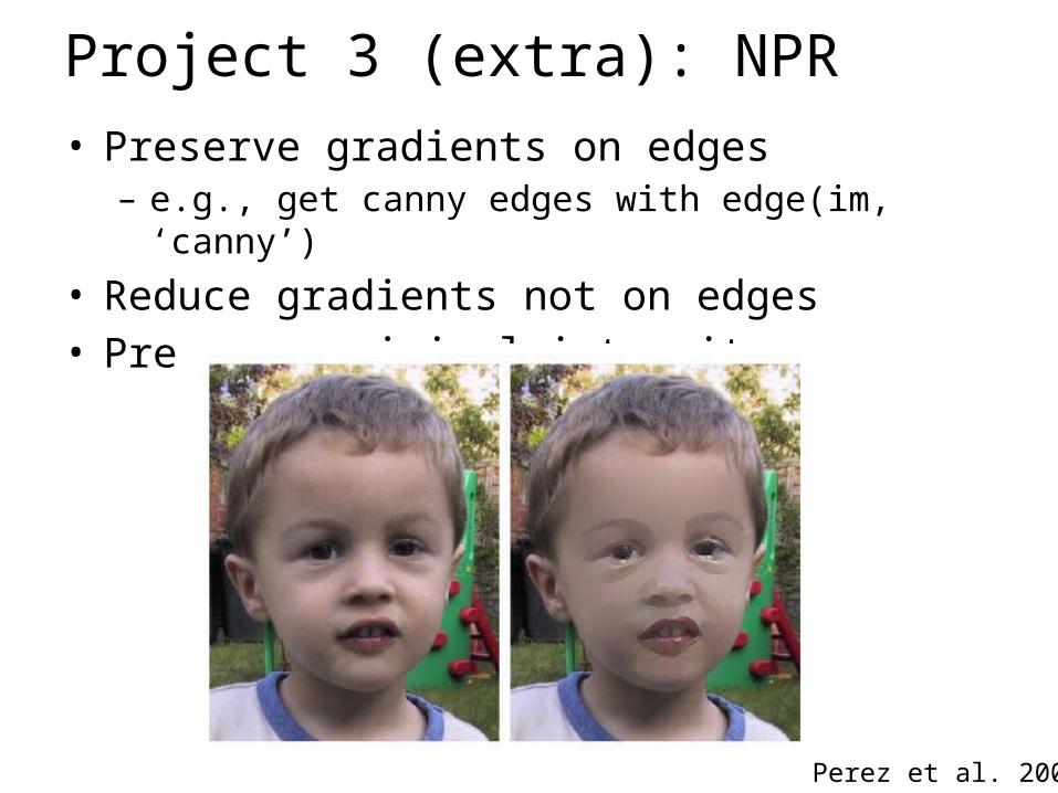
Project 3 (extra): NPR• Preserve gradients on edges

– e.g., get canny edges with edge(im, ‘canny’)

• Reduce gradients not on edges• Preserve original intensity

Perez et al. 2003

DVS Camera Links• Pencil balance

– https://www.youtube.com/watch?v=XVR5wEYkEGk

• Quad Copter• https://www.youtube.com/watch?v=LauQ6LWTkxM

• Tennis• https://www.youtube.com/watch?v=G1j2LLY5RIQ&t=27