block cave production scheduling optimization using mixed

Pourrahimian Y. et al. MOL Report Three © 2011 - ISBN: 978-1-55195-281-9 105-1

Block Cave Production Scheduling Optimization using Mixed Integer Linear Programming

Yashar Pourrahimian and Hooman Askari-Nasab Mining Optimization Laboratory (MOL) University of Alberta, Edmonton, Canada

Abstract

Planning of caving operations poses complexities in different areas such as safety, environment, ground control, and production scheduling. As the mining industry is faced with more marginal resources, it is becoming essential to generate production schedules which will provide optimal operating strategies while meeting practical, technical, and environmental constraints.

Production scheduling of any mining operation has an enormous effect on the economics of the venture. The scheduling problems are complex due to the nature and variety of the constraints acting upon the system. Relying only on manual planning methods or computer software based on heuristic algorithms will lead to mine schedules that are not the global optimal solution.

The objective of this paper is to develop a practical optimization framework for production scheduling of caving operations. A mixed integer linear programming (MILP) formulation is developed, implemented and verified in TOMLAB/CPLEX environment. The production scheduler aims at maximizing the net present value (NPV) of the mining operation while the mine planner has control over the development rate, vertical mining rate (production rate per drawpoint), lateral mining rate (rate of opening new drawpoints), dilution entry, mining capacity, maximum number of active drawpoints, cave draw strategies and advancement direction, and draw rate. The production scheduler defines the opening and closing time of each drawpoint, the draw rate from each drawpoint, the number of new drawpoints that need to be constructed, and the sequence of extraction from the drawpoints to support a given production target. The successful application of the model for production scheduling of a real mine data is also presented.

1. Introduction

Long-term mine production scheduling is one of the optimization problems. A production schedule must provide a mining sequence that takes into account the physical limitations of the mine and, to the extent possible, meets the demanded quantities of each raw ore type in each period throughout the mine life.

Underground mining is more complex in nature than surface mining (Kuchta et al., 2004). Underground mining is less flexible than surface mining due to the geotechnical, equipment, and space constraints (Topal, 2008).

A number of optimization techniques have been used in the past; many include significant simplifications or fail to produce acceptable results within the required timeframe. In spite of the difficulties associated with the application of mathematical programming to production scheduling in underground mines, authors have attempted to develop methodologies to optimize production schedules. Mathematical programming is a generic term for a variety of optimization algorithms developed to solve different mathematical formulations. All share the combination of variables,

Pourrahimian Y. et al. MOL Report Three © 2011 - ISBN: 978-1-55195-281-9 105-2 constraints, and an objective function. The algorithms used to solve the variables all treat the problem as a multidimensional solution space. It also reduces complexity and uncertainty to a level that is manageable, providing a quantifiable basis for mine design and planning.

Williams et al. (1972) planned sublevel stoping operations for an underground copper mine over one year using a linear programming approximation model. Jawed (1993) formulated a linear goal programming model for production planning in an underground room and pillar coal mine. Tang et al. (1993) integrated linear programming with simulation to address scheduling decisions, as did Winkler (1998). Trout (1995) used the MIP method to schedule the optimal extraction sequence for underground sublevel stoping. Ovanic (1998) used mixed integer programming of type two special ordered sets to identify a layout of optimal stopes. Carlyle et al. (2001) presented a model that maximized revenue from Stillwater's platinum and palladium mine. Topal et al. (2003) generated a long-term production scheduling MIP model for a sub-level caving operation and successfully applied it to Kiruna Mine. Sarin et al. (2005) scheduled a coal mining operation with the objective of net present value maximization. Ataee-Pour (2005) critically evaluated some optimization algorithms according to their capabilities, restrictions and application for use in underground mining. McIssac (2005) formulated the scheduling of underground mining of a narrow veined polymetallic deposit utilizing MIP.

Scheduling of underground mining operations is primarily characterized by discrete decisions to mine blocks of ore, along with complex sequencing relationships between blocks. Since linear programming (LP) models cannot capture the discrete decisions required for scheduling, MIPs are generally the appropriate mathematical programming approach to scheduling.The methods currently used to compute production schedule in block cave mines can be classified in two main categories: (a) heuristic methods and (b) exact optimization methods.

Heuristic methods are particularly used to rapidly come to a solution that is hoped to be close to the best possible answer, or optimal solution. These methods are used when there is no known method to find an optimal solution under the given constraints.

The original heuristic methods were the manual draw charts used at the beginning of block caving. These methods evolved through use at Henderson mine where a way to avoid early dilution entry was described by constraining the draw profile to an angle of draw of 45 degrees (Dewolf, 1981). Heslop et al. (1981) described a volumetric algorithm to simulate the mixing along the draw cone. Carew (1992) described the use of a commercial package called PC-BC to compute production schedules at Cassiar mine. Diering (2000) showed the principles behind the commercial tool PC-BC to compute production schedules, providing several case studies where different draw methods have been applied depending on the ore body geometry and rock mass behavior.

The application of operation research methods to the planning of block cave mines was first described by Riddle (1976). This development intended to compute mining reserves and define the economic extent of the footprint. The final algorithm did not reflect the operational constraints of block caving described above since it worked with the block model directly instead of defining the concept of draw cone as an individual entity of the optimization process.

The first attempt to use mathematical programming in block cave scheduling was made by Chanda (1990) who implemented an algorithm to write daily orders. This algorithm was developed to minimize the variance of the milling feed in a horizon of three days. Guest et al. (2000) made another application of mathematical programming in block cave long term scheduling. In this case, the objective function was explicitly defined to maximize draw control behavior. However, the author stated that the implicit objective was to optimize NPV. There are two problems with this approach. The first one is that maximizing tonnage or mining reserves will not necessarily lead to maximum NPV. The second problem is the fact that draw control is a planning constraint and not an objective function. The objective function in this case would be to maximize tonnage, minimize dilution or maximize mine life.

Pourrahimian Y. et al. MOL Report Three © 2011 - ISBN: 978-1-55195-281-9 105-3 Rubio (2002) developed a methodology that would enable mine planners to compute production schedules in block cave mining. He proposed new production process integration and formulated two main planning concepts as potential goals to optimize the long term planning process, thereby maximizing NPV and mine life.

Rahal et al. (2003) used a dual objective mixed integer linear programming algorithm to minimize the deviation between the actual state of extraction (height of draw) and a set of surfaces that tend towards a defined draw strategy. This algorithm assumes that the optimal draw strategy is known. Nevertheless, it is postulated that by minimizing the deviation to the draw target, the disturbances produced by uneven draw can be mitigated.

Diering (2004) presented a non-linear optimization method to minimize the deviation between a current draw profile and the target defined by the mine planner. He emphasized that this algorithm could also be used to link the short-term plan with the long-term plan. The long-term plan is represented by a set of surfaces that are used as a target to be achieved based on the current extraction profile when running the short-term plans. Rubio et al. (2004a) presented an integer programming algorithm and an iterative algorithm to optimize long-term schedules in block caving integrating the fluctuation of metal prices in time.

We critically reviewed the MILP formulations of the block cave production scheduling problem. We modeled the problem considering different possible. We divided the major decision variables into two categories, continuous variables representing the portion of a slice that is going to be extracted in each period and binary integer variables controlling the order of extraction of drawpoints and the number of active drawpoints in each period. We implemented the optimization formulation in TOMLAB/CPLEX (Holmstrom, 1989-2009) environment. A scheduling case study with real mine data was carried out over fifteen periods to verify the MILP model.

The next section of the paper covers the assumptions, problem definition, and the notations of variables. Section 3 presents mixed integer linear programming formulation of the problem, while section 4 presents the numerical modeling techniques. Section 5 presents an example, conclusions and future work followed by the list of references in the next section.

2. Assumptions, problem definition, and notation

We assume that a geological block model represents the orebody, which is a three-dimensional array of rectangular or cubical blocks used to model orebodies and other sub-surface structures.

The column of rock above each drawpoint, draw cone, is simulated and stored in a slice file. The draw cones, which are vertical, are created based on the block model and the total column is divided into slices which match the vertical spacing of the geological block model. Numerical data are used to represent each attribute of the orebody such as tonnage, densities, grade of elements, elevations, percentage of dilution, and economic data for each slice. Five basic drawpoint layouts which are being used at caving operations include continuous trough, herringbone, offset herringbone, Henderson or Z design, and the El Teniente or parallelogram (Brown, 2003). This research assumed that the physical layout of the production level is offset herringbone. There is the assumption of selective mining, meaning that based on the existing conditions either all the material in the draw cone or some part of it can be extracted.

Fig. 1 shows different steps from creation of the initial block model to creation of the slices. All stages before scheduling are done using GEMS and PCBC (GEMCOMSoftwareInternational, 2011). First of all, using GEMS a block model is created to provide a quantitative description of the rockmass including and surrounding the cave zone. Then drawpoint locations are defined and block model data is converted into drawpoint based data using PCBC. Afterwards, the slices are constructed for each drawpoint. These slices represent the draw column above each drawpoint before any extraction begins. The best height of draw (BHOD) for each draw cone is estimated.

Pourrahimian Y. et al. MOL Report Three © 2011 - ISBN: 978-1-55195-281-9 105-4 The BHOD is the height which produces the best economic value and it is usually not discounted with time. The number of possibilities for finding the optimal height is equal to the number of slices above each drawpoint. A simple comparison of the dollar value for each combination (slice 1, then slices 1,2, then slices 1,2,3) allows the best height to be found. This process or technique is shown schematically in Fig. 2. The relevant dollar value of each number in the horizontal axis is equal to the summation of dollar values of slices 1 to that number. The maximum value, in this case, is obtained for slice number 33. If the height of each slice is h (m), the best height of draw for this drawpoint is 33h (m).

Fig. 1. Flow chart from initial block model to draw column.

Fig. 2. Determination of the BHOD

After applying the BHOD, the final height of draw is obtained. Afterwards the production schedule of a block cave mine can be optimized using the MILP formulation. The problem is maximizing the net present value of the mining operation while the mine planner has control over the development rate, vertical mining rate (production rate per drawpoint), lateral mining rate (rate of opening new drawpoints), dilution entry, mining capacity, maximum number of active drawpoints, cave draw strategies and advancement direction, and draw rate. To solve the problem, four decision variables are employed, one continuous decision variable and three binary integer variables. Two of them are used in controlling slice level and two in controlling drawpoint level. The continuous decision variable indicates the portion of extraction from each slice in each period and three binary integer variables control the number of active drawpoints, precedence of extraction between slices and drawpoints, the opening and closing time of each drawpoint, the draw rate from each drawpoint, and the number of new drawpoints that need to be constructed in each period. This

Block model Draw point locations Draw column

0.1

0.2 0.35

0.4

1.1 1.4

0.9 1.0

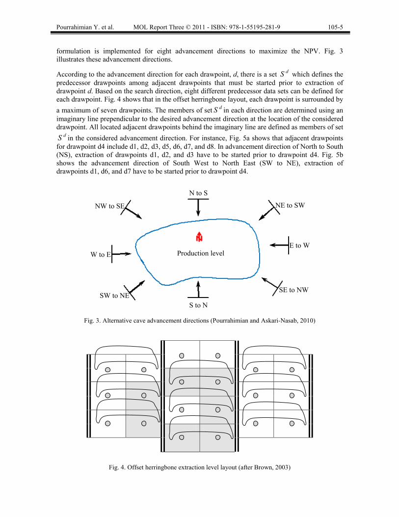
Pourrahimian Y. et al. MOL Report Three © 2011 - ISBN: 978-1-55195-281-9 105-5 formulation is implemented for eight advancement directions to maximize the NPV. Fig. 3 illustrates these advancement directions.

According to the advancement direction for each drawpoint, d, there is a set dS which defines the predecessor drawpoints among adjacent drawpoints that must be started prior to extraction of drawpoint d. Based on the search direction, eight different predecessor data sets can be defined for each drawpoint. Fig. 4 shows that in the offset herringbone layout, each drawpoint is surrounded by a maximum of seven drawpoints. The members of set dS in each direction are determined using an imaginary line prependicular to the desired advancement direction at the location of the considered drawpoint. All located adjacent drawpoints behind the imaginary line are defined as members of set

dS in the considered advancement direction. For instance, Fig. 5a shows that adjacent drawpoints for drawpoint d4 include d1, d2, d3, d5, d6, d7, and d8. In advancement direction of North to South (NS), extraction of drawpoints d1, d2, and d3 have to be started prior to drawpoint d4. Fig. 5b shows the advancement direction of South West to North East (SW to NE), extraction of drawpoints d1, d6, and d7 have to be started prior to drawpoint d4.

Fig. 3. Alternative cave advancement directions (Pourrahimian and Askari-Nasab, 2010)

Fig. 4. Offset herringbone extraction level layout (after Brown, 2003)

Production level

N to S

S to N

W to E E to W

SE to NW

NW to SE

SW to NE

NE to SW


(b)

Fig. 5. Determination method of members for set dS in different directions.

2.1. Notation

The notation of decision variables, parameters, sets, and constraints are as follows:

2.1.1. Sets

dS For each drawpoint, d, there is a set dS defining the predecessor drawpoints that must be started prior to extraction of drawpoint d.

d sS For each drawpoint, d, there is a set d sS defining the slices in draw cone associated with drawpoint d.

sS For each slice, s, there is a set sS defining the predecessor slice that must be extracted prior to extraction of slice s.

d l sS For each drawpoint, d, there is a set d l sS defining the lowest slice within the draw cone associated with drawpoint d.

2.1.2. Indices

{1,...., }t T∈ Index for scheduling periods.

{1,..., }d D∈ Index for drawpoints.

{1,..., }s S∈ Index for slices.

{1,..., }e E∈ Index for elements of interest in each slice.

m Index for a slice belonging to one of the sets sS or d l sS

j Index for a drawpoint belonging to one of the sets dS or d sS

2.1.3. Parameters

sSEV Economic value of slice s.

i The discount rate.

dN Number of drawpoints.

dNs Number of slices within the draw cone associated with drawpoint d.

dDC Development and construction cost of drawpoint d.

d sSC Development and construction cost of slice s in the draw cone associated with drawpoint d.

atN Maximum number of active drawpoints in period t.

ntN Upper limit of number of new drawpoints in period t.

(a)

d1

d2 d3

d4 d5

d6

d7 d8

d1

d2 d3

d4 d5

d6

d7 d8


ntN Lower limit of number of new drawpoints in period t.

sO Total tonnage of ore in slice s.

sW Total tonnage of waste in slice s.

s sO W+ Total tonnage of material in slice s.

dTD Total tonnage of material in draw cone associated with drawpoint d.

esG Average grade of element e in ore portion of slice s.

etG Upper limit of acceptable average head grade of element e in period t.

etG Lower limit of acceptable average head grade of element e in period t.

tM Upper limit of mining capacity in period t.

tM Lower limit of mining capacity in period t.

d tDR Draw rate of drawpoint d in period t.

d tDR Minimum possible draw rate of drawpoint d in period t.

d tDR Maximum possible draw rate of drawpoint d in period t.

dγ Density of material in drawpoint d.

2.1.4. Decision variables

[0,1]s tX ∈ Continuous variable, representing the portion of slice s to be extracted in period t.

{0,1}d tE ∈ Binary integer variable controlling the starting period of drawpoints and the precedence of extraction of drawpoints. d tE is equal to one if extraction of drawpoint d has started by or in period t, otherwise it is zero.

{0,1}d tC ∈ Binary integer variable controlling the closing period of drawpoints. d tC is equal to one if extraction of drawpoint d has finished by or in period t, otherwise it is zero.

{0,1}s tB ∈ Binary integer variable controlling the precedence of extraction of slices. It is equal to one if extraction of slice s has started by or in period t, otherwise it is zero.

3. Mathematical model

A mixed integer linear programming (MILP) problem contains both integer and continuous variables and there are no quadratic terms in the objective function.

3.1. Objective function

The objective function of the MILP formulation is to maximize the net present value of the mining operation. The profit from mining a drawpoint depends on the value of the slices and the costs incurred in mining.

The objective function, Eq.(1), is composed of the slice economic value (SEV), discount rate, slice cost, and a continuous decision variable that indicates the portion of a slice which is extracted in each period. The most profitable slices will be chosen to be part of the production call in order to optimize the NPV.

Pourrahimian Y. et al. MOL Report Three © 2011 - ISBN: 978-1-55195-281-9 105-8 In Eq.(1), construction cost of drawpoint d is divided among the slices in the draw cone associated with drawpoint d. For example, if there are 15 slices in the draw cone associated with drawpoint number 20 and drawpoint development and construction cost of this drawpoint is $ DC20

, the cost of each slice within the relevant draw cone is given by Eq.(2).

( )1 1

Maximize1

T Ss

s sttt s

SEV SC Xi= =

− × +

∑∑ (1)

202020

$15

ss

DCSC s S= ∈ (2)

3.2. Constraints

3.2.1. Mining capacity

This constraint forces mining system to achieve desired mining capacity. It is applied using inequalities in Eq.(3), which ensures that the total tonnage of material extracted from drawpoints in each period is within the acceptable range that allows flexibility for potential operational variations.

{ }1

( ) 1,...,S

t s s s t ts

M O W X M t T=

≤ + × ≤ ∀ ∈∑ (3)

3.2.2. Grade blending

This constraint forces the mining system to achieve the desired grade. The average grade of the element of interest has to be greater than or equal to a certain value, etG , and less than or equal to

a certain value, etG , for each period t. It is applied using inequalities in Eq.(4), which ensure that the average grade of production is within the desired range in each period.

( )

( ){ } { }1

1

1,..., , 1,...,

S

es s s s ts

et etS

s s s ts

G O W XG G t T e E

O W X

=

=

× + ×≤ ≤ ∀ ∈ ∈

+ ×

∑

∑ (4)

3.2.3. Maximum number of active drawpoints and continuous extraction from draw cone

During the mine life, each drawpoint can be in three different situations: open, active, and close. Fig. 6 illustrates how the situations change. In each period, we need to know the number of active drawpoints because this number must not exceed the allowable number. This constraint controls the maximum number of active drawpoints at any given period of the schedule.

As an example, Fig. 7 shows that the draw cone associated with drawpoint d contains four slices. The starting period of extraction of drawpoint d can be controlled by the lowest slice. This means, extraction of drawpoint d is started by extraction of the relevant lowest slice. When extraction of the last portion of a slice is finished in period t, extraction of the above slice can be started in the period t or t+1. In other words, extraction of a slice can be started if the below slice is totally extracted. If extraction of a slice is not started after finishing the extraction of the below slice in period t or t+1, the relevant drawpoint must be closed. Fig. 8 shows values of variables when extraction of a slice is finished. The mentioned concept is applied using inequalities in Eqs.(5), (6), (7), and (8). Eq.(7) ensures that when drawpoint d is open, at least a portion of one of the slices within the draw cone associated with drawpoint d is extracted otherwise the drawpoint must be closed. This means extraction must be continuous otherwise the drawpoint will be closed. Parameter L in Eq.(7) must be a big enough number. Eqs.(6) and (8) ensure that when variables


Lowest Slice

Drawpoint d

d tE and d tC change to one, they remain one until the end of the mine life. This helps us to recognize the periods when the drawpoint is active. Fig. 9 shows the relationship between opening time, closing time, and active time. Eq. (9) controls the maximum number of active drawpoints in each period. atN should be given as an input to the algorithm.

Fig. 6. Changes of drawpoint situation during the mine life

Fig. 7. Extraction time of the lowest slice is equivalent to drawpoint starting period.

Fig. 8. Value of variables when extraction of a slice is finished.

{ }0 1,..., , {1,..., }, dlss t d tX E t T d D s S− ≤ ∀ ∈ ∈ ∈ (5)

{ }( 1) 0 1,..., , {1,..., }d t d tE E t T d D+− ≤ ∀ ∈ ∈ (6)

{ }1,..., , {1,..., }, d sd t d t mtE C L X t T d D m S− ≤ × ∀ ∈ ∈ ∈∑ (7)

{ }( 1) 0 1,..., , {1,..., }d t d tC C t T d D+− ≤ ∀ ∈ ∈ (8)

Time

Mine life

Open Close

Active

Before opening After closing

Slice

1, 1, 1

ts d s

g i g ti

g S and S X B=

∈ = =∑

Extraction Finished Slice g

1d tE =

Slices, in period t ( ),s t s tX B and in the period t+1 ( ), 1 , 1,s t s tX B+ +


Mine life

0d tE = 1d tE =

0d tC = 1d tC =

Drawpoint life ( Drawpoint is active)

1d t d tE C− =

0d t d tE C− = 0d t d tE C− =

→ Extraction has been finished in period t if 1

1t

ss i

iX s S′

=

′= ∈∑

Slice s

Slice s′

{ }1

( ) 1,...,D

d t d t atd

E C N t T=

− ≤ ∀ ∈∑ (9)

3.2.4. Precedence

• Drawpoints

These constraints control the extraction precedence of drawpoints. Eq. (10) ensures that all drawpoints belonging to the relevant set, dS , have been started prior to extraction of drawpoint d. This set is defined based on the selected mining advancement direction. This set can be empty, which means the considered drawpoint can be extracted in any time period in the schedule. Eq.(10) ensures that only the set of immediate predecessor drawpoints need to be started prior to starting the drawpoint under consideration.

{ }0 {1,..., }, 1,..., , dj t d tE E d D t T j S− ≤ ∀ ∈ ∈ ∈ (10)

• Slices

Extraction of slice, s, can be started if the slice below it has been extracted totally. Fig. 10 shows that for each slice except the lowest, there is a set sS defining the predecessor slice that must be extracted prior to extraction of slice s. The extraction precedence of slice within each draw cone is controlled by Eqs.(11), (12) and (13). Eqs. (11) and (12) ensure that extraction of slice belonging to the relevant set,

sS , has been finished prior to extraction of slice s. Eq.(14) ensures that slice s is extracted when the relevant drawpoint is active.

Fig. 10. Sequence of extraction between slices

Fig. 9. Drawpoint activity duration based on opening and closing periods


{ }1

0 {1,..., }, 1,..., ,t

ss t mi

i

B X s S t T m S=

− ≤ ∀ ∈ ∈ ∈∑ (11)

{ }1

0 {1,..., }, 1,...,t

s i s ti

X B s S t T=

− ≤ ∀ ∈ ∈∑ (12)

{ }( 1) 0 {1,..., }, 1,...,s t s tB B s S t T+− ≤ ∀ ∈ ∈ (13)

{ }{1,..., }, 1,..., ,mt d sd t d t

d

XE C d D t T m S

Ns≤ − ∀ ∈ ∈ ∈∑ (14)

3.2.5. Number of new drawpoints (Development rate)

This constraint defines the maximum feasible number of drawpoints to be opened at any given time within the scheduled horizon. This constraint is usually based on the footprint geometry, the geotechnical behavior of the rock mass and the existing infrastructure of the mine, which will typically define available mining faces.

The drawpoint opening is controlled by the variable d tE , which takes a value of one from the opening period to end of the mine life. From period two to the end of the mine life, the difference

between the summation of opened drawpoints until and including period t,1

{2,..., }D

d td

E t T=

∈∑ , and

the summation of opened drawpoints until and including previous period t-1,

( 1)1

{2,..., }D

d td

E t T−=

∈∑ , indicates the number of new drawpoints. Eq.(15) ensures that the number

of new drawpoints which are opening in each period except period one is within the acceptable range. Eq. (16) ensures that in period one the number of new drawpoints is equal to the number of active drawpoints.

( 1)1 1

{2,..., }D D

nt d t d t ntd d

N E E N t T−= =

≤ − ≤ ∀ ∈∑ ∑ (15)

1 11

D

d ad

E N=

≤∑ (16)

3.2.6. Reserves

Eq.(17) ensures that there is selective mining for the slices, and thereby based on the existing conditions either all the material in the draw cone or some part of that can be extracted.

{ }1

1 1,...,T

stt

X s S=

≤ ∀ ∈∑ (17)

3.2.7. Draw rate

This constraint controls the maximum and minimum rate of draw and is a function of fragmentation and capability. This rate should be fast enough to avoid compaction and slow enough to avoid air gaps. The maximum limit to the draw rate is usually determined by the fragmentation process since time is required to achieve good fragmentation. However, sometimes, the maximum rate may be determined by the LHD productivity. Inequalities in Eq. (18) ensure that the draw rate from each drawpoint is within the desired range in each period.


( ) ( ) { }. . {1,..., }, 1,..., , d sd t d t d t m m mt d tE C DR O W X DR d D t T m S− ≤ + ≤ ∀ ∈ ∈ ∈∑ (18)

4. Numerical modeling

To solve linear programming problems in which the variables of the objective function are continuous in the mathematical sense, with no gaps between real values, ILOG CPLEX implements optimizers based on simplex algorithms (Winston, 1995) (both primal and dual simplex) as well as primal-dual logarithmic barrier algorithms.

The branch‐and‐cut method is an efficient way for solving combinatorial optimization problems that are formulated as mixed integer linear programming problems. It is an exact algorithm which combines cutting plane and the branch‐and‐bound algorithms. It works by solving a sequence of linear programming relaxations of the IP problem. The cutting plane improves the relaxation of the problem to a closer approximation (Horst and Hoang, 1996).

In this study we used

Table 1

TOMLAB/CPLEX version 12.1.0 (Holmström, 1989-2009) as the MILP solver. TOMLAB/CPLEX efficiently integrates the solver package CPLEX (ILOGInc, 2007) with a MATLAB environment(MathWorksInc, 2007).

represents the required number of decision variables for the proposed MILP formulation as a function of the number of drawpoints, dN , number of slices, sN , and number of scheduling periods, T. Thus, the number of continuous and binary decision variables for each problem are ( )sN T× and ( )2 d sT N N × + , respectively.

Table 1. Number of decision variables in the presented formulation Variable Type Relevant level Number of

variables s tX continuous Slice sN T×

s tB binary Slice sN T×

d tE binary Drawpoint dN T×

d tC binary Drawpoint dN T×

5. Illustrative example

The presented model has been implemented and tested in TOMLAB/CPLEX environment. It was verified based on a real data set containing 20 drawpoints. There were 607 slices in the primary slice data file which was reduced to 324 after calculating the BHOD. Fig. 11 illustrates tonnage and grade distribution of the 324 slices. The grade of copper varies between 0.7and 1.5 percent and the majority of slices are more than 6000 tonnes. The total tonnage of material within drawpoints is almost 2.08 Mt. Fig. 12 shows a plan view of the drawpoints and tunnels based on relevant coordinates. Fig. 13 illustrates a 3D view of draw columns. As can be seen, southern draw columns are taller than northern ones.


Fig. 11. Tonnage and grade distribution of slices

Fig. 12. Plan view of drawpoints and tunnels

6. Results and discussion

The presented MILP formulation was implemented for all mining advancement directions to find the optimum production schedule. Table 2 shows CPU time and size of the problem to test the MILP model for 20 drawpoints over 15 periods of extraction along the different advancement directions. The same scheduling parameters were used as input to solve the problem in the different advancement directions (see Table 3)

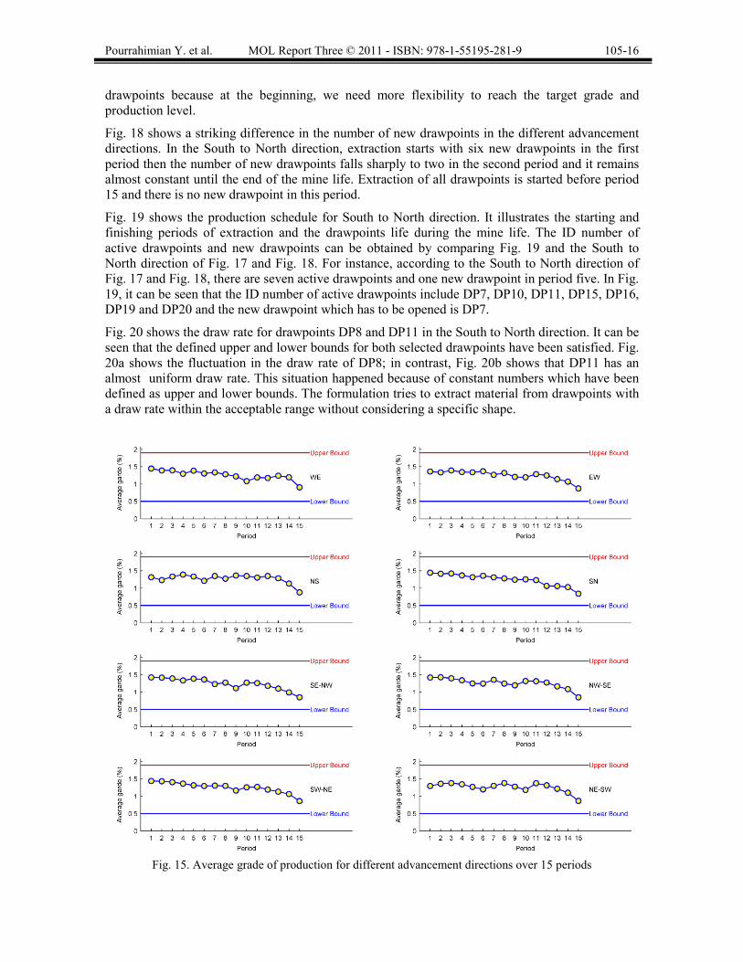
Table 3 shows scheduling parameters and obtained results for each advancement direction. Fig. 14 shows that difference between the highest and the lowest NPVs is more than five percent. The maximum NPV is obtained in the South to North direction. Fig. 15 to Fig. 22 show that all assumed constraints have been satisfied. Fig. 15 illustrates average grade of production for each period along the different advancement directions.

Cu grade (%) Tonnage of slices (tonne)

(a) (b)


Fig. 13. 3D view of draw columns

Table 2. Numerical results for the solution time and problem size

Direction CPU time (s) Size of matrix A (row×col)

Continuous variables

Binary variables

West to East 208 17030 × 10320 4860 5460 East to West 1343.7 17030 × 10320 4860 5460

North to South 2644.7 16925 × 10320 4860 5460 South to North 2188.1 16925 × 10320 4860 5460

South East to North West 2380.3 16925 × 10320 4860 5460 North West to South East 95.3 16925 × 10320 4860 5460 South West to North East 308.27 16940 × 10320 4860 5460 North East to South West 403.45 16940 × 10320 4860 5460

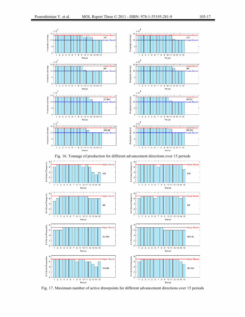
In South to North direction in Fig. 15, it can be seen that the formulation tries to extract high grade slices earlier than others. Fig. 16 shows that tonnage of extraction in South to North direction during the first 11 years is equal to the upper bound of production that has been set up as a scheduling parameter.

X (m)

Y (m)

Hei

ght (

m)


Table 3. Scheduling parameters and obtained net present value

Advancement Direction

/et etG G

(%)

/t tM M

(t)×10

/d t d tDR DR3

(mm/day) atN /nt ntN N NPV

($M)

WE 0.5 / 1.9 100/139 50 / 300 7 0 / 3 2.8074 EW 0.5 / 1.9 100/139 50 / 300 7 0 / 3 2.7649 NS 0.5 / 1.9 100/139 50 / 300 7 0 / 3 2.6936 SN 0.5 / 1.9 100/139 50 / 300 7 0 / 3 2.8497

SE-NW 0.5 / 1.9 100/139 50 / 300 7 0 / 3 2.8019 NW-SE 0.5 / 1.9 100/139 50 / 300 7 0 / 3 2.8033 SW-NE 0.5 / 1.9 100/139 50 / 300 7 0 / 3 2.8280 NE-SW 0.5 / 1.9 100/139 50 / 300 7 0 / 3 2.7210

Fig. 14. Amount of NPV for different directions over 15 years scheduling horizon

Fig. 17 illustrates the maximum number of active drawpoints in each period for the different advancement directions. It can be seen that this constraint has been satisfied for all directions. In South to North direction, the mine works with the maximum allowable number of active drawpoints except for years one, six and fourteen. Fig. 18 illustrates the number of new drawpoints that are opened in each period for all advancement directions.

According toIn South to North direction in Fig. 15, it can be seen that the formulation tries to extract high grade slices earlier than others. Fig. 16 shows that tonnage of extraction in South to North direction during the first 11 years is equal to the upper bound of production that has been set up as a scheduling parameter.

Table 3, the number of new drawpoints that can be opened in each period varies between 0 and 3. As can be seen in Fig. 18, the upper bound is equal to 3 for all periods except period one. In period one, the number of new drawpoints that can be opened is equal to the maximum number of active

Pourrahimian Y. et al. MOL Report Three © 2011 - ISBN: 978-1-55195-281-9 105-16 drawpoints because at the beginning, we need more flexibility to reach the target grade and production level.

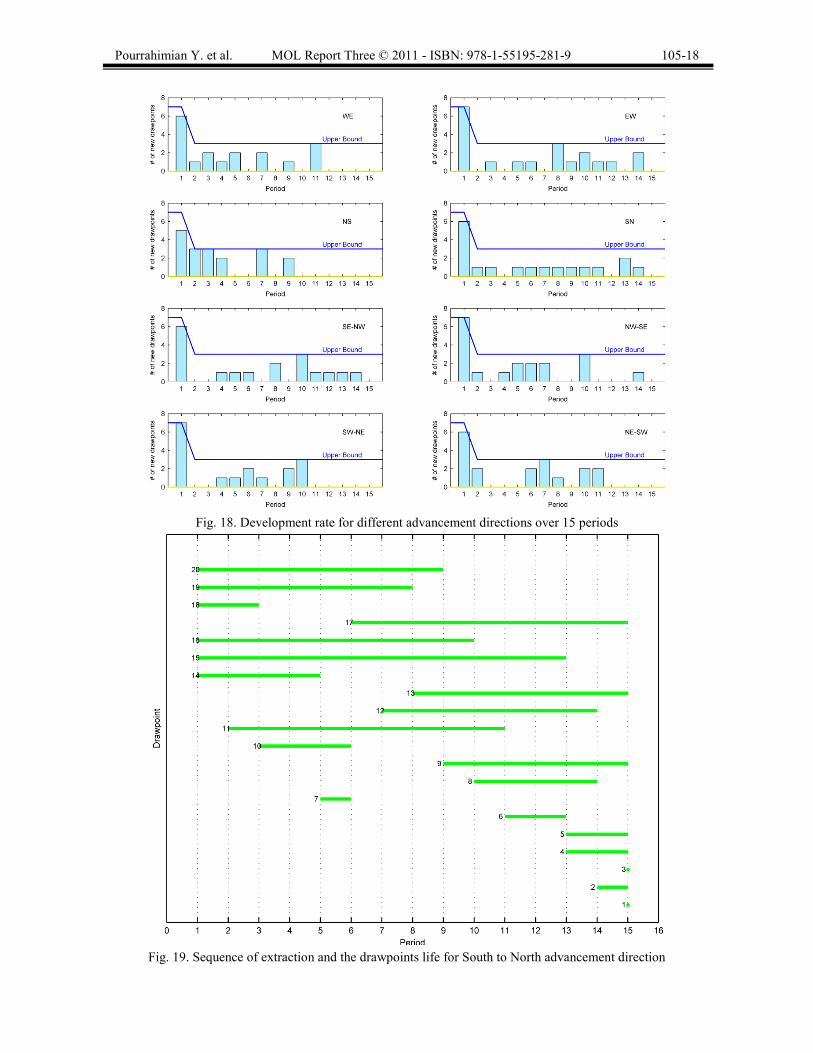
Fig. 18 shows a striking difference in the number of new drawpoints in the different advancement directions. In the South to North direction, extraction starts with six new drawpoints in the first period then the number of new drawpoints falls sharply to two in the second period and it remains almost constant until the end of the mine life. Extraction of all drawpoints is started before period 15 and there is no new drawpoint in this period.

Fig. 19 shows the production schedule for South to North direction. It illustrates the starting and finishing periods of extraction and the drawpoints life during the mine life. The ID number of active drawpoints and new drawpoints can be obtained by comparing Fig. 19 and the South to North direction of Fig. 17 and Fig. 18. For instance, according to the South to North direction of Fig. 17 and Fig. 18, there are seven active drawpoints and one new drawpoint in period five. In Fig. 19, it can be seen that the ID number of active drawpoints include DP7, DP10, DP11, DP15, DP16, DP19 and DP20 and the new drawpoint which has to be opened is DP7.

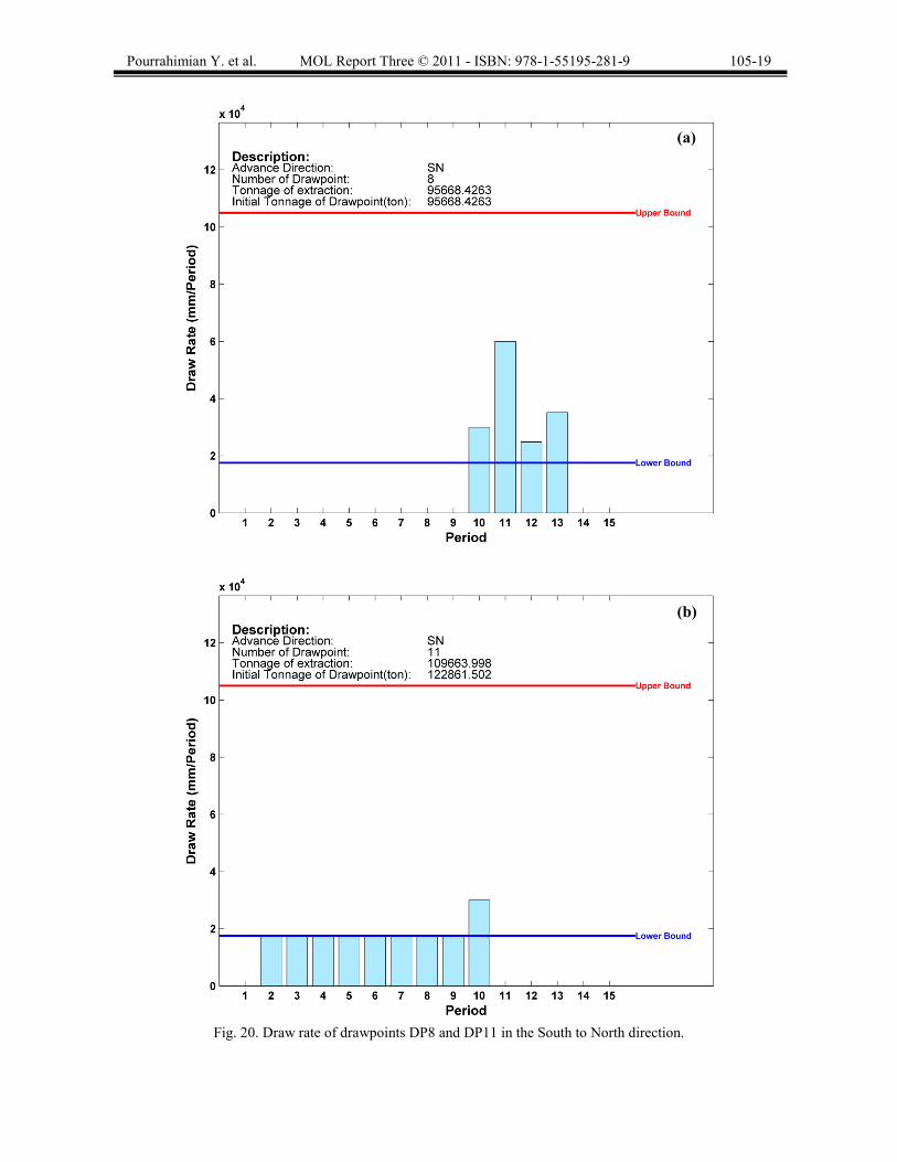
Fig. 20 shows the draw rate for drawpoints DP8 and DP11 in the South to North direction. It can be seen that the defined upper and lower bounds for both selected drawpoints have been satisfied. Fig. 20a shows the fluctuation in the draw rate of DP8; in contrast, Fig. 20b shows that DP11 has an almost uniform draw rate. This situation happened because of constant numbers which have been defined as upper and lower bounds. The formulation tries to extract material from drawpoints with a draw rate within the acceptable range without considering a specific shape.

Fig. 15. Average grade of production for different advancement directions over 15 periods


Fig. 16. Tonnage of production for different advancement directions over 15 periods

Fig. 17. Maximum number of active drawpoints for different advancement directions over 15 periods


Fig. 18. Development rate for different advancement directions over 15 periods

Fig. 19. Sequence of extraction and the drawpoints life for South to North advancement direction


Fig. 20. Draw rate of drawpoints DP8 and DP11 in the South to North direction.

(b)

(a)

Pourrahimian Y. et al. MOL Report Three © 2011 - ISBN: 978-1-55195-281-9 105-20 Fig. 21 shows cumulative tonnage extracted from DP8 and DP11 and percentage of extraction from slices within draw columns associated with drawpoints DP8 and DP11. The Y-axis of Fig. 21a and Fig. 21c represents the ID number of slices within the draw cone associated with the considered drawpoints DP8 and DP11, respectively. The smallest and the biggest numbers in these graphs indicate the lowest and the topmost slices in the draw cone associated with the considered drawpoints. For example, Fig. 21a shows that the lowest and the topmost slices within draw cone associated with drawpoint DP8 are slices 53 and 67, respectively. The blue numbers in these graphs are the percentage of extraction from each slice in the related period. It can be clearly seen that extraction from each slice is started after finishing the extraction of the slice below. Fig. 21b shows that all the material within the draw cone associated with drawpoint DP8 is extracted, while according to Fig. 21d, almost 90 percent of the materials within the draw cone associated with drawpoint DP11 are extracted.

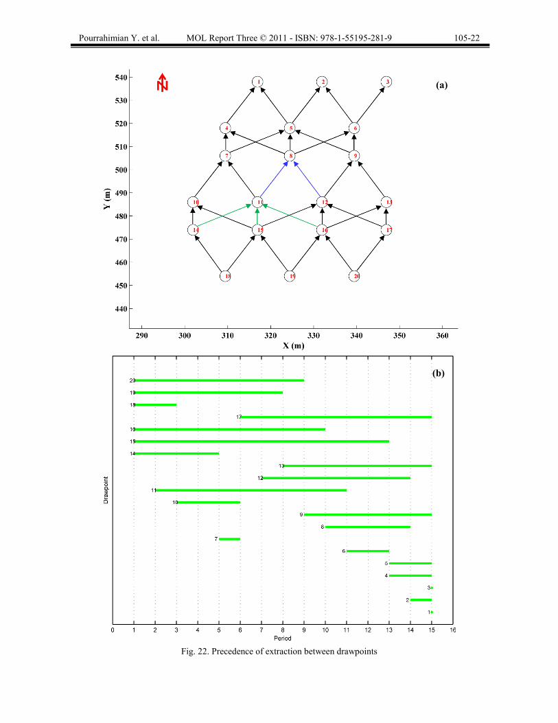
Fig. 22a shows defined precedence among drawpoints for South to North direction based on the mentioned advancement direction concept in Fig. 5 . For example, extraction from drawpoint DP11 can be started if extraction from drawpoints DP14, DP15, and DP16 has been started. Fig. 22b shows obtained start and end periods from the MILP formulation for South to North direction. It can be seen that all defined precedence among drawpoints has been observed. According to Fig. 22a, extraction of drawpoints DP14, DP15, and DP16 can be started after starting the extraction of drawpoints DP18, DP19, and DP20, but Fig. 22b shows that extraction of drawpoints DP14, DP15, DP16, DP18, DP19, and DP20 starts at the same period. This happened because when a small portion of the lowest slices of drawpoints DP18, DP19, and DP20 is extracted that means extraction has been started and extraction of drawpoints DP14, DP15, and DP16 can be started in the same period.

7. Conclusions and future work

The economics of today’s mining industry are such that the major mining companies are increasing the use of massive mining methods. Of the methods available, caving mines are favored because of their low cost and high production rates.

Improvement in both computer processing power and optimization solution algorithms have caused increased ability to find an optimum schedule. These advances have increased the importance of MILP for production scheduling because it can provide a mathematically provable optimum schedule.

This paper presented an MILP formulation for block cave mines production scheduling. The formulation maximizes the NPV subject to several constraints such as development rate, vertical mining rate (production rate per drawpoint), lateral mining rate (rate of opening new drawpoints), mining capacity, ore production target, maximum number of active drawpoints, cave draw strategies and advancement direction. The production scheduler defines the following: the opening and closing time of each drawpoint, the draw rate from each drawpoint, the number of new drawpoints that need to be constructed, and the sequence of extraction from the drawpoints to support a given production target.

Further focused research is underway to add new capabilities to the model. In the presented model, constant draw rates were used as upper and lower bounds. One method of managing drawpoint production is by establishing a production rate curve, which limits production based on the amount of material that has been drawn previously. This means that production depends on the cumulative tonnes mined from a drawpoint. So in the new model production rate curve (PRC) will be used instead of the constant upper and lower boundaries. Sometimes extraction from drawpoints is started from two or more different areas of the mine; hence we need to have a schedule which considers all mining areas at the same time. For this reason, some new constraint will be added to the MILP formulation for handling multiple-lift and multiple-mine scenarios.


Fig. 21. Cumulative depletion tonnage and extraction percent from slices of DP8 and DP11 in South to North

direction

(a)

(c)

(b)

(d)


Fig. 22. Precedence of extraction between drawpoints

(a)

(b)

Pourrahimian Y. et al. MOL Report Three © 2011 - ISBN: 978-1-55195-281-9 105-23 8. References

[1] Ataee-Pour, M. (2005). A critical suvey of existing stope layout optimisation technique. Journal of Mining Science, 41 (5), 447-466.

[2] Brown, E. T. (2003). Block caving geomechanics. Indooroopilly, Queensland : Julius Kruttschnitt Mineral Researh Centre, The University of Queensland, Pages 516.

[3] Carew, t. (1992). The casier mine case study. in Proceedings of MassMin 1992, Johannesburg,

[4] Carlyle, W. M. and Eaves, B. C. (2001). Underground planning at Stillwater mining company. INTERFACES, 31 (4), 50-60.

[5] Chanda, E. C. K. (1990). An application of integer programming and simulation to production planning for a stratiform ore body. Mining Science and Technology, 11 (1), 165-172.

[6] Dewolf, V. (1981). Draw control in principle and practice at Henderson mine. in Design and operation of caving and sublevel stoping mines, D. R. Steward, Ed. New York, Society of Mining Engineers of AIME., pp. 729-735.

[7] Diering, T. (2000). PC-BC: A block cave design and draw control system. in Proceedings of MassMin 2000, The Australasian Institute of mining and Metallurgy: melburne, brisbane, pp. 301-335.

[8] Diering, T. (2004). Computational considerations for production scheduling of block vave mines. in Proceedings of MassMin 2004, Santiago, Chile, pp. 135-140.

[9] GEMCOMSoftwareInternational (2011). Ver. 6.2.4, Vancouver, BC, CANADA.

[10] Guest, A., Van Hout, G. J., Von Johannides, A., and Scheepers, L. F. (2000). An application of linear programming for block cave draw control. in Proceedings of Massmin2000, The australian Institute of Mining and Metallurgy: Melbourne., Brisbane,

[11] Heslop, T. G. and Laubscher, D. H. (1981). Draw control in caving operations on Southern African Chrpsotile Asbestos mines. in Design and operation of caving and sublevel stoping mines, New York, Society of Mining Engineers of AIME., pp. 755-774.

[12] Holmstrom, K. (1989-2009). TOMLAB/CPLEX, ver. 11.2. Ver. Pullman, WA, USA: Tomlab Optimization.

[13] Holmström, K. (1989-2009). TOMLAB /CPLEX - v11.2. Ver. Pullman, WA, USA.

[14] Horst, R. and Hoang, T. (1996). Global optimization : deterministic approaches. Springer, New York, 3rd ed, Pages xviii, 727 p.

[15] ILOGInc (2007). ILOG CPLEX 11.0 User’s Manual. Ver. 11.0, ILOG S.A. and ILOG, Inc.

[16] Jawed, M. (1993). Optimal production planning in underground coal mines through goal programming-A case stydy from an Indian mine. in Proceedings of 24th international symposium, Application of computers in the mineral industry(APCOM), Montreal,Quebec, Canada, pp. 43-50.

[17] Kuchta, M., Newman, A., and Topal, E. (2004). Implementing a Production Schedule at LKAB 's Kiruna Mine. Interfaces, 34 (2), 124-134.

[18] MathWorksInc (2007). MATLAB (R2009b). Ver. 7.9.0.529, MathWorks, Inc.

[19] McIssac, G. (2005). Long term planning of an underground mine using mixed integer linear programming. in CIM Bulletin, vol. 98, pp. 89.

Pourrahimian Y. et al. MOL Report Three © 2011 - ISBN: 978-1-55195-281-9 105-24 [20] Ovanic, J. (1998). Economic optimization of stope geometry. PhD Thesis, Michigan

Technological University, Houghton, USA, Pages 209.

[21] Pourrahimian, Y. and Askari-Nasab, H. (2010). A mathematical programming formulation for block cave production scheduling. University of Alberta, Mining Optimization Laboratory (MOL) 2nd report, pp. 134-156.

[22] Rahal, D., Smith, M., Van Hout, G. J., and Von Johannides, A. (2003). The use of mixed integer linear programming for long-term scheduling in block caving mines. in Proceedings of 31st International Symposium on the Application of Computers and operations Research in the Minerals Industries (APCOM), Cape Town, South Africa,

[23] Riddle, J. (1976). A dynamic programming solution of a block caving mine layout. in Proceedings of 14th International Symposium on the Application of Computers in the Mineral Industry(APCOM), Pennsylvania,

[24] Rubio, E. (2002). Long-term planning of block caving operations using mathematical programming tools. MSc Thesis, Vancouver, Canada, Pages 116.

[25] Rubio, E., Caceres, C., and Scoble, M. (2004a). Towards an integrated approach to block cave planning. in Proceedings of MassMin 2004, Santiago, Chile, pp. 128-134.

[26] Sarin, S. C. and West-Hansen, J. (2005). The long-term mine production scheduling problem. IIE Transactions, 37 (2), 109-121.

[27] Tang, X., Xiong, G., and Li, X. (1993). An integrated approach to underground gold mine planning and sheduling optimization. in Proceedings of 24th international symposium on the Application of computers in the mineral industry(APCOM), Montreal, Quebec, Canada, pp. 148-154.

[28] Topal, E. (2008). Early start and late start algorithms to improve the solution time for long-term underground mine production scheduling. Journal of The South African Institute of Mining and Metallurgy, 108 (2), 99-107.

[29] Topal, E., Kuchta, M., and Newman, A. (2003). Extensions to an efficient optimization model for long-term production planning at LKAB’s Kiruna Mine. in Proceedings of APCOM 2003, Cape Town, South Africa, pp. 289-294.

[30] Trout, L. P. (1995). Underground mine production scheduling using mixed integer programming. in Proceedings of 25th international symposium, Application of computers in the mineral industry(APCOM), Brisbane, Australia, pp. 395-400.

[31] Williams, J., Smith, L., and Wells, M. (1972). Planning of underground copper mining. in Proceedings of 10th international symposium, Application of computers in the mineral industry(APCOM), Johannesburg, South Africa, pp. 251-254.

[32] Winkler, B. M. (1998). Mine production scheduling using linear programming and virtual reality. in Proceedings of 27th international symposium, Application of computers in the mineral industry(APCOM), Royal school of mines, London, United Kingdom, pp. 663-673.

[33] Winston, W. L. (1995). Introduction to mathematical programming : applications and algorithms. Duxbury Press, 2nd ed, Pages xv, 818, 39 p.

9. Appendix

MATLAB and TOMLAB/CPLEX documentation for block cave mines scheduling

http://www.ualberta.ca/MOL/locked-dir/DataFiles/2011_Papers/Doc/105/index.html

block cave production scheduling optimization using mixed

Documents