bmc bioinformatics biomed central bioinformatics research article open access the statistics of...

BioMed CentralBMC Bioinformatics

ss
Open AcceResearch articleThe statistics of identifying differentially expressed genes in Expresso and TM4: a comparisonAllan A Sioson1, Shrinivasrao P Mane2, Pinghua Li3, Wei Sha4, Lenwood S Heath*1, Hans J Bohnert3 and Ruth Grene2
Address: 1Department of Computer Science, Virginia Tech, Blacksburg, USA, 2Department of Plant Pathology, Physiology and Weed Science, Virginia Tech, Blacksburg, USA, 3Department of Plant Biology and Department of Crop Sciences, University of Illinois, Urbana, USA and 4Virginia Bioinformatics Institute, Virginia Tech, Blacksburg, USA

Email: Allan A Sioson - [email protected]; Shrinivasrao P Mane - [email protected]; Pinghua Li - [email protected]; Wei Sha - [email protected]; Lenwood S Heath* - [email protected]; Hans J Bohnert - [email protected]; Ruth Grene - [email protected]

* Corresponding author

AbstractBackground: Analysis of DNA microarray data takes as input spot intensity measurements from scannersoftware and returns differential expression of genes between two conditions, together with a statisticalsignificance assessment. This process typically consists of two steps: data normalization and identificationof differentially expressed genes through statistical analysis. The Expresso microarray experimentmanagement system implements these steps with a two-stage, log-linear ANOVA mixed model technique,tailored to individual experimental designs. The complement of tools in TM4, on the other hand, is basedon a number of preset design choices that limit its flexibility. In the TM4 microarray analysis suite,normalization, filter, and analysis methods form an analysis pipeline. TM4 computes integrated intensityvalues (IIV) from the average intensities and spot pixel counts returned by the scanner software as inputto its normalization steps. By contrast, Expresso can use either IIV data or median intensity values (MIV).Here, we compare Expresso and TM4 analysis of two experiments and assess the results against qRT-PCRdata.

Results: The Expresso analysis using MIV data consistently identifies more genes as differentiallyexpressed, when compared to Expresso analysis with IIV data. The typical TM4 normalization and filteringpipeline corrects systematic intensity-specific bias on a per microarray basis. Subsequent statistical analysiswith Expresso or a TM4 t-test can effectively identify differentially expressed genes. The best agreementwith qRT-PCR data is obtained through the use of Expresso analysis and MIV data.

Conclusion: The results of this research are of practical value to biologists who analyze microarray datasets. The TM4 normalization and filtering pipeline corrects microarray-specific systematic bias andcomplements the normalization stage in Expresso analysis. The results of Expresso using MIV data havethe best agreement with qRT-PCR results. In one experiment, MIV is a better choice than IIV as input todata normalization and statistical analysis methods, as it yields as greater number of statistically significantdifferentially expressed genes; TM4 does not support the choice of MIV input data. Overall, the moreflexible and extensive statistical models of Expresso achieve more accurate analytical results, when judgedby the yardstick of qRT-PCR data, in the context of an experimental design of modest complexity.

Published: 20 April 2006

BMC Bioinformatics 2006, 7:215 doi:10.1186/1471-2105-7-215

Received: 16 August 2005Accepted: 20 April 2006

This article is available from: http://www.biomedcentral.com/1471-2105/7/215

© 2006 Sioson et al; licensee BioMed Central Ltd.This is an Open Access article distributed under the terms of the Creative Commons Attribution License (http://creativecommons.org/licenses/by/2.0), which permits unrestricted use, distribution, and reproduction in any medium, provided the original work is properly cited.

of 15(page number not for citation purposes)

http://www.biomedcentral.com/1471-2105/7/215

http://creativecommons.org/licenses/by/2.0

http://www.ncbi.nlm.nih.gov/entrez/query.fcgi?cmd=Retrieve&db=PubMed&dopt=Abstract&list_uids=16626497

http://www.biomedcentral.com/

http://www.biomedcentral.com/info/about/charter/

BMC Bioinformatics 2006, 7:215 http://www.biomedcentral.com/1471-2105/7/215

BackgroundDNA microarrays are a powerful means of monitoring theexpression of thousands of genes simultaneously. A vari-ety of computational and statistical methods have beenproposed to extract information from the large quantity ofdata generated from microarray experiments. Many meth-ods assume, as we do here, the use of cDNA labeled withone of two fluorescent dyes to differentiate two treatmentson a single microarray, implying data from two images tobe analyzed. These methods include a number of datanormalization techniques to reduce the effects of system-atic errors and various kinds of statistical tests to identifydifferentially expressed genes in comparisons among dif-ferent experimental conditions. There is as yet no singlemethod that can be recommended under all circum-stances for either normalization or identification of differ-ential gene expression.

In recent years, ANOVA methods have gained popularityfor identification of differential gene expression. Thepower of ANOVA methods derives from their flexibility infitting and comparing different models to a given set ofdata [1]. One such method is the two-stage, log-linearANOVA mixed models technique of Wolfinger, et al., [2].Its first stage uses a normalization model designed toremove global effects across all microarrays. Its secondstage uses a gene-specific model to estimate gene-treat-ment interactions as ratios of gene expression under con-trol and treated conditions, along with a statisticalsignificance. Kerr [3] notes that the global normalizationmodel employed in this technique is conducive to com-bining data across genes for realistic and robust models oferror, especially when random effects are included. Pan[4] compares different microarray statistical analysismethods and demonstrates that the log-linear ANOVAmixed model approach performs better than the t-test andregression approaches. The regression approach, althoughflexible and robust, assumes that the data is drawn from anormal distribution, while the t-test is limited due to veryfew degrees of freedom. Chu, et al., [5] compare two log-linear ANOVA mixed models for probe-level, oligonucle-otide array data and found that both types of models cap-ture key measurable sources of variability ofoligonucleotide arrays for real and simulated data. Cuiand Churchill [6] review the use of a mixed ANOVAmodel for analyzing a cDNA microarray experiment andconclude that such models provide a powerful way toobtain information from experiments with multiple fac-tors or sources of variation. Rosa, et al., [7] review issuesof analyzing cDNA microarrays with mixed linear modelsand puts such analysis in the larger context of Bayesiananalysis procedures and adjustments for multiple testing.

Data normalization is the first step in analyzing microar-ray data; numerous data normalization methods have

been proposed and investigated. While refinements ofexisting methods continue to appear (e.g., Futschik andCrompton [8]), naive methods, such as total intensitynormalization, are still in use (e.g., Held, et al., [9]). Xie,et al., [10] did a comparative study of normalizationmethods and test statistics to analyze the results of a DNA-protein binding microarray experiment. Using perform-ance and bias correction criteria, Bolstad, et al., [11] eval-uate the cyclic lowess method, the contrast method, thequantile method, and baseline array scaling methods,both linear and non-linear; they demonstrate that nor-malization methods incorporating data from all microar-rays perform better than methods employing a baselinearray.

Several software tools that combine data normalizationand statistical analysis are currently available. Dudoit, etal., [12] review these software tools with an emphasis onthe TM4 microarray software suite, Bioconductor in R,and the BioArray Software Environment (BASE) system.Saeed, et al., [13] describe the features and capabilities ofTM4, while Quackenbush [14] describes the normaliza-tion and transformation methods implemented in it. Wil-liams, et al., [15], Zhu, et al., [16], and Khaitovich, et al.,[17] have used TM4 in microarray data analysis. Anothersystem is Expresso, an experiment management systemthat serves as a unifying framework to study data drivenapplications such as microarray experiments [18-20].Expresso has adapted the two-stage ANOVA mixed mod-els technique of Wolfinger, et al., [2] to the particularneeds of individual microarray data sets. Our experiencewith numerous such data sets has demonstrated thatmodeling the underlying experiment carefully and com-pletely is essential to obtaining meaningful and defensi-ble results. Use of tools that require experiments toconform to their analysis methods are less than satisfac-tory.

In this paper, we compare the Expresso analysis method-ology to the approach provided in the TM4 microarrayanalysis software suite [13]. Each is invoked to identifydifferentially expressed genes in two experimental datasets, each of which uses an Arabidopsis thaliana oligonucle-otide array. Along the way, we demonstrate differencesbetween the use of integrated intensity values (IIV) andmedian intensity values (MIV) as inputs. We report inter-actions between normalization and gene identificationmethods. We use quantitative reverse-transcriptase PCR(qRT-PCR) results to assess the consistency of genesreported by TM4 and Expresso as having significant differ-ential expression.

Results and discussionHere, we report a portion of the results obtained in ourcomparison of Expresso analysis and the TM4 pipeline



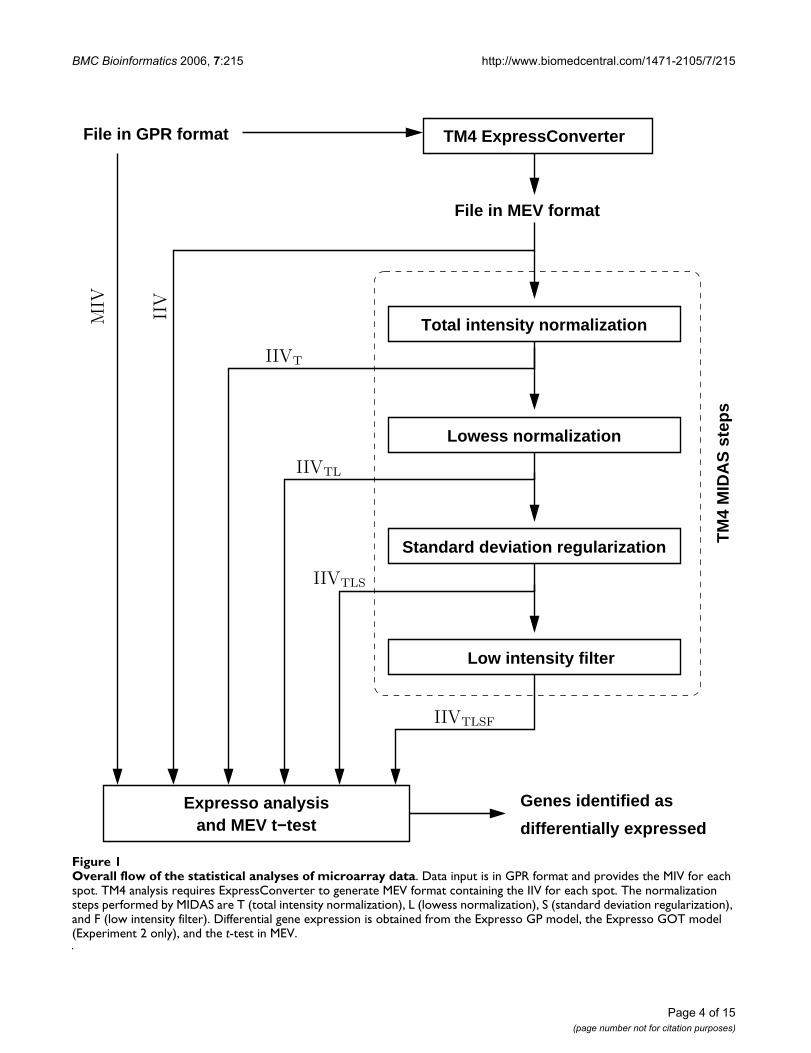
(see Materials and Methods). Figure 1 illustrates the over-all flow of the statistical analyses of microarray data thatwere done in this study. We began with microarray data inGPR format from Experiment 1 and Experiment 2.Median intensity values (MIV) from the GPR files can beanalyzed by the Expresso GP and GOT models directly.ExpressConverter provides integrated intensity values(IIV) for further Expresso and TM4 analysis. The MIDASnormalization and filtering pipeline executes these stepsin order: total intensity normalization (subscript T), low-ess normalization (subscript L), standard deviation regu-larization (subscript S), and low intensity filter (subscriptF). MIDAS allows tapping the output of any step in thepipeline; for example, IIVTL signifies an MEV file after totalintensity normalization followed by lowess normaliza-tion. The identification of genes with significant differen-tial expression was performed on all GPR and MEV files,using the Expresso GP and GOT models and the t-test inMEV.

Normalization and low intensity filtering in TM4Quackenbush [14] describes the use of ratio-intensityplots (RI-plots) to detect and normalize for any systematicintensity-dependent dye bias using lowess normalization(see Materials and Methods). We evaluated the effect oflowess normalization within the context of the flow inFigure 1 by creating RI-plots after each step for the secondreplicate microarray in Experiment 1, WT plant. Supple-mentary Figure 1 - see Additional file: 1 contains these RI-plots. The IIVTL is indeed effective, for this data set, in cor-recting systematic dye bias, suggesting that preprocessingby these two normalization steps in MIDAS may be agood practice in many situations.

The normalization and filtering pipeline affects thenumber of genes identified as differentially expressed inboth the GP and GOT models. See Table 1. For example,in Experiment 1, the GP model using IIV input data iden-tifies 567 up-expressed genes in the WT microarrays, whileit identifies only 460 WT genes as up-expressed if IIVTLSF(processed by the complete MIDAS pipeline) input data isused.

Small changes in the number of genes identified as up- ordown-expressed after successive MIDAS steps may masklarger changes in the composition of sets of up- anddown-expressed genes. To obtain a more precise view ofthe effects of MIDAS changes, we computed retentioncounts (RC) and retention percentages (RP) between thegene successive sets whose numbers are in Table 1. RC isthe number of genes in the set before the MIDAS step thatremain in the set after the step. RP is the percentage ofremaining genes with respect to the number of genes inthe set after the MIDAS step. Table 2 contains the RC andRP values corresponding to the counts in Table 1. For

Experiment 1, there is a tremendous drop in retentionduring the lowess normalization that follows the totalintensity normalization. There is not a drop of corre-sponding magnitude for Experiment 2. For both experi-ments, normalization has a significant effect on the sets ofgenes identified as differentially expressed.

In Experiment 1 results, the number of genes commonlyassessed by Expresso as significantly expressed when usingIIV and IIVT is high. For example, there is 95.45% reten-tion of WT genes (545 total) assessed as up-expressedwhen using IIVT data in Expresso compared to that whenusing IIV data. Retention percentage of these genesassessed as expressed however went down after doing low-ess normalization. There is only 15.20% retention of WTgenes (74 total) assessed as up-expressed in the resultswhen using IIVTS data in Expresso compared to whenusing IIVT. While we observe increase in the retention per-centage in IIVTLS (from IIVTL) and IIVTLSF (from IIVTLS),there's low retention percentage in the results using IIVTLSFfrom IIV data. This can be traced in the low retention per-centage of IIVTL from IIVT. Hence, the normalizationmethod that affects the results in Experiment 1 the most islowess normalization.

The results of Expresso on Experiment 2 show that lowretention percentages happen after appli-cation of totalintensity normalization (lowest is 59.30%) and afterapplication of low intensity filtering (lowest is 61.19%).The low retention percentages shown in the IIV ∩ IIVTLSFcolumn implies that the normalization pipeline also sig-nificantly affects the results in Expresso analysis of Exper-iment 2.

Choice of intensity signal dataThe input to statistical analysis of microarray experimentsis a set of real numbers that represent the measured inten-sity signal for each spot in a microarray. Much statisticalanalysis of microarray data has traditionally used medianintensity values (MIV). The alternative used in TM4 is theintegrated intensity value (IIV). (See Materials and Meth-ods.) Since IIV is intended to integrate the measuredintensity across the biological sample printed at a spot,one might expect IIV to be a more accurate assessment ofthe biological measurement than MIV data. For example,a spot having 100 pixels and a median intensity of 5,000has the same IIV as a spot having 50 pixels and a medianintensity of 10,000.

This study provides the opportunity to observe the differ-ence that choosing MIV or IIV makes on the sets of genesultimately identified as differentially expressed. We usedthe GP model to analyze unnormalized MIV and IIV datafrom Experiment 1, and we used the GOT model to ana-lyze unnormalized MIV and IIV data from Experiment 2.




Overall flow of the statistical analyses of microarray dataFigure 1Overall flow of the statistical analyses of microarray data. Data input is in GPR format and provides the MIV for each spot. TM4 analysis requires ExpressConverter to generate MEV format containing the IIV for each spot. The normalization steps performed by MIDAS are T (total intensity normalization), L (lowess normalization), S (standard deviation regularization), and F (low intensity filter). Differential gene expression is obtained from the Expresso GP model, the Expresso GOT model (Experiment 2 only), and the t-test in MEV.

Low intensity filter

Standard deviation regularization

Total intensity normalization

Lowess normalization

TM

4 M

IDA

S s

tep

s

File in MEV format

File in GPR format

Expresso analysis Genes identified as

differentially expressed

TM4 ExpressConverter

and MEV t−test

IIVTLSF

IIVT

IIVTL

IIVTLS

IIV

MIV


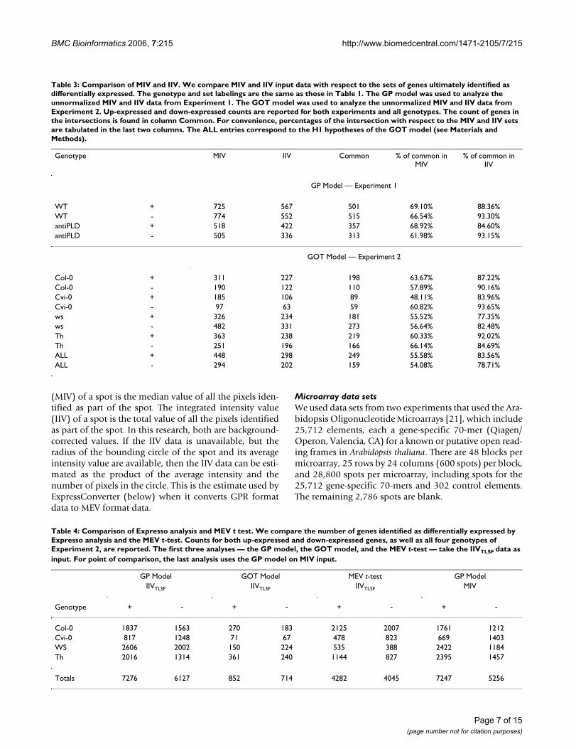
Table 3 reports a summary of the results. In Experiment 1,725 WT genes are assessed as up-expressed and 774 WTgenes are down-expressed when MIV data are used inExpresso. These numbers decreased to 567 up-expressedgenes and 552 down-expressed genes when IIV data areused instead. A similar trend is observed in Experiment 2results when using MIV and IIV data. These results suggestthat employing IIV input data with Expresso analysis leadsto more conservative results than employing MIV inputdata.

Comparison of statistical methodsWe compared the performance of the GP model, the GOTmodel, and the t-test of MEV in identifying differentiallyexpressed genes in Experiment 2. We used the IIVTLSF dataof Experiment 2 as input to these methods. We also con-trast these results with MIV data analyzed in GP. Table 4reports counts for these analyses.

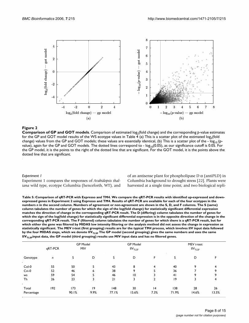
The plot in Figure 2a demonstrates that the estimates ofIog2(fold change) are the same in GP and GOT. As Figure2b shows, the p values by GOT are smaller compared tothe p values calculated by GP. Use of the MEV t-testresulted in fewer genes assessed as significantly expressedwhen compared to the numbers for the GP model. Theresults obtained when MIV data was used as input to GP,is closest to the results when using IIVTLSF.

To compare the effectiveness of Expresso and TM4 inidentifying gene differential expression, we compared theidentified direction of differential expression of a select setof genes per genotype in Experiment 2 with resultsobtained by qRT-PCR. See Table 5. The lowest overall per-centage (71.9%) of agreement is between the qRT-PCRresults and the MEV t-test results using IIVTLSF. Thelog(fold change) estimates of the GP model has 77.1%percentage agreement with the qRT-PCR results, which isslightly higher than the percentage for the MEV t-test. Theresults of the GP model using MIV data demonstrated thegreatest agreement, 90.1%, with the qRT-PCR results.

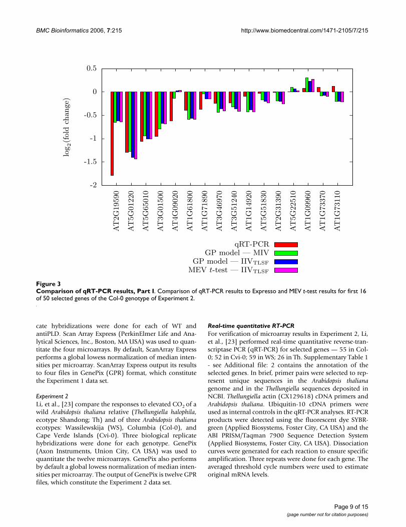
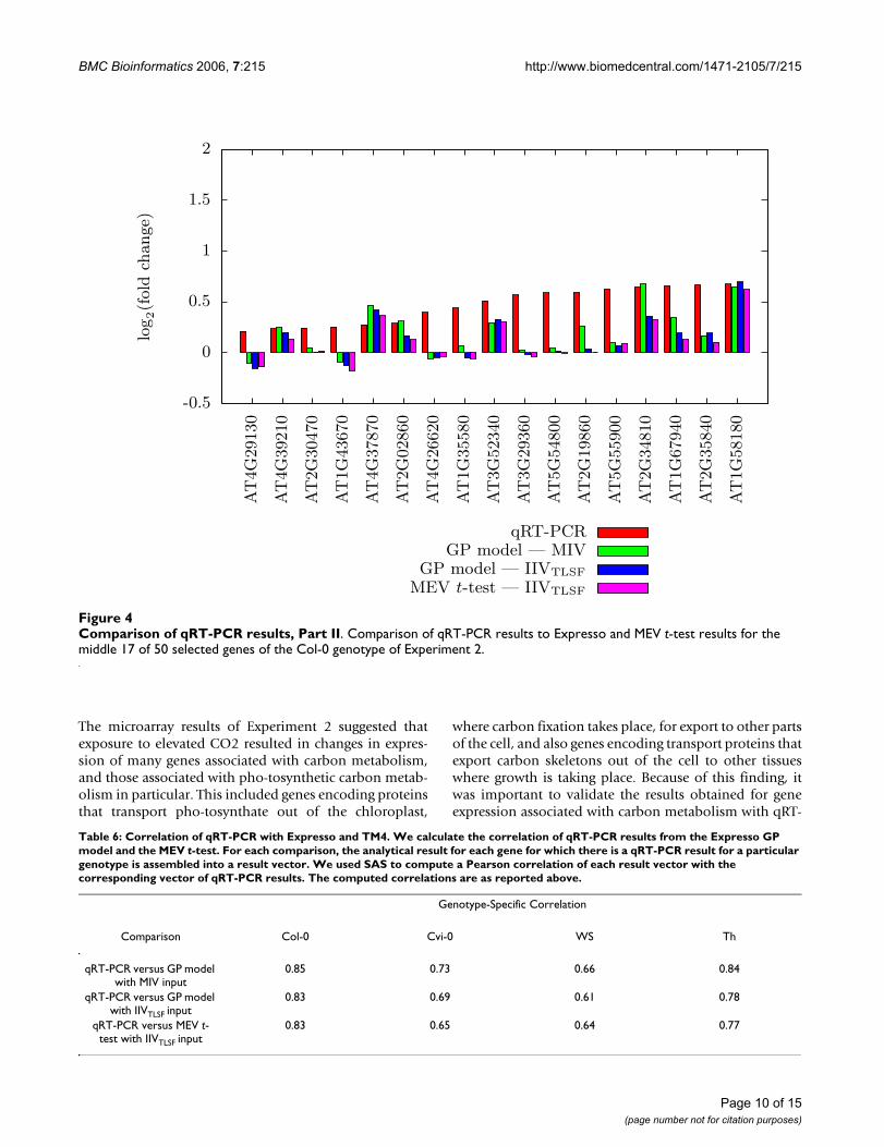
Figures 3, 4, and 5 present the actual assessed Iog2(foldchange) values for 50 selected Col-0 genes in Experiment2, along with their qRT-PCR values. These are the 50 Col-0 genes, among the 55 with qRT-PCR values, for which wehave expression values for all methods. For each gene, ahistogram of the Iog2(fold change) estimates of qRT-PCR,the GP model using MIV, the GP model using IIVTLSF, andthe MEV t-test is given. The 50 histograms are spread overthree figures to enhance readability and are in increasingorder by qRT-PCR estimated change. In general, thelog2(fold change) estimates of the GP model and of theMEV t-test, all IIVTLSF input data, are approximately thesame, while being slightly different from estimates of theGP model using MIV input data. As might be expected,disagreement between qRT-PCR and microarray resultsare more prevalent for small estimated log2(fold change)

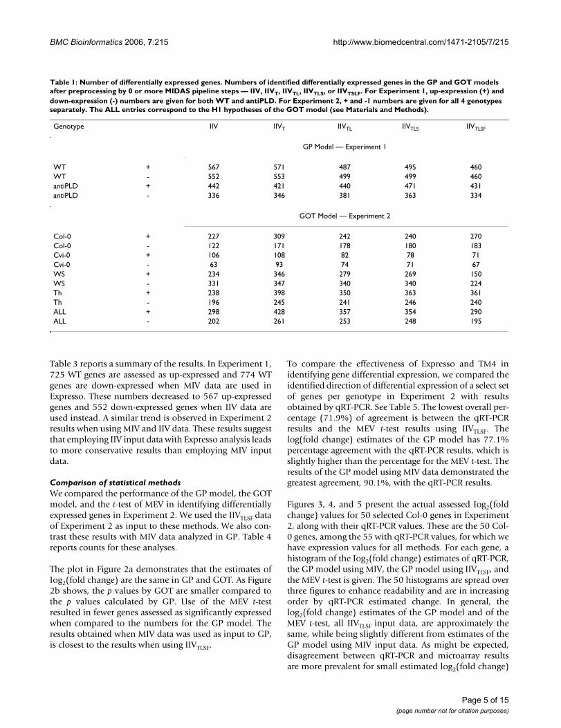
Table 1: Number of differentially expressed genes. Numbers of identified differentially expressed genes in the GP and GOT models after preprocessing by 0 or more MIDAS pipeline steps — IIV, IIVT, IIVTL, IIVTLS, or IIVTSLF. For Experiment 1, up-expression (+) and down-expression (-) numbers are given for both WT and antiPLD. For Experiment 2, + and -1 numbers are given for all 4 genotypes separately. The ALL entries correspond to the H1 hypotheses of the GOT model (see Materials and Methods).

Genotype IIV IIVT IIVTL IIVTLS IIVTLSF

GP Model — Experiment 1

WT + 567 571 487 495 460WT - 552 553 499 499 460antiPLD + 442 421 440 471 431antiPLD - 336 346 381 363 334

GOT Model — Experiment 2

Col-0 + 227 309 242 240 270Col-0 - 122 171 178 180 183Cvi-0 + 106 108 82 78 71Cvi-0 - 63 93 74 71 67WS + 234 346 279 269 150WS - 331 347 340 340 224Th + 238 398 350 363 361Th - 196 245 241 246 240ALL + 298 428 357 354 290ALL - 202 261 253 248 195



values. The histograms for genes AT4G09020 (Figure 3),AT1G35580 (Figure 4), and AT3G29360 (Figure 4) showthat the direction of log(fold change) estimate of qRT-PCR matches the direction of the GP model using MIVinput data, while differing from the direction of the esti-mates of the GP model and the MEV t-test using IIVTLSFinput data.

Table 6 summarizes genotype-specific correlation results,which demonstrate that the GP model us-ing MIV inputdata has the highest correlation with qRT-PCR comparedto the GP model and the MEV t-test using IIVTLSF inputdata. The highest correlation of 0.85 is for the Col-0results of qRT-PCR versus the GP model using MIV input.The corresponding correlations for Cvi-0, WS, and Th are0.73, 0.66, and 0.84, respectively, which are all bestamong the analysis methods.

ConclusionOur integration and comparison of Expresso analysis andthe capabilities of TM4 has highlighted successes inmicroarray analysis, some similarities, and some differ-ences. The success of microarray analysis is demonstratedby considerable agreement between qRT-PCR results andthe results of all the examined microarray analysis meth-ods. The greatest agreement was found when median

intensity value (MIV) inputs were analyzed with theExpresso GP analysis model. We also found that the use ofintegrated intensity value (IIV) inputs for Expresso analy-sis consistently resulted in fewer genes identified as differ-entially expressed when compared to results from MIVinputs. This suggests that the use of IIV inputs is more con-servative than the use of MIV inputs, while MIV inputsmay give greater agreement to qRT-PCR results than IIVinputs.

Our results demonstrate that the MIDAS normalizationand filtering pipeline corrects systematic intensity-dependent dye bias on a per microarray basis. The nor-malization stage in Expresso analysis removes globaleffects across all microarrays and complements the permicroarray normalization methods of MIDAS. The gener-ally better agreement of Expresso analysis with qRT-PCRresults when compared to the MEV t-test suggests that itwould be desirable for MEV to have an ANOVA test thathas the greater flexibility of the Expresso gene model.

MethodsMedian and integrated intensity valuesThis research considers two ways of measuring spot inten-sity, one or both of which are reported by typical microar-ray image processing software. The median intensity value

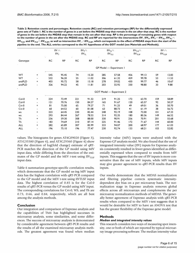
Table 2: Retention counts and percentages. Retention counts (RC) and retention percentages (RP) for the differentially expressed gene sets of Table 1. RC is the number of genes in a set before the MIDAS step that remain in the set after that step. RC is the number of genes in the set before the MIDAS step that remain in the set after that step. RP is the percentage of remaining genes with respect to the number of genes in the set after the MIDAS step. RC and RP are reported for the intersections IIV∩ IIVT, IIVT ∩ IIVTL, IIVTL ∩ IIVTLS, and IIVTLS ∩ IIVTLSF, as well as intersection IIV∩ ∩IIVTLSF, which corresponds to the effect of MIDAS steps from the start of the pipeline to the end. The ALL entries correspond to the H1 hypotheses of the GOT model (see Materials and Methods).

IIV ∩ IIVT∩ IIVTL∩ IIVTLS∩ IIV ∩IIVT IIVTL IIVTLS IIVTLSF IIVTLSF

Genotype RC RP RC RP RC RP RC RP RC RP


WT + 545 95.45 74 15.20 285 57.58 456 99.13 59 12.83WT - 532 96.20 55 11.02 306 61.32 459 99.78 53 11.52antiPLD + 403 95.72 58 13.18 278 59.02 430 99.77 46 10.67antiPLD - 326 94.22 45 11.81 203 55.92 330 98.80 33 9.88


Col-0 + 224 72.49 221 91.32 219 91.25 172 63.70 159 58.89Col-0 - 121 70.76 150 84.27 165 91.67 120 65.57 92 50.27Cvi-0 + 81 75.00 65 79.27 71 91.25 49 69.01 36 50.70Cvi-0 - 60 64.52 60 81.08 63 88.73 41 61.19 38 56.72ws + 223 64.45 230 82.44 248 92.19 108 72.00 101 67.33ws - 293 84.44 267 78.53 314 92.35 180 80.36 149 66.52Th + 236 59.30 308 88.00 330 90.91 256 70.91 201 55.68Th - 183 74.69 210 87.14 225 91.46 172 71.67 144 60.00ALL + 282 65.89 307 85.99 333 94.07 200 68.97 177 61.03ALL - 196 75.10 196 77.47 230 92.74 133 68.21 103 52.82



(MIV) of a spot is the median value of all the pixels iden-tified as part of the spot. The integrated intensity value(IIV) of a spot is the total value of all the pixels identifiedas part of the spot. In this research, both are background-corrected values. If the IIV data is unavailable, but theradius of the bounding circle of the spot and its averageintensity value are available, then the IIV data can be esti-mated as the product of the average intensity and thenumber of pixels in the circle. This is the estimate used byExpressConverter (below) when it converts GPR formatdata to MEV format data.

Microarray data setsWe used data sets from two experiments that used the Ara-bidopsis Oligonucleotide Microarrays [21], which include25,712 elements, each a gene-specific 70-mer (Qiagen/Operon, Valencia, CA) for a known or putative open read-ing frames in Arabidopsis thaliana. There are 48 blocks permicroarray, 25 rows by 24 columns (600 spots) per block,and 28,800 spots per microarray, including spots for the25,712 gene-specific 70-mers and 302 control elements.The remaining 2,786 spots are blank.

Table 3: Comparison of MIV and IIV. We compare MIV and IIV input data with respect to the sets of genes ultimately identified as differentially expressed. The genotype and set labelings are the same as those in Table 1. The GP model was used to analyze the unnormalized MIV and IIV data from Experiment 1. The GOT model was used to analyze the unnormalized MIV and IIV data from Experiment 2. Up-expressed and down-expressed counts are reported for both experiments and all genotypes. The count of genes in the intersections is found in column Common. For convenience, percentages of the intersection with respect to the MIV and IIV sets are tabulated in the last two columns. The ALL entries correspond to the H1 hypotheses of the GOT model (see Materials and Methods).

Genotype MIV IIV Common % of common in MIV

% of common in IIV


WT + 725 567 501 69.10% 88.36%WT - 774 552 515 66.54% 93.30%antiPLD + 518 422 357 68.92% 84.60%antiPLD - 505 336 313 61.98% 93.15%


Col-0 + 311 227 198 63.67% 87.22%Col-0 - 190 122 110 57.89% 90.16%Cvi-0 + 185 106 89 48.11% 83.96%Cvi-0 - 97 63 59 60.82% 93.65%ws + 326 234 181 55.52% 77.35%ws - 482 331 273 56.64% 82.48%Th + 363 238 219 60.33% 92.02%Th - 251 196 166 66.14% 84.69%ALL + 448 298 249 55.58% 83.56%ALL - 294 202 159 54.08% 78.71%

Table 4: Comparison of Expresso analysis and MEV t test. We compare the number of genes identified as differentially expressed by Expresso analysis and the MEV t-test. Counts for both up-expressed and down-expressed genes, as well as all four genotypes of Experiment 2, are reported. The first three analyses — the GP model, the GOT model, and the MEV t-test — take the IIVTLSF data as input. For point of comparison, the last analysis uses the GP model on MIV input.

GP Model GOT Model MEV t-test GP ModelIIVTLSF IIVTLSF IIVTLSF MIV

Genotype + - + - + - + -

Col-0 1837 1563 270 183 2125 2007 1761 1212Cvi-0 817 1248 71 67 478 823 669 1403WS 2606 2002 150 224 535 388 2422 1184Th 2016 1314 361 240 1144 827 2395 1457

Totals 7276 6127 852 714 4282 4045 7247 5256



Experiment 1Experiment 1 compares the responses of Arabidopsis thal-iana wild type, ecotype Columbia (henceforth, WT), and

of an antisense plant for phospholipase D α (antiPLD) inColumbia background to drought stress [22]. Plants wereharvested at a single time point, and two biological repli-

Comparison of GP and GOT modelsFigure 2Comparison of GP and GOT models. Comparison of estimated log2(fold change) and the corresponding p-value estimates for the GP and GOT model results of the WS ecotype values in Table 4 (a) This is a scatter plot of the estimated log2(fold change) values from the GP and GOT models; these values are essentially identical, (b) This is a scatter plot of the - log10 (p-value), again for the GP and GOT models. The dotted lines correspond to - log10(0.05), as our significance cutoff is 0.05. For the GP model, it is the points to the right of the dotted line that are significant. For the GOT model, it is the points above the dotted line that are significant.

-4

-2

0

2

4

-4 -2 0 2 4

log 2

(fol

dch

ange

)—

got

mod

el

log2(fold change) — gp model

(a)

-4

-2

0

2

4

-4 -2 0 2 4

log 2

(fol

dch

ange

)—

got

mod

el

log2(fold change) — gp model

(a)

0

1

2

3

4

5

6

7

8

0 1 2 3 4 5 6 7 8

−lo

g 10(p

-val

ue)

—go

tm

odel

− log10(p-value) — gp model

(b)

0

1

2

3

4

5

6

7

8

0 1 2 3 4 5 6 7 8

−lo

g 10(p

-val

ue)

—go

tm

odel

− log10(p-value) — gp model

(b)

Table 5: Comparison of qRT-PCR with Expresso and TM4. We compare the qRT-PCR results with identified up-expressed and down-expressed genes in Experiment 2 using Expresso and TM4. Results of qRT-PCR are available for each of the four ecotypes in the numbers n in the second column. Numbers of agreement or non-agreement are shown in the S, D, and F columns. The S (same) column tabulates the number of genes for which the sign of the log(fold change) for statistically significant differential expression matches the direction of change in the corresponding qRT-PCR result. The D (differing) column tabulates the number of genes for which the sign of the log(fold change) for statistically significant differential expression is in the opposite direction of the change in the corresponding qRT-PCR result. The F (filtered) column tabulates the number of genes for which there is a qRT-PCR result, but for which either the gene was filtered by MIDAS low intensity filtering or the analysis method did not assess the change in expression as statistically significant. The MEV t-test (first grouping) results are for the typical TM4 process, which involves IIV input data followed by the four MIDAS steps, which we denote IIVTLSF The GP model (second grouping) gives the same numbers and uses the same IIVTLSFinput data, the GP model (third grouping) results use MIV input data and has no filtered genes.

GP Model GP Model MEV t-testqRT-PCR MIV IIVTLSF IIVTLSF

Genotype n S D S D F S D F

Col-0 55 50 5 43 8 4 40 9 4Cvi-0 52 46 6 38 9 5 36 7 9ws 59 54 5 46 10 3 41 9 9Th 26 23 3 21 3 2 19 3 4

Total 192 173 19 148 30 14 138 28 26Percentage 90.1% 9.9% 77.1% 15.6% 7.3% 71.9% 14.6% 13.5%



cate hybridizations were done for each of WT andantiPLD. Scan Array Express (PerkinElmer Life and Ana-lytical Sciences, Inc., Boston, MA USA) was used to quan-titate the four microarrays. By default, ScanArray Expressperforms a global lowess normalization of median inten-sities per microarray. ScanArray Express output its resultsto four files in GenePix (GPR) format, which constitutethe Experiment 1 data set.

Experiment 2Li, et al., [23] compare the responses to elevated CO2 of awild Arabidopsis thaliana relative (Thellungiella halophila,ecotype Shandong; Th) and of three Arabidopsis thalianaecotypes: Wassilewskija (WS), Columbia (Col-0), andCape Verde Islands (Cvi-0). Three biological replicatehybridizations were done for each genotype. GenePix(Axon Instruments, Union City, CA USA) was used toquantitate the twelve microarrays. GenePix also performsby default a global lowess normalization of median inten-sities per microarray. The output of GenePix is twelve GPRfiles, which constitute the Experiment 2 data set.

Real-time quantitative RT-PCRFor verification of microarray results in Experiment 2, Li,et al., [23] performed real-time quantitative reverse-tran-scriptase PCR (qRT-PCR) for selected genes — 55 in Col-0; 52 in Cvi-0; 59 in WS; 26 in Th. Supplementary Table 1- see Additional file: 2 contains the annotation of theselected genes. In brief, primer pairs were selected to rep-resent unique sequences in the Arabidopsis thalianagenome and in the Thellungiella sequences deposited inNCBI. Thellungiella actin (CX129618) cDNA primers andArabidopsis thaliana. Ubiquitin-10 cDNA primers wereused as internal controls in the qRT-PCR analyses. RT-PCRproducts were detected using the fluorescent dye SYBR-green (Applied Biosystems, Foster City, CA USA) and theABI PRISM/Taqman 7900 Sequence Detection System(Applied Biosystems, Foster City, CA USA). Dissociationcurves were generated for each reaction to ensure specificamplification. Three repeats were done for each gene. Theaveraged threshold cycle numbers were used to estimateoriginal mRNA levels.

Comparison of qRT-PCR results, Part IFigure 3Comparison of qRT-PCR results, Part I. Comparison of qRT-PCR results to Expresso and MEV t-test results for first 16 of 50 selected genes of the Col-0 genotype of Experiment 2.

-2

-1.5

-1

-0.5

0

0.5

AT

2G

19590

AT

5G

01220

AT

5G

65010

AT

3G

01500

AT

4G

09020

AT

1G

61800

AT

1G

71890

AT

3G

46970

AT

3G

51240

AT

1G

14920

AT

5G

51830

AT

2G

31390

AT

5G

22510

AT

1G

09960

AT

1G

73370

AT

1G

73110

log2(f

old

change)

qRT-PCRGP model — MIV

GP model — IIVTLSF

MEV t-test — IIVTLSF



The microarray results of Experiment 2 suggested thatexposure to elevated CO2 resulted in changes in expres-sion of many genes associated with carbon metabolism,and those associated with pho-tosynthetic carbon metab-olism in particular. This included genes encoding proteinsthat transport pho-tosynthate out of the chloroplast,

where carbon fixation takes place, for export to other partsof the cell, and also genes encoding transport proteins thatexport carbon skeletons out of the cell to other tissueswhere growth is taking place. Because of this finding, itwas important to validate the results obtained for geneexpression associated with carbon metabolism with qRT-

Comparison of qRT-PCR results, Part IIFigure 4Comparison of qRT-PCR results, Part II. Comparison of qRT-PCR results to Expresso and MEV t-test results for the middle 17 of 50 selected genes of the Col-0 genotype of Experiment 2.

-0.5

0

0.5

1

1.5

2

AT

4G

29130

AT

4G

39210

AT

2G

30470

AT

1G

43670

AT

4G

37870

AT

2G

02860

AT

4G

26620

AT

1G

35580

AT

3G

52340

AT

3G

29360

AT

5G

54800

AT

2G

19860

AT

5G

55900

AT

2G

34810

AT

1G

67940

AT

2G

35840

AT

1G

58180

log2(f

old

change)




Table 6: Correlation of qRT-PCR with Expresso and TM4. We calculate the correlation of qRT-PCR results from the Expresso GP model and the MEV t-test. For each comparison, the analytical result for each gene for which there is a qRT-PCR result for a particular genotype is assembled into a result vector. We used SAS to compute a Pearson correlation of each result vector with the corresponding vector of qRT-PCR results. The computed correlations are as reported above.

Genotype-Specific Correlation

Comparison Col-0 Cvi-0 WS Th

qRT-PCR versus GP model with MIV input

0.85 0.73 0.66 0.84

qRT-PCR versus GP model with IIVTLSF input

0.83 0.69 0.61 0.78

qRT-PCR versus MEV t-test with IIVTLSF input

0.83 0.65 0.64 0.77



PCR. Hence, a number of the genes in SupplementaryTable 1 - see Additional file: 2 are related to carbon metab-olism.

Expresso analysisExpresso analysis employs a general and flexible methodto identify differentially expressed genes that is adaptedfrom the two-stage analysis method of Wolfinger, et al.,[2]. In general, Expresso analysis consists of two log-linearANOVA mixed models, called the normalization modeland gene model. The first estimates and removes theexperiment-wise systematic errors, while the second esti-mates and removes the gene specific errors. The residualthat remains is the log-ratio estimate for each gene. In par-ticular, the Tukey-Kramer multiple comparison of treat-ment effects on each gene is performed to estimate itsexpression level and the significance of (confidence in)that expression level. Expresso analysis is implementedfor and executed on SAS (SAS/STAT version 8.2, SAS Insti-tute Inc., Gary, NC USA).

The original model of Wolfinger, et al., [2] includes thetreatment and the array as the main effects. In previousExpresso analysis, we have extended that model to exper-iment-appropriate models that include additional fixedand random effects. Here, the design of the two-dye oligo-nucleotide microarray used in Experiment 1 and Experi-ment 2 includes various controls strategically positionedin different blocks of the microarray. This makes it possi-ble to estimate the random block effect in each microar-ray. Furthermore, the dye effect is included in thenormalization model to estimate and remove the globaldye bias.

For this research, we developed two Expresso models, onewhose gene model assesses the gene-(plant sample) effect(the GP model) and the other whose gene model assessesthe gene-genotype-treatment effect (the GOT model). TheGP model is much like previous Expresso models and isapplicable to both Experiment 1 and Experiment 2. How-ever, the GOT model is specific to analyzing Experiment2. In both experiments, we used the GP model to estimate

Comparison of qRT-PCR results, Part IIIFigure 5Comparison of qRT-PCR results, Part III. Comparison of qRT-PCR results to Expresso and MEV t-test results for the last 17 of 50 selected genes of the Col-0 genotype of Experiment 2.

-0.5

0

0.5

1

1.5

2

AT

3G

06500

AT

3G

43190

AT

5G

02290

AT

2G

21590

AT

5G

57685

AT

1G

44100

AT

1G

70290

AT

5G

16450

AT

4G

03050

AT

5G

43450

AT

4G

26080

AT

1G

12240

AT

1G

22710

AT

5G

57050

AT

4G

14110

AT

5G

11110

AT

4G

15610

log2(f

old

change)






the differences in response of individual genotypes totreatment (drought stress versus control or ozone stressversus ambient ozone). However, the GOT model wasused to estimate the effects of treatment (ozone stress),aside from the effect of individual genotypes.

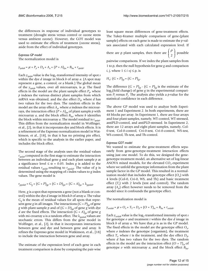
Expresso GP modelThe normalization model is

yspdab = μ + Pp + Dd + Aa + (P × A)pa + Bba + rspdab.

Each yspdab value is the log2-transformed intensity of spot swithin the dye d image in block b of array a. (A spot mayrepresent a gene, a control, or a blank.) The global meanof the yspdab values, over all microarrays, is μ. The fixedeffects in the model are the plant sample effect Pp, wherep indexes the various distinct plant samples from whichmRNA was obtained, and the dye effect Dd, where d hastwo values for the two dyes. The random effects in themodel are the array effect Aa, where a indexes the microar-rays, the interaction effect (P × A)pa of plant sample p withmicroarray a, and the block effect Bba, where b identifiesthe block within microarray a. The model residual is rspdab.This differs from the normalization model in Wolfinger,et al., [2], in that it incorporates dye and block effects. It isa refinement of the Expresso normalization model in Wat-kinson, et al., [18], in that it has no printing pin effect,which is specific to the analysis in the earlier paper, andincludes the block effect.

The second stage of the analysis uses the residual valuesrspdab computed in the first stage to estimate the interactionbetween an individual gene g and each plant sample p ata significance level ≤ α = 0.05. Index g is added to theresidual values rspdab resulting to rgspdab. The value of g isdetermined using the mapping of s index values to g indexvalues. The gene model is

rgspdab = Gg + (G × P)gp + (G × D)gd + (G × A)ga + λgspdab.

Here, g is a spot that represents a gene (not a blank or con-trol) within the dye d image in block b of array a. The valueGg is the mean of residual values for all spots that repre-sent gene g in all images. The interactions (G × P)gp of geneg with plant sample p and of (G × D)gd of gene g with dyed are the fixed effects. The interaction (G × A)ga of gene gwith mi-croarray a is a random effect. The λgspdab values arestochastic errors. This differs from the gene model inWolfinger, et al., [2], in that it incorporates interactionsbetween gene and dye and between gene and array. Itrefines the Expresso gene model in Watkinson, et al., [18]to include the interaction between gene and array.

The estimate of the expression level of each gene in eachtreatment comparison is done by computing the pair-wise

least square mean differences of gene-treatment effects.The Tukey-Kramer multiple comparison of gene-(plantsample) effects on each gene is made to estimate the p val-ues associated with each calculated expression level. If

there are ρ plant samples, then there are possible

pairwise comparisons. If we index the plant samples from

1 to ρ, then the null hypothesis for gene g and comparison

i, j, where 1 ≤ i <j ≤ ρ, is

Ho: (G × P)gi = (G × P)gi.

The difference (G × P)gi - (G × P)gj is the estimate of thelog2(fold change) of gene g in the experimental compari-son Pi versus Pj. The analysis also yields a p-value for thestatistical confidence in each difference.

The above GP model was used to analyze both Experi-ment 1 and Experiment 2. In both experiments, there are48 blocks per array. In Experiment 1, there are four arraysand four plant samples, namely, WT-control, WT-stressed,antiPLD-control, and antiPLD-stressed. In Experiment 2,there are 12 arrays and eight plant samples, namely, Col-0-test, Col-0-control, Cvi-0-test, Cvi-0-control, WS-test,WS-control, Th-test, and Th-control.

Expresso GOT modelWe wanted to estimate the gene-treatment effects sepa-rately from gene-genotype-treatment interaction effectsusing just one model. To do this, we designed the gene-genotype-treatment model, an alternative set of log-linearANOVA mixed models, for the elevated CO2 experimentwhere we unfold the genotype information from the plantsample factor in the GP model. This resulted in a normal-ization model that includes the genotype effect (Oo) with4 levels (Col-0, Cvi-0, WS, and Th) and basic treatmenteffect (Tt) with 2 levels (test and control). The randomarray (Aa) effect however needs to be removed from themodel since it confounds the genotype effect.

The normalization model is

ysotdab = μ + Oo + TT + Dd + (O × T)ot + Bba + rsotdab.

Each ysotdab value is the log2-transformed intensity of spot sfor genotype o and treatment t within the dye d image inblock b of array a. We have that μ is as in the GP model.The fixed effects in the model are the genotype effect Oo,where o indexes the genotype (organism), the treatmenteffect Tt, where t is the treatment, and the dye effect Dd,where d has two values for the two dyes. The randomeffects in the model are the interaction effect (O × T)ot ofgenotype o with microarray a, and the block effect Bba,

ρ2

⎛

⎝⎜

⎞

⎠⎟



where b identifies the block within microarray a. Themodel residual is rsotdab. This differs from the normaliza-tion model in Wolfinger, et al., [2], in that it incorporatesgenotype (organism), dye, and block effects. It is a refine-ment of the Expresso normalization model in Watkinson,et al., [18], in that it has no printing pin effect, andincludes the genotype and block effects.

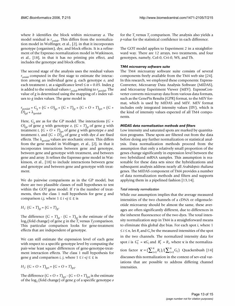
The second stage of the analysis uses the residual valuesrsotdab computed in the first stage to estimate the interac-tion among an individual gene g, each genotype o, andeach treatment t, at a significance level ≤ α = 0.05. Index gis added to the residual values rsotdab resulting to rgsotdab. Thevalue of g is determined using the mapping of s index val-ues to g index values. The gene model is

rgsotdab = Gg + (G × O)go + (G × T)gt + (G × O × T)got + (G ×D)gd + λgsotdab

Here, Gg are as for the GP model. The interactions (G ×O)go of gene g with genotype o, (G × T)gt of gene g withtreatment t, (G × O × T)got of gene g with genotype o andtreatment t, and (G × D)gd of gene g with dye d are fixedeffects. The λgsotdab values are stochastic errors. This differsfrom the gene model in Wolfinger, et al., [2], in that itincorporates interactions between gene and genotype,between gene and genotype with treatment, and betweengene and array. It refines the Expresso gene model in Wat-kinson, et al., [18] to include interactions between geneand genotype and between gene and genotype with treat-ment.

We do pairwise comparisons as in the GP model, butthere are two plausible classes of null hypotheses to testwithin the GOT gene model. If τ is the number of treat-ments, then the class 1 null hypothesis for gene g andcomparison i,j, where 1 ≤ i <j ≤ τ, is

H1: (G × T)gi = (G × T)gj.

The difference (G × T)gi - (G × T)gj is the estimate of thelog2(fold change) of gene g in the Ti versus Tjcomparison.This particular comparison looks for gene-treatmenteffects that are independent of genotype.

We can still estimate the expression level of each genewith respect to a specific genotype level by computing thepair-wise least square differences of gene-genotype-treat-ment interaction effects. The class 1 null hypothesis forgene g and comparison i, j, where 1 ≤ i <j ≤ τ, is

H2: (G × O × T)goi = (G × O × T)goj.

The difference (G × O × T)goi - (G × O × T)goj is the estimateof the log2 (fold change) of gene g of a specific genotype o

for the Ti versus Tj comparison. The analysis also yields ap-value for the statistical confidence in each difference.

The GOT model applies to Experiment 2 in a straightfor-ward way. There are 12 arrays, two treatments, and fourgenotypes, namely, Col-0, Cvi-0, WS, and Th.

TM4 microarray software suiteThe TM4 microarray software suite consists of severalcomponents freely available from the TM4 web site [24].In this research, we employed these components: Express-Converter, Microarray Data Analysis Software (MIDAS),and Microarray Experiment Viewer (MEV). ExpressCon-verter converts microarray data from various data formats,such as the GenePix Results (GPR) format, to the MEV for-mat, which is used by MIDAS and MEV. MEV formatincludes only integrated intensity values (IIV), which isthe kind of intensity values expected of all TM4 compo-nents.

MIDAS data normalization methods and filtersLow intensity and saturated spots are marked by quantita-tion programs. These spots are filtered out from the databefore doing any further normalization or statistical anal-ysis. Data normalization methods proceed from theassumption that only a relatively small proportion of thegenes change significantly in expression level between thetwo hybridized mRNA samples. This assumption is rea-sonable for these data sets since the hybridizations andsubsequent analysis address nearly all Arabidopsis thalianagenes. The MIDAS component of TM4 provides a numberof data normalization methods and filters and supportsapplying them in a pipelined fashion [13,14].

Total intensity normalization

While our assumption implies that the average measuredintensities of the two channels of a cDNA or oligonucle-otide microarray should be almost the same, these aver-ages are often significantly different, due to differences inthe inherent fluorescence of the two dyes. The total inten-sity normalization step in TM4 is a straightforward meansto eliminate this global dye bias. For each spot i, where 1

≤ i ≤ n, let Ri and Gi be the measured intensities of the spot

in the two channels. The normalized intensity data for

spot i is = κGi and = Ri, where κ is the normaliza-

tion factor Quackenbush [14]

discusses this normalization in the context of sev-eral var-iations that are possible to address differing channelintensities.

′Gi ′Ri

κ = = =∑ ∑( )/( )R Giin

iin

1 1



Lowess normalizationBeyond the global dye bias, there is dye bias that isdependent on the measured spot intensities [25,26]. TM4constructs a scatter plot, called an RI-plot, of the points (xi,yi), where 1 ≤ i ≤ n, given by xi = log10(RiGi) and yi =log2(Ri/Gi). Under our assumption, the RI-plot should bevery nearly symmetric with respect to the line y = 0. Inlowess normalization, TM4 applies the lowess method ofCleveland [27] to fit a locally weighted regression curve tothe RI-plot; TM4 then adjusts spot intensities to eliminateany systematic intensity-dependent bias. Additionaldetails on correcting intensity-dependent bias is found in[14].

Standard deviation regularizationAfter total intensity and lowess normalizations eliminatedye bias on a global (per microarray) scale, TM4 employsstandard deviation regularization to ensure that the per-block variances of log(Ri/Gi) values are the same [25,28].Quackenbush [14] provides the formulas for this normal-ization step.

Low intensity filteringSince the relative error in the log(Ri/Gi) values increases ifRi or Gi is close to background levels, spots with low inten-sities are filtered out. Quackenbush [14] provides addi-tional details, which essentially require that both Ri and Giintensities be above two standard deviations of the respec-tive backgrounds.

The MIDAS pipelineWe applied a MIDAS pipeline consisting of total intensitynormalization, lowess normalization, standard deviationregularization, and low intensity filtering to both microar-ray data sets. MIDAS default parameters were usedthroughout; the default low intensity filter cut-off is RiGi <10,000.

TM4 MEV analysisThe Multi Experiment Viewer (MEV) component of TM4provides a number of statistical analyses and clusteringalgorithms to identify differentially expressed genes. Wereport results from the one-class t-test analysis applied tooutput of the MIDAS pipeline. This test assumes that thepaired distribution of treated and control groups is nor-mally distributed. Since the intensities measured from thesame spot are correlated, we can apply the one-class t-testfor the two-group comparison.

Authors' contributionsAAS performed the data preprocessing, Expresso analysisof all data sets, developed the database of statisticalresults, and drafted the manuscript. SPM performed thedrought stress experiment (experiment 1), while PL per-formed the elevated CO2 experiment (experiment 2). PL

performed the qRT-PCR of 192 genes from experiment 2.WS and PL performed TM4 analysis of experiments 1 and2 respectively. LSH supervised the data analysis. LSH, HJB,and RG conceived of the study and coordinated the work.All authors read and approved the manuscript.

Additional material

AcknowledgementsThe work has been supported by the National Science Foundation (DBI-0223905 and BIO/IBN 0219322) and Virginia Tech and UIUC institutional funds.

References1. Churchill GA: Using ANOVA to Analyze Microarray Data. Bio

Techniques 2004, 37(2):173-177.2. Wolfinger R, Gibson G, Wolfinger E, Bennett L, Hamadeh H, Bushel

P, Afshari C, Paules R: Assessing Gene Significance from cDNAMicroarray Expression Data via Mixed Models. Journal of Com-putational Biology 2001, 8:625-637.

3. Kerr MK: Linear Models for Microarray Data Analysis: HiddenSimilarities and Differences. Journal of Computational Biology 2003,10(6):891-901.

4. Pan W: A Comparative Review of Statistical Methods for Dis-covering Differentially Expressed Genes in Replicated Micro-array Experiments. Bioinformatics 2002, 18(4):546-554.

5. Chu TM, Weir B, Wolfinger RD: Comparison of Li-Wong andLoglinear Mixed Models for the Statistical Analysis of Oligo-nucleotide Arrays. Bioinformatics 2004, 20(4):500-506.

6. Cui X, Churchill GA: Statistical Tests for Differential Expres-sion in cDNA Microarray Experiments. Genome Biology 2003,4(210):.

7. Rosa GJ, Steibel JP, Tempelman RJ: Reassessing Design and Anal-ysis of Two-colour Microarray Experiments using MixedEffects Models. Comparative and Functional Genomics 2005,6:123-131.

8. Futschik M, Crompton T: Model Selection and Efficiency Test-ing for Normalization of cDNA Microarray Data. Genome Biol-ogy 2004, 5(R60):.

9. Held M, Gase K, Baldwin IT: Microarray in Ecological Research:A Case Study of a cDNA Microarray for Plant-HerbivoreInteractions. BMS Ecology 2004, 4(13):.

Additional File 1Intensity-dependent dye bias in Rl-plots. Supplementary Figure 1 is a PDF file that contains six RI-plots that illustrate specific intensity-depend-ent dye bias as the microarray data is processed through the normalization steps.Click here for file[http://www.biomedcentral.com/content/supplementary/1471-2105-7-215-S1.pdf]

Additional File 2Genes subjected to qRT-PCR. Supplementary Table 1 is a PDF file that contains the annotation of genes subjected to qRT-PCR and the functional categories represented. For verification of microarray results in Experi-ment 2, Li, et al., [23] performed real-time quantitative reverse-tran-scriptase PCR (qRT-PCR) for selected genes — 55 in Col-0; 52 in Cvi-0; 59 in WS; 26 in Th. The AT numbers of those genes, their annotation, and categorizations into biological functions are in the table.Click here for file[http://www.biomedcentral.com/content/supplementary/1471-2105-7-215-S2.pdf]


http://www.biomedcentral.com/content/supplementary/1471-2105-7-215-S1.pdf

http://www.biomedcentral.com/content/supplementary/1471-2105-7-215-S2.pdf
















Publish with BioMed Central and every scientist can read your work free of charge

"BioMed Central will be the most significant development for disseminating the results of biomedical research in our lifetime."

Sir Paul Nurse, Cancer Research UK

Your research papers will be:

available free of charge to the entire biomedical community

peer reviewed and published immediately upon acceptance

cited in PubMed and archived on PubMed Central

yours — you keep the copyright

Submit your manuscript here:http://www.biomedcentral.com/info/publishing_adv.asp

BioMedcentral

10. Xie Y, Jeong KS, Pan W, Khodursky A, Carlin BP: A Case Study onChoosing Normalization Methods and Test Statistics forTwo-Channel Microarray Data. Comparative and FunctionalGenomics 2004, 5:432-444.

11. Bolstad B, Irizarry R, Astrand M, Speed T: A Comparison of Nor-malization Methods for High Density Oligonucleotide ArrayData Based on Variance and Bias. Bioinformatics 2003,19(2):185-193.

12. Dudoit S, Gentleman RC, Quackenbush J: Open Source Softwarefor the Analysis of Microarray Data. BioTechniques 2003,34:s45-s51.

13. Saeed A, Sharov V, White J, Li J, Liang W, Bhagabati N, Braisted J,Klapa M, Currier T, Thiagarajan M, Sturn A, Snuffin M, Rezantsev A,Popov D, Ryltsov A, Kostukovich E, Borisovsky I, Liu Z, Vinsavich A,Trush V, Quackenbush J: TM4: A Free, Open-Source System forMicroarray Data Management and Analysis. Bio Techniques2003, 34:374-378.

14. Quackenbush J: Microarray Data Normalization and Transfor-mation. Nature Genetics Supplement 2002, 32:496-501.

15. Williams RD, King SN, Greer BT, Whiteford CC, Wei JS, Natrajan R,Kelsey A, Rogers S, Campbell C, Pritchard-Jones K, Khan J: Prognos-tic Classification of Relapsing Favorable Histology WilmsTumor using cDNA Microarray Expression Profiling andSupport Vector Machines. Genes, Chromosomes and Cancer 2004,41:65-79.

16. Zhu X, Hart R, Chang MS, Kim JW, Lee SY, Cao YA, Mock D, Ke E,Saunders B, Alexander A, Grossoehme J, Lin KM, Yan Z, Hsueh R, LeeJ, Scheuermann RH, Fruman DA, Seaman W, Subramaniam S, Stern-weis P, Simon MI, Choi S: Analysis of the Major Patterns of BCell Gene Expression Changes in Response to Short-TermStimulation with 33 Single Ligands. The Journal of Immunology2004, 173:7141-7149.

17. Khaitovich P, Weiss G, Lachmann M, Hellmann I, Enard W, MuetzelB, Wirkner U, Ansorge W, Paabo S: A Neutral Model of Tran-scriptome Evolution. PLoS Biology 2004, 2(5):682-689.

18. Watkinson JI, Sioson AA, Vasquez-Robinet C, Shukla M, Kumar D,Ellis M, Heath LS, Ramakrishnan N, Chevone B, Watson LT, van ZylL, Egertsdotter U, Sederoff RR, Grene R: Photosynthetic Acclima-tion is Reflected in Specific Patterns of Gene Expression inDrought-Stressed Loblolly Pine. Plant Physiology 2003,133(4):1702-1716.

19. Sioson AA, Watkinson JI, Vasquez-Robinet C, Ellis M, Shukla M,Kumar D, Ramakrishnan N, Heath LS, Grene R, Chevone BI, KadafarK, Watson LT: Expresso and Chips: Creating a Next Genera-tion Microarray Experiment Management System. In Proceed-ings of the Next Generation Software Systems Workshop, 17thInternational Parallel and Distributed Processing Symposium (IPDPS '03)Nice, France; 2003:209b.

20. Heath LS, Ramakrishnan N, Sederoff RR, Whetten RW, Chevone BI,Struble CA, Jouenne VY, Chen D, van Zyl LM, Grene R: Studyingthe Functional Genomics of Stress Responses in LoblollyPine using the Expresso Microarray Management System.Comparative and Functional Genomics 2002, 3:226-243.

21. Galbraith D: Arabidopsis Oligonucleotide Microarrays. [http://www.ag.arizona.edu/microarray/].

22. Mane SP, Vasquez-Robinet C, Sioson AA, Heath LS, Grene R: Phos-pholipase D alpha is Involved in Drought Stress Signaling inArabidopsis. Poster presented at the International Conference on PlantLipid-Mediated Signaling, Raleigh, NC 2005.

23. Li P, Sioson AA, Mane SP, Ulanov A, Grothaus G, Heath LS, MuraliTM, Bohnert HJ, Grene R: Response Diversity of Arabidopsisthaliana Ecotypes and Thellungiella halophila in elevated CO2in the field. Manuscript submitted 2005.

24. TM4 [http://www.tm4.org/]25. Yang YH, Dudoit S, Luu P, Lin DM, Peng V, Ngai J, Speed TP: Nor-

malization for cDNA Microarray Data: A Robust CompositeMethod Addressing Single and Multiple Slide SystematicVariation. Nucleic Acids Research 2002, 30(4):e15.

26. Yang I, Chen E, Hasseman J, Liang W, Frank B, Wang S, Sharov V,Saeed A, White J, Li J, Lee N, Yeatman T, Quackenbush J: Within theFold: Assessing Differential Expression Measures and Repro-ducibility in Microarray Assays. Genome Biology 2002,3(11):1-12.

27. Cleveland W: Robust Locally Weighted Regression andSmoothing Scatterplots. J Amer Stat Assoc 1979, 74:829-836.

28. Huber W, von Heydebreck A, Sultmann H, Poustka A, Vingron M:Variance Stabilization Applied to Microarray Data Calibra-tion and to the Quantification of Differential Expression. Bio-informatics 2002, 18(Suppl 1):S96-S104.











http://www.ag.arizona.edu/microarray/

http://www.ag.arizona.edu/microarray/

http://www.tm4.org/








http://www.biomedcentral.com/info/publishing_adv.asp


bmc bioinformatics biomed central bioinformatics research article open access the statistics of...

Documents