arX

iv:h

ep-p

h/04

0931

7v2

9 D

ec 2

004

BNL-HET-04/17

December, 2004

Final State Interactions in Hadronic B Decays

Hai-Yang Cheng,1 Chun-Khiang Chua1 and Amarjit Soni2

1 Institute of Physics, Academia Sinica

Taipei, Taiwan 115, Republic of China

2 Physics Department, Brookhaven National Laboratory

Upton, New York 11973

Abstract

There exist many experimental indications that final-state interactions (FSIs) may play a promi-

nent role not only in charmful B decays but also in charmless B ones. We examine the final-state

rescattering effects on the hadronic B decay rates and their impact on direct CP violation. The

color-suppressed neutral modes such as B0 → D0π0, π0π0, ρ0π0,K0π0 can be substantially en-

hanced by long-distance rescattering effects. The direct CP -violating partial rate asymmetries in

charmless B decays to ππ/πK and ρπ are significantly affected by final-state rescattering and their

signs are generally different from that predicted by the short-distance approach. For example, di-

rect CP asymmetry in B0 → ρ0π0 is increased to around 60% due to final state rescattering effects

whereas the short-distance picture gives about 1%. Evidence of direct CP violation in the decay

B0 → K−π+ is now established, while the combined BaBar and Belle measurements of B

0 → ρ±π∓

imply a 3.6σ direct CP asymmetry in the ρ+π− mode. Our predictions for CP violation agree

with experiment in both magnitude and sign, whereas the QCD factorization predictions (espe-

cially for ρ+π−) seem to have some difficulty with the data. Direct CP violation in the decay

B− → π−π0 is very small ( <∼ 1%) in the Standard Model even after the inclusion of FSIs. Its

measurement will provide a nice way to search for New Physics as in the Standard Model QCD

penguins cannot contribute (except by isospin violation). Current data on πK modes seem to

violate the isospin sum rule relation, suggesting the presence of electroweak penguin contributions.

We have also investigated whether a large transverse polarization in B → φK∗ can arise from the

final-state rescattering of D(∗)D(∗)s into φK∗. While the longitudinal polarization fraction can be

reduced significantly from short-distance predictions due to such FSI effects, no sizable perpen-

dicular polarization is found owing mainly to the large cancellations occurring in the processes

B → D∗sD → φK

∗and B → DsD

∗ → φK∗and this can be understood as a consequence of

CP and SU(3) [CPS] symmetry. To fully account for the polarization anomaly (especially the

perpendicular polarization) observed in B → φK∗, FSI from other states or other mechanism, e.g.

the penguin-induced annihilation, may have to be invoked. Our conclusion is that the small value

of the longitudinal polarization in V V modes cannot be regarded as a clean signal for New Physics.

1

I. INTRODUCTION

The importance of final-state interactions (FSIs) has long been recognized in hadronic charm

decays since some resonances are known to exist at energies close to the mass of the charmed

meson. As for hadronic B decays, the general folklore is that FSIs are expected to play only a

minor role there as the energy release in the energetic B decay is so large that the final-state

particles are moving fast and hence they do not have adequate time for getting involved in final-

state rescattering. However, from the data accumulated at B factories and at CLEO, there are

growing indications that soft final-state rescattering effects do play an essential role in B physics.

Some possible hints at FSIs in the B sector are:

1. There exist some decays that do not receive any factorizable contributions, for example B →Kχ0c, owing to the vanishing matrix element of the (V −A) current, 〈χ0c|cγµ(1−γ5)c|0〉 = 0.

Experimentally, it was reported by both Belle [1] and BaBar [2] that this decay mode has

a sizable branching ratio, of order (2 ∼ 6) × 10−4. This implies that the nonfactorizable

correction is important and/or the rescattering effect is sizable. Studies based on the light-

cone sum rule approach indicate that nonfactorizable contributions to B → χc0K due to soft

gluon exchanges is too small to accommodate the data [3, 4]. In contrast, it has been shown

that the rescattering effect from the intermediate charmed mesons is able to reproduce the

observed large branching ratio [5].

2. The color-suppressed modes B0 → D(∗)0π0 have been measured by Belle [6], CLEO [7] and

BaBar [8]. Their branching ratios are all significantly larger than theoretical expectations

based on naive factorization. When combined with the color-allowed B → D(∗)π decays, it

indicates non-vanishing relative strong phases among various B → D(∗)π decay amplitudes.

Denoting T and C as the color-allowed tree amplitude and color-suppressed W -emission

amplitude, respectively, it is found that C/T ∼ 0.45 exp(±i60◦) (see e.g. [9]), showing a

non-trivial relative strong phase between C and T amplitudes. The large magnitude and

phase of C/T compared to naive expectation implies the importance of long-distance FSI

contributions to the color-suppressed internal W -emission via final-state rescattering of the

color-allowed tree amplitude.

3. A model independent analysis of charmless B decay data based on the topological quark

diagrammatic approach yields a larger value of |C/T | and a large strong relative phase

between the C and T amplitudes [10]. For example, one of the fits in [10] leads to

C/T = (0.46+0.43−0.30) exp([−i(94+43

−52)]◦, which is indeed consistent with the result inferred from

B → Dπ decays. This means that FSIs in charmless B decays are as important as in B → Dπ

ones. The presence of a large color-suppressed amplitude is somewhat a surprise from the

current model calculations such as those in the QCD factorization approach and most likely

indicates a prominent role for final-state rescattering.

4. Both BaBar [11] and Belle [12] have reported a sizable branching ratio of order 2× 10−6 for

the decay B0 → π0π0. This cannot be explained by either QCD factorization or the PQCD

2

approach and it again calls for a possible rescattering effect to induce π0π0. Likewise, the

color-suppressed decay B0 → ρ0π0 with the branching ratio (1.9± 1.2)× 10−6 averaged from

the Belle and BaBar measurements (see Table V) is substantially higher than the prediction

based on PQCD [13] or the short-distance approach. Clearly, FSI is one of the prominent

candidates responsible for this huge enhancement.

5. Direct CP violation in the decay B0 → K+π− with the magnitude AKπ = −0.133± 0.030±0.009 at 4.2σ was recently announced by BaBar [14], which agrees with the previous Belle

measurement of AKπ = −0.088± 0.035± 0.013 at 2.4σ based on a 140 fb−1 data sample [15].

A further evidence of this direct CP violation at 3.9σ was just reported by Belle with 253 fb−1

of data [16]. In the calculation of QCD factorization [17, 18], the predicted CP asymmetry

AKπ = (4.5+9.1−9.9)% is apparently in conflict with experiment. It is conceivable that FSIs via

rescattering will modify the prediction based on the short-distance interactions. Likewise,

a large direct CP asymmetry in the decay B0 → π+π− was reported by Belle [19], but

it has not been confirmed by BaBar [20]. The weighted average of Belle and BaBar gives

Aππ = 0.31± 0.24 [21] with the PDG scale factor of S = 2.2 on the error. Again, the central

value of the QCD factorization prediction [18] has a sign opposite to the world average.

6. Under the factorization approach, the color-suppressed mode B0 → D+

s K− can only proceed

viaW -exchange. Its sizable branching ratio of order 4×10−5 observed by Belle [22] and BaBar

[23] will need a large final-state rescattering contribution if the short-distance W -exchange

effect is indeed small according to the existing model calculations.

7. The measured longitudinal fractions for B → φK∗ by both BaBar [24] and Belle [25] are close

to 50%. This is in sharp contrast to the general argument that factorizable amplitudes in B

decays to light vector meson pairs give a longitudinal polarization satisfying the scaling law:

1 − fL = O(1/m2b ).

1 This law remains formally true even when nonfactorizable graphs are

included in QCD factorization. Therefore, in order to obtain a large transverse polarization

in B → φK∗, this scaling law valid at short-distance interactions must be violated. The

effect of long-distance rescattering on this scaling law should be examined.

The presence of FSIs can have interesting impact on the direct CP violation phenomenology.

As stressed in [28], traditional discussions have centered around the absorptive part of the penguin

graph in b → s transitions [29] and as a result causes “simple” CP violation; long-distance final

state rescattering effects, in general, will lead to a different pattern of CP violation, namely,

“compound” CP violation. Predictions of simple CP violation are quite distinct from that of

compound CP violation. The sizable CP asymmetry observed in B0 → K−π+ decays is a strong

indication for large direct CP violation driven by long-distance rescattering effects. Final state

1 More recently Kagan has suggested that the penguin-induced annihilation can cause an appreciable devia-

tion from this expectation numerically, though the scaling law is still respected formally [26, 27]. However,

it is difficult to make a reliable estimation of this deviation.

3

rescattering phases in B decays are unlikely to be small possibly causing large compound CP -

violating partial rate asymmetries in these modes. As shown below, the sign of CP asymmetry

can be easily flipped by long-distance rescattering effects. Hence, it is important to explore the

compound CP violation.

Of course, it is notoriously difficult to study FSI effects in a systematic way as it is nonperturba-

tive in nature. Nevertheless, we can gain some control on rescattering effects by studying them in

a phenomenological way. More specifically, FSIs can be modelled as the soft rescattering of certain

intermediate two-body hadronic channels, e.g. B → DD → ππ, so that they can be treated as the

one-particle-exchange processes at the hadron level. That is, we shall study long-distance rescatter-

ing effects by considering one-particle-exchange graphs. As the exchanged particle is not on-shell,

form factors must be introduced to render the whole calculation meaningful in the perturbative

sense. This approach has been applied to the study of FSIs in charm decays for some time [30, 31].

In the context of B physics, the so-called “charming penguin” contributions to charmless hadronic

B decays have been treated as long-distance effects manifesting in the rescattering processes such

as B → DsD → Kπ [32, 33, 34]. Likewise, the dynamics for final-state interactions is assumed to

be dominated by the mixing of the final state with D(∗)D(∗) in [35, 36]. Final-state rescattering

effects were also found in B to charmonium final states, e.g. B− → K−χc0, a process prohibited in

the naive factorization approach [5]. Effects of final-state rescattering on Kπ and ππ final states

have been discussed extensively in the literature [28, 37, 38].

The approach of modelling FSIs as soft rescattering processes of intermediate two-body states

has been criticized on several grounds [39]. First, there are many more intermediate multi-body

channels in B decays and systematic cancellations among them are predicted to occur in the heavy

quark limit. This effect of cancellation will be missed if only a few intermediate states are taken

into account. Second, the hadronic dynamics of multi-body decays is very complicated and in

general not under theoretical control. Moreover, the number of channels and the energy release

in B decays are large. We wish to stress that the b quark mass (∼ 4.5 GeV) is not very large

and far from infinity in reality. The aforementioned cancellation may not occur or may not be

very effective for the finite B mass. For intermediate two-body states, we always consider those

channels that are quark-mixing-angle most favored so that they give the dominant long-distance

contributions. Whether there exist cancellations between two-body and multi-body channels is not

known. Following [40], we may assume that two-body ⇀↽ n-body rescatterings are negligible either

justified from the 1/Nc argument [41] or suppressed by large cancellations. We view our treatment

of the two-body hadronic model for FSIs as a working tool. We work out the consequences of

this tool to see if it is empirically working. If it turns out to be successful, then it will imply

the possible dominance of intermediate two-body contributions. In other approaches such as QCD

factorization [17], the complicated hadronic B decays in principle can be treated systematically

as 1/mb power corrections which vanish in the heavy quark limit. However, one should recognize

that unless the coefficients of power corrections are known or calculable in a model independent

manner, the short-distance picture without a control of the 1/mb coefficients and without being

able to include the effects of FSIs have their limitation as well. When the short-distance scenario is

tested against experiment and failings occur such as the many examples mentioned before, then it

4

does not necessarily mean that New Physics has been discovered and an examination of rescattering

effects can be helpful.

The layout of the present paper is as follows. In Sec. II we give an overview of the role played by

the final-state interactions in hadronic B decays. As a warm-up, we begin in Sec. III with a study of

final-state rescattering contributions to B → Dπ decays which proceed only through tree diagrams.

We then proceed to the penguin-dominated B → Kπ decays in Sec. IV, tree-dominated B → ππ

decays in Sec. V and B → ρπ decays in Sec. VI. Effects of FSIs on the branching ratios and direct

CP asymmetries are studied. Sec. VII is devoted to the polarization anomaly discovered recently

in B → φK∗ decays. Conclusion and discussion are given in Sec. VIII. Appendix A gives some

useful formula for the phase-space integration, while the theoretical input parameters employed in

the present paper are summarized in Appendix B.

II. FINAL-STATE INTERACTIONS

In the diagrammatic approach, all two-body nonleptonic weak decays of heavy mesons can be

expressed in terms of six distinct quark diagrams [42, 43, 44]: T , the color-allowed external W -

emission tree diagram; C, the color-suppressed internal W -emission diagram; E , the W -exchange

diagram; A, the W -annihilation diagram; P, the penguin diagram; and V, the vertical W -loop

diagram. It should be stressed that these quark diagrams are classified according to the topologies

of weak interactions with all strong interaction effects included and hence they are not Feynman

graphs. All quark graphs used in this approach are topological with all the strong interactions

included, i.e. gluon lines are included in all possible ways.

As stressed above, topological graphs can provide information on final-state interactions (FSIs).

In general, there are several different forms of FSIs: elastic scattering and inelastic scattering such

as quark exchange, resonance formation,· · ·, etc. Take the decay B0 → D0π0 as an illustration.

The topological amplitudes C, E , A can receive contributions from the tree amplitude T of e.g.

B0 → D+π− via final-state rescattering, as illustrated in Fig. 1: Fig. 1(a) has the same topology as

W -exchange, while 1(b) and 1(c) mimic the internalW -emission amplitude C. Therefore, even if the

short-distanceW -exchange vanishes, a long-distanceW -exchange can be induced via inelastic FSIs.

Historically, it was first pointed out in [45] that rescattering effects required by unitarity can produce

the reaction D0 → K0φ, for example, even in the absence of the W -exchange diagram. Then it

was shown in [42] that this rescattering diagram belongs to the generic W -exchange topology.

Since FSIs are nonperturbative in nature, in principle it is extremely difficult to calculate their

effects. It is customary to evaluate the long-distance W -exchange contribution, Fig. 1(a), at the

hadron level manifested as Fig. 2 [30, 31, 46]. Fig. 2(a) shows the resonant amplitude coming

from B0 → D+π− followed by a s-channel JP = 0+ particle exchange with the quark content (cu),

which couples to D0π0 and D+π−. Fig. 2(b) corresponds to the t-channel contribution with a

ρ particle exchange. The relative phase between T and C indicates some final-state interactions

responsible for this. Figs. 1(b) and 1(c) show that final-state rescattering via quark exchange has

the same topology as the color-suppressed internal W -emission amplitude. At the hadron level,

5

cd

B0

D+

π−

D0

u

π0

u

cb

dud

(a)

cd

B0

D+

π−

d

D0

u

d

π0

d

b c

u

(b)

dd

B0

D+

π−

c

π0

d

u

D0

u

cb

d

(c)

FIG. 1: Contributions to B0 → D0π0 from the color-allowed weak decay B

0 → D+π− followed by

a resonant-like rescattering (a) and quark exchange (b) and (c). While (a) has the same topology

as the W -exchange graph, (b) and (c) mimic the color-suppressed internal W -emission graph.

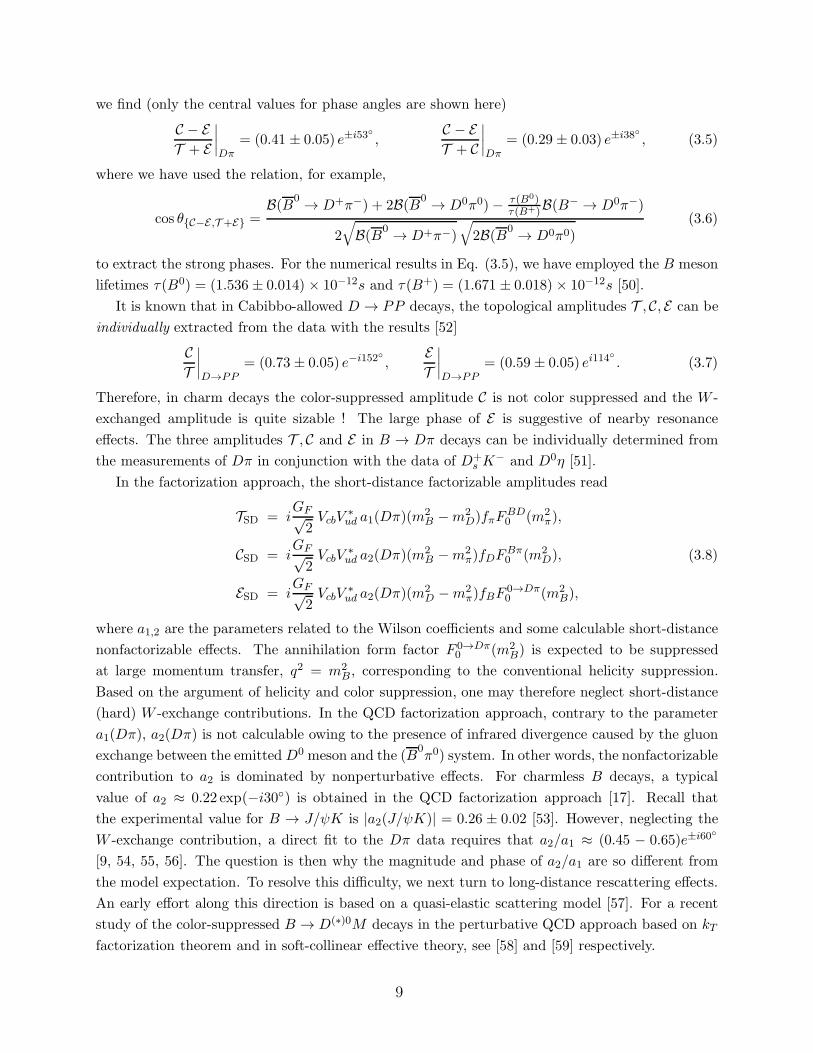
Figs. 1(b) and 1(c) are manifested in the rescattering processes with one particle exchange in the

t channel [30] (see Fig. 3). Note that Figs. 3(a) and 2(b) are the same at the meson level even

though at the quark level they correspond to different processes, namely, annihilation and quark

exchange, respectively. In contrast, Fig. 3(b) is different than Fig. 3(a) in the context of the

t-channel exchanged particle.

For charm decays, it is expected that the long-distance W -exchange is dominated by resonant

FSIs as shown in Fig. 2(a). That is, the resonance formation of FSI via qq resonances is probably

the most important one due to the fact that an abundant spectrum of resonances is known to exist

at energies close to the mass of the charmed meson. However, a direct calculation of this diagram

6

✧✦★✥

✲

✲

��✒

��

❅❅❘

❅❅

B0

π−

D+

π0

D0

(a)

��✒

��

❅❅❘

❅❅

❄

✲

✲

B0

π−

D+

ρ+

π0

D0

(b)

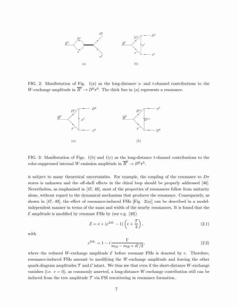
FIG. 2: Manifestation of Fig. 1(a) as the long-distance s- and t-channel contributions to the

W -exchange amplitude in B0 → D0π0. The thick line in (a) represents a resonance.

��✒

��

❅❅❘

❅❅

❄

✲

✲

B0

π−

D+

ρ+

π0

D0

(a)

��✒

��

❅❅❘

❅❅

❄

✲

✲

B0

π−

D+

D∗+

D0

π0

(b)

FIG. 3: Manifestation of Figs. 1(b) and 1(c) as the long-distance t-channel contributions to the

color-suppressed internal W -emission amplitude in B0 → D0π0.

is subject to many theoretical uncertainties. For example, the coupling of the resonance to Dπ

states is unknown and the off-shell effects in the chiral loop should be properly addressed [46].

Nevertheless, as emphasized in [47, 48], most of the properties of resonances follow from unitarity

alone, without regard to the dynamical mechanism that produces the resonance. Consequently, as

shown in [47, 49], the effect of resonance-induced FSIs [Fig. 2(a)] can be described in a model-

independent manner in terms of the mass and width of the nearby resonances. It is found that the

E amplitude is modified by resonant FSIs by (see e.g. [49])

E = e+ (e2iδr − 1)

(

e+T3

)

, (2.1)

with

e2iδr = 1− iΓ

mD −mR + iΓ/2, (2.2)

where the reduced W -exchange amplitude E before resonant FSIs is denoted by e. Therefore,

resonance-induced FSIs amount to modifying the W -exchange amplitude and leaving the other

quark-diagram amplitudes T and C intact. We thus see that even if the short-distance W -exchange

vanishes (i.e. e = 0), as commonly asserted, a long-distance W -exchange contribution still can be

induced from the tree amplitude T via FSI rescattering in resonance formation.

7

In B decays, in contrast to D decays, the resonant FSIs will be expected to be suppressed

relative to the rescattering effect arising from quark exchange owing to the lack of the existence of

resonances at energies close to the B meson mass. This means that one can neglect the s-channel

contribution from Fig. 2(a).

As stressed before, the calculation of the meson level Feynman diagrams in Fig. 2 or Fig.

3 involves many theoretical uncertainties. If one naively calculates the diagram, one obtains an

answer which does not make sense in the context of perturbation theory since the contributions

become so large that perturbation theory is no longer trustworthy. For example, consider the loop

contribution to B0 → π+π− via the rescattering process D+D− → π+π−. Since B0 → π+π− is

CKM suppressed relative to B0 → D+D−, the loop contribution is larger than the initial B → ππ

amplitude. Because the t-channel exchanged particle is not on-shell, as we shall see later, a form-

factor cutoff must be introduced to the vertex to render the whole calculation meaningful.

III. B → Dπ DECAYS

The color-suppressed decays of B0into D(∗)0π0,D0η,D0ω and D0ρ0 have been observed by

Belle [6] and B0decays into D(∗)0π0 have been measured by CLEO [7]. Recently, BaBar [8]

has presented the measurements of B0decays into D(∗)0(π0, η, ω) and D0η′. All measured color-

suppressed decays have similar branching ratios with central values between 1.7 × 10−4 and 4.2 ×10−4. They are all significantly larger than theoretical expectations based on naive factorization.

For example, the measurement B(B0 → D0π0) = 2.5×10−4 (see below) is larger than the theoretical

prediction, (0.58 ∼ 1.13)× 10−4 [9], by a factor of 2 ∼ 4. Moreover, the three B → Dπ amplitudes

form a non-flat triangle, indicating nontrivial relative strong phases between them. In this section

we will focus on B → Dπ decays and illustrate the importance of final-state rescattering effects.

In terms of the quark-diagram topologies T , C and E , where T is the color-allowed external

W -emission tree amplitude, C, E are color-suppressed internal W -emission and W -exchange am-

plitudes, respectively, the B → Dπ amplitudes can be expressed as

A(B0 → D+π−) = T + E ,

A(B− → D0π−) = T + C, (3.1)

A(B0 → D0π0) =

1√2(−C + E),

and they satisfy the isospin triangle relation

A(B0 → D+π−) =

√2A(B

0 → D0π0) +A(B− → D0π−). (3.2)

Using the data [50]

B(B0 → D+π−) = (2.76 ± 0.25) × 10−3,

B(B− → D0π−) = (4.98 ± 0.29) × 10−3, (3.3)

and the world average B(B0 → D0π0) = (2.5 ± 0.2)× 10−4 from the measurements

B(B0 → D0π0) =

(2.9 ± 0.2 ± 0.3)× 10−4, BaBar [8]

(2.31 ± 0.12 ± 0.23) × 10−4, Belle [6]

(2.74+0.36−0.32 ± 0.55) × 10−4, CLEO [7]

(3.4)

8

we find (only the central values for phase angles are shown here)

C − ET + E

∣

∣

∣

∣

Dπ= (0.41 ± 0.05) e±i53

◦

,C − ET + C

∣

∣

∣

∣

Dπ= (0.29 ± 0.03) e±i38

◦

, (3.5)

where we have used the relation, for example,

cos θ{C−E,T +E} =B(B0 → D+π−) + 2B(B0 → D0π0)− τ(B0)

τ(B+)B(B− → D0π−)

2√

B(B0 → D+π−)√

2B(B0 → D0π0)(3.6)

to extract the strong phases. For the numerical results in Eq. (3.5), we have employed the B meson

lifetimes τ(B0) = (1.536 ± 0.014) × 10−12s and τ(B+) = (1.671 ± 0.018) × 10−12s [50].

It is known that in Cabibbo-allowed D → PP decays, the topological amplitudes T , C, E can be

individually extracted from the data with the results [52]

CT

∣

∣

∣

∣

D→PP= (0.73 ± 0.05) e−i152

◦

,ET

∣

∣

∣

∣

D→PP= (0.59 ± 0.05) ei114

◦

. (3.7)

Therefore, in charm decays the color-suppressed amplitude C is not color suppressed and the W -

exchanged amplitude is quite sizable ! The large phase of E is suggestive of nearby resonance

effects. The three amplitudes T , C and E in B → Dπ decays can be individually determined from

the measurements of Dπ in conjunction with the data of D+s K

− and D0η [51].

In the factorization approach, the short-distance factorizable amplitudes read

TSD = iGF√2VcbV

∗ud a1(Dπ)(m

2B −m2

D)fπFBD0 (m2

π),

CSD = iGF√2VcbV

∗ud a2(Dπ)(m

2B −m2

π)fDFBπ0 (m2

D), (3.8)

ESD = iGF√2VcbV

∗ud a2(Dπ)(m

2D −m2

π)fBF0→Dπ0 (m2

B),

where a1,2 are the parameters related to the Wilson coefficients and some calculable short-distance

nonfactorizable effects. The annihilation form factor F 0→Dπ0 (m2

B) is expected to be suppressed

at large momentum transfer, q2 = m2B , corresponding to the conventional helicity suppression.

Based on the argument of helicity and color suppression, one may therefore neglect short-distance

(hard) W -exchange contributions. In the QCD factorization approach, contrary to the parameter

a1(Dπ), a2(Dπ) is not calculable owing to the presence of infrared divergence caused by the gluon

exchange between the emittedD0 meson and the (B0π0) system. In other words, the nonfactorizable

contribution to a2 is dominated by nonperturbative effects. For charmless B decays, a typical

value of a2 ≈ 0.22 exp(−i30◦) is obtained in the QCD factorization approach [17]. Recall that

the experimental value for B → J/ψK is |a2(J/ψK)| = 0.26 ± 0.02 [53]. However, neglecting the

W -exchange contribution, a direct fit to the Dπ data requires that a2/a1 ≈ (0.45 − 0.65)e±i60◦

[9, 54, 55, 56]. The question is then why the magnitude and phase of a2/a1 are so different from

the model expectation. To resolve this difficulty, we next turn to long-distance rescattering effects.

An early effort along this direction is based on a quasi-elastic scattering model [57]. For a recent

study of the color-suppressed B → D(∗)0M decays in the perturbative QCD approach based on kT

factorization theorem and in soft-collinear effective theory, see [58] and [59] respectively.

9

��✒

��

❅❅❘

❅❅

❄

✲

✲

B

π

D

ρ

π

D

(a)

��✒

��

❅❅❘

❅❅

❄

✲

✲

B

π

D

D∗

D

π

(b)

��✒

��

❅❅❘

❅❅

❄

✲

✲

B

ρ

D∗

π

π

D

(c)

��✒

��

❅❅❘

❅❅

❄

✲

✲

B

ρ

D∗

D

D

π

(d)

��✒

��

❅❅❘

❅❅

❄

✲

✲

B

ρ

D∗

D∗

D

π

(e)

��✒

��

❅❅❘

❅❅

❄

✲

✲

B

a1

D∗

ρ

π

D

(f)

FIG. 4: Long-distance t-channel rescattering contributions to B → Dπ.

A. Long-distance contributions to B → Dπ

Some possible leading long-distance FSI contributions to B → Dπ are depicted in Fig. 4. Apart

from the Dπ intermediate state contributions as shown in Figs. 2 and 3, here we have also included

rescattering contributions from the D∗ρ and D∗a1 intermediate states. As noted in passing, the

s-channel contribution is presumably negligible owing to the absence of nearby resonances. Hence,

we will focus only on the t-channel long-distance contributions. For each diagram in Fig. 4, one

should consider all the possible isospin structure and draw all the possible sub-diagrams at the

quark level [31]. While all the six diagrams contribute to B− → D0π−, only the diagrams 4(a),

4(c) and 4(f) contribute to B0 → D+π− and 4(b), 4(d) and 4(e) to B

0 → D0π0. To see this, we

consider the contribution of Fig. 4(a) to B0 → D0π0 as an example. The corresponding diagrams

of Fig. 4(a) at the quark level are Figs. 1(a) and 1(b). At the meson level, Fig. 4(a) contains

Figs. 2(b) and 3(a). Owing to the wave function π0 = (uu − dd)/√2, Fig. 1(a) and hence Fig.

2(b) has an isospin factor of 1/√2, while Fig. 1(b) and hence Fig. 3(a) has a factor of −1/

√2.

Consequently, there is a cancellation between Figs. 2(b) and 3(a). Another way for understanding

this cancellation is to note that Fig. 2(b) contributes to E , while Fig. 3(a) to C. From Eq. (3.1),

it is clear that there is a cancellation between them.

Given the weak Hamiltonian in the form HW =∑

i λiQi, where λi is the combination of the

quark mixing matrix elements and Qi is a T -even local operator (T : time reversal), the absorptive

part of Fig. 4 can be obtained by using the optical theorem and time-reversal invariant weak decay

operator Qi. From the time reversal invariance of Q (= UTQ∗U †

T ), it follows that

〈i; out|Q|B; in〉∗ =∑

j

S∗ji〈j; out|Q|B; in〉, (3.9)

where Sij ≡ 〈i; out| j; in〉 is the strong interaction S-matrix element, and we have used

10

UT |out (in)〉∗ = |in (out)〉 to fix the phase convention.2 Eq. (3.9) implies an identity related to

the optical theorem. Noting that S = 1 + iT , we find

2Abs 〈i; out|Q|B; in〉 =∑

j

T ∗ji〈j; out|Q|B; in〉, (3.10)

where use of the unitarity of the S-matrix has been made. Specifically, for two-body B decays, we

have

AbsM(pB → p1p2) =1

2

∑

j

(

Πjk=1

∫

d3~qk(2π)32Ek

)

(2π)4

× δ4(p1 + p2 −j∑

k=1

qk)M(pB → {qk})T ∗(p1p2 → {qk}). (3.11)

Thus the optical theorem relates the absorptive part of the two-body decay amplitude to the sum

over all possible B decay final states {qk}, followed by strong {qk} → p1p2 rescattering.

Neglecting the dispersive parts for the moment, the FSI corrections to the topological amplitudes

are

T = TSD,C = CSD + iAbs (4a+ 4b+ 4c+ 4d+ 4e+ 4f), (3.12)

E = ESD + iAbs (4a+ 4c+ 4f).

The color-allowed amplitude T does receive contributions from, for example, the s-channel B0 →

D+π− → D+π− and the t-channel rescattering process B0 → D0π0 → D+π−. However, they

are both suppressed: The first one is subject to O(1/m2b) suppression while the weak decay in the

second process is color suppressed. Therefore, it is safe to neglect long-distance corrections to T .

As a result,

A(B0 → D+π−) = TSD + ESD + iAbs (4a+ 4c+ 4f),

A(B− → D0π−) = TSD + CSD + iAbs (4a+ 4b+ 4c+ 4d+ 4e+ 4f), (3.13)

A(B0 → D0π0) =

1√2(−C + E)SD − i√

2Abs (4b+ 4d+ 4e).

Note that the isospin relation (3.2) is still respected, as it should be.

To proceed we write down the relevant Lagrangian [60, 61]3

L = −igρππ(

ρ+µ π0↔∂ µπ− + ρ−µ π

+↔∂ µπ0 + ρ0µπ

− ↔∂ µπ+

)

2 Note that in the usual phase convention we have T |P (~p)〉 = −|P (−~p)〉, T |V (~p, λ)〉 = −(−)λ|V (−~p, λ)〉with λ being the helicity of the vector meson. For the B → PP, V P, V V decays followed by two-particle

to two-particle rescatterings, the |PP 〉 and S,D-wave |V V 〉 states satisfy the UT |out (in)〉∗ = |in (out)〉relation readily, while for |B〉 and P -wave |V V 〉 as well as |V P 〉 states we may assign them an additional

phase i to satisfy the above relation. We shall return to the usual phase convention once the optical

theorem for final-state rescattering, namely, Eq. (3.10), is obtained.3 In the chiral and heavy quark limits, the effective Lagrangian of (3.15) can be recast compactly in terms

11

− igD∗DP (Di∂µPijD

∗j†µ −D∗i

µ ∂µPijD

j†) +1

2gD∗D∗P εµναβ D

∗µi ∂

νP ij↔∂ αD∗β†

j

− igDDVD†i

↔∂µ D

j(V µ)ij − 2fD∗DV ǫµναβ(∂µV ν)ij(D

†i

↔∂ αD∗βj −D∗β†

i

↔∂ αDj)

+ igD∗D∗VD∗ν†i

↔∂µ D

∗jν (V µ)ij + 4ifD∗D∗VD

∗†iµ(∂

µV ν − ∂νV µ)ijD∗jν , (3.15)

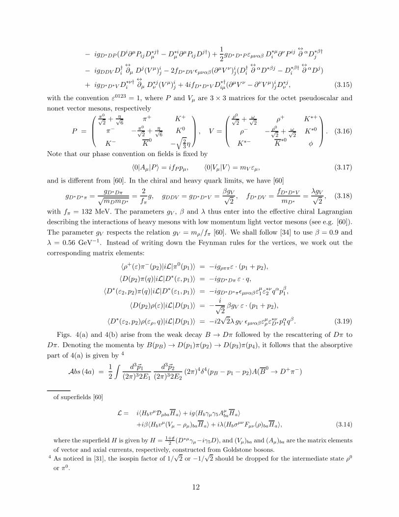
with the convention ε0123 = 1, where P and Vµ are 3 × 3 matrices for the octet pseudoscalar and

nonet vector mesons, respectively

P =

π0√2+ η√

6π+ K+

π− − π0√2+ η√

6K0

K− K0 −

√

23η

, V =

ρ0√2+ ω√

2ρ+ K∗+

ρ− − ρ0√2+ ω√

2K∗0

K∗− K∗0

φ

. (3.16)

Note that our phase convention on fields is fixed by

〈0|Aµ|P 〉 = ifPpµ, 〈0|Vµ|V 〉 = mV εµ, (3.17)

and is different from [60]. In the chiral and heavy quark limits, we have [60]

gD∗D∗π =gD∗Dπ√mDmD∗

=2

fπg, gDDV = gD∗D∗V =

βgV√2, fD∗DV =

fD∗D∗V

mD∗=λgV√

2, (3.18)

with fπ = 132 MeV. The parameters gV , β and λ thus enter into the effective chiral Lagrangian

describing the interactions of heavy mesons with low momentum light vector mesons (see e.g. [60]).

The parameter gV respects the relation gV = mρ/fπ [60]. We shall follow [34] to use β = 0.9 and

λ = 0.56 GeV−1. Instead of writing down the Feynman rules for the vertices, we work out the

corresponding matrix elements:

〈ρ+(ε)π−(p2)|iL|π0(p1)〉 = −igρππε · (p1 + p2),

〈D(p2)π(q)|iL|D∗(ε, p1)〉 = −igD∗Dπ ε · q,〈D∗(ε2, p2)π(q)|iL|D∗(ε1, p1)〉 = −igD∗D∗πǫµναβε

µ1ε

∗ν2 q

αpβ1 ,

〈D(p2)ρ(ε)|iL|D(p1)〉 = − i√2βgV ε · (p1 + p2),

〈D∗(ε2, p2)ρ(ερ, q)|iL|D(p1)〉 = −i2√2λ gV ǫµναβε

µρε

∗νD∗pα1 q

β. (3.19)

Figs. 4(a) and 4(b) arise from the weak decay B → Dπ followed by the rescattering of Dπ to

Dπ. Denoting the momenta by B(pB) → D(p1)π(p2) → D(p3)π(p4), it follows that the absorptive

part of 4(a) is given by 4

Abs (4a) =1

2

∫

d3~p1(2π)32E1

d3~p2(2π)32E2

(2π)4δ4(pB − p1 − p2)A(B0 → D+π−)

of superfields [60]

L = i〈HbvµDµbaHa〉+ ig〈Hbγµγ5A

µbaHa〉

+iβ〈Hbvµ(Vµ − ρµ)baHa〉+ iλ〈Hbσ

µνFµν(ρ)baHa〉, (3.14)

where the superfield H is given byH = 1+v/2 (D∗µγµ−iγ5D), and (Vµ)ba and (Aµ)ba are the matrix elements

of vector and axial currents, respectively, constructed from Goldstone bosons.4 As noticed in [31], the isospin factor of 1/

√2 or −1/

√2 should be dropped for the intermediate state ρ0

or π0.

12

× i1√2βgV

F 2(t,mρ)

t−m2ρ + imρΓρ

(−i)gρππ (p1 + p3)µ(p2 + p4)

ν

(

−gµν +kµkνm2ρ

)

=

∫ 1

−1

|~p1|d cos θ16πmB

1√2gV gρππβ A(B

0 → D+π−)F 2(t,mρ)

t−m2ρ + imρΓρ

H1, (3.20)

where θ is the angle between ~p1 and ~p3, k is the momentum of the exchanged ρ meson (k2 = t),

and

t ≡ (p1 − p3)2 = m2

1 +m23 − 2E1E3 + 2|~p1||~p3| cos θ,

H1 = −(p1 · p2 + p3 · p4 + p1 · p4 + p2 · p3)−(m2

1 −m23)(m

22 −m2

4)

m2ρ

. (3.21)

The form factor F (t,m) in Eq. (3.20) takes care of the off-shell effect of the exchanged particle,

which is usually parametrized as

F (t,m) =

(

Λ2 −m2

Λ2 − t

)n

, (3.22)

normalized to unity at t = m2. The monopole behavior of the form factor (i.e. n = 1) is preferred

as it is consistent with the QCD sum rule expectation [62]. However, we shall return back to this

point when discussing the FSI effects in B → φK∗ decays (see Sec. VII.C).

Likewise, the absorptive part of 4(b) is given by

Abs (4b) =1

2

∫

d3~p1(2π)32E1

d3~p2(2π)32E2

(2π)4δ4(pB − p1 − p2)A(B0 → D+π−)

× igD∗Dπpµ4

F 2(t,mD∗)

t−m2D∗

(−i)gD∗Dπ(−pν2)(

−gµν +kµkνm2D∗

)

= −∫ 1

−1

|~p1|d cos θ16πmB

g2D∗Dπ A(B0 → D+π−)

F 2(t,mD∗)

t−m2D∗

H2, (3.23)

with

H2 = −p2 · p4 +(p2 · p3 −m2

2)(p1 · p4 −m24)

m2D∗

. (3.24)

Figs. 4(c)-4(e) come from the rescattering process B → D∗(p1)ρ(p2) → D(p3)π(p4). The

absorptive part of 4(c) reads

Abs (4c) =1

2

∫

d3~p1(2π)32E1

d3~p2(2π)32E2

(2π)4δ4(pB − p1 − p2)∑

λ1,λ2

A(B0 → D∗+ρ−)

× (−i)gD∗Dπ ε1 · (−p3)F 2(t,mπ)

t−m2π

(−i)gρππ 2ε2 · p4. (3.25)

To proceed, we note that the factorizable amplitude of B → V1V2 is given by

A(B → V1V2) =GF√2VCKM〈V2|(q2q3)V −A

|0〉〈V1|(q1b)V −A|B〉

= −ifV2m2

[

(ε∗1 · ε∗2)(mB +m1)ABV11 (m2

2)− (ε∗1 · pB)(ε∗2 · pB

)2ABV12 (m2

2)

mB +m1

− iǫµναβε∗µ2 ε∗ν1 p

αBpβ1

2V BV1(m22)

mB +m1

]

, (3.26)

13

with (q1q2)V −A≡ q1γµ(1− γ5)q2. Therefore,

Abs (4c) = −i2∫ 1

−1

|~p1|d cos θ16πmB

gD∗DπgρππF 2(t,mπ)

t−m2π

× fρmρ

[

(mB +mD∗)ABD∗

1 (m2ρ)H3 −

2ABD∗

2 (m2ρ)

mB +mD∗H ′

3

]

, (3.27)

where

H3 =

(

p3 · p4 −(p1 · p3)(p1 · p4)

m21

− (p2 · p3)(p2 · p4)m2

2

+(p1 · p2)(p1 · p3)(p2 · p4)

m21m

22

)

,

H ′3 =

(

p2 · p3 −(p1 · p2)(p1 · p3)

m21

)(

p1 · p4 −(p1 · p2)(p2 · p4)

m22

)

. (3.28)

Likewise,

Abs (4d) =1

2

∫

d3~p1(2π)32E1

d3~p2(2π)32E2

(2π)4δ4(pB − p1 − p2)∑

λ1,λ2

A(B0 → D∗+ρ−)

× (−i)gD∗Dπε1 · p4F 2(t,mD∗)

t−m2D∗

(−i) β√2gV ε2 · (k + p3)

= i√2

∫ 1

−1

|~p1|d cos θ16πmB

β gV gD∗DπF 2(t,mD)

t−m2D

× fρmρ

[

(mB +mD∗)ABD∗

1 (m2ρ)H4 −

2ABD∗

2 (m2ρ)

mB +mD∗H ′

4

]

, (3.29)

where H4 and H ′4 can be obtained from H3 and H ′

3, respectively, by interchanging p3 and p4, and

Abs (4e) =1

2

∫

d3~p1(2π)32E1

d3~p2(2π)32E2

(2π)4δ4(pB − p1 − p2)∑

λ1,λ2

A(B0 → D∗+ρ−)

× igD∗D∗π ǫµναβεµ1 p

α4 p

β1

F 2(t,mD∗)

t−m2D∗

i2√2λ gV ǫρσξηε

ρ2pξ3(−p2)η

(

−gνσ + kνkσ

m2D∗

)

= i2√2

∫ 1

−1

|~p1|d cos θ16πmB

gV λ gD∗D∗πF 2(t,mD∗)

t−m2D∗

× fρmρ

[

(mB +mD∗)ABD∗

1 (m2ρ)H5 −

2ABD∗

2 (m2ρ)

mB +mD∗H ′

5

]

, (3.30)

where

H5 = 2(p1 · p2)(p3 · p4)− 2(p1 · p3)(p2 · p4),H ′

5 = m2B

[

(p1 · p2)(p3 · p4)− (p1 · p4)(p2 · p4)]

+ (p2 · pB)(p4 · pB)(p1 · p3) (3.31)

+ (p1 · pB)(p3 · pB)(p2 · p4)− (p1 · pB)(p2 · pB)(p3 · p4)− (p3 · pB)(p4 · pB)(p1 · p2).

Fig. 4(f) comes from the weak decay B0 → D∗+a−1 followed by a strong scattering. We obtain

Abs (4f) =1

2

∫

d3~p1(2π)32E1

d3~p2(2π)32E2

(2π)4δ4(pB − p1 − p2)∑

λ1,λ2

A(B0 → D∗+a−1 ) (3.32)

× i2√2gV λǫµναβε

µ1 p

α3k

β F 2(t,mρ)

t−m2ρ + imρΓρ

(gGρσ + ℓLρσ)ερ2

(

−gνσ + kνkσ

m2D∗

)

14

where

Gρσ = δρσ − 1

Y

[

m22kρkσ + k2pρ2p

σ2 + p2 · k(pρ2kσ + kρpσ2 )

]

Lρσ =p2 · kY

(

pρ2 + kρm2

2

p2 · k

)(

kσ + pσ2k2

p2 · k

)

, (3.33)

and Y = (p2 · k)2 − k2m22. The parameters g and ℓ appearing in Eq. (3.32) also enter into the

strong decay amplitude of a1 → ρπ parametrized as

A(a1 → ρπ) = (gGµν + ℓLµν)εµa1ε

νρ (3.34)

and hence they can determined from the measured decay rate and the ratio of D and S waves:

Γ(a1 → ρπ) =pc

12πm2a1

(

2|g|2 +m2a1m

2ρ

(pa1 · pρ)2|ℓ|2)

,

D

S= −

√2

(Eρ −mρ)g + p2cma1h

(Eρ + 2mρ)g + p2cma1h, (3.35)

with pc being the c.m. momentum of the ρ or π in the a1 rest frame, and

h =pa1 · pρY

(

−g + ℓm2a1m

2ρ

(pa1 · pρ)2

)

. (3.36)

Hence, Eq. (3.32) can be recast to

Abs (4f) = i2√2

∫ 1

−1

|~p1|d cos θ16πmB

gV λ fa1ma1

F 2(t,mρ)

t−m2ρ + imρΓρ

2V BD∗(m2

a1)

mB +mD∗H6, (3.37)

with

H6 =

(

g

Yp2 · k −

ℓ

Y

m22k

2

p2 · k

)

[

m21(p2 · p4)(p2 · p3) +m2

2(p1 · p3)(p1 · p4) + (p1 · p2)2p3 · p4

− m21m

22 p3 · p4 − (p2 · p4)(p1 · p3)(p1 · p2)− (p1 · p2)(p2 · p3)(p1 · p4)

]

− 2g(

m21p2 · p3 − (p1 · p2)(p1 · p3)

)

. (3.38)

It should be emphasized that attention must be paid to the relative sign between B → PP and

B → V V decay amplitudes when calculating long-distance contributions from various rescattering

processes. For the one-body matrix element defined by 〈0|qγµγ5|P 〉 = ifP qµ, the signs of B → PP

and B → V V amplitudes, respectively, are fixed as in Eqs. (3.8) and (3.26). This can be checked

explicitly via heavy quark symmetry (see e.g. [63]).

The dispersive part of the rescattering amplitude can be obtained from the absorptive part via

the dispersion relation

DisA(m2B) =

1

π

∫ ∞

s

AbsA(s′)s′ −m2

B

ds′. (3.39)

Unlike the absorptive part, it is known that the dispersive contribution suffers from the large

uncertainties due to some possible subtractions and the complication from integrations. For this

reason, we will assume the dominance of the rescattering amplitude by the absorptive part and

ignore the dispersive part in the present work except for the decays B0 → π+π− and B0 → π0π0

where a dispersive contribution arising from DD → ππ and ππ → ππ rescattering via annihilation

may play an essential role.

15

B. Numerical results

To estimate the contributions from rescattering amplitudes we need to specify various parameters

entering into the vertices of Feynman diagrams. The on-shell strong coupling gρππ is determined

from the ρ→ ππ rate to be gρππ = 6.05 ± 0.02. The coupling gD∗Dπ has been extracted by CLEO

to be 17.9± 0.3± 1.9 from the measured D∗+ width [64]. The parameters relevant for the D∗D(∗)ρ

couplings are gV = 5.8, β = 0.9 and λ = 0.56GeV−1.

For form factors we use the values determined from the covariant light-front model [63]. For the

coefficients g and ℓ in Eq. (3.34), one can use the experimental results of D/S = −0.1± 0.028 and

Γ(a1 → ρπ) = 250− 600 MeV [50] to fix them. Specifically, we use D/S = −0.1 and Γ(a1 → ρπ) =

400 MeV to obtain g = 4.3 and ℓ = 5.8 . For decay constants, we use fπ = 132 MeV, fD = 200

MeV, fD∗ = 230 MeV and fa1 = −205 MeV.5

Since the strong vertices are determined for physical particles and since the exchanged particle

is not on-shell, it is necessary to introduce the form factor F (t) to account for the off-shell effect

of the t-channel exchanged particle. For the cutoff Λ in the form factor F (t) [see Eq. (3.22)], Λ

should be not far from the physical mass of the exchanged particle. To be specific, we write

Λ = mexc + ηΛQCD, (3.40)

where the parameter η is expected to be of order unity and it depends not only on the exchanged

particle but also on the external particles involved in the strong-interaction vertex. Since we do

not have first-principles calculations of η, we will determine it from the measured branching ratios

given in (3.3) and (3.4). Taking ΛQCD = 220 MeV, we find η = 2.2 for the exchanged particles D∗

and D and η = 1.1 for ρ and π. As noted in passing, the loop corrections will be larger than the

initial B → Dπ amplitudes if the off-shell effect is not considered. Although the strong couplings are

large in the magnitude, the rescattering amplitude is suppressed by a factor of F 2(t) ∼ m2Λ2QCD/t

2.

Consequently, the off-shell effect will render the perturbative calculation meaningful.

Numerically, we obtain (in units of GeV)

A(B0 → D+π−) = i6.41 × 10−7 − (0.90 + i0.09) × 10−7,

A(B0 → D0π0) = −i0.91× 10−7 − 1.56× 10−7,

A(B− → D0π−) = i7.69 × 10−7 + (1.30 − i0.09) × 10−7 (3.41)

for a1 = 0.90 and a2 = 0.25,6 where the first term on the right hand side of each amplitude

arises from the short-distance factorizable contribution and the second term comes from absorptive

parts of the final-state rescattering processes. Note that the absorptive part of B0 → D+π− and

B− → D0π− decay amplitudes are complex owing to a non-vanishing ρ width. To calculate the

5 The sign of fa1is opposite to fπ as noticed in [63].

6 As mentioned before, a2(Dπ) is a priori not calculable in the QCD factorization approach. Therefore,

we choose a2(Dπ) ≈ 0.25 for the purpose of illustration. Nevertheless, a rough estimate of a2(Dπ) has

been made in [17] by treating the charmed meson as a light meson while keeping its highly asymmetric

distribution amplitude. It yields a2(Dπ) ≈ 0.25 exp(−i40◦).

16

branching ratios, we will take into account the uncertainty from the ΛQCD scale. Recall that

ΛQCD = 217+25−21 MeV is quoted in PDG [50]. Therefore, allowing 15% error in ΛQCD, the flavor-

averaged branching ratios are found to be

B(B0 → D+π−) = (3.1+0.0−0.0)× 10−3 (3.2 × 10−3),

B(B− → D0π−) = (5.0+0.1−0.0)× 10−3 (4.9 × 10−3),

B(B0 → D0π0) = (2.5+1.1−0.8)× 10−4 (0.6 × 10−4), (3.42)

where the branching ratios for decays without FSIs are shown in parentheses. We see that the D0π0

mode is sensitive to the cutoff scales ΛD∗ and ΛD, whereas the other two color-allowed channels are

not. It is clear that the naively predicted B(B0 → D0π0) before taking into account rescattering

effects is too small compared to experiment. In contrast, B0 → D+π− and B− → D0π− are almost

not affected by final-state rescattering. Moreover,

CT

∣

∣

∣

∣

Dπ=

{

0.28 e−i48◦,

0.20,

ET

∣

∣

∣

∣

Dπ=

{

0.14 ei96◦, with FSI

0, without FSI(3.43)

where we have assumed negligible short-distance W -exchange and taken the central values of the

cutoffs. Evidently, even if the short-distance weak annihilation vanishes, a long-distance contribu-

tion to W -exchange can be induced from rescattering. Consequently,

C − ET + E

∣

∣

∣

∣

Dπ=

{

0.40 e−i67◦,

0.20,

C − ET + C

∣

∣

∣

∣

Dπ=

{

0.33 e−i50◦, with FSI

0.17, without FSI(3.44)

Therefore, our results are consistent with experiment (3.5). This indicates that rescattering will

enhance the ratios and provide the desired strong phases. That is, the enhancement of R ≡(C−E)/(T +E) relative to the naive expectation is ascribed to the enhancement of color-suppressed

W -emission and the long-distance W -exchange, while the phase of R is accounted for by the strong

phases of C and E topologies.

Because the rescattering long-distance amplitudes have the same weak phases as the short-

distance factorizable ones, it is clear that there is no direct CP violation induced from rescattering

FSIs.

Since the decay B0 → D+

s K− proceeds only through the topological W -exchange diagram, the

above determination of E allows us to estimate its decay rate. From Eq. (3.43) it follows that

|E/(T + E)|2 = 0.020 in the presence of FSIs. Therefore, we obtain

Γ(B0 → D+

s K−)

Γ(B0 → D+π−)

= 0.019 , (3.45)

which is indeed consistent with the experimental value of 0.014 ± 0.005 [50]. The agreement will

be further improved after taking into account SU(3) breaking in the E amplitude of B0 → D+

s K−.

IV. B → πK DECAYS

The penguin dominated B → πK decay amplitudes have the general expressions

17

TABLE I: Experimental data for CP averaged branching ratios (top, in units of 10−6) and CP asym-

metries (bottom) for B → πK [50, 65].

Mode BaBar Belle CLEO Average

B− → π−K0

26.0 ± 1.3± 1.0 22.0 ± 1.9 ± 1.1 18.8+3.7+2.1−3.3−1.8 24.1 ± 1.3

B0 → π+K− 17.9 ± 0.9± 0.7 18.5 ± 1.0 ± 0.7 18.0+2.3+1.2

−2.1−0.9 18.2 ± 0.8

B− → π0K− 12.0 ± 0.7± 0.6 12.0 ± 1.3+1.3−0.9 12.9+2.4+1.2

−2.2−1.1 12.1 ± 0.8

B0 → π0K

011.4 ± 0.9± 0.6 11.7 ± 2.3+1.2

−1.3 12.8+4.0+1.7−3.3−1.4 11.5 ± 1.0

Aπ−KS−0.087 ± 0.046 ± 0.010 0.05 ± 0.05 ± 0.01 0.18± 0.24 ± 0.02 −0.020 ± 0.034

Aπ+K− −0.133 ± 0.030 ± 0.009 −0.101 ± 0.025 ± 0.005 −0.04 ± 0.16 ± 0.02 −0.113 ± 0.019

Aπ0K− 0.06 ± 0.06 ± 0.01 0.04 ± 0.05 ± 0.02 −0.29 ± 0.23 ± 0.02 0.04 ± 0.04

Aπ0KS−0.06 ± 0.18 ± 0.06 −0.12± 0.20 ± 0.07 −0.09± 0.14

Sπ0KS0.35+0.30

−0.33 ± 0.04 0.30 ± 0.59 ± 0.11 0.34+0.27−0.29

A(B0 → π+K−) = T + P +

2

3P ′EW + PA,

A(B0 → π0K

0) =

1√2(C − P + PEW +

1

3P ′EW − PA), (4.1)

A(B− → π−K0) = P − 1

3P ′EW +A+ PA,

A(B− → π0K−) =1√2(T + C + P + PEW +

2

3P ′EW +A+ PA),

where PEW and P ′EW are color-allowed and color-suppressed electroweak penguin amplitudes, re-

spectively, and PA is the penguin-induced weak annihilation amplitude. The decay amplitudes

satisfy the isospin relation

A(B0 → π+K−) +

√2A(B

0 → π0K0) = −A(B− → π−K

0) +

√2A(B− → π0K−). (4.2)

Likewise, a similar isospin relation holds for charge conjugate fields

A(B0 → π−K+) +√2A(B0 → π0K

0) = −A(B+ → π+K0) +

√2A(B+ → π0K+). (4.3)

In the factorization approach [66, 67],

TSD = κ1λua1, CSD = κ2λua2, PSD = κ1[

λu(au4 + au6r

Kχ ) + λc(a

c4 + ac6r

Kχ )]

,

PSDEW =

3

2κ2(λu + λc)(−a7 + a9), P ′SD

EW =3

2κ1[

λu(au8rKχ + au10) + λc(a

c8rKχ + ac10)

]

, (4.4)

with λq ≡ V ∗qsVqb, r

Kχ = 2m2

K/[mb(µ)(ms +mq)(µ)], and

κ1 = iGF√2fKF

Bπ0 (m2

K)(m2B −m2

π), κ2 = iGF√2fπF

BK0 (m2

π)(m2B −m2

K). (4.5)

The parameters au,ci can be calculated in the QCD factorization approach [17]. They are basically

the Wilson coefficients in conjunction with short-distance nonfactorizable corrections such as vertex

18

��✒

��

❅❅❘

❅❅

❄

✲

✲

B

η′

K

K∗

K

π

(a)

��✒

��

❅❅❘

❅❅

❄

✲

✲

B

Ds

D

D∗

K

π

(b)

��✒

��

❅❅❘

❅❅

❄

✲

✲

B

D∗

s

D∗

D

K

π

(c)

��✒

��

❅❅❘

❅❅

❄

✲

✲

B

D∗

s

D∗

D∗

K

π

(d)

FIG. 5: Long-distance t-channel rescattering contributions to B → Kπ.

corrections and hard spectator interactions. Formally, ai(i 6= 6, 8) and a6,8rKχ should be renormal-

ization scale and scheme independent. In practice, there exists some residual scale dependence in

ai(µ) to finite order. At the scale µ = 2.1 GeV, the numerical results are

a1 = 0.9921 + i0.0369, a2 = 0.1933 − i0.1130, a3 = −0.0017 + i0.0037,

au4 = −0.0298 − i0.0205, ac4 = −0.0375 − i0.0079, a5 = 0.0054 − i0.0050,

au6 = −0.0586 − i0.0188, ac6 = −0.0630 − i0.0056, a7 = i5.4 × 10−5,

au8 = (45.0 − i5.2) × 10−5, ac8 = (44.2 + i3.1) × 10−5, a9 = −(953.9 + i24.5) × 10−5,

au10 = (−58.3 + i86.1) × 10−5, ac10 = (−60.3 + i88.8) × 10−5. (4.6)

For current quark masses, we use mb(mb) = 4.4 GeV, mc(mb) = 1.3 GeV, ms(2.1GeV) = 90 MeV

and mq/ms = 0.044.

Using the above coefficients au,ci leads to

B(B− → π−K0)SD = 17.8 × 10−6, ASD

π−KS= 0.01,

B(B0 → π+K−)SD = 13.9 × 10−6, ASDπ+K− = 0.04,

B(B− → π0K−)SD = 9.7 × 10−6, ASDπ0K− = 0.08,

B(B0 → π0K0)SD = 6.3 × 10−6, ASD

π0KS= −0.04 , (4.7)

where we have used |Vcb| = 0.041, |Vub/Vcb| = 0.09 and γ = 60◦ for quark mixing matrix elements.7

From Table I it is clear that the predicted branching ratios are slightly smaller than experiment

especially for B0 → π0K

0where the prediction is about two times smaller than the data. Moreover,

the predicted CP asymmetry for π+K− is opposite to the experimental measurement in sign. By

now, direct CP violation in B0 → π+K− has been established by both BaBar [14] and Belle [15].

7 The notations (α, β, γ) and (φ1, φ2, φ3) with α ≡ φ2, β ≡ φ1, γ ≡ φ3 are in common usage for the angles

of the unitarity triangle.

19

Leading long-distance rescattering contributions toB → Kπ are shown in Fig. 5. The absorptive

amplitudes are

Abs (5a) = −∫ 1

−1

|~p1|d cos θ16πmB

gK∗Kπ gK∗Kη′A(B0 → K

0η′)

F 2(t,mρ)

t−m2K∗

H1,

Abs (5b) =

∫ 1

−1

|~p1|d cos θ16πmB

gD∗Dπ gD∗DsKA(B0 → D+D−

s )F 2(t,mD∗)

t−m2D∗

J2, (4.8)

Abs (5c) = −iGF√2VcbV

∗csfD∗

smD∗

s

∫ 1

−1

|~p1|d cos θ16πmB

gD∗Dπ gD∗sDK

F 2(t,mD)

t−m2D

×[

(mB +mD∗)ABD∗

1 (m2D∗

s)H4 −

2ABD∗

2 (m2D∗

s)

mB +mD∗H ′

4

]

,

Abs (5d) = iGF√2VcbV

∗csfD∗

smD∗

s

∫ 1

−1

|~p1|d cos θ16πmB

gD∗D∗π gD∗sDK

F 2(t,mD∗)

t−m2D∗

×[

(mB +mD∗)ABD∗

1 (m2D∗

s)J5 −

2ABD∗

2 (m2D∗

s)

mB +mD∗J ′5

]

,

with

J2 = −p3 · p4 −(p1 · p3 −m2

3)(p2 · p4 −m24)

m2D∗

, (4.9)

and J5, J′5 can be obtained from H5 and H ′

5, respectively, under the replacement of p3 ↔ p4.

Hence,

A(B− → π−K0) = A(B− → π−K

0)SD + iAbs(5a+ 5b+ 5c+ 5d),

A(B0 → π+K−) = A(B

0 → π+K−)SD + iAbs(5a+ 5b+ 5c+ 5d),

A(B− → π0K−) = A(B− → π0K−)SD +i√2Abs(5a+ 5b+ 5c+ 5d),

A(B0 → π0K

0) = A(B

0 → π0K0)SD − i√

2Abs(5a+ 5b+ 5c+ 5d). (4.10)

As noticed before, the rescattering diagrams 5(b)-5(d) with charm intermediate states contribute

only to the topological penguin graph. Indeed, it has been long advocated that charming-penguin

long-distance contributions increase significantly the B → Kπ rates and yield better agreement

with experiment [33]. For a recent work along this line, see [34].

To proceed with the numerical calculation, we use the experimental value A(B0 → K

0η′) =

(−7.8+ i4.5)×10−8 GeV with the phase determined from the topological approach [10]. For strong

couplings, gK∗Kπ defined for K∗+ → K0π+ is fixed to be 4.6 from the measured K∗ width, and

the K∗Kη′ coupling is fixed to be

gK∗+→K+η′ =1√3gK∗+→K+π0 =

1√6gK∗+→K0π+ (4.11)

by approximating the η′ wave function by η′ = 1√6(uu+ dd+2ss). A χ2 fit to the measured decay

rates yields ηD(∗) = 0.69 for the exchanged particle D or D∗, while ηK∗ is less constrained as the

exchanged K∗ particle contribution [Fig. 5(a)] is suppressed relative to the D or D∗ contribution.

Since the decay B → DDs is quark-mixing favored over B → Dπ, the cutoff scale here thus should

be lower than that in B → Dπ decays where ηD(∗) = 2.2 as it should be. As before, we allow 15%

20

TABLE II: Comparison of experimental data and fitted outputs for CP averaged branching ratios

(top, in units of 10−6) and the theoretical predictions of CP asymmetries (bottom) for B → πK.

Mode Expt. SD SD+LD

B(B− → π−K0) 24.1 ± 1.3 17.8 23.3+4.6

−3.7

B(B0 → π+K−) 18.2 ± 0.8 13.9 19.3+5.0−3.1

B(B− → π0K−) 12.1 ± 0.8 9.7 12.5+2.6−1.6

B(B0 → π0K0) 11.5 ± 1.0 6.3 9.1+2.5

−1.6

Aπ−KS−0.02± 0.03 0.01 0.024+0.0

−0.001

Aπ+K− −0.11± 0.02 0.04 −0.14+0.01−0.03

Aπ0K− 0.04 ± 0.04 0.08 −0.11+0.02−0.04

Aπ0KS−0.09± 0.14 −0.04 0.031+0.008

−0.014

Sπ0KS0.34 ± 0.28 0.79 0.78 ± 0.01

uncertainty for the ΛQCD scale and obtain the branching ratios and CP asymmetries as shown

in Table II, where use has been made of fD∗s≈ fDs

= 230 MeV and the heavy quark symmetry

relations

gD∗DsK =

√

mDs

mDgD∗Dπ, gD∗

sDK =

√

mD∗s

mD∗gD∗Dπ. (4.12)

It is found that the absorptive contribution from the Kη′ intermediate states is suppressed relative

to D(∗)D(∗)s as the latter are quark-mixing-angle most favored, i.e. B → D(∗)D

(∗)s ≫ B → Kη′.

Evidently, all πK modes are sensitive to the cutoffs ΛD∗ and ΛD. We see that the sign of the direct

CP partial rate asymmetry for B0 → π+K− is flipped after the inclusion of rescattering and the

predicted Aπ+K− = −0.14+0.01−0.03 is now in good agreement with the world average of −0.11 ± 0.02.

Note that the branching ratios for all πK modes are enhanced by (30 ∼ 40)% via final-state

rescattering.

Note that there is a sum-rule relation [28]

2∆Γ(π0K−)−∆Γ(π−K0)−∆Γ(π+K−) + 2∆Γ(π0K

0) = 0, (4.13)

based on isospin symmetry. Hence, a violation of the above relation would provide an important

test for the presence of electroweak penguin contributions. It is interesting to check how good the

above relation works in light of the present data. We rewrite it as

Aπ+K−B(π+K−)− 2Aπ0K

0B(π0K0)

2Aπ0K−B(π0K−)−Aπ−K

0B(π−K0)=τB

0

τB−

. (4.14)

The left hand side of the above equation yields 0.07 ± 2.28, while the right hand side is 0.923 ±0.014 [50]. Although the central values of the data seem to imply the need of non-vanishing

electroweak penguin contributions and/or some New Physics, it is not conclusive yet with present

data. For further implications of this sum-rule relation, see [28].

21

TABLE III: Experimental data for CP averaged branching ratios (top, in units of 10−6) and

CP asymmetries (bottom) for B → ππ [50, 65].

Mode BaBar Belle CLEO Average

B0 → π+π− 4.7± 0.6 ± 0.2 4.4± 0.6± 0.3 4.5+1.4+0.5

−1.2−0.4 4.6± 0.4

B0 → π0π0 1.17 ± 0.32 ± 0.10 2.32+0.44+0.22

−0.48−0.18 < 4.4 1.51 ± 0.28

B− → π−π0 5.8± 0.6 ± 0.4 5.0± 1.2± 0.5 4.6+1.8+0.6−1.6−0.7 5.5± 0.6

Aπ+π− 0.09 ± 0.15 ± 0.04 0.58± 0.15 ± 0.07 0.31 ± 0.24a

Sπ+π− −0.30 ± 0.17 ± 0.03 −1.00 ± 0.21 ± 0.07 −0.56± 0.34a

Aπ0π0 0.12 ± 0.56 ± 0.06 0.43 ± 0.51+0.17−0.16 0.28 ± 0.39

Aπ−π0 −0.01 ± 0.10 ± 0.02 −0.02 ± 0.10 ± 0.01 −0.02 ± 0.07

aError-bars of Aπ+π− and Sπ+π− are scaled by S = 2.2 and 2.5, respectively. When taking into account

the measured correlation between A and S, the averages are cited by Heavy Flavor Averaging Group [65] to

be Aπ+π− = 0.37± 0.11 and Sπ+π− = −0.61± 0.14 with errors not being scaled up.

V. B → ππ DECAYS

A. Short-distance contributions and Experimental Status

The experimental results of CP averaged branching ratios and CP asymmetries for charmless

B → ππ decays are summarized in Table III. For a neutral B meson decay into a CP eigenstate

f , CP asymmetry is defined by

Γ(B(t) → f)− Γ(B(t) → f)

Γ(B(t) → f) + Γ(B(t) → f)= Sf sin(∆mt)− Cf cos(∆mt), (5.1)

where ∆m is the mass difference of the two neutral B eigenstates, Sf is referred to as mixing-induced

CP asymmetry and Af = −Cf is the direct CP asymmetry. Note that the Belle measurement [12]

gives an evidence of CP violation in B0 → π+π− decays at the level of 5.2 standard deviations,

while this has not been confirmed by BaBar [20]. As a result, we follow Particle Data Group [50]

to use a scale factor of 2.2 and 2.5, respectively, for the error-bars in Aπ+π− and Sπ+π− (see Table

III). The CP -violating parameters Cf and Sf can be expressed as

Cf =1− |λf |21 + |λf |2

, Sf =2 Imλf1 + |λf |2

, (5.2)

where

λf =q

p

A(B0 → f)

A(B0 → f). (5.3)

For ππ modes, q/p = e−i2β with sin 2β = 0.726 ± 0.037 [68].

The B → ππ decay amplitudes have the general expressions

A(B0 → π+π−) = T + P +

2

3P ′EW + E + PA + V,

22

A(B0 → π0π0) = − 1√

2(C − P + PEW +

1

3P ′EW − E − PA − V), (5.4)

A(B− → π−π0) =1√2(T + C + PEW + P ′

EW),

where V is the vertical W -loop topological diagram (see Sec. II). In the factorization approach, the

quark diagram amplitudes are given by [66, 67]

TSD = κλua1, CSD = κλua2, PSD = κ[

λu(au4 + au6r

πχ) + λc(a

c4 + ac6r

πχ)]

,

PSDEW =

3

2κ(λu + λc)(−a7 + a9), P ′SD

EW =3

2κ[

λu(au8rπχ + au10) + λc(a

c8rπχ + ac10)

]

, (5.5)

where λq ≡ V ∗qdVqb, κ ≡ iGF√

2fπF

Bπ0 (m2

π)(m2B − m2

π) and the chiral enhancement factor rπχ =

2m2π/[mb(µ)(mu +md)(µ)] arises from the (S − P )(S + P ) part of the penguin operator Q6. The

explicit expressions of the weak annihilation amplitude E in QCD factorization can be found in

[17]. It is easily seen that the decay amplitudes satisfy the isospin relation

A(B0 → π+π−) =

√2[

A(B− → π−π0) +A(B0 → π0π0)

]

. (5.6)

Note that there is another isospin relation for charge conjugate fields

A(B0 → π+π−) =√2[

A(B+ → π+π0) +A(B0 → π0π0)]

. (5.7)

Substituting the coefficients au,ci given in Eq. (4.6) into Eqs. (5.4) and (5.5) leads to8

B(B0 → π+π−)SD = 7.6× 10−6, ASDπ+π− = −0.05,

B(B0 → π0π0)SD = 2.7× 10−7, ASDπ0π0 = 0.61, (5.8)

B(B− → π−π0)SD = 5.1× 10−6, ASDπ−π0 = 5× 10−5.

To obtain the above branching ratios and CP asymmetries we have applied the form factor

FBπ0 (0) = 0.25 as obtained from the covariant light-front approach [63] and neglected the W -

annihilation contribution. Nevertheless, the numerical results are similar to that in [18] (see Tables

9 and 10 of [18]) except for Aπ−π0 for which we obtain a sign opposite to [18].

We see that the predicted π+π− rate is too large, whereas π0π0 is too small compared to

experiment (see Table III). Furthermore, the predicted value of direct CP asymmetry, ASDπ+π− =

−0.05, is in disagreement with the experimental average of 0.31 ± 0.24. 9 In the next subsection,

we will study the long-distance rescattering effect to see its impact on CP violation.

In the topological analysis in [10], it is found that in order to describe B → ππ and B → πK

branching ratios and CP asymmetries, one must introduce a large value of |C/T | and a non-trivial

phase between C and T . Two different fit procedures have been adopted in [10] to fit ππ and πK

8 Charge conjugate modes are implicitly included in the flavor-averaged branching ratios throughout this

paper.9 In the so-called perturbative QCD approach for nonleptonic B decays [69], the signs of π+π− and K−π+

CP asymmetries are correctly predicted and the calculated magnitudes are compatible with experiment.

23

��✒

��

❅❅❘

❅❅

❄

✲

✲

B

π

π

ρ

π

π

(a)

��✒

��

❅❅❘

❅❅

❄

✲

✲

B

ρ

ρ

π

π

π

(b)

��✒

��

❅❅❘

❅❅

❄

✲

✲

B

D

D

D∗

π

π

(c)

��✒

��

❅❅❘

❅❅

❄

✲

✲

B

D∗

D∗

D(D∗)

π

π

(d),(e)

FIG. 6: Long-distance t-channel rescattering contributions to B → ππ. Graphs (d) and (e) corre-

spond to the exchanged particles D and D∗, respectively.

dd

B0

π+

π−

π0

d

π0

d

ub

udu

ud

B0

π+

π−

π0

u

π0

u

ub

dud

(a) (b)

FIG. 7: Contributions to B0 → π0π0 from the color-allowed weak decay B

0 → π+π− followed

by quark annihilation processes (a) and (b). They have the same topologies as the penguin and

W -exchange graphs, respectively.

data points by assuming negligible weak annihilation contributions. One of the fits yields10

γ = (65+13−35)

◦,CT

∣

∣

∣

∣

ππ,πK= (0.46+0.43

−0.30) exp[−i(94+43−52)]

◦. (5.9)

The result for the ratio C/T in charmless B decays is thus consistent with (3.5) extracted from

B → Dπ.

B. Long-distance contributions to B → ππ

Some leading rescattering contributions to B → ππ are shown in Figs. 6(a)-6(e). While all

the five diagrams contribute to B0 → π+π− and B

0 → π0π0, only the diagrams 6(a) and 6(b)

contribute to B− → π−π0. Since the π−π0 final state in B− decay must be in I = 2, while the

10 The other fit yields |C/T | = 1.43+0.40−0.31 which is unreasonably too large. This ratio is substantially reduced

once the up and top quark mediated penguins are taken into account [10].

24

intermediate DD state has I = 0 or I = 1, it is clear that B− → π−π0 cannot receive rescattering

from B− → D−D0 → π−π0. It should be stressed that all the graphs in Fig. 6 contribute to the

penguin amplitude. To see this, let us consider Fig. 7 which is one of the manifestations of Fig.

6(a) at the quark level. (Rescattering diagrams with quark exchange are not shown in Fig. 7.)

It is easily seen that Figs. 7(a) and 7(b) can be redrawn as the topologies P and E , respectively.Likewise, Figs. 6(c)-(e) correspond to the topological P. Consequently,

T = TSD,C = CSD + iAbs (6a+ 6b), (5.10)

E = ESD + iAbs (6a+ 6b),

P = PSD + iAbs (6a+ 6b+ 6c+ 6d+ 6e).

Hence,11

A(B0 → π+π−) = A(B

0 → π+π−)SD + 2iAbs (6a+ 6b) + iAbs(6c+ 6d+ 6e),

A(B0 → π0π0) = A(B

0 → π0π0)SD +1√2iAbs (6a+ 6b+ 6c+ 6d+ 6e), (5.11)

A(B− → π−π0) = A(B− → π−π0)SD +1√2iAbs (6a+ 6b),

The absorptive parts of B → M1(p1)M2(p2) → π(p3)π(p4) with M1,2 being the intermediate

states in Fig. 6 are

Abs (6a) = −∫ 1

−1

|~p1|d cos θ16πmB

g2ρππA(B0 → π+π−)

F 2(t,mρ)

t−m2ρ + imρΓρ

H1,

Abs (6b) = −iGF√2VubV

∗udfρmρ

∫ 1

−1

|~p1|d cos θ16πmB

g2ρππF 2(t,mπ)

t−m2π

×[

(mB +mρ)ABρ1 (m2

π)4H3 −2ABρ2 (m2

π)

mB +mρ4H ′

3

]

,

Abs (6c) =

∫ 1

−1

|~p1|d cos θ16πmB

g2D∗DπA(B0 → D+D−)

F 2(t,mD∗)

t−m2D∗

J2, (5.12)

Abs (6d) = −iGF√2VcbV

∗cdfD∗mD∗

∫ 1

−1

|~p1|d cos θ16πmB

g2D∗Dπ

F 2(t,mD)

t−m2D

×[

(mB +mD∗)ABD∗

1 (m2D∗)H4 −

2ABD∗

2 (m2D∗)

mB +mD∗H ′

4

]

,

Abs (6e) = iGF√2VcbV

∗cdfD∗mD∗

∫ 1

−1

|~p1|d cos θ16πmB

g2D∗D∗π

F 2(t,mD∗)

t−m2D∗

×[

(mB +mD∗)ABD∗

1 (m2D∗)J5 −

2ABD∗

2 (m2D∗)

mB +mD∗J ′5

]

.

11 In a similar context, it has been argued in [31] that the analogous Figs. 6(a)-(b) do not contribute to the

decay D0 → π0π0 owing to the cancellation between the quark annihilation and quark exchange diagrams

at the quark level. However, a careful examination indicates that the quark annihilation processes gain

an additional factor of 2 as noticed in [38]. Consequently, the intermediate π+π− state does contribute to

B0 → π0π0 and D0 → π0π0 via final-state rescattering.

25

Since in SU(3) flavor limit the final-state rescattering parts of Figs. 6(c)-(e) should be the same

as that of Figs. 5(b)-(d), it means that the cutoff scales ΛD and ΛD∗ appearing in the rescattering

diagrams of B → ππ are identical to that in B → πK decays in the limit of SU(3) symmetry.

Allowing 20% SU(3) breaking and recalling that ηD(∗) = 0.69 in B → πK decays, we choose

ηD(∗) = ηρ = 0.83 for B → ππ decays. Because the decay B0 → D+D− is Cabibbo suppressed

relative to B0 → D+D−

s , it is evident that the absorptive part of the charm loop diagrams, namely,

Figs. 6(c)-(e), cannot enhance the π0π0 rate sizably. However, since the branching ratio of the

short-distance induced B0 → π+π−, namely 7.6×10−6 [see Eq. (5.8)], already exceeds the measured

value substantially, this means that a dispersive part of the long-distance rescattering amplitude

must be taken into account. This dispersive part also provides the main contribution to the π0π0

rate. There is a subtle point here: If the dispersive contribution is fixed by fitting to the measured

B → ππ rates, the χ2 value of order 0.2 is excellent and the predicted direct CP violation for π+π−

agrees with experiment. Unfortunately, the calculated mixing-induced CP -violating parameter S

will have a wrong sign. Therefore, we need to accommodate the data of branching ratios and the

parameter S simultaneously. We find (in units of GeV)

DisA = 1.5× 10−6VcbV∗cd − 6.7 × 10−7VubV

∗ud, (5.13)

for ηπ = ηρ = 1.2. It should be stressed that these dispersive contributions cannot arise from the

rescattering processes in Figs. 6(a)-(e) because they will also contribute to B → Kπ decays via

SU(3) symmetry and modify all the previous predictions very significantly. As pointed out in [38],

there exist ππ → ππ and DD → ππ meson annihilation diagrams in which the two initial quark

pairs in the zero isospin configuration are destroyed and then created. Such annihilation diagrams

have the same topology as the vertical W -loop diagram V as mentioned in Sec. II. Hence, this FSI

mechanism occurs in π+π− and π0π0 but not in the Kπ modes. That is, the dispersive term given

in Eq. (5.13) does not contribute to B → Kπ decays.

The resultant amplitudes are then given by (in units of GeV)12

A(B0 → π+π−) = (2.03 + i2.02) × 10−8 + (1.40 − i0.77) × 10−8 − i1.64 × 10−8,

A(B0 → π+π−) = (−2.21 + i2.04) × 10−8 − (2.21 − i2.05) × 10−8 − i1.64 × 10−8,

A(B0 → π0π0) = (−6.15 + i3.46) × 10−9 + (7.89 − i2.73) × 10−9 − i1.07 × 10−8,

A(B0 → π0π0) = (3.32 + i1.11) × 10−9 + (3.32 + i1.11) × 10−9 − i1.07 × 10−8,

A(B− → π−π0) = (2.05 + i1.08) × 10−8 + (2.07 − i2.73) × 10−9,

A(B+ → π+π0) = (−1.90 + i1.34) × 10−8 − (1.90 − i1.34) × 10−8, (5.14)

where the numbers in the first parentheses on the right hand side are due to short-distance con-

tributions, while the second term in parentheses and the third term arise from the absorptive

and dispersive parts, respectively, of long-distance rescattering. (The dispersive contribution to

B− → π−π0 is too small and can be neglected.) Form the above equation, it is clear that the

12 Note that B → PP and B → V V decay amplitudes are accompanied by a factor of i in our phase

convention [see Eq. (3.8)].

26

TABLE IV: Same as Table II except for B → ππ decays.

Mode Expt. SD SD+LD

B(B0 → π+π−) 4.6± 0.4 7.6 4.6+0.2−0.1

B(B0 → π0π0) 1.5± 0.3 0.3 1.5+0.1−0.0

B(B− → π−π0) 5.5± 0.6 5.1 5.4± 0.0

Aπ+π− 0.31± 0.24 −0.05 0.35+0.15−0.14

Sπ+π− −0.56± 0.34 −0.66 −0.16+0.15−0.16

Aπ0π0 0.28± 0.39 0.56 −0.30+0.01−0.04

Aπ−π0 −0.02± 0.07 5× 10−5 −0.009+0.002−0.001

long-distance dispersive amplitude gives the dominant contribution to π0π0 and contributes de-

structively with the short-distance π+π− amplitude. The corresponding CP averaged branching

ratios and direct CP asymmetries are shown in Table IV, where the ranges indicate the uncertain-

ties of the QCD scale ΛQCD by 15%. We only show the ranges due to the cut-off as numerical

predictions depend sensitively on it. It is evident that the π−π0 rate is not significantly affected by

FSIs, whereas the π+π− and π0π0 modes receive sizable long-distance corrections.13

Since the branching ratio of B0 → D+D− is about 50 times larger than that of B0 → π+π−,

it has been proposed in [35] that a small mixing of the ππ and DD channels can account for the

puzzling observation of B0 → π0π0. However, the aforementioned dispersive part of final-state

rescattering was not considered in [35] and consequently the predicted branching ratio B(B0 →π+π−) ∼ 11 × 10−6 is too large compared to experiment. In the present work, we have shown

that it is the dispersive part of long-distance rescattering from DD → ππ that accounts for the

suppression of the π+π− mode and the enhancement of π0π0.

As far as CP rate asymmetries are concerned, the long-distance effect will generate a sizable

direct CP violation for π+π− with a correct sign. Indeed, the signs of direct CP asymmetries in

B → ππ decays are all flipped by the final-state rescattering effects. It appears that FSIs lead

to CP asymmetries for π+π− and π0π0 opposite in sign. The same conclusion is also reached

in the ππ and DD mixing model [35] and in an analysis of charmless B decay data [38] based

on a quasi-elastic scattering model [57] (see also [40]). However, the perturbative QCD approach

based on the kT factorization theorem predicts the same sign for π+π− and π0π0 CP asymmetries,

namely, Aπ+π− = 0.23±0.07 and Aπ0π0 = 0.30±0.10 [69]. Moreover, a global analysis of charmless

B → PP decays based on the topological approach yields Aπ+π− ∼ 0.33 and Aπ0π0 ∼ 0.53 [10] (see

13 A different mechanism for understanding the ππ data is advocated in [38] where FSI is studied based on

a simple two parameter model by considering a quasi-elastic scattering picture. A simultaneous fit to the

measured rates and CP asymmetries indicates that π+π− is suppressed by the dispersive part of ππ → ππ

rescattering, while π0π0 is enhanced via the absorptive part. This requires a large SU(3) rescattering

phase difference of order 90◦ ∼ 100◦. The fitted π−π0 rate is somewhat below experiment. In the present

work, it is the dispersive part of the rescattering from DD to ππ via annihilation that plays the role for

the enhancement of π0π0 and suppression of π+π−.

27

also [70] for the same conclusion reached in a different context). It is worth mentioning that the

isospin analyses of B → ππ decay data in [71] and [72] all indicate that given the allowed region

of the π0π0 branching ratio, there is practically no constraints on π0π0 direct CP violation from

BaBar and/or Belle data. And hence the sign of Aπ0π0 is not yet fixed. At any rate, even a sign

measurement of direct CP asymmetry in π0π0 will provide a nice testing ground for discriminating

between the FSI and PQCD approaches for CP violation.

It is interesting to notice that based on SU(3) symmetry, there are some model-independent

relations for direct CP asymmetries between ππ and πK modes [73]

∆Γ(π+π−) = −∆Γ(π+K−), ∆Γ(π0π0) = −∆Γ(π0K0), (5.15)

with ∆Γ(f1f2) ≡ Γ(B → f1f2)− Γ(B → f1f2). From the measured rates, it follows that

Aπ+π− ≈ −4.0Aπ+K−, Aπ0π0 ≈ −7.7Aπ0K

0 . (5.16)

It appears that the first relation is fairly satisfied by the world averages of CP asymmetries. Since

direct CP violation in the π+K− mode is now established by B factories, the above relation implies

that the π+π− channel should have Aπ+π− ∼ O(0.4) with a positive sign. For the neutral modes

more data are clearly needed as the current experimental results have very large errors.

Finally we present the results for the ratios C/T , E/T and V/T :

CT

∣

∣

∣

∣

ππ= 0.36 e−i55

◦

,ET

∣

∣

∣

∣

ππ= 0.19 e−i85

◦

,VT

∣

∣

∣

∣

ππ= 0.56 ei230

◦

, (5.17)

to be compared with the short-distance result C/T |SDππ = a2/a1 = 0.23 exp(−i32◦) from Eq. (4.6).

Evidently, the ratio of C/T in B → ππ decays is similar to that in B → Dπ decays [see Eq. (3.43)].

To analyze the B → ππ data, it is convenient to define Teff = T + E + V and Ceff = C − E − V. It

follows from Eq. (5.17) that

CeffTeff

∣

∣

∣

∣

ππ= 0.71 ei72

◦

. (5.18)

This is consistent with Eq. (5.9) obtained from the global analysis of B → ππ and πK data.

C. CP violation in B− → π−π0 decays

We see from Table IV that for B− → π−π0, even including FSIs CP -violating partial-rate

asymmetry in the SM is likely to be very small; the SD contribution ∼ 5 × 10−4 may increase to

the level of one percent. Although this SM CP asymmetry is so small that it is difficult to measure

experimentally, it provides a nice place for detecting New Physics. This is because the isospin of

the π−π0 ( also ρ−ρ0) state in the B decay is I = 2 and hence it does not receive QCD penguin

contributions and receives only the loop contributions from electroweak penguins. Since these

decays are tree dominated, SM predicts an almost null CP asymmetry. Final-state rescattering

can enhance the CP -violating effect at most to one percent level. Hence, a measurement of direct

CP violation in B− → π−π0 provides a nice test of the Standard Model and New Physics. This

should be doable experimentally in the near future. If the measured partial rate asymmetry turns

out to be larger than, say, 2%, this will mostly likely imply some New Physics beyond the Standard

Model.

28

VI. B → ρπ DECAYS

The experimental results of CP averaged branching ratios and CP asymmetries for B → ρπ

decays are summarized in Table V. The experimental determination of direct CP asymmetries for

ρ+π− and ρ−π+ is more complicated as B0 → ρ±π∓ is not a CP eigenstate. The time-dependent

CP asymmetries are given by

A(t) ≡ Γ(B0(t) → ρ±π∓)− Γ(B0(t) → ρ±π∓)

Γ(B0(t) → ρ±π∓) + Γ(B0(t) → ρ±π∓)

= (Sρπ ±∆Sρπ) sin(∆mt)− (Cρπ ±∆Cρπ) cos(∆mt), (6.1)

where ∆m is the mass difference of the two neutral B eigenstates, Sρπ is referred to as mixing-

induced CP asymmetry and Cρπ is the direct CP asymmetry, while ∆Sρπ and ∆Cρπ are CP-

conserving quantities. Next consider the time- and flavor-integrated charge asymmetry

Aρπ ≡ N(ρ+π−)−N(ρ−π+)N(ρ+π−) +N(ρ−π+)

, (6.2)

where N(ρ+π−) and N(ρ−π+) are the sum of of yields for B0 and B0decays to ρ+π− and ρ−π+,

respectively. Then,

Aρ+π− ≡ Γ(B0 → ρ+π−)− Γ(B0 → ρ−π+)

Γ(B0 → ρ+π−) + Γ(B0 → ρ−π+)

=Aρπ − Cρπ −Aρπ∆Cρπ1−∆Cρπ −AρπCρπ

,

Aρ−π+ ≡ Γ(B0 → ρ−π+)− Γ(B0 → ρ+π−)

Γ(B0 → ρ−π+) + Γ(B0 → ρ+π−)

= −Aρπ + Cρπ +Aρπ∆Cρπ1 + ∆Cρπ +AρπCρπ

. (6.3)

Note that the quantities Aρ±π∓ here correspond to A∓±ρπ defined in [71]. Hence, direct CP asym-

metries Aρ+π− and Aρ−π+ are determined from the above equations together with the measured

correlation coefficients between the parameters in the time-dependent fit to B0 → ρ±π∓. From

Table V, it is evident that the combined BaBar and Belle measurements of B0 → ρ±π∓ imply a

3.6σ direct CP violation in the ρ+π− mode, but not yet in ρ−π+.

The B → ρπ decay amplitudes have the general expressions

A(B0 → ρ+π−) = TV + PV +

2

3P ′EWV ,

A(B0 → ρ−π+) = TP + PP +

2

3P ′EWP ,

A(B0 → ρ0π0) = −1

2(CV − PV + PEW

V +1

3P ′EWV + CP − PP + PEW

P +1

3P ′EWP ), (6.4)

A(B− → ρ−π0) =1√2(TP + CV + PP − PV + PEW

V +2

3P ′EWP +

1

3P ′EWV ),

A(B− → ρ0π−) =1√2(TV + CP + PV − PP + PEW

P +2

3P ′EWV +

1

3P ′EWP ).

They satisfy the strong isospin relation

√2[

A(B− → ρ−π0) +A(B− → ρ0π−) +√2A(B

0 → ρ0π0)]

= A(B0 → ρ+π−) +A(B

0 → ρ−π+)

(6.5)

29

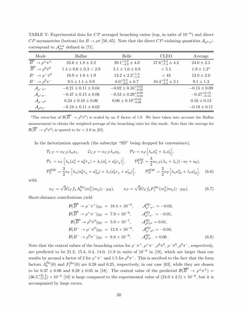
TABLE V: Experimental data for CP averaged branching ratios (top, in units of 10−6) and direct

CP asymmetries (bottom) for B → ρπ [50, 65]. Note that the direct CP -violating quantities Aρ±π∓

correspond to A∓±ρπ defined in [71].

Mode BaBar Belle CLEO Average

B0 → ρ±π∓ 22.6 ± 1.8± 2.2 29.1+5.0

−4.9 ± 4.0 27.6+8.4−7.4 ± 4.2 24.0 ± 2.5

B0 → ρ0π0 1.4± 0.6 ± 0.3 < 2.9 5.1 ± 1.6± 0.8 < 5.5 1.9± 1.2a

B− → ρ−π0 10.9 ± 1.9± 1.9 13.2± 2.3+1.4−1.9 < 43 12.0 ± 2.0

B− → ρ0π− 9.5± 1.1± 0.9 8.0+2.3−2.0 ± 0.7 10.4+3.3

−3.4 ± 2.1 9.1 ± 1.3

Aρ−π+ −0.21 ± 0.11± 0.04 −0.02± 0.16+0.05−0.02 −0.15 ± 0.09

Aρ+π− −0.47 ± 0.15± 0.06 −0.53± 0.29+0.09−0.04 −0.47+0.13

−0.14

Aρ−π0 0.24± 0.16 ± 0.06 0.06 ± 0.19+0.04−0.06 0.16 ± 0.13

Aρ0π− −0.19 ± 0.11± 0.02 −0.19 ± 0.11

aThe error-bar of B(B0 → ρ0π0) is scaled by an S factor of 1.9. We have taken into account the BaBar

measurement to obtain the weighted average of the branching ratio for this mode. Note that the average for

B(B0 → ρ0π0) is quoted to be < 2.9 in [65].

In the factorization approach (the subscript “SD” being dropped for convenience),

TV,P = κV,Pλua1, CV,P = κV,Pλua2, PP = κP[

λuau4 + λca

c4

]

,

PV = κV[

λu(au4 + au6rχ) + λc(a

c4 + ac6rχ)

]

, PEWV,P =

3

2κV,P (λu + λc)(−a7 + a9),

P ′EWV =

3

2κV[

λu(au8rχ + au10) + λc(a

c8rχ + ac10)

]

, P ′EWP =

3

2κP[

λuau10 + λca

c10

]

, (6.6)

with

κV =√2GF fπA

Bρ0 (m2

π)mρ(ε · pB), κP =√2GF fρF

Bπ1 (m2

ρ)mρ(ε · pB), (6.7)

Short-distance contributions yield

B(B0 → ρ−π+)SD = 18.4 × 10−6, ASDρ−π+ = −0.03,

B(B0 → ρ+π−)SD = 7.9 × 10−6, ASDρ+π− = −0.01,

B(B0 → ρ0π0)SD = 5.9 × 10−7, ASDρ0π0 = 0.01,

B(B− → ρ−π0)SD = 12.8 × 10−6, ASDρ−π0 = −0.04,

B(B− → ρ0π−)SD = 6.8 × 10−6, ASDρ0π− = 0.06 . (6.8)

Note that the central values of the branching ratios for ρ−π+, ρ+π−, ρ0π0, ρ−π0, ρ0π−, respectively,

are predicted to be 21.2, 15.4, 0.4, 14.0, 11.9 in units of 10−6 in [18], which are larger than our

results by around a factor of 2 for ρ+π− and 1.5 for ρ0π−. This is ascribed to the fact that the form

factors ABρ0 (0) and FBπ1 (0) are 0.28 and 0.25, respectively, in our case [63], while they are chosen

to be 0.37 ± 0.06 and 0.28 ± 0.05 in [18]. The central value of the predicted B(B0 → ρ±π∓) =

(36.5+21.4−17.6)× 10−6 [18] is large compared to the experimental value of (24.0± 2.5)× 10−6, but it is

accompanied by large errors.

30

��✒

��

❅❅❘

❅❅

❄

✲

✲

B

π

ρ

π

ρ

π

(a)

��✒

��

❅❅❘

❅❅

❄

✲

✲

B

D

D∗

D

ρ

π

(b)

��✒

��

❅❅❘

❅❅

❄

✲

✲

B

D

D∗

D∗

ρ

π

(c)

FIG. 8: Long-distance t-channel rescattering contributions to B → ρπ.

The long-distance contributions are depicted in Fig. 8:

Abs(8a) =GF√2λu

∫ 1

−1

|~p1|d cos θ16πmB

8g2ρππF 2(t,mπ)

t−m2π

mρ

[

afπABρ0 (m2

π) + bfρFBπ1 (m2

ρ)]

×(

−p2 · p3 +(p1 · p2)(p1 · p3)

m2ρ

)

E2|~p4| − E4|~p2| cos θmB |~p4|

,

Abs(8b) =GF√2λu

∫ 1

−1

|~p1|d cos θ16πmB

2√2 gD∗Dπ gV β

F 2(t,mD)

t−m2D

mD∗

×[

cfDABD∗

0 (m2D) + d fD∗FBD1 (m2

D∗)]

×(

−p2 · p3 +(p1 · p2)(p1 · p3)

m2ρ

)

E2|~p4| − E4|~p2| cos θmB |~p4|

,

Abs(8c) =GF√2λu

∫ 1

−1

|~p1|d cos θ16πmB

4√2 g2D∗Dπ gV λ

F 2(t,mD∗)

t−m2D∗

mD∗

×[

cfDABD∗

0 (m2D) + d fD∗FBD1 (m2

D∗)]

(

m24p1 · p2 − (p2 · p4)(p1 · p4)

+E1|~p4|+E4|~p1| cos θ

mB |~p4|[

(pB · p2)(p3 · p4)− (pB · p4)(p2 · p3)]

)

, (6.9)

where a = b = 1/2 for ρ0π0, a = 1 (1/√2), b = 0 for ρ−π+ (ρ0π−), a = 0, b = 1 (1/

√2) for

ρ+π− (ρ−π0), c = d = 1/2 for ρ0π0, c = d = 1/√2 for ρ0π−, c = d = −1/

√2 for ρ−π0, c = 1, d = 0

for ρ−π+, and c = 0, d = 1 for ρ+π−.

A χ2 fit of the cutoff scales Λπ,ΛD(∗) or the cutoff parameters ηπ and ηD(∗)to the measured

branching ratios of B → ρπ shows a flat χ2 without a minimum for ηD <∼ 2. Therefore, we choose

the criterion that FSI contributions should accommodate the data of the ρ0π0 and ρ0π− without

affecting ρ±π∓ and ρ−π0 significantly. Using ηD = ηD∗ = 1.6 , the branching ratios and direct

CP asymmetries after taking into account long-distance rescattering effects are shown in Table VI.

(The results are rather insensitive to ηπ.) We see that, in contrast to the πK case, the B → ρπ

decays are less sensitive to the cutoff scales. The B0 → ρ0π0 rate is enhanced via rescattering

by a factor of 2, which is consistent with the weighted average of (1.9 ± 1.2) × 10−6. However, it

is important to clarify the discrepancy between BaBar and Belle measurements for this mode. It

should be remarked that direct CP violation in this mode is significantly enhanced by FSI from

around 1% to 60%. Naively, this asymmetry ought to become accessible at B factories with 108

BB pairs. As stressed before, there is 3.6σ direct CP violation in the ρ+π− mode. Our prediction

31

TABLE VI: Same as Table II except for B → ρπ decays.

Mode Expt. SD SD+LD

B(B0 → ρ−π+) 13.9+2.2−2.1 18.4 18.8+0.3

−0.2

B(B0 → ρ+π−) 10.1+2.1−1.9 7.9 8.4± 0.3

B(B0 → ρ±π∓) 24.0 ± 2.5 26.3 27.3+0.6−0.4

B(B0 → ρ0π0) 1.9 ± 1.2 0.6 1.3+0.4−0.3

B(B− → ρ−π0) 12.0 ± 2.0 12.9 14.0+0.7−0.4

B(B− → ρ0π−) 9.1 ± 1.3 6.8 7.5+0.6−0.3

Aρ−π+ −0.15± 0.09 −0.03 −0.24± 0.6

Aρ+π− −0.47+0.13−0.14 −0.01 −0.43 ± 0.11

Aρ0π0 0.01 0.57+0.01−0.03

Aρ−π0 0.16 ± 0.13 −0.04 0.36 ± 0.10

Aρ0π− −0.19± 0.11 0.06 −0.56+0.14−0.15

of Aρ+π− agrees with the data in both magnitude and sign, while the QCD factorization prediction

(0.6+11.6−11.8)% [18] seems not consistent with experiment.

VII. POLARIZATION IN B → φK∗, ρK∗ DECAYS

The branching ratios and polarization fractions of charmless B → V V decays have been mea-

sured for ρρ, ρK∗ and φK∗ final states. In general, it is expected that they are dominated by the

longitudinal polarization states and respect the scaling law, namely [26] (see also footnote 1 on p.3)

1− fL = O(m2V /m

2B), f⊥/f‖ = 1 +O(mV /mB) (7.1)

with fL, f⊥ and f‖ being the longitudinal, perpendicular, and parallel polarization fractions, re-

spectively. However, in sharp contrast to the ρρ case, the large fraction of transverse polarization

in B → φK∗ decays observed by BaBar and confirmed by Belle (see Table VII) is a surprise and

poses an interesting challenge for any theoretical interpretation. The aforementioned scaling law

remains true even when nonfactorizable graphs are included in QCD factorization [26]. Therefore,

in order to obtain a large transverse polarization in B → φK∗, this scaling law valid at short-

distance interactions must be circumvented in one way or another. One way is the Kagan’s recent

suggestion of sizable penguin-induced annihilation contributions [27]. Another possibility is that

perhaps a sizable transverse polarization can be achieved via final-state rescattering. To be more

specific, the following two FSI processes are potentially important. First, B → D∗D∗s followed by a

rescattering to φK∗ is not subject to the scaling law and hence its large transverse polarization can

be conveyed to φK∗ via FSI. Second, the FSI effect from B → D∗Ds or B → DD∗s will contribute

only to the A⊥ amplitude. In this section, we shall carefully examine the long-distance rescattering

effects on φK∗ polarizations.

32

TABLE VII: Experimental data for CP averaged branching ratios (in units of 10−6) and polariza-

tion fractions for B → φK∗, ρK∗, ρρ [50, 65, 74, 75]. The phases of the parallel and perpendicular

amplitudes relative to the longitudinal one for B → φK∗ are also included [74, 75].

Mode BaBar Belle CLEO Average

B0 → φK

∗09.2 ± 0.9± 0.5 10.0+1.6+0.7

−1.5−0.8 11.5+4.5+1.8−3.7−1.7 9.5 ± 0.9

B− → φK∗− 12.7+2.2−2.0 ± 1.1 6.7+2.1+0.7

−1.9−1.0 10.6+6.4+1.8−4.9−1.6 9.7 ± 1.5

B0 → ρ+K∗− 16.3 ± 5.4± 2.3+0.0

−6.3 < 24 < 24

B− → ρ0K∗− 10.6+3.0−2.6 ± 2.4 < 74 10.6+3.8

−3.5

B− → ρ−K∗0

17.0 ± 2.9± 2.0+0.0−1.9 6.6± 2.2 ± 0.8 9.6± 4.7a

B− → ρ0ρ− 22.5+5.7−5.4 ± 5.8 31.7 ± 7.1+3.8

−6.7 26.4+6.1−6.4

B0 → ρ+ρ− 30± 4± 5 30± 6

B− → ρ−ω 12.6+3.7−3.3 ± 1.8 12.6+4.1

−3.8

fL(φK∗0) 0.52 ± 0.05 ± 0.02 0.52 ± 0.07 ± 0.05 0.52 ± 0.05

f⊥(φK∗0) 0.22 ± 0.05 ± 0.02 0.30 ± 0.07 ± 0.03 0.25 ± 0.04

fL(φK∗−) 0.46 ± 0.12 ± 0.03 0.49 ± 0.13 ± 0.05 0.47 ± 0.09

f⊥(φK∗−) 0.12+0.11−0.08 ± 0.03 0.12+0.11

−0.09

φ‖(φK∗0) (rad)b 2.34+0.23

−0.20 ± 0.05 −2.30 ± 0.28 ± 0.04

φ⊥(φK∗0) (rad)b 2.47 ± 0.25 ± 0.05 0.64 ± 0.26 ± 0.05

φ‖(φK∗+) (rad)b −2.07 ± 0.34 ± 0.07 −2.07 ± 0.35

φ⊥(φK∗+) (rad)b 0.93+0.55−0.39 ± 0.12 0.93+0.56

−0.41

fL(ρ0K∗−) 0.96+0.04

−0.15 ± 0.04 0.96+0.06−0.16

fL(ρ−K

∗0) 0.79 ± 0.08± 0.04 ± 0.02 0.50 ± 0.19+0.05

−0.07 0.74 ± 0.08

fL(ρ0ρ−) 0.97+0.03

−0.07 ± 0.04 0.95 ± 0.11 ± 0.02 0.96+0.04−0.07

fL(ρ+ρ−) 0.99 ± 0.03 ± 0.04 0.99 ± 0.05

fL(ρ−ω) 0.88+0.12

−0.15 ± 0.03 0.88+0.12−0.15

aThe error in B(B− → ρ−K∗0) is scaled by S = 2.4. Our average is slightly different from the value of

9.2± 2.0 quoted in [65].bExperimental results of the relative strong phases are for B(0,+) → φK∗(0,+) decays.

A. Short-distance contributions to B → φK∗

In the factorization approach, the amplitude of the B → φK∗ decay is given by

〈φ(λφ)K∗(λK∗)|Heff |B〉 =GF√2

∑

q=u,c

VqbV∗qs a

qφK∗ 〈φ|(ss)V |0〉 〈K∗|(sb)V−A|B〉

= −iαφK∗ ε∗µφ (λφ)ε∗νK∗(λK∗)

(

ABK∗

1 (m2φ)gµν

−2ABK

∗

2 (m2φ)

(mB +mK∗)2pBµpBν − i

2V BK∗(m2

φ)

(mB +mK∗)2ǫµναβp

αBp

βK∗

)

, (7.2)

33

where λφ,K∗ are the corresponding helicities, aqφK∗ ≡ a3 + aq4 + a5 − (a7 + a9 + aq10)/2 and

αφK∗ ≡ GFmφfφ(mB + mK∗)∑

q=u,c VqbV∗qs a

qφK∗/

√2. With Aλ defined as 〈φ(λ)K∗(λ)|Heff |B〉,

it is straightforward to obtain [76]

A0 = −iαφK∗

(

−ABK∗

1 (m2φ)m2B −m2

φ −m2K∗

2mφmK∗+

2ABK∗

2 (m2φ)

(mB +mK∗)2m2Bp

2c

mφmK∗

)

,

A± = −iαφK∗

(

ABK∗

1 (m2φ)∓

2V BK∗(m2

φ)

(mB +mK∗)2mBpc

)

, (7.3)

where pc is the center of mass momentum and we have used the phase convention εφ(λ) = εK∗(−λ)for ~pφ,K∗ → 0. The longitudinal amplitude A0 is sometimes denoted as AL, while the transverse

amplitudes are defined by

A‖ =A+ +A−√

2= −iαφK∗

√2ABK

∗

1 (m2φ),

A⊥ =A+ −A−√

2= iαφK∗

2√2V BK∗

(m2φ)

(mB +mK∗)2mBpc (7.4)

in the transversity basis. The decay rate can be expressed in terms of these amplitudes as

Γ =pc

8πm2B

(|A0|2 + |A+|2 + |A−|2) =pc

8πm2B

(|AL|2 + |A‖|2 + |A⊥|2), (7.5)

and the polarization fractions are defined as

fα ≡ ΓαΓ

=|Aα|2

|A0|2 + |A‖|2 + |A⊥|2, (7.6)

with α = L, ‖,⊥.

The form factors A1, A2, V usually are similar in size [63]. Using above equations with ai

given in (4.6) 14 and the form factors given in [63], one immediately finds that the short-distance

contributions yield (see also Table VIII)

fSDL : fSD‖ : fSD⊥ = 0.88 ± 0.06 : 0.07 ± 0.03 : 0.05 ± 0.03, 1 ≃ fSDL ≫ fSD‖,⊥, (7.7)

where the errors are estimated with 10% uncertainties in form factors. However, the above pre-

diction is not borne out by the B → φK∗ data (see Table VII). It is easily seen that Eq. (7.7) is

closely related to the fact that mB ≫ mφ,K∗. We do not expect that such a relation holds in the

case of B → D(∗)D(∗)s decays, which can rescatter to the φK∗ final state. It is thus interesting to

investigate the effect of FSI on these polarization fractions. A similar analysis was also considered

recently in [78].

Another possible shortcoming of the short-distance factorization approach is that the central

value of the predicted branching ratio

B(B → φK∗)SD = (4.4 ± 2.6)× 10−6 (7.8)

14 As shown explicitly in [77] within the QCD factorization approach, nonfactorizable corrections to each

partial-wave or helicity amplitude are in general not the same; the effective parameters ai can vary for

different helicity amplitudes. However, since such an effect is too small to account for the large transverse

polarization [26], for simplicity we shall ignore the difference of ai in different helicity amplitudes.

34

D(∗)s

(k)

D(∗)(p2)

D(∗)s

(p1)

K∗(p4)

φ(p3)

B

FIG. 9: Long-distance t-channel rescattering contributions to B → φK∗. Note that flows in lines

are along b or c quarks.

is too small by a factor of 2 compared to experiment. As pointed out in [77], in the heavy quark

limit, both vector mesons in the charmless B → V V decays should have zero helicity and the

corresponding amplitude is governed by the form factor A0. Consequently, the predicted branching

ratios are rather sensitive to the form factor models of A0 and can be easily different by a factor

of 2. Using the covariant light-front model for B → K∗ form factors [63], we are led to the above

prediction in Eq. (7.8). A similar result is also obtained in the BSW model [77]. However, a much

larger branching ratio will be obtained if the form factors based on light-cone sum rules [79, 80]

are employed. At any rate, if the predicted rate is too small, this is another important incentive

for considering long-distance effects.

B. Long-distance contributions to B → φK∗

The D(∗)D(∗)s states from B decays can rescatter to φK∗ through the t-channel D

(∗)s exchange in

the triangle diagrams depicted in Fig. 9. The effective Lagrangian for D(∗)D(∗)V vertices is given

in Eq. (3.15). Note that as in Eq. (4.12), SU(3) or U(3) breaking effects in strong couplings are

assumed to be taken into account by the relations

gD(∗)D

(∗)s K∗ =

√

mD

(∗)s

mD(∗)

gD(∗)D(∗)ρ, gD

(∗)s D

(∗)s φ

=mD

(∗)s

mD(∗)

gD(∗)D(∗)ρ, (7.9)

and likewise for fD(∗)D

(∗)s K∗ and f

D(∗)s D

(∗)s φ

.

There are totally eight different FSI diagrams in Fig. 9. The absorptive part contribution of

B → DsD → φK∗amplitude via the Ds exchange is given by

Abs (DsD;Ds) =1

2

∫

d3~p1(2π)32E1

d3~p2(2π)32E2

(2π)4δ4(pB − p1 − p2)A(B0 → DsD)

×(2i)gDsDsφF 2(t,mDs

)

t−m2Ds

(−2i)gDDsK∗ (ε∗3 · p1)(ε∗4 · p2). (7.10)

We need to use some identities to recast the above amplitude into the standard expression given in

Eq. (7.2). To proceed, we note that after performing the integration, the integrals

∫

d3~p1(2π)32E1

d3~p2(2π)32E2

(2π)4δ4(pB − p1 − p2)f(t)× {p1µ, p1µp1ν , p1µp1νp1α} (7.11)

35

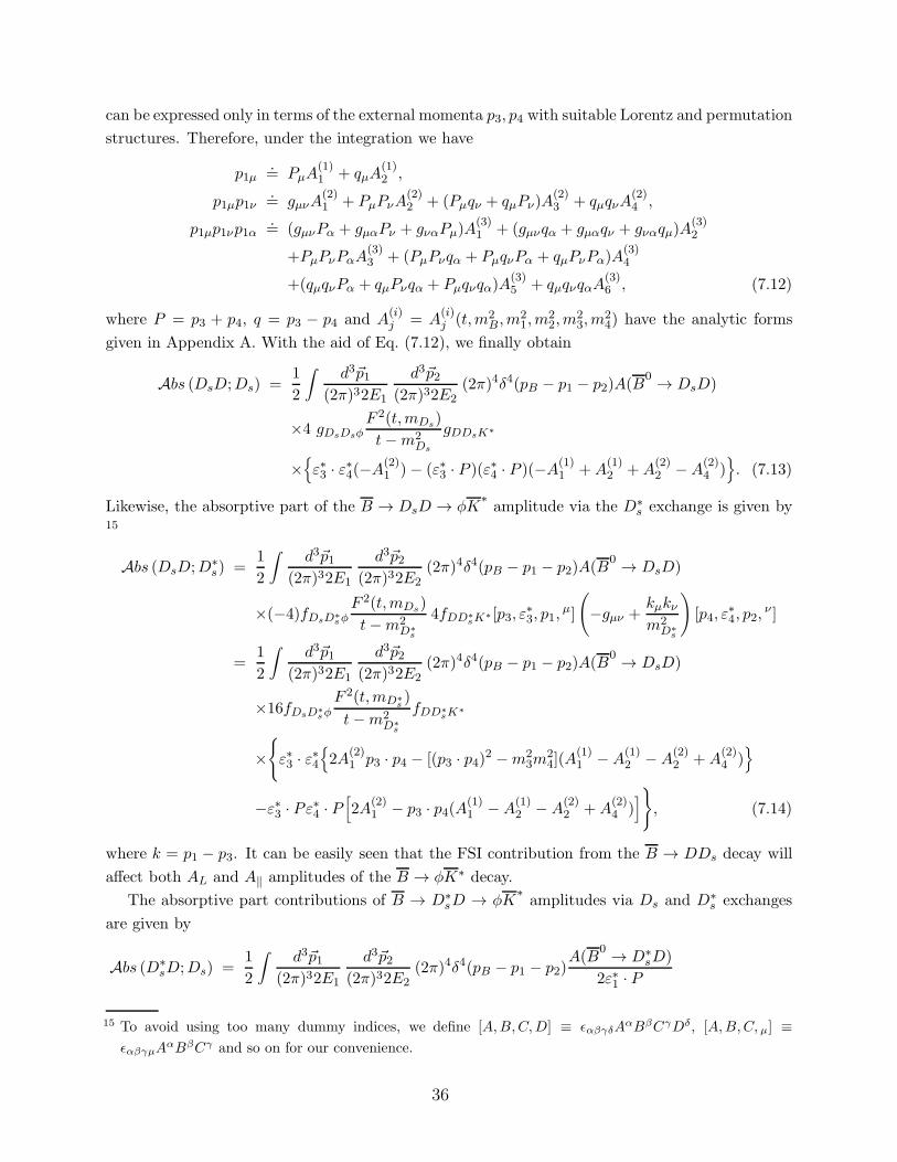
can be expressed only in terms of the external momenta p3, p4 with suitable Lorentz and permutation

structures. Therefore, under the integration we have

p1µ.= PµA

(1)1 + qµA

(1)2 ,

p1µp1ν.= gµνA

(2)1 + PµPνA

(2)2 + (Pµqν + qµPν)A

(2)3 + qµqνA

(2)4 ,

p1µp1νp1α.= (gµνPα + gµαPν + gναPµ)A

(3)1 + (gµνqα + gµαqν + gναqµ)A

(3)2

+PµPνPαA(3)3 + (PµPνqα + PµqνPα + qµPνPα)A

(3)4

+(qµqνPα + qµPνqα + Pµqνqα)A(3)5 + qµqνqαA

(3)6 , (7.12)

where P = p3 + p4, q = p3 − p4 and A(i)j = A

(i)j (t,m2

B ,m21,m

22,m

23,m

24) have the analytic forms

given in Appendix A. With the aid of Eq. (7.12), we finally obtain

Abs (DsD;Ds) =1

2

∫

d3~p1(2π)32E1

d3~p2(2π)32E2

(2π)4δ4(pB − p1 − p2)A(B0 → DsD)

×4 gDsDsφF 2(t,mDs

)

t−m2Ds

gDDsK∗

×{

ε∗3 · ε∗4(−A(2)1 )− (ε∗3 · P )(ε∗4 · P )(−A

(1)1 +A

(1)2 +A

(2)2 −A

(2)4 )}

. (7.13)

Likewise, the absorptive part of the B → DsD → φK∗amplitude via the D∗

s exchange is given by15

Abs (DsD;D∗s) =

1

2

∫

d3~p1(2π)32E1

d3~p2(2π)32E2

(2π)4δ4(pB − p1 − p2)A(B0 → DsD)

×(−4)fDsD∗sφF 2(t,mDs

)

t−m2D∗

s

4fDD∗sK

∗ [p3, ε∗3, p1,

µ]

(

−gµν +kµkνm2D∗

s

)

[p4, ε∗4, p2,

ν ]

=1

2

∫

d3~p1(2π)32E1

d3~p2(2π)32E2

(2π)4δ4(pB − p1 − p2)A(B0 → DsD)

×16fDsD∗sφF 2(t,mD∗

s)

t−m2D∗

s

fDD∗sK

∗

×{

ε∗3 · ε∗4{

2A(2)1 p3 · p4 − [(p3 · p4)2 −m2

3m24](A

(1)1 −A

(1)2 −A

(2)2 +A

(2)4 )}

−ε∗3 · Pε∗4 · P[

2A(2)1 − p3 · p4(A(1)

1 −A(1)2 −A

(2)2 +A

(2)4 )]

}

, (7.14)

where k = p1 − p3. It can be easily seen that the FSI contribution from the B → DDs decay will

affect both AL and A‖ amplitudes of the B → φK∗ decay.

The absorptive part contributions of B → D∗sD → φK

∗amplitudes via Ds and D∗

s exchanges

are given by

Abs (D∗sD;Ds) =

1

2

∫

d3~p1(2π)32E1

d3~p2(2π)32E2

(2π)4δ4(pB − p1 − p2)A(B

0 → D∗sD)

2ε∗1 · P

15 To avoid using too many dummy indices, we define [A,B,C,D] ≡ ǫαβγδAαBβCγDδ, [A,B,C, µ] ≡

ǫαβγµAαBβCγ and so on for our convenience.

36

×∑

λ1

2ε∗1 · P (−4i)fD∗sDsφ

F 2(t,mDs)

t−m2Ds

(−2i)gDDsK∗ [p3, ε∗3, p1, ε1]p2 · ε∗4

=1

2

∫

d3~p1(2π)32E1

d3~p2(2π)32E2

(2π)4δ4(pB − p1 − p2)A(B

0 → D∗sD)

2ε∗1 · P

×(−i)[ε∗3, ε∗4, p3, p4]{

− 16i fD∗sDsφ

F 2(t,mDs)

t−m2Ds

gDDsK∗ A(2)1

}

,

Abs (D∗sD;D∗

s) =1

2

∫

d3~p1(2π)32E1

d3~p2(2π)32E2

(2π)4δ4(pB − p1 − p2)A(B

0 → D∗sD)

2ε∗1 · P

×∑

λ1

2ε∗1 · P (−4i)fD∗sD

∗sφF 2(t,mD∗

s)

t−m2D∗

s

4i fDD∗sK

∗

×ερ1(σgρµp1 · ε∗3 + p3ρε∗3µ − ε∗3ρp3µ)

(

− gµν +kµkν

m2D∗

s

)

[p4, ε∗4, p2,

ν ]

=1

2

∫

d3~p1(2π)32E1

d3~p2(2π)32E2

(2π)4δ4(pB − p1 − p2)A(B

0 → D∗sD)

2ε∗1 · P

×(−i)[ε∗3, ε∗4, p3, p4] (−32i) fD∗sD

∗sφF 2(t,mD∗

s)

t−m2D∗

s

fDD∗sK

∗

{

A(2)1

[

σ + (1− σ)P · p1m2

1

]

+(1−A(1)1 −A

(1)2 )

(

P · p3 −P · p1p1 · p3

m21

)}

, (7.15)

where the dependence of the polarization vector in A(B0 → D∗

sD) has been extracted out explicitly

and σ ≡ gD∗D∗V /(2fD∗D∗V ).

Similarly, the absorptive parts of B → DsD∗ → φK

∗amplitudes via Ds and D∗

s exchanges are

given by

Abs (DsD∗;Ds) =

1

2

∫

d3~p1(2π)32E1

d3~p2(2π)32E2

(2π)4δ4(pB − p1 − p2)A(B

0 → DsD∗)

2ε∗2 · P

×∑

λ2

2ε∗2 · P 2igDsDsφF 2(t,mDs

)

t−m2Ds

(−4i)fD∗DsK∗ [p4, ε∗4, p2, ε2]p1 · ε∗3

=1

2

∫

d3~p1(2π)32E1

d3~p2(2π)32E2

(2π)4δ4(pB − p1 − p2)A(B

0 → DsD∗)

2ε∗2 · P

×(−i)[ε∗3, ε∗4, p3, p4]{

16i gDsDsφF 2(t,mDs

)

t−m2Ds

fD∗DsK∗ A(2)1

}

,

Abs (DsD∗;D∗

s) =1

2

∫

d3~p1(2π)32E1

d3~p2(2π)32E2

(2π)4δ4(pB − p1 − p2)A(B

0 → DsD∗)

2ε∗2 · P

×∑

λ2

2ε∗2 · P 4i fDsD∗sφF 2(t,mD∗

s)

t−m2D∗

s

(4i)fD∗D∗sK

∗

×[p3, ε∗3, p1, µ]

(

− gµν +kµkν

m2D∗

s

)

(σgναp2 · ε∗4 − p4νε∗4α + ε∗4νp4α)ε

α2

=1

2

∫

d3~p1(2π)32E1

d3~p2(2π)32E2

(2π)4δ4(pB − p1 − p2)A(B

0 → DsD∗)

2ε∗2 · P

37

×(−i)[ε∗3, ε∗4, p3, p4] 32i fDsD∗sφF 2(t,mD∗

s)

t−m2D∗

s

fD∗D∗sK

∗

{

A(2)1

[

σ + (1− σ)P · p2m2

2

]

+(A(1)1 −A

(1)2 )

(

P · p4 −P · p2p2 · p4

m22

)}

, (7.16)

where again the dependence of the polarization vector in A(B0 → DsD

∗) has been extracted out

explicitly. Note that through rescattering FSI, both B → D∗sD and B → DsD

∗ will affect only the

A⊥ term of the B → φK∗ decay amplitude.

To consider the FSI effect from the decay B → D∗sD

∗, we denote the decay amplitude as

A(B → D∗s(p1, λ1)D

∗(p2, λ2)) = ε∗µ1 ε∗ν2 (a gµν + bPµPν + ic [µ, ν , P, p2]). (7.17)

The absorptive part of the B → D∗sD

∗ → φK∗amplitude via a t-channel Ds exchange has the

expression

Abs (D∗sD

∗;Ds) =1

2

∫

d3~p1(2π)32E1

d3~p2(2π)32E2

(2π)4δ4(pB − p1 − p2)(a gµν + bPµPν + ic[µ, ν , P, p2])

×∑

λ1,λ2

ε∗µ1 ε∗ν2 (−4i)fD∗sDsφ

F 2(t,mDs)

t−m2Ds

(−4i)fD∗DsK∗ [p3, ε∗3, p1, ε1][p4, ε

∗4, p2, ε2]

=1

2

∫

d3~p1(2π)32E1

d3~p2(2π)32E2

(2π)4δ4(pB − p1 − p2)16fD∗sDsφ

F 2(t,mDs)

t−m2Ds

fD∗DsK∗

×{

ε∗3 · ε∗4{2a p3 · p4A(2)1 − [(p3 · p4)2−m2

3m24][a(A

(1)1 −A

(1)2 −A

(2)2 +A

(2)4 ) + bA

(2)1 ]}

−ε∗3 · Pε∗4 · P{2aA(2)1 − p3 · p4[a(A(1)

1 −A(1)2 −A

(2)2 +A

(2)4 ) + bA

(2)1 ]}

−i[ε∗3, ε∗4, p3, p4] 2c{

P · p3(A(2)1 −A

(3)1 −A

(3)2 ) + P · p4(A(3)

1 −A(3)2 )− p3 · p4A(3)

2

+[(p3 · p4)2 −m23m

24](A

(2)3 −A

(2)4 −A

(3)4 +A

(3)6 )}

}

. (7.18)

We see that the above FSI contributes to all three polarization components. The contribution from

the D∗s exchange is

Abs (D∗sD

∗;D∗s) =

1

2

∫

d3~p1(2π)32E1

d3~p2(2π)32E2

(2π)4δ4(pB − p1 − p2)(a gδβ + bPδPβ + ic[δ , β, P, p2])

×∑

λ1,λ2

ε∗δ1 ε∗β2 (−4i)fD∗

sD∗sφF 2(t,mD∗

s)

t−m2D∗

s

(4i)fD∗D∗sK

∗ ερ1(σgρµp1 · ε∗3+ p3ρε∗3µ− ε∗3ρp3µ)

×(

− gµν +kµkν

m2D∗

s

)

(σgναp2 · ε∗4 − p4νε∗4α + ε∗3νp3α)ε

α2

=1

2

∫

d3~p1(2π)32E1

d3~p2(2π)32E2

(2π)4δ4(pB − p1 − p2) 16fD∗sD

∗sφF 2(t,mD∗

s)

t−m2D∗

s

fD∗D∗sK

∗

×{

ε∗3 · ε∗4{[

− 1 +(1− σ)2

m2D∗

s

A(2)1

][

a p3 · p4 + bp3 · p2p1 · p4

+a+ bp1 · p2m2

1m22

(−m22p3 · p1p1 · p4 −m2

1p3 · p2p2 · p4 + p3 · p1p1 · p2p2 · p4)]

+a

(

− p3 · p4 +p3 · kk · p4m2D∗

s

)

+A(2)1

{

σ2[

2a− bp1 · p2 +a+ bp1 · p2m2

1m22

(p1 · p2)2]

38

+σ

[

b− a+ bp1 · p2m2

1m22

p1 · p2]

P 2

+(σ − 1)p4 · km2D∗

s

[

bp2 · p3 +a+ bp1 · p2m2

1m22

(m21p2 · p3 −m2

2p1 · p3 − p2 · p1p1 · p3)]

+(σ − 1)p3 · km2D∗

s

[

− bp1 · p4 +a+ bp1 · p2m2

1m22

(m21p2 · p4 −m2

2p1 · p4 + p1 · p2p2 · p4)]

+

(

p3 · p4 −p3 · kk · p4m2D∗

s

)[

b+a+ bp1 · p2m2

1m22

(m21 +m2

2 + p1 · p2)]}}

−ε∗3 · Pε∗4 · P{

(1− σ)2

m2D∗

s

(A(1)1 −A

(1)2 −A

(2)2 +A

(2)4 )

[

a p3 · p4 + bp3 · p2p1 · p4

+a+ bp1 · p2m2

1m22

(−m22p3 · p1p1 · p4 −m2

1p3 · p2p2 · p4 + p3 · p1p1 · p2p2 · p4)]

+σ2(A(1)1 −A

(1)2 −A

(2)2 +A

(2)4 )

[

2a− bp1 · p2 +(p1 · p2)2m2

1m22

(a+ bp1 · p2)]

−σ[

b− a+ bp1 · p2m2

1m22

p1 · p2]

[(A(2)2 −A

(2)4 )P 2 + (1− 2A

(1)1 )p1 · p3

−(A(1)1 −A

(1)2 )(p1 · p4 + p2 · p3)]−

[

1− (1− σ)(A(1)1 −A

(1)2 )

p4 · km2D∗

s

]

×[

a+a+ bp1 · p2m2

1m22

(−m21p2 · p3 + p2 · p1p1 · p3)

]

−[

1 + (1− σ)(1−A(1)1 −A

(1)2 )

p3 · km2D∗

s

](

a+ bp1 · p4 −a+ bp1 · p2

m22

p2 · p4)

−[

A(1)1 +A

(1)2 − (1− σ)(A

(2)2 −A

(2)4 )

p4 · km2D∗

s

]

×[

bp2 · p3 +a+ bp1 · p2m2

1m22

(m21p2 · p3 −m2

2p1 · p3 − p2 · p1p1 · p3)]

+

[

A(1)1 −A

(1)2 + (1− σ)

p3 · km2D∗

s

(A(1)1 −A

(1)2 −A

(2)2 +A

(2)4 )

)

×[

bp1 · p4 −a+ bp1 · p2m2

1m22

(m21p2 · p4 −m2

2p1 · p4 + p1 · p2p2 · p4)]

+

(

p3 · p4 −p3 · kk · p4m2D∗

s

)

{

b(A(1)1 +A

(1)2 −A

(2)2 +A

(2)4 )

+a+ bp1 · p2m2

1m22

[p1 · p2(A(1)1 −A

(1)2 −A

(2)2 +A

(2)4 )−m2

1(1− 2A(1)1 +A

(2)2 −A

(2)4 )

−m22(A

(2)2 −A

(2)4 )]

}

}

− i[ε∗3, ε∗4, p3, p4] 2c

{(

p3 · p4 −p3 · kk · p4m2D∗

s

)

A(1)2

−[

2σ − (1− σ)q · k2m2

D∗s

]

A(2)1

}

}

, (7.19)

with P = p3 + p4, q = p3 − p4 and k = p1 − p3 = p4 − p2 as before. Clearly the above rescattering

amplitude contributes to all three polarization components AL,‖,⊥.

39

C. Numerical results

In order to perform a numerical study of the analytic results obtained in the previous subsection,

we need to specify the short-distance A(B → D(∗)s D(∗)) amplitudes. In the factorization approach,

we have

A(B → DsD)SD = iGF√2VcbV

∗csa1fDs

(m2B −m2

D)FBD0 (m2

Ds),

A(B → D∗sD)SD =

GF√2VcbV

∗csa1fD∗

smD∗

sFBD1 (m2

D∗s)(2ε∗D∗

s· pB),

A(B → DsD∗)SD =

GF√2VcbV

∗csa1fDs

mD∗ABD∗

0 (m2Ds

)(2ε∗D∗ · pB),

A(B → D∗sD

∗)SD = −iGF√2VcbV

∗csa1fD∗

smD∗

s(mB +mD∗)ε∗µD∗

sε∗νD∗

[

ABD∗

1 (m2D∗

s)gµν

−2ABD

∗

2 (m2D∗

s)

(mB +mD∗)2pBµpBν − i

2V BD∗(m2

D∗s)

(mB +mD∗)2ǫµναβp

αBp

βD∗

]

. (7.20)

Writing A = ASD + iAbsALD with AbsALD being given in the previous subsection and using the

form factors given in [63], we obtain the numerical results for B → φK∗ amplitudes as exhibited

in Table VIII. The branching ratio after the inclusion of FSIs is

B(B → φK∗) = (9.2+4.3−2.7)× 10−6 (7.21)

for ΛDs,D∗s= mDs,D∗

s+ηΛQCD with η = 0.80 and 15% error in ΛQCD. Several remarks are in order.

(i) The polarization amplitudes are very sensitive to the cutoffs ΛDs,D∗s. (ii) We have assumed a

monopole behavior [i.e. n = 1 in Eq. (3.22)] for the form factor F (t,mDs) and a dipole form

(i.e. n = 2) for F (t,mD∗s).16 If the monopole form for F (t,mD∗

s) is utilized, the parameter η

will become unnaturally small in order to avoid too large FSI contributions. (iii) the interference

between short-distance and long-distance contributions is mild. This is because B → φK∗ and

B → D(∗)s D(∗) amplitudes should have the similar weak phase as |VcbV ∗

cs| ≫ |VubV ∗us|. 17 As a

result, the long-distance contribution is essentially “orthogonal” to the short-distance one. (iv)

The calculated strong phases shown in Table VIII are in agreement with experiment for φ‖ but not

16 For B → Dπ, Kπ, ππ decays, assuming a dipole form for the form factor appearing in the VexcV P or

VexcV V vertex with Vexc being the exchanged vector particle [see e.g. Figs. 4(e), 4(f), 5(d) and 6(e)] and a

monopole behavior for all other form factors, we found that the best χ2 fit to the measured decay rates is

very similar to the one with the monopole form for all the form factors. Only the cutoff Λ or the parameter

η appearing in Eq. (3.40) is slightly modified. The resultant branching ratios and CP asymmetries remain

almost the same. The same exercise also indicates that if the dipole behavior is assumed for all the form

factors, then the χ2 value becomes too poor to be acceptable. This is the another good reason why we

usually choose n = 1 in Eq. (3.22) for the form factors except for the one appearing in VexcV P or VexcV V

vertex.17 The weak phase of SD B → φK

∗and B → D

(∗)s D(∗) is not exactly the same. Moreover, our B → φK

∗

SD amplitude is not purely imaginary. It carries a phase as shown in Table VIII mainly because of the

phase difference in au4 and ac4 in our case [cf. Eq. (4.6)].

40

TABLE VIII: Short-distance (SD) and long-distance (LD) contributions to the decay amplitudes

(in unit of 10−8 GeV) and the polarization fractions for B → φK∗. LD contributions are calculated

with ΛDs,D∗s= mDs,D∗

s+ ηΛQCD, where η = 0.8 and errors come from a 15% variation on ΛQCD.

longitudinal (L) parallel (‖) perpendicular (⊥)

ASD 0.63− 1.98i −0.18 + 0.55i 0.15 − 0.46i

ASD+LD −0.57+0.33−0.39 − (2.03 ± 0.01)i 2.28+0.77

−0.67 + (0.64 ± 0.03)i 0.32± 0.05 − (0.44 ± 0.00)i

A(DsD;Ds) −1.10+0.30−0.34 − (0.04 ± 0.01)i 0.07 ± 0.02 + 0.00i 0

A(DsD;D∗s) 0.00 −0.02 ± 0.01− 0.00i 0

A(D∗sD;Ds) 0 0 −0.19 ± 0.05 − 0.01i

A(D∗sD;D∗

s) 0 0 −0.01 − 0.00i

A(DsD∗;Ds) 0 0 0.17 ± 0.05 + 0.01i

A(DsD∗;D∗

s) 0 0 0.01 + 0.00i

A(D∗sD

∗;Ds) −0.06± 0.02 − 0.00i 2.35+0.73−0.63 + (0.09+0.03

−0.02)i 0.21+0.07−0.06 + 0.01i

A(D∗sD

∗;D∗s) −0.04+0.02

−0.03 − 0.00i 0.06+0.04−0.03 + 0.00i −0.01 ± 0.01 − 0.00i

fSD 0.88 0.07 0.05

fSD+LD 0.43+0.13−0.09 0.54+0.10

−0.14 0.03 ± 0.01

f expt 0.51 ± 0.04 a 0.27 ± 0.06 a 0.22 ± 0.04 a

arg(AiA∗L)SD – π 0

arg(AiA∗L)SD+LD – 2.12+0.11

−0.07 0.89+0.21−0.24

arg(AiA∗L)

BaBar – 2.34+0.23−0.20 ± 0.05 −0.67 ± 0.25 ± 0.05 b

arg(AiA∗L)

Belle – 2.21± 0.22 ± 0.05 b −0.72 ± 0.21 ± 0.06 b

af expt is the experimental average of polarization fractions for B− → φK∗− and B0 → φK

∗0.

bSee footnote 18 for details.

for φ⊥.18 (v) There are large cancellations among various long-distance contributions, e.g. between

A(D∗sD;D

(∗)s ) and A(DsD

∗;D(∗)s ).

The cancellation in B → D∗sD → φK∗ and B → DsD

∗ → φK∗ contributions can be understood

from SU(3) symmetry, CP conjugation 19 and the similarity in the size of source amplitudes. To

see this, let 〈φ(ss)K∗(qs)|Tst|D∗s(cs)D(qc)〉 be the D∗

sD → φK∗ rescattering matrix element, which

is represented in the right-hand part of Fig. 9. After changing s → q in D∗s(cs) and φ(ss) (on

18 In Table VII, the experimental results of φ‖ and φ⊥ are for B → φK∗ decays. The Belle results for (φ‖, φ⊥)

should be transformed to (−φ‖, π − φ⊥). This phase transformation will not modify the experimentally

measured distributions (see [81] for details) but it will flip the relative sign between φ‖, φ⊥ and lead to

|A+| > |A−| for B → φK∗ as expected from the factorization approach. Since our calculations are for

B → φK∗decays, in Table VIII we have transformed BaBar and Belle results from φ⊥ to φ⊥ − π so that

|A+| < |A−| in B → φK∗. Note that in the absence of FSIs, φ‖ = φ⊥ = π for B → φK∗ and φ‖ = π,

φ⊥ = 0 for B → φK∗.

19 The combined symmetry is reminiscent of CPS symmetry which is used extensively in kaon decay matrix

elements on the lattice [82, 83].

41

the upper right part of Fig. 9), and q → s in D(qc) and K∗(qs) (on the lower right part of of

the same figure) under the SU(3) symmetry transformation, the above matrix element becomes

〈K∗(sq)φ(ss)|Tst|D∗(cq)Ds(sc)〉. Applying charge conjugation after the SU(3) transformation, we

are led to

〈φ(ss)K∗(qs)|Tst|D∗s(cs)D(qc)〉 = −〈K∗(qs)φ(ss)|Tst|D∗(qc)Ds(cs)〉, (7.22)

where the overall negative sign arises from the transformation of vector particles under charge con-

jugation. In the B → D∗sD → φK∗ rescattering amplitude, the above matrix element is sandwiched

by ε∗(p1, λ) ·pB from B → D∗sD amplitudes and ǫµνρσε

µ(p3, λ′)εν(p4, λ′′)p

ρ3pσ4 to project out the A⊥

term. These factors bring the initial and final states into p-wave configurations. Applying parity

transformation will interchange the particle momentum in the B rest frame. Such an interchange

does not yield a further sign flip as the initial and final states are both in the p-wave configuration.

To be more specific, we have

P∑

λ

|D∗(p1, λ)D(p2)〉 ε(p1, λ)µpBµ =∑

λ

|D∗(p2,−λ)D(p1)〉 [−εµ(p2,−λ)pµB ], (7.23)

where the identity εµ(~p, λ) = −εµ(−~p,−λ) with pµ1 = (E, ~p) = p2µ in the B rest frame for the

m1 = m2 case and p1 ↔ p2 under the parity transformation (P) on initial state particles have been

used. For the parity transformation of the final state, we have

P∑

λ′,λ′′

|K∗(p3, λ′)φ(p4, λ

′′)〉 ǫµνρσεµ(p3, λ′)εν(p4, λ′′)pρ3pσ4

=∑

λ′,λ′′

|K∗(p4,−λ′)φ(p3,−λ′′)〉 ǫµνρσ(−)2εµ(p4,−λ′)εν(p3,−λ′′)p4ρp3σ

= −∑

λ′,λ′′

|K∗(p4, λ′′)φ(p3, λ

′)〉 ǫµνρσεµ(p3, λ′)εν(p4, λ′′)pρ3pσ4 , (7.24)

where similar identities and indices relabelling have been used. We thus have

∑

λ,λ′λ′′

ǫµνρσεµ(p3, λ

′)εν(p4, λ′′)pρ3p

σ4 〈φ(p3, λ′)K∗(p4, λ

′′)|Tst|D∗s(p1, λ)D(p2)〉 ε∗(p1, λ) · pB

= −∑

λ,λ′λ′′

ǫµνρσεµ(p3, λ

′)εν(p4, λ′′)pρ3p

σ4 〈K∗(p4, λ

′′)φ(p3, λ′)|Tst|D∗(p2, λ)Ds(p1)〉 ε∗(p2, λ) · pB

(7.25)

from SU(3) [U(3)] symmetry and CP conjugation. The right-hand side of the above equation is

proportional to the B → DsD∗ → φK∗ rescattering matrix element with an additional negative

sign, which is the source of cancellation. This cancellation turns out to be quite effective as

the B → D∗sD and B → DsD

∗ amplitudes are numerically similar, i.e. fD∗smD∗

sFBD1 (m2

D∗s) ≃

fDsmD∗ABD

∗

0 (m2Ds

). Note that SU(3) breaking does not really help avoid the cancellation. Since

the number of s quarks involved in B → D∗sD → φK

∗and B → DsD

∗ → φK∗is the same, SU(3)

breaking affects both amplitudes in a similar manner and the net effect cancels.

Because of the above-mentioned cancellation and the fact that B → D∗sD

∗ does not give rise to

a large A⊥, we cannot obtain large f⊥(B → φK∗) through FSI. The latter point can be seen from

the fact that the polarization fraction of B → D∗sD

∗ is fL : f‖ : f⊥ ≃ 0.51 : 0.41 : 0.08. Although

42

the D∗sD

∗ intermediate state has a smaller AL, it does not have a large A⊥. The suppression in

A⊥ can be understood from the smallness of the pc/mB factor as shown in Eq. (7.4). In principle,

one could obtain a larger ALD⊥ (B → φK∗) by applying a larger ΛD∗sto get a larger A(D∗

sD∗;D∗

s).

However, such a large A(D∗sD

∗;D∗s) will also enhance ALDL , giving a too large B → φK

∗decay rate

and does not really bring up f⊥.

D. B− → K∗−ρ0 decays

In the factorization approach, the amplitude of the B → K∗−ρ0 decay is given by

〈K∗−(λK∗)ρ0(λρ)|Heff |B−〉 =GF√2

∑

q=u,c

VqbV∗qs a

qK∗ρ 〈ρ|(uu)V |0〉 〈K∗−|(sb)V−A|B−〉

+GF√2

∑

q=u,c

VqbV∗qs b

qK∗ρ 〈K∗−|(su)V |0〉 〈ρ0|(ub)V−A|B−〉

= −i ε∗µK∗(λK∗)ε∗νρ (λρ)

{

[αK∗ρABK∗

1 (m2ρ) + βK∗ρA

Bρ1 (m2

K∗)]gµν

−2

[

αK∗ρ

ABK∗

2 (m2ρ)

(mB +mK∗)2+ βK∗ρ

ABρ2 (m2K∗)

(mB +mρ)2

]

pBµpBν

−2i

[

− αK∗ρ

V BK∗(m2

φ)

(mB +mK∗)2+ βK∗ρ

V Bρ(m2K∗)

(mB +mρ)2

]

ǫµναβpαBp

βρ

}

,

〈K∗0(λK∗)ρ−(λρ)|Heff |B−〉 =

GF√2

∑

q=u,c

VqbV∗qs c

qK∗ρ 〈K∗0|(sd)V |0〉 〈ρ−|(db)V−A|B−〉

= −i γK∗ρε∗µK∗(λK∗)ε∗νρ (λρ)

{

ABρ1 (m2K∗)gµν

−2ABρ2 (m2

K∗)

(mB +mρ)2pBµpBν − 2i

V Bρ(m2K∗)

(mB +mρ)2ǫµναβp

αBp

βρ

}

, (7.26)

where

auK∗ρ = a2 +3

2(a7 + a9), acK∗ρ =

3

2(a7 + a9), buK∗ρ = a1 + au4 + au10, bcK∗ρ = ac4 + ac10,

cuK∗ρ = au4 −1

2au10, ccK∗ρ = ac4 −

1

2ac10,

αK∗ρ =GF

2fρmρ(mB +mK∗)

∑

q=u,c

VqbV∗qs a

qK∗ρ, βK∗ρ =

GF

2fK∗mK∗(mB +mρ)

∑

q=u,c

VqbV∗qs b

qK∗ρ,

γK∗ρ =GF√2fK∗mK∗(mB +mρ)

∑

q=u,c

VqbV∗qs c

qK∗ρ.

Likewise, we have

A0(K∗−ρ0) = −i

(

− [αK∗ρABK∗

1 (m2ρ) + βK∗ρA

Bρ1 (m2

K∗)]m2B −m2

K∗ −m2ρ

2mK∗mρ

+2

[

αK∗ρ

ABK∗

2 (m2ρ)

(mB +mK∗)2+ βK∗ρ

ABρ2 (m2K∗)

(mB +mρ)2

]

m2Bp

2c

mK∗mρ

)

,

A‖(K∗−ρ0) = −i

√2[αK∗ρA

BK∗

1 (m2ρ) + βK∗ρA

Bρ1 (m2

K∗)],

43

TABLE IX: Same as Table VIII except for B− → K∗−ρ0 and ΛD,D∗ = mD,D∗ + ηΛQCD.

longitudinal (L) parallel (‖) perpendicular (⊥)

ASD 1.18 − 1.69i −0.26 + 0.37i 0.16 − 0.10i

ASD+LD 0.11+0.30−0.35 − (1.73+0.02

−0.01)i 1.43+0.53−0.46 + (0.43 ± 0.02)i 0.25 ± 0.03 − 0.10i

A(DsD;D) −1.01+0.27−0.31 − (0.04 ± 0.01)i 0.04 ± 0.01 + 0.00i 0

A(DsD;D∗) 0.00 −0.01± 0.01 − 0.00i 0

A(D∗sD;D) 0 0 −0.13+0.03

−0.04 − 0.00i

A(D∗sD;D∗) 0 0 0.00

A(DsD∗;D) 0 0 0.11 ± 0.03 + 0.00i

A(DsD∗;D∗) 0 0 0.00

A(D∗sD

∗;D) −0.03 ± 0.01 − 0.00i 1.62+0.50−0.44 + (0.06 ± 0.02)i 0.12+0.04

−0.03 + 0.00i

A(D∗sD

∗;D∗) −0.04 ± 0.02 − 0.00i 0.04+0.03−0.02 + 0.00i −0.01+0.00

−0.01 − 0.00i

fSD 0.95 0.04 0.01

fSD+LD 0.57+0.16−0.14 0.42+0.14

−0.16 0.01

f expt 0.96+0.04−0.16

A⊥(K∗−ρ0) = 2

√2i

[

− αK∗ρ

V BK∗(m2

φ)

(mB +mK∗)2+ βK∗ρ

V Bρ(m2K∗)

(mB +mρ)2

]

mBpc,

A0(K∗0ρ−) = −iγK∗ρ

(

−ABρ1 (m2K∗)

m2B −m2

K∗ −m2ρ

2mK∗mρ+

2ABρ2 (m2K∗)

(mB +mρ)2m2Bp

2c

mK∗mρ

)

,

A‖(K∗0ρ−) = −iγK∗ρ

√2ABρ1 (m2

K∗), A⊥(K∗0ρ−) = iγK∗ρ

2√2V Bρ(m2

K∗)

(mB +mρ)2mBpc. (7.27)

Similar to the calculation for B → φK∗, we obtain

BSD(B− → K∗−ρ0) = (4.1 ± 2.2) × 10−6,

BSD(B− → K∗0ρ−) = (4.3 ± 2.9) × 10−6,

fSDL : fSD‖ : fSD⊥ (K∗−ρ0) = 0.95 ± 0.02 : 0.04 ± 0.02 : 0.01± 0.00,

fSDL : fSD‖ : fSD⊥ (K∗0ρ−) = 0.92 ± 0.05 : 0.04 ± 0.02 : 0.04± 0.01, (7.28)

where the errors are estimated from 10% uncertainties in form factors.

The formulae for long-distance contributions to B− → K∗−ρ0 decays are similar to that in

B → φK∗ with the intermediate state D(∗)s and strong couplings f(g)

D(∗)s D

(∗)s φ

and f(g)D(∗)D

(∗)s K∗

replaced by D(∗), f(g)D

(∗)s D(∗)K∗ and f(g)D(∗)D(∗)ρ/

√2, respectively. Likewise, the B− → K

∗0ρ−

rescattering amplitudes can be obtained by a similar replacement except for an additional factor

of 1/√2 associated with f(g)D(∗)D(∗)ρ.

Numerical results for B− → K∗−ρ0 and B− → K∗0ρ− are shown in Tables IX and X, respec-

tively. Using ΛD(∗) = mD(∗) + ηΛQCD with η = 0.8, we obtain

BSD+LD(K∗−ρ0) = (4.8+1.8−0.9)× 10−6, BSD+LD(K

∗0ρ−) = (10.3+4.9

−3.1)× 10−6,

ASD(K∗−ρ0) = 0.30, ASD(K∗0ρ−) = 0.11,

ASD+LD(K∗−ρ0) = 0.02+0.05−0.02, ASD+LD(K

∗0ρ−) ≃ 0.00 . (7.29)

44

TABLE X: Same as Table VIII except for B− → K∗0ρ−.

longitudinal (L) parallel (‖) perpendicular (⊥)

ASD 0.43− 2.04i −0.10 + 0.45i 0.09 − 0.41i

ASD+LD −1.09+0.42−0.49 − (2.09 ± 0.02)i 2.29+0.75

−0.65 + (0.54+0.03−0.02)i 0.22± 0.04 − 0.41i

A(DsD;D) −1.42+0.39−0.44 − (0.05 ± 0.02)i 0.06 ± 0.02 + 0.00i 0

A(DsD;D∗) 0.00 −0.02 ± 0.01 − 0.00i 0

A(D∗sD;D) 0 0 −0.18 ± 0.05 − 0.00i

A(D∗sD;D∗) 0 0 −0.01− 0.00i

A(DsD∗;D) 0 0 0.16+0.05

−0.04 + 0.00i

A(DsD∗;D∗) 0 0 0.01 + 0.00i

A(D∗sD

∗;D) −0.04± 0.01 − 0.00i 2.29+0.70−0.62 + (0.09+0.03

−0.02)i 0.17+0.06−0.05 + 0.01i

A(D∗sD

∗;D∗) −0.05+0.02−0.04 − 0.00i 0.06+0.04

−0.03 + 0.00i −0.01 ± 0.01 − 0.00i

fSD 0.92 0.04 0.04

fSD+LD 0.49+0.11−0.08 0.49+0.08

−0.12 0.02± 0.01

f expt 0.74 ± 0.08

Note that the long-distance contributions are similar to that of the φK∗case up to some SU(3)

breaking and the LD contributions to K∗−ρ0 and K∗0ρ− are related through the above-mentioned

factor of√2 from the D(∗)D(∗)ρ vertices. Before the inclusion of FSIs, K∗−ρ0 and K

∗0ρ− have

similar rates as the former receives additional tree contributions from T and C topologies. However,

the LD contribution to the former is suppressed at the amplitude level by a factor of√2 and this

accounts for the disparity in rates between these two modes. The cancellation between B → PV →V V and B → V P → V V amplitudes remains. Since the short distance B− → K∗−ρ0 amplitude

has a non-vanishing weak phase, we have interferences between SD and LD contributions resulting

in quite sensitive direct CP . Comparing to the data shown in Table VII, we note that (i) the K∗−ρ0

and K∗0ρ− rates are consistent with the data within errors and (ii) the predicted fL(K

∗0ρ−) agrees

well with experiment, while fL(K∗−ρ0) is lower than the BaBar data. This should be clarified by

future improved experiments.

E. FSI contributions from other channels

For LD contributions to the B → φK(∗)

decay, it is also possible to have B → J/ψK(∗) → φK∗

via a t-channel ηs (a pseudoscalar with the ss quark content) exchange and B → K(∗)J/ψ → φK∗

via a t-channel K exchange. However, it does not seem that it can fully explain the polarization

anomaly for two reasons: (i) The CP and SU(3) [CPS] symmetry argument also leads to the

cancellation in the B → J/ψK → φK∗ via a t-channel ηs exchange and B → KJ/ψ → φK∗

via a t-channel K exchange contribution. (ii) The B → J/ψK∗ decay does not generate a large

enough A⊥ source. The polarization fractions of B → J/ψK∗ are fL : f‖ : f⊥ ≃ 0.47 : 0.35 : 0.17,

which differ not much from that of B → D∗sD

∗. On the other hand, it is known that SU(3)

45

breaking and the electromagnetic interaction take place in J/ψ decays (in particular, in the case of

J/ψ → K∗K, K∗K and φη(′) decays of interest) at the level of ∼ 20% and ∼ 10% [84], respectively.

The above-mentioned cancellation may not be very effective. Hence, we should look at the FSI

contributions from this channel more carefully.

The Lagrangian relevant for J/ψ → PV and φ→ PP decays is given by

L = igV PPTr(VµP

↔∂ µ P ) +

gJ/ψV P√2

ǫµναβ∂µ(J/ψ)νTr(∂αVβP ), (7.30)

where V (P ) is the vector (pseudoscalar) nonet matrix. We have gφKK = 4.8 and gJ/ψK∗K = 2.6×10−3 GeV−1 fitted from the data [50]. The gJψφηs coupling is estimated to be 0.4 gJ/ψK∗K , where

the deviation comes from SU(3) breaking and the contribution of electromagnetic interactions [84],

and we estimate gK∗Kηs ≃ gφKK.

It is straightforward to obtain

Abs (J/ψK; ηs) =1

2

∫

d3~p1(2π)32E1

d3~p2(2π)32E2

(2π)4δ4(pB − p1 − p2)A(B

0 → J/ψK)

2ε∗1 · P

×(−i)[ε∗3, ε∗4, p3, p4]{

− 2√2i gJ/ψφηs

F 2(t,mηs)

t−m2ηs

gK∗Kη A(2)1

}

,

Abs (K/Jψ;K) =1

2

∫

d3~p1(2π)32E1

d3~p2(2π)32E2

(2π)4δ4(pB − p1 − p2)A(B

0 → KJ/ψ)

2ε∗2 · P

×(−i)[ε∗3, ε∗4, p3, p4]{

2√2i gφKK

F 2(t,mK)

t−m2K

fJ/ψK∗K A(2)1

}

, (7.31)

with

A(B → J/ψK) =GF√2VcbV

∗csa2fJ/ψmJ/ψF

BK1 (m2

J/ψ)(2ε∗J/ψ · pB). (7.32)

We obtain

ALD⊥ (J/ψK ; ηs) = 2.4× 10−11 GeV, ALD⊥ (J/ψK ;K) = −6.9× 10−11 GeV, (7.33)

where use of a2 = 0.28, fJ/ψ = 405 MeV, mηs ≃ 800 MeV and F (t,mK,ηs) = 1 has been made.

Although the cancellation is incomplete as expected, the FSI contributions (even without the form

factor suppression) from the B → J/ψK decay are too small to explain the data (see Tables VII

and VIII). The smallness of these contributions is due to the smallness of the OZI suppressed

gJ/ψPV coupling.

One possibility of having a large f⊥ is to circumvent the cancellation in B → V P → V V

and B → PV → V V rescatterings. For example, we may consider B → SA→ φK∗ contributions,

where S and A denotes scalar and axial vector mesons, respectively. We need SA instead of V S, PA

intermediate states to match the (φK∗)p−wave quantum numbers. The B → SA and B → AS

amplitudes may not be similar (note that fD∗s0

≪ fD∗0) and the charge conjugation properties of

A(1P1) and A(3P1) are different.

To show this, we consider the FSI contributions to f⊥(V V ) from the even-parity charmed

meson (denoted by D∗∗) intermediate states. The Lagrangian (LD∗∗D∗∗V ) for the interactions of

46

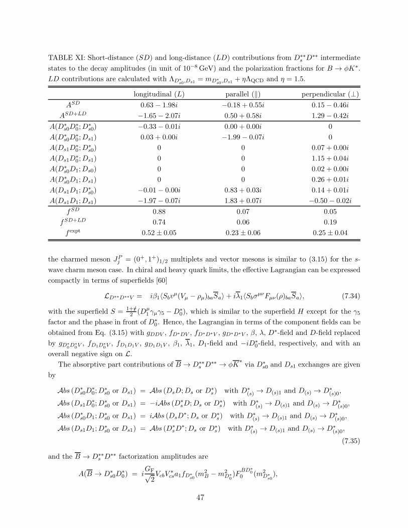
TABLE XI: Short-distance (SD) and long-distance (LD) contributions from D∗∗s D

∗∗ intermediate

states to the decay amplitudes (in unit of 10−8 GeV) and the polarization fractions for B → φK∗.

LD contributions are calculated with ΛD∗s0,Ds1 = mD∗

s0,Ds1 + ηΛQCD and η = 1.5.

longitudinal (L) parallel (‖) perpendicular (⊥)

ASD 0.63 − 1.98i −0.18 + 0.55i 0.15 − 0.46i

ASD+LD −1.65− 2.07i 0.50 + 0.58i 1.29 − 0.42i

A(D∗s0D

∗0 ;D

∗s0) −0.33− 0.01i 0.00 + 0.00i 0

A(D∗s0D

∗0 ;Ds1) 0.03 + 0.00i −1.99 − 0.07i 0

A(Ds1D∗0 ;D

∗s0) 0 0 0.07 + 0.00i

A(Ds1D∗0 ;Ds1) 0 0 1.15 + 0.04i

A(D∗s0D1;Ds0) 0 0 0.02 + 0.00i

A(D∗s0D1;Ds1) 0 0 0.26 + 0.01i

A(Ds1D1;D∗s0) −0.01− 0.00i 0.83 + 0.03i 0.14 + 0.01i

A(Ds1D1;Ds1) −1.97− 0.07i 1.83 + 0.07i −0.50 − 0.02i

fSD 0.88 0.07 0.05

fSD+LD 0.74 0.06 0.19

f expt 0.52 ± 0.05 0.23 ± 0.06 0.25 ± 0.04

the charmed meson JPj = (0+, 1+)1/2 multiplets and vector mesons is similar to (3.15) for the s-

wave charm meson case. In chiral and heavy quark limits, the effective Lagrangian can be expressed

compactly in terms of superfields [60]

LD∗∗D∗∗V = iβ1〈Sbvµ(Vµ − ρµ)baSa〉+ iλ1〈SbσµνFµν(ρ)baSa〉, (7.34)

with the superfield S = 1+v/2 (Dµ

1 γµγ5 −D∗0), which is similar to the superfield H except for the γ5

factor and the phase in front of D∗0 . Hence, the Lagrangian in terms of the component fields can be

obtained from Eq. (3.15) with gDDV , fD∗DV , fD∗D∗V , gD∗D∗V , β, λ, D∗-field and D-field replaced

by gD∗0D

∗0V

, fD1D∗0V

, fD1D1V , gD1D1V , β1, λ1, D1-field and −iD∗0-field, respectively, and with an

overall negative sign on L.The absorptive part contributions of B → D∗∗

s D∗∗ → φK

∗via D∗

s0 and Ds1 exchanges are given

by

Abs (D∗s0D

∗0;D

∗s0 or Ds1) = Abs (DsD;Ds or D

∗s) with D∗

(s) → D(s)1 and D(s) → D∗(s)0,

Abs (Ds1D∗0;D

∗s0 or Ds1) = −iAbs (D∗

sD;Ds or D∗s) with D∗

(s) → D(s)1 and D(s) → D∗(s)0,

Abs (D∗s0D1;D

∗s0 or Ds1) = iAbs (DsD

∗;Ds or D∗s) with D∗

(s) → D(s)1 and D(s) → D∗(s)0,

Abs (Ds1D1;D∗s0 or Ds1) = Abs (D∗

sD∗;Ds or D

∗s) with D∗

(s) → D(s)1 and D(s) → D∗(s)0,

(7.35)

and the B → D∗∗s D

∗∗ factorization amplitudes are

A(B → D∗s0D

∗0) = i

GF√2VcbV

∗csa1fD∗

s0(m2

B −m2D∗

0)F

BD∗0

0 (m2D∗

s0),

47

A(B → Ds1D∗0) = −iGF√

2VcbV

∗csa1fDs1mDs1F

BD∗0

1 (m2Ds1

)(2ε∗Ds1· pB),

A(B → D∗s0D1) = −iGF√

2VcbV

∗csa1fD∗

s0mD1V

BD10 (m2

D∗s0)(2ε∗D1

· pB),

A(B → D∗sD

∗) = iGF√2VcbV

∗csa1fDs1mDs1(mB −mD1)ε

∗µDs1

ε∗νD1

[

V BD11 (m2

Ds1)gµν

−2V BD1

2 (m2Ds1

)

(mB −mD∗)2pBµpBν − i

2ABD1(m2Ds1

)

(mB −mD∗)2ǫµναβp

αBp

βD1

]

. (7.36)

with decay constants and form factors given in [63]. Note that the −i and i factors appearing in

(7.35) originate from the phases differences ofD∗(s)0 andD(s) in the superfields S andH, respectively.

From these equations, it is now evident that the contributions from B → Ds1D∗0 → φK

∗and

B → D∗s0D1 → φK

∗rescatterings add up instead of cancellation as noticed before. To estimate

the numerical significance of these contributions, we shall use β1 = 1(≃ β), λ1 = 1GeV−1(≃ λ)

and ΛD∗s0,Ds1 = mD∗

s0,Ds1 + ηΛQCD with η = 1.5 and the monopole form for the form factors

F (t,mD∗s) and F (t,mDs1). Numerical results are shown in Table XI. The branching ratio is

BSD+LD(B → φK∗) = 8.4 × 10−6. It is interesting to notice that most of the FSI contributions

from the intermediate D∗∗s D

∗∗ states add up in A⊥ giving f⊥ ≃ 0.2, which is close to data. Note

that we only consider the contribution from Ds1/2D1/2 intermediate states. A more detailed study

including other multiplets such as D3/2 along this line is worth pursuing.

F. Comparison with other works

Although the analysis of the φK∗ polarization anomaly by Colangelo, De Fazio and Pham

(CDP) [78] is very similar to ours, their results are quite different form ours in some respects (see

also [85] for a different analysis based on the Regge theory). First, in our case, the interference

between short-distance and long-distance contributions is mild because the absorptive long-distance

contribution is essentially “orthogonal” to the short-distance one (see Table IX). By fixing Λ = 2.3

GeV, to be compared with our choice of ΛDs,D∗s= mDs,D∗

s+ ηΛQCD with η = 0.8, CDP introduced

a parameter r so that A = ASD + rALD with r = 0 corresponding to the absence of rescattering.

It appears from Fig. 3 of [78] that there is a drastic SD and LD interference behavior in the CDP

calculation, namely, the resulting branching ratio is not symmetric with respect to the reflection of r:

r → −r. It is not clear to us why the absorptive LD contribution obtained by CDP is not orthogonal

to the SD one at all. Second, instead of employing a small r factor of order 0.08 to reduce the

FSI contribution, we use the form factors with different momentum dependence for the exchanged

particles Ds and D∗s . As a result, fL ≈ 1/2 can be accommodated in our work with a reasonable

cutoff. Third, we have shown large cancellations occurring in the processes B → D∗sD → φK

∗

and B → DsD∗ → φK

∗and this can be understood as a consequence of CP and SU(3) [CPS]

symmetry. We are not able to check the aforementioned cancellation in the CDP work as no details

are offered to the individual LD amplitudes. Anyway, f⊥ is very small (of order 3%) in our case,

while CDP obtained f⊥ ≈ 0.15. Fourth, CDP adapt a different phase convention for pseudoscalar

mesons. Considerable efforts have been made in keeping the consistency of phase conventions and

48

reminders on phase subtleties (see, for example, footnote 2 on p.11) are given in this work. On

the other hand, as far as the analytic expressions are concerned we do not find any inconsistency

in the phase convention chosen in the CDP work. Fifth, we apply the U(3) symmetry for the φ

meson, while CDP seem to consider only the ω8 component of it. Since in both approaches φ always

couples to a D(∗)s D

(∗)s pair (see Fig. 9 in this work and Fig. 2 in [78]), only the ss component of φ is

relevant. Hence, the FSI amplitudes in CDP should be identical to ours up to an overall factor of

the Clebsch-Gordan coefficient, −2/√6. We do not expect any qualitative difference arising from

the different treatments of the φ wave function. In particular, the cancellation argument presented

in Sec. VII.C should be also applicable to their case.

Working in the context of QCD factorization, Kagan [26] has recently argued that the lower value

of the longitudinal polarization fraction can be accommodated in the Standard Model provided that

the penguin-induced annihilation contributions are taken into account. In general, the annihilation

amplitudes induced by the (V −A)(V − A) operators are subject to helicity suppression. Indeed,

they are formally power suppressed by order (ΛQCD/mb)2 [17]. However, the (S − P )(S + P )

penguin operator induced annihilation is no longer subject to helicity suppression and could be

substantially enhanced. In QCD factorization, the penguin-induced annihilation amplitude contains

some infrared divergent integral, say XA, arising from the logarithmic endpoint divergence, and

the logarithmic divergence squared X2A. Modelling the logarithmic divergence by [17]

XA = (1 + ρAeiφA) ln

mB

Λh, (7.37)

with Λh being a hadron scale of order 500 MeV and ρA ≤ 1, Kagan has shown that the φK∗

polarization measurements can be accommodated by fitting to the annihilation parameter ρA (see

Fig. 4 of [26]). Note that the penguin-induced annihilation terms being formally of order 1/m2b do

respect the scaling law stated in Eq. (7.1), but they can be O(1) numerically.

Assuming Kagan’s reasoning [27] is correct, it means that although QCD factorization does not

predict a lower value of the φK∗ longitudinal polarization, one may be able to find a value for ρA

within an acceptable range to be able to accommodate the data.

It is worth mentioning also that the annihilation amplitudes in V V modes are calculable in

the so-called perturbative QCD approach for hadronic B decays where the end-point divergence is

regulated by the parton’s transverse momentum. In particular, the B → φK∗ decay is studied in

[86], giving fL : f‖ : f⊥ = 0.75 : 0.13 : 0.11 and B(B− → φK∗−) = 16.0 × 10−6. Although fL is

reduced after the inclusion of nonfactorizable and annihilation contributions, f‖,⊥ are only of order

10%. The annihilation contribution indeed helps but it is not sufficient.

A common feature of the final-state rescattering or a large penguin-induced annihilation contri-

bution as a mechanism for explaining the observed φK∗ anomaly is that the same mechanism will

also lead to a large transverse polarization in the ρK∗ modes, which is borne out by experiment

in the decay B− → ρ−K∗0

but not in B− → ρ0K∗− (see Table VII). This has to be clarified

experimentally.

An alternative suggestion for the solution of the φK∗ anomaly was advocated in [87] that a

energetic transverse gluon from the b → sg chromodipole operator keeps most of its quantum

numbers except color when it somehow penetrates through the B meson surface and descends

49

to a transversely polarized φ meson. Sizable transverse components of the B → φK∗ decay can

be accommodated by having f‖ > f⊥ (see also Table VIII). Since the gluon is a flavor singlet,

this mechanism can distinguish φ from ρ, hence it affects B → φK∗, ωK

∗but not B → K

∗ρ. The

B → ωK∗is predicted to be of order 4×10−6 with large transverse components. On the other hand,

a recent estimation based on PQCD [88] seems to indicate the above-mentioned contribution is too

small to explain the φK∗anomaly. Moreover, the predicted absence of the transverse polarization

in B → ρK∗ is not consistent with experiment at least for ρ−K∗0

and ρ+K∗− modes.

VIII. DISCUSSION AND CONCLUSION

In this work we have studied the effects of final-state interactions on the hadronic B decay rates

and their impact on direct CP violation. Such effects are modelled as soft final-state rescattering

of some leading intermediate two-body channels and can be classified according to the topological

quark diagrams. It amounts to considering the one-particle-exchange processes at the hadron level

for long-distance rescattering effects. Our main results are as follows:

1. The color-suppressed neutral modes such as B0 → D0π0, π0π0, ρ0π0,K0π0 can be substan-

tially enhanced by long-distance rescattering effects, whereas the color-allowed modes are

not significantly affected by FSIs.

2. All measured color-suppressed charmful decays of B0into D(∗)0π0,D0η,D0ω and D0ρ0 are

significantly larger than theoretical expectations based on naive factorization. The rescat-

tering from B → {Dπ,D∗ρ} → Dπ contributes to the color-suppressed W -emission and

W -exchange topologies and accounts for the observed enhancement of the D0π0 mode with-

out arbitrarily assigning the ratio of a2/a1 a large magnitude and strong phase as done in

many previous works.

3. The branching ratios of all penguin-dominated B → πK decays are enhanced via final-state

rescattering effects by (30-40)%. CP asymmetry in the K−π+ mode is predicted by the

short-distance approach to be ∼ 4%. It is modified by final-state rescattering to the level of

14% with a sign flip, in good agreement with the world average of −0.11 ± 0.02. Given the

establishment of direct CP violation in B0 → K−π+, a model-independent relation assuming

SU(3) implies that the π+π− mode has direct CP asymmetry of order 40% with a positive

sign. An isospin sum-rule relation involving the branching ratios and CP asymmetries of the

four B → Kπ modes indicates the presence of electroweak contributions and/or some New

Physics. Better measurements are needed to put this on a firmer footing.

4. If only the absorptive part of final-state rescattering is considered, it cannot explain the

observed enhancement of the π0π0 rate, whereas the predicted π+π− will be too large by

a factor of 2 compared to experiment. The dispersive part of rescattering from DD → ππ

and ππ → ππ via meson annihilation (i.e. the so-called vertical W -loop diagram V) which

interferes destructively with the short-distance amplitude of B0 → π+π− can reduce π+π−

and enhance π0π0 substantially.

50

5. For tree-dominated B → ππ decays, it is known that the predicted direct CP asymmetry

in the π+π− mode by the short-distance approach is small with a negative sign. We have

shown that its sign is flipped by final-state rescattering and its magnitude is substantially

enhanced. Direct CP violation in B → π0π0 is predicted to have a sign opposite to that of

π+π−, in contrast to the predictions based on perturbative QCD (PQCD). Hence, even a

sign measurement of direct CP asymmetry in π0π0 can be used to discriminate between the

FSI and PQCD approaches for CP violation.

6. CP partial rate asymmetry in B± → π±π0 is very small in the SM and remains so even

after the inclusion of FSIs, with a magnitude less than 1 percent. Since CP asymmetry is

caused by the electroweak penguin but not the QCD penguin (up to isospin violation), this

is a good mode for searching New Physics.

7. For tree-dominated B → ρπ decays, we showed that (i) the color-suppressed ρ0π0 mode is

slightly enhanced by rescattering effects to the order of 1.3×10−6, which is consistent with the

weighted average of the experimental values. However, the discrepancy between BaBar and

Belle for this mode should be clarified soon. It should be stressed that direct CP violation in

this mode is significantly enhanced by FSI from around 1% to 60%. (ii) Direct CP violation

in the ρ+π− mode is greatly enhanced by FSI from the naive expectation of ∼ −0.01 from

the short-distance approach to the level of −0.42, in agreement with BaBar and Belle.

8. As for the intriguing B → φK∗ polarization anomaly, the longitudinal polarization fraction

can be significantly reduced by the rescattering contribution from the intermediate DDs

states. However, no sizable perpendicular polarization is found owing mainly to the large

cancellations among various contributions from intermediate DsD∗ and D∗

sD states. Conse-

quently, our result for the perpendicular polarization fraction is different from a recent similar

analysis in [78]. Final-state rescattering effects from this particular set of states seem not be

able to fully account for the polarization anomaly observed in B → φK∗ and FSI from other

intermediate states and/or some other mechanism e.g. the penguin-induced annihilation [27],

may have to be invoked. Given the fact that both Belle and BaBar observe large phases in

various polarization amplitudes (see Table VII), FSI may still provide a plausible explana-

tion. In any case, our conclusion is that the small value of the longitudinal polarization in

V V modes cannot be regarded as a clean signal for New Physics.

Needless to say, the calculation of final-state rescattering effects in hadronic B decays is rather

complicated and very much involved and hence it suffers from several possible theoretical uncer-

tainties. Though most of them have been discussed before, it is useful to make a summary here:

(i) The strong form factor F (t) for the off-shell effects of the exchanged particle. It is param-

eterized as in Eq. (3.22) by introducing a cutoff scale Λ. Moreover, we write Λ = mexc + ηΛQCD

[cf. Eq. (3.40)], where the parameter η is expected to be of order unity and can be determined

from the measured rates. For a given exchanged particle, the cutoff varies from process to process.

For example, ηD = 2.1, 0.69, 1.6 for B → Dπ,Kπ, ρπ decays, respectively. To see the sensitivity

on the cutoff, we have allowed 15% error in the QCD scale ΛQCD. Another important uncertainty

51

arises from the momentum dependence of the form factor F (t). Normally it is assumed to be of the

monopole form. However, the analysis of the φK∗ decays prefers to a dipole behavior for the form

factor F (t,mD∗s) appearing in the VexcV P or VexcV V vertex with the exchanged vector particle

Vexc and a monopole dependence for other form factors. A more rigorous study of the momentum

dependence of the strong form factor is needed. It turns out that CP asymmetries and the decay

rates especially for the color-suppressed modes are in general sensitive to the cutoff scale. This

constitutes the major theoretical uncertainties for long-distance rescattering effects.

(ii) Form factors and decay constants. Model predictions for the form factors can vary as much

as 30% which in turn imply large uncertainties in the branching ratios. In particular, the B → V V

decays are fairly sensitive to the difference between the form factors A1 and A2. For form factor

transitions in this work we rely on the covariant light-front model which is favored by the current

data.

(iii) Strong couplings of heavy mesons and their SU(3) breaking. We have applied chiral and

heavy quark symmetries to relate various strong couplings of heavy mesons with the light pseu-

doscalar or vector mesons. It is not clear how important are the chiral and 1/mQ corrections. For

SU(3) breaking effects, we have assumed that they are taken into account in the relations given in

Eqs. (4.12) and (7.9).

(iv) The real part of the long-distance contribution which can be obtained from the disper-

sion relation (3.39). Unlike the absorptive part, the dispersive contribution suffers from the large

uncertainties due to some possible subtractions and the complication from integrations. For this

reason, we have ignored it so far. However, in order to resolve the discrepancy between theory

and experiment for B0 → π+π− and B0 → π0π0, we have argued that it is the dispersive part of

long-distance rescattering of DD → ππ and ππ → ππ via meson annihilation that accounts for the

suppression of the π+π− mode and the enhancement of π0π0.

(v) CKM matrix elements and γ. Direct CP asymmetry is proportional to sin γ. All numbers

in the present work are generated by using γ = 60◦.

(vi) Intermediate multi-body contributions which have not been considered thus far and may

have cancellations with the contributions from two-body channels.

Finally, it is worth remarking that the final-state rescattering effects from intermediate charmed

mesons as elaborated in the present work has some similarity to the long-distance “charming pen-

guin” effects advocated in the literature [32, 33, 34]. The relevance of this long-distance effect has

been conjectured to be justified in the so-called soft collinear effective theory [89]. Indeed, we have

pointed out that some of the charmed meson loop diagrams in the decays e.g. B → ππ, πK, φK∗

will manifest as the long-distance cc penguins. However, we have also considered FSIs free of

charming penguins. For example, long-distance rescattering effects in B → Dπ and in B− → π−π0

(also ρ−ρ0) decays have nothing to do with the charming penguin effects. In other words, our

systematic approach for FSIs goes beyond the long-distance charming penguin mechanism.

52

Acknowledgments

We are grateful to Andrei V. Gritsan for helpful discussions on B to V V data. This research was

supported in part by the National Science Council of R.O.C. under Grant Nos. NSC93-2112-M-

001-043, NSC93-2112-M-001-053 and by the U.S. DOE contract No. DE-AC02-98CH10886(BNL).

53

APPENDIX A: USEFUL FORMULA

Under the integration, the covariant integrals∫

d3~p1(2π)32E1

d3~p2(2π)32E2

(2π)4δ4(pB − p1 − p2)f(t)× {p1µ, p1µp1ν , p1µp1νp1α} (A1)

can only be expressed by external momenta p3, p4 with suitable Lorentz and permutation structures.

Hence we can express these p1µ, p1µp1ν , p1µp1νp1α in terms for P = p3 + p4 and q = p3 − p4 as in

Eq. (7.12) within the integration. By contracting the left-hand side of Eq. (7.12) with Pµ, qµ and

gµν , we are able to solve for these A(i)j and obtain

(

A(1)1

A(1)2

)

=

(

P 2 P · qP · q q2

)−1

·(

P · p1q · p1

)

,

A(2)1

A(2)2

A(2)3

A(2)4

=

4 P 2 2P · q q2

P 2 (P 2)2 2P 2P · q (P · q)22P · q 2P 2P · q 2P 2q2 + (P · q)2 2P · qq2q2 (P · q)2 2P · qq2 q2

−1

·

p21(P · p1)2

2P · p1p1 · q(q · p1)2

,

A(3)1

A(3)2

A(3)3

A(3)4

A(3)5

A(3)6

=

18P 2 18P · q 3(P 2)2 9P 2P · q 3q2P 2 + 6(P · q)2 3q2P · q18q2 3P 2P · q 3P 2q2 + 6(P · q)2 9q2P · q 3(q2)2

(P 2)3 3(P 2)2P · q 3(P · q)2P 2 (P · q)3

3(P 2)2q2 + 6P 2(P · q)2 3(P · q)3 + 6P 2q2P · q 3(P · q)2q2

3(q2)2P 2 + 6q2(P · q)2 3(q2)2P · q(q2)3

−1

·

3m21P · p1

3m21q · p1

(P · p1)33(P · p1)2p1 · q3(q · p1)2p1 · P

(q · p1)3

, (A2)

where the lower left part of the symmetric inverse matrix for the A(3)j case is not shown explicitly.

Note that the t dependence of A(i)j is in the column matrices in the right-hand side of the above

equations and t always appears in the numerators of A(i)j in a polynomial form.

APPENDIX B: THEORETICAL INPUT PARAMETERS

In this Appendix we summarize the input parameters used in the present paper. For decay

constants we use

fπ = 132MeV, fK = 160MeV, fD = 200MeV, fD∗ = 230MeV, fa1 = −205MeV. (B1)

Note that a preliminary CLEO measurement of the semileptonic decay D+ → µ+ν yields fD+ =

(202 ± 41 ± 17) MeV [90]. For form factors we follow the covariant light-front approach [63]. For

54

purpose of comparison, we list some of the form factors at q2 = 0 used in the main text:

FBπ0 (0) = 0.25, FBK0 (0) = 0.35, ABρ0 (0) = 0.28, ABK∗

0 (0) = 0.31 (B2)

to be compared with

FBπ0 (0) = 0.28 ± 0.05, FBK0 (0) = 0.34 ± 0.05, ABρ0 (0) = 0.37 ± 0.06, ABK∗

0 (0) = 0.45 ± 0.07

(B3)

employed in [18] and

FBπ0 (0) = 0.33, FBK0 (0) = 0.38, ABρ0 (0) = 0.28, ABK∗

0 (0) = 0.32 (B4)

used by Bauer, Stech and Wirbel [91]. The most recent light-cone sum rule analysis yields [92]

FBπ0 (0) = 0.258 ± 0.031, FBK0 (0) = 0.331 + 0.041 + 0.025δa1 (B5)

with δa1 being defined in [92]. The B− → π−π0 data favors a smaller FBπ(0) of order 0.25, while

B → ρπ measurement prefers to small form factors for B → ρ transition.

For the quark mixing matrix elements, we use A = 0.801 and λ = 0.2265 [71] in the Wolfenstein

parametrization of the quark mixing angles [93]. The other two Wolfenstein parameters ρ and η

obey the relations η = R sin γ and ρ = R cos γ, where R = |VudV ∗ub/(VcdV

∗cb)|, ρ = (1 − λ2/2)ρ and

η = (1 − λ2/2)η. We take γ = 60◦ and R = 0.39 in this work for calculations. For current quark

masses, we usemb(mb) = 4.4 GeV,mc(mb) = 1.3 GeV,ms(2.1GeV) = 90 MeV andmq/ms = 0.044.

The physical strong coupling constants are

gρππ = 6.05 ± 0.02, gK∗Kπ = 4.6, gD∗Dπ = 17.9 ± 0.3 ± 1.9,

gV = 5.8, β = 0.9, λ = 0.56GeV−1, (B6)

where gV , β and λ (not to be confused with the parameter λ appearing in the parametrization of

quark mixing angles) are the parameters in the effective chiral Lagrangian describing the interac-

tions of heavy mesons with low momentum light vector mesons.

55

[1] Belle Collaboration, K. Abe et al., Phys. Rev. Lett. 88, 031802 (2002).

[2] BaBar Collaboration, B. Aubert et al., hep-ex/0207066.

[3] B. Melic, hep-ph/0404003.

[4] Z.G. Wang, L. Li, and T. Huang, hep-ph/0311296.

[5] P. Colangelo, F. De Fazio, and T. N. Pham, Phys. Lett. B 542, 71 (2002); Phys. Rev. D 69,

054023.

[6] Belle Collaboration, K. Abe et al., hep-ex/0409004.

[7] CLEO Collaboration, T.E. Coan et al., Phys. Rev. Lett. 88, 062001 (2002).

[8] BaBar Collaboration, B. Aubert et al., Phys. Rev. D 69, 032004 (2004).

[9] H.Y. Cheng, Phys. Rev. D 65, 094012 (2002).

[10] C.W. Chiang, M. Gronau, J.L. Rosner, and D. Suprun, Phys. Rev. D 70, 034020 (2004).

[11] BaBar Collaboration, B. Aubert et al., Phys. Rev. Lett. 91, 241801 (2003).

[12] Belle Collaboration, S.H. Lee et al., Phys. Rev. Lett. 91, 261801 (2003).

[13] C.D. Lu and M.Z. Yang, Eur. Phys. J. C 23 275 (2002).

[14] BaBar Collaboration, B. Aubert et al., hep-ex/0407057.

[15] Belle Collaboration, Y. Chao et al., hep-ex/0407025.

[16] Belle Collaboration, Y. Chao et al., hep-ex/0408100.

[17] M. Beneke, G. Buchalla, M. Neubert, and C.T. Sachrajda, Phys. Rev. Lett. 83, 1914 (1999);

Nucl. Phys. B 591, 313 (2000); ibid. B606, 245 (2001).

[18] M. Beneke and M. Neubert, Nucl. Phys. B 675, 333 (2003).

[19] Belle Collaboration, K. Abe et al., Phys. Rev. Lett. 93, 021601 (2004).

[20] BaBar Collaboration, B. Aubert et al., hep-ex/0408089.

[21] Belle Collaboration, Y. Sakai , plenery talk at 32nd International Conference on High Energy

Physics, August, 2004, Beijing, China; BaBar Collaboration, M. Giorgi , plenery talk at 32nd

International Conference on High Energy Physics, August, 2004, Beijing, China.

[22] Belle Collaboration, P. Krokovny et al., Phys. Rev. Lett. 89, 231804 (2002).

[23] BaBar Collaboration, B. Aubert et al., Phys. Rev. Lett. 90, 181803 (2003).

[24] BaBar Collaboration, B. Aubert et al., Phys. Rev. Lett. 91, 171802 (2003); hep-ex/0303020.

[25] Belle Collaboration, K.F. Chen et al., Phys. Rev. Lett. 91, 201801 (2003).

[26] A.L. Kagan, Phys. Lett. B 601, 151 (2004).

[27] A.L. Kagan, hep-ph/0407076.

[28] D. Atwood and A. Soni, Phys. Rev. D 58, 036005 (1998).

[29] M. Bander, D. Silverman, and A. Soni, Phys. Rev. Lett. 43, 242 (1979).

[30] Y. Lu, B.S. Zou, and M.P. Locher, Z. Phys. A 345, 207 (1993); M.P. Locher, Y. Lu, and B.S.

Zou, ibid 347, 281 (1994); X.Q. Li and B.S. Zou, Phys. Lett. B 399, 297 (1997); Y.S. Dai,

D.S. Du, X.Q. Li, Z.T. Wei, and B.S. Zou, Phys. Rev. D 60, 014014 (1999).

[31] M. Ablikim, D.S. Du, and M.Z. Yang, Phys. Lett. B 536, 34 (2002); J.W. Li, M.Z. Yang, and

D.S. Du, hep-ph/0206154.

56

[32] M. Ciuchini et al., Nucl. Phys. B 501, 271 (1997); ibid. 512, 3 (1998); hep-ph/0407073.

[33] P. Colangelo, G. Nardulli, N. Paver, and Riazuddin, Z. Phys. C 45, 575 (1990); G. Isola, M.

Ladisa, G. Nardulli, T.N. Pham, and P. Santorelli, Phys. Rev. D 64, 014029 (2001); ibid. 65,

094005 (2002).

[34] G. Isola, M. Ladisa, G. Nardulli, and P. Santorelli, Phys. Rev. D 68, 114001 (2003).

[35] S. Barshay, L.M. Sehgal, and J. van Leusen, Phys. Lett. B 591, 97 (2004).

[36] S. Barshay, G. Kreyerhoff, and L.M. Sehgal, Phys. Lett. B 595, 318 (2004).

[37] J.F. Donoghue, E. Golowich, A.A. Petrov, and J.M. Soares, Phys. Rev. Lett. 77, 2178 (1996);

H. Lipkin, Phys. Lett. B 415, 186 (1997); D. Delepine, J.M. Gerard, J. Pestieau, and J.

Weyers, Phys. Lett. B 429, 106 (1998); A.F. Falk, A.L. Kagan, Y. Nir, and A.A. Petrov,

Phys. Rev. D 57, 4290 (1998); M. Suzuki and L. Wolfenstein, ibid. 60, 074019 (1999); A.N.

Kamal, ibid. 60, 094018 (1999); D.S. Du, X.Q. Li, Z.T. Wei, and B.S. Zou, Eur. Phys. J. A

4, 91 (1999); N.G. Deshpande, X.G. He, W.S. Hou, and S. Pavasa, Phys. Rev. Lett. 82, 2240

(1999); W.S. Hou and K.C. Yang, ibid. 84, 4806 (2000).

[38] C.K. Chua, W.S. Hou, and K.C. Yang, Mod. Phys. Lett. A 18, 1763 (2003).

[39] M. Beneke, G. Buchalla, M. Neubert, and C.T. Sachrajda, Nucl. Phys. B 606, 245 (2001).

[40] C. Smith, Eur. Phys. J. C 33, 523 (2004).

[41] G. t’ Hooft, Nucl. Phys. B 72, 461 (1974); A.J. Buras, J.-M. Gerard, amd R. Ruckl, ibid.

268, 16 (1986).

[42] L.L. Chau and H.Y. Cheng, Phys. Rev. D 36, 137 (1987); Phys. Lett. B 222, 285 (1989).

[43] L.L. Chau, Phys. Rep. 95, 1 (1983).

[44] L.L. Chau and H.Y. Cheng, Phys. Rev. Lett. 56, 1655 (1986).

[45] J.F. Donoghue, Phys. Rev. D 33, 1516 (1986).

[46] El hassan El aaoud and A.N. Kamal, Int. J. Mod. Phys. A 15, 4163 (2000).

[47] P. Zenczykowski, Acta Phys. Polon. B 28, 1605 (1997) [hep-ph/9601265].

[48] S. Weinberg, The Quantum Theory of Fields, Volume I (Cambridge, 1995), Sec. 3.8.

[49] H.Y. Cheng, Eur. Phys. J. C 26, 551 (2003).

[50] Particle Data Group, S. Eidelman et al., Phys. Lett. B 592, 1 (2004).

[51] C.W. Chiang and J.L. Rosner, Phys. Rev. D 67, 074013 (2003).

[52] J.L. Rosner, Phys. Rev. D 60, 114026 (1999).

[53] H.Y. Cheng and K.C. Yang, Phys. Rev. D 59, 092004 (1999).

[54] Z.Z. Xing, hep-ph/0107257.

[55] M. Neubert and A.A. Petrov, Phys. Lett. B 519, 50 (2001).

[56] J.P. Lee, hep-ph/0109101.

[57] C.K. Chua, W.S. Hou, and K.C. Yang, Phys. Rev. D 65, 096007 (2002).

[58] Y.Y. Keum, T. Kurimoto, H.n. Li, C.D. Lu, and A.I. Sanda, Phys. Rev. D 69, 094018 (2004).

[59] S. Mantry, D. Pirjol, and I.W. Stewart, Phys. Rev. D 68, 114009 (2003).

[60] R. Casalbuoni, A. Deandrea, N. Di Bartolomeo, R. Gatto, F. Feruglio, and G. Nardulli, Phys.

Rep. 281, 145 (1997).

[61] T. M. Yan, H. Y. Cheng, C. Y. Cheung, G. L. Lin, Y. C. Lin, and H. L. Yu, Phys. Rev. D 46,

1148 (1992); 55, 5851(E) (1997); M. B. Wise, Phys. Rev. D 45, R2188 (1992); G. Burdman

57

and J. Donoghue, Phys. Lett. B 280, 287 (1992).

[62] O. Gortchakov, M.P. Locher, V.E. Markushin, and S. von Rotz, Z. Phys. A 353, 447 (1996).

[63] H. Y. Cheng, C. K. Chua, and C. W. Hwang, Phys. Rev. D 69, 074025 (2004).

[64] CLEO Collaboration, S. Ahmed et al., Phys. Rev. Lett. 87, 251801 (2001).

[65] Heavy Flavor Averaging Group, http://www.slac.stanford.edu/xorg/hfag.

[66] A. Ali and C. Greub, Phys. Rev. D 57, 2996 (1998); A. Ali, G. Kramer, and C.D. Lu, ibid.

58, 094009 (1998).

[67] Y.H. Chen, H.Y. Cheng, B. Tseng, and K.C. Yang, Phys. Rev. D 60, 094014 (1999).

[68] Z. Ligeti, hep-ph/0408267.

[69] Y.Y. Keum, H.n. Li, and A.I. Sanda, Phys. Rev. D 63, 054008 (2001); Y.Y. Keum, talk

presented at WHEPP-8 Workshop, Mumbai, India, January 2004.

[70] A.J. Buras, R. Fleischer, S. Recksiegel, and F. Schwab, Nucl. Phys. B 697, 133 (2004).

[71] CKMfitter Group, J. Charles et al., hep-ph/0406184.

[72] M. Pivk and F.R. Le Diberder, hep-ph/0406263.

[73] N.G. Deshpande and X.G. He, Phys. Rev. Lett. 75, 1703 (1995).

[74] BaBar Collaboration, B. Aubert et al., Phys. Rev. D 69, 031102 (2004); hep-ex/0408017;

hep-ex/0408063; hep-ex/0408093; hep-ex/0411054; A. Gritsan, hep-ex/0409059.

[75] Belle Collaboration, J. Zhang et al., ibid. 91, 221801 (2003); K. Abe et al., hep-ex/0408141.

[76] A.S. Dighe, M. Gronau, and J.L. Rosner, Phys. Rev. Lett. 79, 4333 (1997).

[77] H.Y. Cheng and K.C. Yang, Phys. Lett. B 511, 40 (2001).

[78] P. Colangelo, F. De Fazio and T. N. Pham, Phys. Lett. B 597, 291 (2004).

[79] P. Ball and V.M. Braun, Phys. Rev. D 58, 094016 (1998); P. Ball, J. High Energy Phys. 09,

005 (1998).

[80] P. Ball, hep-ph/0306251.

[81] BaBar Collaboration, B. Aubert et al., hep-ex/0408017.

[82] C.W. Bernard, T. Draper, A. Soni, H.D. Politzer, and M.B. Wise, Phys. Rev. D 32, 2343

(1985); C.W. Bernard, T. Draper, G. Hockney, and A. Soni, Nucl. Phys. Proc. Suppl. 4, 483

(1988); C. Dawson, G. Martinelli, G.C. Rossi, C.T. Sachrajda, S.R. Sharpe, M. Talevi, and

M. Testa, Nucl. Phys. B 514, 313 (1998).

[83] See also X.G. He, X.Q. Li, and J.P. Ma, hep-ph/0407083.

[84] A. Seiden, H. F. W. Sadrozinski, and H. E. Haber, Phys. Rev. D 38, 824 (1988); L. Kopke

and N. Wermes, Phys. Rep. 174, 67 (1989).

[85] M. Ladisa, V. Laporta, G. Nardulli, and P. Santorelli, hep-ph/0409286.

[86] C.H. Chen, Y.Y. Keum, and H-n. Li, Phys. Rev. D 66, 054013 (2002).

[87] W.S. Hou and M. Nagashima, hep-ph/0408007.

[88] H-n. Li, hep-ph/0408232.

[89] C.W. Bauer, D. Pirjol, I.Z. Rothstein, and I.W. Stewart, hep-ph/0401188.

[90] CLEO Collaboration, G. Bonvicini et al., hep-ex/0411050; D. Besson et al., hep-ex/0408071.

[91] M. Wirbel, B. Stech, and M. Bauer, Z. Phys. C 29, 637 (1985); M. Bauer, B. Stech, and M.

Wirbel, ibid. 34, 103 (1987).

[92] P. Ball and R. Zwicky, hep-ph/0406232.

58

[93] L. Wolfenstein, Phys. Rev. Lett. 51, 1945 (1983).

59