Board of Governors of the Federal Reserve System

International Finance Discussion Papers

Number 559

July 1996

BROAD MONEY DEMAND AND FINANCIAL LIBERALIZATION

IN GREECE

Neil R. Ericsson and Sunil Sharma

NOTE: International Finance Discussion Papers are preliminary materials circulated

to stimulate discussion and critical comment. References in publications to Interna-

tional Finance Discussion Papers (other than an acknowledgment that the writer has

had access to unpublished material) should be cleared with the author or authors.

Abstract

This paper develops a constant, data-coherent, error correction model

for broad money demand (M3) in Greece. This model contributes to a

better understanding of the e®ects of monetary policy in Greece, and of

the portfolio consequences of ¯nancial innovation in general. The broad

monetary aggregate M3 was targeted until recently, and current monetary

policy still uses such aggregates as guidelines, yet analysis of this aggregate

has been dormant for over a decade.

In spite of large °uctuations in the in°ation rate, introduction of new

¯nancial instruments, and liberalization of the ¯nancial system, the esti-

mated model is remarkably stable. The dynamics of money demand are

important, with price and income elasticities being much smaller in the

short run than in the long run.

Keywords: broad money, cointegration, conditional models, dynamic speci-

¯cation, error correction, exogeneity, ¯nancial liberalization, ¯nancial in-

novation, general-to-speci¯c modeling, Greece, money demand, sequential

reduction, vector autoregression.

Broad Money Demand and Financial Liberalization in GreeceNeil R. Ericsson and Sunil Sharma¤

I. Introduction

Recent changes in the Greek financial system pose challenges for the conduct of monetarypolicy. The removal of most external capital controls and the abolition of restrictions onthe portfolios of deposit-taking institutions have substantially changed the environmentin which monetary policy operates. The interbank market has deepened, interest rates aremore flexible, and new indirect instruments of monetary control are being developed.

At the operational level, the monetary program prepared by the Bank of Greece atthe beginning of each year defines the monetary policy of the authorities. Until recently,its formulation focussed on the determination of the appropriate growth of broad money(M3) on the basis of projections for real output growth, inflation, interest rates, and thedesired external balance.1 From the projected path of M3, an estimate of the requiredincrease in net domestic credit was calculated. Given a separate assessment of the creditneeds of the private sector, the Bank could derive the credit expansion to the public sectorthat was consistent with these projections.

In light of fundamental changes to the financial system, the monetary authorities haverecently shifted to targeting the exchange rate.2 New financial products have complicatedthe choice of an appropriate monetary aggregate as a target. Besides requiring redefinitionof what constitutes “money,” these products have changed the characteristics of assetsthat were previously included in the monetary aggregates. Although easier to control,narrowly defined aggregates are less useful in policy, as their relationship with nominalincome appears subject to considerable variability. Broader aggregates appear more stablerelative to nominal income, but they are less amenable to control. In addition, Greece’sdifferential taxation of financial products has complicated the assessment of movements

¤ The authors are staff economists in the Division of International Finance, Federal Reserve Board,and the Research Department, International Monetary Fund, respectively. The views expressed in thispaper are solely the responsibility of the authors and should not be interpreted as reflecting those of theBoard of Governors of the Federal Reserve System, the International Monetary Fund, or other membersof their staffs. We wish to thank Sophocles Brissimis, Nicholas Paleocrassas, and George Simigiannisat the Bank of Greece for providing the data and offering insights into institutional aspects of the Greekfinancial system; and Richard Agenor, Caroline Atkinson, Adi Brender, Julia Campos, Dimitri Demekas,David Hendry, Tim Lane, and Jaime Marquez for useful discussions and comments. This paper is beingsimultaneously circulated as IMF Working Paper No.WP=96=62 by the International Monetary Fund andInternational Finance Discussion Paper No.559 by the Board of Governors of the Federal Reserve System.

1 The Bank of Greece also monitors a broader measure of liquidity, M4, which is defined as M3 plusgovernment paper with maturity of up to a year.

2 In 1995, the authorities’ monetary program announced a targeted rate of crawl of the Drachma/ECUexchange rate for the first time. Ranges for M3 and M4 growth were also specified to serve as guidelines.

– 2 –

in monetary aggregates.

The purpose of this paper is to model the empirical relationship between broadmoney, prices, real output, and interest rates, and to examine the constancy of thisrelationship, especially in light of recent changes in the financial system. In spite of itsimportance for forecasting and policy, constancy has proved elusive for estimated moneydemand functions of many countries; see Judd and Scadding (1982) for the United States.While nonconstant empirical equations do not preclude a stable underlying relation, theyleave unresolved the question of whether the observed predictive failure arises fromshifts in the underlying relation or whether it is simply a consequence of model mis-specification.

For Greek money demand, that question is moot. The estimated model is remarkablyconstant in spite of large fluctuations in the inflation rate, the introduction of new financialinstruments, and liberalization of the financial system. The long-run demand for realmoney depends upon real income with a unit elasticity, and on the own interest ratewith a semi-elasticity of approximately five. Assets outside money affect money demandthrough a spread between their rate of return and the rate of return on broad money. Thedynamics of money demand are important, with price and income elasticities being muchsmaller in the short run than in the long run.

This paper is organized as follows. Section II presents a brief historical perspectiveand discusses the economic theory of money demand and the data available. Section IIIanalyzes integration and cointegration properties of the data, testing for cointegration andweak exogeneity in a six-variable vector autoregression. The evidence on cointegrationties back directly to the economic theory of money demand. The empirical weak exo-geneity of prices, income, and interest rates provides the foundation for development ofa parsimonious, empirically constant, single-equation error correction model for moneydemand in Section IV. Section IV also examines the stability of the estimated moneydemand function in the face of financial liberalization over the period under considera-tion. Section V discusses some caveats and implications of the results, and Section VIconcludes. Appendix I describes the construction of the data, and Appendix II documentsthe design of the empirical error correction model.3

3 The data can be obtained by request from the authors at Internet addresses ericsson@frb.gov andssharma@imf.org. All numerical results were obtained using PcGive Professional Versions 8.10, 8.15,and 9.00 ; cf. Doornik and Hendry (1994). We are especially grateful to Jurgen Doornik and DavidHendry for providing us with an update to PcGive Professional (Version 8.15) and a pre-release version ofPcGive Professional for Windows (Version 9.00¯) .

– 3 –

II. Background

This section provides the backdrop for the empirical modeling in Sections III–V. Itsummarizes important economic events over the sample period (Section II.1), sketchesthe static theory-model for money demand (Section II.2), describes the data available andsome of their basic properties (Section II.3), and relates the theory model to the observeddata (Section II.4).

1. A Historical Perspective

In the 1970s and early 1980s, the Greek financial system was very strictly regulated.Funds were allocated at administratively set interest rates through a complicated re-serve/rebate system of bank credit. Compulsory investment requirements for banks chan-neled funds into certain sectors of the economy at subsidized rates, with below-marketfinancing of the government and tight foreign exchange controls. This subsection sum-marizes the evolution of financial instruments available and the financial liberalizationsand innovations of the 1980s and 1990s. See Alogoskoufis (1995) and Soumelis (1995)for recent overviews.

Between 1980 and 1987, financial liberalization evolved gradually. In 1982, theresponsibility for the formulation and conduct of monetary policy was transferred fromthe Monetary Committee to the Bank of Greece, and credit to the government was limitedto 10 percent of the current year’s budgeted expenditures. By 1984, administratively setinterest rates on loans to the private sector had been reduced to three basic categories:long-term investment; working capital; and housing, small-scale industry, and agriculture.Interest rates on government paper were gradually raised to levels comparable with bankdeposit rates and, in 1985, sales of Treasury bills directly to the public were resumedafter a long hiatus. In 1986, the sale of medium-term, Drachma-denominated, foreignexchange-linked bonds was resumed, and restrictions on foreign participation in theseinstruments were lifted.

Deregulation of the financial system then accelerated, following the 1987 Reportof the Committee for the Reform and Modernization of the Greek Banking System. InNovember 1987, interest rates on time deposits were deregulated, and banks were allowedto offer certificates of deposit and bank bonds at market rates. Interest rates were alsoderegulated on most categories of short-term and long-term loans, which accounted forover80 percent of bank lending to the private sector. The reserve/rebate system used forallocating bank credit was abolished in December 1988. In 1989, the setting of savingsdeposit rates was liberalized, but they were still subject to a minimum rate establishedby the Bank of Greece. This last control on deposit rates was abolished in March 1993.Along with direct credit restrictions and reserve requirements on banks, this minimumrate had been an important instrument of monetary control in the previous decade.

– 4 –

Many credit restrictions have been removed in the 1990s as well. In the 1970s and1980s, banks were required to invest a certain fraction of their total deposits in short-term government paper, that fraction being 40 percent as late as 1990. This investmentrequirement was gradually reduced during 1991–1993, and in May 1993 it was abolished.Similar changes have occurred to the requirement that commercial banks earmark aproportion of their total deposits for financing the small-scale sector. This proportion,which was10 percent at the beginning of 1991, declined over 1991–1993 and was droppedin July 1993.

The banking law of August 1992 instituted further important reforms of the financialsector. In addition to adopting the relevant EC directives (Second Banking, Prospectus,Insider Dealing, Admission of Securities, and Major Holdings), the law introduced severalwide-ranging changes. First, the law further blurred the distinction between commercialbanks and specialized credit institutions, allowing the latter to expand into financialactivities previously forbidden to them, e.g., leasing, credit cards, and foreign exchangeloans. Second, it limited central bank advances to the government in 1993 to no morethan5 percent of the budgeted increase in expenditures. Third, it stipulated that banksmust stop accruing interest on loans that have not been serviced for12 months, and itprevented banks from granting new loans to repay overdue interest. Fourth, it reducedgovernment control over state-owned commercial banks by suspending the right of theFinance Minister to vote in their shareholders’ meetings on behalf of public entities thatalso hold shares. Fifth, it established a Capital Market Commission to supervise theAthens Stock Exchange.

At the beginning of 1994, monetary financing of the government and privilegedgovernment access to the central bank were abolished, as mandated by the MaastrichtTreaty. Constraints on bank intermediation were further reduced: the turnover tax oninterest from bank loans was halved (to4 percent), and restrictions on consumer creditwere removed.

In the 1990s, financial deregulation proceeded in tandem with a significant liberaliza-tion of external transactions. In May 1991, restrictions on long-term capital movementsvis-a-vis EC countries were lifted, including restrictions on the purchase of real estate.In January 1992, restrictions were removed on the withdrawal of funds from blockedaccounts, and on the international transfer by non-EC residents of Greek pensions, Greekrents, and profits from investments undertaken in Greece. In July 1992, payments andtransfers relating to current account transactions were completely liberalized. Capitalmovements were completely deregulated in March 1993, excepting financial credits andpersonal loans with original maturity of less than a year. All remaining short-term controlson external capital movements were abolished in May 1994.

Financial deregulation, coupled with changing and differential taxation of financialinstruments, complicates the assessment of movements in monetary aggregates. Extension

– 5 –

of withholding tax to earnings on repurchase agreements (repos) precipitated a massiveflight out of that asset. This flight occurred for two reasons. First, withholding taxwas applied to repos but not government securities, which then offered a more attractivereturn. Second, financial liberalization allowed the creation of products called “syntheticswaps.” These derivatives reduce the tax liability on interest from Drachma deposits bysimultaneously swapping Drachmas for foreign currency (with a lower interest rate andhence a lower tax liability) and entering into a forward agreement to purchase Drachmaswith the foreign currency deposit at maturity.

The new policy environment has entailed a move to indirect instruments of monetarycontrol. Since September 1993, the buying and selling of government bonds between theBank of Greece and credit institutions (with or without a repurchase agreement) has beenpermitted so as to facilitate and expand money market interventions by the central bank.Two credit facilities were introduced by the Bank of Greece in mid-1993 for the temporaryfinancing needs of commercial banks: a Lombard facility for short-term financing usinggovernment securities as collateral, and a facility for rediscounting promissory notes andbills of exchange. While the discount facility had existed earlier, it had not been used;and the total amount that banks could borrow through it was increased. See Filippides,Kyriakopoulos, and Moschos (1995) for further discussion.

Because the financial sector was highly regulated and external capital movementswere controlled over much of the sample, two points should be emphasized when mod-eling money demand. First, the range of available financial instruments was very limiteduntil 1985, when sales of Treasury bills to the public resumed. Even then, real assetsconstituted a substantial part of an investor’s portfolio, so inflation (a proxy for their rateof return) may be an important determinant of money demand. Second, although gov-ernment paper of various maturities became available in the late 1980s and early 1990s,the interest rates on these instruments were closely linked to the key one-year Treasurybill rate. Thus, that one-year rate is used to proxy the return on financial assets outsideof M3.

2. Economic Theory

Money is demanded for at least two reasons: as an inventory to smooth differencesbetween income and expenditure streams, and as one among several assets in a portfolio;see Baumol (1952), Tobin (1956), and Friedman (1956). The transactions motive impliesthat nominal money demand depends on the price level and some measure of the volumeof real transactions. Holdings of money as an asset are determined by the return to moneyas well as returns on alternative assets, and by total assets (often proxied by income).These determinants lead to a long-run specification in which nominal money demanded(Md) depends on the price level (P ), a scale variable (Y ), and a vector (R, in bold) ofrates of returns on various assets:

– 6 –

Md=P = q(Y;R) : (1)

The functionq(¢; ¢) is assumed increasing inY , decreasing in those elements ofR as-sociated with assets excluded from money (M), and increasing in those elements ofRfor assets included inM . Equation (1) imposes unit price homogeneity, which could betested empirically.

Commonly, (1) is specified in log-linear form, albeit with the interest rates enteringin their levels. Sections III–V assume such a specification below, where the competingassets are Drachma (Dr) broad money as measured by M3, Drachma Treasury bills, anddomestic goods. The corresponding rates of return are the net interest rates on timedepositsRT n and on reposRRn (both being returns on components of M3), the interestrate on Treasury billsRB, and the inflation rate¢p respectively. The ratesRT n, RRn,andRB are described at greater length below,¢ is the first difference operator, andvariables in lower case denote logarithms.4 In light of the financial structure and dataproperties described elsewhere in this section, this choice of assets and returns seemsreasonable. Thus, (1) may be written explicitly as:

md¡ p = °

0+ °

1y + °

2RT n + °

3RRn + °

4RB + °

5¢p : (2)

Anticipated signs of the coefficients are°1> 0 (specifically, °

1= 1 for the quantity

theory of money),°2> 0, °

3> 0, °

4< 0, and°

5< 0.

Economic theory offers little guidance in modeling the behavior of money out ofequilibrium, beyond saying that adjustments to “desired” levels of money holdings arenot likely to be instantaneous due to adjustment costs. Further, empirical specificationsthat unduly restrict short-term dynamics may contaminate the estimation of the long-runspecification itself. Sections III–V develop a dynamic error correction model (ECM)of broad money demand, allowing the economic theory above to define the long-runequilibrium while determining short-run dynamics from the data. A similar approachto modeling money demand is adopted in Boughton (1991, 1993), Hendry and Ericsson(1991a, 1991b), Baba, Hendry, and Starr (1992), and Hendry and Starr (1993); see alsoHendry (1995).

3. The Data

The data used are as follows. MoneyM is the broad measure M3 (Dr billion),P isthe consumer price index (1970 = 100), Y is real income (Dr billion, gross domesticproduct at factor cost in 1970 prices), andR contains rates of returns on assets within

4 The difference operator¢ is defined as(1¡L), where the lag operatorL shifts a variable one periodinto the past. Hence, forxt (a variablex at timet), Lxt = xt¡1 and so¢xt = xt¡xt¡1. More generally,¢i

jxt = (1¡Lj)ixt. If i (or j) is undefined, it is taken to be unity.

– 7 –

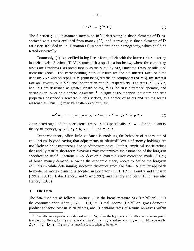
and outside of broad money. The data span the period 1975–1994 and were obtainedfrom the Bank of Greece. All series are quarterly, seasonally unadjusted. The data werenot seasonally adjusted because such pre-filtering may affect short-term dynamics; seeWallis (1974) and Ericsson, Hendry, and Tran (1994). Rather, seasonality is capturedexplicitly in estimation by including seasonal dummies and (initially) seasonal lags in theset of regressors. This subsection sequentially discusses money, prices, income, and therates of return, where the latter are compared with their corresponding assets. Appendix Iconsiders the definition and construction of the data in detail.

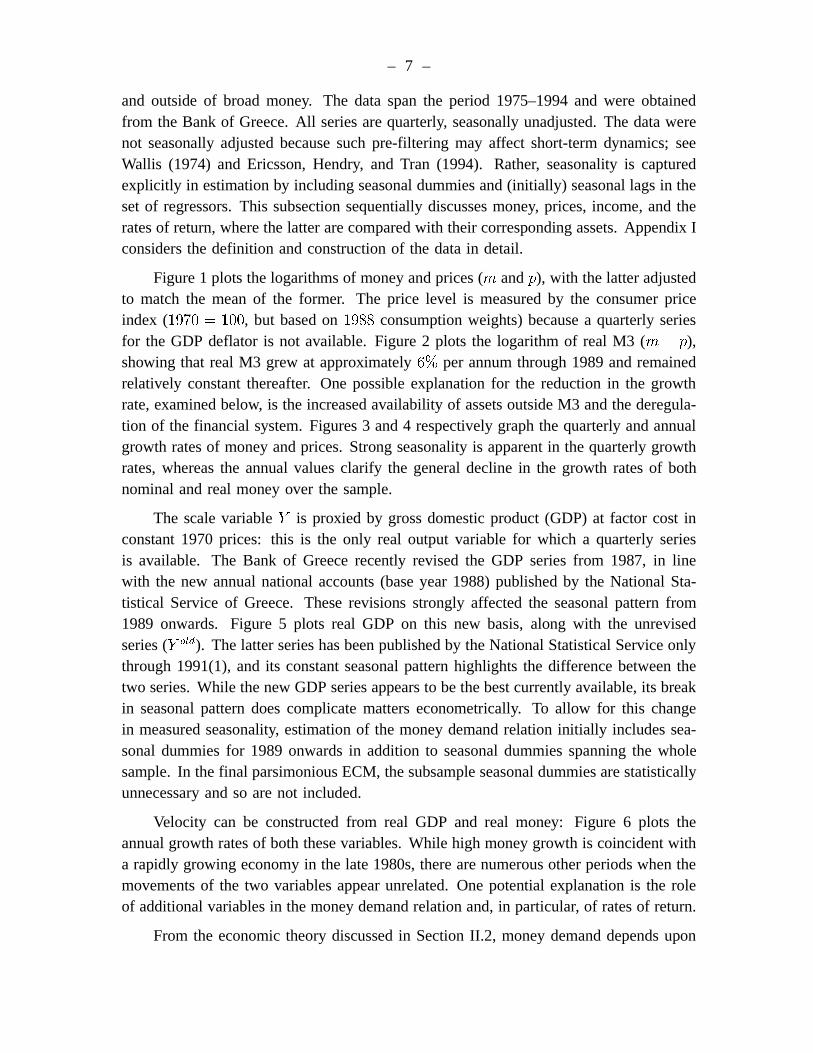
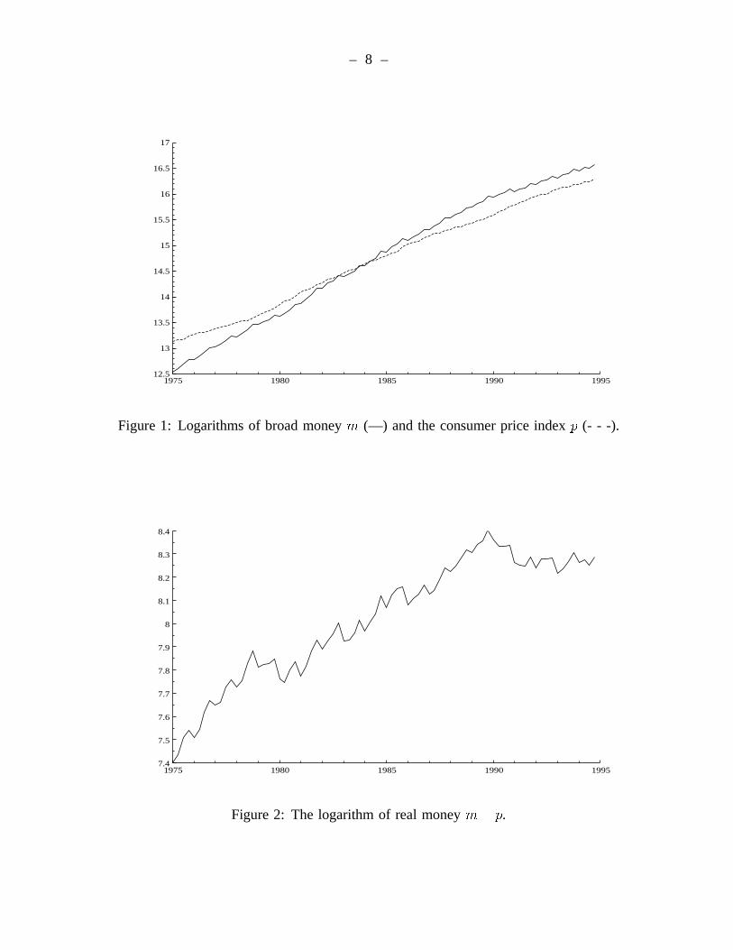
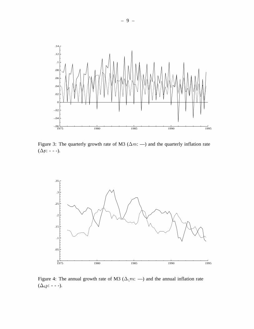
Figure 1 plots the logarithms of money and prices (m andp), with the latter adjustedto match the mean of the former. The price level is measured by the consumer priceindex (1970 = 100, but based on1988 consumption weights) because a quarterly seriesfor the GDP deflator is not available. Figure 2 plots the logarithm of real M3 (m¡ p),showing that real M3 grew at approximately6% per annum through 1989 and remainedrelatively constant thereafter. One possible explanation for the reduction in the growthrate, examined below, is the increased availability of assets outside M3 and the deregula-tion of the financial system. Figures 3 and 4 respectively graph the quarterly and annualgrowth rates of money and prices. Strong seasonality is apparent in the quarterly growthrates, whereas the annual values clarify the general decline in the growth rates of bothnominal and real money over the sample.

The scale variableY is proxied by gross domestic product (GDP) at factor cost inconstant 1970 prices: this is the only real output variable for which a quarterly seriesis available. The Bank of Greece recently revised the GDP series from 1987, in linewith the new annual national accounts (base year 1988) published by the National Sta-tistical Service of Greece. These revisions strongly affected the seasonal pattern from1989 onwards. Figure 5 plots real GDP on this new basis, along with the unrevisedseries (Y old). The latter series has been published by the National Statistical Service onlythrough 1991(1), and its constant seasonal pattern highlights the difference between thetwo series. While the new GDP series appears to be the best currently available, its breakin seasonal pattern does complicate matters econometrically. To allow for this changein measured seasonality, estimation of the money demand relation initially includes sea-sonal dummies for 1989 onwards in addition to seasonal dummies spanning the wholesample. In the final parsimonious ECM, the subsample seasonal dummies are statisticallyunnecessary and so are not included.

Velocity can be constructed from real GDP and real money: Figure 6 plots theannual growth rates of both these variables. While high money growth is coincident witha rapidly growing economy in the late 1980s, there are numerous other periods when themovements of the two variables appear unrelated. One potential explanation is the roleof additional variables in the money demand relation and, in particular, of rates of return.

From the economic theory discussed in Section II.2, money demand depends upon

– 8 –

1975 1980 1985 1990 199512.5

13

13.5

14

14.5

15

15.5

16

16.5

17

Figure 1: Logarithms of broad moneym (—) and the consumer price indexp (- - -).

1975 1980 1985 1990 19957.4

7.5

7.6

7.7

7.8

7.9

8

8.1

8.2

8.3

8.4

Figure 2: The logarithm of real moneym¡ p.

– 9 –

1975 1980 1985 1990 1995-.06

-.04

-.02

0

.02

.04

.06

.08

.1

.12

.14

Figure 3: The quarterly growth rate of M3 (¢m: —) and the quarterly inflation rate(¢p: - - -).

1975 1980 1985 1990 19950

.05

.1

.15

.2

.25

.3

.35

Figure 4: The annual growth rate of M3 (¢4m: —) and the annual inflation rate(¢4p: - - -).

– 10 –

1975 1980 1985 1990 199511.1

11.2

11.3

11.4

11.5

11.6

11.7

11.8

11.9

Figure 5: Logarithms of real GDP on the new basis (y: —) and the old basis(yold: - - -).

1975 1980 1985 1990 1995-.1

-.05

0

.05

.1

.15

Figure 6: The annual growth rates of real M3 [¢4(m¡ p): —] and real GDP(¢4y: - - -).

– 11 –

both own rates of return and outside rates of return. A distinct asset corresponds to eachrate of return, with movements in the rates of return influencing the holdings across thevarious assets. With that in mind, the remainder of this subsection considers variouscompeting assets in Greece and their rates of return.

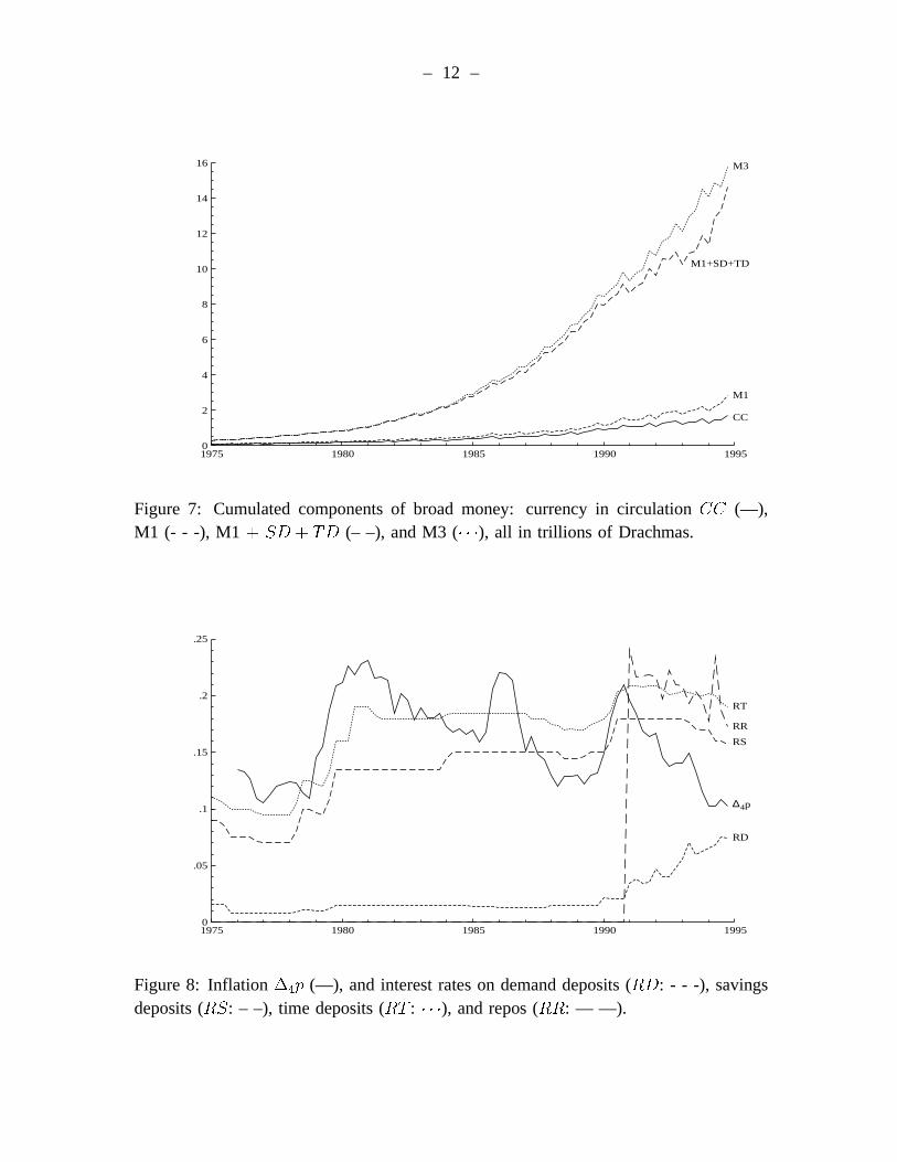
Broad money may be decomposed into several assets, with each asset offering apossibly different (own) rate of return. For Greece, the relevant components of M3 are:currency in circulation (CC), private demand deposits (DD), private savings deposits(SD), time deposits (TD), bank bonds (BB), and repurchase agreements (repos, denotedREP ). Figure 7 graphs these components, cumulatively. Narrow money (M1) is thesum of the first two components (CC +DD), and M3 is the sum of all six components.

Each component of M3 has an associated nominal rate of return: zero for currency,RD for demand deposits,RS for savings accounts,RT for time deposits, andRR forrepos.5 Figure 8 plots the annual rate of inflation¢

4p and the four nonzero rates of

return, where the rates are in percent per annum, expressed as fractions. For much ofthe period until mid-1986, allex postreal interest rates were negative. Thereafter,expost real returns on savings and time deposits were positive, except for a brief interludearound 1990 when inflation again reached20 percent. Repos were introduced in 1990and have offered rates of return competitive with time deposits.

Time deposits and repos offer the highest rates of return on the components of M3described above, soRT andRR are natural proxies for the own (marginal) rate for M3.For that reason, and in order to limit the number of variables examined,RD andRS areexcluded from the econometric analysis in Sections III–V.

One adjustment to rates on components of M3 appears economically and statisticallyimportant. In 1991(1), the government introduced a10 percent withholding tax on interestfrom bank deposits, increasing the tax in mid-1992 to15 percent. In April 1994, this taxwas extended to cover returns from repurchase agreements. Thus, the after-tax returnson these assets (denotedRT n andRRn) seem relevant to individuals’ decisions aboutmoney holdings.6

5 The interest rate on bank bonds is not currently available. However, as Figure 9 below shows, thefraction of bank bonds in M3 changes only very slowly over time and is never greater than 8%.

That said, repos, introduced at the end of 1990, have become an increasingly important source of fundsfor deposit institutions. In 1992, the Bank of Greece redefined M3 to include bank bonds and repos, usingthis new measure to set the M3 targets in its monetary program. We use that new definition of broadmoney for the entire sample period.

6 Changes in the institutional structure and the tax system also could affect the relative returns onexisting and new assets and hence the demand for money. For instance, the efficiency of collection (andthe ease of avoidance) of the withholding tax on interest income could be important. In the United States,such witholding tax is easily avoided, but avoidingeventualpayment of tax on interest income is moredifficult because banks are required to report interest earnings to the Internal Revenue Service.

– 12 –

1975 1980 1985 1990 19950

2

4

6

8

10

12

14

16

CC

M1+SD+TD

M1

M3

Figure 7: Cumulated components of broad money: currency in circulationCC (—),M1 (- - -), M1 + SD + TD (– –), and M3 (¢ ¢ ¢), all in trillions of Drachmas.

1975 1980 1985 1990 19950

.05

.1

.15

.2

.25

RD

RS

RT

RR

∆4p

Figure 8: Inflation¢4p (—), and interest rates on demand deposits (RD: - - -), savingsdeposits (RS: – –), time deposits (RT : ¢ ¢ ¢), and repos (RR: — —).

– 13 –

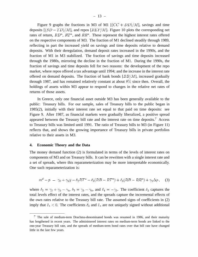
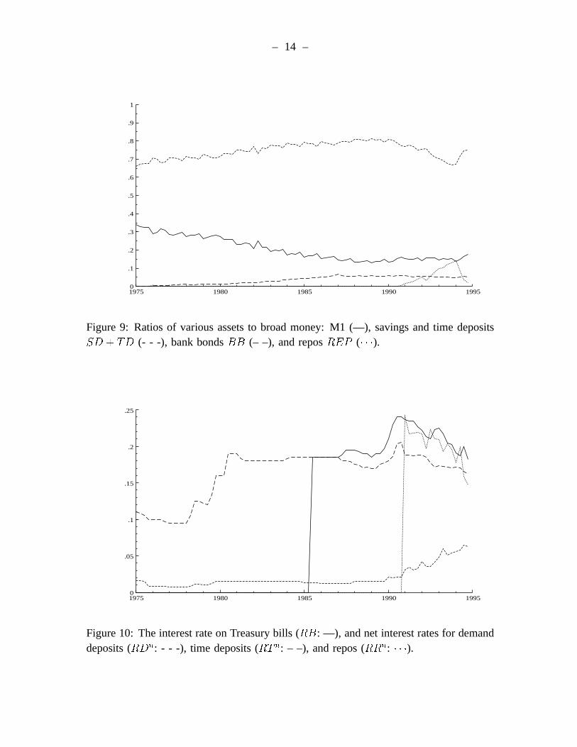
Figure 9 graphs the fractions in M3 of M1 [(CC + DD)=M ], savings and timedeposits [(SD + TD)=M ], and repos [REP=M ]. Figure 10 plots the corresponding netrates of return,RDn, RT n, andRRn. These represent the highest interest rates offeredon the respective components of M3. The fraction of M1 declined steadily through 1989,reflecting in part the increased yield on savings and time deposits relative to demanddeposits. With their deregulation, demand deposit rates increased in the 1990s, and thefraction of M1 in M3 stabilized. The fraction of savings and time deposits increasedthrough the 1980s, mirroring the decline in the fraction of M1. During the 1990s, thefraction of savings and time deposits fell for two reasons: the development of the repomarket, where repos offered a tax advantage until 1994; and the increase in the interest rateoffered on demand deposits. The fraction of bank bonds [BB=M ], increased graduallythrough 1987, and has remained relatively constant at about8% since then. Overall, theholdings of assets within M3 appear to respond to changes in the relative net rates ofreturns of those assets.

In Greece, only one financial asset outside M3 has been generally available to thepublic: Treasury bills. For our sample, sales of Treasury bills to the public began in1985(2), initially with their interest rate set equal to that paid on time deposits: seeFigure 9. After 1987, as financial markets were gradually liberalized, a positive spreadappeared between the Treasury bill rate and the interest rate on time deposits.7 Accessto Treasury bills was limited until 1991. The ratio of Treasury bills to M3 (in Figure 11)reflects that, and shows the growing importance of Treasury bills in private portfoliosrelative to their assets in M3.

4. Economic Theory and the Data

The money demand function (2) is formulated in terms of the levels of interest rates oncomponents of M3 and on Treasury bills. It can be rewritten with a single interest rate anda set of spreads, where this reparameterization may be more interpretable economically.One such reparameterization is:

md¡ p = °

0+ °

1y + ±

2RT n + ±

3(RB ¡RT n) + ±

4(RB ¡RRn) + °

5¢p ; (3)

where±2= °

2+ °

3+ °

4, ±

3= °

3+ °

4, and±

4= ¡°

3. The coefficient±

2captures the

total levels effect of the interest rates, and the spreads capture the incremental effects ofthe own rates relative to the Treasury bill rate. The assumed signs of coefficients in (2)imply that ±

4< 0. The coefficients±

2and±

3are not uniquely signed without additional

7 The sale of medium-term Drachma-denominated bonds was resumed in 1986, and their maturityhas lengthened in recent years. The administered interest rates on medium-term bonds are linked to theone-year Treasury bill rate, and the spreads of medium-term bond rates over that bill rate have changedlittle in the last few years.

– 14 –

1975 1980 1985 1990 19950

.1

.2

.3

.4

.5

.6

.7

.8

.9

1

Figure 9: Ratios of various assets to broad money: M1 (—), savings and time depositsSD + TD (- - -), bank bondsBB (– –), and reposREP (¢ ¢ ¢).

1975 1980 1985 1990 19950

.05

.1

.15

.2

.25

Figure 10: The interest rate on Treasury bills (RB: —), and net interest rates for demanddeposits (RDn: - - -), time deposits (RT n: – –), and repos (RRn: ¢ ¢ ¢).

– 15 –

1975 1980 1985 1990 1995-.05

0

.05

.1

.15

.2

.25

.3

.35

Figure 11: The ratio of outstanding Treasury bills to M3 (—), and the interest-ratespreadsRB ¡RT n (- - -) andRB ¡RRn (– –).

1975 1980 1985 1990 1995-4

-3.9

-3.8

-3.7

-3.6

-3.5

-3.4

-3.3

Figure 12: The logarithm of inverse velocitym¡ p¡ y (—) and the net interest rate ontime depositsRT n (- - -), plotted with matched means and ranges.

– 16 –

information. However, it seems likely that±2> 0 and ±

3< 0, particularly if (for ±

2)

Treasury bills are an imperfect substitute for M3 and if (for±3) the spreadRB¡RT n is

nonzero during some periods whenRB ¡RRn is zero or undefined.

Figure 11 plots the two spreads in (3),(RB¡RT n) and(RB¡RRn). Because theratio of Treasury bills to M3 is small until 1990, we make the simplifying assumptionthat Treasury bills only became available to the public as an alternative to M3 beginningin 1991. Thus, in modeling money demand, the spread(RB¡RT n) in (3) is replaced bya modified spreadST , which is zero through 1990 and(RB ¡ RT n) thereafter. Reposare treated similarly, as follows. Because the fraction of repos in M3 was small duringthe first year that they were available (1991; see Figure 9), we use a modified spreadSR,defined as zero through 1991 and equal to(RB ¡RRn) thereafter. Thus, the empiricalmoney-demand relation is specified as:

md¡ p = °

0+ °

1y + ±

2RT n + ±

3ST + ±

4SR + °

5¢p : (4)

Until virtually the end of the sample, the value of outstanding Treasury bills andrepos is small relative to M3, so a simple representation of (4) involves the return ononly one financial asset, M3 itself. Figure 12 plots this net return (RT n) and measuredinverse velocity. The latter variable is equivalent to imposing a unit income elasticityin (1) (or °

1= 1 in (4)), andRT n is adjusted in the figure so as to match the mean

and range of(m ¡ p ¡ y). While the two series exhibit strong seasonal and dynamicdifferences, their longer-term movements are similar, suggesting possible cointegrationof the two variables. Sections III and IV consider cointegration explicitly.

Foreign-denominated assets represent one additional possible alternative to holdingM3. Their return is captured by the rate of depreciation of the exchange rate plus theinterest rate on the asset. Figure 13 plots the quarterly depreciation rate¢e as well asthe domestic inflation rate¢p, whereE is an index of the nominal effective exchangerate using 1988 trade weights (1970 = 1:00). Notable devaluations occurred in January1983 (of151

2

%) and October 1985 (of20%). In a preliminary analysis, the depreciationrate and foreign interest rates (such as LIBOR) did not appear to matter, except that adummy (denotedDE) for 1982(4)–1983(1) helped capture the apparent anticipation andrealization of the first major devaluation. Various capital controls were in place for muchof the sample, and they may be responsible for the lack of significance of returns onforeign assets. Restrictions on capital movements were significantly liberalized in May1994, and this allowed the use of new financial instruments like synthetic swaps. Becausedata for the returns on synthetic swaps are not currently available, we include a dummy(denotedDS) beginning with their introduction in 1994(3).

– 17 –

1975 1980 1985 1990 1995-.05

0

.05

.1

.15

.2

Figure 13: The quarterly inflation rate¢p (—) and the quarterly depreciation of theexchange rate¢e (- - -).

1985 1986 1987 1988 1989 1990 1991 1992 1993 1994 19950

.1

.2

.3

.4

.5

.6

.7

.8

.9

1

Figure 14: The six recursively estimated eigenvalues.

– 18 –

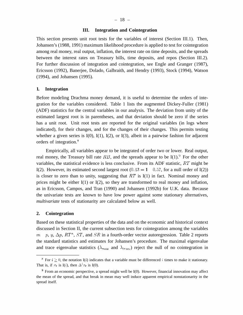
III. Integration and Cointegration

This section presents unit root tests for the variables of interest (Section III.1). Then,Johansen’s (1988, 1991) maximum likelihood procedure is applied to test for cointegrationamong real money, real output, inflation, the interest rate on time deposits, and the spreadsbetween the interest rates on Treasury bills, time deposits, and repos (Section III.2).For further discussion of integration and cointegration, see Engle and Granger (1987),Ericsson (1992), Banerjee, Dolado, Galbraith, and Hendry (1993), Stock (1994), Watson(1994), and Johansen (1995).

1. Integration

Before modeling Drachma money demand, it is useful to determine the orders of inte-gration for the variables considered. Table 1 lists the augmented Dickey-Fuller (1981)(ADF) statistics for the central variables in our analysis. The deviation from unity of theestimated largest root is in parentheses, and that deviation should be zero if the serieshas a unit root. Unit root tests are reported for the original variables (in logs whereindicated), for their changes, and for the changes of their changes. This permits testingwhether a given series is I(0), I(1), I(2), or I(3), albeit in a pairwise fashion for adjacentorders of integration.8

Empirically, all variables appear to be integrated of order two or lower. Real output,real money, the Treasury bill rateRB, and the spreads appear to be I(1).9 For the othervariables, the statistical evidence is less conclusive. From its ADF statistic,RT might beI(2). However, its estimated second largest root (0:43 = 1¡0:57, for a null order of I(2))is closer to zero than to unity, suggesting thatRT is I(1) in fact. Nominal money andprices might be either I(1) or I(2), so they are transformed to real money and inflation,as in Ericsson, Campos, and Tran (1990) and Johansen (1992b) for U.K. data. Becausethe univariate tests are known to have low power against some stationary alternatives,multivariate tests of stationarity are calculated below as well.

2. Cointegration

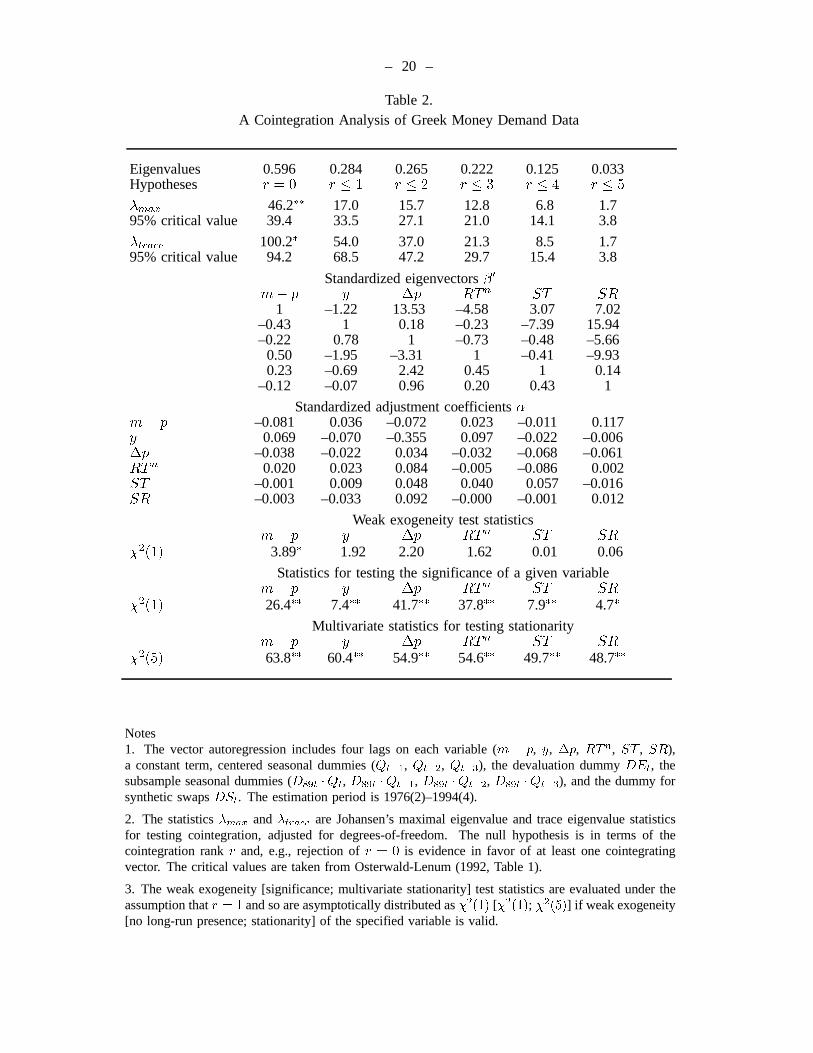
Based on these statistical properties of the data and on the economic and historical contextdiscussed in Section II, the current subsection tests for cointegration among the variablesm¡p, y, ¢p, RT n, ST , andSR in a fourth-order vector autoregression. Table 2 reportsthe standard statistics and estimates for Johansen’s procedure. The maximal eigenvalueand trace eigenvalue statistics (¸max and ¸trace) reject the null of no cointegration in

8 For i ¸ 0, the notation I(i) indicates that a variable must be differencedi times to make it stationary.That is, if xt is I(i), then¢ixt is I(0).

9 From an economic perspective, a spread might well be I(0). However, financial innovation may affectthe mean of the spread, and that break in mean may well induce apparent empirical nonstationarity in thespread itself.

– 19 –

Table 1.ADF(4) Statistics for Testing for a Unit Root

Variable

Null Order m p y m¡ p RT RB ST SR

I(1)1:25(0:02)

¡1:51(¡0:04)

¡2:54(¡0:34)

¡1:51(¡0:06)

¡1:93(¡0:07)

¡1:74(¡0:11)

¡1:90(¡0:16)

¡0:35(¡0:13)

I(2)¡3:39+

(¡0:57)¡2:31(¡0:35)

¡4:13¤¤

(¡2:09)¡3:87¤

(¡0:74)¡2:64(¡0:57)

¡3:66¤

(¡1:03)¡5:22¤¤

(¡1:77)¡6:49¤¤

(¡6:32)

I(3)¡5:09¤¤

(¡2:15)¡4:73¤¤

(¡2:49)¡8:15¤¤

(¡6:35)¡4:55¤¤

(¡2:14)¡4:78¤¤

(¡2:64)¡6:13¤¤

(¡3:43)¡7:25¤¤

(¡3:82)¡3:47+

(¡5:17)

Notes1. For a given variable and null order, two values are reported: the fourth-order augmented Dickey-Fuller(1981) statistic, denoted ADF(4); and (in parentheses) the estimated coefficient on the lagged variable,where that coefficient should be zero under the null hypothesis. A constant term, quarterly dummies, anda trend are included in the corresponding regressions. The maximum available sample is used, and variesacross the null order.

2. For any variablex and a null order of I(1), the ADF(4) statistic is testing a null hypothesis of a unitroot in x against an alternative of a stationary root. For a null order of I(2) [I(3)], the statistic is testing anull hypothesis of a unit root in¢x [¢2x] against an alternative of a stationary root in¢x [¢2x].

3. Here and elsewhere in this paper, the superscripts+, *, and ** denote rejection at the 10%, 5%, and1% critical values. The critical values for this table are from MacKinnon (1991).

– 20 –

Table 2.A Cointegration Analysis of Greek Money Demand Data

Eigenvalues 0.596 0.284 0.265 0.222 0.125 0.033Hypotheses r = 0 r · 1 r · 2 r · 3 r · 4 r · 5

¸max 46.2¤¤ 17.0 15.7 12.8 6.8 1.795% critical value 39.4 33.5 27.1 21.0 14.1 3.8

¸trace 100.2¤ 54.0 37.0 21.3 8.5 1.795% critical value 94.2 68.5 47.2 29.7 15.4 3.8

Standardized eigenvectors0

m¡ p y ¢p RTn ST SR1 –1.22 13.53 –4.58 3.07 7.02

–0.43 1 0.18 –0.23 –7.39 15.94–0.22 0.78 1 –0.73 –0.48 –5.66

0.50 –1.95 –3.31 1 –0.41 –9.930.23 –0.69 2.42 0.45 1 0.14

–0.12 –0.07 0.96 0.20 0.43 1

Standardized adjustment coefficients®m¡ p –0.081 0.036 –0.072 0.023 –0.011 0.117y 0.069 –0.070 –0.355 0.097 –0.022 –0.006¢p –0.038 –0.022 0.034 –0.032 –0.068 –0.061RTn 0.020 0.023 0.084 –0.005 –0.086 0.002ST –0.001 0.009 0.048 0.040 0.057 –0.016SR –0.003 –0.033 0.092 –0.000 –0.001 0.012

Weak exogeneity test statisticsm¡ p y ¢p RTn ST SR

Â2(1) 3.89¤ 1.92 2.20 1.62 0.01 0.06

Statistics for testing the significance of a given variablem¡ p y ¢p RTn ST SR

Â2(1) 26.4¤¤ 7.4¤¤ 41.7¤¤ 37.8¤¤ 7.9¤¤ 4.7¤

Multivariate statistics for testing stationaritym¡ p y ¢p RTn ST SR

Â2(5) 63.8¤¤ 60.4¤¤ 54.9¤¤ 54.6¤¤ 49.7¤¤ 48.7¤¤

Notes1. The vector autoregression includes four lags on each variable (m ¡ p, y, ¢p, RTn, ST , SR),a constant term, centered seasonal dummies (Qt¡1, Qt¡2, Qt¡3), the devaluation dummyDEt, thesubsample seasonal dummies (D89t ¢Qt, D89t ¢Qt¡1, D89t ¢Qt¡2, D89t ¢Qt¡3), and the dummy forsynthetic swapsDSt. The estimation period is 1976(2)–1994(4).

2. The statistics max and¸trace are Johansen’s maximal eigenvalue and trace eigenvalue statisticsfor testing cointegration, adjusted for degrees-of-freedom. The null hypothesis is in terms of thecointegration rankr and, e.g., rejection ofr = 0 is evidence in favor of at least one cointegratingvector. The critical values are taken from Osterwald-Lenum (1992, Table 1).

3. The weak exogeneity [significance; multivariate stationarity] test statistics are evaluated under theassumption thatr = 1 and so are asymptotically distributed asÂ2(1) [Â2(1); Â2(5)] if weak exogeneity[no long-run presence; stationarity] of the specified variable is valid.

– 21 –

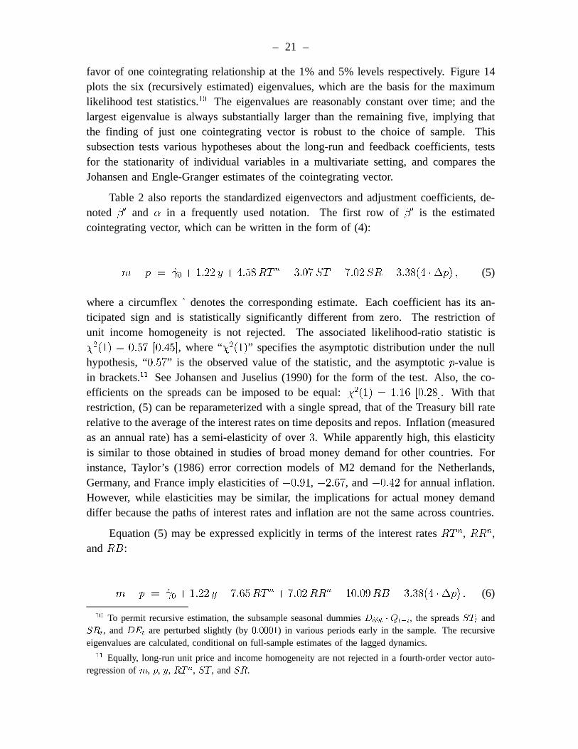
favor of one cointegrating relationship at the 1% and 5% levels respectively. Figure 14plots the six (recursively estimated) eigenvalues, which are the basis for the maximumlikelihood test statistics.10 The eigenvalues are reasonably constant over time; and thelargest eigenvalue is always substantially larger than the remaining five, implying thatthe finding of just one cointegrating vector is robust to the choice of sample. Thissubsection tests various hypotheses about the long-run and feedback coefficients, testsfor the stationarity of individual variables in a multivariate setting, and compares theJohansen and Engle-Granger estimates of the cointegrating vector.

Table 2 also reports the standardized eigenvectors and adjustment coefficients, de-noted ¯0 and ® in a frequently used notation. The first row of¯ 0 is the estimatedcointegrating vector, which can be written in the form of (4):

m¡ p = °0+ 1:22 y + 4:58RT n

¡ 3:07ST ¡ 7:02SR¡ 3:38(4 ¢¢p) ; (5)

where a circumflex denotes the corresponding estimate. Each coefficient has its an-ticipated sign and is statistically significantly different from zero. The restriction ofunit income homogeneity is not rejected. The associated likelihood-ratio statistic isÂ2(1) = 0:57 [0:45], where “Â2(1)” specifies the asymptotic distribution under the nullhypothesis, “0:57” is the observed value of the statistic, and the asymptoticp-value isin brackets.11 See Johansen and Juselius (1990) for the form of the test. Also, the co-efficients on the spreads can be imposed to be equal:Â2(1) = 1:16 [0:28]. With thatrestriction, (5) can be reparameterized with a single spread, that of the Treasury bill raterelative to the average of the interest rates on time deposits and repos. Inflation (measuredas an annual rate) has a semi-elasticity of over3. While apparently high, this elasticityis similar to those obtained in studies of broad money demand for other countries. Forinstance, Taylor’s (1986) error correction models of M2 demand for the Netherlands,Germany, and France imply elasticities of¡0:91, ¡2:67, and¡0:42 for annual inflation.However, while elasticities may be similar, the implications for actual money demanddiffer because the paths of interest rates and inflation are not the same across countries.

Equation (5) may be expressed explicitly in terms of the interest ratesRT n, RRn,andRB:

m¡ p = °0+ 1:22 y + 7:65RT n + 7:02RRn

¡ 10:09RB ¡ 3:38(4 ¢¢p) : (6)

10 To permit recursive estimation, the subsample seasonal dummiesD89t ¢ Qt¡i, the spreadsSTt andSRt, andDEt are perturbed slightly (by0:0001) in various periods early in the sample. The recursiveeigenvalues are calculated, conditional on full-sample estimates of the lagged dynamics.

11 Equally, long-run unit price and income homogeneity are not rejected in a fourth-order vector auto-regression ofm, p, y, RTn, ST , andSR.

– 22 –

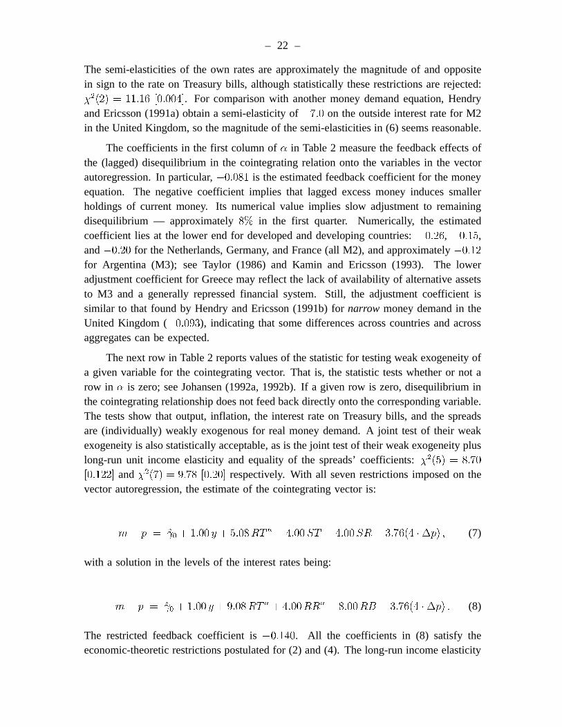
The semi-elasticities of the own rates are approximately the magnitude of and oppositein sign to the rate on Treasury bills, although statistically these restrictions are rejected:Â2(2) = 11:16 [0:004]. For comparison with another money demand equation, Hendryand Ericsson (1991a) obtain a semi-elasticity of¡7:0 on the outside interest rate for M2in the United Kingdom, so the magnitude of the semi-elasticities in (6) seems reasonable.

The coefficients in the first column of® in Table 2 measure the feedback effects ofthe (lagged) disequilibrium in the cointegrating relation onto the variables in the vectorautoregression. In particular,¡0:081 is the estimated feedback coefficient for the moneyequation. The negative coefficient implies that lagged excess money induces smallerholdings of current money. Its numerical value implies slow adjustment to remainingdisequilibrium — approximately8% in the first quarter. Numerically, the estimatedcoefficient lies at the lower end for developed and developing countries:¡0:26, ¡0:15,and¡0:20 for the Netherlands, Germany, and France (all M2), and approximately¡0:12

for Argentina (M3); see Taylor (1986) and Kamin and Ericsson (1993). The loweradjustment coefficient for Greece may reflect the lack of availability of alternative assetsto M3 and a generally repressed financial system. Still, the adjustment coefficient issimilar to that found by Hendry and Ericsson (1991b) fornarrow money demand in theUnited Kingdom (¡0:093), indicating that some differences across countries and acrossaggregates can be expected.

The next row in Table 2 reports values of the statistic for testing weak exogeneity ofa given variable for the cointegrating vector. That is, the statistic tests whether or not arow in ® is zero; see Johansen (1992a, 1992b). If a given row is zero, disequilibrium inthe cointegrating relationship does not feed back directly onto the corresponding variable.The tests show that output, inflation, the interest rate on Treasury bills, and the spreadsare (individually) weakly exogenous for real money demand. A joint test of their weakexogeneity is also statistically acceptable, as is the joint test of their weak exogeneity pluslong-run unit income elasticity and equality of the spreads’ coefficients:Â2(5) = 8:70

[0:122] andÂ2(7) = 9:78 [0:20] respectively. With all seven restrictions imposed on thevector autoregression, the estimate of the cointegrating vector is:

m¡ p = °0+ 1:00 y + 5:08RT n

¡ 4:00ST ¡ 4:00SR¡ 3:76(4 ¢¢p) ; (7)

with a solution in the levels of the interest rates being:

m¡ p = °0+ 1:00 y + 9:08RT n + 4:00RRn

¡ 8:00RB ¡ 3:76(4 ¢¢p) : (8)

The restricted feedback coefficient is¡0:140. All the coefficients in (8) satisfy theeconomic-theoretic restrictions postulated for (2) and (4). The long-run income elasticity

– 23 –

is unity, coefficients on the own rates are positive, those on the outside rate and inflationare negative, and those on the spreads (in (7)) are negative.

Valid weak exogeneity permits analysis of the cointegrating vector in a single-equation conditional error correction model of money without loss of information, soSection IV turns to single equation modeling. The remainder of the current section con-siders significance tests of the variables in the cointegrating vector and multivariate testsof unit roots, and it compares the cointegration results in Table 2 with those from theEngle-Granger procedure.

The penultimate row of Table 2 reports chi-squared statistics for testing the signif-icance of individual variables in the cointegrating vector. Each variable is significant atthe 5% level, and all but one (SR) are significant at the1% level.

The final row of Table 2 reports values of a multivariate statistic for testing thestationarity of a given variable. This statistic tests the restriction that the cointegratingvector contains all zeros except for a unity corresponding to the designated variable,where the test is conditional on there being one cointegrating vector. For instance, the nullhypothesis of stationary real money implies that the cointegrating vector is(1 0 0 0 0 0)0.Empirically, all the tests reject stationarity withp-values of less than0:01%. By beingmultivariate and so involving a larger information set, these statistics may have higherpower than their univariate counterparts in Table 1. Also, the null hypothesis is thestationarity of a given variable rather than the nonstationarity thereof, and that may bemore appealing. That said, these rejections of stationarity are in line with theinability inTable 1 to reject the null hypothesis of a unit root in each of these variables.

Engle and Granger’s (1987) procedure is another popular approach for testing coin-tegration and for estimating the cointegrating vector. The Johansen and Engle-Grangerprocedures embody different assumptions about dynamics, so it is useful to compareresults from both techniques. In the Engle-Granger procedure, the long-run relationshipin (2) is estimated without regard to short-term dynamics, and the residuals from thisregression are tested for stationarity. If the residuals are stationary, then (2) represents acointegrating relationship.

This procedure, though simple, may have poor finite-sample properties because itgenerally does not use all available information on dynamics efficiently; see Banerjee,Dolado, Hendry, and Smith (1986) and Kremers, Ericsson, and Dolado (1992). Forcomparison with (5) and (7) [and (10) and (14) below], the static regression for theEngle-Granger procedure is:

– 24 –

m¡ p = °0+ 2:25 y + 0:28RT n

¡ 3:46ST + 1:17SR¡ 0:44(4 ¢¢p)

T = 74 [1976(3)¡ 1994(4)] R2 = 0:945 ¾ = 5:79% dw = 0:87

ADF (4) = ¡2:50 ADF (0) = ¡4:46 :

(9)

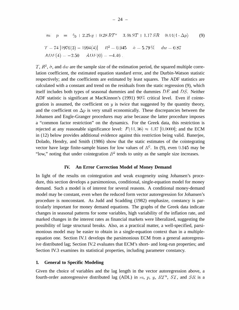
T , R2, ¾, anddw are the sample size of the estimation period, the squared multiple corre-lation coefficient, the estimated equation standard error, and the Durbin-Watson statisticrespectively; and the coefficients are estimated by least squares. The ADF statistics arecalculated with a constant and trend on the residuals from the static regression (9), whichitself includes both types of seasonal dummies and the dummiesDE andDS. NeitherADF statistic is significant at MacKinnon’s (1991)90% critical level. Even if cointe-gration is assumed, the coefficient ony is twice that suggested by the quantity theory,and the coefficient on¢p is very small economically. These discrepancies between theJohansen and Engle-Granger procedures may arise because the latter procedure imposesa “common factor restriction” on the dynamics. For the Greek data, this restriction isrejected at any reasonable significance level:F (44; 36) ¼ 4:37 [0:0000]; and the ECMin (12) below provides additional evidence against this restriction being valid. Banerjee,Dolado, Hendry, and Smith (1986) show that the static estimates of the cointegratingvector have large finite-sample biases for low values ofR2. In (9), even0:945 may be“low,” noting that under cointegrationR2 tends to unity as the sample size increases.

IV. An Error Correction Model of Money Demand

In light of the results on cointegration and weak exogeneity using Johansen’s proce-dure, this section develops a parsimonious, conditional, single-equation model for moneydemand. Such a model is of interest for several reasons. A conditional money-demandmodel may be constant, even when the reduced form vector autoregression for Johansen’sprocedure is nonconstant. As Judd and Scadding (1982) emphasize, constancy is par-ticularly important for money demand equations. The graphs of the Greek data indicatechanges in seasonal patterns for some variables, high variability of the inflation rate, andmarked changes in the interest rates as financial markets were liberalized, suggesting thepossibility of large structural breaks. Also, as a practical matter, a well-specified, parsi-monious model may be easier to obtain in a single-equation context than in a multiple-equation one. Section IV.1 develops the parsimonious ECM from a general autoregress-ive distributed lag; Section IV.2 evaluates that ECM’s short- and long-run properties; andSection IV.3 examines its statistical properties, including parameter constancy.

1. General to Specific Modeling

Given the choice of variables and the lag length in the vector autoregression above, afourth-order autoregressive distributed lag (ADL) inm, p, y, RT n, ST , andSR is a

– 25 –

natural starting point for single-equation modeling. Paralleling the vector autoregression,this model was extended in three ways. First, the dummy variableDE for 1982(4)–1983(1) was included to account for fluctuations in money demand associated with the151

2

percent devaluation of the Drachma in early January 1983. Second, the dummyvariableDS was included to proxy for the returns on synthetic swaps. Third, fourseasonal dummies beginning in 1989 were included so as to allow for the change inseasonality of measured GDP. This subsection estimates that autoregressive distributedlag, solves for its long-run properties, reinterprets it as an unrestricted ECM, and reducesit to a parsimonious ECM.

The long-run static solution to the estimated autoregressive distributed lag is:

m = ¡ 4:31(5:69)

+ 1:01(0:11)

p + 1:04(0:52)

y + 4:56(2:59)

RT n¡ 3:87(1:29)

ST ¡ 7:05(5:22)

SR :

T = 75 [1976(2)¡ 1994(4)] :

(10)

The coefficients onp andy are numerically close to unity, and each is much less than astandard deviation away from unity, so the long-run solution to the ADL could likely beformulated in terms of the inverse velocity. Additionally, the coefficients onRT n, ST ,andSR are similar to the system estimates in (5), providing further (indirect) evidenceof the validity of weak exogeneity.

Autoregressive distributed lags have error correction representations. Thus, the long-run money demand relation (2) can be explicitly embedded in the ADL model, writtenas an ECM:

¢mt =kP

i=1

µ1i¢mt¡i +

kP

i=0

µ2i¢pt¡i +

kP

i=0

µ3i¢yt¡i

+kP

i=0

µ4i¢RT

nt¡i +

kP

i=0

µ5i¢STt¡i +

kP

i=0

µ6i¢SRt¡i

+ µ7(m¡m¤)t¡1 +

3P

i=0

(µ8iQt¡i + µ

9iD89tQt¡i) + µ00Dt + "t : (11)

The lag lengthk is 3; coefficients are denoted byµj (or µji if lags are involved);m¤ is thedesired nominal money stock obtained from (2);fQt¡ig are centered seasonal dummies,except thatQt is the constant term;D

89t is a step dummy, being zero through 1988and unity from 1989(1) onwards;Dt is the vector(DE;DS)0t; and "t is the equation’serror. The model has a flexible lag structure, yet yields the static equilibrium (2) whengrowth rates (including¢p) are set to zero. The “error correction” term(m ¡m¤)t¡1

– 26 –

corresponds to the disequilibrium from the long-run solution, with money adjusting insubsequent periods ifµ

7< 0.

The ECM generalizes the traditional partial adjustment model, allowing for differ-ent speeds of reaction to the different determinants of money demand, yet through theerror correction term ensures that the long-run relationship holds in steady state. Thespecification in (11) is also related to a theory of “inventory adjustment,” in which short-run factors determine fluctuations of money holdings within given bands, while long-runfactors influence the level of the bands themselves. See Miller and Orr (1966), Akerlof(1979), Akerlof and Milbourne (1980), Milbourne (1983), and Smith (1986). Equally,the ECM is a re-parameterization of a general autoregressive distributed-lag model in(log) levels. The ECM formulation is attractive in that it immediately provides the para-meter describing the rate of short-run adjustment to disequilibrium. See de Brouwerand Ericsson (1995) for an extended expository discussion of the relationship betweenautoregressive distributed lags, ECMs, and their long-run solutions.

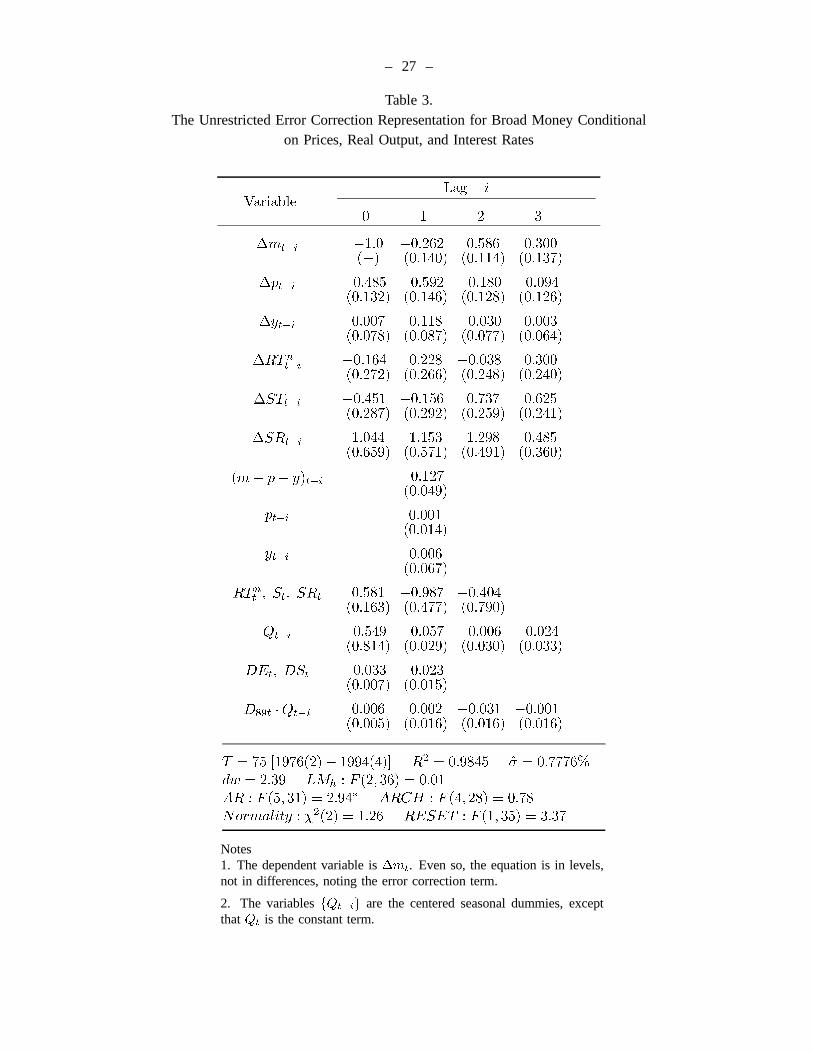
Table 3 lists the estimated coefficients, standard errors, and test statistics for theECM representation in (11), which is our starting point for the general-to-specific model-ing of Greek money demand. The coefficient on the error correction term(m¡p¡y)t¡1is ¡0:127, close to that obtained by Johansen’s procedure. Likewise, the estimatedcoefficients onpt¡1 and yt¡1 are close to zero, both numerically and statistically, im-plying that the hypothesis of long-run unit price and income homogeneity imbedded in(m ¡ p ¡ y)t¡1 is reasonable. Formally, the restriction of long-run price and incomehomogeneity is not rejected (LMh).

Table 3 and the regressions below include diagnostic statistics for testing against var-ious alternative hypotheses: residual autocorrelation (dw andAR), skewness and excesskurtosis (Normality), autoregressive conditional heteroscedasticity (ARCH), RESET(RESET ), heteroscedasticity (Hetero), heteroscedasticity quadratic in the regressors(alternatively, functional form mis-specification) (Form), non-innovation errors relativeto a more general model (Inn), and predictive failure (Chow, Chow’s prediction intervalstatistic).12 The null distribution is designated byÂ2(¢) or F (¢; ¢), the degrees of free-dom fill the parentheses, and (forAR andARCH) the lag order is the first degree offreedom. Statistically, the ADL appears reasonably well specified, with the exception ofsome autocorrelation that is possibly due to the considerable over-parameterization of theunrestricted ADL.

The unrestricted ADL is valuable for obtaining the long-run solution (10), but it

12 For references on the test statistics, see Durbin and Watson (1950, 1951), Box and Pierce (1970),Godfrey (1978), and Harvey (1981, p. 173); Jarque and Bera (1980) and Doornik and Hansen (1994);Engle (1982); Ramsey (1969); White (1980, p. 825) and Nicholls and Pagan (1983) (the latter two on bothHetero andForm); and Chow (1960). The PcGive manual, Doornik and Hendry (1994), also providesextensive discussions of these statistics.

– 27 –

Table 3.The Unrestricted Error Correction Representation for Broad Money Conditional

on Prices, Real Output, and Interest Rates

Lag iVariable

0 1 2 3

¢mt¡i ¡1:0(¡)

¡0:262(0:140)

0:586(0:114)

0:300(0:137)

¢pt¡i ¡0:485(0:132)

¡0:592(0:146)

¡0:180(0:128)

¡0:094(0:126)

¢yt¡i 0:007(0:078)

0:118(0:087)

¡0:030(0:077)

0:003(0:064)

¢RTnt¡i

¡0:164(0:272)

0:228(0:266)

¡0:038(0:248)

0:300(0:240)

¢STt¡i ¡0:451(0:287)

¡0:156(0:292)

0:737(0:259)

0:625(0:241)

¢SRt¡i 1:044(0:659)

1:153(0:571)

1:298(0:491)

0:485(0:360)

(m¡ p¡ y)t¡i ¡0:127(0:049)

pt¡i 0:001(0:014)

yt¡i 0:006(0:067)

RTnt; St; SRt 0:581

(0:163)¡0:987(0:477)

¡0:404(0:790)

Qt¡i ¡0:549(0:814)

¡0:057(0:029)

¡0:006(0:030)

¡0:024(0:033)

DEt; DSt ¡0:033(0:007)

¡0:023(0:015)

D89t ¢Qt¡i 0:006(0:005)

0:002(0:016)

¡0:031(0:016)

¡0:001(0:016)

T = 75 [1976(2)¡ 1994(4)] R2 = 0:9845 ¾ = 0:7776%dw = 2:39 LMh : F (2; 36) = 0:01AR : F (5; 31) = 2:94¤ ARCH : F (4; 28) = 0:78Normality : Â2(2) = 1:26 RESET : F (1; 35) = 3:37

Notes1. The dependent variable is¢mt. Even so, the equation is in levels,not in differences, noting the error correction term.

2. The variablesfQt¡ig are the centered seasonal dummies, exceptthatQt is the constant term.

– 28 –

has far too many parameters for many other uses. While no rules guarantee obtaining asuccessful parsimonious model from the ADL, some intuitive guidelines seemed helpfulin simplification. First, the variablesm, p, y, RT n, ST , andSR were transformed tocurrent and lagged differences and one (possibly lagged) level, as in Table 3. In addition,mt¡1, pt¡1, and yt¡1 were transformed to the differential(m ¡ p ¡ y)t¡1 and the twolog-levels,pt¡1 andyt¡1, thereby reparameterizing these variables as the error correctionterm and two possibly redundant lags. Combined, the two types of transformations helpedobtain a relatively orthogonal set of regressors, making interpretation and simplificationeasier. Second, shorter lag lengths were preferred to longer ones. Third, because oftheir economic importance, variables directly involved in the long-run solution were notdeleted. See Ericsson, Campos, and Tran (1990), Hendry and Ericsson (1991a, 1991b),and Hendry (1995) for more discussion on reparameterizations and general-to-specificmodeling.

Having applied the transformations above and following these informal guidelines,the model in Table 3 could be simplified to the following parsimonious, economicallyinterpretable, and statistically acceptable ECM. Appendix II describes the simplificationpath in greater detail.

¢mt = ¡ 0:117(0:071)[0:078]

¢mt¡1 + 0:671(0:075)[0:095]

¢mt¡2 ¡ 0:394(0:059)[0:066]

¢2pt

+ 0:072(0:024)[0:030]

¢yt ¡ 0:488(0:149)[0:320]

¢STt + 0:603(0:107)[0:140]

¢2STt¡2 ¡ 0:026

(0:006)[0:012]

DEt

¡ 0:086(0:011)[0:013]

(m¡ p¡ y)t¡1 + 0:410(0:053)[0:061]

RT nt ¡ 0:675

(0:140)[0:171]

St

¡ 0:320(0:042)[0:052]

¡ 0:060(0:007)[0:008]

Qt¡1 ¡ 0:040(0:007)[0:008]

Qt¡2 ¡ 0:003(0:008)[0:009]

Qt¡3 (12)

T = 75 [1976(2)¡ 1994(4)] R2 = 0:9712 ¾ = 0:8128% DW = 2:30

AR(5; 56) = 2:04 ARCH : F (4; 53) = 0:57

Normality : Â2(2) = 0:85 RESET : F (1; 60) = 0:71

Hetero : F (22; 38) = 0:44 Inn : F (25; 36) = 1:23 :

Ordinary equation standard errors appear in parentheses( ¢ ); White (1980) and Mac-Kinnon and White’s (1985) heteroscedasticity consistent standard errors appear in squarebrackets[ ¢ ]; and S is (ST + SR)=2, the average of the two spreads, and so is alsoRB¡ (RT n+RRn)=2. Without loss of generality, (12) can be written in a form similarto (11) but with¢(m¡ p)t as the dependent variable, in which case the error correctionterm is:

– 29 –

¡0:086 [m¡ p¡ y ¡ 4:77RT n + 7:85S + 3:59(4 ¢¢p)]t¡1 ; (13)

see Hendry and Ericsson (1991b, equation (15)).

2. Short- and Long-run Properties of the Model

Both short- and long-run properties can be derived from (12). The coefficient on the errorcorrection term is highly significant statistically, establishing that a long-run (cointegrat-ing) relationship exists between broad money, prices, real output, the net interest rate ontime deposits, and the spreads. The size of this coefficient suggests that the adjustmentto disequilibria via the error correction term is slow. The mean lags forp, y, RT n, ST ,andSR are19, 5, 5, 8, and5 quarters respectively; their median lags are all somewhatshorter, being12, 5, 4, 7, and4 quarters respectively.13 In (12), current inflation has anegative and numerically small coefficient, implying that in essence the ECM is model-ing ¢mt in the short run, although real money (and velocity) is being determined in thelong run through the error correction term. Such a relationship is consistent withSs-typemodels of money demand, in which short-run factors determine movements in nominalmoney given desired bands, and longer-run factors (including the price level) determinethe bands themselves.

The solved static long-run money demand function from (12) is:

(m¡ p)s = ¡3:72 + y + 4:77RT n¡ 7:85S : (14)

This long-run relationship between inverse velocity and (for the most part)RT n is visuallyapparent in Figure 12 above, noting thatS = 0 until 1991. Long-run unit elasticities forprices and output are not rejected; and the estimated semi-elasticity of the nominal (net)interest rate on time deposits is4:77, implying an elasticity of about0:7 when annualinterest rates are15 percent.

Other steady-state solutions also can be derived. For example, if money and pricesare assumed to grow at the same rate (¢m = ¢p ´ g), the dynamic steady-state solutionis:

(m¡ p)d = ¡3:72 + y + 4:77RT n¡ 7:85S ¡ 3:59(4 g) ; (15)

13 For computational convenience, the mean and median lags were calculated by estimating equation(12) without imposing long-run unit income and price elasticities, long-run equality of elasticities forST andSR, equal coefficients on¢pt and¢pt¡1, and equal coefficients with opposite sign forSTt¡2andSTt¡4. Because these restrictions are empirically acceptable and the corresponding coefficients areprecisely estimated, the derived mean and median lags from the less restricted equation should not differmuch from those for (12).

– 30 –

where4 g is the annualized nominal growth rate. From (15), inverse velocity in such asteady state depends negatively on the inflation rate, positively on the own rate of return,and negatively on the defined spread. Given the limited range of financial assets availableand the underdeveloped nature of the capital market, real assets have been and are animportant component of an investor’s portfolio. To the extent that the rate of inflationreflects the rate of return on real assets, it is an important determinant of the demand formoney.

Equations (5), (7), (10), and (14) (equally, (15)) present estimates of the long-runmoney demand relation under somewhat different assumptions. Equations (7), (10),and (14) assume weak exogeneity, with (14) also relying on a valid simplification fromTable 3. Equation (5) does not assume weak exogeneity, but its estimates may be moresensitive than (10) and (14) to mis-specification in the equations for income, inflation,and the interest rates. That said, all four estimated long-run solutions are remarkablysimilar, as are their corresponding feedback coefficients for the money equation. Suchrobustness is an argument in favor of the validity of both weak exogeneity and theadditional simplifications entailed by (12) relative to Table 3.

Another fruitful comparison is of the static solution (14), the dynamic steady state(15), and actual real money holdings(m¡ p). Figure 15 plots all three, where the right-hand side variables in (14) and (15) are evaluated at current values, albeit with incomeand inflation as annual averages in order to remove the pronounced seasonality in thosevariables. The static equilibrium path consistently lies above actual real money. Thisdiscrepancy reflects the uniformly positive inflation rate over the sample, which contrastswith the zero inflation rate assumed in the static solution. By comparison, real money andthe dynamic steady state are quite similar: deviations between them are typically10%

and never more than25%, with deviations lasting a year or two at a time; see Figure 16.By comparison, Ericsson, Hendry, and Tran (1994) find that disequilibria in U.K.narrowmoney holdings over roughly the same sample are often more than25% and sometimeseven exceed50%. Such large disequilibria probably reflect the small costs of being outof equilibrium as much as the size of the shocks that created the disequilibria; cf. Hendry(1995, p. 582).

3. Statistical Properties of the Model

Statistically, the ECM in (12) appears reasonably well specified. The restrictions in (12)are not rejected relative to the unrestricted ECM in Table 3 (Inn), and no diagnostic testis significant. Lagrange multiplier tests for a variety of omitted variables in (12) are like-wise not rejected. Specifically,F -statistics for testing the significance offRDn

t¡i; i =

0; : : : ; 4g, fRSn

t¡i; i = 0; : : : ; 4g, fe

t¡i; i = 0; : : : ; 4g, DS

t, and fD89t ¢ Qt¡i

; i =

0; : : : ; 3g are F (5; 56) = 1:51 [0:20], F (5; 56) = 0:24 [0:94], F (5; 56) = 0:31 [0:90],F (1; 60) = 0:89 [0:35], andF (4; 57) = 1:52 [0:21] respectively; and a test of their joint

– 31 –

1975 1980 1985 1990 19957.4

7.6

7.8

8

8.2

8.4

8.6

8.8

9

Figure 15: Actual real money(m¡ p) (—), the static solution(m¡ p)s (- - -), and thedynamic solution(m¡ p)d (– –).

1975 1980 1985 1990 1995-1

-.9

-.8

-.7

-.6

-.5

-.4

-.3

-.2

-.1

0

.1

.2

.3

Figure 16: Deviations between money and the static solution(m¡ p)¡ (m¡ p)s (- - -)and between money and the dynamic solution(m¡ p)¡ (m¡ p)d (– –).

– 32 –

significance yieldsF (20; 41) = 0:86 [0:64]. The variablesRDn andRSn are the interestrates on demand deposits and savings deposits, net of withholding tax.

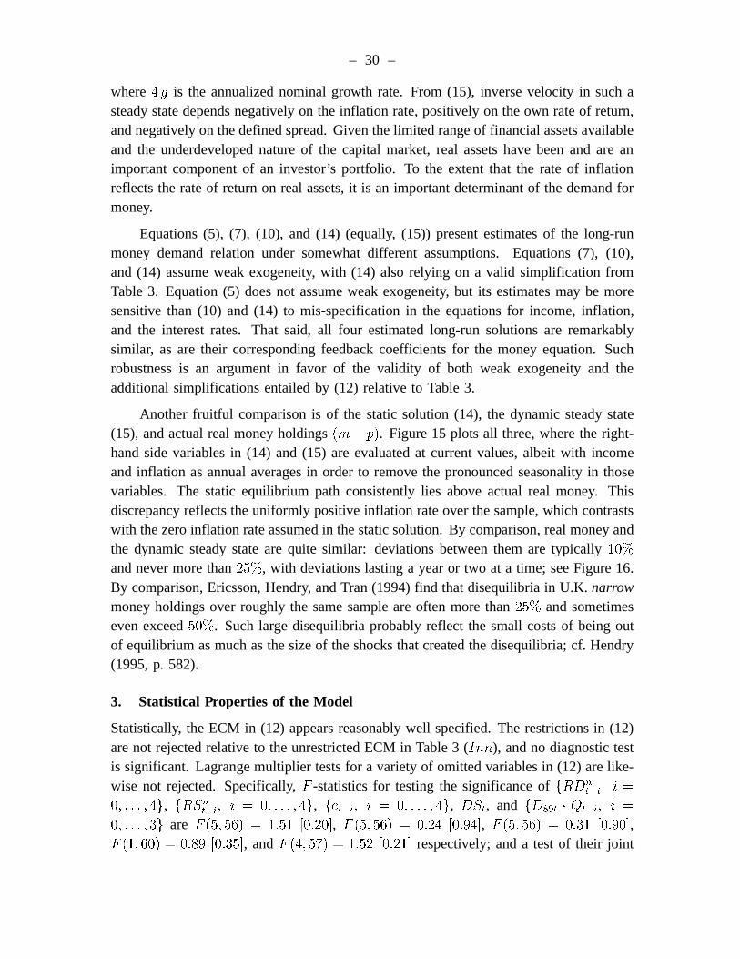
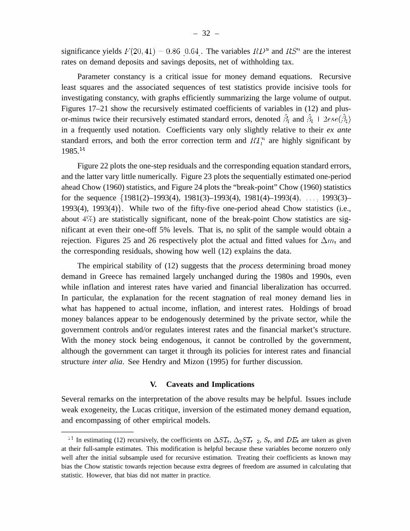
Parameter constancy is a critical issue for money demand equations. Recursiveleast squares and the associated sequences of test statistics provide incisive tools forinvestigating constancy, with graphs efficiently summarizing the large volume of output.Figures 17–21 show the recursively estimated coefficients of variables in (12) and plus-or-minus twice their recursively estimated standard errors, denoted^

tand ^

t§ 2ese( ^

t)

in a frequently used notation. Coefficients vary only slightly relative to theirex antestandard errors, and both the error correction term andRT n

tare highly significant by

1985.14

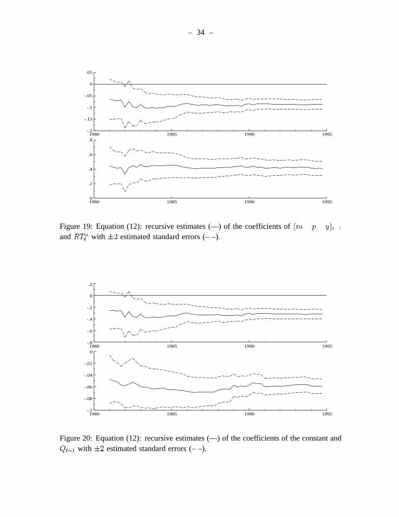
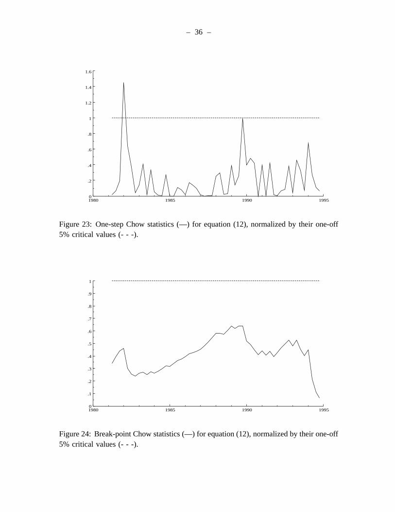
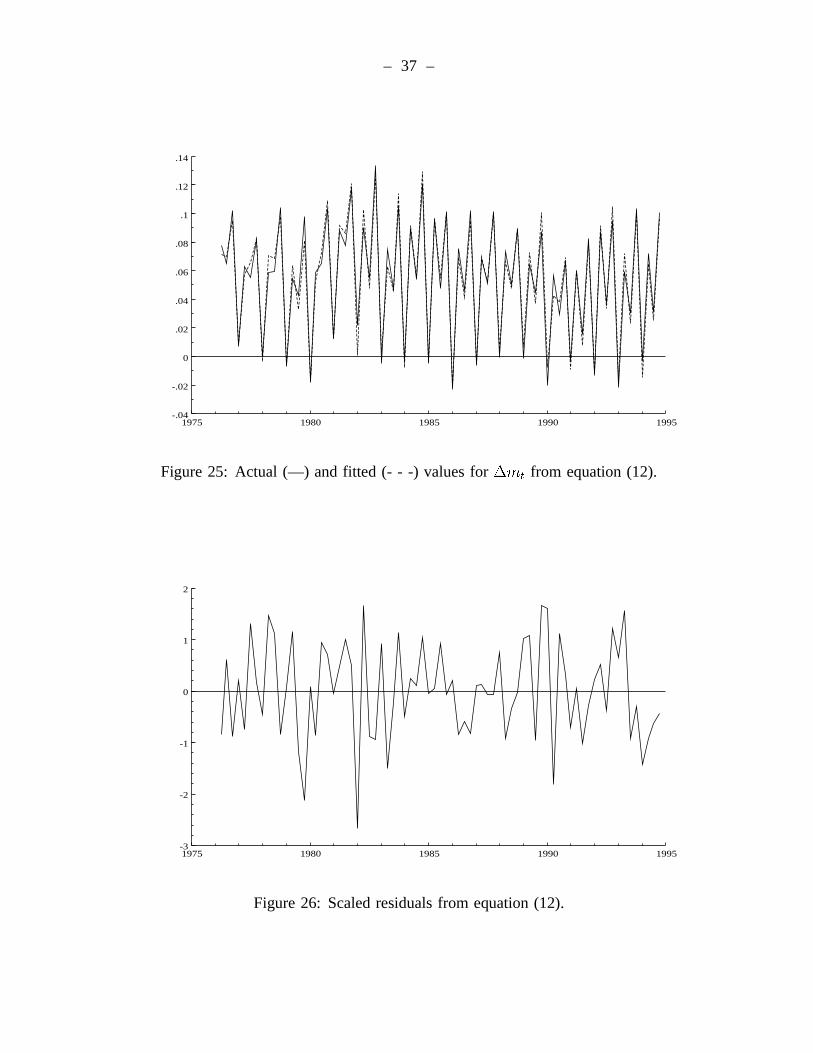
Figure 22 plots the one-step residuals and the corresponding equation standard errors,and the latter vary little numerically. Figure 23 plots the sequentially estimated one-periodahead Chow (1960) statistics, and Figure 24 plots the “break-point” Chow (1960) statisticsfor the sequencef1981(2)–1993(4), 1981(3)–1993(4), 1981(4)–1993(4); : : : ; 1993(3)–1993(4), 1993(4)g. While two of the fifty-five one-period ahead Chow statistics (i.e.,about4%) are statistically significant, none of the break-point Chow statistics are sig-nificant at even their one-off 5% levels. That is, no split of the sample would obtain arejection. Figures 25 and 26 respectively plot the actual and fitted values for¢m

tand

the corresponding residuals, showing how well (12) explains the data.

The empirical stability of (12) suggests that theprocessdetermining broad moneydemand in Greece has remained largely unchanged during the 1980s and 1990s, evenwhile inflation and interest rates have varied and financial liberalization has occurred.In particular, the explanation for the recent stagnation of real money demand lies inwhat has happened to actual income, inflation, and interest rates. Holdings of broadmoney balances appear to be endogenously determined by the private sector, while thegovernment controls and/or regulates interest rates and the financial market’s structure.With the money stock being endogenous, it cannot be controlled by the government,although the government can target it through its policies for interest rates and financialstructureinter alia. See Hendry and Mizon (1995) for further discussion.

V. Caveats and Implications

Several remarks on the interpretation of the above results may be helpful. Issues includeweak exogeneity, the Lucas critique, inversion of the estimated money demand equation,and encompassing of other empirical models.

14 In estimating (12) recursively, the coefficients on¢STt, ¢2STt¡2, St, andDEt are taken as givenat their full-sample estimates. This modification is helpful because these variables become nonzero onlywell after the initial subsample used for recursive estimation. Treating their coefficients as known maybias the Chow statistic towards rejection because extra degrees of freedom are assumed in calculating thatstatistic. However, that bias did not matter in practice.

– 33 –

1980 1985 1990 1995-.6

-.4

-.2

0

.2

.4

.6

1980 1985 1990 19950

.2

.4

.6

.8

1

1.2

Figure 17: Equation (12): recursive estimates (—) of the coefficients of¢mt¡1 and¢mt¡2 with §2 estimated standard errors (– –).

1980 1985 1990 1995-.8

-.6

-.4

-.2

0

.2

1980 1985 1990 1995-.2

0

.2

.4

.6

Figure 18: Equation (12): recursive estimates (—) of the coefficients of¢2pt and¢ytwith §2 estimated standard errors (– –).

– 34 –

1980 1985 1990 1995-.2

-.15

-.1

-.05

0

.05

1980 1985 1990 19950

.2

.4

.6

.8

Figure 19: Equation (12): recursive estimates (—) of the coefficients of(m¡ p¡ y)t¡1andRT n

twith §2 estimated standard errors (– –).

1980 1985 1990 1995-.8

-.6

-.4

-.2

0

.2

1980 1985 1990 1995-.1

-.08

-.06

-.04

-.02

0

Figure 20: Equation (12): recursive estimates (—) of the coefficients of the constant andQt¡1 with §2 estimated standard errors (– –).

– 35 –

1980 1985 1990 1995-.12

-.1

-.08

-.06

-.04

-.02

0

.02

.04

1980 1985 1990 1995-.08

-.06

-.04

-.02

0

.02

.04

.06

Figure 21: Equation (12): recursive estimates (—) of the coefficients ofQt¡2 andQt¡3

with §2 estimated standard errors (– –).

1980 1985 1990 1995-.02

-.015

-.01

-.005

0

.005

.01

.015

.02

Figure 22: One-step residuals (—) from equation (12), with0§ 2¾t (– –).

– 36 –

1980 1985 1990 19950

.2

.4

.6

.8

1

1.2

1.4

1.6

Figure 23: One-step Chow statistics (—) for equation (12), normalized by their one-off5% critical values (- - -).

1980 1985 1990 19950

.1

.2

.3

.4

.5

.6

.7

.8

.9

1

Figure 24: Break-point Chow statistics (—) for equation (12), normalized by their one-off5% critical values (- - -).

– 37 –

1975 1980 1985 1990 1995-.04

-.02

0

.02

.04

.06

.08

.1

.12

.14

Figure 25: Actual (—) and fitted (- - -) values for¢mt from equation (12).

1975 1980 1985 1990 1995-3

-2

-1

0

1

2

Figure 26: Scaled residuals from equation (12).

– 38 –

Section III established the weak exogeneity of output, inflation, and interest ratesfor the long-run parameters of the money demand relation. However,ex anteforecastingand counterfactual simulations for policy analysis are subject to several important caveats.First, ex anteforecasting requires specifying the paths for the “right-hand side” variables— output, inflation, and interest rates. Further, if multi-step ahead forecasts of moneydemand are constructed conditional on those future paths of the right-hand side variables,Granger noncausality fromm to p, y, RT n, ST , andSR is assumed, either implicitly orexplicitly. While weak exogeneity precludes explicit feedback in levels via the error cor-rection term, it does not exclude feedback through lagged growth rates. Empirically, onewould want to establish Granger noncausality before conducting conditional forecasting,or to develop models ofp, y, RT n, ST , andSR to permit jointly forecasting all variablesinvolved. On the latter approach, see Hendry and Mizon (1993) and Hendry and Doornik(1994) for U.K. money demand and Juselius (1993) for Danish money demand.

Counterfactual (policy) experiments require showing that the Lucas critique doesnot hold for the relevant class of interventions. That is, the money demand functionshould remain empirically constant, even when the marginal processes generating theother variables change. Formal tests for refuting the Lucas critique empirically appear inHendry (1988) and Engle and Hendry (1993), and they would be of interest to conductfor (12). The empirical constancy of (12) in the presence of financial deregulation ispartial evidence against the Lucas critique applying here.

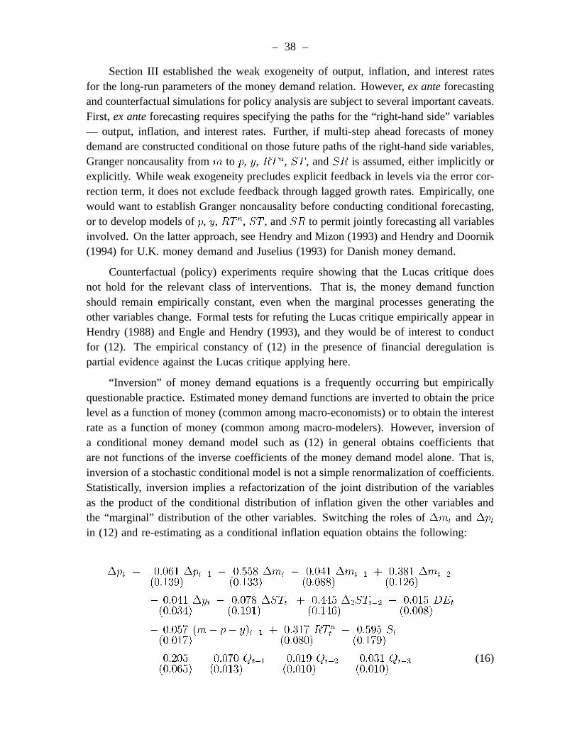
“Inversion” of money demand equations is a frequently occurring but empiricallyquestionable practice. Estimated money demand functions are inverted to obtain the pricelevel as a function of money (common among macro-economists) or to obtain the interestrate as a function of money (common among macro-modelers). However, inversion ofa conditional money demand model such as (12) in general obtains coefficients thatare not functions of the inverse coefficients of the money demand model alone. That is,inversion of a stochastic conditional model is not a simple renormalization of coefficients.Statistically, inversion implies a refactorization of the joint distribution of the variablesas the product of the conditional distribution of inflation given the other variables andthe “marginal” distribution of the other variables. Switching the roles of¢m

tand¢p

t

in (12) and re-estimating as a conditional inflation equation obtains the following:

¢pt= 0:061

(0:139)¢p

t¡1 ¡ 0:558(0:133)

¢mt¡ 0:041(0:088)

¢mt¡1 + 0:381

(0:126)¢m

t¡2

¡ 0:041(0:034)

¢yt¡ 0:078(0:191)

¢STt

+ 0:445(0:146)

¢2STt¡2 ¡ 0:015(0:008)

DEt

¡ 0:057(0:017)

(m¡ p¡ y)t¡1 + 0:317

(0:080)RT n

t¡ 0:595(0:179)

St

¡ 0:205(0:065)

¡ 0:070(0:013)

Qt¡1 ¡ 0:019

(0:010)Q

t¡2 ¡ 0:031(0:010)

Qt¡3 (16)

– 39 –

T = 75 [1976(2)¡ 1994(4)] R2 = 0:836 ¾ = 0:963% dw = 2:18

AR : F (5; 55) = 0:99 ARCH : F (4; 52) = 0:37

Normality : Â2(2) = 6:63¤ RESET : F (1; 59) = 1:14

Hetero : F (24; 35) = 0:69 :

The fit of (16) is not much better than that of themarginal equation for inflation inthe vector autoregression (¾ = 1:07%), and several coefficients in (16) do not makeeconomic sense. In particular, both the contemporaneous change in broad money and theerror correction term have negative coefficients, implying that increases in money and in“excess” holdings of money dampen inflation. Further, the money demand equation (12)is empirically constant, but its inversion (16) need not be so.

In principle, statistical comparison of models (encompassing) can help identify weak-nesses of the models being tested, and so indicate directions for their improvement.However, two practical difficulties prohibit calculating encompassing tests against otherresearchers’ models: no other empirical models currently exist that use the new measureof M3, and encompassing statistics for comparing models of different aggregates havenot yet been developed.

Models do exist for other measures of money. For the old measure of M3, Prodro-midis (1984) estimates static and partial adjustment models over 1966–1977, a samplethat is nearly non-overlapping with ours. Based on an EconLit bibliographic search,Prodromidis (1984) appears to be the only published empirical analysis of Greek M3demand. By contrast, many models of M1 have been published, with (e.g.) Psaradakis(1993) following a similar methodology to the one adopted above.

While currently no alternate models exist to encompass, some directions for improv-ing (12) are clear. In particular, for the returns on new assets and Treasury bills, theirmore gradual introduction in the model may better capture individuals’ actual responses.Learning-adjusted interest rates are one simple, intuitive formulation; see Hendry andEricsson (1991b) and Baba, Hendry, and Starr (1992).

VI. Concluding Remarks

The estimated conditional model of money demand in Greece is remarkably stable andotherwise well-specified over the period 1976–1994. The model’s empirical constancyholds in the face of large fluctuations in the inflation rate and a progressive — albeitslow — liberalization of the financial system. Even so, the fundamental changes currentlyunderway in the Greek financial system could alter the structure of the money demandfunction and, as a consequence, further complicate the conduct of monetary policy. Withrestrictions on external capital flows removed and financial deregulation in Greece ongo-ing, higher returns on assets inside M3 may increase the demand for money, while greateravailability of alternative assets (both domestic and foreign) may lower demand. For our

– 40 –

sample, the exchange rate did not significantly affect money demand once inflation wasincluded. With greater capital mobility, however, returns on foreign assets (and henceforeign interest rates and the exchange rate) are likely to influence money demand, as didthe increased availability of Treasury bills in the early 1990s. For money demand in theUnited States and the United Kingdom, Baba, Hendry, and Starr (1992) and Hendry andEricsson (1991b) show how the empirical adjustments to one financial innovation mayguide the specification of effects from future innovations. For Greece, the presence ofthe spreads in the estimated ECM suggests the potential empirical role of new alternativeassets in the demand for broad money.

– 41 –

Appendix I: Data Definitions

This appendix describes the data in greater detail. It lists the definitions used and givestheir units and sources. All data are quarterly and seasonally unadjusted, and the sampleperiod is from the first quarter of 1975 through the fourth quarter of 1994. The data werekindly provided to us by the Bank of Greece. To the extent possible, publicly availablesources are given for the series.

Monetary Aggregates and Their Components

Definition. The components of the broad money aggregate M3 (M ) are currency incirculation (CC), demand (or sight) deposits (DD), savings deposits (SD), time deposits(TD), bank bonds (BB), and repurchase agreements (repos) (REP ). Demand deposits,savings deposits, and time deposits are those held by individuals and private enterprises.Narrow money (M1) is currency in circulation plus demand deposits. In our sample,bank bonds were introduced in 1975(4), and repos in 1990(4).

Units. Billion (109) Drachmas. All figures are end-of-period balances.

Source. Monthly Statistical Bulletin, the Bank of Greece (Table 1 forCC andDD,Table 12 forSD andTD); andEconomic Bulletin, the Bank of Greece (Table III.1 forBB andREP ).

Treasury Bills

Definition. The stock of Treasury bills and one-year government bonds held by theprivate sector (TB).

Units. Billion (109) Drachmas, end-of-period balances.

Source. Economic Bulletin, the Bank of Greece (Table III.1).

Interest Rates

Definition. Interest rates on demand deposits (RD), savings deposits with commercialbanks (RS), time deposits at 12-month maturity for individuals and private enterprises(RT ), repurchase agreements (RR), and Treasury bills of 12-month maturity (RB). Eachrate is a weighted average of the various interest rates paid on the given financial instru-ment.

Units. Annual rate expressed as a fraction, calculated as the arithmetic average of monthly(average) rates.

Source. Bank of Greece (RD andRR); Monthly Statistical Bulletin, the Bank of Greece(Table 17 forRS andRT ); andEconomic Bulletin, the Bank of Greece (Table III.4 forRB).

– 42 –

Net Interest Rates

Definition. Interest rates, net of withholding tax, on demand deposits (RDn), savingsdeposits (RSn), time deposits (RT n), and repurchase agreements (RRn). The net interestrate is calculated as the gross interest rate times(1¡ ¿ ), where¿ is the withholding taxrate on interest payments. The government imposed a10 percent withholding tax onbank deposits in 1991(1). That tax was raised to12 percent in 1992(3) and to15 percentin 1992(4). In 1994(2), the government also imposed a withholding tax of15 percent onrepurchase agreements.

Units. Annual rate expressed as a fraction.

Source. Bank of Greece (¿ ).

Consumer Price Index

Definition. The general consumer price index (P ).

Units. 1988=100. The series was calculated as the arithmetic average of monthly values.To match the quarterly GDP figures, which have 1970 as their base year, the CPI serieswas then converted to base year 1970=100 by dividing by6:333=100.

Source. Monthly Statistical Bulletin, National Statistical Service of Greece (Table 75).

Real Output

Definition. Real gross domestic product (GDP) at factor cost (Y ). This is the onlyreal output variable for which a quarterly series was available. Until 1987, the seriescoincides with that reported by the National Statistical Service in itsMonthly StatisticalBulletin. From 1987 onwards, the series consists of figures adjusted by the Bank ofGreece to be consistent with the revised annual GDP figures for the new national accounts.The National Statistical Service’sMonthly Statistical Bulletinreports real GDP through1991(1), but based on the old national accounts. This latter series is denotedY old.

Units. Million Drachmas in 1970 prices.

Source. Monthly Statistical Bulletin, National Statistical Service of Greece (Table 97 forY andY old); and the Bank of Greece (forY from 1987 onwards).

The Nominal Effective Exchange Rate

Definition. Trade-weighted nominal effective exchange rate index (E). The index in-cludes the currencies of fifteen “competitor countries,” and the weights are based onnon-oil trade flows during 1981–1984.

Units. 1986=100.

Source. Economic Bulletin, the Bank of Greece (Table II.2).

– 43 –

Dummy Variables

Definition. The dummy variablesDE, DS, andD89 equal unity for the periods 1982(4)–1983(1), 1994(3)–1994(4), and 1989(1)–1994(4) respectively, and are zero otherwise.

Appendix II: Design of the Empirical ECM

This appendix discusses the steps taken to obtain the ECM in (12). The simplification to(12) has numerous motivations. Because of its parsimony and more orthogonal regressors,(12) is more easily interpreted than the unrestricted ADL or the vector autoregression.Also, the coefficients in (12) are more precisely estimated than those in the ADL and thevector autoregression, providing tighter inferences generally and higher potential powerfor tests of mis-specification.

The initial six-variable, fourth-order vector autoregression for the system cointegra-tion analysis was not simplified, either in terms of variables or in terms of lag length. Allsix variables appear to matter in the long run (Table 2 above). The Schwarz criterion doesfall monotonically in the sequential reduction from a fourth-order to a first-order vectorautoregression. However, many sets of variables at a given lag length are statisticallysignificant, so the lag length for the vector autoregression is kept at four.

Instead, simplification begins with weak exogeneity and then progresses throughlag reduction and variable transformation. Having tested for and found weak exogeneityfor real GDP, inflation, and the interest rates (Table 2), a fourth-order autoregressivedistributed lag for money is simplified to the ECM in (12). Table 3 above lists the esti-mates of the coefficients for the fourth-order ADL, where the ADL has been transformedinto an unrestricted ECM representation. The following variables do not appear eithernumerically or statistically significant in that representation.

(i) The lagspt¡1 andyt¡1 and the spreadSRt (all being long-run variables);(ii) All current and lagged values of¢RT n and¢SR; and(iii) The lags¢mt¡3, ¢yt¡1, ¢yt¡2, and¢yt¡3.

Three additional sets of reductions are considered:

(iv) The coefficients on¢pt and¢pt¡1 are equal and those on the remaining lags of¢pt are zero, in which case inflation enters as the single variable¢2pt;

(v) The coefficients on¢STt¡2 and¢STt¡3 are equal and the one on¢STt¡1 is zero,in which case this spread enters as¢STt and¢2STt¡2; and

(vi) The dummiesD89t ¢Qt¡i (i = 0; 1; 2; 3) andDSt have coefficients of zero.

Treated sequentially, these six restrictions obtain the following seven models.

– 44 –

Model 1: The unrestricted ECM in Table 3.Model 2: Model 1, imposing long-run price and income homogeneity and long-run

spread equality.Model 3: Model 2, excludingf¢RT n

t¡i;¢SRt¡i; i = 0; 1; 2; 3g.

Model 4: Model 3, excluding the lags¢mt¡3, ¢yt¡1, ¢yt¡2, and¢yt¡3.Model 5: Model 4, excluding¢pt¡1, ¢pt¡2, and¢pt¡3, once¢pt and¢pt¡1 have

been transformed to¢2pt and¢pt¡1.Model 6: Model 5, excluding¢STt¡1 and¢STt¡3, once¢STt¡2 and¢STt¡3 have

been transformed to¢2STt¡2 and¢STt¡3.Model 7: Model 6, excludingD89t ¢Qt¡i (i = 0; 1; 2; 3) andDSt.

So, for example, Model 2 is Model 1 plus reduction (i); Model 3 is Model 1 plusreductions (i)–(ii); and Model 3 is also Model 2 plus reduction (ii). Table 3 and equation(12) list the estimates for Models 1 and 7 and show how little the estimates change fromimposing the six reductions.

To facilitate formally assessing whether or not the sequence of reductions (i)–(vi) isvalid, and if not, where not, statistics associated with the implied reductions are calculatedfor all model pairs, and not only for adjacent models. Table II.1 reports this information,including the estimated equation standard error¾ and the Schwarz criterion for eachmodel, theF statistics for all model pairs, and the associated tail probability values. Theequation standard error is relatively constant across the entire simplification path, and theSchwarz criterion declines steadily throughout. Only one reduction (of excluding currentand lagged values of¢RT n and¢SR) is statistically significant at the 5% level; and it isonly barely so, and only when considered by itself and not in conjunction with additionalreductions. Other orderings of (i)–(vi) generate somewhat different statistics, but thoseresulting statistics are unlikely to be highly statistically significant because the reductionof (i)–(vi) as a whole appears valid, withF (25; 36) = 1:23 and ap-value of0:28.

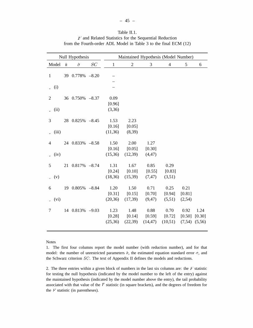
– 45 –

Table II.1.F and Related Statistics for the Sequential Reduction

from the Fourth-order ADL Model in Table 3 to the final ECM (12)

Null Hypothesis Maintained Hypothesis (Model Number)

Model k ¾ SC 1 2 3 4 5 6

1 39 0.778% –8.20 ––

# (i) –

2 36 0.750% –8.37 0.09[0.96]

# (ii) (3,36)

3 28 0.825% –8.45 1.53 2.23[0.16] [0.05]

# (iii) (11,36) (8,39)

4 24 0.833% –8.58 1.50 2.00 1.27[0.16] [0.05] [0.30]

# (iv) (15,36) (12,39) (4,47)

5 21 0.817% –8.74 1.31 1.67 0.85 0.29[0.24] [0.10] [0.55] [0.83]

# (v) (18,36) (15,39) (7,47) (3,51)

6 19 0.805% –8.84 1.20 1.50 0.71 0.25 0.21[0.31] [0.15] [0.70] [0.94] [0.81]

# (vi) (20,36) (17,39) (9,47) (5,51) (2,54)

7 14 0.813% –9.03 1.23 1.48 0.88 0.70 0.92 1.24[0.28] [0.14] [0.59] [0.72] [0.50] [0.30]

(25,36) (22,39) (14,47) (10,51) (7,54) (5,56)

Notes1. The first four columns report the model number (with reduction number), and for thatmodel: the number of unrestricted parametersk, the estimated equation standard error¾, andthe Schwarz criterionSC. The text of Appendix II defines the models and reductions.

2. The three entries within a given block of numbers in the last six columns are: theF statisticfor testing the null hypothesis (indicated by the model number to the left of the entry) againstthe maintained hypothesis (indicated by the model number above the entry), the tail probabilityassociated with that value of theF statistic (in square brackets), and the degrees of freedom fortheF statistic (in parentheses).

– 46 –

References

Akerlof, G. A. (1979) “Irving Fisher on His Head: The Consequences of ConstantThreshold-target Monitoring of Money Holdings,”Quarterly Journal of Economics,93, 2, 169–187.

Akerlof, G. A., and R. D. Milbourne (1980) “Irving Fisher on His Head II: The Conse-quences of the Timing of Payments for the Demand for Money,”Quarterly Journalof Economics, 95, 1, 145–157.

Alogoskoufis, G. (1995) “The Two Faces of Janus: Institutions, Policy Regimes andMacroeconomic Performance in Greece,”Economic Policy, 20, 147–192 (with dis-cussion).

Baba, Y., D. F. Hendry, and R. M. Starr (1992) “The Demand for M1 in the U.S.A.,1960–1988,”Review of Economic Studies, 59, 1, 25–61.

Banerjee, A., J. J. Dolado, J. W. Galbraith, and D. F. Hendry (1993)Co-integration, ErrorCorrection, and the Econometric Analysis of Non-stationary Data, Oxford, OxfordUniversity Press.

Banerjee, A., J. J. Dolado, D. F. Hendry, and G. W. Smith (1986) “Exploring Equilib-rium Relationships in Econometrics through Static Models: Some Monte CarloEvidence,”Oxford Bulletin of Economics and Statistics, 48, 3, 253–277.

Baumol, W. J. (1952) “The Transactions Demand for Cash: An Inventory TheoreticApproach,”Quarterly Journal of Economics, 66, 4, 545–556.

Boughton, J. M. (1991) “Money Demand in Five Major Industrialized Countries: Esti-mating and Interpreting Error Correction Models,” Chapter 4 in M. P. Taylor (ed.)Money and Financial Markets, Oxford, Basil Blackwell, 109–129.

Boughton, J. M. (1993) “The Demand for M1 in the United States: A Comment on Baba,Hendry, and Starr,”Economic Journal, 103, 420, 1154–1157.

Box, G. E. P., and D. A. Pierce (1970) “Distribution of Residual Autocorrelations inAutoregressive-integrated Moving Average Time Series Models,”Journal of theAmerican Statistical Association, 65, 332, 1509–1526.

de Brouwer, G., and N. R. Ericsson (1995) “Modelling Inflation in Australia,” Inter-national Finance Discussion Paper No. 530, Board of Governors of the FederalReserve System, Washington, D.C., November.

Chow, G. C. (1960) “Tests of Equality between Sets of Coefficients in Two Linear Re-gressions,”Econometrica, 28, 3, 591–605.

Dickey, D. A., and W. A. Fuller (1981) “Likelihood Ratio Statistics for AutoregressiveTime Series with a Unit Root,”Econometrica, 49, 4, 1057–1072.

Doornik, J. A., and H. Hansen (1994) “A Practical Test for Univariate and MultivariateNormality,” mimeo, Nuffield College, Oxford.

Doornik, J. A., and D. F. Hendry (1994)PcGive Professional 8.0: An Interactive Econo-metric Modelling System, London, International Thomson Publishing.

Durbin, J., and G. S. Watson (1950) “Testing for Serial Correlation in Least SquaresRegression. I,”Biometrika, 37, 3 and 4, 409–428.

– 47 –

Durbin, J., and G. S. Watson (1951) “Testing for Serial Correlation in Least SquaresRegression. II,”Biometrika, 38, 1 and 2, 159–178.

Engle, R. F. (1982) “Autoregressive Conditional Heteroscedasticity with Estimates of theVariance of United Kingdom Inflation,”Econometrica, 50, 4, 987–1007.

Engle, R. F., and C. W. J. Granger (1987) “Co-integration and Error Correction: Repre-sentation, Estimation, and Testing,”Econometrica, 55, 2, 251–276.

Engle, R. F., and D. F. Hendry (1993) “Testing Super Exogeneity and Invariance inRegression Models,”Journal of Econometrics, 56, 1/2, 119–139.

Ericsson, N. R. (1992) “Cointegration, Exogeneity, and Policy Analysis: An Overview,”Journal of Policy Modeling, 14, 3, 251–280.

Ericsson, N. R., J. Campos, and H.-A. Tran (1990) “PC-GIVE and David Hendry’sEconometric Methodology,”Revista de Econometria, 10, 1, 7–117.

Ericsson, N. R., D. F. Hendry, and H.-A. Tran (1994) “Cointegration, Seasonality, En-compassing, and the Demand for Money in the United Kingdom,” Chapter 7 inC. P. Hargreaves (ed.)Nonstationary Time Series Analysis and Cointegration, Ox-ford, Oxford University Press, 179–224.

Filippides, A. A., P. E. Kyriakopoulos, and D. M. Moschos (1995) “Bank of GreeceMonetary Policy Instruments,”Bank of Greece Economic Bulletin, 6, 55–63.

Friedman, M. (1956) “The Quantity Theory of Money — A Restatement,” Chapter 1 inM. Friedman (ed.)Studies in the Quantity Theory of Money, Chicago, Universityof Chicago Press, 3–21.

Godfrey, L. G. (1978) “Testing Against General Autoregressive and Moving Average ErrorModels when the Regressors Include Lagged Dependent Variables,”Econometrica,46, 6, 1293–1301.

Harvey, A. C. (1981)The Econometric Analysis of Time Series, Oxford, Philip Allan.

Hendry, D. F. (1988) “The Encompassing Implications of Feedback versus FeedforwardMechanisms in Econometrics,”Oxford Economic Papers, 40, 1, 132–149.

Hendry, D. F. (1995)Dynamic Econometrics, Oxford, Oxford University Press.

Hendry, D. F., and J. A. Doornik (1994) “Modelling Linear Dynamic Econometric Sys-tems,” Scottish Journal of Political Economy, 41, 1, 1–33.

Hendry, D. F., and N. R. Ericsson (1991a) “An Econometric Analysis of U.K. MoneyDemand inMonetary Trends in the United States and the United Kingdomby MiltonFriedman and Anna J. Schwartz,”American Economic Review, 81, 1, 8–38.

Hendry, D. F., and N. R. Ericsson (1991b) “Modeling the Demand for Narrow Moneyin the United Kingdom and the United States,”European Economic Review, 35, 4,833–886 (with discussion).

Hendry, D. F., and G. E. Mizon (1993) “Evaluating Dynamic Econometric Models byEncompassing the VAR,” Chapter 18 in P. C. B. Phillips (ed.)Models, Methods,and Applications of Econometrics: Essays in Honor of A. R. Bergstrom, Cambridge,Massachusetts, Basil Blackwell, 272–300.

Hendry, D. F., and G. E. Mizon (1995) “The Role of Exogeneity in Economic Policy

– 48 –

Analysis,” mimeo, Nuffield College, Oxford.

Hendry, D. F., and R. M. Starr (1993) “The Demand for M1 in the USA: A Reply toJames M. Boughton,”Economic Journal, 103, 420, 1158–1169.

Jarque, C. M., and A. K. Bera (1980) “Efficient Tests for Normality, Homoscedasticity andSerial Independence of Regression Residuals,”Economics Letters, 6, 3, 255–259.

Johansen, S. (1988) “Statistical Analysis of Cointegration Vectors,”Journal of EconomicDynamics and Control, 12, 2/3, 231–254.

Johansen, S. (1991) “Estimation and Hypothesis Testing of Cointegration Vectors inGaussian Vector Autoregressive Models,”Econometrica, 59, 6, 1551–1580.

Johansen, S. (1992a) “Cointegration in Partial Systems and the Efficiency of Single-equation Analysis,”Journal of Econometrics, 52, 3, 389–402.

Johansen, S. (1992b) “Testing Weak Exogeneity and the Order of Cointegration in UKMoney Demand Data,”Journal of Policy Modeling, 14, 3, 313–334.

Johansen, S. (1995)Likelihood-based Inference in Cointegrated Vector AutoregressiveModels, Oxford, Oxford University Press.

Johansen, S., and K. Juselius (1990) “Maximum Likelihood Estimation and Inference onCointegration — With Applications to the Demand for Money,”Oxford Bulletin ofEconomics and Statistics, 52, 2, 169–210.

Judd, J. P., and J. L. Scadding (1982) “The Search for a Stable Money Demand Function:A Survey of the Post-1973 Literature,”Journal of Economic Literature, 20, 3,993–1023.

Juselius, K. (1993) “VAR Modelling and Haavelmo’s Probability Approach to Macro-economic Modelling,”Empirical Economics, 18, 4, 595–622.

Kamin, S. B., and N. R. Ericsson (1993) “Dollarization in Argentina,” InternationalFinance Discussion Paper No. 460, Board of Governors of the Federal ReserveSystem, Washington, D.C., November.

Kremers, J. J. M., N. R. Ericsson, and J. J. Dolado (1992) “The Power of CointegrationTests,”Oxford Bulletin of Economics and Statistics, 54, 3, 325–348.

MacKinnon, J. G. (1991) “Critical Values for Cointegration Tests,” Chapter 13 in R. F. En-gle and C. W. J. Granger (eds.)Long-run Economic Relationships: Readings inCointegration, Oxford, Oxford University Press, 267–276.

MacKinnon, J. G., and H. White (1985) “Some Heteroskedasticity-consistent CovarianceMatrix Estimators with Improved Finite Sample Properties,”Journal of Economet-rics, 29, 3, 305–325.

Milbourne, R. (1983) “Optimal Money Holding Under Uncertainty,”International Eco-nomic Review, 24, 3, 685–698.

Miller, M. H., and D. Orr (1966) “A Model of the Demand for Money by Firms,”Quarterly Journal of Economics, 80, 3, 413–435.

Nicholls, D. F., and A. R. Pagan (1983) “Heteroscedasticity in Models with LaggedDependent Variables,”Econometrica, 51, 4, 1233–1242.

Osterwald-Lenum, M. (1992) “A Note with Quantiles of the Asymptotic Distribution of

– 49 –

the Maximum Likelihood Cointegration Rank Test Statistics,”Oxford Bulletin ofEconomics and Statistics, 54, 3, 461–472.

Prodromidis, K. P. (1984) “Determinants of Money Demand in Greece, 1966 I – 1977 IV,”Kredit und Kapital, 17, 3, 352–370.

Psaradakis, Z. (1993) “The Demand for Money in Greece: An Exercise in EconometricModelling with Cointegrated Variables,”Oxford Bulletin of Economics and Statis-tics, 55, 2, 215–236.

Ramsey, J. B. (1969) “Tests for Specification Errors in Classical Linear Least-squaresRegression Analysis,”Journal of the Royal Statistical Society, Series B, 31, 2,350–371.

Smith, G. W. (1986) “A Dynamic Baumol-Tobin Model of Money Demand,”Review ofEconomic Studies, 53, 3, 465–469.

Soumelis, G. (1995) “Greece: Reforming Financial Markets,”OECD Observer, 193,40–41.

Stock, J. H. (1994) “Unit Roots, Structural Breaks and Trends,” Chapter 46 in R. F. Engleand D. L. McFadden (eds.)Handbook of Econometrics, Amsterdam, North-Holland,Volume 4, 2739–2841.

Taylor, M. P. (1986) “From the General to the Specific: The Demand for M2 in ThreeEuropean Countries,”Empirical Economics, 11, 4, 243–261.

Tobin, J. (1956) “The Interest Elasticity of Transactions Demand for Cash,”Review ofEconomics and Statistics, 38, 3, 241–247.

Wallis, K. F. (1974) “Seasonal Adjustment and Relations between Variables,”Journal ofthe American Statistical Association, 69, 345, 18–31.

Watson, M. W. (1994) “Vector Autoregressions and Cointegration,” Chapter 47 inR. F. Engle and D. L. McFadden (eds.)Handbook of Econometrics, Amsterdam,North-Holland, Volume 4, 2843–2915.

White, H. (1980) “A Heteroskedasticity-consistent Covariance Matrix Estimator and aDirect Test for Heteroskedasticity,”Econometrica, 48, 4, 817–838.