www.ssoar.info

A Two-Factor Model for the Electricity ForwardMarketBöerger, Reik H.; Kiesel, Rüdiger; Schindlmayr, Gero

Postprint / PostprintZeitschriftenartikel / journal article

Zur Verfügung gestellt in Kooperation mit / provided in cooperation with:www.peerproject.eu

Empfohlene Zitierung / Suggested Citation:Böerger, Reik H. ; Kiesel, Rüdiger ; Schindlmayr, Gero: A Two-Factor Model for the Electricity Forward Market. In:Quantitative Finance 9 (2009), 3, pp. 279-287. DOI: http://dx.doi.org/10.1080/14697680802126530

Nutzungsbedingungen:Dieser Text wird unter dem "PEER Licence Agreement zurVerfügung" gestellt. Nähere Auskünfte zum PEER-Projekt findenSie hier: http://www.peerproject.eu Gewährt wird ein nichtexklusives, nicht übertragbares, persönliches und beschränktesRecht auf Nutzung dieses Dokuments. Dieses Dokumentist ausschließlich für den persönlichen, nicht-kommerziellenGebrauch bestimmt. Auf sämtlichen Kopien dieses Dokumentsmüssen alle Urheberrechtshinweise und sonstigen Hinweiseauf gesetzlichen Schutz beibehalten werden. Sie dürfen diesesDokument nicht in irgendeiner Weise abändern, noch dürfenSie dieses Dokument für öffentliche oder kommerzielle Zweckevervielfältigen, öffentlich ausstellen, aufführen, vertreiben oderanderweitig nutzen.Mit der Verwendung dieses Dokuments erkennen Sie dieNutzungsbedingungen an.

Terms of use:This document is made available under the "PEER LicenceAgreement ". For more Information regarding the PEER-projectsee: http://www.peerproject.eu This document is solely intendedfor your personal, non-commercial use.All of the copies ofthis documents must retain all copyright information and otherinformation regarding legal protection. You are not allowed to alterthis document in any way, to copy it for public or commercialpurposes, to exhibit the document in public, to perform, distributeor otherwise use the document in public.By using this particular document, you accept the above-statedconditions of use.

Diese Version ist zitierbar unter / This version is citable under:http://nbn-resolving.de/urn:nbn:de:0168-ssoar-221234

For Peer Review O

nly

A Two-Factor Model for the Electricity Forward Market

Journal: Quantitative Finance

Manuscript ID: RQUF-2006-0118.R2

Manuscript Category: Research Paper

Date Submitted by the Author:

31-Aug-2007

Complete List of Authors: Böerger, Reik; Ulm University, Financial Mathematics Kiesel, Rüdiger; Ulm University, Financial Mathematics Schindlmayr, Gero; EnBW Trading GmbH

Keywords: Energy Markets, Options, Term Structure, Model Calibration,

Commodity Markets, Implied Volatilities, Multi-factor Models

JEL Code: C51 - Model Construction and Estimation < C5 - Econometric Modeling < C - Mathematical and Quantitative Methods

Note: The following files were submitted by the author for peer review, but cannot be converted to PDF. You must view these files (e.g. movies) online.

RQUF-2006-0118.R2.zip

E-mail: quant@tandf.co.uk URL://http.manuscriptcentral.com/tandf/rquf

Quantitative Finance

For Peer Review O

nlyA Two-Factor Model for the Electricity Forward

Market

Rudiger Kiesel (Ulm University)Gero Schindlmayr (EnBW Trading GmbH)

Reik H. Borger (Ulm University)

August 30, 2007

Abstract

This paper provides a two-factor model for electricity futures, which captures the mainfeatures of the market and fits the term structure of volatility. The approach extendsthe one-factor-model of Clewlow and Strickland to a two-factor model and modifies it tomake it applicable to the electricity market. We will especially take care of the existenceof delivery periods in the underlying futures. Additionally, the model is calibrated tooptions on electricity futures and its performance for practical application is discussed.

Keywords: Energy derivatives, Futures, Option, Two-Factor Model, Volatility TermStructure

1 Introduction

Since the deregulation of electricity markets in the late 1990s, power can be traded onspot and futures markets at exchanges such as the Nordpool or the European EnergyExchange (EEX). Power exchanges established the trade of forwards and futures earlyon and by now large volumes are traded motivated by risk management and speculationpurposes.

Spot electricity is not a tradable asset which is due to the fact that it is non-storable.Thus, the spot trading and prices in electricity markets are not defined in the classicalsense. Similarly, electricity futures show contract specifications, that are different tomany other futures markets. In addition to the characterisation by a fixed delivery

1

Page 2 of 21

E-mail: quant@tandf.co.uk URL://http.manuscriptcentral.com/tandf/rquf

Quantitative Finance

123456789101112131415161718192021222324252627282930313233343536373839404142434445464748495051525354555657585960

For Peer Review O

nly

price per MWh and a total amount of energy to be delivered, power forward andfutures contracts specify a delivery period, which will directly influence the price of thecontract.

While much of the research in electricity markets focuses on the spot market (cp. Gemanand Eydeland [1999] for an introduction, Ventosa et al. [2005] for a survey of modellingapproaches, the monographs Eydeland and Wolyniec [2003], Geman [2005] for detailedoverviews, Weron [2006] for a discussion of time-series characteristics and distributionalproperties of electricity prices), only few results are available for electricity futures andoptions (on such futures).

For commodity futures modelling approaches can broadly be divided into two cate-gories. The first approach is to set up a spot-market model and derive the futures asexpected values under a pricing measure. The best-known representative is the two-factor model by Schwartz and Smith [2000], which uses two Brownian motions to modelshort-term variations and long-term dynamics of commodity spot prices. The authorsalso compute futures prices and prices for options on futures. However, electricity fu-tures are not explicitly modelled. In particular, the fact that electricity futures havea delivery over a certain period (instead of delivery at a certain point in time) is nottaken into account. Thus, the applicability to pricing options on electricity futures islimited.Several models more specific to electricity spot markets have extended the approachby Schwartz and Smith [2000] during the last few years. The typical model ingre-dients are a deterministic seasonality function plus some stochastic factors modelledby Levy processes. Typical representatives are Geman and Eydeland [1999], who useBrownian motions extended by stochastic volatilities and poisson jumps, Kellerhals[2001] and Culot et al. [2006], who use affine jump-diffusion processes, Cartea andFigueroa [2005], in which a mean-reverting jump-diffusion is suggested, Benth andSaltyte-Benth [2004], who apply Normal Inverse Gaussian processes, which is extendedto non-Gaussian Ornstein-Uhlenbeck processes in Benth et al. [2005]. Furthermore, aregime-switching factor process has been used in Huisman and Mahieu [2003]. All ofthese models are capable of capturing some of the features of the spot price dynamicswell and imply certain dynamics for futures prices, but these are usually quite involvedand difficult to work with. Especially, these models are not suitable when it comes tooption pricing in futures markets, since the evaluation of option pricing formulae is notstraightforward. In particular, none of the models has been calibrated to option pricedata.

The other line of research is to model futures markets directly, without consideringspot prices, using Heath-Jarrow-Morton-type of models (HJM). Here Chapter 5 of themonograph by Eydeland and Wolyniec [2003] provides a general summary of the mod-elling approaches for forward curves, but it does not apply a fully specified model toelectricity futures data. They rather point out that the modelling philosophy comingfrom the interest rate world can be applied to commodities markets in a refined ver-

2

Page 3 of 21

E-mail: quant@tandf.co.uk URL://http.manuscriptcentral.com/tandf/rquf

Quantitative Finance

123456789101112131415161718192021222324252627282930313233343536373839404142434445464748495051525354555657585960

For Peer Review O

nly

sion as well. The paper by Hinz et al. [2005] follows this line of research and providesarguments to justify this intuitive approach.

More direct approaches start with the well-known one-factor model by Clewlow andStrickland [1999] for general commodity futures. In principle, they can capture roughlyterm-structure features, which are present in many commodities markets, but theiremphasis is on the evaluation of options such as caps and floors, the derivation of spotdynamics within the model and building of trees, which are consistent with marketprices and allow for efficient pricing routines for derivatives on spot prices. Again, theydo not apply their model to the products of electricity markets and do not discussan efficient way of estimating parameters. A general discussion of HJM-type modelsin the context of power futures is given in Benth and Koekebakker [2005] (which canbe viewed as an extension of Koekebakker and Ollmar [2005]). They devote a largepart of their analysis to the relation of spot-, forward and swap-price dynamics andderive no-arbitrage conditions in power future markets and conduct a statistical studycomparing a one-factor model with several volatility specifications using data from NordPool market. Among other things, they conclude that a strong volatility term-structureis present in the market. The main empirical focus of both papers is to assess the fit ofthe proposed models to futures prices. While there are further studies using variantsof HJM-type model, e. g. Vehvilainen [2002], a successful application to the pricing ofoptions on electricity futures is still lacking.

One of the contributions of this paper is to address the issue of this pricing problem.In order to obtain an option pricing formula, we will follow the second line of research,that is, we will model the futures directly. We extend Clewlow and Strickland [1999]and Benth and Koekebakker [2005], in that we propose an explicit two-factor modeland fit it to option price data. Our main objective is to formulate a model and specify acertain volatility function, so that we are able to resemble the volatility term-structure.Thus, we will not use an Heath-Jarrow-Morton-type model, but rather set up a marketmodel in the spirit of LIBOR market models in the interest rate world. We regardthat as the second main contribution of the paper, since this approach enables us tomodel one-month futures as building blocks and derive prices of futures with differentdelivery period as portfolios of the building blocks. With this model we are not onlyable to price standardized options in the market but also to provide consistent pricesfor non-standard options such as options on seasonal contracts. In order to providepricing formulae for options on futures with a variety of delivery periods, we use anapproximation of the portfolio distribution and assess the quality of this approximation.We then provide option pricing formulae for all options in the market and use themarket-observed option prices to infer the model parameters. General two-factor modelspecification can be found in Schwartz and Smith [2000], Benth and Koekebakker [2005]and Lucia and Schwartz [2002] as well, but the parameter estimation uses time seriestechniques. By inferring risk-neutral parameters we avoid all complications related tothe specification of the market price of risk.

3

Page 4 of 21

E-mail: quant@tandf.co.uk URL://http.manuscriptcentral.com/tandf/rquf

Quantitative Finance

123456789101112131415161718192021222324252627282930313233343536373839404142434445464748495051525354555657585960

For Peer Review O

nly

We will show, that our model is robust, captures the term-structure of volatility and in-cludes the delivery over a period in futures and option prices. Thus, after the model hasbeen calibrated to plain-vanilla calls it can be used to price exotic options consistently(as soon as such options are traded).

The remainder of the paper is organised as follows. The following section describesthe EEX Futures and Option market to which our model is eventually calibrated.Section 3 develops our general modelling approach, while in section 4 a specific model isformulated. In section 5 we calibrate our model to market data and discuss the qualityof the fit. Section 6 concludes.

2 The EEX Futures and Options market

An electricity future is the obligation to buy or sell a specified amount of power ata predetermined delivery price during a fixed delivery period. The contract (i.e. thedelivery price) is set up such that initially no payment has to be made. While thedelivery price is fixed, the price which makes the contract have zero value will changeover time. This price is called futures price and is quoted at the exchanges.

The futures are standardized by the following characteristics: Volume, delivery periodand settlement.

The volume is fixed to a rate (energy amount per hour) of 1 Megawatt (MW). For adelivery period of e.g. September, this means a total of 1MW x 30days x 24h/day =720MWh. Quoted is the futures price per 1MWh. Smallest tick size is 0.01EUR perMWh.

The delivery periods are fixed to each of the 12 calendar months, the four quarters ofthe calendar year or the whole calendar year. When a year-contract comes to delivery,it is split up into the corresponding four quarters. A quarter, which is at delivery, issplit up into the corresponding three months and only the month at delivery will besettled either physically or financially.

Additional to these baseload contracts, there are peakload contracts, which deliverduring the day from 8am to 8pm Monday to Friday in the delivery period only. Theseare not considered in this paper.

At any fixed point in time, the next 6 months, 7 quarters and 6 years can be traded, butusually only the next 4 or 5 months, 5 quarters and 2 or 3 years show activity. Figure1 shows the available forward prices at September 14, 2005. (This represents a typicaltrading day and will be used throughout the text.) One might observe seasonalities inthe maturity variable T (not the time variable t), especially in the quarterly contracts:Futures during winter months show higher prices than comparable contracts during the

4

Page 5 of 21

E-mail: quant@tandf.co.uk URL://http.manuscriptcentral.com/tandf/rquf

Quantitative Finance

123456789101112131415161718192021222324252627282930313233343536373839404142434445464748495051525354555657585960

For Peer Review O

nly

Figure 1: Forward prices of futures with different maturities and delivery periods

summer

All options under consideration are European call options on baseload futures describedabove, which can be exercised only on the last day of trading, which coincides with theoptions maturity. The maturity is fixed according to a certain scheme, but usually itis on the 3rd Thursday of the month before delivery. The options are settled by theopening of a position in the corresponding future. The option prices are quoted in EURper MWh and the smallest tick size is 0.001EUR.

Available are options on the next five month-futures, six quarter-futures and threeyear-futures.

Especially the length of the delivery period and the time to maturity determine thevalue and statistical characteristics of the futures and options vitally. One can observe,that contracts with a long delivery period show less volatile prices than those withshort delivery. This is called term structure of volatility and is present in most powerfutures markets. The term structure has to be modelled accurately in order to be ableto price options on futures. Figure 2 gives an example of such a term structure forfutures traded at the EEX. The figure shows the volatility of futures contracts, which isobtained by inverting the Black-formula that evaluates options on these futures. Froman economic point of view it is clear, that futures with long delivery period are lessvolatile than those with short delivery, since the arrival of news such as temperature,outages, oil price shocks etc. influence usually only certain months of the year and

5

Page 6 of 21

E-mail: quant@tandf.co.uk URL://http.manuscriptcentral.com/tandf/rquf

Quantitative Finance

123456789101112131415161718192021222324252627282930313233343536373839404142434445464748495051525354555657585960

For Peer Review O

nly

Figure 2: Option-implied volatilities of futures with different delivery periods and de-livery starting dates

will average out in the long run with opposite news for other months. Only if allone-months contracts move in the same direction, the corresponding year contract willmove as well. Furthermore, the arrival of news will accelerate when a contract comesto delivery, since temperature forecasts, outages and other specifics about the deliveryperiod become more and more precise. Thus, the volatility increases.

We will show, that our modelling approach using one-month contracts as buildingblocks, will enable us to capture the term-structure of volatility and the influence ofthe period of delivery.

3 Description of the Model and Option Pricing

3.1 General Model Formulation

In energy markets we observe futures with different delivery periods. In the following,energy futures with 1-month delivery are the building blocks of our model. Note,that futures with other delivery period are derivatives now, i.e. a future with deliveryof a year is a portfolio of 12 appropriate month-futures. For a full treatment of no-arbitrage conditions and the relations between electricity futures compare Benth and

6

Page 7 of 21

E-mail: quant@tandf.co.uk URL://http.manuscriptcentral.com/tandf/rquf

Quantitative Finance

123456789101112131415161718192021222324252627282930313233343536373839404142434445464748495051525354555657585960

For Peer Review O

nly

Koekebakker [2005].

Let F (t, T ) denote the time t forward price of 1MWh electricity to be delivered con-stantly over a 1-month-period starting at T . Then, assuming a deterministic and flatrate of interest r, the time t value of this futures contract with delivery price D is givenby

V future(t, T ) = e−r(T−t) (F (t, T )−D) .

D is the price for 1MWh electricity delivered constantly during the 1-month-periodagreed upon at the time of signing the forward contract. Assuming the existence ofa risk-neutral measure, discounted value processes have to be martingales under thismeasure, which in this case is equivalent to forward prices being martingales.

Thus, in the spirit of LIBOR market models, we model the observable forward pricesdirectly under a risk-neutral measure as martingales via the stochastic differential equa-tion

dF (t, T ) = σ(t, T )F (t, T )dW (t),

where σ(t, T ) is an adapted d-dimensional deterministic function and W (t) a d-dimensionalBrownian motion. The initial value of this SDE is given by the condition to fit the ini-tial forward curve observed at the market. This takes care of the seasonality in thematurity variable T .

The solution of the SDE is given by

F (t, T ) = F (0, T ) exp

(∫ t

0

σ(s, T )dW (s)− 1

2

∫ t

0

||σ(s, T )||2ds

)

where || · || is the standard Euclidean norm on Rd.

3.2 Option Pricing

A European call option on F (t, T ) with maturity T0 and strike K can be easily evaluatedby the Black-formula

V option(t) = e−r(T0−t) (F (0, T )N (d1)−KN (d2)) , (1)

where N denotes the normal distribution and

d1 =log F (0,T )

K+ 1

2Var(log F (T0, T ))√

Var(log F (T0, T ))

d2 = d1 −√

Var(log F (T0, T ))

We now use month-futures to describe futures with longer delivery period. In particular,options on year-futures are the most heavily traded products in the option market. To

7

Page 8 of 21

E-mail: quant@tandf.co.uk URL://http.manuscriptcentral.com/tandf/rquf

Quantitative Finance

123456789101112131415161718192021222324252627282930313233343536373839404142434445464748495051525354555657585960

For Peer Review O

nly

price such options, year-futures (i. e. futures with delivery period 1 year) are a portfolioof the building blocks, the month-futures. Thus, the pricing of an option on such aportfolio is not straightforward and a closed form formula is not known in general. Theissue is closely related to the pricing of swaptions in the context of LIBOR marketmodels and is discussed in Brigo and Mercurio [2001].

The value of a portfolio of month-futures (e. g. a year-future) with delivery starts atTi, i = 1, . . . n normalized to the delivery of 1 MWh and delivery price D is given by

V portfolio(t, T1, . . . , Tn) =1

n

n∑i=1

e−r(Ti−t) (F (t, Ti)−D) .

In the context of interest rate swaps, the value of a swap is expressed in terms of aswap rate Y , which is here:

V portfolio(t, T1, . . . , Tn) =1

n

n∑i=1

e−r(Ti−t) (YT1,...,Tn(t)−D) ,

where

YT1,...,Tn(t) =

∑ni=1 e−r(Ti−t)F (t, Ti)∑n

i=1 e−r(Ti−t).

In case the portfolio represents a 1-year-future, the swap rate is the forward price ofthe 1-year-future, which can be also observed in the market.

Evaluating an option on this 1-year-forward price (i. e. on the swap par rate) posesthe problem of computing the expectation in

e−rT0E[(Y (T0)−K)+]

,

where the distribution of Y as a sum of lognormals is unknown. We use an approxima-tion as suggested by e. g. Brigo and Mercurio [2001], which assumes Y to be lognormal.Formally, we can approximate Y by a random variable Y , which is lognormal and co-incides with Y in mean and variance. Then,

log Y ∼ N (m, s)

with s2 depending on the choice of the volatility functions σ(t, Ti).

Using this approximation, it is possible to apply a Black-option formula again to obtainthe option value as

V option = e−rT0E[(Y (T0)−K)+]

≈ e−rT0E[(

Y (T0)−K)+

]= e−rT0 (Y (0)N (d1)−KN (d2)) (2)

8

Page 9 of 21

E-mail: quant@tandf.co.uk URL://http.manuscriptcentral.com/tandf/rquf

Quantitative Finance

123456789101112131415161718192021222324252627282930313233343536373839404142434445464748495051525354555657585960

For Peer Review O

nly

with

d1 =log Y (0)

K+ 1

2s2

sd2 = d1 − s

The approximation has been proposed by Levy [1992] in the context of pricing optionson arithmetic averages of currency rates. This density approximation competes mainlywith Monte Carlo methods and modifications of the price of the corresponding geometricaverage option. The advantage of the approximation to Monte Carlo simulation isclearly the difference in speed in which an option evaluation can be carried out, whichbecomes even more dramatic when turning the focus to calibration. The main drawbackof the manipulation of arithmetic average options is that it yields pricing formulae,which do not satisfy the put-call parity in general.

An empirical discussion of the goodness of the approximation in the context of cur-rency exchange rates is also provided by Levy [1992]. A comparison of second momentsleads to errors that are usually much smaller than 1%, especially when the underlying’svolatility is below 50%. While skewness is present in the true but not in the approx-imated distribution, kurtosis is matched very well. Another study emphasizing theapplicability of this approximation in interest rates markets can be found in Brigo andLiinev [2005]. A simulation study done by us in the case of electricity futures shows,that the difference between the true distribution of the sum and the approximatingdistribution is very small and becomes negligible considering other uncertainties in theapplication such as quality of market quotes.

4 The Special Case of a Two-Factor-Model

As motivated in the introductory part, a special choice of the volatility function isneeded to resemble market observations of the term structure of volatility in the futurescontracts. In this section we will use a two-factor model given by the SDE

dF (t, T )

F (t, T )= e−κ(T−t)σ1 dW 1

t + σ2 dW 2t , (3)

for a fixed T . The Brownian motions are assumed to be uncorrelated.

This is a special case of the general setup in the previous section with

σ(t, T ) =(e−κ(T−t)σ1, σ2

)and W (t) a 2-dimensional Brownian motion.

9

Page 10 of 21

E-mail: quant@tandf.co.uk URL://http.manuscriptcentral.com/tandf/rquf

Quantitative Finance

123456789101112131415161718192021222324252627282930313233343536373839404142434445464748495051525354555657585960

For Peer Review O

nly

For ease of notation assume in the following that today’s time t = 0.

This choice of volatility is motivated by the shape of the term structure of volatility (cp.Figure 2). The strong decrease will be modelled by the first factor with an exponentiallydecaying volatility function. Thus, futures maturing later will have a lower volatilitythan futures maturing soon. Finally, as T −t becomes very large, the volatility assignedto the contract by this factor will be close to zero. As this is not the case in practice,we introduce a second factor, which will keep the volatility away from zero.

Another way of viewing the two factors comes from the economic interpretation: Thefirst factor captures the increased trading activity as knowledge about weather, unex-pected outages etc. becomes available. The second factor models a long-term uncer-tainty, that is common to all products in the market. This uncertainty can be explainedby technological advances, political changes, price developments in other commoditymarkets and many more.

Within this two-factor model, the variance of the logarithm of the future contract atsome future time T0 can be computed easily (see the Appendix):

Var(log F (T0, T )) =σ2

1

2κ(e−2κ(T−T0) − e−2κT ) + σ2

2T0 (4)

This quantity has to be used to price an option on month-futures with maturity T0

with the option formula (1).

In the case of options on quarter- or year-futures, it is necessary to compute the quantitys2 of the lognormal approximation in equation (2). The derivation of s2 in this two-factor model can be found in Appendix and is given by

exp(s2) =

∑i,j e−r(Ti+Tj)F (0, Ti)F (0, Tj) · exp (Covij)

(∑

e−r·TiF (0, Ti))2 (5)

Covij = Cov(log F (T0, Ti), log F (T0, Tj))

= e−κ(Ti+Tj−2T0) σ21

2κ(1− e−2κT0) + σ2

2T0

5 Fitting the model

5.1 Calibration procedure

In order to calibrate the two-factor model to market data, we need to estimate theparameters φ = (σ1, σ2, κ) such that the model fits the market behaviour. Since wehave modelled under a risk-neutral measure, we need to find risk-neutral parameters,which can be observed using option-implied parameters.

10

Page 11 of 21

E-mail: quant@tandf.co.uk URL://http.manuscriptcentral.com/tandf/rquf

Quantitative Finance

123456789101112131415161718192021222324252627282930313233343536373839404142434445464748495051525354555657585960

For Peer Review O

nly

Given the market price of a futures-option (month-, quarter- or year-futures), we canobserve its implied variance Var(log(F (T0, T )) for month-future or s2 for quarter- oryear-futures.

Furthermore, we can compute the corresponding model implied quantities, which de-pend on the choice of the parameter set φ = (σ1, σ2, κ) as described in the previoussection. We will estimate the model parameters such that the squared difference ofmarket and model implied quantities is minimal, i. e.∑

i

(Varmarket(log YT1i

,...Tni(T0i

))− Varφmodel(log YT1i

,...,Tni(T0i

)))2

→ argminφ

, (6)

where i represents an option with maturity T0iand delivery covering the months

T1i, . . . , Tni

. Depending on the delivery period, which of course may be longer thanone month, the model variance is either the true model implied variance according toequation (4) or the approximated variance according to equation (5). The minimum istaken over all admissible choices of φ = (σ1, σ2, κ), that means σ1,2, κ > 0.

Since our model is not capable of capturing volatility smiles, which can be observed inoption prices very often, we will use at-the-money options only.

The minimization can be done with standard programming languages and their imple-mented optimizers. The objective function (6) is given to the optimizer, which has tocompute the model implied variances of all options for different parameters. The worstcase (the computation of the variance of a year-contract) involves the evaluation of allcovariances Covij between the underlying month-futures in equation (5), which is a 12by 12 matrix, thus computationally not too expensive. As there are usually not morethan 15 at-the-money options available (e. g. at the EEX), the optimization can bedone within a few minutes.

Additionally, it is possible to use the gradient of the objective function for the optimiza-tion. The gradient can be computed explicitly, which makes the numerical evaluationof the gradient in the optimizers unnecessary. Usually, there is a smaller number offunction calls necessary to reach the optimal point within a given accuracy using thegradient than using a numerical approximation. But, the explicit calculation again in-volves matrices up to size 12 by 12. We found, that the time saved by less function callsis eaten up by the increased complexity of the problem. Both methods end up withabout the same optimization time, though the gradient method finds minima, whichusually give slightly smaller optimal values than methods without gradient.

5.2 Calibration to Option Prices

In the following we will apply the two-factor model introduced in Section 4 to theGerman market, i. e. we will calibrate it to EEX prices. We repeated the procedure

11

Page 12 of 21

E-mail: quant@tandf.co.uk URL://http.manuscriptcentral.com/tandf/rquf

Quantitative Finance

123456789101112131415161718192021222324252627282930313233343536373839404142434445464748495051525354555657585960

For Peer Review O

nly

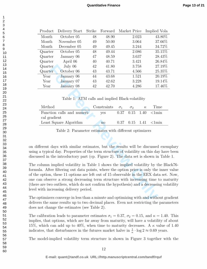
Product Delivery Start Strike Forward Market Price Implied Vola

Month October 05 48 48.90 2.023 43.80%Month November 05 49 50.00 3.064 37.66%Month December 05 49 49.45 3.244 34.72%Quarter October 05 48 49.44 2.086 35.15%Quarter January 06 47 48.59 3.637 28.43%Quarter April 06 40 40.71 3.421 26.84%Quarter July 06 42 41.80 3.758 27.19%Quarter October 06 43 43.71 4.566 25.35%

Year January 06 44 43.68 1.521 20.19%Year January 07 43 42.62 3.228 19.14%Year January 08 42 42.70 4.286 17.46%

Table 1: ATM calls and implied Black-volatility

Method Constraints σ1 σ2 κ Time

Function calls and numeri-cal gradient

yes 0.37 0.15 1.40 <1min

Least Square Algorithm no 0.37 0.15 1.41 <1min

Table 2: Parameter estimates with different optimizers

on different days with similar estimates, but the results will be discussed exemplaryusing a typical day. Properties of the term structure of volatility on this day have beendiscussed in the introductory part (cp. Figure 2). The data set is shown in Table 1.

The column implied volatility in Table 1 shows the implied volatility by the Black76-formula. After filtering out data points, where the option price is only the inner valueof the option, these 11 options are left out of 15 observable in the EEX data set. Now,one can observe a strong decreasing term structure with increasing time to maturity(there are two outliers, which do not confirm the hypothesis) and a decreasing volatilitylevel with increasing delivery period.

The optimizers converge in less than a minute and optimizing with and without gradientdelivers the same results up to two decimal places. Even not restricting the parametersdoes not change the estimates (see Table 2).

The calibration leads to parameter estimates σ1 = 0.37, σ2 = 0.15, and κ = 1.40. Thisimplies, that options, which are far away from maturity, will have a volatility of about15%, which can add up to 40%, when time to maturity decreases. A κ value of 1.40indicates, that disturbances in the futures market halve in 1

κ· log 2 ≈ 0.69 years.

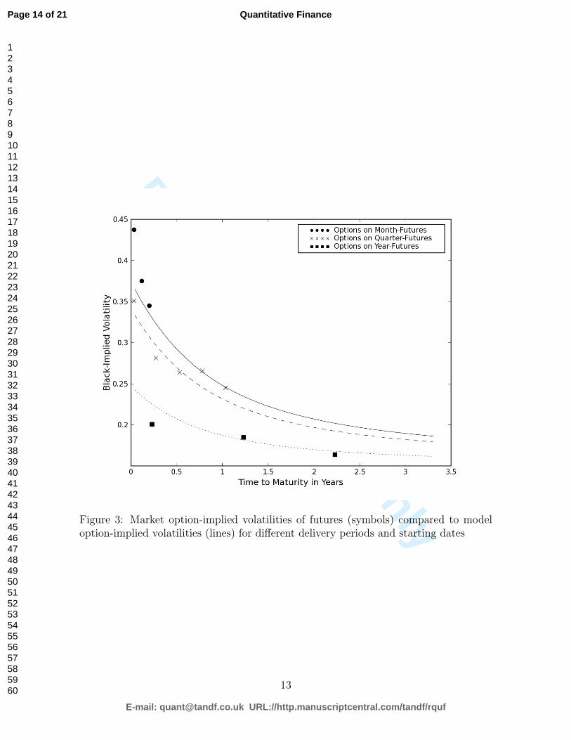
The model-implied volatility term structure is shown in Figure 3 together with the

12

Page 13 of 21

E-mail: quant@tandf.co.uk URL://http.manuscriptcentral.com/tandf/rquf

Quantitative Finance

123456789101112131415161718192021222324252627282930313233343536373839404142434445464748495051525354555657585960

For Peer Review O

nlyFigure 3: Market option-implied volatilities of futures (symbols) compared to modeloption-implied volatilities (lines) for different delivery periods and starting dates

13

Page 14 of 21

E-mail: quant@tandf.co.uk URL://http.manuscriptcentral.com/tandf/rquf

Quantitative Finance

123456789101112131415161718192021222324252627282930313233343536373839404142434445464748495051525354555657585960

For Peer Review O

nly

Delivery Start MarketPrice

ModelPrice

MarketVolatility

ModelVolatility

M-October 05 2.023 1.844 43.80% 38.52%M-November 05 3.064 3.000 37.66% 36.70%M-December 05 3.244 3.279 34.72% 35.13%Q-October 05 2.086 2.089 35.15% 35.25%Q-January 06 3.637 3.865 28.43% 30.82%Q-April 05 3.421 3.539 26.84% 27.88%Q-July 06 3.758 3.520 27.19% 25.51%

Q-October 06 4.566 4.315 25.35% 23.83%Y-January 06 1.521 1.746 20.19% 22.92%Y-January 07 3.228 3.074 19.14% 18.28%Y-January 08 4.286 4.131 17.62% 16.93%

Table 3: Comparison between market and model quantities

observed market values. One can see, that, qualitatively, most of the desired propertiesare described by the model. Futures with a long delivery period show a lower levelof volatility compared to those with short delivery. The volatility term structure isdecreasing as the time to maturity increases, but it does not go down to zero. Yet,quantitatively, there are some drawbacks. Especially the month-futures show a volatilityterm structure, that has a much steeper slope than the model implies. Also, the level ofvolatility is mostly higher than observed in the market, which seems to be the trade-offbetween fitting all options well at the short end and at the long end. Yet, the modelimplies reasonable values for all contracts. Absolute values in terms of volatilities andoption prices can be taken from Table 3.

5.3 Parameter Stability

In the following we discuss parameter stability. Common procedures are to recalibratethe model frequently on several days and analyze the stability of parameters over time,for different strikes and infer confidence intervals for the parameters. All this requires aliquid options market. This is still not the case for the EEX electricity market. Almostsimultaneously to the introduction of option trading, electricity prices increased sharply.This left the market with deep in-the-money call options, which are not suitable fortesting the model introduced above. More recently, decreasing prices at the EEX insome products lead to many options which are deep out-of-the-money. Only duringthe last couple of months, it seems as if the market has stabilized and there are quotesfor (almost) ATM options and a preliminary analysis of parameter stability is possible.Yet, we want to point out that the longer we go back into recent history, options on

14

Page 15 of 21

E-mail: quant@tandf.co.uk URL://http.manuscriptcentral.com/tandf/rquf

Quantitative Finance

123456789101112131415161718192021222324252627282930313233343536373839404142434445464748495051525354555657585960

For Peer Review O

nly

month-futures are more and more out-of-the-money.

We estimated parameters daily using the valid forward curves and market prices ofoptions that are closest to at-the-money. We use a history of 52 trading days from June1 to August 13. Figure 4 shows the evolution of parameters over time.

We can clearly identify very stable estimates for the parameter σ2, which reflects thevolatility at the long end of the term-structure. It is mainly determined by optionson year-futures, which are available at many strike levels, in particular we observeevery day at-the-money option prices. The stability of this estimate is in line with theintuition that long-delivery futures are less sensitive to market changes which shouldresult in low volatility and a low variability of the volatility estimates.

σ1 and κ describe the volatility level at the short end of the term-structure and thespeed of decrease of the term-structure, respectively. The estimate of σ1 fluctuates morethan that of σ2 but changes are not substantial. The changes can be explained by thesensitivity of option prices to the changes in the underlying. Especially the one-monthoptions are rarely exactly at-the-money, the change in one underlying can change thevolatility term-structure drastically, in particular when considering that the volatilitysmile can be quite steep in electricity markets. This forces the estimate σ1 to react tothe changed condition.

Besides the high volatility of the month-futures, the imperfectness of the at-the-money-assumptions contributes to the changes of the estimate for κ. Futures prices at the shortend of the curve have moved constantly to the smallest strike level of the correspondingoptions from below. In other words, options, that have been out-of-the-money at thebeginning of the period, are less so at the end. These options have an increased volatilitycompared to ATM options, which leads to a bigger gap between the short end of theterm-structure (mostly options on one-month futures) and the long end of the term-structure (options on year-futures). A large value of κ is required to induce a steepterm-structure within in the model. Since the steepness in the market is decreasingover time, κ is decreasing, too.

Considering the correlation of parameter estimates, we find support for the argumenta-tion above (cp. Table 4). The correlation between κ and σ1 of about 0.64 is substantial,which coincides with the argument that both are driven by the moneyness of the short-end volatilities.

Computing standard deviations from the estimates yields Table 4, which allows tocompute asymptotic confidence intervals for each parameter. While standard deviationsare rather low for σ1 and σ2 as one might expect from Figure 4, it is much higher for κ.Yet, constructing standard confidence intervals for each parameter leads to a decisiverejection of the hypothesis of zero values for any of the parameters at a 99% level ofconfidence.

15

Page 16 of 21

E-mail: quant@tandf.co.uk URL://http.manuscriptcentral.com/tandf/rquf

Quantitative Finance

123456789101112131415161718192021222324252627282930313233343536373839404142434445464748495051525354555657585960

For Peer Review O

nly

Figure 4: Change in parameter estimates over a 10 week period

Correlation σ1 σ2 κ Mean Std

σ1 1.00 0.16 0.63 0.57 0.052σ2 1.00 -0.41 0.16 0.012κ 1.00 1.96 0.536

Table 4: Correlation, mean and standard deviation of parameter estimates

16

Page 17 of 21

E-mail: quant@tandf.co.uk URL://http.manuscriptcentral.com/tandf/rquf

Quantitative Finance

123456789101112131415161718192021222324252627282930313233343536373839404142434445464748495051525354555657585960

For Peer Review O

nly

6 Conclusion

We have presented a two-factor-model for the electricity futures market. It is embeddedin a bigger class of market models, which are similar to the very popular market modelsin the interest rate markets. We have developed pricing formulae for relevant productsin the market and shown a procedure to fit the market data.

The main results of the work are, firstly, a very good overall fit of the model to optionimplied volatilities, especially for options on futures with long delivery period and nottoo close to maturity. Secondly, an excellent incorporation of the length of deliveryperiod into the option pricing. Thirdly, we showed that the model and the calibrationprocedure work fast and reliable and are ready to use for day-to-day application.

Nevertheless, we have to mention an unsatisfactory fit at the very short end of thevolatility term-structure for one-month futures. This might be due to the assumptionof lognormal returns. While this assumption is acceptable for some futures contracts inthe electricity market for practical applications, it breaks down as the delivery periodis short (i. e. one month) and the contract is close to maturity (i. e. last two monthsof trading), in other words, the more the futures contract approximates the spot price.Possible solutions to this shortcoming might be the inclusion of jumps into the modelor another specification of Levy-process driving the background noise. Additionally,this can broaden the data basis for fitting purposes, in that we can price and use otherthan at-the-money options only.

17

Page 18 of 21

E-mail: quant@tandf.co.uk URL://http.manuscriptcentral.com/tandf/rquf

Quantitative Finance

123456789101112131415161718192021222324252627282930313233343536373839404142434445464748495051525354555657585960

For Peer Review O

nly

7 Appendix

All following results will be derived under the assumption of correlated Brownian mo-tions, i. e. dW

(1)t dW

(2)t = ρdt (in contrast to the independence assumption in the

article). The results of the article will be obtained by setting ρ = 0.

Derivation of the Variance of a Month-Futures ContractWe will derive equation (4), i. e. Var(log F (T0, T ). The SDE describing the futuresdynamics in equation (3) can be solved by

F (t, T ) = F (0, T ) exp

{−1

2

∫ t

0

σ2(s, T )ds +

∫ t

0

e−κ(T−s)σ1dW (1)s +

∫ t

0

σ2dW (2)s

}σ2(s, t) = σ2

1e−2κ(t−s) + 2ρσ1σ2e

−κ(t−s) + σ22.

Now

Var(log F (T0, T )) =σ2

1

2κ(e−2κ(T−T0) − e−2κT ) + σ2

2T0 + 2ρσ1σ2

κ(e−κ(T−T0) − e−κT )

Derivation of the Variance of Quarter- and Year-Futures ContractsWe will derive equation (5), i. e. s2 at time T0. We have

E(Y ) = E(Y ), Var(Y ) = Var(Y ), log Y ∼ N (m, s2).

Moments of normal and lognormal distributions are related via

E(Y ) = exp(m +1

2s2), Var(Y ) = exp(2m + 2s2)− exp(2m + s2)

Solving this system, we get exp(s2) = Var(Y )

(E(Y ))2+ 1 = E(Y 2)

E(Y )2. It can be seen easily that

E(FT0,Ti) = F0,Ti

, E(YT1,...Tn(T0)) =

∑e−r(Ti−T0)F0,Ti∑

e−r(Ti−T0)

Further

E(YT1,...Tn(T0)2) =

1

(∑

e−r(Ti−T0))2 · ...∑

i,j

e−r(Ti+Tj−2T0)F0,TiF0,Tj

· exp Covij

Covij = Cov(log F (T0, Ti), log F (T0, Tj))

The covariance can be computed directly from the explicit solution of the SDE

Cov(log F (T0, Ti), log F (T0, Tj)) = e−κ(Ti+Tj−2T0) σ21

2κ(1− e−2κT0) + σ2

2T0 + ...

+ρσ1σ2

κ(1− e−κT0)(e−κ(Ti−T0) + e−κ(Tj−T0))

18

Page 19 of 21

E-mail: quant@tandf.co.uk URL://http.manuscriptcentral.com/tandf/rquf

Quantitative Finance

123456789101112131415161718192021222324252627282930313233343536373839404142434445464748495051525354555657585960

For Peer Review O

nly

References

F. E. Benth, J. Kallsen, and T. Meyer-Branids. A non-Gaussian Ornstein-Uhlenbeckprocess for electricity spot price modeling and derivative pricing. E-print 15, Depart-ment of Mathematics, University of Oslo, 2005.

F. E. Benth and S. Koekebakker. Stochastic modeling of financial electricity contracts.Preprint, University of Oslo, March 2005.

F. E. Benth and J. Saltyte-Benth. The normal inverse Gaussian distribution and spotprice modelling in energy markets. International Journal of Theoretical and AppliedFinance, 7(2):177–192, 2004.

D. Brigo and J. Liinev. On the distributional distance between the lognormal LIBORand swap market models. Quantitative Finance, 5(5):433–442, 2005.

D. Brigo and F. Mercurio. Interest Rate Models – Theory and Practice. Springer-Verlag,2001. ISBN 3-540-41772-9.

A. Cartea and M. G. Figueroa. Pricing in electricity markets: A mean reverting jumpdiffusion model with seasonality. Applied Mathematical Finance, 12(4), 2005.

L. Clewlow and C. Strickland. Valuing energy options in a one factor model fitted toforward prices. Research Paper Series 10, Quantitative Finance Research Centre,University of Technology, Sydney, 1999.

M. Culot, V. Goffin, S. Lawford, and S. d. Menten. An affine jump diffusion model forelectricity. Seminars, Groupement de Recherche en Economie Quantitative d’Aix-Marseille, 2006.

A. Eydeland and K. Wolyniec. Energy and Power Risk Management - New Develop-ments in Modeling, Pricing and Hedging. Wiley & Sons, 2003. ISBN 978-0471104001.

H. Geman. Commodities and commodity derivatives: Modelling and Pricing for Agri-culturals, Metals and Energy. Wiley Finance Series. Wiley & Sons, 2005. ISBN978-0470012185.

H. Geman and A. Eydeland. Some fundamentals of electricity derivatives. In EnergyModelling & The Management of Uncertainty, pages 35–43. Risk Books, 1999. ISBN978-1899332434.

J. Hinz, L. v. Grafenstein, M. Verschuere, and M. Wilhelm. Pricing electricity risk byinterest rate methods. Quantitative Finance, 5(1):49–60, 2005.

R. Huisman and R. Mahieu. Regime jumps in electricity prices. Energy Economics, 25(5):425–434, 2003.

19

Page 20 of 21

E-mail: quant@tandf.co.uk URL://http.manuscriptcentral.com/tandf/rquf

Quantitative Finance

123456789101112131415161718192021222324252627282930313233343536373839404142434445464748495051525354555657585960

For Peer Review O

nly

B. P. Kellerhals. Pricing electricity forwards under stochastic volatility. TechnicalReport 209, Universitat Tubingen, 2001.

S. Koekebakker and F. Ollmar. Forward curve dynamics in the nordic electricity market.Managerial Finance, 31(6):73–94, 2005.

E. Levy. Pricing European average rate currency options. Journal of InternationalMoney and Finance, 11(5):474–491, 1992.

J. Lucia and E. Schwartz. Electricity prices and power derivatives: Evidence from thenordic power exchange. Review of Derivatives Research, 5(1):5–50, 2002.

E. S. Schwartz and J. E. Smith. Short-term variations and long-term dynamics incommodity prices. Management Science, 46(7):893–911, 2000.

I. Vehvilainen. Basics of electricity derivative pricing in competetive markets. AppliedMathematical Finance, 9(1):45–60, 2002.

M. Ventosa, A. Baillo, A. Ramos, and M. Rivier. Electricity market modeling trends.Energy Policy, 33:897–913, 2005.

R. Weron. Modelling and forecasting electricity loads and prices: A statistical approach.Wiley Finance Series. Wiley & Sons, 2006. ISBN 978-0470057537.

20

Page 21 of 21

E-mail: quant@tandf.co.uk URL://http.manuscriptcentral.com/tandf/rquf

Quantitative Finance

123456789101112131415161718192021222324252627282930313233343536373839404142434445464748495051525354555657585960