BOFIT Discussion Papers 22 • 2017

Jianpo Xue and Chong K. Yip

One-child policy in China: A unified growth analysis

BOFIT Discussion Papers Editor-in-Chief Zuzana Fungáčová

BOFIT Discussion Papers 22/2017 29.12.2017

Jianpo Xue and Chong K. Yip: One-child policy in China: A unified growth analysis

ISBN 978-952-323-205-1, online ISSN 1456-5889, online

The views expressed in this paper are those of the authors and do not necessarily represent the views of the Bank of Finland.

Suomen Pankki Helsinki 2017

One-Child Policy in China: A Uni�ed Growth Analysis

Jianpo Xue and Chong K. Yip

December 29, 2017

Abstract

This paper examines the e¤ects of China�s One Child Policy (OCP) in a stylized uni�ed growth model where demographic change plays a central role. Introducing a population constraint into Galor and Weil (2000) model, our theoretical analysis shows that parents are willing to invest in the education of their children immediately after the OCP intervention. Raising the education level, in turn, boosts rates of technological progress and economic growth over the short run, but the low population mass resulting from the OCP hampers the natural economic evolution. This eventually reduces the education gain and technology growth, retarding economic growth in the steady state. We next calibrate our model to match the key data moments

in China. A permanent OCP is found to accelerate economic growth by up to 60% over the short run (40

years, or two generations under our assumed generation length), but depress long-run growth to 6:95% (8:94%under natural evolution). For a temporary OCP lifted after two generations, the economic growth shows an

immediate decline of about 27%, followed by a gradual recovery to the steady state under natural evolution. While the OCP reduces welfare, the welfare loss from a temporary OCP is less than that from a permanent OCP. This suggests that the recent decision of the Chinese government to abandon the OCP and move to a two-child policy is likely to improve economic growth and welfare over the long run.

JEL classi�cation: J13; O43Keywords: Uni�ed Growth; One Child Policy (OCP); Welfare

Jianpo Xue, orcid.org/0000-0002-8567-5685. Renmin University of China. Email: jpxue@ruc.edu.cn

Chong K. Yip, orcid.org/0000-0003-2950-2461. The Chinese University of Hong Kong. Email: chong- keeyip@cuhk.edu.hk.

Acknowledgements

For helpful comments and suggestions we thank, without any implications, Zuzana Fungacova, Chao He, Laura Solanko,

Junsen Zhang, Xiaobo Zhang, Kai Zhao, the audience at the Fourth Annual Conference on Chinese Economy at Fudan

University, the Asian Meeting of the Econometric Society, the First Annual Conference on Public Economics at Peking

University, and the seminar participants at Shanghai University of Finance and Economics, Renmin University of China,

Bank of Finland. Jianpo Xue thanks Bank of Finland for hosting his visit in February 2017. The usual disclaimers apply.

1 Introduction

Since the publication of Malthus�seminal work, An Essay on the Principle of Population, the evolu-

tion of population and per capita income has been an important topic in the discussion of economic

growth and development. In particular, economists have sought consistent frameworks that capture

the historical evolution of population growth and economic growth, including the transitions from one

stage of development to the next. To the best of our knowledge, Galor and Weil (2000; henceforth,

GW) were the �rst to attempt such a uni�ed growth model. From a macroeconomic perspective,

they divide the historical evolution of population and output into three regimes, with each regime

capturing the relationship between the growth rates of per capita income and population. Figure 1

depicts the growth rates of population and per capita income in Western Europe from the 7th to

20th centuries.

Before the 1700s, income per capita was roughly constant and population growth was low. This

stage, which GW designate as the Malthusian Regime, features a positive relationship between the

growth rates of output and population. The Malthusian Regime prevailed for over a millennium in

the GW observation period, and likely much longer.

During 1700 to 1900, Western economies transitioned to the Post-Malthusian Regime. In this era,

output growth allowed income per capita to continue rising instead of solely re�ecting population

growth. Although the Malthusian relationship between income per capita and population growth

remains in place, the diluting e¤ect of high population on income per capita is counteracted by

technological progress that allows for moderate growth in both income per capita and population.

The Modern Growth Regime extends from 1900 to the present day. It is characterized by the

demographic transition in which quality, rather than quantity, is the standard for child rearing. This

regime is characterized by a decline in population growth combined with strong growth in income

per capita.1

The GW model, a uni�ed growth model that encompasses the endogenous transitions between

the three regimes described above, provides a comprehensive theoretical framework for explaining

the transition mechanism. This endogenous growth mechanism depends on the interaction of popula-

1The negative relationship of population growth and economic growth has been a popular topic in existing literature.

Some researchers explain that the trade-o¤ in lower fertility rates for investment in children in developed economies

induces a substitution of quality for quantity (Barro and Becker, 1989; Becker et al., 1990). Others argue that the

higher relative wages of women in developed economies increases the opportunity cost of raising children (e.g. Galor

and Weil, 1996).

1

tion, education, and technology. First, increases in the population size boost the rate of technological

progress through the rapid di¤usion of new ideas and the increased likelihood of technological break-

throughs. This e¤ect is most associated with the transition from the Malthusian Regime to the

Post-Malthusian Regime. Second, parental decisions on the amount of formal education their chil-

dren receive a¤ect the rate of technological progress. The intuition here is that children are more

likely to adopt and use advanced technology if they are more highly educated, and thus the rate of

technological progress is accelerated. Finally, technological progress raises the rate of return to hu-

man capital, which changes the emphasis in child-rearing from quantity to quality. This shift is most

associated with the transition from the Post-Malthusian Regime to the Modern Growth Regime.

The Chinese economy manifests the same three stages of GW development in the output and

population growth rates over a compressed period that runs roughly from the 1500s to the present.2

Figure 2 provides a summary based on Maddison (2003, 2007). Notably, China�s transition from

its Post-Malthusian stage (1914�1976) to the Modern Growth stage (1977�2003) coincides closely

with the implementation of the One-Child Policy (OCP) in China around 1979. This inspires us to

consider whether there is a link between the OCP and the development transition. In particular, we

ask whether the transition between stages of development can be manipulated by population policies

instead of natural evolution. Thus, we introduce a policy variable that a¤ects population growth

into the GW model to capture the e¤ects of the OCP.

As the e¤ects involve complicated endogenous interactions among the parameters, the GW model

also serves as an excellent tool for examining economic dynamics in the presence of population

control.3 Unfortunately, the GW model�s focus on per capita income growth may not provide a

fair assessment of the OCP. As Liao (2013, p.49) points out, �focusing solely on GDP per capita

as a measure of economic well-being paints an incomplete picture of the welfare consequences of

population policies�. To perform a welfare analysis of the OCP, we thus follow Song et al. (2015)

to compute the welfare cost of the OCP relative to natural evolution. This is done by adopting

the socially discounted lifetime utility of the representative household under alternative regimes.

Our �rst main contribution is to provide a formal theoretical analysis of the impact of population

control policy on the timing of takeo¤ from stagnation to sustained economic growth. We seek

to answer a two-part question. Could the modernization process be a manipulated outcome of

2For a recent overview of China growth, see Zhu (2012).3The only macroeconomic analysis of OCP in China that we are aware of is Liao (2013). See also Liao (2011) for a

more detailed presentation of her overlapping generations model.

2

government intervention? If yes, what are the costs and bene�ts of such intervention? As GW

model is one of the few popular models that provide an instrument for understanding the interaction

between the demographic transition and the takeo¤ from stagnation to sustained economic growth,

we employ the GW model as our workhorse for the theoretical analysis and treat it as the natural

evolution process, comparing it with a manipulated version in which several OCP scenarios are

considered. The results of this theoretical modeling suggest that an OCP improves short-run growth

performance at the expense of steady-state growth.

Our second contribution is the empirical. Based on Chinese data, our calibration shows that

the long-run equilibrium growth rate of per capita GDP under natural evolution is about 8:94%.

Relative to natural evolution, a permanent OCP raises economic growth for the �rst two generations

by about 60% and 17% respectively. It then lags the rate of natural evolution and eventually is

22% lower in the steady state. A temporary OCP that lasts two generations has a positive e¤ect

on per capita GDP growth for the �rst two generations as in the permanent OCP case, but then

becomes worse than a permanent OCP right after it is lifted. Per capita income growth is about 27%

below that of natural evolution for the subsequent generation. Thereafter, per capita income growth

recovers, approaching the same rate of steady-state growth. We also note the intuitively obvious fact

that the welfare cost over time is always higher for a permanent OCP than a temporary OCP as

the permanent OCP has more severe adverse e¤ect on the demographics. Finally, we perform a few

counterfactuals that relate to the timing and duration of OCP regimes.

Related Literature

There are many empirical studies on the relationship between population growth and economic

growth. Most cross-sectional analyses �nd a negative relationship between the two variables, in-

cluding Barlow (1994), Brander and Dowrick (1994), Coale (1986), Hazledine and Moreland (1977),

Kelley and Schmidt (1994, 1995), and McNicoll (1984). The majority of empirical works, however,

do not provide a causal e¤ect of population changes on economic growth (Simon, 1989). A review

of the debate provided by Kelley (1988) asserts that there is no de�nite conclusion from the body of

empirical tests. Temple (1999) also supports this review.

A notable exception is Li and Zhang (2007), who present empirical evidence for a statistically

signi�cant negative causal e¤ect of population growth on economic growth by exploiting the exoge-

nous nature of the OCP of China. Due to limited data, however, their study only presents short-run

e¤ects. Moreover, it lacks a theoretical framework for explaining the identi�ed dynamics.

3

Our paper thus seeks to move the discussion ahead by using the GW model to investigate both

the qualitative and quantitative e¤ects of the OCP on China�s economic development and welfare.

To this end, the most relevant study is Liao (2013), who studies the e¤ects of OCP on income and

welfare in an overlapping generations setting. She �nds that OCP speeds up the accumulation of

human capital and raises per capita income in the steady state. Our uni�ed growth model yields

the same conclusion on human capital accumulation, but per capita income growth only rises for

a few generations and is lower along the balanced growth path. Thus, the quality improvement in

labor cannot compensate its accumulated loss in quantity over time due to OCP.4 From the welfare

perspective, we corroborate Liao�s �nding that there is a trade-o¤ between generations with the

current generations gaining and future generations losing.

The remainder of the paper is organized as follows. Section 2 describes the basic structure of

the GW model under the OCP. Following Lagerlöf (2006) and using Chinese data, we calibrate the

model and provide some quantitative �ndings in Section 3. Section 4 states the conclusions and

o¤ers some policy considerations.

2 Basic model

Consider a two-period overlapping-generations model in which agents live for two periods.5 In the

initial childhood period, agents have no income, consume nothing and receive an education �nanced

by their parents; whereas in the adulthood period, they earn income from their human capital input

and resources owned, consume, decide on how many children they will have and how much they will

invest into their children�s education. For notational convenience, we follow GW and assume that

members of generation t, denoted Lt, participate in the labor market in period t.

According to Galor (2005, p. 238), the uni�ed growth model �is based upon the interaction

between several building blocks: the Malthusian elements, the engines of technological progress, the

origin of human capital formation, and the determinants of parental choice regarding the quantity and

quality of o¤spring.� For our purposes, the OCP obviously a¤ects the decision of parents as to how

many children they will have, the quality of their upbringing, and the human capital accumulation

4This is consistent with the �nding of Rosenzweig and Zhang (2009) that the e¤ect of OCP on human capital

accumulation is modest.5We refer to GW�s original paper for details. We use identical notation to theirs as much as possible for easy

reference.

4

process. The subsistence consumption constraint, however, remains unchanged.6

2.1 Human capital accumulation, technology, and income

Let ht+1 denote the human capital accumulated for a member of generation t + 1 (the children of

generation t). It follows that

ht+1 = h (et+1; gt+1) ; (1)

where et+1 is the education investment made in generation t+ 1 by generation t and gt+1 is techno-

logical progress, which is given by

gt+1 �At+1 �At

At= g (et; Lt) (2)

where g(0; L) > 0, gi > 0, and gii > 0 for i = e; L. Following GW, we assume that h > 0, he > 0,

hg < 0, hee < 0, hgg > 0 and heg > 0 for 8 (et+1; gt+1) � 0, such that human capital is increasing but

concave in education, decreasing but convex in the rate of technological progress, and technology

complements skills in the production of human capital.

Per capita production, or income, denoted by zt, is given by the Cobb-Douglas technology:

zt = h�t

�AtX

Lt

�1��= h�t x

1��t ; (3)

where xt � AtX=Lt represents the per capita resources, At represents the endogenously determined

technology level at time t, Lt is the e¢ ciency labor input, X is the resource owned by the agents,

and � 2 (0; 1) measures the pro�t share of human capital.

2.2 Preference and population control

The utility function of an agent is given by

ut = (1� ) ln ct + ln (ntht+1) ; (4)

where 2 (0; 1), ct and nt are the consumption and number of (surviving) children in each period,

respectively. Agents face the budget constraint

ztnt (�q + � eet+1) + ct = zt; (5)

6For an alternative analysis on the relation between the China OCP and human capital accumulation, see Rosenzweig

and Zhang (2009).

5

where � q and � e are the fractions of the individual�s unit time endowment required for raising and

educating a child. Similar to Liao (2013), the OCP is captured by a quantitative upper bound �n:

nt � n: (6)

According to (6), when nt < n, we again have the original GW model. For nt � n, we simply have

nt = n. When nt = n = 1, we have the simplest, but important, form of population control whereby

population is held constant over time.7 We take this as our benchmark case for the analysis of the

OCP.

The agent has to maximize their utility subject to the following constraints: the budget con-

straint (5), the human capital accumulation constraint (1), the population policy restriction (6), a

subsistence consumption constraint, ct � ec, and the quality constraint of non-negative education,et+1 � 0. Thus, the optimization problem for an agent of generation t is

maxnt;et+1

(1� ) ln fzt [1� nt (� q + � eet+1)]g+ ln [nth (et+1; gt+1)] (7)

s.t.

zt [1� nt (� q + � eet+1)] � ecnt � n; et+1 � 0:

The �rst-order conditions are given by

nt :

�(1� ) (�q + � eet+1)

1� nt (� q + � eet+1)+

nt� �tzt (� q + � eet+1)� �t = 0

et+1 :

� (1� ) nt�e

1� nt (� q + � eet+1)+

he (et+1; gt+1)

h (et+1; gt+1)� �tztnt� e � 0 and et+1 � 0

and et+1

�� (1� )nt� e1� nt (� q + � eet+1)

+ he (et+1; gt+1)

h (et+1; gt+1)� �tztnt� e

�= 0

�t :

zt [1� nt (� q + � eet+1)]� ec � 0; �t � 0 and �t (zt [1� nt (� q + � eet+1)]� ec) = 0�t :

n� nt � 0; �t � 0 and �t (n� nt) = 0:

From the �rst-order conditions, the quality-quantity decision of an agent depends on whether the

constraints on subsistence consumption, population control policies, and non-negative education

investment are binding.7This is the only quantitative restriction on nt such that we can have a stationary steady-state equilibrium.

6

2.3 E¤ective population control

If the policy constraint on fertility is not binding where n < �n or �t = 0, then the model is simply

that of GW. As the novelty of our analysis lies in the binding fertility restriction case in which n = �n

or �t > 0, we focus on this case for the derivation of the dynamical system below. In addition, as we

develop the model for studying China�s OCP, we must have an e¤ective OCP in the Post-Malthusian

period, when the subsistence consumption constraint no longer binds.

2.3.1 The consumption choice

When the shadow price of consumption �t is positive, the subsistence constraint is binding as ct = ec.When �t equals zero, the consumption is above the subsistence level, i.e. ct > ec, which is givenby the budget constraint (5). Following GW in de�ning the level of potential income at which the

subsistence constraint just binds as ~z � ec= (1� ), we havect =

8<: ec if zt � ~z ,

zt [1� n (� q + � eet+1)] if zt � ~z .(8)

2.3.2 The fertility choice

The number of the children is determined by the policy parameter nt = n in the Post-Malthusian

period, where �t = 0. Thus, �t can be solved as

�t =

n��

1� 1� n (� q + � eet+1)

�(� q + � eet+1) : (9)

Then, we have

�t = � n (� q + � eet+1)n [1� n (� q + � eet+1)]

� � (et+1; n) : (10)

From (3), we have

zt = h�t x

1��t � z (et; gt; xt) : (11)

It is straightforward to show that the partial derivatives are given by

ze (et; gt; xt) > 0; zg (et; gt; xt) < 0; zx (et; gt; xt) > 0:

Finally, the e¢ cient level of resources per capita is determined by

xt+1xt

=1 + gt+1n

.

7

2.3.3 The education choice

From the �rst-order condition for et+1, we de�ne an implicit function of et+t and gt+1 as follows:

�G (et+1; gt+1; �n) � (� q + � eet+1)he � [1� � (�n; et+1)] � eh

8<: = 0 if et+1 > 0

� 0 if et+1 = 0(12)

where

� (�n; et+1) = � n (� q + � eet+1) [1� n (� q + � eet+1)]

(13)

by using (10). From (13), we obtain

�e (�n; et+1) =@� (�n; et+1)

@et+1= � (1� )n� e

[1� n (� q + � eet+1)]2< 0 ,

�n (�n; et+1) =@� (�n; et+1)

@�n= � (1� ) (� q + � eet+1)

[1� n (� q + � eet+1)]2< 0:

Hence, we have

�Gn = �eh�n < 0 ,

�Gg = (�q + � eet+1)heg � (1� �) � ehg > 0 ,

�Ge = (�q + � eet+1)hee +��

ehe + �eh�e < 0 ,

where

�� ehe + �eh�e = �

� ehe1� n (� q + � eet+1)

�1� � n (�

q + � eet+1)

�< 0:

To ensure that there exists a positive gt+1 such that the chosen level of education is zero, we assume

further that

Assumption A1 �G (0; 0; n) < 0:

The solution of et+1 is given by

�G (et+1; gt+1; �n) = 0:

In addition, following GW, we assume et+1 to be concave in gt+1:

Assumption A2 @2e (gt+1; �n) =@g2t+1 < 0 for gt+1 > �g .

We next obtain the following lemma to determine the education level et+1:

8

Lemma 1 Under Assumptions A1 and A2, the level of education et+1 is a non-decreasing concave

function of gt+1 :

et+1 = e (gt+1; �n)

8<: = 0 if gt+1 � �g

> 0 if gt+1 > �g(14)

where �g > 0 such that �G (0; �g; �n) = 0, and

@e (gt+1; �n)

@gt+1> 0;

@e (gt+1; �n)

@�n< 0,

for 8gt+1 > �g.

Next, recall (2) and the fact that n = �n; we have

gt+1 = g (et; Lt) = g�et; L0�n

t�: (15)

This de�nes another relationship between technological progress and education that shifts over time.8

However, when the population control policy parameter is set such that the population size is constant

(i.e., �n = 1), then (15) becomes stable over time.

2.4 The dynamical system

Recalling the de�nition of xt, (14) in Lemma 1 and (15), we obtain the full dynamical system as

follows:

xt+1 =

�1 + gt+1n

�xt (16)

et+1 = e (gt+1;n) = e (g (et; Lt) ;n)

8<: = 0 if gt+1 � �g

> 0 if gt+1 > �g(17)

gt+1 = g (et; Lt) (18)

Lt+1 = nLt: (19)

where the last dynamic equation comes from the de�nition of the population growth rate. This

system then governs the evolution of income per worker, education/human capital, technological

progress, and the population size of the economy.

8We note that the relevant restriction is �n � 1. For the analysis of �n > 1, it is qualitatively identical to the case of

natural evolution in GW. However, in the analysis of �n < 1, g (et; Lt) can shift downward over time.

9

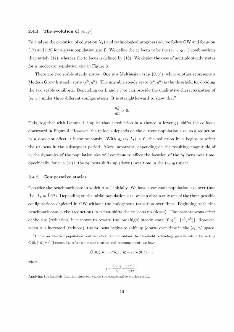
2.4.1 The evolution of (et; gt)

To analyze the evolution of education (et) and technological progress (gt), we follow GW and focus on

(17) and (18) for a given population size L. We de�ne the ee locus to be the (et+1; gt+1) combinations

that satisfy (17), whereas the tg locus is de�ned by (18). We depict the case of multiple steady states

for a moderate population size in Figure 3.

There are two stable steady states. One is a Malthusian trap�0; g`

�, while another represents a

Modern Growth steady state�eh; gh

�. The unstable steady state (eu; gu) is the threshold for dividing

the two stable equilibria. Depending on L and n, we can provide the qualitative characterization of

(et; gt) under three di¤erent con�gurations. It is straightforward to show that9

d�g

dn> 0:

This, together with Lemma 1, implies that a reduction in �n (hence, a lower �g), shifts the ee locus

downward in Figure 3. However, the tg locus depends on the current population size, so a reduction

in �n does not a¤ect it instantaneously. With gL (et; Lt) > 0, the reduction in �n begins to a¤ect

the tg locus in the subsequent period. More important, depending on the resulting magnitude of

�n, the dynamics of the population size will continue to a¤ect the location of the tg locus over time.

Speci�cally, for �n > (<)1, the tg locus shifts up (down) over time in the (et; gt) space.

2.4.2 Comparative statics

Consider the benchmark case in which n = 1 initially. We have a constant population size over time

(i.e. Lt = �L 8t). Depending on the initial population size, we can obtain only one of the three possible

con�gurations depicted in GW without the endogenous transition over time. Beginning with this

benchmark case, a rise (reduction) in n �rst shifts the ee locus up (down). The instantaneous e¤ect

of the rise (reduction) in n moves us toward the low (high) steady state�0; g`

�[�eh; gh

�]. However,

when n is increased (reduced), the tg locus begins to shift up (down) over time in the (et; gt) space.

9Under an e¤ective population control policy, we can obtain the threshold technology growth rate �g by setting

�G (0; �g; �n) = 0 (Lemma 1). After some substitution and rearrangement, we have

�G (0; �g; �n) = � qhe (0; �g)� "�eh (0; �g) = 0

where

" =1�

n� q

1� n� q .

Applying the implicit function theorem yields the comparative statics result.

10

We eventually converge on the stable high (low) steady state�eh; gh

�[�0; g`

�]. Although the two

loci change in opposite directions, the shift of the tg locus over time eventually dominates in the

benchmark case. This provides an illustration of the trade-o¤ e¤ects of population control policies

between the short and long run.

Now consider an alternative case in which population policy is reduced from �n > 1 to �n = 1 so

as to preserve a stable population size. The reduction of �n shifts the ee locus down, whereas the tg

locus remains stable at the current population size over time (see Figure 4). This is an example of

implementing a policy to replace the mechanism of natural evolution (the shift of the tg locus due

growth in the population over time) to achieve the same qualitative equilibrium outcome.

The higher the current population growth rate under population control (�n), the larger the

magnitude of the downward shift in the ee locus. Thus, e¤ective population control is more likely to

help a country escape the development trap and move to a stable high steady state�eh; gh

�.

Finally, suppose that we are at the Post-Malthusian stage in which population reaches a medium

size such that multiple steady states emerge. Given the introduction of the population control policy

represented by a reduction in �n, the �rst outcome is a downward shift in the ee locus. There are

three possible ultimate steady-state outcomes depending on the severity of the population control

policy. If the new population policy target is at �n = 1, we are very likely to achieve a stable new

higher steady state�eh; gh

�. This positive outcome is guaranteed when we have the possibility of

�n > 1. This is because the tg locus begins to shift up over time, and thus, the high steady state is a

certain equilibrium outcome. However, if the population control policy is su¢ ciently stringent that

�n < 1, then the �nal outcome is completely di¤erent. Although a large reduction in �n can shift the

ee locus down signi�cantly to where we are initially able to achieve the Modern Growth Regime, the

subsequent developments di¤er. When �n < 1, the tg locus also begins to shift down over time. With

this restricted level of �n, the �nal outcome must be the case in which the population size declines to

such a low level that we fall into the Malthusian trap.

2.5 Global dynamics

We now consider how population control policy governs the demographic transition and hence the

evolution of the economy from the Post-Malthusian Regime to the Modern Growth Regime. Following

GW, the global analysis is based on a sequence of phase diagrams that describe the evolution of the

system within each regime and the transition between the regimes on the (et; xt) dimension. The

11

phase diagrams contain two elements: the XX locus, which denotes the set of all pairs (et; xt) for

which e¤ective resources per worker are constant (xt+1 = xt, 8t), and the EE locus, which denotes

the set of all pairs (et; xt) for which the level of education per worker is constant (et+1 = et, 8t).

We �rst derive the XX locus, which is given by

xt+1 = xt () 1 + g (e; Lt) = n .

It is a vertical curve in the (et; xt) space located at et = e. Without delving excessively into analytical

detail, we simply make the following assumption for e:

Assumption A3 �g < g (e; L) < gh�eh; L

�.

We then conclude

xt+1 > xt if et > e

xt+1 = xt if et = e

xt+1 < xt if et < e .

Furthermore, for a reduction (rise) in �n, the XX locus shifts to the left (right).

Next, for the EE locus, we have

EE � f(et; xt) : et+1 = etg

or et+1 = e (g (et; Lt) ;n) .

For a given population size, the steady-state values of et are independent of xt. Thus, the EE locus is

again a vertical line in the (et; xt) space, the location of which depends on the size of the population

L (which in turn determines the relative positions of the ee locus and the tg locus). The e¤ects of a

change in n on its location operate through the interactions of the ee locus and the tg locus. Overall,

we have three possible cases of steady-state equilibria for any given level of population size and �n.

2.6 Conditional steady-state equilibria

We apply our global dynamic analysis to the benchmark case in which n > 1 such that the size of

the population evolves naturally over time. Suppose that a tightening of n to unity is e¤ective when

the population size is at its intermediate level, at which multiple equilibria are present (see Figure

5).

12

The instantaneous e¤ect is that the ee locus in Figure 4 shifts down, meaning that the high

steady state (eh; gh) moves to the right, whereas the low steady state (eu; gu) moves to the left. As

a result, the EE locus (et+1 = et, 8t) located at eu (eh) shifts left (right), whereas the XX locus

(xt+1 = xt, 8t) shifts left. Thus, the region where the law of motion indicates a convergence toward

eh expands. The limiting case is the situation where the EE locus located at eu coincides with the

vertical axis so that et = eh.

The above analysis of global dynamics can be completely di¤erent if the population control

policy is stringent enough to achieve n < 1, leading to a decline in the population size over time.

The instantaneous e¤ect again is that the ee locus in Figure 4 shifts down, but the reduction in L

also shifts down the tg locus over time. The location of the steady states begins to reverse: the high

steady state (eh; gh) moves to the left, whereas the low steady state (eu; gu) moves to the right. In

the phase diagram, this is also re�ected in the reversed movements of both the EE and XX loci: the

EE locus located at eu (eh) shifts right (left), whereas the XX locus shifts right. As a result, the

region where et+1 > et shrinks over time and eventually vanishes so that education can only decline

over time. Other things being equal, we are ultimately converging to the Malthusian steady-state

equilibrium of et = 0. Thus, a permanent population control policy that ultimately yields (n < 1)

must be harmful.

Our analysis reveals that there is an instantaneous or short-run gain from restricting population

growth that allows the economy to move toward the high-growth steady state. Qualitatively, a

compromise to improve the overall situation seems to involve tightening the restriction on population

growth for a certain period of time (i.e. temporarily) and then relaxing the restriction to prevent a

decline in the population size over time.

3 Quantitative analysis of China�s OCP

China introduced its OCP in 1979 with the aim of increasing resources per capita and facilitating

China�s economic reforms. Under the policy, each family was limited to a single child, with penalties

imposed for subsequent births. The OCP successfully reduced the average annual population growth

rate from the 1:87% (observed from 1960 to 1979) to the 1:28% (observed from 1980 to 1999).

Before the formal announcement of the OCP, premier Zhou Enlai initiated a nationwide campaign

in the 1970s that called upon cadres at all administrative levels to promote population control.

Later marriage, longer intervals between births, and fewer children were advocated. The o¢ cially

13

stated means of policy implementation were education, propaganda, and mild persuasion. While

this approach to population control policy resulted in a decline in the population growth rate in the

early 1970s, more aggressive measures seen necessary. In 1979, the Chinese government o¢ cially

announced the OCP.10

In this section, we introduce a numerical version of the model to study the quantitative e¤ects of

the OCP. To proceed, we specify the functional forms for the technology and preferences of the basic

model à la Lagerlöf (2003, 2006). Then we choose the parameterization following common practice

in the literature. We also propose a welfare analysis for assessing the OCP. Finally, we graphically

present our �ndings of the e¤ects of the OCP on growth and welfare.

3.1 Functional forms

Following Lagerlöf (2003, 2006), we set � q = � and � e = 1. The human capital accumulation function

is speci�ed as

ht+1 = h (et+1; gt+1) =et+1 + ��

et+1 + �� + gt+1,

where � 2 (0; 1) denotes the relative time cost of having a child, and hence, et+1+�� can be regarded

as the e¤ective level of education. Furthermore, technological progress gt+1 takes the form

gt+1 = g (et; Lt) = (et + ��) a (Lt)

where a (Lt) is the scale e¤ect determined by

a (Lt) = min f�Lt; a�g

where � and a� are both positive scale parameters. Therefore, the education dynamics et+1 are a

function of et and Lt.

De�nition 1 The recursive system is de�ned by three dynamic equations on gt+1, At+1 and Lt+1

and two speci�c equations for et+1 and nt under the population control policy in the Post-Malthusian

Regime:

gt+1 = (et + ��) at ,

At+1 = (1 + gt+1)At ,

Lt+1 = ntLt ,

10See Yang and Chen (2004) and Liao (2013) for a detailed review of the OCP in China.

14

where

at = min f�Lt; a�g .

When population control policy is not in e¤ect (i.e. natural evolution is allowed), education and

fertility choices are determined by

et+1 = maxn0;p(1� �) �gt+1 � ��

o

nt =

8<:

�+et+1if zt � ec

1� 1�ec=zt�+et+1

if zt < ec1�

where

zt =

�et + ��

et + �� + gt

���AtXLt

�1��.

When the OCP is in e¤ect, education and fertility choices are determined by

et+1 = max

(0;

s�"�1 +

�

1�

��gt+1 +

�]

gt+1

�2 (1� )2 �

��� +

gt+12 (1� )

�)

nt = n

both for given initial values of L0, e0, and n0, together with the parameters a�, �, � , �, , �, X, ec.3.2 Parameterization

Following the suggestion of Boldrin and Jones (2002), we de�ne the length of a generation to be 20

years. The labor share of output � is set to be 0:443, which is estimated using employee compensation

as a fraction Chinese GDP.11 The time devoted to education in the Modern Growth Regime e� equals

7:5%, the world average, whereas the fertility rate in the Modern Growth Regime n� is normalized

to 1, and the initial population L0 to be 0:364 (Lagerlöf, 2006). We also set the �xed time cost � at

0:15, which is the same as the US value.12

In the uni�ed growth framework, we concentrate on the interaction between the demographic

transition and the take-o¤ from the Post-Malthusian Regime to the Modern Growth Regime. To

11This is based on the Income Approach Components of the Gross Regional Product Table from the National Bureau

of Statistics of China. Another reference for a detailed analysis of the factor income distribution in China is Bai and

Qian (2009).12See the detailed discussion on choosing e�, n� and � (Lagerlöf, 2006). Here we implicitly assume that the education

time e�, fertility rate n�, and the education time � in the Modern Growth Regime are identical for all countries. In

other words, all countries converge to the same steady-state over the long run.

15

highlight the e¤ect of population control policy, we assume that the OCP is the only e¤ective policy

factor that in�uences China economic growth in this period.13 We calibrate the target value of the

technology growth rate in the Modern Growth Regime g� and the timing of imposing the OCP to

match two certain key data moments of the Chinese experience. These key moments are the timing

of implementing OCP in China, i.e. the �nal generation of the Post-Malthusian period (say, 35th

generation); and the per-adult income growth rate, which is 6% after 40 years (two generations) of

OCP. From this, we back out the steady-state growth rate of technology g� and the per capita GDP

under natural evolution. These values are 17:5541 and 8:94%, respectively.

Having obtained values for g� and e�, we can solve a� and � from the equations for the Modern

Growth Regime

g� = a�2� (1� �) ,

e� = a�� (1� �)� �� .

The parameter is set such that population is constant in the Modern Growth Regime, i.e.

n� = = (� + e�).

We assume that the population control parameter n = 1 is such that the population size does

not decline when the OCP is in e¤ect. Following Lagerlöf (2006), the remaining parameters such as

�, X, and ec are all normalized to one.For the initial values, we also follow the method used in Lagerlöf (2006). We assume that the

education level e0 is zero and, hence, that the initial technology is g0 = ���L0. The income equals

the subsistence level such that z0 = ec= (1� �). From the production function, we can solve for A0

for a given z0, L0, X, �, and �. The remaining parameters (�, X, and ec) are all normalized to 1. Weprovide a summary of the parameterization in Table 1.

3.3 Welfare

In addition to Lagerlöf�s quantitative analysis of demographics and growth, we provide a welfare

assessment of the OCP along the lines of Song et al. (2015). We assess the welfare e¤ects of the

permanent and the temporary OCP. To compute the welfare cost of the OCP relative to natural

13China implemented many reforms in the late 1970s, including the Opening Up Policy, the restoration of national

college entrance examination, and the abolition of the people�s communes, etc. All these reforms had great impact on

the factor productivity and contributed to China�s economic growth. Here, we concentrate on the growth e¤ect of the

demographic transition, i.e. the sphere in which the OCP had its most profound e¤ect.

16

evolution, we follow the standard criterion of adopting the (socially) discounted lifetime utility of

the representative household under regime j (either OCP or natural evolution):

V j0 =1Xt=0

�tLjtujt

�cjt ; n

jt ; h

jt+1

�where � 2 (0; 1) is the social discount factor across generations and ujt

�cjt ; n

jt ; h

jt+1

�= (1� ) ln cjt +

ln�njth

jt+1

�is given by (4). Thus, the equivalent variation is obtained from ! in the following

speci�cation:

1Xt=0

�tLNEt uNEt�(1 + !) cNEt ; nNEt ; hNEt+1

�=

1Xt=0

�tLOCPt uOCPt

�cOCPt ; nOCPt ; hOCPt+1

�where ! < 0 measures the welfare loss due to the implementation of the OCP. The choice of the

social discount factor � is crucial for the analysis. Following Song et al. (2015), we employ � = 0:975

for our hypothetical planner.

3.4 Findings

3.4.1 The permanent OCP case

From the calibration, once the OCP is implemented (nt = �n = 1), the instantaneous e¤ect is a

corresponding jump in GDP per capita. Population control promotes strong growth in GDP per

capita in the short run. This �nding is consistent with our theoretical prediction and the empirical

results of Li and Zhang (2007). In the benchmark case, as shown in Figure 6, the timing of the

imposition of the OCP is chosen to be the 35th generation, i.e. the �nal generation of the Post-

Malthusian era. When the OCP is implemented, a critical mass of population cannot be accumulated

due to zero population growth. This reduces growth performance in the steady state. However,

Figure 6 also shows that education begins to increase once the OCP is implemented. This implies

that the OCP causes agents to experience the quantity-quality trade-o¤ earlier than under natural

evolution. This is because the reduction in �n reduces the threshold level of technological growth (�g)

such that it pays to acquire education. However, once the quantity-quality trade-o¤ begins under

natural evolution, the relative gain in per capita income growth under OCP vanishes.

From the analysis, we can see that the OCP in China yields higher economic growth than does

natural evolution for more than two generations (40+ years), owing to both the instantaneous e¤ect

of a smaller population base and a higher education level resulting from an earlier quantity-quality

trade-o¤. Speci�cally, the per capita income growth rates are 5:82% and 6% for the 36th and

17

37th generations under permanent OCP, whereas they are 3:64% and 5:12%, respectively, under

natural evolution. The policy�s long-run cost is much higher, however, with a 22% decline in per

capita GDP growth in the steady state (6:95% under permanent OCP versus 8:94% under natural

evolution), due to the lower population mass and education in the steady state. In fact, growth

under natural evolution is higher than growth under OCP starting from the third generation after

the implementation of the policy.

Moreover, the earlier the government imposes the OCP, the lower the resulting GDP per capita

growth rate. This is consistent with our uni�ed growth theory of OCP. The earlier the OCP is

implemented, the less likely we are to achieve critical mass in the labor force, thereby magnifying

the negative quantity e¤ect on growth relative to the positive quantity-quality trade-o¤ e¤ect.

To see this, we perform two OCP experiments. We �rst impose the OCP one generation earlier

(34th generation). Figure 7 shows that the trade-o¤ between the short-run gain and long-run cost

rises signi�cantly. However, if we postpone the OCP for one generation such that it is imposed

during the Modern Growth Period (36th generation), then the trade-o¤ between the short-run gain

and long-run cost diminishes. This con�rms our intuition that delaying the implementation of the

OCP reduces the negative quantity e¤ect and increases the positive quantity-quality trade-o¤ e¤ect.

Summary 1 The OCP promotes growth in the short run, but retards it in the steady state. The

earlier the OCP is imposed, the higher its long-run cost in terms of lower growth.

3.4.2 The temporary OCP case

The Chinese central government recently abandoned the OCP by allowing each family to have two

children. For analytical convenience, we can regard this as the situation in which the population

constraint is non-binding. Thus, we can study the suspension of the OCP by treating the original

OCP as a temporary policy that lasted for two generations (approximately 40 years, 1979�2016).

We illustrate the e¤ects of China�s temporary OCP in Figure 8.

Figure 8 shows that the economy enjoys higher income growth relative to natural evolution for

two generations, then falls behind and ultimately returns to the same steady-state level. Notably,

when population growth rebounds, per capita income growth declines. The duration of the transition

is essentially identical to that under natural evolution. As shown in Figure 8, population growth with

a temporary OCP is higher than that under natural evolution for a few generations in transition.

This intuitively makes sense; a critical population mass has to be achieved under the temporary

18

OCP to obtain the same steady-state level of income growth. The temporary OCP exhibits more

�uctuations in income growth than does the permanent OCP. This is due to the �uctuations in

population growth because the economy has to make up for the loss in population due to the OCP

after it has been abandoned. In addition, as in the permanent OCP case, the quantity-quality trade-

o¤ begins to be e¤ective once the OCP is in e¤ect. However, once the OCP is lifted, the quantity-

quality trade-o¤ is reversed. Thus, the quantity-quality trade-o¤ �uctuates under the temporary

OCP, whereas it is monotone under natural evolution.

The temporary OCP extends for the duration of the Post-Malthusian period and delays the

emergence of the Modern Growth period. This is intuitive because the temporary OCP delays the

accumulation of the critical mass of population in the uni�ed growth model.

Our calibration shows that the OCP is reversible since the natural evolution of the economy is

restored after the policy is removed. However, it also highlights the fact that the two-generation

gain in income growth under the temporary OCP comes at the expense of approximately eight

generations of lower growth. Nevertheless, our quantitative exercise shows that any temporary

policy on population in the GW model does not have a permanent e¤ect on long-run growth.

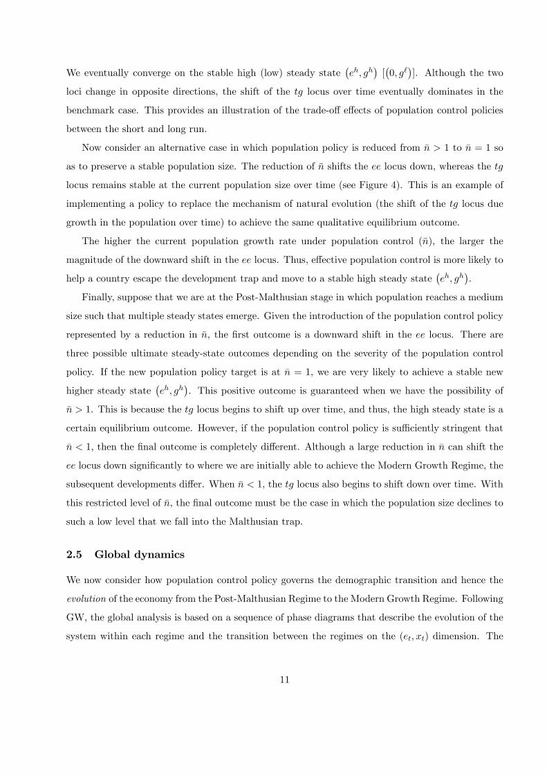
Before concluding our analysis on the temporary OCP, we study the e¤ect of the duration of

the temporary OCP. Figure 9 shows that the longer the duration of the temporary OCP, the larger

its deviation from the benchmark of natural evolution. For instance, if we delay the removal of the

OCP for one more generation (i.e. temporary policy lasts three generations), the relative decline

in per capita income growth from the natural-evolution level is much more substantial during the

transition.

Summary 2 Once the OCP is removed, the economy reverts to the steady state under natural evolu-

tion. Population growth, per capital income growth, and education all �uctuate during the transition,

and the emergence of the Modern Growth era is delayed. The longer the duration of the temporary

OCP, the lower per capita income growth in transition.

3.4.3 Welfare

We now assess the welfare consequences by solving for the equivalent consumption variation of the

OCP relative to natural evolution. Both temporary and permanent OCPs give rise to an initial

welfare gain for less than two generations in return for a subsequent permanent welfare loss (see

Figure 10).

19

Welfare is reduced even when per capita income growth is above its level under natural evolution

in the short run. The reason is that the population level at the time when the OCP is implemented

is too low (LNEt > LOCPt ). Although the OCP promotes short-run growth, it reduces welfare. The

demographic factor plays a crucial role in determining overall welfare. Furthermore, as shown in

Figure 10, if the OCP is temporary, its adverse e¤ect on the population mass is less, so the welfare

loss is smaller. This makes sense; population growth, education level, and per capita income growth

are lower in the steady state in the permanent OCP case than in the temporary OCP case. The

latter approaches the same steady state as in the case of natural evolution.

Now suppose we postpone the OCP by one generation. We know that the cost in terms of growth

is smaller because the initial population mass is larger, and thus, the deviation from natural evolution

is smaller. In terms of welfare cost, the intuition carries over to the case of a permanent OCP, except

that we have no short-run gain due to the restriction of the population mass by the OCP. When we

postpone the OCP, the welfare loss in the short run is higher for four generations but the subsequent

loss is smaller. This is consistent with our �ndings on the e¤ects of the OCP on economic growth.

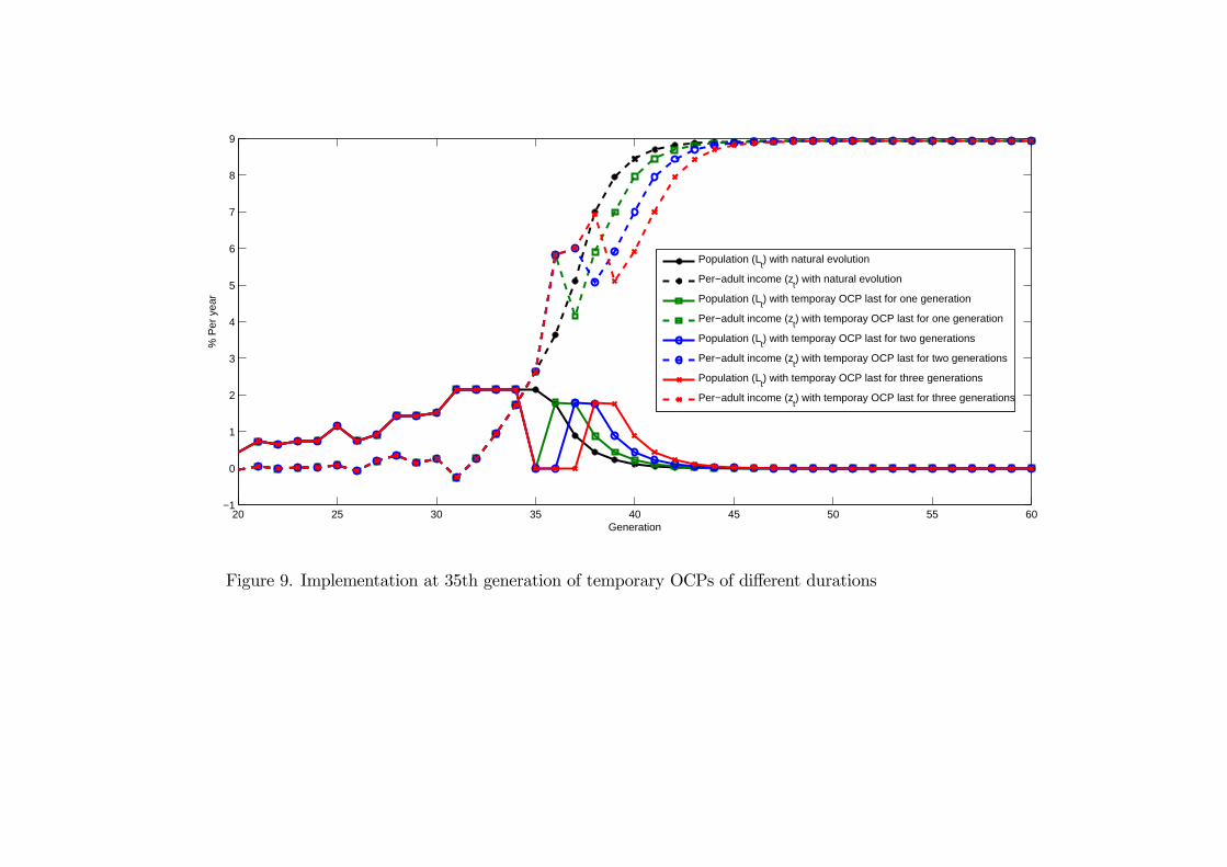
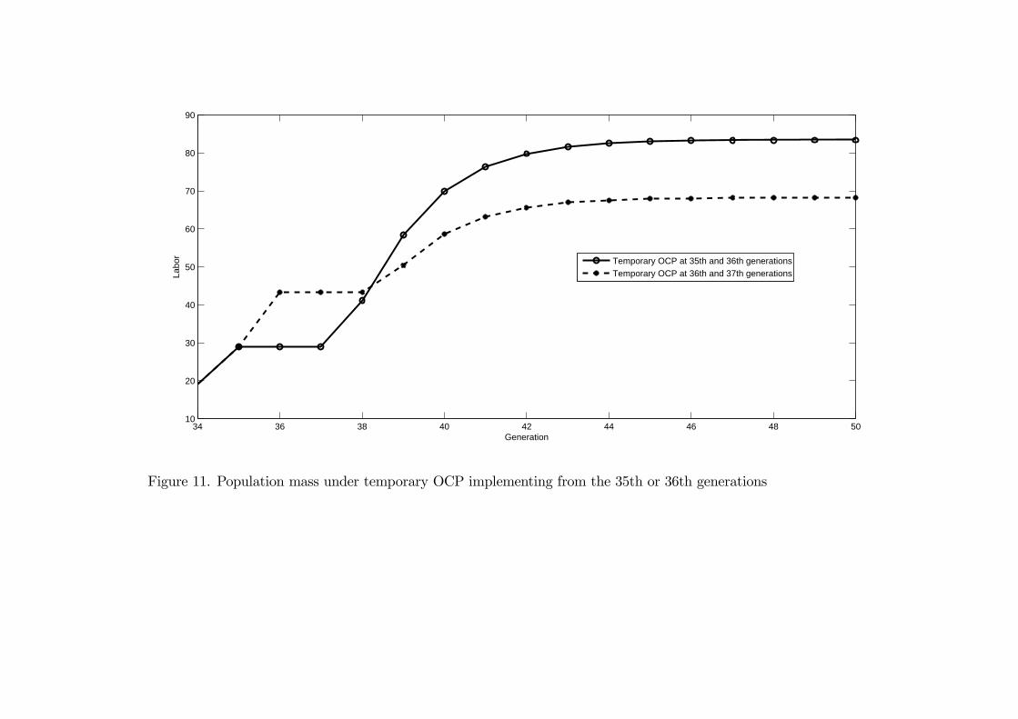
Figure 11 presents an interesting observation on postponing the temporary OCP for a generation.

Again, we observe welfare loss for the entire time path due to the delay of OCP implementation.

However, the welfare loss is exacerbated over time when the OCP is temporary. To understand this

result, we note that population growth rebounds in the benchmark temporary OCP case after the

policy is abandoned. As a result, the steady-state population mass achieves nearly the same level

as under natural evolution. However, when the OCP is imposed during the Modern Growth era

(36th generation), the initial population mass is higher and the initial population growth rate is

lower than in the benchmark case. After two generations, when the OCP is eliminated, the rate

at which population growth rebounds is reduced such that the population mass in the steady state

is lower than the initial level (see Figure 11). This is the source of the welfare loss over the entire

horizon considered relative to the benchmark case. This intuition concerning the adjustment of the

population mass can be applied to understand the welfare cost of the duration of the temporary

OCP. The longer the temporary OCP lasts, the smaller the population mass. Therefore, as shown

in Figure 12, the welfare loss increases with the duration of the temporary OCP.

Summary 3 The OCP reduces welfare. The welfare loss from the temporary OCP is smaller than

that from the permanent OCP. Delaying the implementation of the permanent OCP always results

in a trade-o¤ between a higher short-run loss and a lower long-run cost. In the case of the temporary

20

OCP (depending on the timing of the implementation relative to the Modern Growth era), there can

be no welfare gain for delaying the OCP. The welfare cost increases with the policy�s duration.

4 Concluding remarks

This paper extended the GW (2000) model by introducing a population constraint to understand the

role of the OCP on China�s economic growth and demographic transition. Qualitatively, the OCP

promotes growth in the short run, but reduces it in the steady state. The earlier the imposition of

the OCP, the lower the economic growth. From the calibration, we found that without the OCP, the

steady-state growth rate of per capita GDP under natural evolution is approximately 8:94%. Other

things being equal, a permanent OCP in China delivers higher economic growth for approximately

two generations, but its long-run cost is much higher. Ultimately, it results in a 22% reduction in

per capita GDP growth in the steady state.

We also considered the Chinese government�s recent decision to move to a two-child policy. By

allowing each family to have two children, the original OCP becomes a temporary policy that lasted

for two 20-year generations. After rising for two consecutive generations, per capita GDP growth

declines and slowly returns to the level that would be observed under natural evolution. Relative to

its absence, the OCP creates a trade-o¤ in growth between a gain for the �rst two generations and a

loss afterwards. In addition, following the methodology of Song et al. (2015), we assess the welfare

cost of the OCP. We �nd that the welfare cost over time is always higher for the permanent OCP

than the temporary OCP.

We also provided a few counterfactual exercises. On one hand, hastening implementation of a

permanent OCP increases the adverse e¤ect on growth. On the other hand, delaying the time when

the temporary OCP is lifted leads to weaker economic growth over time. Both of these counterfactuals

imply a larger reduction in the population mass such that the adverse e¤ect on growth is larger. In

terms of welfare, the �ndings are robust in that both exercises yield a higher welfare loss over

time. An interesting and important �nding from our counterfactuals is that the welfare cost of the

temporary OCP is very sensitive to its timing relative to the Modern Growth era. We �nd that if we

impose the temporary OCP when the economy enters the Modern Growth Regime, we can be worse

o¤ both in the short run and in the steady state. Again, the intuition is based on the adjustment

of the population mass in response to the OCP. In light of these demographic and macroeconomic

implications, policymakers should be quite cautious in pursuing population restrictions.

21

This paper focused on the demographic change of the macroeconomy caused by the OCP, and

was based on a belief that the �rst-order e¤ect of OCP must fall on the population. For the sake

of tractability, we abstract from many factors of China growth noted in the literature, including

savings, investment, openness, capital �ows, as well as external and internal trade. We believe that

some of the e¤ects from these factors can be captured in the total factor productivity (TFP) term of

production technology. As discussed in Lagerlöf (2006), most quantitative �ndings of the GW model

do not change qualitatively when TFP changes. However tantalizing, investigation into how these

factors interact with the OCP must remain a matter for future research.

22

References

[1] Bai, C., Qian, Z., 2009. Factor income share in China: The story behind the statistics (in

Chinese). Econ. Res. J. 3, 27-41.

[2] Barlow, R., 1994. Birth rate and economic growth: Some more correlations. Popul. Dev. Rev.

20, 153-165.

[3] Barro, R.J., Becker, G.S., 1989. Fertility choice in a model of economic growth. Econometrica

57, 481-501.

[4] Becker, G.S., Murphy, K.M., Tamura, R.F., 1990. Human capital, fertility, and economic growth.

J. Political Econ. 98, S12-S37.

[5] Boldrin, M., Jones, L.E., 2002. Mortality, fertility, and saving in a Malthusian economy. Rev.

Econ. Dyn. 5, 775-814.

[6] Brander, J.A., Dowrick, S., 1994. The role of fertility and population in economic growth: New

results from aggregate cross-national data. J. Popul. Econ. 7, 1-25.

[7] Coale, A., 1986. Population trends and economic development, in: Menken, J. (ed.), World

Population and US Policy: The Choice Ahead. W. W. Norton, New York, pp. 96-104.

[8] Galor, O., 2005. From stagnation to growth: Uni�ed growth theory, in: Aghion, P., Durlauf, S.

(eds.), Handbook of Economic Growth. North-Holland, Amsterdam, pp. 171-293.

[9] Galor, O., Weil, D.N., 1996. The gender gap, fertility, and growth. Am. Econ. Rev. 86, 374-387.

[10] Galor, O., Weil, D.N., 2000. Population, technology, and growth: From Malthusian stagnation

to the demographic transition and beyond. Am. Econ. Rev. 110, 806-828.

[11] Hazledine, T., Moreland, R.S., 1977. Population and economic growth: A world cross-section

study. Rev. Econ. Stat. 59, 253-263.

[12] Kelley, A.C., 1988. Economic consequences of population change in the Third World. J. Econ.

Lit. 26, 1685-1728.

[13] Kelley, A.C., Schmidt, R.M., 1994. Population and income change: Recent evidence. World

Bank Discussion Paper 249.

23

[14] Kelley, A.C., Schmidt, R.M., 1995. Aggregate population and economic growth correlations:

The role of the components of demographic change. Demography 32, 543-555.

[15] Lagerlöf, N.P., 2003. From Malthus to modern growth: Can epidemics explain the three regimes?

Int. Econ. Rev. 44, 755-777.

[16] Lagerlöf, N.P., 2006. The Galor-Weil model revisited: A quantitative exercise. Rev. Econ. Dyn.

9, 116-142.

[17] Li, H., Zhang, J., 2007. Do high birth rates hamper economic growth? Rev. Econ. Stat. 89,

110-117.

[18] Liao, P-J., 2011. Does demographic change matter for growth? Eur. Econ. Rev. 55, 659-677.

[19] Liao, P-J., 2013. The one-child policy: A macroeconomic analysis. J. Dev. Econ. 101, 49-62.

[20] Maddison, A., 2003. The World Economy: Historical Statistics. Organisation for Economic

Co-operation and Development, Paris.

[21] Maddison, A., 2007. Chinese Economic Performance in the Long Run: 960-2030 AD. Organi-

sation for Economic Co-operation and Development, Paris.

[22] Malthus, T.R., 1826. An Essay on the Principle of Population, sixth ed. Cambridge University

Press, Cambridge, UK.

[23] McNicoll, G., 1984. Consequences of rapid population growth: An overview and assessment.

Popul. Dev. Rev. 10, 537-544.

[24] Rosenzweig, M.R., Zhang, J., 2009. Do population control policies induce more human capital

investment? Twins, birthweight, and China�s one child policy. Rev. Econ. Stud. 76 (3), 1149-

1174.

[25] Simon, J.L. 1989. On aggregate empirical studies relating population variables to economic

development. Popul. Dev. Rev. 15, 323-332.

[26] Song, M. Z., Storesletten, K., Wang, Y., Zilibotti, F., 2015. Sharing high growth across genera-

tions: pensions and demographic transition in China. Am. Econ. J. Macroecon. 7 (2), 1-39.

[27] Temple, J., 1999. The new growth evidence. J. Econ. Lit. 37, 112-156.

24

[28] Yang, D.T., Chen, D., 2004. Transformations in China�s population policies and demographic

structure. Pac. Econ. Rev. 9 (3), 269-290.

[29] Zhu, X., 2012. Understanding China�s growth: Past, present, and future. J. Econ. Perspect. 26

(4), 103-124.

25

Table 1: Parameter values

Interpretation Value

Parameters

α Labor share 0.443

τ Fixed time cost of raising children 0.15

ρ Educational part of τ 0.9813

a∗ Scale effect parameter 79

γ Weight on fertility in utility function 0.225

θ Scale effect parameter 1

X Land 1

c Subsistence consumption 1

Endogenous variables

e∗ Education, modern growth 0.075

g∗ Technological growth, modern growth 17.554

n∗ Fertility, modern growth 1

L Threshold population 52.337

Initial conditions

n0 Initial fertility 1

L0 Initial population 0.364

A0 Initial technology 0.6236

e0 Initial education 0

g0 Initial technological growth 0.0536

z0 Initial per-worker income 1.176

Potential GDP growth rate 8.94

Figure  1  Growth  rates  in  Western  Europe  (Lagerlof,  2006) �

Source: Maddison (2003), Maddison (2007).

Figure 2 Growth rates in China estimated by Maddison

1500-1700 1701-1850 1851-1913 1914-1950 1951-1961 1962-1976 1977-1992 1993-2003GDP Per Capita Growth 0 0 -0.13 -0.62 1.52 3.14 5.85 7.75Population Growth 0.15 0.73 0.09 0.61 1.71 2.42 1.42 0.9

-2

-1

0

1

2

3

4

5

6

7

8

%

Population Growth GDP Per Capita Growth

gh

gu

gl

eu eh

gt

et

tg

ee

0

Figure 3. The evolution of technology and education for a moderate population size

gl �

gt�

et�

tg�

ee1�

0�

ee2�

he1 he2

hg1

hg2

Figure  4  The  effect  of  OCP  where            is  reduced  to  1�n

e e∗ eEducation, et

Effective resources p

er worker, x t

Figure 5. The conditional dynamical system for a moderate population size

20 25 30 35 40 45 50 55 60−1

0

1

2

3

4

5

6

7

8

9

Generation

% P

er y

ear

Population (Lt) with permanent OCP

Per−adult income (zt) with permanent OCP

Education*100 (et*100) with permanent OCP

Population (Lt) with natural evolution

Per−adult income (zt) with natural evolution

Education*100 (et*100) with natural evolution

Figure 6. Implementation of permanent OCP at 35th generation

20 25 30 35 40 45 50 55 60−1

0

1

2

3

4

5

6

7

8

9

Generation

% P

er y

ear

Population (Lt) with natural evolution

Per−adult income (zt) with natural evolution

Population (Lt) with permanent OCP from 34th generation

Per−adult income (zt) with permanent OCP from 34th generation

Population (Lt) with permanent OCP from 35th generation

Per−adult income (zt) with permanent OCP from 35th generation

Population (Lt) with permanent OCP from 36th generation

Per−adult income (zt) with permanent OCP from 36th generation

Figure 7. Implementations of permanent OCP at 34th, 35th, and 36th generations

20 25 30 35 40 45 50 55 60−1

0

1

2

3

4

5

6

7

8

9

Generation

% P

er y

ear

Population (Lt)

Per−adult income (zt)

Education*100 (et*100)

Population (Lt) with natural evolution

Per−adult income (zt) with natural evolution

Education*100 with natural evolution

Figure 8. Implementation of temporary OCP at 35th and 36th generations

20 25 30 35 40 45 50 55 60−1

0

1

2

3

4

5

6

7

8

9

Generation

% P

er y

ear

Population (Lt) with natural evolution

Per−adult income (zt) with natural evolution

Population (Lt) with temporay OCP last for one generation

Per−adult income (zt) with temporay OCP last for one generation

Population (Lt) with temporay OCP last for two generations

Per−adult income (zt) with temporay OCP last for two generations

Population (Lt) with temporay OCP last for three generations

Per−adult income (zt) with temporay OCP last for three generations

Figure 9. Implementation at 35th generation of temporary OCPs of different durations

0 2 4 6 8 10 12 14 16−1

−0.9

−0.8

−0.7

−0.6

−0.5

−0.4

−0.3

−0.2

−0.1

0

0.1

Period

Wel

fare

equ

ival

ent

Permanent OCP from the 35th generationTemporary OCP at 35th and 36th generationsPermanent OCP from the 36th generationTemporary OCP at 36th and 37th generations

Figure 10. Welfare equivalent under permanent and temporary OCP from the 35th and 36th generations

34 36 38 40 42 44 46 48 5010

20

30

40

50

60

70

80

90

Generation

Labo

r

Temporary OCP at 35th and 36th generationsTemporary OCP at 36th and 37th generations

Figure 11. Population mass under temporary OCP implementing from the 35th or 36th generations

34 36 38 40 42 44 46 48 50−0.9

−0.8

−0.7

−0.6

−0.5

−0.4

−0.3

−0.2

−0.1

0

0.1

Generation

Wel

fare

equ

ival

ent

Temporary OCP lasting for two generationsTemporary OCP lasting for three generationsTemporary OCP lasting for four generations

Figure 12. Welfare equivalent under temporary OCPs lasting for 2, 3 and 4 generations

BOFIT Discussion Papers A series devoted to academic studies by BOFIT economists and guest researchers. The focus is on works relevant for economic policy and economic developments in transition / emerging economies.

BOFIT Discussion Papers http://www.bofit.fi/en • email: bofit@bof.fi

ISSN 1456-4564 (print) // ISSN 1456-5889 (online)

2016 No 1 Guonan Ma and Wang Yao: Can the Chinese bond market facilitate a globalizing renminbi? No 2 Iikka Korhonen and Riikka Nuutilainen: A monetary policy rule for Russia, or is it rules? No 3 Hüseyin Şen and Ayşe Kaya: Are the twin or triple deficits hypotheses applicable to post-communist countries? No 4 Alexey Ponomarenko: A note on money creation in emerging market economies No 5 Bing Xu, Honglin Wang and Adrian van Rixtel: Do banks extract informational rents through collateral? No 6 Zuzana Fungáčová, Anastasiya Shamshur and Laurent Weill: Does bank competition reduce cost of credit? Cross-country evidence from Europe No 7 Zuzana Fungáčová, Iftekhar Hasan and Laurent Weill: Trust in banks No 8 Diana Ayala, Milan Nedeljkovic and Christian Saborowski: What slice of the pie? The corporate bond market boom in emerging economies No 9 Timothy Frye and Ekaterina Borisova: Elections, protest and trust in government: A natural experiment from Russia No 10 Sanna Kurronen: Natural resources and capital structure No 11 Hongyi Chen, Michael Funke and Andrew Tsang: The diffusion and dynamics of producer prices, deflationary pressure across Asian countries, and the role of China No 12 Ivan Lyubimov: Corrupt bureaucrats, bad managers, and the slow race between education and technology No 13 Tri Vi Dang and Qing He: Bureaucrats as successor CEOs No 14 Oleksandr Faryna: Exchange rate pass-through and cross-country spillovers: Some evidence from Ukraine and Russia No 15 Paul D. McNelis: Optimal policy rules at home, crisis and quantitative easing abroad No 16 Mariarosaria Comunale and Heli Simola: The pass-through to consumer prices in CIS economies: The role of exchange rates, commodities and other common factors No 17 Paul Castañeda Dower and William Pyle: Land rights, rental markets and the post-socialist cityscape No 18 Zuzana Fungáčová, Ilari Määttä and Laurent Weill: What shapes social attitudes toward corruption in China? Micro-level evidence No 19 Qing He, Jiyuan Huang, Dongxu Li and Liping Lu: Banks as corporate monitors: Evidence from CEO turnovers in China No 20 Vladimir Sokolov and Laura Solanko: Political influence, firm performance and survival

2017 No 1 Koen Schoors, Maria Semenova and Andrey Zubanov: Depositor discipline in Russian regions: Flight to familiarity or trust in local authorities? No 2 Edward J. Balistreri, Zoryana Olekseyuk and David G. Tarr: Privatization and the unusual case of Belarusian accession to the WTO No 3 Hongyi Chen, Michael Funke, Ivan Lozev and Andrew Tsang: To guide or not to guide? Quantitative monetary policy tools and macroeconomic dynamics in China No 4 Soyoung Kim and Aaron Mehrotra: Effects of monetary and macroprudential policies – evidence from inflation targeting economies in the Asia-Pacific region and potential implications for China No 5 Denis Davydov, Zuzana Fungáčová and Laurent Weill: Cyclicality of bank liquidity creation No 6 Ravi Kanbur, Yue Wang and Xiaobo Zhang: The great Chinese inequality turnaround No 7 Yin-Wong Cheung, Cho-Hoi Hui and Andrew Tsang: The Renminbi central parity: An empirical investigation No 8 Chunyang Wang: Crony banking and local growth in China No 9 Zuzana Fungáčová and Laurent Weill: Trusting banks in China No 10 Daniela Marconi: Currency co-movements in Asia-Pacific: The regional role of the Renminbi No 11 Felix Noth and Matias Ossandon Busch: Banking globalization, local lending, and labor market effects: Micro-level evidence from Brazil No 12 Roman Horvath, Eva Horvatova and Maria Siranova: Financial development, rule of law and wealth inequality: Bayesian model averaging evidence No 13 Meng Miao, Guanjie Niu and Thomas Noe: Lending without creditor rights, collateral, or reputation – The “trusted-assistant” loan in 19th century China No 14 Qing He, Iikka Korhonen and Zongxin Qian: Monetary policy transmission with two exchange rates and a single currency: The Chinese experience No 15 Michael Funke, Julius Loermann and Andrew Tsang: The information content in the offshore Renminbi foreign-exchange option market: Analytics and implied USD/CNH densities No 16 Mikko Mäkinen and Laura Solanko: Determinants of bank closures: Do changes of CAMEL variables matter? No 17 Koen Schoors and Laurent Weill: Russia's 1999-2000 election cycle and the politics-banking interface No 18 Ilya B. Voskoboynikov: Structural change, expanding informality and labour productivity growth in Russia No 19 Heiner Mikosch and Laura Solanko: Should one follow movements in the oil price or in money supply? Forecasting quarterly GDP growth in Russia with higher-frequency indicators No 20 Mika Nieminen, Kari Heimonen and Timo Tohmo: Current accounts and coordination of wage bargaining No 21 Michael Funke, Danilo Leiva-Leon and Andrew Tsang: Mapping China’s time-varying house price landscape No 22 Jianpo Xue and Chong K. Yip: One-child policy in China: A unified growth analysis