bolivia: selected issues - imf · 4 i. the natural gas sector and dutch disease 1 a. introduction...
TRANSCRIPT
© 2007 International Monetary Fund July 2007
IMF Country Report No. 07/249
Bolivia: Selected Issues
This Selected Issues paper for Bolivia was prepared by a staff team of the International Monetary Fund as background documentation for the periodic consultation with the member country. It is based on the information available at the time it was completed on June 29, 2007. The views expressed in this document are those of the staff team and do not necessarily reflect the views of the government of Bolivia or the Executive Board of the IMF. The policy of publication of staff reports and other documents by the IMF allows for the deletion of market-sensitive information.
To assist the IMF in evaluating the publication policy, reader comments are invited and may be sent by e-mail to [email protected].
Copies of this report are available to the public from
International Monetary Fund ● Publication Services 700 19th Street, N.W. ● Washington, D.C. 20431
Telephone: (202) 623 7430 ● Telefax: (202) 623 7201 E-mail: [email protected] ● Internet: http://www.imf.org
Price: $18.00 a copy
International Monetary Fund
Washington, D.C.

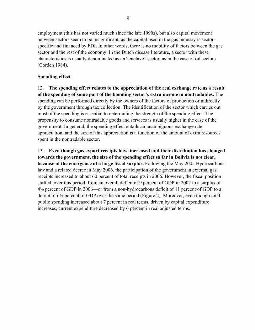
INTERNATIONAL MONETARY FUND
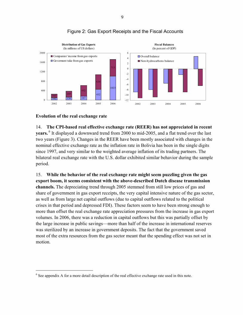
BOLIVIA
Selected Issues
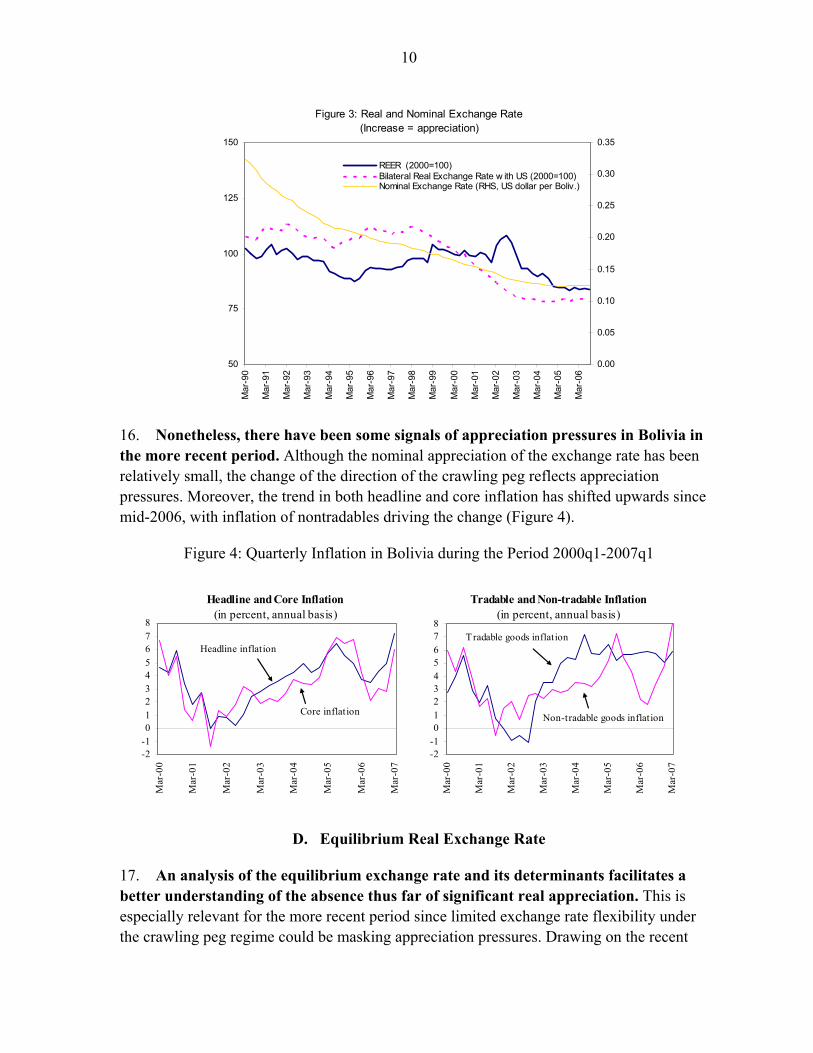
Prepared by Eugenio Cerutti, Laura Jaramillo, Mario Mansilla, Alejandro Simone, and Esteban Vesperoni
Approved by Western Hemisphere Department
June 29, 2007
Contents Page
I. The Natural Gas Sector and Dutch Disease ..........................................................................4 A. Introduction...............................................................................................................4 B. Bolivia’s Booming Natural Gas Sector.....................................................................5 C. Dutch Disease Risks..................................................................................................6 D. Equilibrium Real Exchange Rate............................................................................10 E. Concluding Remarks ...............................................................................................17
II. Tax System: Structure and Reform Options ......................................................................22 A. Introduction.............................................................................................................23 B. Tax System: Structure and Recent Developments ..................................................24 C. Key Tax Policy Issues .............................................................................................25 D. Reform Options.......................................................................................................29
III. Monetary Policy Transmission in Bolivia .........................................................................34 A. Introduction .............................................................................................................34 B. Institutional Context and Key Monetary Trends.....................................................35 C. Monetary Policy Transmission Channels................................................................36 D. Empirical Analysis..................................................................................................39 E. Conclusions and Policy Implications ......................................................................44
IV. Recent Experience with Debt Management .....................................................................45 A. Introduction .............................................................................................................45 B. Domestic Debt: Institutional Arrangements............................................................46 C. Recent Trends in Public Domestic Debt .................................................................47 D. Yields on Public Securities .....................................................................................53 E. Regional Comparisons.............................................................................................55 F. Currency Composition and Maturity: The Role of Economic Fundamentals .........56 G. Conclusions.............................................................................................................59
2
V. Long Term Management of Hydrocarbons Resources ......................................................67 A. Introduction.............................................................................................................67 B. Analytical Underpinnings .......................................................................................68 C. Baseline Estimates and Sensitivity Analysis...........................................................69 D. Concluding Remarks...............................................................................................76
Boxes II. Summary of Key Tax Policy Issues and Recommendations .......................................28 V. Main Baseline Assumptions ........................................................................................70 Tables I. 1. Gas Sector Boom .......................................................................................................6 2. Estimation Results ...................................................................................................15 II. 1. Tax Revenues of the General Government..............................................................31 2. Selected Information on the Corporate Income Tax and the VAT..........................32 III. 1. Multivariate and Bivariate Block Granger Causality Tests .....................................40 2. Granger Causality for Key Interest Rates ................................................................43 IV. 1. Latin America: Domestic Treasury Debt.................................................................55 2. Dollarization of Treasury market Operations ..........................................................58 3. Maturity Structure of Treasury Market Operations .................................................59 V. 1. Sensitivity Analysis of the Sustainable Nonhydrocarbons Primary Deficit ............73 Figures I. 1. Macroeconomic Impact of the Gas Sector Boom......................................................7 2. Gas Export Receipts and the Fiscal Accounts ...........................................................9 3. Real and Nominal Exchange Rate ...........................................................................10 4. Quarterly Inflation in Bolivia during the Period 2000q–2007q1.............................10 5. REER and Its Determinants .....................................................................................14 6. REER and Equilibrium REER.................................................................................16 7. Gap between REER and Equilibrium REER...........................................................17 III. 1. Economic Developments, 1991–2006 .....................................................................35 2. Dollarization and External Developments, 2006–06...............................................36 3. Domestic Currency Interest Rates ...........................................................................37 4. Impulse Responses to Basic Model .........................................................................42 5. Impulse Responses to Extended Models .................................................................43
3
IV. 1. Stock of Open market Papers Issued by the Central Bank ......................................48 2. Inflation and Central Bank Open Market Paper ......................................................48 3. Currency issue and Central Bank Open Market Paper ............................................48 4. Open Market Paper Issued by the Central Bank: Maturity Structure ......................49 5. Domestic Treasury Debt ..........................................................................................49 6. Treasury Paper—Weekly Supply ............................................................................50 7. Treasury Paper—Outstanding Stock by Currency...................................................50 8a. Treasury—Weekly Supply of 2-year Bonds ..........................................................50 8b. Treasury—Weekly Supply of 4-year Bonds..........................................................50 9a. Treasury—Average Maturity at Issuance of Open Market Paper..........................51 9b. Treasury—Average Remaining Maturity of Open market Paper ..........................51 10. Treasury market Paper—Outstanding Stock by Holder as of End-2006...............51 11. Banks—Treasury Bonds by Currency ...................................................................52 12. Pension Funds’ Compulsory Bonds—Outstanding Stock by Currency ................53 13. Yield on Domestic Currency Bond........................................................................53 14. Yield on Foreign Currency ....................................................................................54 15. Excess Yield of Inflation-Indexed vs. U.S. Dollar bonds......................................54 16. Yield on Inflation-Indexed Bonds .........................................................................54 V. 1. Hydrocarbons: Volumes of Production and Prices..................................................70 2. Sustainable Primary Balances and Net Assets.........................................................71 3. Baseline Sustainable Fiscal Aggregates ..................................................................72 4. Net Assets Sensitivity to Exogenous Oil Shocks.....................................................74 5. Sustainable Hydrocarbons-Financed Spending .......................................................75 6. Alternative Profiles of Hydrocarbons-Financed Spending with Fund Depletion ......................................................................................................76 Appendices I. 1. Data Set....................................................................................................................18 2. Robustness Procedures of the VEC Estimation.......................................................19 II. 1. Summary of the Tax System....................................................................................33 IV. Technical Appendix .....................................................................................................63
4
I. THE NATURAL GAS SECTOR AND DUTCH DISEASE1
A. Introduction
1. During the past decade, Bolivia has experienced major increases in its gas reserves, production, and exports. Following the privatization of the Bolivian state oil company (YPFB) and the establishment of new incentives for investment in 1996, there was an increase in investment in the sector, which resulted in a large discovery of natural gas resources and increases in gas production. In recent years, this process has been followed by a rise in world energy prices of natural gas, as well as, more recently, by a sharp increase in the government’s tax take from the hydrocarbons sector. This combination of factors has transformed the Bolivian natural gas sector, so that it now constitutes not only the main component of country’s exports (43 percent of total exports in 2006) but also is a large source of revenues for the government (about 27 percent of total revenues in 2006).
2. These developments raise the possibility of a new case of “Dutch disease.” After all, the term Dutch disease originated with another case of natural gas discovery and its subsequent adverse effects on some sectors of the Dutch economy.2 This chapter examines the transmission channels of Dutch disease in Bolivia, as well as its main symptom, the appreciation of the real exchange rate. Following the literature (e.g., Corden and Neary 1982), Dutch disease usually spreads via two main channels: the resource movement effect and the spending effect. The resource movement effect is associated with the reallocation of factors from different sectors of the economy (e.g., manufactures) to the natural resources/export boom sector. The spending effect is associated with the impact on the economy of the booming sector’s extra income. Both effects, directly or indirectly, tend to imply a real exchange rate appreciation.
3. The evidence suggests that Bolivia has not yet exhibited important Dutch disease signs, but does point out that some real exchange rate appreciation pressures could already be present. The real exchange rate has remained relatively stable in recent years, and hence, this primary symptom of Dutch disease is not fully present yet. The capital intensive characteristics of the gas industry, together with the important capital outflows in 2004 and 2005, and the recent sizable fiscal surplus, are some of the factors that help explain the lack of appreciation of the real exchange rate. Nevertheless, the recent increases of both headline and core inflation due to nontradable price increases, and the record levels of net international reserves (NIR) are evidence of real exchange rate appreciation pressures.
1 Prepared by Eugenio Cerutti. 2 The first printed reference in the literature to the term is in the article “The Dutch disease” in The Economist, November 26, 1977. This appellation refers to the adverse effect on manufacturing of the real exchange rate appreciation resulting from the 1960s natural gas discoveries in the Netherlands.
5
Moreover, an analysis of the equilibrium exchange rate suggests that the real exchange rate may now be below its estimated equilibrium real exchange rate level.
4. This chapter is structured as follow. Section B presents a brief description of the natural gas boom; section C discusses Dutch disease transmission channels in the Bolivia context; section D assesses the equilibrium real exchange rate level and its determinants; and section E presents some concluding remarks and policy implications. The appendix contains a description of the criteria and the robustness test performed in the estimation of the equilibrium real exchange rate.
B. Bolivia’s Booming Natural Gas Sector
5. While Bolivia’s natural gas sector began production and exports three decades ago, there have been remarkable changes in the sector since the mid-1990s. Not only the level of gas reserves, production, and exports has increased significantly, but there have been extensive regulatory changes, which range from the privatization of the mid-1990s to the recent increase in the government’s tax take from the hydrocarbons industry.3 These changes, together with the recent increase in international gas prices have increased the economic role of the gas industry in Bolivia.
6. The size of the increases in gas reserves, production and exports are consistent with a booming sector. The level of gas reserves increased by 350 percent from 2000 to 2005 (see Table 1). These major gas discoveries catapulted Bolivia to the second country in Latin America, in terms of gas reserves, after Venezuela, but with the additional benefit that Bolivia is closer geographically to the two biggest natural gas consumption centers in South America (Brazil and Argentina). From 2000 to 2006, gas production rose dramatically (380 percent) and even more so the volume of sales to the external market (820 percent). As a consequence, and helped by the increase in gas prices, gas exports increased by 4,600 percent in the same period, and they are now the main component of Bolivia’s total exports (43 percent in 2006), representing 15 percent of GDP.
7. These important expansions in production and exports were mainly the result of the high level of investment in gas exploration and exploitation in the late 1990s after a series of important regulatory changes in the hydrocarbons sector. Bolivia privatized most units of the state oil company (YPFB) and established new incentives for investment in 1996 (e.g., lower royalties on new gas fields, taxes on profits but with high investment depreciation schemes, repatriation of profit guarantees, acceptance of international arbitration). These changes, together with the need to satisfy the gas demand of Brazil in the late 1990s, propelled such a transformation of the sector.
3 See chapter II of the Bolivia Selected Issues, IMF, Country Report No. 06/273.
6
1999 2000 2001 2002 2003 2004 2005 2006
Natural Gas Reserves (Trillions of cubic feet) 14.1 49.8 70.0 77.2 79.1 76.4 63.9 n.a. 355% 1/
Total Gas Production (Billions of cubic feet) 92 127 186 227 261 362 443 n.a. 380% 1/
Gas Export Volumes (Billions of cubic feet) 43 75 137 173 191 297 368 395 821%
Gas Export Prices (US$ per 1,000 cubic feet 0.8 1.6 1.7 1.5 2.0 2.1 2.7 4.2 408%
Total Gas Exports (Millions of US$) 36 122 234 266 381 620 1086 1672 4584%
Gas Exports as % of Total Exports 3.4 9.8 18.2 20.4 23.9 28.9 38.9 43.3 --
Gas Exports as % of GDP 0.4 1.5 2.9 3.4 4.7 7.0 11.5 14.9 --
Table 1. Gas Sector Developments
Increase in the period 2000-2006
1/ Since there are not available data for 2006 gas reserves and production, the estimations are for the period 2000-05. At end-2005 Bolivia's proven natural gas reserves represented 10 percent of those of Latin America.
8. Looking ahead implementation of the new gas export agreement with Argentina could increase exports further. The current government has reached new agreements with foreign oil companies that will allow foreign companies to continue recovering part of their old investments, and they also provide the scope for incentives to new investments in the sector. The latter is essential to fulfill the recent long-term agreement on increased gas exports to Argentina in the coming years. This context suggests that Bolivia not only has experienced a gas export boom but also that the full magnitude of such a boom may not yet have fully materialized. The new contract with Argentina alone would, if its targets were fully achieved, correspond to a 65 percent increase in the volume of gas exports over the next five years.
C. Dutch Disease Risks
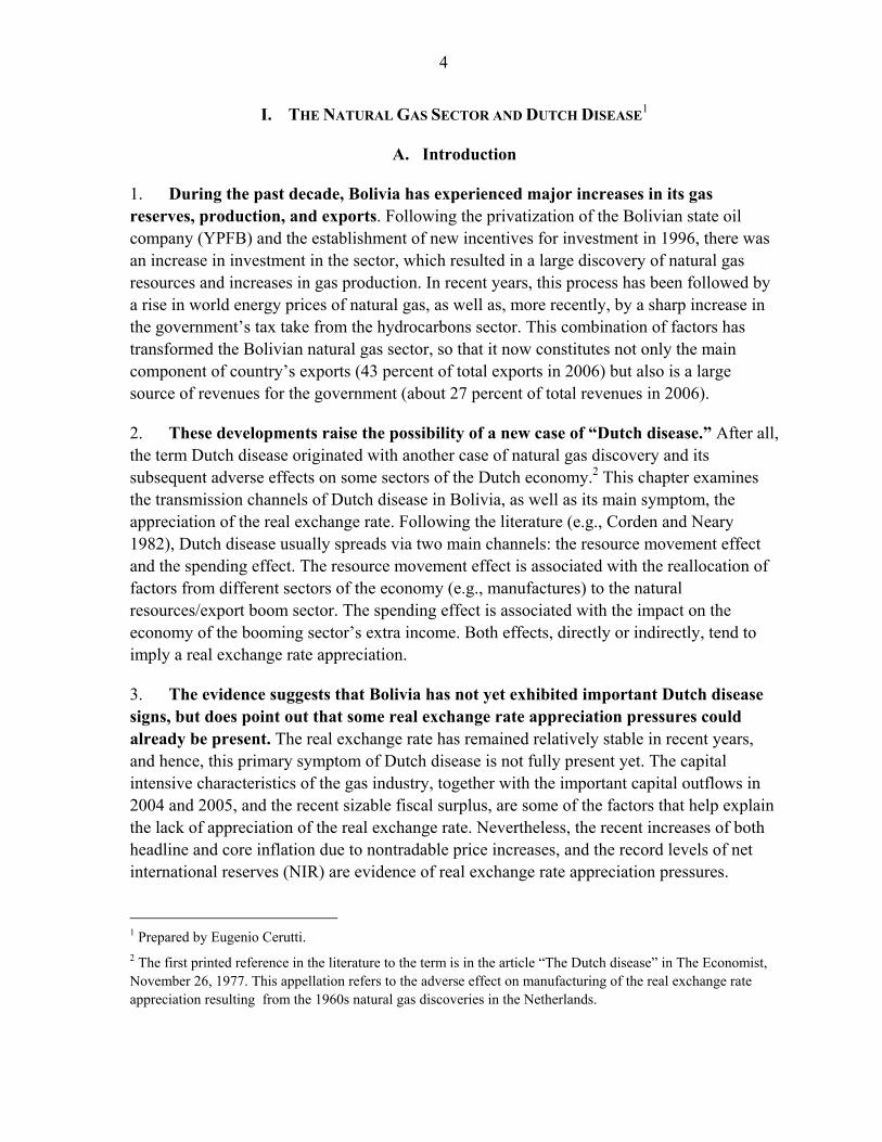
9. While Bolivia has already seen many benefits from its higher gas exports, experience elsewhere shows that effective management of natural resource wealth is key to spread the benefits more widely, contributing to improve living standards and increase potential growth. On the positive side, for example, Bolivia has reached record high NIR levels (Figure 1) in the context of a sharp turnaround in the external current account balance, from a 5 percent deficit in 2000 to an almost 12 percent surplus in 2006. Additionally, the gas sector has become one of the important sources of GDP growth. However, as discussed below, the new resources could also limit the development of other economic sectors in terms of output and factor income.
7
Figure 1. Bolivia: Macroeconomic Impact of the Gas Sector Boom
Current Account and NIR
-10
-5
0
5
10
15
1998 1999 2000 2001 2002 2003 2004 2005 20060
500
1000
1500
2000
2500
3000
3500
NIR (RHS axis, Millions of US dollars)
Current Account (% of GDP)
Real GDP Growth
-30
-20
-10
0
10
20
30
40
50
60
70
1998 1999 2000 2001 2002 2003 2004 2005 2006
GDP growth (%)Gas Sector Growth (%)
Resource movement effect
10. The economic literature identifies the ‘resource movement effect’ as the reallocation of factors from different sectors of the economy (e.g., manufactures or other lagging sectors) to the natural resources export boom sector.4 The resource movement effect is due to the increase of the marginal factor remunerations in the export boom sector. For example, if labor is mobile across production sectors, higher wages would cause a movement of labor to the export booming sector, lowering the output of the lagging sector. 5 This resource reallocation is usually called ‘direct de-industrialization’ since it does not involve appreciation of the exchange rate. However, resource reallocation can also lead to an increase in the real exchange rate as a second round effect. The relative loss of production factors in the nontradable sector would result, ex ante, in excess demand for nontradables, causing an increase in the prices of nontradables and in the real exchange rate, since the price of tradables is exogenously determined in the international markets. If more than one factor is mobile across sectors, the sign of the resource allocation effect is not clear, and it could even theoretically cause a real exchange rate depreciation (e.g., the Paradox model described by Corden and Neary 1982).
11. As is the case in most energy producers, the reallocation effect is not significant in Bolivia since the gas sector does not compete for factors with the rest of the economy. Not only does Bolivia’s hydrocarbon sector employ only around 0.04 percent of total 4 Seminal papers on this topic are Corden and Neary (1982), Corden (1984), and Sachs, J.,and A. Warner (1995). Iimi (2006) and Sala-i-Martin and Subramanian (2003) provide recent country studies. 5 In the case of Bolivia, the lagging sector can be producing both importables (e.g., agricultural sector) and/or non-boom exportables, not necessarily a manufacturing industry.
8
employment (this has not varied much since the late 1990s), but also capital movement between sectors seem to be insignificant, as the capital used in the gas industry is sector-specific and financed by FDI. In other words, there is no mobility of factors between the gas sector and the rest of the economy. In the Dutch disease literature, a sector with these characteristics is usually denominated as an “enclave” sector, as in the case of oil sectors (Corden 1984).
Spending effect
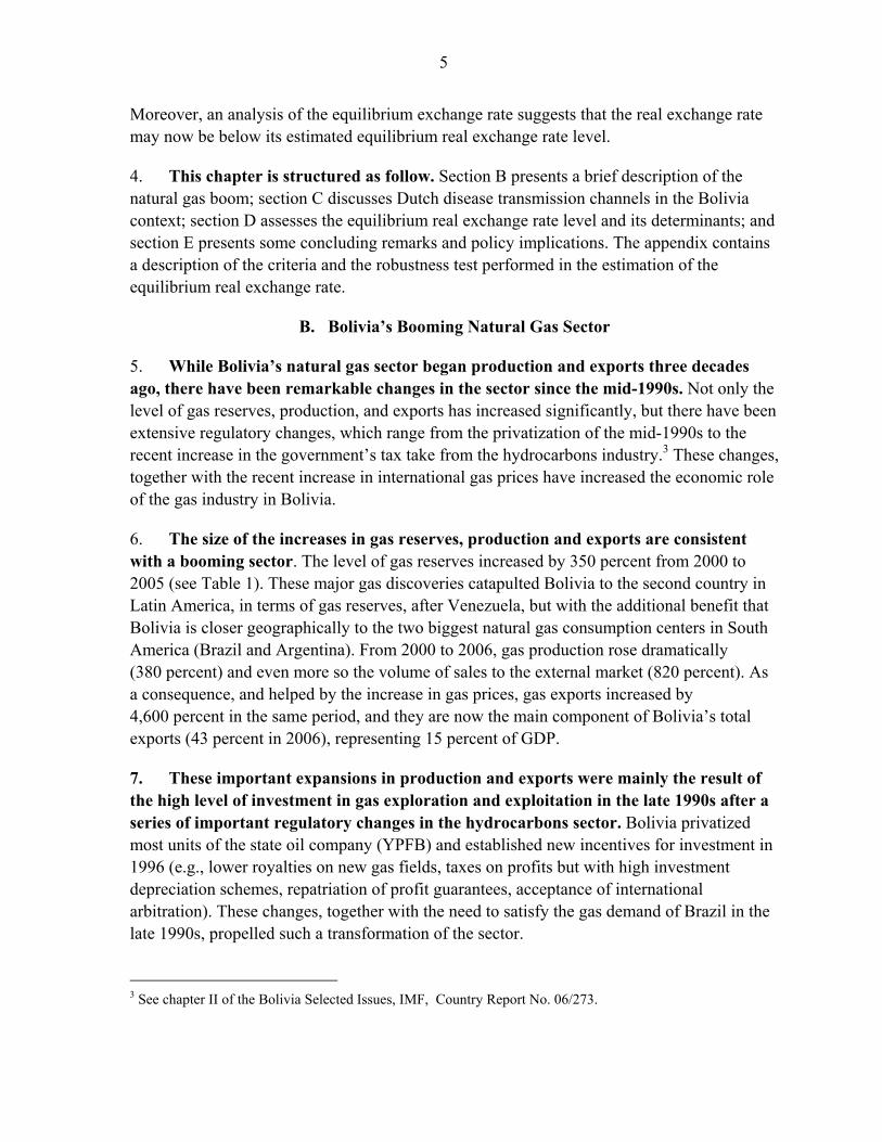
12. The spending effect relates to the appreciation of the real exchange rate as a result of the spending of some part of the booming sector’s extra income in nontradables. The spending can be performed directly by the owners of the factors of production or indirectly by the government through tax collection. The identification of the sector which carries out most of the spending is essential to determining the strength of the spending effect. The propensity to consume nontradable goods and services is usually higher in the case of the government. In general, the spending effect entails an unambiguous exchange rate appreciation, and the size of this appreciation is a function of the amount of extra resources spent in the nontradable sector.
13. Even though gas export receipts have increased and their distribution has changed towards the government, the size of the spending effect so far in Bolivia is not clear, because of the emergence of a large fiscal surplus. Following the May 2005 Hydrocarbons law and a related decree in May 2006, the participation of the government in external gas receipts increased to about 60 percent of total receipts in 2006. However, the fiscal position shifted, over this period, from an overall deficit of 9 percent of GDP in 2002 to a surplus of 4½ percent of GDP in 2006—or from a non-hydrocarbons deficit of 11 percent of GDP to a deficit of 6½ percent of GDP over the same period (Figure 2). Moreover, even though total public spending increased about 7 percent in real terms, driven by capital expenditure increases, current expenditure decreased by 6 percent in real adjusted terms.
9
Figure 2: Gas Export Receipts and the Fiscal Accounts
Distribution of Gas Exports(In millions of US dollars)
136 167452
1023
245452
634
713
102163
0
400
800
1200
1600
2000
2002 2003 2004 2005 2006
Companies' income from gas exportsGoverment take from gas exports
Fiscal Balances(In percent of GDP)
-12
-10
-8
-6
-4
-2
0
2
4
6
2002 2003 2004 2005 2006
Overall balanceNon-hydrocarbons balance
Evolution of the real exchange rate
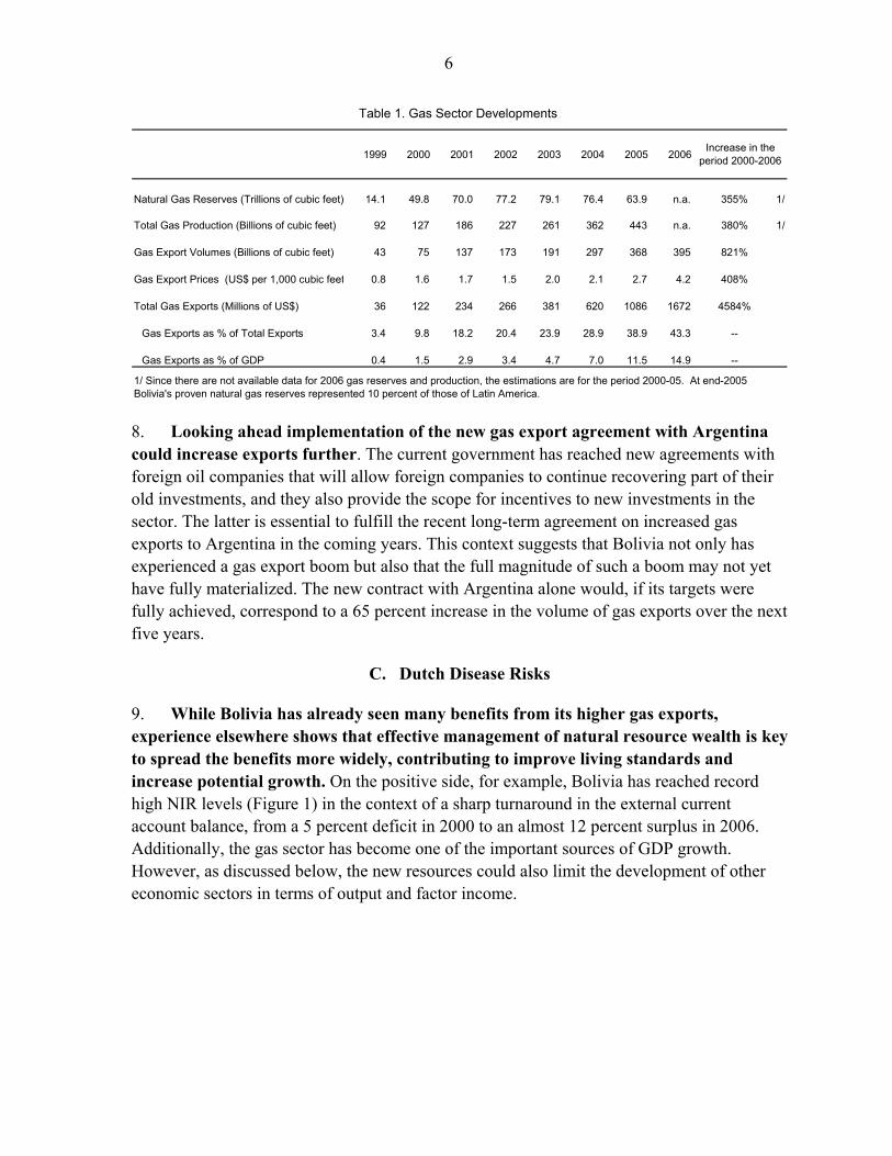
14. The CPI-based real effective exchange rate (REER) has not appreciated in recent years. 6 It displayed a downward trend from 2000 to mid-2005, and a flat trend over the last two years (Figure 3). Changes in the REER have been mostly associated with changes in the nominal effective exchange rate as the inflation rate in Bolivia has been in the single digits since 1997, and very similar to the weighted average inflation of its trading partners. The bilateral real exchange rate with the U.S. dollar exhibited similar behavior during the sample period.
15. While the behavior of the real exchange rate might seem puzzling given the gas export boom, it seems consistent with the above-described Dutch disease transmission channels. The depreciating trend through 2005 stemmed from still low prices of gas and share of government in gas export receipts, the very capital intensive nature of the gas sector, as well as from large net capital outflows (due to capital outflows related to the political crises in that period and depressed FDI). These factors seem to have been strong enough to more than offset the real exchange rate appreciation pressures from the increase in gas export volumes. In 2006, there was a reduction in capital outflows but this was partially offset by the large increase in public savings—more than half of the increase in international reserves was sterilized by an increase in government deposits. The fact that the government saved most of the extra resources from the gas sector meant that the spending effect was not set in motion.
6 See appendix A for a more detail description of the real effective exchange rate used in this note.
10
Figure 3: Real and Nominal Exchange Rate(Increase = appreciation)
50
75
100
125
150
Mar
-90
Mar
-91
Mar
-92
Mar
-93
Mar
-94
Mar
-95
Mar
-96
Mar
-97
Mar
-98
Mar
-99
Mar
-00
Mar
-01
Mar
-02
Mar
-03
Mar
-04
Mar
-05
Mar
-06
0.00
0.05
0.10
0.15
0.20
0.25
0.30
0.35
REER (2000=100)Bilateral Real Exchange Rate w ith US (2000=100)Nominal Exchange Rate (RHS, US dollar per Boliv.)
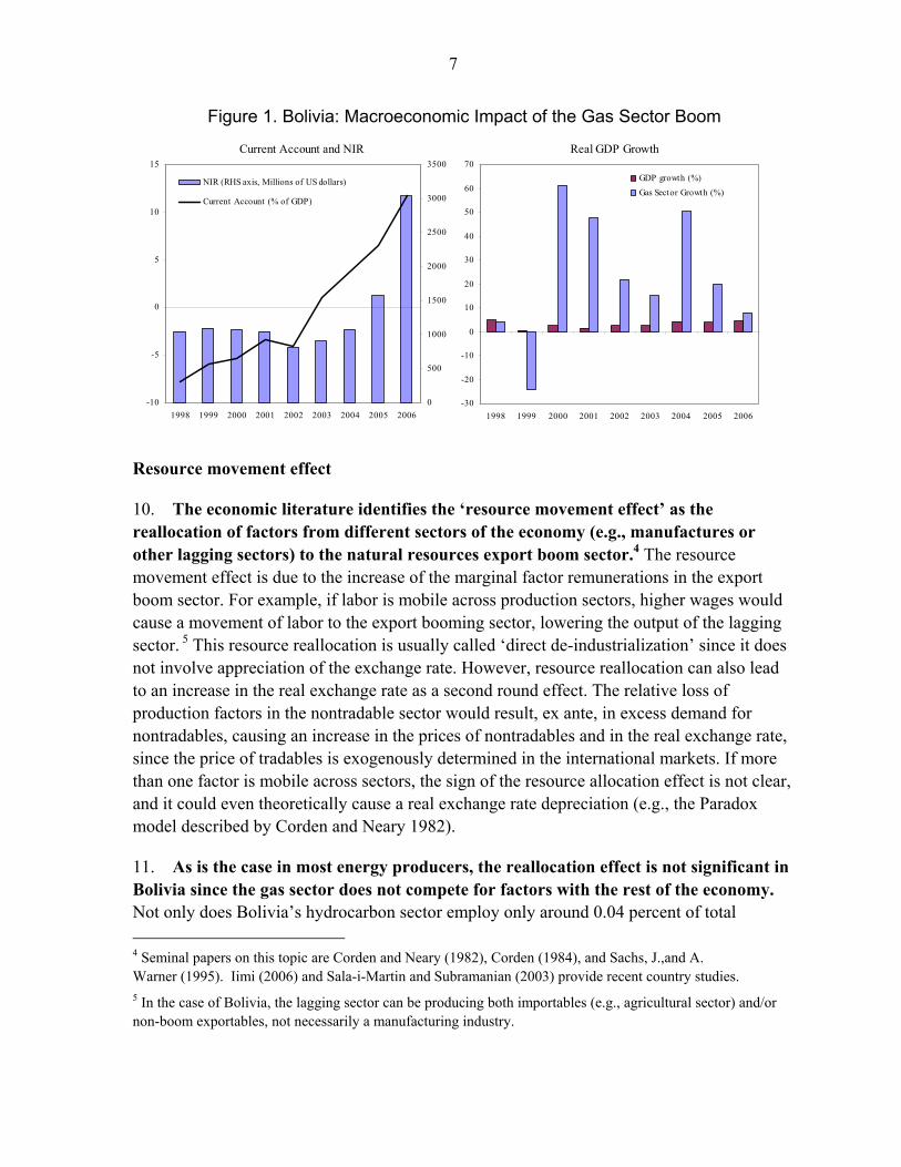
16. Nonetheless, there have been some signals of appreciation pressures in Bolivia in the more recent period. Although the nominal appreciation of the exchange rate has been relatively small, the change of the direction of the crawling peg reflects appreciation pressures. Moreover, the trend in both headline and core inflation has shifted upwards since mid-2006, with inflation of nontradables driving the change (Figure 4).
Figure 4: Quarterly Inflation in Bolivia during the Period 2000q1-2007q1
Headline and Core Inflation(in percent, annual basis)
-2-1012345678
Mar
-00
Mar
-01
Mar
-02
Mar
-03
Mar
-04
Mar
-05
Mar
-06
Mar
-07
Tradable and Non-tradable Inflation(in percent, annual basis)
-2-1012345678
Mar
-00
Mar
-01
Mar
-02
Mar
-03
Mar
-04
Mar
-05
Mar
-06
Mar
-07
Headline inflation
Core inflation Non-tradable goods inflation
Tradable goods inflation
D. Equilibrium Real Exchange Rate
17. An analysis of the equilibrium exchange rate and its determinants facilitates a better understanding of the absence thus far of significant real appreciation. This is especially relevant for the more recent period since limited exchange rate flexibility under the crawling peg regime could be masking appreciation pressures. Drawing on the recent
11
literature, in which co-integration techniques are used to identify persistent patterns of co-movements among the equilibrium exchange rate and its determinants, this section estimates a time-varying equilibrium real exchange rate by estimating a vector error correction (VEC) model, through Johansen’s (1995) maximum likelihood estimator. The advantage of this procedure is not only that it enables study of the determinants but also that it offers the possibility of measuring the equilibrium real exchange rate level and of quantifying the gap between equilibrium real exchange rate and the prevailing REER.7
Determinants of the equilibrium real exchange rate
18. Based on the main REER determinants identified in the literature for developing countries, specific variables have been selected as factors that are likely to be significant for Bolivia’s real exchange rate. These are terms of trade movements, productivity differentials vis-à-vis trading-partner countries, the size of the fiscal balance, and net capital inflows.8
• Terms of trade. An improvement in the terms of trade tends to require an appreciation of the REER in order to compensate for the positive impact on the external accounts. For example, the recent increase in commodity prices tends to raise the disposable income in Bolivia’s natural resource sectors and to increase the government’s resource envelope, both of which would put pressure on the relative prices of nontradable goods, thus offsetting the initial positive terms of trade shock.
• Productivity. An increase in productivity in the tradable sector vis-à-vis its trading partners would appreciate the REER through the well-known Balassa-Samuelson effect. The higher wages in the tradable sector due to the higher productivity would put upward pressure on wages in the nontradable sector, resulting—in the absence of nominal exchange rate adjustments—in an increase in the CPI relative to its partners. Given the lack of data on productivity for Bolivia and some of its main trading partners, the relative GDP per capita is used as a proxy for the Balassa-Samuelson effect.
7 See Hinkle and Montiel (1999) for a description of the possible determinants of the equilibrium real exchange rate. A similar VEC procedure has been applied to a number of countries, including South Africa (MacDonald and Ricci 2003), Malawi (Mathisen 2003), Algeria (Koranchelian 2005), Venezuela (Zalzuendo 2006), Jordan (Saadi-Sedik and Petri 2006), and Brazil (Paiva 2006). 8 A measure of trade openness (defined as ratio of imports plus exports over GDP) was initially included but then dropped because the increase in export and imports in recent years in Bolivia was not necessarily associated with more competition in the tradable sector. The exclusion of this variable does not affect the results presented in this chapter.
12
• Fiscal balance. The effect of this variable on the REER is ambiguous. On the one hand, an improvement in the fiscal balance would normally be accompanied by a smaller decline in private savings, reducing total domestic demand and hence increasing overall national savings. Hence, the REER would tend to depreciate since part of the decrease in domestic demand would be for nontradable goods. On the other hand, an improvement in the fiscal balance could imply an appreciation of the REER if the tightening of fiscal policy had a medium-term expansionary impact—for example, higher private investment in response to the policy credibility gain.9
• Capital inflows. Capital inflows could lead to a REER appreciation through their effect on the nontradable sector, and are approximated in this analysis by net FDI flows. Net FDI is a very important variable in Bolivia, and has ranged from 12 percent of GDP in 1999 to negative 3 percent of GDP in 2005, when a large proportion of the gas export profits was repatriated by foreign companies. The expected relationship is positive—an increase in net FDI would lead to appreciation pressures.
• Net foreign assets. The literature usually also calls for including net foreign assets in order to capture another dimension of capital flows. Economies with high levels of net foreign assets could temporally sustain a more appreciated REER because they can finance the associated trade deficits. Conversely, debtor countries might need more depreciated exchange rates in order to generate trade surpluses needed to service external liabilities. Here, the net foreign asset position of the economy is proxied by the net foreign assets of the banking system (i.e., including the central bank).
Econometric approach
19. Johansen (1995)’s maximum likelihood estimation procedure is used to identify the characteristics of the potential long run relationship between the REER and the variables discussed above. The Johansen methodology, which corrects for autocorrelation and endogeneity parametrically, can be represented in the following VEC form:
tt
p
iitit xxx εαβη ++ΔΦ+=Δ −
−
=−∑ 1
'1
1
where η is a vector of deterministic variables, ε is a vector of white noise disturbances,
1'
−txβ summarizes the long-run relationships, and α and Φ include the short-tem movements.
9 Mathisen (2003) finds this later effect significant for the case of Malawi.

13
20. Figure 5 shows the evolution of the variables under consideration, which are nonstationary in levels but stationary in first differences. The REER, terms of trade and productivity are introduced in logs, the remaining variables as percentage of GDP. The definition of the variables can be found in Appendix A, together with the Augmented Dickey-Fuller unit tests that suggest that the series are I(1), a necessary condition for applying a VEC model.
Estimation results
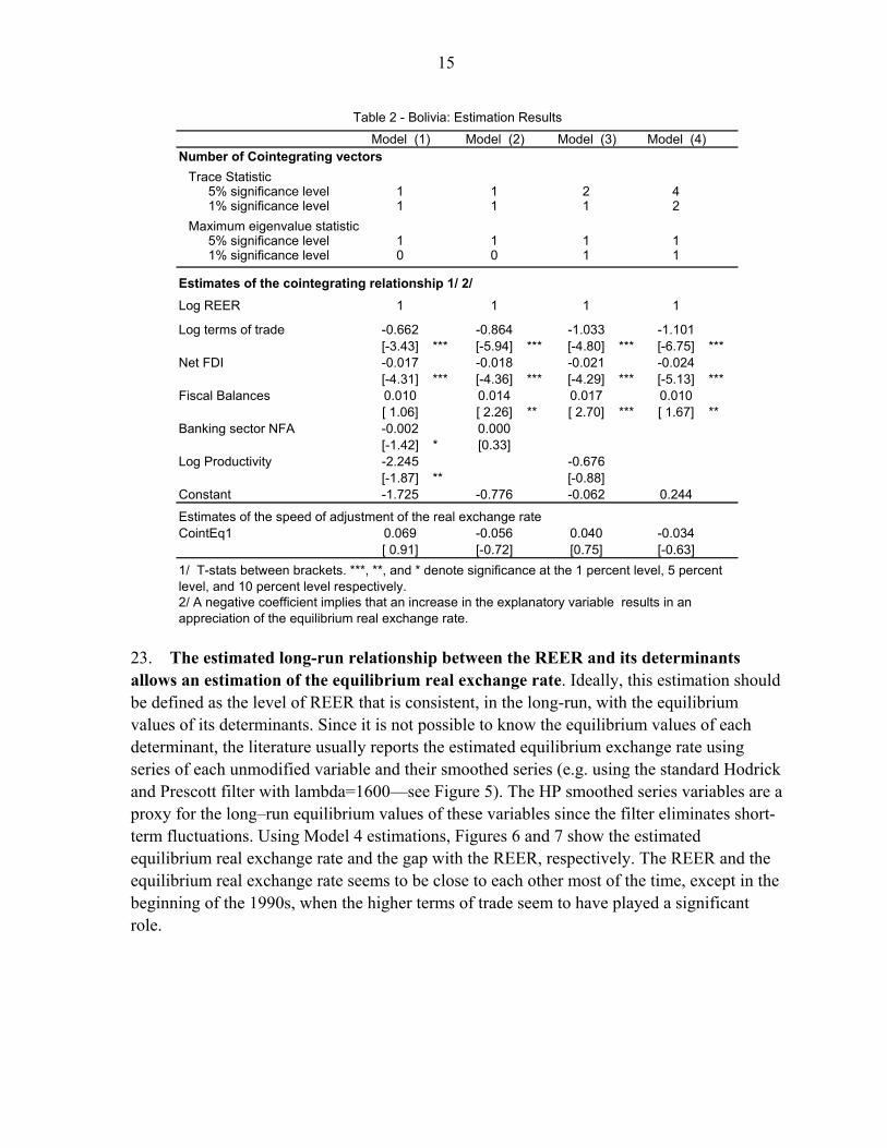
21. The estimated variables have the expected sign and there is evidence of cointegration between the REER and its determinants (Table 2). Given the standard normalization of the real exchange rate coefficient to one, a negative coefficient implies that an increase in the explanatory variable results in an appreciation of the equilibrium real exchange rate. The coefficients of the cointegrating vector (long-run relationship) have the expected sign, and in most cases, they are significant across models with the exception of two variables—productivity and banking system net foreign assets. Although these two variables are significant in model 1, their significance and stability is not uniform across models.10 With the exception of models 1 and 2, both the trace test and the maximum eigenvalue test show evidence of at least one co-integration relationship at 1 percent level. The models reported, especially model 4, showed satisfactory properties regarding the normality and no-autocorrelation of the residuals, and the lag structure specification of the model (set at 4 lags—see Appendix B). The results suggest that:
• A 1 percent increase in the terms of trade has an effect of about 1 percentage point appreciation on the REER.
• A 1 percent increase in FDI as a percentage of GDP has an effect of a 2 percent appreciation on the REER
• A 1 percent increase in the Fiscal Balance as a proportion of GDP has a 1 percent depreciation on the REER.
10 Moreover, although the productivity variable has the correct sign, the value of this coefficient is too high in model 1. Theoretically, Balassa Samuelson effect should be around the share of nontradables in the GDP. See MacDonal and Ricci (2003).
14
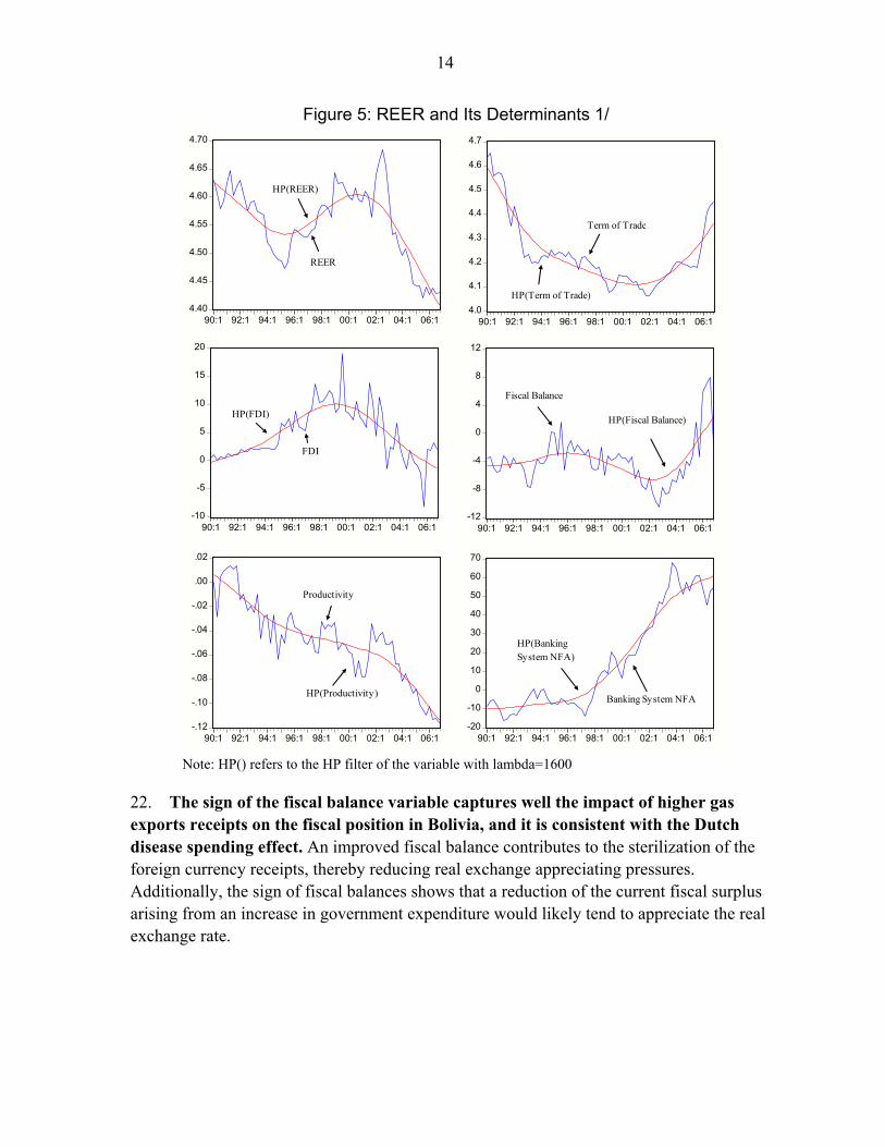
Figure 5: REER and Its Determinants 1/
4.40
4.45
4.50
4.55
4.60
4.65
4.70
90:1 92:1 94:1 96:1 98:1 00:1 02:1 04:1 06:14.0
4.1
4.2
4.3
4.4
4.5
4.6
4.7
90:1 92:1 94:1 96:1 98:1 00:1 02:1 04:1 06:1
-10
-5
0
5
10
15
20
90:1 92:1 94:1 96:1 98:1 00:1 02:1 04:1 06:1-12
-8
-4
0
4
8
12
90:1 92:1 94:1 96:1 98:1 00:1 02:1 04:1 06:1
-.12
-.10
-.08
-.06
-.04
-.02
.00
.02
90:1 92:1 94:1 96:1 98:1 00:1 02:1 04:1 06:1-20
-10
0
10
20
30
40
50
60
70
90:1 92:1 94:1 96:1 98:1 00:1 02:1 04:1 06:1
REER
HP(REER)
Term of Trade
HP(Term of Trade)
FDI
HP(FDI)
Fiscal Balance
HP(Fiscal Balance)
HP(Productivity)
Productivity
HP(Banking System NFA)
Banking System NFA
Note: HP() refers to the HP filter of the variable with lambda=1600
22. The sign of the fiscal balance variable captures well the impact of higher gas exports receipts on the fiscal position in Bolivia, and it is consistent with the Dutch disease spending effect. An improved fiscal balance contributes to the sterilization of the foreign currency receipts, thereby reducing real exchange appreciating pressures. Additionally, the sign of fiscal balances shows that a reduction of the current fiscal surplus arising from an increase in government expenditure would likely tend to appreciate the real exchange rate.
15
Number of Cointegrating vectorsTrace Statistic
5% significance level 1 1 2 41% significance level 1 1 1 2
Maximum eigenvalue statistic5% significance level 1 1 1 11% significance level 0 0 1 1
Estimates of the cointegrating relationship 1/ 2/Log REER 1 1 1 1
Log terms of trade -0.662 -0.864 -1.033 -1.101[-3.43] *** [-5.94] *** [-4.80] *** [-6.75] ***
Net FDI -0.017 -0.018 -0.021 -0.024[-4.31] *** [-4.36] *** [-4.29] *** [-5.13] ***
Fiscal Balances 0.010 0.014 0.017 0.010[ 1.06] [ 2.26] ** [ 2.70] *** [ 1.67] **
Banking sector NFA -0.002 0.000[-1.42] * [0.33]
Log Productivity -2.245 -0.676[-1.87] ** [-0.88]
Constant -1.725 -0.776 -0.062 0.244
Estimates of the speed of adjustment of the real exchange rateCointEq1 0.069 -0.056 0.040 -0.034
[ 0.91] [-0.72] [0.75] [-0.63]
Model (4)
Table 2 - Bolivia: Estimation Results
1/ T-stats between brackets. ***, **, and * denote significance at the 1 percent level, 5 percent level, and 10 percent level respectively.2/ A negative coefficient implies that an increase in the explanatory variable results in an appreciation of the equilibrium real exchange rate.
Model (1) Model (2) Model (3)
23. The estimated long-run relationship between the REER and its determinants allows an estimation of the equilibrium real exchange rate. Ideally, this estimation should be defined as the level of REER that is consistent, in the long-run, with the equilibrium values of its determinants. Since it is not possible to know the equilibrium values of each determinant, the literature usually reports the estimated equilibrium exchange rate using series of each unmodified variable and their smoothed series (e.g. using the standard Hodrick and Prescott filter with lambda=1600—see Figure 5). The HP smoothed series variables are a proxy for the long–run equilibrium values of these variables since the filter eliminates short-term fluctuations. Using Model 4 estimations, Figures 6 and 7 show the estimated equilibrium real exchange rate and the gap with the REER, respectively. The REER and the equilibrium real exchange rate seems to be close to each other most of the time, except in the beginning of the 1990s, when the higher terms of trade seem to have played a significant role.
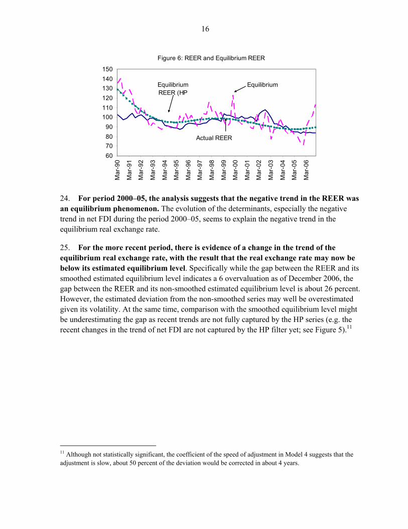
16
Figure 6: REER and Equilibrium REER
60708090
100110120130140150
Mar
-90
Mar
-91
Mar
-92
Mar
-93
Mar
-94
Mar
-95
Mar
-96
Mar
-97
Mar
-98
Mar
-99
Mar
-00
Mar
-01
Mar
-02
Mar
-03
Mar
-04
Mar
-05
Mar
-06
Equilibrium
Actual REER
Equilibrium REER (HP
24. For period 2000–05, the analysis suggests that the negative trend in the REER was an equilibrium phenomenon. The evolution of the determinants, especially the negative trend in net FDI during the period 2000–05, seems to explain the negative trend in the equilibrium real exchange rate.
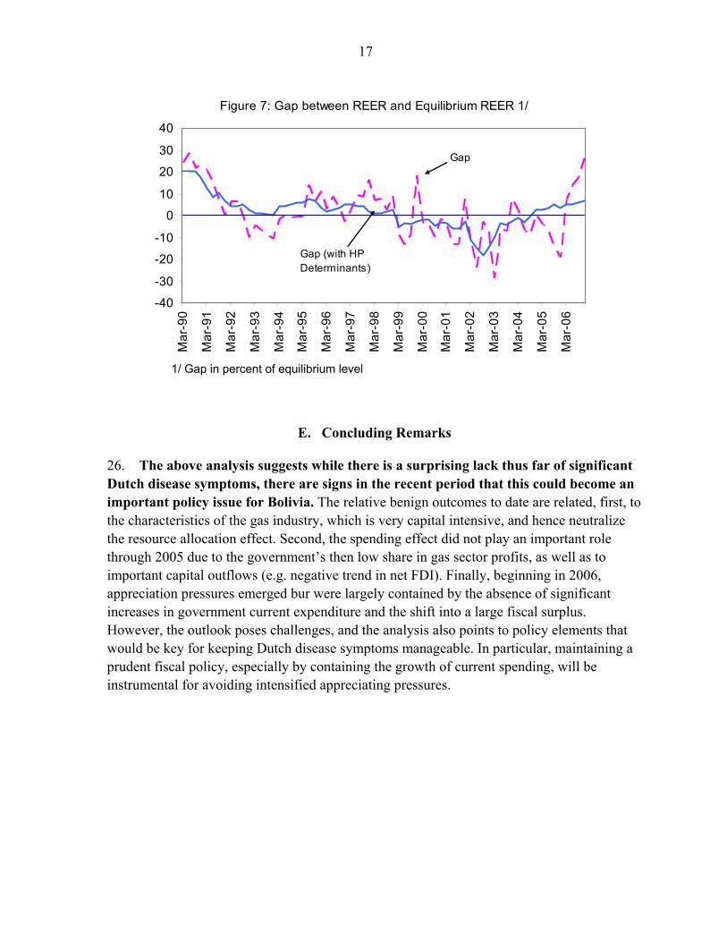
25. For the more recent period, there is evidence of a change in the trend of the equilibrium real exchange rate, with the result that the real exchange rate may now be below its estimated equilibrium level. Specifically while the gap between the REER and its smoothed estimated equilibrium level indicates a 6 overvaluation as of December 2006, the gap between the REER and its non-smoothed estimated equilibrium level is about 26 percent. However, the estimated deviation from the non-smoothed series may well be overestimated given its volatility. At the same time, comparison with the smoothed equilibrium level might be underestimating the gap as recent trends are not fully captured by the HP series (e.g. the recent changes in the trend of net FDI are not captured by the HP filter yet; see Figure 5).11
11 Although not statistically significant, the coefficient of the speed of adjustment in Model 4 suggests that the adjustment is slow, about 50 percent of the deviation would be corrected in about 4 years.
17
Figure 7: Gap between REER and Equilibrium REER 1/
-40
-30
-20
-10
0
10
20
30
40
Mar
-90
Mar
-91
Mar
-92
Mar
-93
Mar
-94
Mar
-95
Mar
-96
Mar
-97
Mar
-98
Mar
-99
Mar
-00
Mar
-01
Mar
-02
Mar
-03
Mar
-04
Mar
-05
Mar
-06
Gap
Gap (with HP Determinants)
1/ Gap in percent of equilibrium level
E. Concluding Remarks
26. The above analysis suggests while there is a surprising lack thus far of significant Dutch disease symptoms, there are signs in the recent period that this could become an important policy issue for Bolivia. The relative benign outcomes to date are related, first, to the characteristics of the gas industry, which is very capital intensive, and hence neutralize the resource allocation effect. Second, the spending effect did not play an important role through 2005 due to the government’s then low share in gas sector profits, as well as to important capital outflows (e.g. negative trend in net FDI). Finally, beginning in 2006, appreciation pressures emerged bur were largely contained by the absence of significant increases in government current expenditure and the shift into a large fiscal surplus. However, the outlook poses challenges, and the analysis also points to policy elements that would be key for keeping Dutch disease symptoms manageable. In particular, maintaining a prudent fiscal policy, especially by containing the growth of current spending, will be instrumental for avoiding intensified appreciating pressures.
18
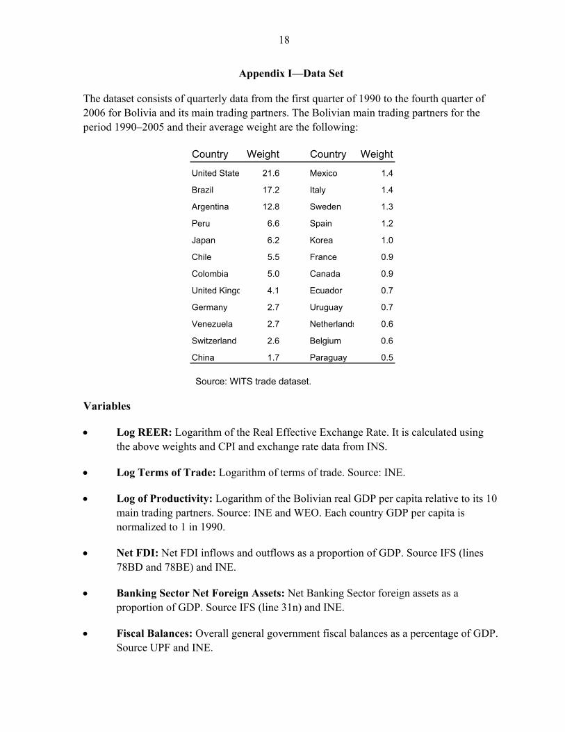
Appendix I—Data Set
The dataset consists of quarterly data from the first quarter of 1990 to the fourth quarter of 2006 for Bolivia and its main trading partners. The Bolivian main trading partners for the period 1990–2005 and their average weight are the following:
Country Weight Country Weight
United States 21.6 Mexico 1.4
Brazil 17.2 Italy 1.4
Argentina 12.8 Sweden 1.3
Peru 6.6 Spain 1.2
Japan 6.2 Korea 1.0
Chile 5.5 France 0.9
Colombia 5.0 Canada 0.9
United Kingd 4.1 Ecuador 0.7
Germany 2.7 Uruguay 0.7
Venezuela 2.7 Netherlands 0.6
Switzerland 2.6 Belgium 0.6
China 1.7 Paraguay 0.5
Source: WITS trade dataset.
Variables
• Log REER: Logarithm of the Real Effective Exchange Rate. It is calculated using the above weights and CPI and exchange rate data from INS.
• Log Terms of Trade: Logarithm of terms of trade. Source: INE.
• Log of Productivity: Logarithm of the Bolivian real GDP per capita relative to its 10 main trading partners. Source: INE and WEO. Each country GDP per capita is normalized to 1 in 1990.
• Net FDI: Net FDI inflows and outflows as a proportion of GDP. Source IFS (lines 78BD and 78BE) and INE.
• Banking Sector Net Foreign Assets: Net Banking Sector foreign assets as a proportion of GDP. Source IFS (line 31n) and INE.
• Fiscal Balances: Overall general government fiscal balances as a percentage of GDP. Source UPF and INE.
19
Appendix II—Robustness Procedures of the VEC Estimation
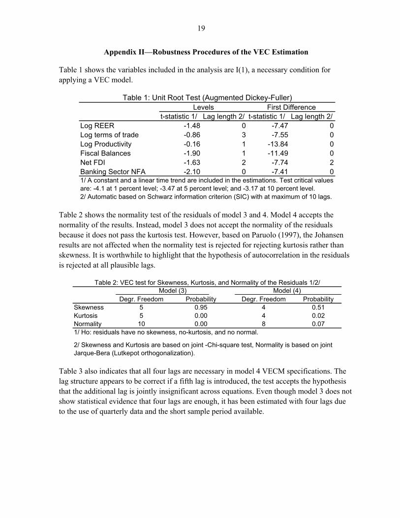
Table 1 shows the variables included in the analysis are I(1), a necessary condition for applying a VEC model.
t-statistic 1/ Lag length 2/ t-statistic 1/ Lag length 2/Log REER -1.48 0 -7.47 0Log terms of trade -0.86 3 -7.55 0Log Productivity -0.16 1 -13.84 0Fiscal Balances -1.90 1 -11.49 0Net FDI -1.63 2 -7.74 2Banking Sector NFA -2.10 0 -7.41 0
2/ Automatic based on Schwarz information criterion (SIC) with at maximum of 10 lags.
Table 1: Unit Root Test (Augmented Dickey-Fuller)Levels First Difference
1/ A constant and a linear time trend are included in the estimations. Test critical values are: -4.1 at 1 percent level; -3.47 at 5 percent level; and -3.17 at 10 percent level.
Table 2 shows the normality test of the residuals of model 3 and 4. Model 4 accepts the normality of the results. Instead, model 3 does not accept the normality of the residuals because it does not pass the kurtosis test. However, based on Paruolo (1997), the Johansen results are not affected when the normality test is rejected for rejecting kurtosis rather than skewness. It is worthwhile to highlight that the hypothesis of autocorrelation in the residuals is rejected at all plausible lags.
Degr. Freedom Probability Degr. Freedom ProbabilitySkewness 5 0.95 4 0.51Kurtosis 5 0.00 4 0.02Normality 10 0.00 8 0.071/ Ho: residuals have no skewness, no-kurtosis, and no normal.
Model (3) Model (4)
2/ Skewness and Kurtosis are based on joint -Chi-square test, Normality is based on joint Jarque-Bera (Lutkepot orthogonalization).
Table 2: VEC test for Skewness, Kurtosis, and Normality of the Residuals 1/2/
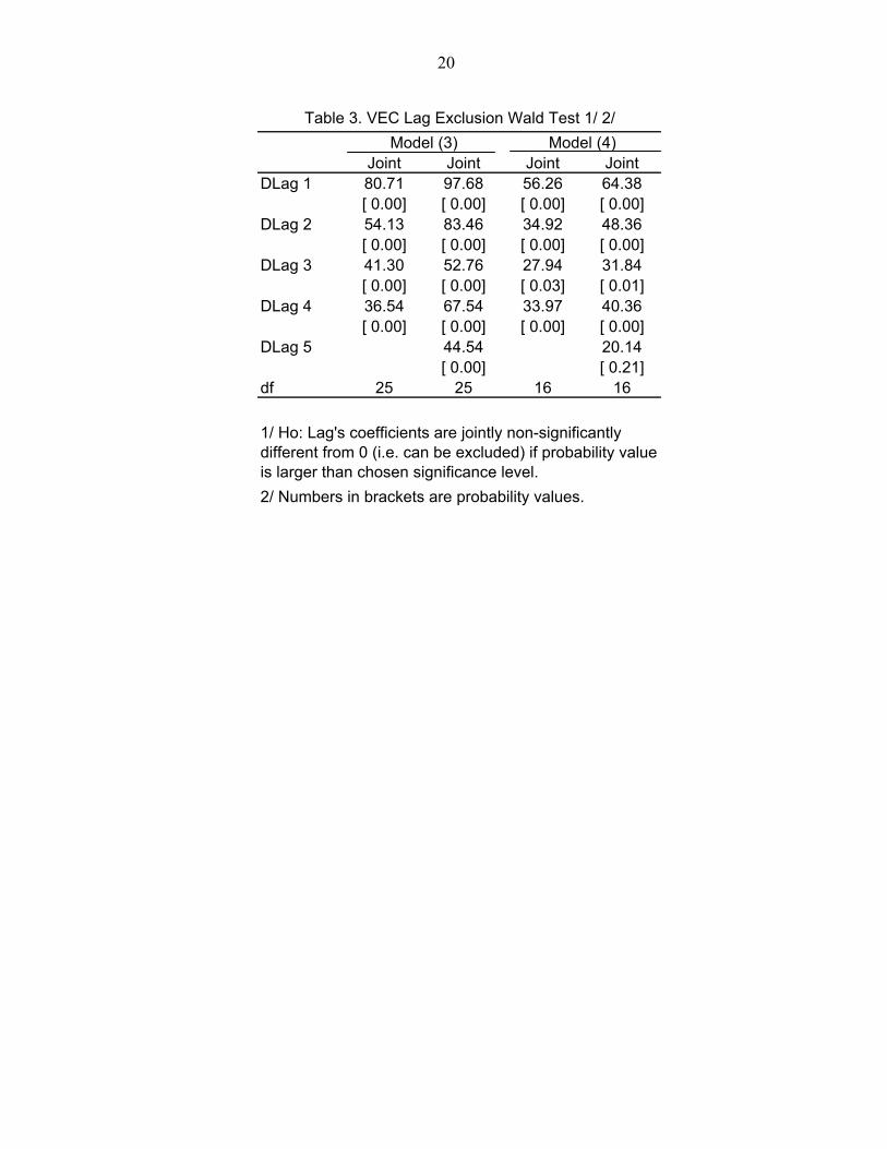
Table 3 also indicates that all four lags are necessary in model 4 VECM specifications. The lag structure appears to be correct if a fifth lag is introduced, the test accepts the hypothesis that the additional lag is jointly insignificant across equations. Even though model 3 does not show statistical evidence that four lags are enough, it has been estimated with four lags due to the use of quarterly data and the short sample period available.
20
Joint Joint Joint JointDLag 1 80.71 97.68 56.26 64.38
[ 0.00] [ 0.00] [ 0.00] [ 0.00]DLag 2 54.13 83.46 34.92 48.36
[ 0.00] [ 0.00] [ 0.00] [ 0.00]DLag 3 41.30 52.76 27.94 31.84
[ 0.00] [ 0.00] [ 0.03] [ 0.01]DLag 4 36.54 67.54 33.97 40.36
[ 0.00] [ 0.00] [ 0.00] [ 0.00]DLag 5 44.54 20.14
[ 0.00] [ 0.21]df 25 25 16 16
2/ Numbers in brackets are probability values.
Table 3. VEC Lag Exclusion Wald Test 1/ 2/Model (3) Model (4)
1/ Ho: Lag's coefficients are jointly non-significantly different from 0 (i.e. can be excluded) if probability value is larger than chosen significance level.
21
References
Clark, P., and R. MacDonald, 1998, “Exchange Rate and Economic Fundamentals: A Methodology Comparison of BEERs and FEERs,” IMF Working Paper 98/67 (Washington: International Monetary Fund).
Corden, M., 1984, “Booming Sector and Dutch Disease Economics: Survey and Consolidation,” Oxford Economic Papers, Vol. 36 (November), pp. 359–80.
––––––, and P. Neary 1982, “Booming Sector and De-Industrialization in a Small Open Economy,” The Economic Journal, Vol. 92 (December), pp. 825–48.
Hamilton, J., 1994, “Time Series Analysis,” Princeton, NJ, Princeton University Press.
Hinkle, L. and P. Montiel, 1999, “Exchange Rates Misalignments: Concepts and Measurements for Development Countries,” Oxford University Press.
Iimi, Atsushi, 2006. “Did Botswana Scape the Resource Curse”. IMF Working Paper 06/138 (Washington: International Monetary Fund).
International Monetary Fund, 2006, “Bolivia, Selected Issues Papers,” IMF Staff Country Report 06/273 (Washington: International Monetary Fund).
MacDonald, R., and L. Ricci, 2003, “Estimation of the Equilibrium Real Exchange Rate for South Africa,” IMF Working Paper 03/44 (Washington: International Monetary Fund).
Paiva, C.,2006, “External Adjustment and Equilibrium Exchange Rate in Brazil,” IMF Working Paper 06/221 (Washington: International Monetary Fund).
Paruolo, P., 1997, “Asymptotic Inference on the Moving Average Impact Matrix in Co-Integrated I(1) VAR System,” Econometric Theory, Vol. 13, pp 79–118.
Saadi-Sedik, T., and M. Petri, 2006, “To Smooth or Not to Smooth-The Impact of Grants and Remittances on the Equilibrium Real Exchange Rate in Jordan,” IMF Working Paper 06/257 (Washington: International Monetary Fund).
Sachs, J., and A. Warner, 1995, “Natural Resource Abundance and Economic Growth,” NBER Working Paper 5398 (Cambridge, Massachusetts: National Bureau of Economic Research).
Sala-i-Martin, Xavier and Arvind Subramanian, 2003. “Addressing the Natural Resource Curse: An Illustration from Nigeria”. IMF Working Paper 03/139 (Washington: International Monetary Fund)
22
Target Consulting Group, 2004, “International Hydrocarbons Fiscal Systems Benchmarking Review,” Report for the U.S. Agency for International Development. Available at http://pdf.usaid.gov/pdf_docs/PNADC391.pdf
World Bank, 2006, “Por el Bienestar de Todos, Bolivia,” (Washington, D.C.).
Zalduendo, J., 2006, “Determinants of Venezuela’s Equilibrium Exchange Rate,” IMF Working Paper 06/74 (Washington: International Monetary Fund).
23
II. TAX SYSTEM: STRUCTURE AND REFORM OPTIONS1
A. Introduction
1. In recent years Bolivia experienced a marked increase in revenue collection mostly due to a large increase in hydrocarbon royalties. The favorable external environment, reflected in a more than doubling in natural gas export prices, and a change in the tax take, which more than doubled the level of royalties, are the main factors underlying an increase in hydrocarbon royalties by about 8 percentage points of GDP in the period 2003–06.2 Revenues from regular taxation3 also increased in the same period, by about 4 percentage points of GDP, reflecting higher growth, improved corporate income tax collections from the hydrocarbons sector, the impact of tax administration reforms, and improvements in taxpayer compliance. These revenue developments, coupled with slow growth of spending, resulted in a large shift in the overall fiscal balance—from a deficit of about 8 percent of GDP in 2003 to a surplus of about 5 percent of GDP in 2006.
2. The drastic change in the fiscal situation provides a good opportunity to review the tax system with a focus on strengthening its capacity to collect revenues efficiently and equitably. In the period 2001–04, the high fiscal deficits were driven by large increases in spending related to social tensions, which were not accompanied by increases in revenue. The concerns created by the high deficit and the difficulties in adjusting spending, led to the adoption of stop-gap tax policy measures (such as the introduction of a financial transactions tax), with a clear loss in terms of efficiency and equity. The strengthening in the fiscal position provides a chance to analyze the tax system with a focus on these two key dimensions, and to consider reform options.
3. This chapter reviews the main elements of Bolivia’s tax system and discusses options to improve its efficiency and equity. It focuses on the main national taxes4 and special regimes and is divided in four sections. Section B describes the main groups of taxes forming the Bolivian tax system, recent developments in the level and composition of revenues and recent modifications to the system. Section C discusses main issues related to each group of taxes and special regimes. Section D discusses reform options.
1 Prepared by Alejandro Simone. 2 Royalties were increased in 2005, from 18 percent to 50 percent of the production value. An additional temporary royalty of 32 percent on the production of the two largest gas fields for the national oil company YPFB was established in the May 2006 nationalization decree, and lasted until April 2007. 3 Revenues from regular taxation exclude royalties and revenue from tax amnesties. 4 The paper does not cover issues related to trade taxes, sub national taxation and the sector-specific hydrocarbon and mining taxation regimes.
24
B. Tax System: Structure and Recent Developments5
4. Bolivia has a relatively simple tax system, based mainly on consumption taxes (Table 1). These include the value added tax (VAT), a transactions tax (IT), a financial transactions tax (ITF), and two types of excise taxes—excise taxes on beverages, tobacco, and vehicles (ICE); and excise taxes on hydrocarbons and its derivative products (IEHD). Revenue from these taxes averaged about 11 percent of GDP, and represented on average about 57 percent of tax revenue6 in the period 2001–06.
5. In recent years the composition of tax revenue has been changing and the importance of royalties has increased sharply. In addition to the large increases in prices of gas and tax take from hydrocarbons, mining royalties have also boomed due to high international prices. Since 2003, the share of royalties in tax revenue has more than doubled, reaching 37½ percent in 2006. Similarly, the overall contribution of the hydrocarbon sector to tax revenue (which includes corporate income tax payments by the sector) has risen by about 20 percentage points, to over 50 percent in 2006.
6. The other main components of the tax system include taxes on income and profit, custom duties, subnational property taxes, and special regimes for small taxpayers and for certain regions. While Bolivia does not have a personal income tax, it has RC-IVA, a tax mostly on wages and interest income whose revenue, has been gradually declining, and a corporate income tax (IUE), which, in contrast, has been showing some improvement in collections. Regarding special regimes, these apply to small taxpayers in trade (RTS), transport (RTI), and agriculture (RAU), whose revenues have been negligible. The special regimes for regions include free trade zones and a set of special tax exemptions.
7. Following the adoption of the current tax code in 2003, and the introduction of a financial transactions tax in 2004, the changes in the tax system were mainly in hydrocarbons, with only modest changes in other areas. In 2005, a new direct tax on hydrocarbons (IDH) was introduced, implying a de facto increase in the royalty level, from 18 percent to 50 percent. Also, IEHD excises on diesel and gasoline were increased. In 2006, there was a reduction in the rate of the financial transactions tax, from 0.25 percent to 0.15 percent, along with a narrowing of the definition of its base to cover only transactions in foreign currency. In addition, passenger transportation services between regional departments were moved from the RTI special regime into the regular regime.
5 Appendix I provides a more detailed description of the Bolivian tax system. 6 Unless indicated otherwise, “tax revenue” refers to the total tax revenue of the general government.
25
C. Key Tax Policy Issues
8. This section discusses issues that should be addressed concerning the three main groups of taxes covered in this chapter. The first part discusses issues with taxes on income and profits, the second part discusses issues regarding taxes on goods and services, and the third part discusses issues related to the special regimes for small taxpayers and the special regimes for certain regions.
Taxes on profit and income
9. The complementary tax to VAT (RC-IVA). The RC-IVA was designed to strengthen control over sales of retailers to the final consumers. However, the presentation of fraudulent invoices or sale of invoices from taxpayers with excess credits in a secondary market, have become difficult and administratively costly to control. This has resulted in a continued decline in revenue. Moreover, the associated liability is an increasing function of savings, which provides an incentive to increase consumption. More fundamentally, the RC-IVA is effectively a narrow base version of a personal income tax. The tax base is made up of only a few types of income and given the problem with invoices, most of the collections come from interest withholding (which is final) and concentrates the burden on taxpayers with this type of income. In addition, it does not provide the kind of progressivity to the tax system that a more general personal income tax with a progressive rate schedule would.
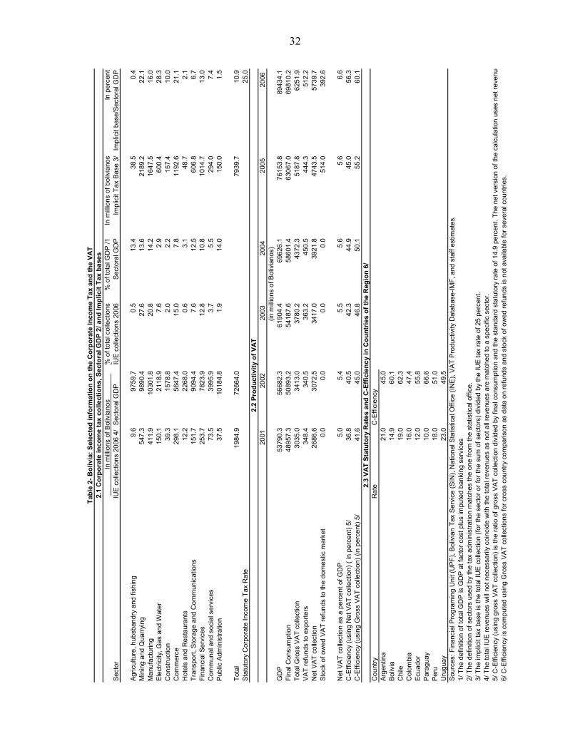
10. The corporate income tax (IUE). While the tax base of the IUE has grown with respect to previous estimations, there is evidence that it remains significantly below its potential. Table 2 compares the share of revenues obtained from a sector in total IUE collections with its share in GDP and computes implicit IUE tax bases for each sector and for IUE as a whole. The share of certain sectors (e.g. agriculture and hotels/restaurants) in total IUE collections is well below their share in GDP. Moreover, the implied IUE tax base is only about 11 percent of the GDP generated in the different sectors while the statutory corporate income tax rate is 25 percent. The relatively small size of the tax base relative to its potential is likely to be related to several mechanisms of tax avoidance that are not adequately addressed in the legislation. These include, among others: (a) transfer pricing: subsidiaries selling their output at artificially low prices to shift their profits to a country with lower tax burden (b) thin capitalization (companies have artificial incentives to borrow either from banks or related companies to inflate the interest bill that is tax deductible); (c) exemptions, such as for companies operating in certain free trade zones, and for capital gains from assets registered in the stock market; and (d) generous loss carry over provisions. In addition, the fact that only profits generated in Bolivia are part of the tax base reduces incentives for domestic investment.
26
Taxes on goods and services
11. The transactions tax (IT). In its current form, the IT is acting as a de facto minimum profit tax and is an important source of revenue. The base of the tax is essentially gross income or sales and the payment of the IUE can be deducted for the computation of the tax liability of the IT, characteristics that are similar to the ones a minimum profit tax on turnover. However, the tax generates several distortions. First, it is a “cascading” tax, i.e., it penalizes businesses that have many stages of production, thereby providing distortionary incentives to vertical integration. Second, it penalizes domestic production as importers are not subject to the tax. Finally, exporters typically cannot get a refund for the IT on their inputs, which artificially makes them less competitive.
12. The financial transactions tax (ITF). The financial transactions tax was created in 2004, in a context of emergency revenue need, for an initial period of two years. The tax rate was initially set at 0.30 percent for both credits and debits, and then reduced to 0.25 percent in 2005. In 2006, the ITF was made permanent, its rate was reduced further to 0.15 percent, and transactions in bolivianos were exempted as part of the government’s strategy to reduce dollarization. While the ITF provided needed revenues in a crisis situation, its costs may outweigh its benefits given the improved fiscal position. In particular, it increases the costs of financial intermediation, a large share of which remains denominated in U.S. dollars.
13. The value added tax (VAT). The VAT is in general a well designed tax and its efficiency has improved in recent years. Its productivity, as measured by the C-efficiency coefficient has been growing, and there has been an important increase in collection levels as a share of GDP7 (Table 2). This is likely to reflect a combination of a stronger level of economic activity and an improvement in tax administration. Some aspects, however, could be strengthened. First, excise taxes are not included in the base of the VAT, which runs against the externality correction function of excises. Second, fraudulent invoicing has contributed to the setting of discretionary limits to the amount of refunds that can be paid to certain sectors, leading to an accumulation of unpaid refunds to some exporters. Finally, the regulation of the tax does not clearly define what constitutes an export of a service.
14. Excise taxes (ICE and IEHD). Although the introduction of tax amnesties has been avoided in the last two years, the repeated use of such amnesties in the past eroded the base of the ICE. In particular, tax amnesties on imported vehicles as a source of revenue in the crisis years has contributes to a continued expectation of future amnesties. In addition to evasion problems with vehicles, some studies provided evidence of significant evasion in the collection of excises on tobacco and beverages. Regarding the IEHD, the administrative nature of the adjustment of rates, coupled with incentives to use IEHD rates to keep domestic 7 The level of C-efficiency compares favorably with other countries in the region (Table 2), which is in part due to the fact that the Bolivian VAT has one of the fewest numbers of exempted goods and services.
27
retail prices of hydrocarbon products low, has typically hurt IEHD revenues and hindered the externality correction role of the tax.
Special regimes for small taxpayers and regions
15. The system of special regimes for small taxpayers has several features that reduce the efficiency and equity of the tax system. First, the treatment of taxpayers on the basis of the type of activity allows taxpayers that should normally be taxed in the regular regime to obtain a preferential tax treatment by dividing up their activities (thereby favoring large taxpayers who can easily divide up their activities). Second, within the same type of activity, it favors unfair competition by informal businesses, as the latter are typically treated under the special regimes under advantageous conditions. Third, given that informality is favored, it makes tax evasion and smuggling more difficult to control, particularly for some taxes such as the VAT, given that special regime taxpayers are not allowed to issue invoices. Finally, the several categories of special regimes generate costs and difficulties for the tax administration, diverting valuable resources that could be used more efficiently to monitor larger taxpayers.
16. The special tax regimes or free trade zone is overly complex and provides numerous opportunities for tax avoidance or evasion. There are currently 14 free trade zones and several elements of legislation exempting certain regions from a specific group of taxes. While the authorities have limited the impact of these laws with the related regulation, the special concessions granted to certain regions have provided arguments to other regions to ask for similar treatment, leading to further complexity. Regarding the avoidance problem, by locating activities in a specific region, or by exploiting ambiguities in a complex legislation, certain group of taxpayers have been able to artificially reduce their tax burden. For example, some enterprises use free trade zones exemption to IUE to distribute dividends to local shareholders, and they similarly can avoid paying VAT. In addition, the fact that the tax administration is overburdened leads to a perception of low risk and provides taxpayers with significant opportunities for tax evasion. This is evidenced, for example, by the low level of taxpayer compliance in the regime covering the transportation sector, where the evasion rate reached a high of about 70 percent before some taxpayers were shifted in 2006 to the regular regime.
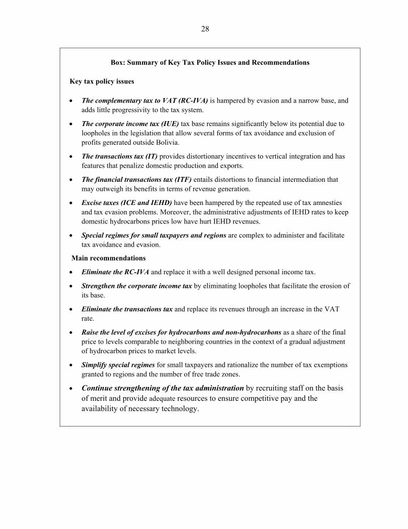
28
Box: Summary of Key Tax Policy Issues and Recommendations
Key tax policy issues • The complementary tax to VAT (RC-IVA) is hampered by evasion and a narrow base, and
adds little progressivity to the tax system.
• The corporate income tax (IUE) tax base remains significantly below its potential due to loopholes in the legislation that allow several forms of tax avoidance and exclusion of profits generated outside Bolivia.
• The transactions tax (IT) provides distortionary incentives to vertical integration and has features that penalize domestic production and exports.
• The financial transactions tax (ITF) entails distortions to financial intermediation that may outweigh its benefits in terms of revenue generation.
• Excise taxes (ICE and IEHD) have been hampered by the repeated use of tax amnesties and tax evasion problems. Moreover, the administrative adjustments of IEHD rates to keep domestic hydrocarbons prices low have hurt IEHD revenues.
• Special regimes for small taxpayers and regions are complex to administer and facilitate tax avoidance and evasion.
Main recommendations
• Eliminate the RC-IVA and replace it with a well designed personal income tax.
• Strengthen the corporate income tax by eliminating loopholes that facilitate the erosion of its base.
• Eliminate the transactions tax and replace its revenues through an increase in the VAT rate.
• Raise the level of excises for hydrocarbons and non-hydrocarbons as a share of the final price to levels comparable to neighboring countries in the context of a gradual adjustment of hydrocarbon prices to market levels.
• Simplify special regimes for small taxpayers and rationalize the number of tax exemptions granted to regions and the number of free trade zones.
• Continue strengthening of the tax administration by recruiting staff on the basis of merit and provide adequate resources to ensure competitive pay and the availability of necessary technology.
29
D. Reform Options
17. The above discussion suggests that some taxes have weak bases, high administrative costs, and a distortionary impact. The tax system has been complicated by the introduction of several special regimes for small taxpayers and particular regions that generate incentives for informality and tax evasion, and also treat differently taxpayers with potentially similar capacity to pay, depending on their characteristics such as the type of economic activity. Finally, given the important reliance on taxes on goods and services and the lack of a well functioning personal income tax , there is little progressivity in the system, an essential characteristic for vertical equity. In order to address these issues and avoid a further increase in the dependence on hydrocarbon revenues, reforms could be considered based on an appropriate combination over time of the following measures:
• Eliminating the RC-IVA and replacing it with a well designed personal income tax. A simple tax design with moderate marginal rates (e.g. between 5 and 25 percent), a high exemption threshold, standardized deductions, and a broad tax base covering all sources of income would help improve efficiency and strengthen the vertical and horizontal equity in the tax system. While the yield of the measure will ultimately depend on the exact design of the tax, a personal income tax with these characteristics could yield a gross revenue level of 1 percent of GDP. After deducting the revenue loss from the elimination of the RC-IVA and other related changes, the net revenue gain could be around 0.5 percent of GDP.
• Eliminating the transactions tax and replacing its revenues through an increase in the VAT rate. This would limit the problems related to cascading, artificial disincentives to domestic production, and reduction in competitiveness of exporters. Depending on how much the elimination of the IT would affect the base of the VAT, an increase in the gross VAT rate of between 4 and 5 points would be needed to compensate for lost revenues from the IT. Given the current rate of 13 percent, this would leave Bolivia with a VAT rate closer to those of neighboring countries (Table 2).
• Strengthening the corporate income tax by eliminating loopholes that facilitate the erosion of its base. This includes: (a) implementing guidelines on transfer pricing in line with the OECD guidelines; (b) limiting the possibilities for interest deductions, to avoid thin capitalization; (c) eliminating the exemption for capital gains from assets registered in the stock market; (d) limiting loss carry over provisions; and (e) making the tax apply to worldwide profits and not only to profits generated in Bolivia. In addition, given that the IT would not longer act as a minimum profit tax, a 1 percent minimum profit tax based on assets could be introduced temporarily, as several countries in the region have done to ensure a certain level of revenue during the
30
transition to the reformed IUE. While it is very difficult to quantify ex-ante the yield of such measures, about 0.3 percent of GDP would be a conservative estimate.
• Simplifying special regimes for small taxpayers and rationalizing the number of tax exemptions granted to regions and the number of free trade zones. The simplification of the special regime for small taxpayers could be achieved by replacing them with a unique regime for small taxpayers. Two thresholds based on turnover would be introduced—a lower threshold below which the taxpayer would be exempt from the VAT and IUE, and a higher one above which taxpayers would have to contribute to the regular regime. Taxpayers in between these thresholds would only pay the corporate income tax, on a presumptive basis. Exemptions for regions and free trade zones should be reviewed and their coverage reduced to a minimum, taking into account a quantification of their associated tax expenditures.
• Raising the level of excises for hydrocarbons and non-hydrocarbons as a share of the final price to levels comparable to neighboring countries. The former should be undertaken in the context of a gradual adjustment of hydrocarbon prices to market levels. Avoiding erosion of the level of excises as a share of the final price is important to ensure that there is adequate correction for the externalities typically generated by the consumption of the covered goods. However, and particularly in the case of the ICE, these changes will need to be accompanied by increased tax administration efforts to fight evasion and smuggling. Depending on the magnitudes of adjustment in prices and rates, this reform could generate significant additional revenue.
18. The effectiveness of the above tax policy reforms would hinge on continued improvement in tax administration. In this connection, efforts should continue to recruit staff on the basis of merit and to provide the necessary resources to the tax and customs administrations, so that these institutions can pay competitively to their staff and acquire the necessary technology to support appropriate revenue administration procedures.
Reference
Coelho, Isaias ; Ebrill, Liam P., and Victoria P. Summers, 2001, “Bank Debit Taxes in Latin
America - An Analysis of Recent Trends,” IMF Working Paper No. 01/67 (Washington: International Monetary Fund).
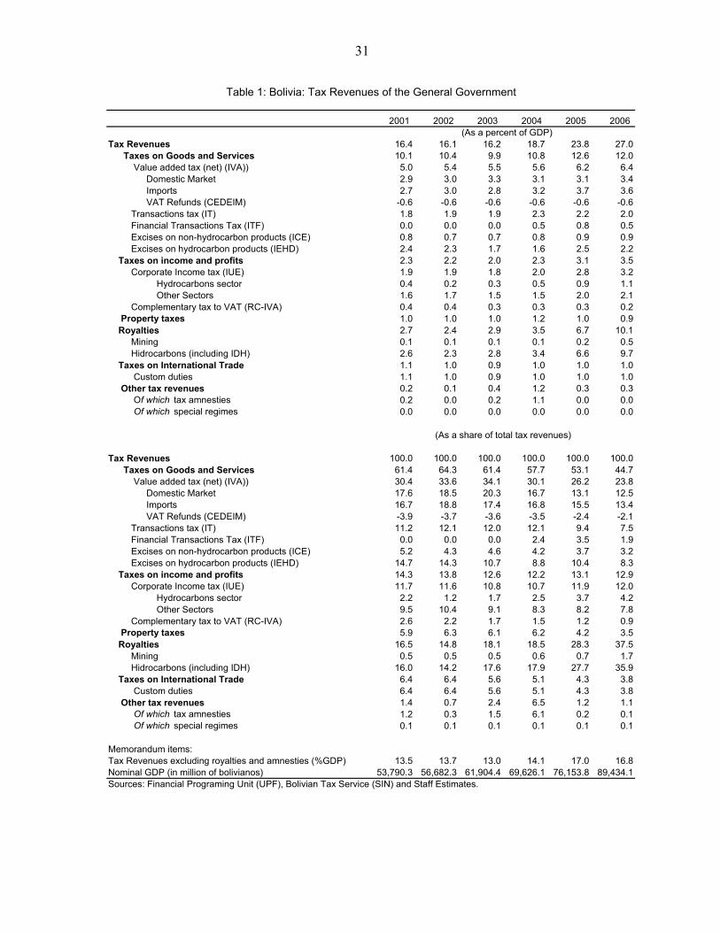
31
2001 2002 2003 2004 2005 2006
Tax Revenues 16.4 16.1 16.2 18.7 23.8 27.0 Taxes on Goods and Services 10.1 10.4 9.9 10.8 12.6 12.0 Value added tax (net) (IVA)) 5.0 5.4 5.5 5.6 6.2 6.4 Domestic Market 2.9 3.0 3.3 3.1 3.1 3.4 Imports 2.7 3.0 2.8 3.2 3.7 3.6 VAT Refunds (CEDEIM) -0.6 -0.6 -0.6 -0.6 -0.6 -0.6 Transactions tax (IT) 1.8 1.9 1.9 2.3 2.2 2.0 Financial Transactions Tax (ITF) 0.0 0.0 0.0 0.5 0.8 0.5 Excises on non-hydrocarbon products (ICE) 0.8 0.7 0.7 0.8 0.9 0.9 Excises on hydrocarbon products (IEHD) 2.4 2.3 1.7 1.6 2.5 2.2 Taxes on income and profits 2.3 2.2 2.0 2.3 3.1 3.5 Corporate Income tax (IUE) 1.9 1.9 1.8 2.0 2.8 3.2 Hydrocarbons sector 0.4 0.2 0.3 0.5 0.9 1.1 Other Sectors 1.6 1.7 1.5 1.5 2.0 2.1 Complementary tax to VAT (RC-IVA) 0.4 0.4 0.3 0.3 0.3 0.2 Property taxes 1.0 1.0 1.0 1.2 1.0 0.9 Royalties 2.7 2.4 2.9 3.5 6.7 10.1 Mining 0.1 0.1 0.1 0.1 0.2 0.5 Hidrocarbons (including IDH) 2.6 2.3 2.8 3.4 6.6 9.7 Taxes on International Trade 1.1 1.0 0.9 1.0 1.0 1.0 Custom duties 1.1 1.0 0.9 1.0 1.0 1.0 Other tax revenues 0.2 0.1 0.4 1.2 0.3 0.3 Of which tax amnesties 0.2 0.0 0.2 1.1 0.0 0.0 Of which special regimes 0.0 0.0 0.0 0.0 0.0 0.0
Tax Revenues 100.0 100.0 100.0 100.0 100.0 100.0 Taxes on Goods and Services 61.4 64.3 61.4 57.7 53.1 44.7 Value added tax (net) (IVA)) 30.4 33.6 34.1 30.1 26.2 23.8 Domestic Market 17.6 18.5 20.3 16.7 13.1 12.5 Imports 16.7 18.8 17.4 16.8 15.5 13.4 VAT Refunds (CEDEIM) -3.9 -3.7 -3.6 -3.5 -2.4 -2.1 Transactions tax (IT) 11.2 12.1 12.0 12.1 9.4 7.5 Financial Transactions Tax (ITF) 0.0 0.0 0.0 2.4 3.5 1.9 Excises on non-hydrocarbon products (ICE) 5.2 4.3 4.6 4.2 3.7 3.2 Excises on hydrocarbon products (IEHD) 14.7 14.3 10.7 8.8 10.4 8.3 Taxes on income and profits 14.3 13.8 12.6 12.2 13.1 12.9 Corporate Income tax (IUE) 11.7 11.6 10.8 10.7 11.9 12.0 Hydrocarbons sector 2.2 1.2 1.7 2.5 3.7 4.2 Other Sectors 9.5 10.4 9.1 8.3 8.2 7.8 Complementary tax to VAT (RC-IVA) 2.6 2.2 1.7 1.5 1.2 0.9 Property taxes 5.9 6.3 6.1 6.2 4.2 3.5 Royalties 16.5 14.8 18.1 18.5 28.3 37.5 Mining 0.5 0.5 0.5 0.6 0.7 1.7 Hidrocarbons (including IDH) 16.0 14.2 17.6 17.9 27.7 35.9 Taxes on International Trade 6.4 6.4 5.6 5.1 4.3 3.8 Custom duties 6.4 6.4 5.6 5.1 4.3 3.8 Other tax revenues 1.4 0.7 2.4 6.5 1.2 1.1 Of which tax amnesties 1.2 0.3 1.5 6.1 0.2 0.1 Of which special regimes 0.1 0.1 0.1 0.1 0.1 0.1
Memorandum items:Tax Revenues excluding royalties and amnesties (%GDP) 13.5 13.7 13.0 14.1 17.0 16.8Nominal GDP (in million of bolivianos) 53,790.3 56,682.3 61,904.4 69,626.1 76,153.8 89,434.1Sources: Financial Programing Unit (UPF), Bolivian Tax Service (SIN) and Staff Estimates.
Table 1: Bolivia: Tax Revenues of the General Government
(As a percent of GDP)
(As a share of total tax revenues)
32
% o
f tot
al c
olle
ctio
ns%
of t
otal
GD
P /1
In m
illion
s of
bol
ivia
nos
In p
erce
ntSe
ctor
IUE
colle
ctio
ns 2
006
4/S
ecto
ral G
DP
IUE
col
lect
ions
200
6S
ecto
ral G
DP
Impl
icit
Tax
Base
3/
Impl
icit
base
/Sec
tora
l GD
P
Agric
ultu
re, h
ubsb
andr
y an
d fis
hing
9.6
9759
.70.
513
.438
.50.
4M
inin
g an
d Q
uarr
ying
547.
398
90.4
27.6
13.6
2189
.222
.1M
anuf
actu
ring
411.
910
301.
820
.814
.216
47.5
16.0
Elec
trici
ty, G
as a
nd W
ater
150.
121
18.9
7.6
2.9
600.
428
.3C
onst
ruct
ion
39.3
1578
.82.
02.
215
7.4
10.0
Com
mer
ce29
8.1
5647
.415
.07.
811
92.6
21.1
Hot
els
and
Res
taur
ants
12.2
2268
.00.
63.
148
.72.
1Tr
ansp
ort,
Stor
age
and
Com
mun
icat
ions
151.
790
94.4
7.6
12.5
606.
86.
7Fi
nanc
ial S
ervi
ces
253.
778
23.9
12.8
10.8
1014
.713
.0C
omm
unal
and
soc
ial s
ervi
ces
73.5
3995
.93.
75.
529
4.0
7.4
Publ
ic A
dmin
istra
tion
37.5
1018
4.8
1.9
14.0
150.
01.
5
Tota
l19
84.9
7266
4.0
7939
.710
.9St
atut
ory
Cor
pora
te In
com
e Ta
x R
ate
25.0
2001
2002
2003
2004
2005
2006
GD
P53
790.
356
682.
361
904.
469
626.
176
153.
889
434.
1Fi
nal C
onsu
mpt
ion
4895
7.3
5089
3.2
5418
7.6
5860
1.4
6306
7.0
6981
0.2
Tota
l Gro
ss V
AT
colle
ctio
n30
35.0
3413
.037
80.2
4372
.351
87.8
6251
.9VA
T re
fund
s to
exp
orte
rs34
8.4
340.
536
3.2
450.
544
4.3
512.
2N
et V
AT
colle
ctio
n26
86.6
3072
.534
17.0
3921
.847
43.5
5739
.7St
ock
of o
wed
VA
T re
fund
s to
the
dom
estic
mar
ket
0.0
0.0
0.0
0.0
514.
039
2.6
Net
VA
T co
llect
ion
as a
per
cent
of G
DP
5.0
5.4
5.5
5.6
5.6
6.6
C-E
ffici
ency
(usi
ng N
et V
AT
colle
ctio
n) (
in p
erce
nt) 5
/36
.840
.542
.344
.945
.056
.3C
-Effi
cien
cy (u
sing
Gro
ss V
AT
colle
ctio
n) (i
n pe
rcen
t) 5/
41.6
45.0
46.8
50.1
55.2
60.1
Cou
ntry
Rat
eC
-Effi
cien
cyAr
gent
ina
21.0
45.0
Boliv
ia14
.960
.1C
hile
19.0
62.3
Col
ombi
a16
.047
.4Ec
uado
r12
.055
.8Pa
ragu
ay10
.066
.6Pe
ru18
.051
.0U
rugu
ay23
.049
.5So
urce
s: F
inan
cial
Pro
gram
ing
Uni
t (U
PF),
Boliv
ian
Tax
Ser
vice
(SIN
), N
atio
nal S
tatis
tical
Offi
ce (I
NE
), V
AT P
rodu
ctiv
ity D
atab
ase-
IMF,
and
sta
ff es
timat
es.
1/ T
he d
efin
ition
of t
otal
GD
P is
GD
P at
fact
or c
ost p
lus
impu
ted
bank
ing
serv
ices
2/ T
he d
efin
ition
of s
ecto
rs u
sed
by th
e ta
x ad
min
istra
tion
mat
ches
the
one
from
the
stat
istic
al o
ffice
.3/
The
impl
icit
tax
base
is th
e to
tal I
UE
col
lect
ion
(for t
he s
ecto
r or f
or th
e su
m o
f sec
tors
) div
ided
by
the
IUE
tax
rate
of 2
5 pe
rcen
t.4/
The
tota
l IU
E re
venu
es w
ill n
ot n
eces
saril
y co
inci
de w
ith th
e to
tal r
even
ues
as n
ot a
ll re
venu
es a
re m
atch
ed to
a s
peci
fic s
ecto
r.5/
C-E
ffici
ency
(usi
ng g
ross
VAT
col
lect
ion)
is th
e ra
tio o
f gro
ss V
AT c
olle
ctio
n di
vide
d by
fina
l con
sum
ptio
n an
d th
e st
anda
rd s
tatu
tory
rate
of 1
4.9
perc
ent.
The
net v
ersi
on o
f the
cal
cula
tion
uses
net
reve
nue
6/ C
-Effi
cien
cy is
com
pute
d us
ing
Gro
ss V
AT c
olle
ctio
ns fo
r cro
ss c
ount
ry c
ompa
rison
as
data
on
refu
nds
and
stoc
k of
ow
ed re
fund
s is
not
ava
ilabl
e fo
r sev
eral
cou
ntrie
s.
Tabl
e 2-
Bol
ivia
: Sel
ecte
d in
form
atio
n on
the
Cor
pora
te In
com
e Ta
x an
d th
e VA
T
2.3
VAT
Stat
utor
y R
ates
and
C-E
ffici
ency
in C
ount
ries
of th
e R
egio
n 6/
(in m
illion
s of
Bol
ivia
nos)
2.1
Cor
pora
te in
com
e ta
x co
llect
ions
, Sec
tora
l GD
P 2/
and
Impl
icit
Tax
base
s
2.2
Prod
uctiv
ity o
f VAT
In m
illion
s of
Bol
ivia
nos
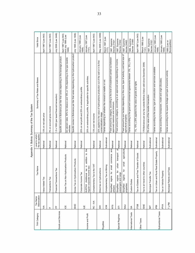
33
TAX
Cat
egor
yTa
x N
ame
Abb
revi
atio
nTa
x N
ame
Leve
l to
whi
ch
the
tax
appl
ies
Sum
mar
y of
Tax
Rat
es a
nd B
ases
Valid
Sin
ce
IVA
Valu
e A
dded
Tax
Nat
iona
l13
% o
n ne
t sal
e pr
ice
Apr
il 19
87 (L
aw 8
43)
ITTr
ansa
ctio
ns T
axN
atio
nal
3% o
n ac
crue
d gr
oss
inco
me
Apr
il 19
87 (L
aw 8
43)
ITF
Fina
ncia
l Tra
nsac
tions
Tax
Nat
iona
l1,
5 x
1000
(per
taxe
d fin
anci
al tr
ansa
ctio
n)Ju
ly 2
006
(Law
344
6)
Spec
ific
exci
se in
Bol
ivia
nos
per l
iter t
hat v
arie
s de
pend
ing
on th
e be
vera
ge p
rodu
ct.
Ad v
alor
em ra
tes:
50%
for t
obac
co a
nd 1
8% o
r 10%
dep
endi
ng o
n th
e ty
pe ta
xabl
e ve
hicl
es.
IEH
DEx
cise
Tax
on
Hyd
roca
rbon
Pro
duct
sN
atio
nal
Spec
ific
exci
se in
Bol
ivia
nos
per l
iter t
hat v
arie
s de
pend
ing
on th
e hy
droc
arbo
n pr
oduc
tJu
ly 1
995
(Law
160
6)
Cor
pora
te In
com
e Ta
xN
atio
nal
25%
on
net p
rofit
and
25%
on
extra
ordi
nary
pro
fits
Janu
ary
1995
(Law
16
06).
SUR
TAX
(Add
ition
alta
xin
addi
tion
toth
ere
gula
r cor
pora
te in
com
e ta
x)25
% o
n ex
traor
dina
ry p
rofit
s, if
app
licab
le fo
r spe
cific
act
iviti
es.
Janu
ary
1997
(Law
17
31).
RC
- IV
AC
ompl
emen
tary
Tax
to th
e VA
TN
atio
nal
13%
ove
r net
inco
me
Apr
il 19
87 (L
aw 8
43)
IDH
Dire
ct ta
x on
hyd
roca
rbon
sN
atio
nal
32%
app
lied
to th
e va
lue
of h
ydro
carb
ons
prod
uctio
n ou
t of t
he w
ell o
r in
its fi
rst
com
erci
aliz
atio
n st
age.
May
200
5 (L
aw 3
058)
ICM
Com
plem
enta
ry T
ax o
n M
inin
gSu
bnat
iona
lVa
ries
depe
ndin
g on
whe
ther
the
min
eral
is m
etal
lic o
r not
.M
arch
199
7 (L
aw
1777
)
RTS
Sim
plifi
edre
gim
efo
rsm
all
com
mer
cean
dar
tisan
sN
atio
nal
Fixe
d am
ount
by
cate
gory
, acc
ordi
ng to
the
leve
l of i
nves
tmen
t car
ried
out b
etw
een
appr
oved
max
imum
and
min
imum
.19
87. S
upre
me
Dec
ree
2152
1
STI
Sim
plifi
edre
gim
efo
rur
ban
trans
port
ofpa
ssen
gers
and
car
goN
atio
nal
Fixe
d am
ount
by
cate
gory
, acc
ordi
ng to
an
appr
oved
sca
le d
epen
ding
on
inco
me.
1987
. Sup
rem
e D
ecre
e 21
642
RAU
Sim
plifi
edre
gim
efo
rsm
all
agric
ultu
ral
prop
ertie
sN
atio
nal
Fixe
d am
ount
by
por h
ecta
re d
epen
ding
on
the
zone
, typ
e of
act
ivity
y a
nd la
nd s
ize
of
agric
ultu
ral p
rope
rty19
87. S
upre
me
decr
ee 2
4463
Inte
rnat
iona
l Tra
deG
AC
usto
m D
utie
sN
atio
nal
Varie
s ac
cord
ing
to th
e go
od a
nd c
omm
erci
al a
gree
men
ts b
etw
en 0
%,
5% y
10%
1985
. Sup
rem
e D
ecre
e 2
1060
ITG
BTa
x on
Est
ates
and
Fre
e Tr
ansf
er o
f Goo
dsN
atio
nal
1%
, 10%
y 2
0% a
pplie
d to
the
valu
e of
goo
ds a
nd ri
ghts
Apr
il 19
87 (L
aw 8
43)
ISAE
Tax
to a
ir tra
vel t
o ot
her c
ount
ries
Nat
iona
l17
6 Bo
livia
nos
per a
ny tr
ip o
utsi
de B
oliv
ia (V
alue
val
id s
ince
Dec
embe
r 200
6)M
arch
199
0 (L
aw
1141
)
IMT
Mun
icip
al T
rans
fer T
axSu
bnat
iona
l3%
of t
he v
alue
of t
he tr
ansf
er tr
ansa
ctio
n19
87. S
upre
me
Dec
ree
2152
1
IPBI
Tax
on U
rban
and
Rur
al R
eal E
stat
e Pr
oper
tySu
bnat
iona
lVa
ries
acco
rdin
g to
the
zone
, typ
e of
con
stru
ctio
n an
d se
rvic
es a
vaila
ble
Janu
ary
1995
(Law
16
06)
IPVA
Tax
on V
ehic
le P
rope
rtySu
bnat
iona
lVa
ries
acco
rdin
g to
hor
sepo
wer
, mod
el a
nd o
rigin
(Esc
alas
).Ja
nuar
y 19
95 (L
aw
1606
)
T y
PMM
unic
ipal
Pat
ents
and
Fee
sSu
bnat
iona
lVa
ries
acco
rdin
g to
the
squa
re fo
otag
e an
d ty
pe o
f eco
nom
ic a
ctiv
ity19
99 (L
aw o
n M
unic
ipal
ities
)
Oth
er T
axes
Roy
altie
s
Spec
ial R
egim
es
Subn
antio
nal T
axes
IUE
Inco
me
and
Prof
it
App
endi
x 1:
Bol
ivia
: Sum
mar
y of
the
Tax
Syst
em
Goo
ds a
nd S
ervi
ces
ICE
Exci
se T
ax o
n N
on H
ydro
carb
on P
rodu
cts
Nat
iona
lA
pril
1987
(Law
843
) an
d Ju
ly 1
995
(Law
16
06)
34
III. MONETARY POLICY TRANSMISSION IN BOLIVIA1
A. Introduction
1. Although Bolivia has succeeded in achieving low single digit inflation, looking forward, it faces a number of challenges in the conduct of its monetary policy. Following hyperinflation in the mid 1980s, inflation was brought down from about 25 percent in the early 1990s to under 5 percent in recent years, with the crawling peg exchange rate regime playing a central role. Nonetheless, the central bank now faces new challenges, in particular those related to strong pressures for real exchange rate appreciation—and the associated inflationary effects—stemming from large current account inflows.
2. Managing emerging real exchange rate pressures to protect macroeconomic stability will require the central bank to use all its policy instruments, including greater exchange rate flexibility. Given the upward exchange rate pressures and government commitment to low inflation as a national asset, it is crucial to identify the links between monetary policy instruments and key economic variables to ensure that appropriate measures are taken in a forward looking manner. The preliminary analysis of the channels for the transmission of monetary policy in Bolivia is two-pronged. First, a qualitative assessment is provided of the effectiveness of individual channels for monetary policy transmission in the Bolivian economy. Second, a vector autoregression (VAR) model is used to assess the impact of shocks to monetary policy instruments—namely interest rates, exchange rate, and narrow money—on output and prices.
3. The analysis suggests the exchange rate channel has been the strongest for monetary policy transmission in Bolivia, partly on account of high dollarization, while other channels need to be strengthened. Prices are found to be affected mainly by the nominal effective exchange rate, while output is found to be influenced only by narrow money, though to a small degree. However, as more exchange rate flexibility is needed to effectively manage large current account inflows, the central bank will no longer be able to rely on the exchange rate to serve as the nominal anchor for the economy and will therefore need to enhance monetary policy transmission through other channels.
4. The chapter is organized as follows. Section B provides the institutional context and summarizes key monetary developments; section C discusses the channels for monetary transmission in Bolivia; section D presents the empirical analysis using a VAR model; and section E concludes.
1 Prepared by Laura Jaramillo Mayor.
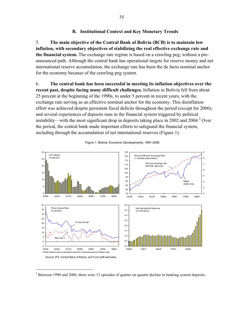
35
B. Institutional Context and Key Monetary Trends
5. The main objective of the Central Bank of Bolivia (BCB) is to maintain low inflation, with secondary objectives of stabilizing the real effective exchange rate and the financial system. The exchange rate regime is based on a crawling peg, without a pre-announced path. Although the central bank has operational targets for reserve money and net international reserve accumulation, the exchange rate has been the de facto nominal anchor for the economy because of the crawling peg system.
6. The central bank has been successful in meeting its inflation objectives over the recent past, despite facing many difficult challenges. Inflation in Bolivia fell from about 25 percent at the beginning of the 1990s, to under 5 percent in recent years, with the exchange rate serving as an effective nominal anchor for the economy. This disinflation effort was achieved despite persistent fiscal deficits throughout the period (except for 2006), and several experiences of deposits runs in the financial system triggered by political instability—with the most significant drop in deposits taking place in 2002 and 2004.2 Over the period, the central bank made important efforts to safeguard the financial system, including through the accumulation of net international reserves (Figure 1).
Figure 1. Bolivia: Economic Developments, 1991-2006
Source: IFS, Central Bank of Bolivia, and Fund staff estimates.
CPI Inflation(In percent)
0
5
10
15
20
25
30
33328 34242 35155 36068 36981 37894 38807
Nominal Effective Exchange Rate(+ indicates depreciation)
75
80
85
90
95
100
105
110
115
120
125
33328 34242 35155 36068 36981 37894 388072
3
4
5
6
7
8
9
NEER(2000=100)
Nominal exchange rate(Bs/US$, right axis)
Policy Interest Rate(In percent)
-5
0
5
10
15
20
25
30
35
40
33328 34242 35155 36068 36981 37894 38807
91-day bill rate
Real rate 1/
1/ Real interest rate is calculated using the contemporaneous inflation rate.
Net International Reserves(In US$ billion)
0.0
0.5
1.0
1.5
2.0
2.5
3.0
3.5
4.0
34699 35611 36525 37437 38352
2 Between 1990 and 2006, there were 13 episodes of quarter on quarter decline in banking system deposits.
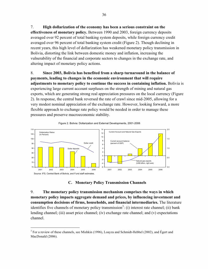
36
7. High dollarization of the economy has been a serious constraint on the effectiveness of monetary policy. Between 1990 and 2003, foreign currency deposits averaged over 92 percent of total banking system deposits, while foreign currency credit averaged over 96 percent of total banking system credit (Figure 2). Though declining in recent years, this high level of dollarization has weakened monetary policy transmission in Bolivia, distorting the link between domestic money and inflation, increasing the vulnerability of the financial and corporate sectors to changes in the exchange rate, and altering impact of monetary policy actions.
8. Since 2003, Bolivia has benefited from a sharp turnaround in the balance of payments, leading to changes in the economic environment that will require adjustments to monetary policy to continue the success in containing inflation. Bolivia is experiencing large current account surpluses on the strength of mining and natural gas exports, which are generating strong real appreciation pressures on the local currency (Figure 2). In response, the central bank reversed the rate of crawl since mid-2005, allowing for a very modest nominal appreciation of the exchange rate. However, looking forward, a more flexible approach to exchange rate policy would be needed in order to manage these pressures and preserve macroeconomic stability.
Figure 2. Bolivia: Dollarization and External Developments, 2001-2006
Source: IFS, Central Bank of Bolivia, and Fund staff estimates.
Current Account and Natural Gas Exports
-6
-4
-2
0
2
4
6
8
10
12
14
2001 2002 2003 2004 2005 20060.0
0.5
1.0
1.5
2.0
Current account balance(percent of GDP)
Natural gas exports(US$ billion, right axis)
Dollarization Ratios(In Percent)
70
75
80
85
90
95
100
105
110
2001 2002 2003 2004 2005 2006
Dollar credit
Dollar deposits
C. Monetary Policy Transmission Channels
9. The monetary policy transmission mechanism comprises the ways in which monetary policy impacts aggregate demand and prices, by influencing investment and consumption decisions of firms, households, and financial intermediaries. The literature identifies five channels of monetary policy transmission3: (i) interest rate channel; (ii) bank lending channel; (iii) asset price channel; (iv) exchange rate channel; and (v) expectations channel.
3 For a review of these channels, see Mishkin (1996), Loayza and Schmidt-Hebbel (2002), and Égert and MacDonald (2006).
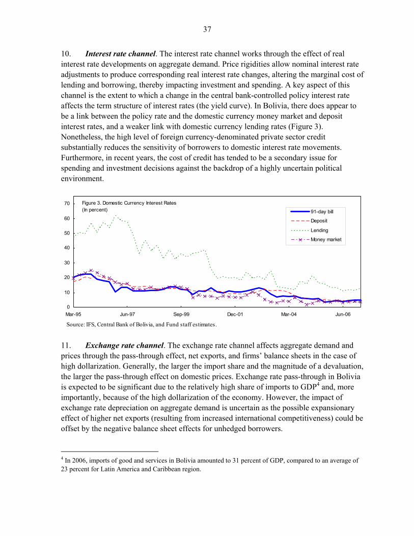
37
10. Interest rate channel. The interest rate channel works through the effect of real interest rate developments on aggregate demand. Price rigidities allow nominal interest rate adjustments to produce corresponding real interest rate changes, altering the marginal cost of lending and borrowing, thereby impacting investment and spending. A key aspect of this channel is the extent to which a change in the central bank-controlled policy interest rate affects the term structure of interest rates (the yield curve). In Bolivia, there does appear to be a link between the policy rate and the domestic currency money market and deposit interest rates, and a weaker link with domestic currency lending rates (Figure 3). Nonetheless, the high level of foreign currency-denominated private sector credit substantially reduces the sensitivity of borrowers to domestic interest rate movements. Furthermore, in recent years, the cost of credit has tended to be a secondary issue for spending and investment decisions against the backdrop of a highly uncertain political environment.
Source: IFS, Central Bank of Bolivia, and Fund staff estimates.
Figure 3. Domestic Currency Interest Rates(In percent)
0
10
20
30
40
50
60
70
Mar-95 Jun-97 Sep-99 Dec-01 Mar-04 Jun-06
91-day bill
Deposit
Lending
Money market
11. Exchange rate channel. The exchange rate channel affects aggregate demand and prices through the pass-through effect, net exports, and firms’ balance sheets in the case of high dollarization. Generally, the larger the import share and the magnitude of a devaluation, the larger the pass-through effect on domestic prices. Exchange rate pass-through in Bolivia is expected to be significant due to the relatively high share of imports to GDP4 and, more importantly, because of the high dollarization of the economy. However, the impact of exchange rate depreciation on aggregate demand is uncertain as the possible expansionary effect of higher net exports (resulting from increased international competitiveness) could be offset by the negative balance sheet effects for unhedged borrowers.
4 In 2006, imports of good and services in Bolivia amounted to 31 percent of GDP, compared to an average of 23 percent for Latin America and Caribbean region.
38
12. Bank lending channel. The bank lending channel operates via the influence of monetary policy on the supply of bank loans, i.e., the quantity rather than the price of credit. A contractionary monetary shock reduces bank reserves and therefore the total amount of bank credit available, leading to a fall in consumption and investment. In Bolivia, monetary policy has a limited capacity to effectively control banks’ ability to supply loans. In the context of high dollarization, banks have the option of drawing on external assets and foreign credit lines in response to interest rate differentials between domestic and foreign dollar assets.
13. Asset price channel. The asset price channel operates by way of the monetary policy impact on the net wealth of economic agents. An expansionary monetary policy lowers interest rates and makes equity markets more attractive, thereby changing firms’ market value and household wealth. The former alters the relative price of new investment spending, while the latter affects household consumption and the availability of collateral borrowing. The asset price channel is unlikely to be important in Bolivia due to the underdevelopment of its capital markets and the limited private sector reliance on market financing. Transactions of stocks and private sector bonds amounted to US$200 million in 2006, representing only 10 percent of stock market transactions, which are dominated by trading of government paper.
14. Expectations channel. The expectations channel works through its impact on agents’ perceptions of the economic outlook. The basis for this channel is that variables that have an intertemporal dimension—and are therefore influenced by forward-looking considerations—are affected by agents’ beliefs about future shocks to the economy and how the central bank will react to them. In this way, the expectations channel shortens the reaction lag of the other transmission channels. Accordingly, the credibility of monetary policy is crucial to this transmission channel. In Bolivia, the expectations channel associated with the exchange rate played an important role in lowering inflation, due to its strong signaling effect on the economy. However, in a context in which the exchange rate could no longer serve as the nominal anchor, expectations would be determined by the central bank’s ability to continue to meet its inflation objectives.
39
D. Empirical Analysis
15. This section examines the empirical relationship between monetary policy variables and both output and prices. Based on a conventional vector autoregression (VAR) model, Granger causality tests and generalized impulse responses are used to provide some insight into the relative strengths of the most important transmission channels. The VAR approach places minimal restrictions on how monetary shocks affect the economy, explicitly recognizing the simultaneity between monetary policy and macroeconomic developments, as well as the dependence of economic variables on monetary policy.
16. The analysis considers the effects of three policy instruments—namely interest rates, exchange rate, and domestic narrow money—on output and prices. The policy interest rate chosen for the analysis is the 91-day bill rate, as it is the key short-term interest rate used by the BCB in its open market operations throughout the sample period. The nominal effective exchange rate (NEER) is used as opposed to the bilateral exchange rate against the U.S. dollar in order to better capture the authorities’ intention of adjusting the crawling peg to maintain competitiveness with respect to Bolivia’s main trading partners. Also, the NEER is preferred over the real effective exchange rate in order to better distinguish the exchange rate channel from other transmission channels. Domestic narrow money (M1) is used instead of broad money, as it is the monetary aggregate that the authorities can influence most directly. Output is measured as real GDP excluding mining and hydrocarbons, in order to focus on the sectors that can potentially be influenced by monetary policy.5 The consumer price index is taken as the measure of the general price level. All data series are in quarterly frequency and cover the period March 1990 to December 2006.6
17. The stationarity properties of the data were tested, and the lag length of the VAR estimation was selected using Akaike (AIC) and Schwartz (SC) information criteria. The Augmented Dickey-Fuller test indicates that the variables are I(1), suggesting the presence of unit roots. Nonetheless, the analysis was conducted in levels to allow for implicit cointegrating relationships in the data.7 Both the AIC and SC tests suggest a lag of the first order, and the Lagrange Multiplier test shows that the residuals are not serially correlated.
5 Investment and overall performance in the mining and hydrocarbons sectors in Bolivia is determined to large extent by international prices, taxation policy, and long-term bilateral agreements with trading partners. 6 Data series come from the IFS database and the Central Bank of Bolivia. All data are expressed in natural logs and are seasonally adjusted using ARIMA X12, with the exception of the interest rate. 7 Sims, Stock, and Watson (1990) show that an analysis in levels is valid if enough of the variables are cointegrated, because the ordinary least squares estimator of the reduced-form VAR efficiently estimates the cointegrating relationship.
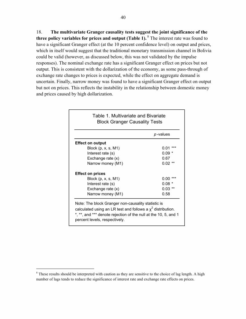
40
18. The multivariate Granger causality tests suggest the joint significance of the three policy variables for prices and output (Table 1). 8 The interest rate was found to have a significant Granger effect (at the 10 percent confidence level) on output and prices, which in itself would suggest that the traditional monetary transmission channel in Bolivia could be valid (however, as discussed below, this was not validated by the impulse responses). The nominal exchange rate has a significant Granger effect on prices but not output. This is consistent with the dollarization of the economy, as some pass-through of exchange rate changes to prices is expected, while the effect on aggregate demand is uncertain. Finally, narrow money was found to have a significant Granger effect on output but not on prices. This reflects the instability in the relationship between domestic money and prices caused by high dollarization.
Table 1. Multivariate and Bivariate Block Granger Causality Tests
p -values
Effect on outputBlock (p, x, s, M1) 0.01 ***Interest rate (s) 0.09 *Exchange rate (x) 0.67Narrow money (M1) 0.02 **
Effect on pricesBlock (p, x, s, M1) 0.00 ***Interest rate (s) 0.08 *Exchange rate (x) 0.03 **Narrow money (M1) 0.58
Note: The block Granger non-causality statistic is calculated using an LR test and follows a χ2 distribution. *, **, and *** denote rejection of the null at the 10, 5, and 1 percent levels, respectively.
8 These results should be interpreted with caution as they are sensitive to the choice of lag length. A high number of lags tends to reduce the significance of interest rate and exchange rate effects on prices.
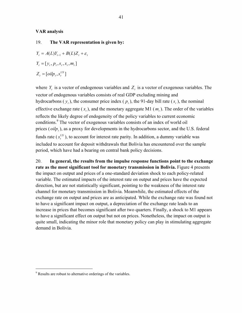
41
VAR analysis
19. The VAR representation is given by:
tttt ZLBYLAY ε++= − )()( 1
],,,,[ tttttt mxspyY =
],[ USttt soilpZ =
where tY is a vector of endogenous variables and tZ is a vector of exogenous variables. The vector of endogenous variables consists of real GDP excluding mining and hydrocarbons ( ty ), the consumer price index ( tp ), the 91-day bill rate ( ts ), the nominal effective exchange rate ( tx ), and the monetary aggregate M1 ( tm ). The order of the variables reflects the likely degree of endogeneity of the policy variables to current economic conditions.9 The vector of exogenous variables consists of an index of world oil prices ( toilp ), as a proxy for developments in the hydrocarbons sector, and the U.S. federal
funds rate ( USts ), to account for interest rate parity. In addition, a dummy variable was
included to account for deposit withdrawals that Bolivia has encountered over the sample period, which have had a bearing on central bank policy decisions.
20. In general, the results from the impulse response functions point to the exchange rate as the most significant tool for monetary transmission in Bolivia. Figure 4 presents the impact on output and prices of a one-standard deviation shock to each policy-related variable. The estimated impacts of the interest rate on output and prices have the expected direction, but are not statistically significant, pointing to the weakness of the interest rate channel for monetary transmission in Bolivia. Meanwhile, the estimated effects of the exchange rate on output and prices are as anticipated. While the exchange rate was found not to have a significant impact on output, a depreciation of the exchange rate leads to an increase in prices that becomes significant after two quarters. Finally, a shock to M1 appears to have a significant effect on output but not on prices. Nonetheless, the impact on output is quite small, indicating the minor role that monetary policy can play in stimulating aggregate demand in Bolivia.
9 Results are robust to alternative orderings of the variables.
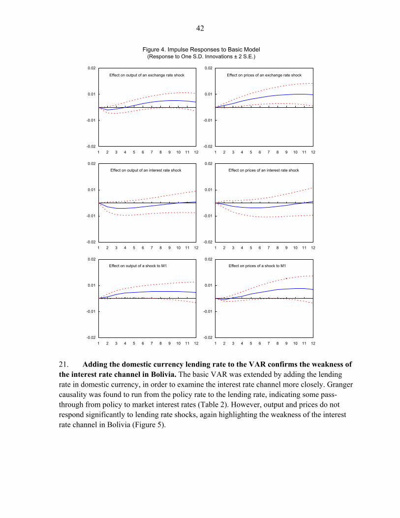
42
Figure 4. Impulse Responses to Basic Model(Response to One S.D. Innovations ± 2 S.E.)
Effect on output of an exchange rate shock
-0.02
-0.01
0.01
0.02
1 2 3 4 5 6 7 8 9 10 11 12
Effect on output of an interest rate shock
-0.02
-0.01
0.01
0.02
1 2 3 4 5 6 7 8 9 10 11 12
Effect on output of a shock to M1
-0.02
-0.01
0.01
0.02
1 2 3 4 5 6 7 8 9 10 11 12
Effect on prices of an exchange rate shock
-0.02
-0.01
0.01
0.02
1 2 3 4 5 6 7 8 9 10 11 12
Effect on prices of an interest rate shock
-0.02
-0.01
0.01
0.02
1 2 3 4 5 6 7 8 9 10 11 12
Effect on prices of a shock to M1
-0.02
-0.01
0.01
0.02
1 2 3 4 5 6 7 8 9 10 11 12
21. Adding the domestic currency lending rate to the VAR confirms the weakness of the interest rate channel in Bolivia. The basic VAR was extended by adding the lending rate in domestic currency, in order to examine the interest rate channel more closely. Granger causality was found to run from the policy rate to the lending rate, indicating some pass-through from policy to market interest rates (Table 2). However, output and prices do not respond significantly to lending rate shocks, again highlighting the weakness of the interest rate channel in Bolivia (Figure 5).
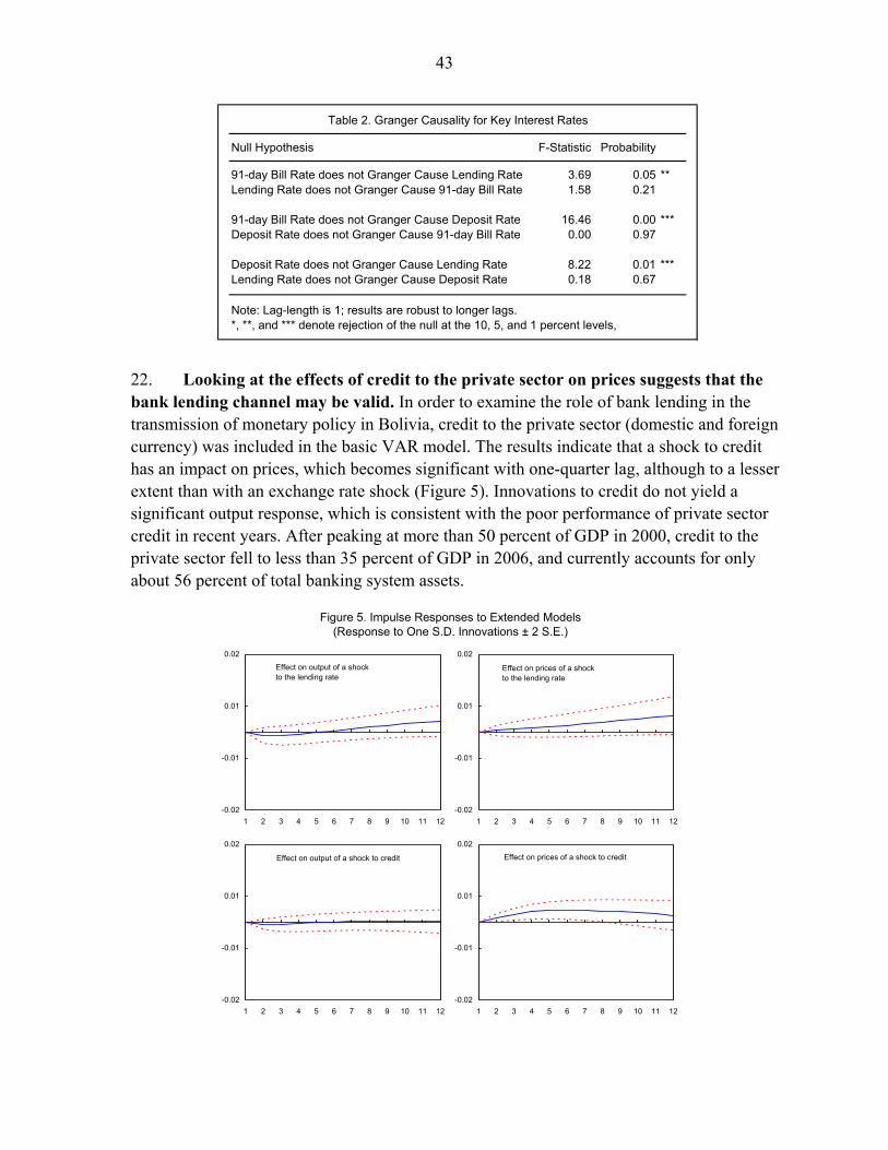
43
Null Hypothesis F-Statistic Probability
91-day Bill Rate does not Granger Cause Lending Rate 3.69 0.05 **Lending Rate does not Granger Cause 91-day Bill Rate 1.58 0.21
91-day Bill Rate does not Granger Cause Deposit Rate 16.46 0.00 ***Deposit Rate does not Granger Cause 91-day Bill Rate 0.00 0.97
Deposit Rate does not Granger Cause Lending Rate 8.22 0.01 ***Lending Rate does not Granger Cause Deposit Rate 0.18 0.67
Note: Lag-length is 1; results are robust to longer lags.*, **, and *** denote rejection of the null at the 10, 5, and 1 percent levels,
Table 2. Granger Causality for Key Interest Rates
22. Looking at the effects of credit to the private sector on prices suggests that the bank lending channel may be valid. In order to examine the role of bank lending in the transmission of monetary policy in Bolivia, credit to the private sector (domestic and foreign currency) was included in the basic VAR model. The results indicate that a shock to credit has an impact on prices, which becomes significant with one-quarter lag, although to a lesser extent than with an exchange rate shock (Figure 5). Innovations to credit do not yield a significant output response, which is consistent with the poor performance of private sector credit in recent years. After peaking at more than 50 percent of GDP in 2000, credit to the private sector fell to less than 35 percent of GDP in 2006, and currently accounts for only about 56 percent of total banking system assets.
Figure 5. Impulse Responses to Extended Models(Response to One S.D. Innovations ± 2 S.E.)
Effect on output of a shock to the lending rate
-0.02
-0.01
0.01
0.02
1 2 3 4 5 6 7 8 9 10 11 12
Effect on output of a shock to credit
-0.02
-0.01
0.01
0.02
1 2 3 4 5 6 7 8 9 10 11 12
Effect on prices of a shock to the lending rate
-0.02
-0.01
0.01
0.02
1 2 3 4 5 6 7 8 9 10 11 12
Effect on prices of a shock to credit
-0.02
-0.01
0.01
0.02
1 2 3 4 5 6 7 8 9 10 11 12
44
E. Conclusions and Policy Implications
23. While the exchange rate has been found to be the strongest channel for monetary policy transmission in Bolivia, looking forward, the central bank will face the need to strengthen other channels. The empirical results indicate that prices have been affected mainly by the nominal effective exchange rate and to a much lesser extent by bank lending. Meanwhile, output was found to be affected only to a small degree by shocks to narrow money. In the short term, the real appreciation pressures would facilitate low inflation, to the extent that they are reflected in nominal exchange rate appreciation.
24. Over the medium term, additional measures would be needed in order to enhance the effectiveness of transmission channels, particularly in the event of a reversal of the appreciation trends. Key policy challenges will include deepening financial intermediation and fostering a continued reduction of dollarization. However, this may take time, therefore it will be essential to maintain financial policies consistent with external stability (thereby forestalling depreciation pressures), in particular a prudent fiscal stance.
References
Égert, Balázs, and Ronald MacDonald, 2006, “Monetary Transmission Mechanism in Transition Economies: Surveying the Surveyable,” CESifo Working Paper No. 1739 (June).
Loayza, Norman, and Klaus Schmidt-Hebbel, eds. 2002, Monetary Policy: Rules and Transmission Mechanisms (Santiago: Central Bank of Chile.)
Mishkin, Frederic, 1996, “The Channels of Monetary Transmission: Lessons for Monetary Policy,” NBER Working Paper No. 5464 (February).
––––––, 2001, “The Transmission Mechanism and the Role of Asset Prices in Monetary Policy,” NBER Working Paper No. 8617 (December).
Sims, Christopher, James Stock, and Mark Watson, 1990, “Inference in Linear Time Series Models with Some Unit Roots,” Econometrica, Vol. 58 (January), pp. 113–144.
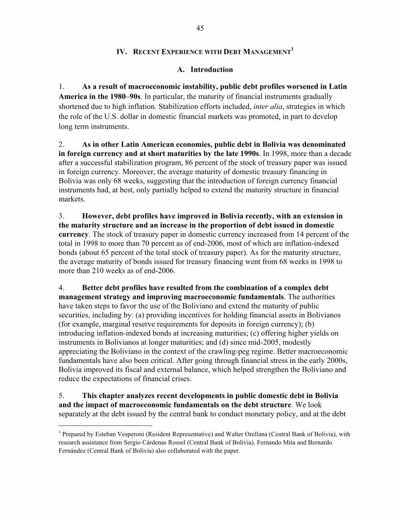
45
IV. RECENT EXPERIENCE WITH DEBT MANAGEMENT1
A. Introduction
1. As a result of macroeconomic instability, public debt profiles worsened in Latin America in the 1980–90s. In particular, the maturity of financial instruments gradually shortened due to high inflation. Stabilization efforts included, inter alia, strategies in which the role of the U.S. dollar in domestic financial markets was promoted, in part to develop long term instruments.
2. As in other Latin American economies, public debt in Bolivia was denominated in foreign currency and at short maturities by the late 1990s. In 1998, more than a decade after a successful stabilization program, 86 percent of the stock of treasury paper was issued in foreign currency. Moreover, the average maturity of domestic treasury financing in Bolivia was only 68 weeks, suggesting that the introduction of foreign currency financial instruments had, at best, only partially helped to extend the maturity structure in financial markets.
3. However, debt profiles have improved in Bolivia recently, with an extension in the maturity structure and an increase in the proportion of debt issued in domestic currency. The stock of treasury paper in domestic currency increased from 14 percent of the total in 1998 to more than 70 percent as of end-2006, most of which are inflation-indexed bonds (about 65 percent of the total stock of treasury paper). As for the maturity structure, the average maturity of bonds issued for treasury financing went from 68 weeks in 1998 to more than 210 weeks as of end-2006.
4. Better debt profiles have resulted from the combination of a complex debt management strategy and improving macroeconomic fundamentals. The authorities have taken steps to favor the use of the Boliviano and extend the maturity of public securities, including by: (a) providing incentives for holding financial assets in Bolivianos (for example, marginal reserve requirements for deposits in foreign currency); (b) introducing inflation-indexed bonds at increasing maturities; (c) offering higher yields on instruments in Bolivianos at longer maturities; and (d) since mid-2005, modestly appreciating the Boliviano in the context of the crawling-peg regime. Better macroeconomic fundamentals have also been critical. After going through financial stress in the early 2000s, Bolivia improved its fiscal and external balance, which helped strengthen the Boliviano and reduce the expectations of financial crises.
5. This chapter analyzes recent developments in public domestic debt in Bolivia and the impact of macroeconomic fundamentals on the debt structure. We look separately at the debt issued by the central bank to conduct monetary policy, and at the debt 1 Prepared by Esteban Vesperoni (Resident Representative) and Walter Orellana (Central Bank of Bolivia), with research assistance from Sergio Cárdenas Rossel (Central Bank of Bolivia). Fernando Mita and Bernardo Fernández (Central Bank of Bolivia) also collaborated with the paper.
46
issued by the treasury to finance its operations. We find that the authorities’ debt management strategy and the improvement in macroeconomic fundamentals have both played a critical role in improving debt profiles—mainly by extending maturities and shifting the currency composition towards domestic currency. We also compare debt profiles with other countries in Latin America, and found that there is still room for improvement, both in terms of maturity and currency composition.
6. The chapter is organized as follows. Section B describes institutional arrangements to manage public domestic debt in Bolivia. Section C reviews recent trends in domestic treasury paper; both issued to conduct monetary policy and treasury financing. Section D analyzes the evolution of yields on public securities. Section E compares public debt dollarization and the maturity structure in Bolivia with other Latin American countries. Section F presents econometric evidence on the effect of economic fundamentals on the debt profile. Section G concludes.
B. Domestic Debt: Institutional Arrangements
7. Domestic debt is issued for both monetary policy and treasury financing purposes. The Central Bank of Bolivia defines an annual monetary program and sets quarterly targets for debt placements. On a weekly basis, the bank conducts analysis of financial market liquidity and places debt in Open Market Operations (OMO), mainly through competitive auctions, and occasionally through its trading desk. The treasury also places debt to finance its operations, both through financing agreements with pension funds—in which the amounts and financing conditions are pre-determined—and through market placements, also conducted through a committee at the central bank.
8. The authorities place treasury bills and bonds in foreign and domestic currency. For monetary policy purposes, the central bank places treasury bills (zero-coupon bonds issued at three-, six-, and 12-month maturities) and two-year treasury bonds, mostly in domestic currency.2 The central bank also issues one- and two-year inflation-indexed treasury paper, and sporadically one-month treasury bills to curb short-term excess liquidity. The treasury concentrates on longer maturities, through six-month coupon Boliviano bonds with a pre-determined interest rate at four-, six-, and eight-year maturities.
9. Open Market Operations are conducted once a week by the Open Market Committee (OMC) and the Treasury Paper Management Committee (TPMC). These committees, which meet every Wednesday, place treasury bills and bonds in an auction process. They also review developments in domestic and international financial markets, and in particular the liquidity conditions in the financial system to set the offer of treasury paper for the following week, both for monetary and fiscal operations.
2 The central bank issues treasury bills—and not its own paper—for monetary policy purposes to avoid fragmenting a small market with different financial instruments. The proceeds from these operations are placed in a special central bank account (the Cuenta de Regulación Monetaria, whose proceeds belong to the treasury but can not be applied to its financing).
47
10. The central bank favors Open English Auctions (OEA). These were introduced in August 2005, and are conducted through an interactive auction system that operates using internet protocols. Through this auction system, participants can monitor offers from other agents in real time, giving them the opportunity to increase their bidding until closing time. OEA allows participants to obtain information during the bidding process, which reduces the “winner’s curse” effect and henceforth encourages more participation. The central bank and/or the treasury can also place public paper through the central bank’s trading desk. In general, auction mechanisms are favored, but the authorities may decide to offer paper through the latter if the monetary program so requires or if they intend to extend signals to market participants about interest rates.
11. The treasury also places long term bonds with pension funds through non-market mechanisms. The 1996 pension reform legislation grants the treasury the option to place long term bonds up to a certain share of the pension funds’ revenue.3 These are bonds with annual coupons yielding a pre-determined interest rate, the terms of which are negotiated directly between the treasury and pension funds. Up to 2002, the treasury placed U.S. dollar-indexed bonds, at a 15-year maturity, with an annual interest rate of 8 percent. Starting in 2003, and consistent with the de-dollarization strategy followed by the authorities (see below), the treasury began to place inflation-indexed bonds, with maturities between 9 and 15 years, yielding an average real interest rate of 5 percent.4
C. Recent Trends in Public Domestic Debt
12. This section reviews recent trends in public securities placed for monetary policy and treasury financing. First, it analyzes paper issued for monetary policy. Second, it focuses on treasury financing, which comprises paper auctioned through market operations and paper issued directly to pension funds. Third, it analyzes domestic debt yields.
13. Monetary policy. In the monetary policy area, the following key trends may be highlighted.
• The issuance of treasury bills has fluctuated widely, in line with the needs of monetary policy (Figures 1 and 2). Since 1997, the stock of treasury bills and bonds has been correlated with the evolution of consumer price inflation, with the exception of 2003 and 2005, years in which inflation was influenced by supply shocks.
3 A sort of call option over the pension funds’ cash flow. 4 Since early 2007, the treasury issues inflation indexed bonds only at 15-year maturity and with coupons yielding a 4 percent real interest rate.
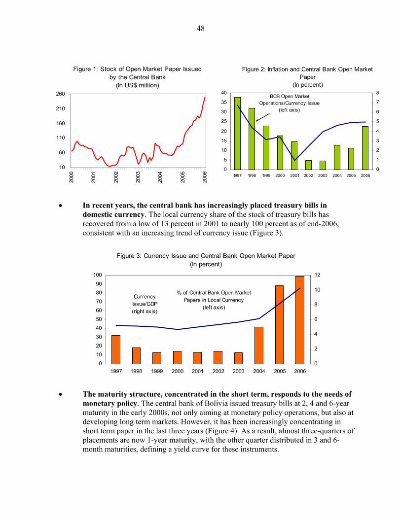
48
• In recent years, the central bank has increasingly placed treasury bills in domestic currency. The local currency share of the stock of treasury bills has recovered from a low of 13 percent in 2001 to nearly 100 percent as of end-2006, consistent with an increasing trend of currency issue (Figure 3).
• The maturity structure, concentrated in the short term, responds to the needs of monetary policy. The central bank of Bolivia issued treasury bills at 2, 4 and 6-year maturity in the early 2000s, not only aiming at monetary policy operations, but also at developing long term markets. However, it has been increasingly concentrating in short term paper in the last three years (Figure 4). As a result, almost three-quarters of placements are now 1-year maturity, with the other quarter distributed in 3 and 6-month maturities, defining a yield curve for these instruments.
0102030405060708090
100
1997 1998 1999 2000 2001 2002 2003 2004 2005 20060
2
4
6
8
10
12
Currency Issue/GDP (right axis)
% of Central Bank Open Market Papers in Local Currency
(left axis)
Figure 3: Currency Issue and Central Bank Open Market Paper(In percent)
10
60
110
160
210
260
2000
2001
2002
2003
2004
2005
2006
Figure 1: Stock of Open Market Paper Issued by the Central Bank
(In US$ million)
0
5
10
15
20
25
30
35
40
1997 1998 1999 2000 2001 2002 2003 2004 2005 20060
1
2
3
4
5
6
7
8BCB Open Market
Operations/Currency Issue(left axis)
Figure 2: Inflation and Central Bank Open Market Paper
(In percent)
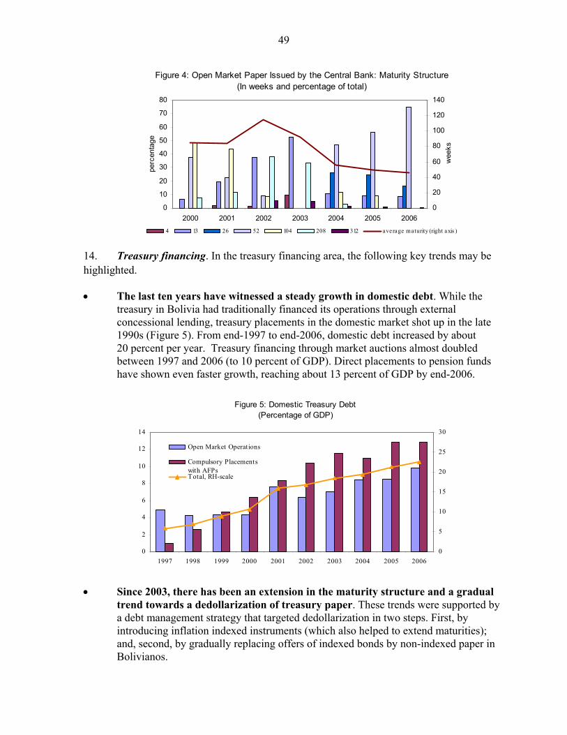
49
14. Treasury financing. In the treasury financing area, the following key trends may be highlighted.
• The last ten years have witnessed a steady growth in domestic debt. While the treasury in Bolivia had traditionally financed its operations through external concessional lending, treasury placements in the domestic market shot up in the late 1990s (Figure 5). From end-1997 to end-2006, domestic debt increased by about 20 percent per year. Treasury financing through market auctions almost doubled between 1997 and 2006 (to 10 percent of GDP). Direct placements to pension funds have shown even faster growth, reaching about 13 percent of GDP by end-2006.
0
2
4
6
8
10
12
14
1997 1998 1999 2000 2001 2002 2003 2004 2005 20060
5
10
15
20
25
30
Open Market Operations
Compulsory Placementswith AFPsTotal, RH-scale
Figure 5: Domestic Treasury Debt(Percentage of GDP)
• Since 2003, there has been an extension in the maturity structure and a gradual trend towards a dedollarization of treasury paper. These trends were supported by a debt management strategy that targeted dedollarization in two steps. First, by introducing inflation indexed instruments (which also helped to extend maturities); and, second, by gradually replacing offers of indexed bonds by non-indexed paper in Bolivianos.
0
10
20
30
40
50
60
70
80
2000 2001 2002 2003 2004 2005 2006
perc
enta
ge
0
20
40
60
80
100
120
140
wee
ks
4 13 26 52 104 208 312 average maturity (right axis )
Figure 4: Open Market Paper Issued by the Central Bank: Maturity Structure(In weeks and percentage of total)
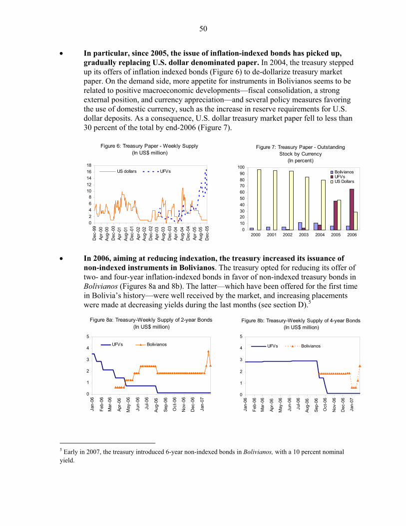
50
• In particular, since 2005, the issue of inflation-indexed bonds has picked up, gradually replacing U.S. dollar denominated paper. In 2004, the treasury stepped up its offers of inflation indexed bonds (Figure 6) to de-dollarize treasury market paper. On the demand side, more appetite for instruments in Bolivianos seems to be related to positive macroeconomic developments—fiscal consolidation, a strong external position, and currency appreciation—and several policy measures favoring the use of domestic currency, such as the increase in reserve requirements for U.S. dollar deposits. As a consequence, U.S. dollar treasury market paper fell to less than 30 percent of the total by end-2006 (Figure 7).
Figure 6: Treasury Paper - Weekly Supply(In US$ million)
02468
1012141618
Dec
-99
Apr-
00Au
g-00
Dec
-00
Apr-
01Au
g-01
Dec
-01
Apr-
02Au
g-02
Dec
-02
Apr-
03Au
g-03
Dec
-03
Apr-
04Au
g-04
Dec
-04
Apr-
05Au
g-05
Dec
-05
US dollars UFVs
• In 2006, aiming at reducing indexation, the treasury increased its issuance of non-indexed instruments in Bolivianos. The treasury opted for reducing its offer of two- and four-year inflation-indexed bonds in favor of non-indexed treasury bonds in Bolivianos (Figures 8a and 8b). The latter—which have been offered for the first time in Bolivia’s history—were well received by the market, and increasing placements were made at decreasing yields during the last months (see section D).5
0
1
2
3
4
5
Jan-
06
Feb-
06
Mar
-06
Apr-
06
May
-06
Jun-
06
Jul-0
6
Aug-
06
Sep-
06
Oct
-06
Nov
-06
Dec
-06
Jan-
07
UFVs Bolivianos
Figure 8a: Treasury-Weekly Supply of 2-year Bonds(In US$ million)
5 Early in 2007, the treasury introduced 6-year non-indexed bonds in Bolivianos, with a 10 percent nominal yield.
0
1
2
3
4
5
Jan-
06
Feb-
06
Mar
-06
Apr-
06
May
-06
Jun-
06
Jul-0
6
Aug-
06
Sep-
06
Oct
-06
Nov
-06
Dec
-06
Jan-
07UFVs Bolivianos
Figure 8b: Treasury-Weekly Supply of 4-year Bonds(In US$ million)
0102030405060708090
100
2000 2001 2002 2003 2004 2005 2006
BolivianosUFVsUS Dollars
Figure 7: Treasury Paper - Outstanding Stock by Currency
(In percent)
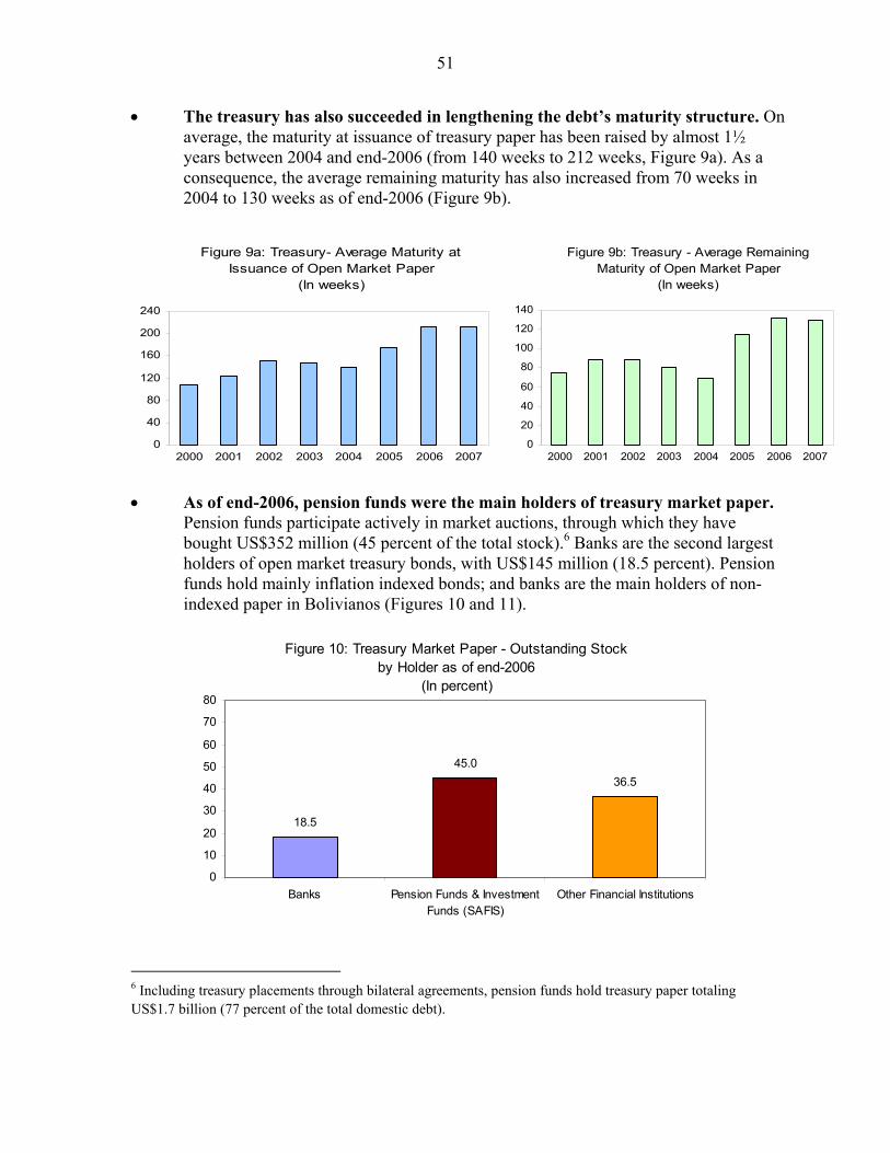
51
• The treasury has also succeeded in lengthening the debt’s maturity structure. On average, the maturity at issuance of treasury paper has been raised by almost 1½ years between 2004 and end-2006 (from 140 weeks to 212 weeks, Figure 9a). As a consequence, the average remaining maturity has also increased from 70 weeks in 2004 to 130 weeks as of end-2006 (Figure 9b).
0
40
80
120
160
200
240
2000 2001 2002 2003 2004 2005 2006 2007
Figure 9a: Treasury- Average Maturity at Issuance of Open Market Paper
(In weeks)
• As of end-2006, pension funds were the main holders of treasury market paper. Pension funds participate actively in market auctions, through which they have bought US$352 million (45 percent of the total stock).6 Banks are the second largest holders of open market treasury bonds, with US$145 million (18.5 percent). Pension funds hold mainly inflation indexed bonds; and banks are the main holders of non-indexed paper in Bolivianos (Figures 10 and 11).
18.5
45.036.5
0
10
20
30
40
50
60
70
80
Banks Pension Funds & InvestmentFunds (SAFIS)
Other Financial Institutions
Figure 10: Treasury Market Paper - Outstanding Stock by Holder as of end-2006
(In percent)
6 Including treasury placements through bilateral agreements, pension funds hold treasury paper totaling US$1.7 billion (77 percent of the total domestic debt).
0
20
40
60
80
100
120
140
2000 2001 2002 2003 2004 2005 2006 2007
Figure 9b: Treasury - Average Remaining Maturity of Open Market Paper
(In weeks)
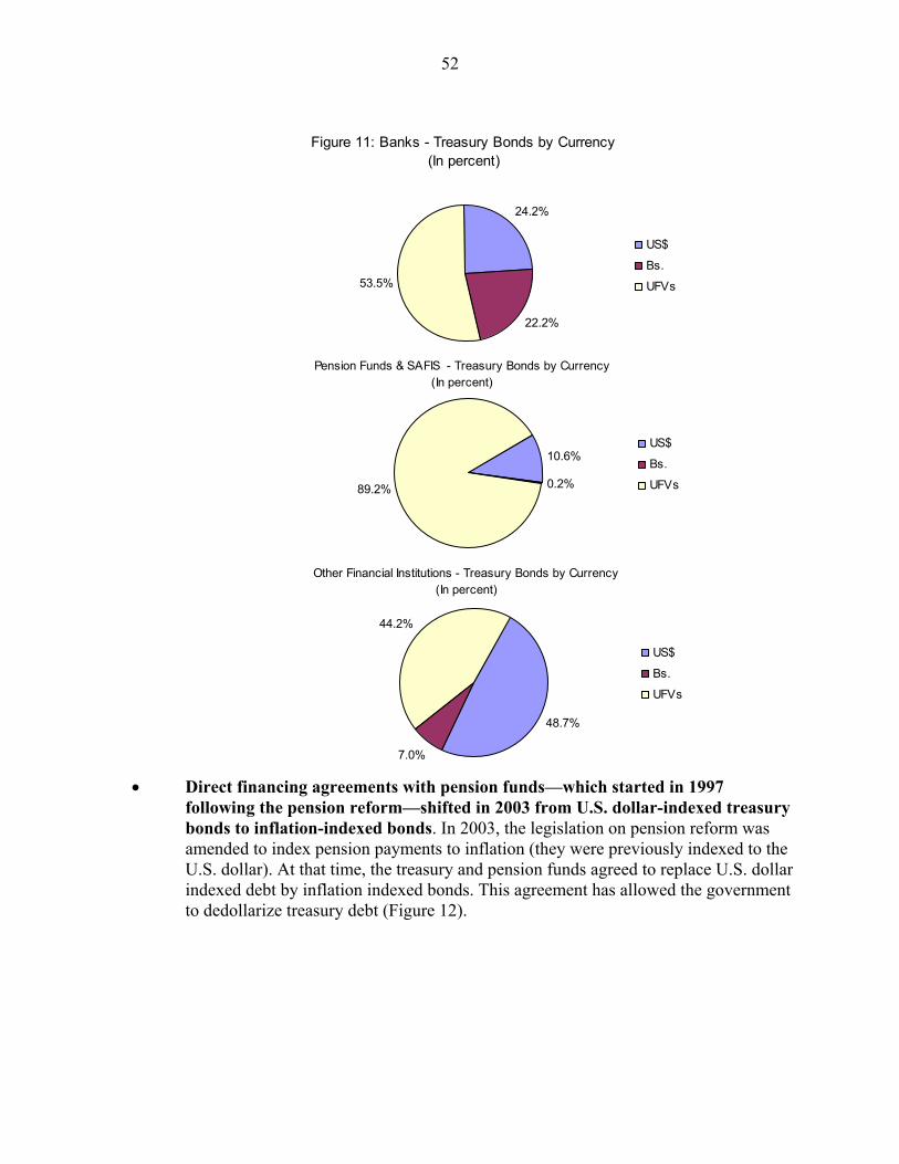
52
• Direct financing agreements with pension funds—which started in 1997 following the pension reform—shifted in 2003 from U.S. dollar-indexed treasury bonds to inflation-indexed bonds. In 2003, the legislation on pension reform was amended to index pension payments to inflation (they were previously indexed to the U.S. dollar). At that time, the treasury and pension funds agreed to replace U.S. dollar indexed debt by inflation indexed bonds. This agreement has allowed the government to dedollarize treasury debt (Figure 12).
Other Financial Institutions - Treasury Bonds by Currency (In percent)
48.7%
7.0%
44.2%
US$
Bs.
UFVs
24.2%
22.2%
53.5%
US$
Bs.
UFVs
Pension Funds & SAFIS - Treasury Bonds by Currency(In percent)
10.6%
0.2%89.2%
US$
Bs.
UFVs
Figure 11: Banks - Treasury Bonds by Currency(In percent)
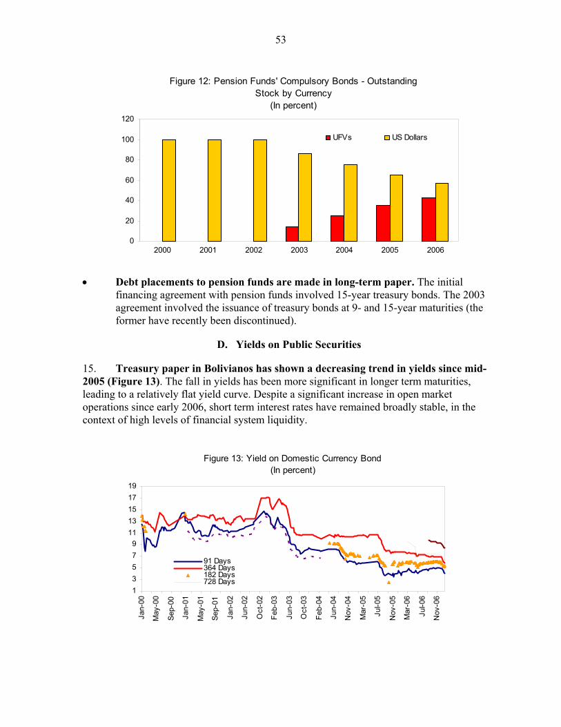
53
0
20
40
60
80
100
120
2000 2001 2002 2003 2004 2005 2006
UFVs US Dollars
Figure 12: Pension Funds' Compulsory Bonds - Outstanding Stock by Currency
(In percent)
• Debt placements to pension funds are made in long-term paper. The initial financing agreement with pension funds involved 15-year treasury bonds. The 2003 agreement involved the issuance of treasury bonds at 9- and 15-year maturities (the former have recently been discontinued).
D. Yields on Public Securities
15. Treasury paper in Bolivianos has shown a decreasing trend in yields since mid-2005 (Figure 13). The fall in yields has been more significant in longer term maturities, leading to a relatively flat yield curve. Despite a significant increase in open market operations since early 2006, short term interest rates have remained broadly stable, in the context of high levels of financial system liquidity.
13579
1113151719
Jan-
00
May
-00
Sep-
00
Jan-
01
May
-01
Sep-
01
Jan-
02
Jun-
02
Oct
-02
Feb-
03
Jun-
03
Oct
-03
Feb-
04
Jun-
04
Nov
-04
Mar
-05
Jul-0
5
Nov
-05
Mar
-06
Jul-0
6
Nov
-06
91 Days364 Days182 Days728 Days28 D
Figure 13: Yield on Domestic Currency Bond(In percent)
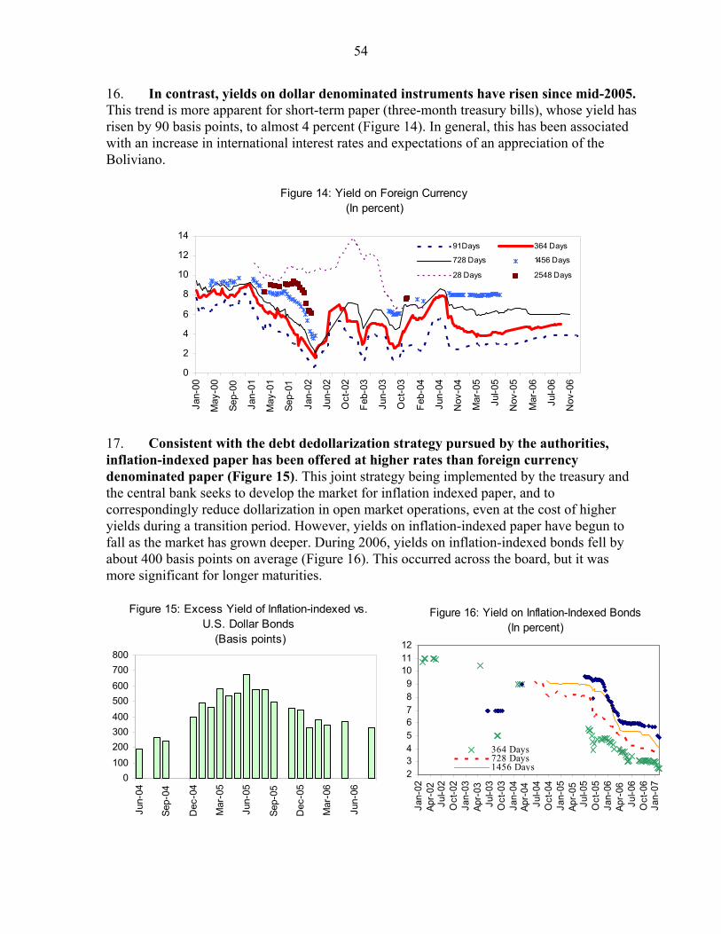
54
16. In contrast, yields on dollar denominated instruments have risen since mid-2005. This trend is more apparent for short-term paper (three-month treasury bills), whose yield has risen by 90 basis points, to almost 4 percent (Figure 14). In general, this has been associated with an increase in international interest rates and expectations of an appreciation of the Boliviano.
0
2
4
6
8
10
12
14
Jan-
00
May
-00
Sep-
00
Jan-
01
May
-01
Sep-
01
Jan-
02
Jun-
02
Oct
-02
Feb-
03
Jun-
03
Oct
-03
Feb-
04
Jun-
04
Nov
-04
Mar
-05
Jul-0
5
Nov
-05
Mar
-06
Jul-0
6
Nov
-06
91 Days 364 Days
728 Days 1456 Days
28 Days 2548 Days
Figure 14: Yield on Foreign Currency(In percent)
17. Consistent with the debt dedollarization strategy pursued by the authorities, inflation-indexed paper has been offered at higher rates than foreign currency denominated paper (Figure 15). This joint strategy being implemented by the treasury and the central bank seeks to develop the market for inflation indexed paper, and to correspondingly reduce dollarization in open market operations, even at the cost of higher yields during a transition period. However, yields on inflation-indexed paper have begun to fall as the market has grown deeper. During 2006, yields on inflation-indexed bonds fell by about 400 basis points on average (Figure 16). This occurred across the board, but it was more significant for longer maturities.
0100200300400500600700800
Jun-
04
Sep-
04
Dec
-04
Mar
-05
Jun-
05
Sep-
05
Dec
-05
Mar
-06
Jun-
06
Figure 15: Excess Yield of Inflation-indexed vs. U.S. Dollar Bonds
(Basis points)
23456789
101112
Jan-
02Ap
r-02
Jul-0
2O
ct-0
2Ja
n-03
Apr-
03Ju
l-03
Oct
-03
Jan-
04Ap
r-04
Jul-0
4O
ct-0
4Ja
n-05
Apr-
05Ju
l-05
Oct
-05
Jan-
06Ap
r-06
Jul-0
6O
ct-0
6Ja
n-07
364 Days728 Days1456 Days
Figure 16: Yield on Inflation-Indexed Bonds(In percent)
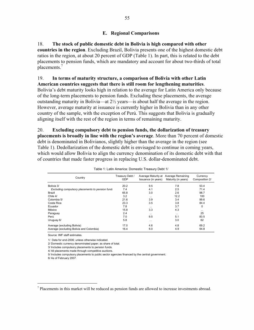
55
E. Regional Comparisons
18. The stock of public domestic debt in Bolivia is high compared with other countries in the region. Excluding Brazil, Bolivia presents one of the highest domestic debt ratios in the region, at about 20 percent of GDP (Table 1). In part, this is related to the debt placements to pension funds, which are mandatory and account for about two-thirds of total placements.7
19. In terms of maturity structure, a comparison of Bolivia with other Latin American countries suggests that there is still room for lengthening maturities. Bolivia’s debt maturity looks high in relation to the average for Latin America only because of the long-term placements to pension funds. Excluding these placements, the average outstanding maturity in Bolivia—at 2½ years—is about half the average in the region. However, average maturity at issuance is currently higher in Bolivia than in any other country of the sample, with the exception of Perú. This suggests that Bolivia is gradually aligning itself with the rest of the region in terms of remaining maturity.
20. Excluding compulsory debt to pension funds, the dollarization of treasury placements is broadly in line with the region’s average. More than 70 percent of domestic debt is denominated in Bolivianos, slightly higher than the average in the region (see Table 1). Dedollarization of the domestic debt is envisaged to continue in coming years, which would allow Bolivia to align the currency denomination of its domestic debt with that of countries that made faster progress in replacing U.S. dollar-denominated debt.
Table 1: Latin America: Domestic Treasury Debt 1/
Bolivia 3/ 20.2 9.5 7.8 53.4 Excluding compulsory placements to pension funds 7.4 4.1 2.5 71.4Brazil 65.8 3.0 2.6 98.7Chile 4/ 3.2 ... 12.2 100Colombia 5/ 21.6 3.9 3.4 99.6Costa Rica 23.3 3.5 3.8 84.4Ecuador 7.8 ... 3.7 0México 15.8 3.3 4.3 ...Paraguay 2.4 ... ... 25Perú 7.0 9.5 5.1 83.5Uruguay 6/ 5.8 … 3.0 62
Average (excluding Bolivia) 17.0 4.6 4.8 69.2Average (excluding Bolivia and Colombia) 16.4 6.0 4.9 64.8
Source: IMF staff estimates.
1/ Data for end-2006; unless otherwise indicated.2/ Domestic currency denominated paper; as share of total.3/ Includes compulsory placements to pension funds.4/ All placements made through competitive auctions.5/ Includes compulsory placements to public sector agencies financed by the central government. 6/ As of February 2007.
Currency Composition 2/Country Treasury Debt /
GDP Average Maturity at Issuance (in years)
Average Remaining Maturity (in years)
7 Placements in this market will be reduced as pension funds are allowed to increase investments abroad.
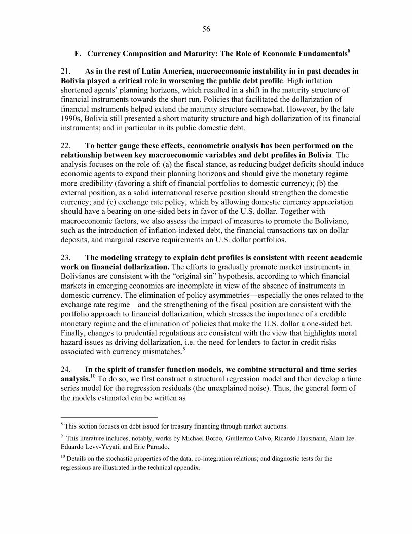
56
F. Currency Composition and Maturity: The Role of Economic Fundamentals8
21. As in the rest of Latin America, macroeconomic instability in in past decades in Bolivia played a critical role in worsening the public debt profile. High inflation shortened agents’ planning horizons, which resulted in a shift in the maturity structure of financial instruments towards the short run. Policies that facilitated the dollarization of financial instruments helped extend the maturity structure somewhat. However, by the late 1990s, Bolivia still presented a short maturity structure and high dollarization of its financial instruments; and in particular in its public domestic debt.
22. To better gauge these effects, econometric analysis has been performed on the relationship between key macroeconomic variables and debt profiles in Bolivia. The analysis focuses on the role of: (a) the fiscal stance, as reducing budget deficits should induce economic agents to expand their planning horizons and should give the monetary regime more credibility (favoring a shift of financial portfolios to domestic currency); (b) the external position, as a solid international reserve position should strengthen the domestic currency; and (c) exchange rate policy, which by allowing domestic currency appreciation should have a bearing on one-sided bets in favor of the U.S. dollar. Together with macroeconomic factors, we also assess the impact of measures to promote the Boliviano, such as the introduction of inflation-indexed debt, the financial transactions tax on dollar deposits, and marginal reserve requirements on U.S. dollar portfolios.
23. The modeling strategy to explain debt profiles is consistent with recent academic work on financial dollarization. The efforts to gradually promote market instruments in Bolivianos are consistent with the “original sin” hypothesis, according to which financial markets in emerging economies are incomplete in view of the absence of instruments in domestic currency. The elimination of policy asymmetries—especially the ones related to the exchange rate regime—and the strengthening of the fiscal position are consistent with the portfolio approach to financial dollarization, which stresses the importance of a credible monetary regime and the elimination of policies that make the U.S. dollar a one-sided bet. Finally, changes to prudential regulations are consistent with the view that highlights moral hazard issues as driving dollarization, i.e. the need for lenders to factor in credit risks associated with currency mismatches.9
24. In the spirit of transfer function models, we combine structural and time series analysis.10 To do so, we first construct a structural regression model and then develop a time series model for the regression residuals (the unexplained noise). Thus, the general form of the models estimated can be written as
8 This section focuses on debt issued for treasury financing through market auctions. 9 This literature includes, notably, works by Michael Bordo, Guillermo Calvo, Ricardo Hausmann, Alain Ize Eduardo Levy-Yeyati, and Eric Parrado. 10 Details on the stochastic properties of the data, co-integration relations; and diagnostic tests for the regressions are illustrated in the technical appendix.
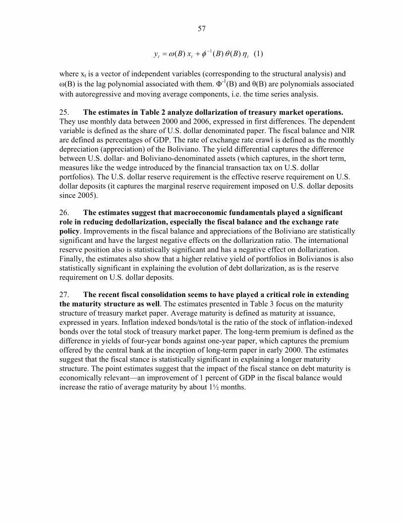
57
ttt BBxBy ηθφω )()()( 1−+= (1)
where xt is a vector of independent variables (corresponding to the structural analysis) and ω(B) is the lag polynomial associated with them. Φ-1(B) and θ(B) are polynomials associated with autoregressive and moving average components, i.e. the time series analysis.
25. The estimates in Table 2 analyze dollarization of treasury market operations. They use monthly data between 2000 and 2006, expressed in first differences. The dependent variable is defined as the share of U.S. dollar denominated paper. The fiscal balance and NIR are defined as percentages of GDP. The rate of exchange rate crawl is defined as the monthly depreciation (appreciation) of the Boliviano. The yield differential captures the difference between U.S. dollar- and Boliviano-denominated assets (which captures, in the short term, measures like the wedge introduced by the financial transaction tax on U.S. dollar portfolios). The U.S. dollar reserve requirement is the effective reserve requirement on U.S. dollar deposits (it captures the marginal reserve requirement imposed on U.S. dollar deposits since 2005).
26. The estimates suggest that macroeconomic fundamentals played a significant role in reducing dedollarization, especially the fiscal balance and the exchange rate policy. Improvements in the fiscal balance and appreciations of the Boliviano are statistically significant and have the largest negative effects on the dollarization ratio. The international reserve position also is statistically significant and has a negative effect on dollarization. Finally, the estimates also show that a higher relative yield of portfolios in Bolivianos is also statistically significant in explaining the evolution of debt dollarization, as is the reserve requirement on U.S. dollar deposits.
27. The recent fiscal consolidation seems to have played a critical role in extending the maturity structure as well. The estimates presented in Table 3 focus on the maturity structure of treasury market paper. Average maturity is defined as maturity at issuance, expressed in years. Inflation indexed bonds/total is the ratio of the stock of inflation-indexed bonds over the total stock of treasury market paper. The long-term premium is defined as the difference in yields of four-year bonds against one-year paper, which captures the premium offered by the central bank at the inception of long-term paper in early 2000. The estimates suggest that the fiscal stance is statistically significant in explaining a longer maturity structure. The point estimates suggest that the impact of the fiscal stance on debt maturity is economically relevant—an improvement of 1 percent of GDP in the fiscal balance would increase the ratio of average maturity by about 1½ months.
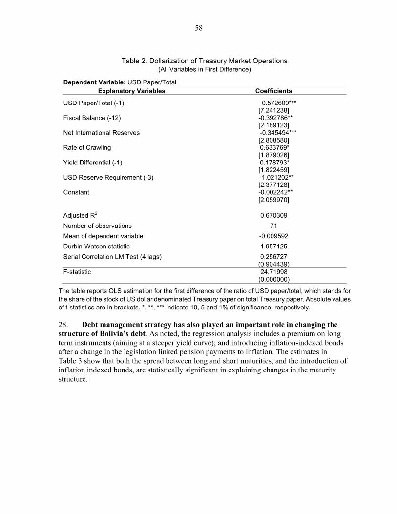
58
Table 2. Dollarization of Treasury Market Operations
(All Variables in First Difference)
Dependent Variable: USD Paper/Total Explanatory Variables Coefficients
USD Paper/Total (-1) 0.572609*** [7.241238]
Fiscal Balance (-12) -0.392786** [2.189123]
Net International Reserves -0.345494*** [2.808580]
Rate of Crawling 0.633769* [1.879026]
Yield Differential (-1) 0.178793* [1.822459]
USD Reserve Requirement (-3) -1.021202** [2.377128]
Constant -0.002242** [2.059970]
Adjusted R2 0.670309 Number of observations 71 Mean of dependent variable -0.009592 Durbin-Watson statistic 1.957125 Serial Correlation LM Test (4 lags) 0.256727
(0.904439) F-statistic 24.71998
(0.000000)
The table reports OLS estimation for the first difference of the ratio of USD paper/total, which stands for the share of the stock of US dollar denominated Treasury paper on total Treasury paper. Absolute values of t-statistics are in brackets. *, **, *** indicate 10, 5 and 1% of significance, respectively.
28. Debt management strategy has also played an important role in changing the structure of Bolivia’s debt. As noted, the regression analysis includes a premium on long term instruments (aiming at a steeper yield curve); and introducing inflation-indexed bonds after a change in the legislation linked pension payments to inflation. The estimates in Table 3 show that both the spread between long and short maturities, and the introduction of inflation indexed bonds, are statistically significant in explaining changes in the maturity structure.
59
Table 3. Maturity Structure of Treasury Market Operations
(All variables in levels)
Dependent Variable: Average Maturity Explanatory Variables Coefficients
Average Maturity (-1) 0.926960*** [50.05302]
Fiscal Balance (-12) 0.126300*** [4.940901]
Inflation-indexed Bonds/Total (-3) 0.027369*** [4.302932]
Long Term Premium (-3) 0.467604*** [5.610344]
Constant 0.025497*** [4.065238]
Moving Average Component (4) -0.552025*** [5.464450]
Adjusted R2 0.992761
Number of observations 72
Mean of dependent variable 0.406164
Durbin-Watson statistic 1.631396
Serial Correlation LM Test (4 lags) 1.506807 (0.211161)
F-statistic 1948.444 (0.000000)
The table reports OLS estimation for the average maturity at issuance of Treasury papers in Central Bank’s weekly auctions. Absolute values of t-statistics are in brackets. *, **, *** indicate 10, 5 and 1% of significance, respectively.
G. Conclusions
29. The profile of Bolivia’s domestic public debt has improved significantly in recent years. Since the late 1990s, the stock of treasury market paper in domestic currency has increased from 14 percent of the total to more than 70 percent. This has been achieved at the cost of significant increases in inflation-indexed debt. However, since early 2006, the authorities are successfully pursuing a de-indexation strategy. Meanwhile, the average maturity of treasury bonds has lengthened from 68 weeks in 1998 to more than 210 weeks.
30. Together with the authorities’ debt management strategy, better macroeconomic fundamentals have been critical in improving the profile of public debt. After going through financial stress during 2000–04—years in which the fiscal situation was highly fragile and Bolivia experienced several bank runs—the macroeconomic fundamentals have improved sharply, helped by a favorable international situation.
60
31. Nonetheless, a comparison of Bolivia with other Latin American countries suggests that there is still room for improvement. Excluding pension fund placements, the average remaining maturity in Bolivia—at 2½ years—is about half the average in the region. Average maturity at issuance, though, is currently higher in Bolivia than in any other country of the sample, with the exception of Perú, suggesting that Bolivia is gradually aligning its debt structure with those in the region. As for dollarization, Bolivia’s domestic currency composition of treasury paper is at the average in Latin America.
32. The econometric evidence suggests that, looking ahead, keeping a sound macroeconomic environment is essential for further improvements in the debt profile. Estimates based on transfer function models that combine structural and time series analysis suggest that macroeconomic fundamentals—i.e., the fiscal and external positions—have played a critical role both in extending maturities and in dedollarizing financial instruments. A sound macroeconomic stance also seems essential for the authorities’ efforts towards reducing indexation of the public debt.
61
References Antelo, E., 2000, “Políticas de estabilización y de reformas estructurales en Bolivia a partir
de 1985,” Serie Reformas Económicas. Universidad Católica Boliviana. La Paz, Bolivia.
Banco Central de Bolivia, 2005, “Operaciones de mercado abierto del Banco Central de
Bolivia,” (La Paz, Bolivia: Subgerencia de Operaciones de Mercado Abierto, Gerencia de Operaciones Monetarias, Banco Central de Bolivia).
Barajas, A., and R. Morales, 2003, “Dollarization of Liabilities: Beyond the Usual Suspects,”
IMF Working Paper 03/11 (Washington: International Monetary Fund). Bordo, M., 2006, “Sudden Stops, Financial Crises and Original Sin in Emerging Countries:
Déjà vu?” Mimeo. Calvo, G., 1996, “From Currency Substitution to Dollarization and Beyond: Analytical and
Policy Issues,” in Money, Exchange Rates, and Output. The MIT Press. ––––––, A. Izquierdo, and E. Talvi, 2003, “Sudden Stops, the Real Exchange Rate, and
Fiscal Sustainability: Argentina’s Lessons,” NBER Working Paper No. 9828 (Cambridge, Massachusetts: National Bureau of Economic Research).
––––––, Reinhart, C., 2000, “Fear of Floating,” NBER Working Paper No. 7993 (Cambridge,
Massachusetts: National Bureau of Economic Research). Cavallo, Domingo, and Joaquin Cottani, 1997, “Argentina's Convertibility Plan and the
IMF,” American Economic Review, Vol. 87, No. 2, Papers and Proceedings of the Hundred and Fourth Annual Meeting of the American Economic Association, pp. 17–22.
Dolado, J., Gonzalo, and J. Marmol, F., 1999, “Cointegration,” Mimeo, Universidad
Carlos III de Madrid. Granger, C., and T. Lee, 1990, “Multicointegration,” Advanced in Econometrics, Vol.8. Hausmann, R., 2005, “Cuántas Monedas Debería Haber? Cinco o Ciento Cinco?” Los
Grandes Debates Económicos. Heymann, D., and A. Leijonhufvud, 1998, High inflation. Clarendon Press, Oxford. Ize, A., 2005, “Financial Dollarization Equilibria: A Framework for Policy Analysis,” IMF
Working Paper 05/186 (Washington: International Monetary Fund).

62
––––––, and E. Levy Yeyati, 2003b, “Financial Dollarization,” Journal of International
Economics, Vol. 59, pp. 323–47. ––––––, and E. Levy Yeyati, 2005, “Financial De-Dollarization: Is It for Real?” IMF
Working Paper 05/187 (Washington: International Monetary Fund). ––––––, and E. Parrado, 2002, “Dollarization, Monetary Policy, and the Pass-Through,” IMF
Working Paper 02/188 (Washington: International Monetary Fund). ––––––, and A. Powell, 2003a, “Prudential Responses to De Facto Dollarization,” Mimeo,
Universidad Torcuato Di Tella and World Bank. Orellana, W., and C. Mollinedo, 1997, “Percepción de Riesgo, Dolarización y Política
Monetaria en Bolivia,” (La Paz: Banco Central de Bolivia). Rennhack, R., and M. Nozaki, 2005, “Financial Dollarization in Latin America,” Mimeo,
International Monetary Fund. Schmukler, S., Estaban Vesperoni, 2004, “Financial Globalization and Debt Maturity in
Emerging Economies,” Journal of Development Economics, Vol. 79.
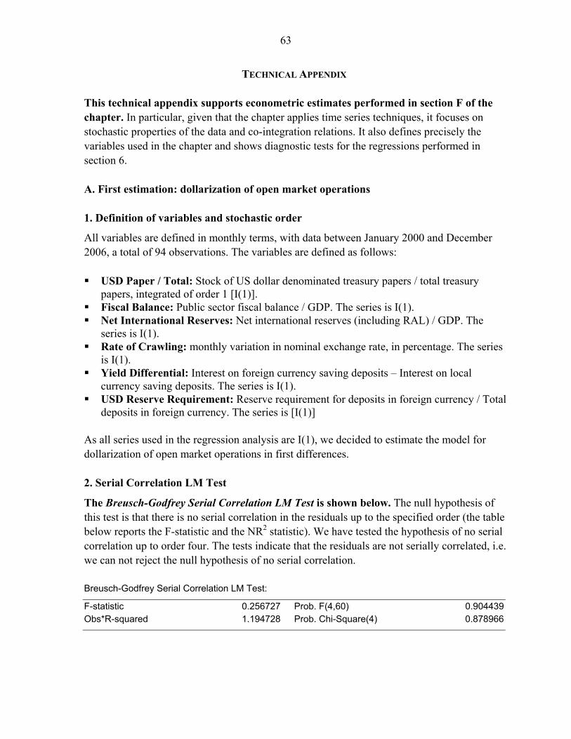
63
TECHNICAL APPENDIX This technical appendix supports econometric estimates performed in section F of the chapter. In particular, given that the chapter applies time series techniques, it focuses on stochastic properties of the data and co-integration relations. It also defines precisely the variables used in the chapter and shows diagnostic tests for the regressions performed in section 6. A. First estimation: dollarization of open market operations 1. Definition of variables and stochastic order
All variables are defined in monthly terms, with data between January 2000 and December 2006, a total of 94 observations. The variables are defined as follows: USD Paper / Total: Stock of US dollar denominated treasury papers / total treasury
papers, integrated of order 1 [I(1)]. Fiscal Balance: Public sector fiscal balance / GDP. The series is I(1). Net International Reserves: Net international reserves (including RAL) / GDP. The
series is I(1). Rate of Crawling: monthly variation in nominal exchange rate, in percentage. The series
is I(1). Yield Differential: Interest on foreign currency saving deposits – Interest on local
currency saving deposits. The series is I(1). USD Reserve Requirement: Reserve requirement for deposits in foreign currency / Total
deposits in foreign currency. The series is [I(1)] As all series used in the regression analysis are I(1), we decided to estimate the model for dollarization of open market operations in first differences. 2. Serial Correlation LM Test
The Breusch-Godfrey Serial Correlation LM Test is shown below. The null hypothesis of this test is that there is no serial correlation in the residuals up to the specified order (the table below reports the F-statistic and the NR2 statistic). We have tested the hypothesis of no serial correlation up to order four. The tests indicate that the residuals are not serially correlated, i.e. we can not reject the null hypothesis of no serial correlation. Breusch-Godfrey Serial Correlation LM Test:
F-statistic 0.256727 Prob. F(4,60) 0.904439Obs*R-squared 1.194728 Prob. Chi-Square(4) 0.878966
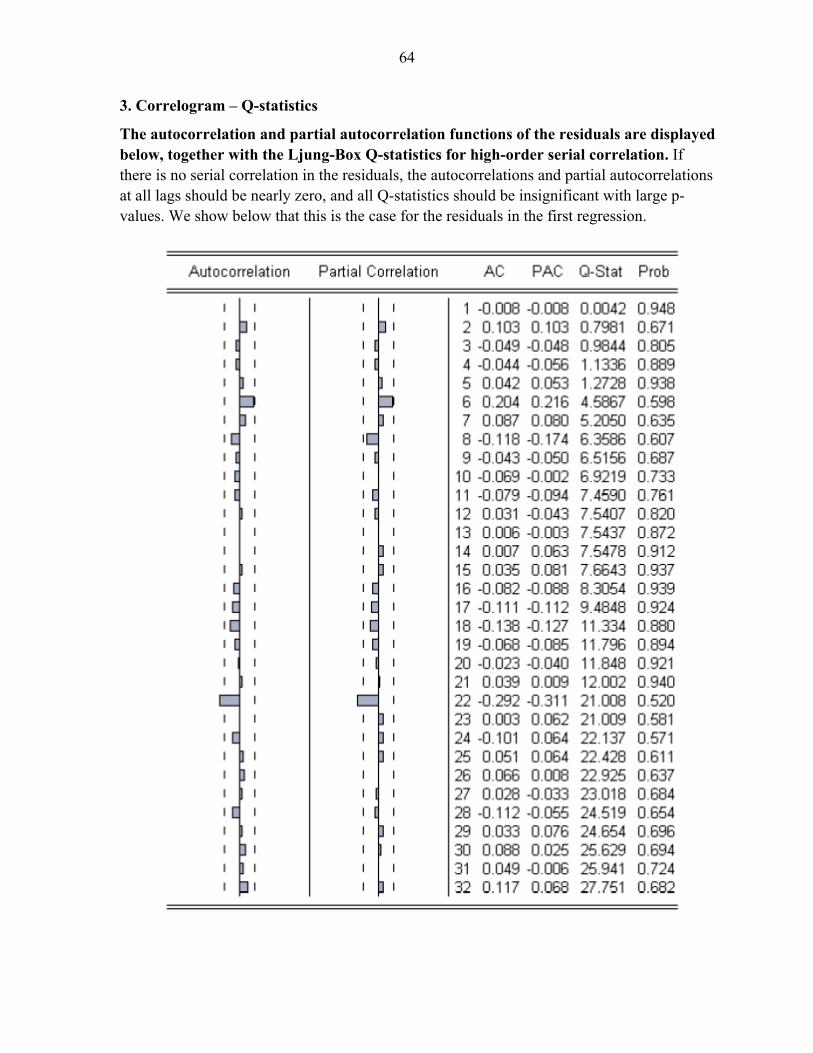
64
3. Correlogram – Q-statistics
The autocorrelation and partial autocorrelation functions of the residuals are displayed below, together with the Ljung-Box Q-statistics for high-order serial correlation. If there is no serial correlation in the residuals, the autocorrelations and partial autocorrelations at all lags should be nearly zero, and all Q-statistics should be insignificant with large p-values. We show below that this is the case for the residuals in the first regression.
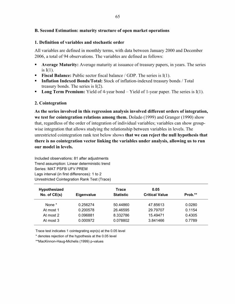
65
B. Second Estimation: maturity structure of open market operations 1. Definition of variables and stochastic order
All variables are defined in monthly terms, with data between January 2000 and December 2006, a total of 94 observations. The variables are defined as follows:
Average Maturity: Average maturity at issuance of treasury papers, in years. The series is I(1).
Fiscal Balance: Public sector fiscal balance / GDP. The series is I(1). Inflation Indexed Bonds/Total: Stock of inflation-indexed treasury bonds / Total
treasury bonds. The series is I(2). Long Term Premium: Yield of 4-year bond – Yield of 1-year paper. The series is I(1).
2. Cointegration
As the series involved in this regression analysis involved different orders of integration, we test for cointegration relations among them. Dolado (1999) and Granger (1990) show that, regardless of the order of integration of individual variables; variables can show group-wise integration that allows studying the relationship between variables in levels. The unrestricted cointegration rank test below shows that we can reject the null hypothesis that there is no cointegration vector linking the variables under analysis, allowing us to run our model in levels. Included observations: 81 after adjustments Trend assumption: Linear deterministic trend Series: MAT PSFB UFV PREM Lags interval (in first differences): 1 to 2 Unrestricted Cointegration Rank Test (Trace)
Hypothesized Trace 0.05 No. of CE(s) Eigenvalue Statistic Critical Value Prob.**
None * 0.256274 50.44860 47.85613 0.0280 At most 1 0.200578 26.46595 29.79707 0.1154 At most 2 0.096881 8.332786 15.49471 0.4305 At most 3 0.000972 0.078802 3.841466 0.7789
Trace test indicates 1 cointegrating eqn(s) at the 0.05 level * denotes rejection of the hypothesis at the 0.05 level **MacKinnon-Haug-Michelis (1999) p-values
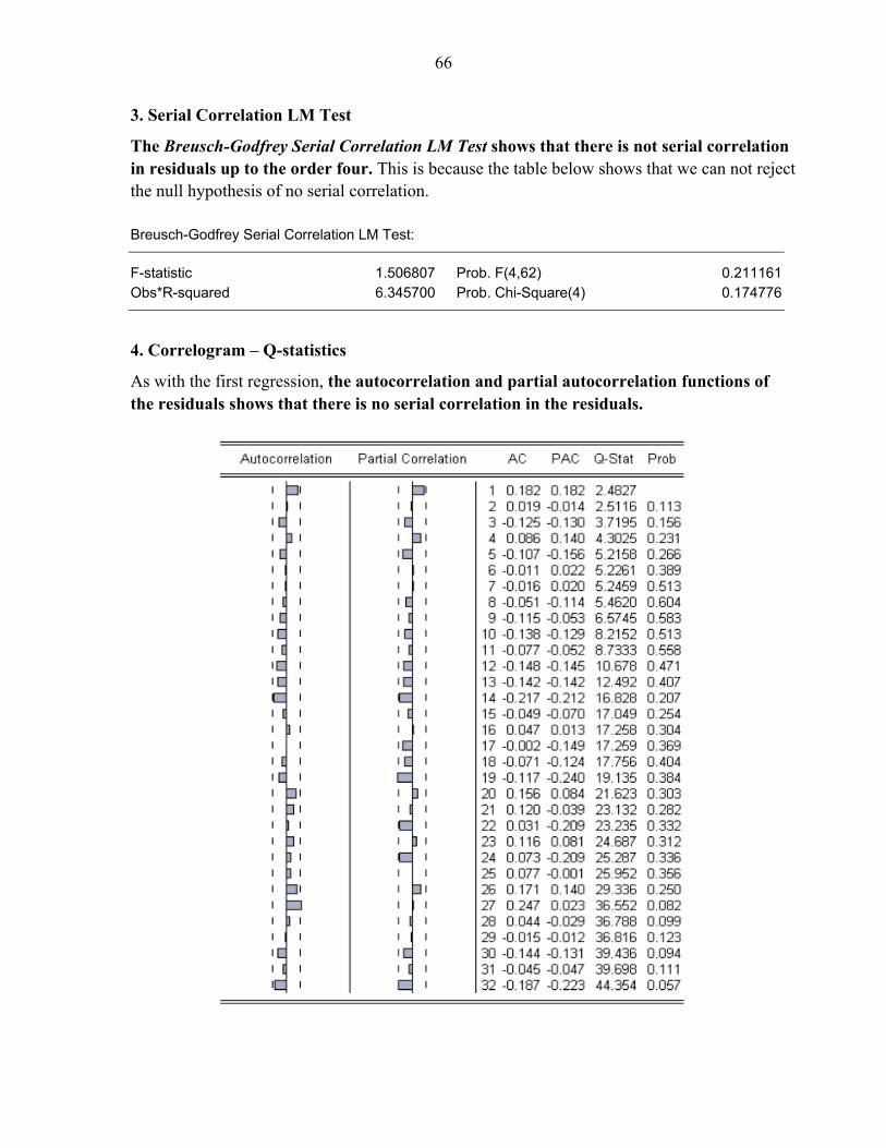
66
3. Serial Correlation LM Test
The Breusch-Godfrey Serial Correlation LM Test shows that there is not serial correlation in residuals up to the order four. This is because the table below shows that we can not reject the null hypothesis of no serial correlation. Breusch-Godfrey Serial Correlation LM Test:
F-statistic 1.506807 Prob. F(4,62) 0.211161Obs*R-squared 6.345700 Prob. Chi-Square(4) 0.174776
4. Correlogram – Q-statistics
As with the first regression, the autocorrelation and partial autocorrelation functions of the residuals shows that there is no serial correlation in the residuals.
67
V. LONG-TERM MANAGEMENT OF HYDROCARBONS RESOURCES1
A. Introduction
1. Driven by high levels of foreign direct investment, the Bolivian natural gas sector has undergone a major transformation in the past decade. Only in the last three years natural gas exports have increased threefold and currently represent almost half of total exports, accounting for about 15 percent of GDP. Domestic consumption of natural gas is still relatively limited, but is expected to grow in coming years.
2. With the recent increase in natural gas royalties, Bolivia’s fiscal accounts have moved towards a high degree of dependency on hydrocarbons-based revenue. Hydrocarbons-related receipts (11 percent of GDP) represent about one-third of public-sector revenue, up sharply from a few years ago. While the rise in export volumes and the energy price environment have played a role, most of the increase in hydrocarbons-based revenue has stemmed from changes in the legal framework for the sector. The Hydrocarbons Law of 2005 and the Nationalization Decree of 2006 have resulted in a much higher government take. Since May 2007, under the new operating contracts with foreign energy companies, such revenue is collected through Bolivia’s oil company (YPFB ).2
3. The strength in hydrocarbons-based revenue is expected to continue for an extended period given the level of reserves and expected additional investments in production in the medium term. This is predicated on Bolivia’s energy-importing neighbors’ interest in maintaining the level of natural gas purchases (Brazil) and/or raising them significantly to address emerging energy bottlenecks (Argentina). Moreover, while production is expected to increase, the information on reserves indicates that Bolivia can count on this resource for the next 50-60 years, depending on the expansion of domestic consumption and the continuation of exploration activities.
4. Accordingly, the availability of hydrocarbons resources poses policy issues not only for the short/medium term3 but also for the long term. In particular, given the magnitude of the proven and probable reserves of natural gas, and the expected production path in the long run, it is important to design a long-term fiscal strategy for the optimal management of these resources. Such a strategy should be consistent with a sustainable use of hydrocarbons resources over a well-defined time horizon, striking an appropriate balance 1 Prepared by Mario Mansilla. 2 Royalties on natural gas production increased from 18 percent to 50 percent. Under the new operating contracts recently put in place, revenue after royalties is subject to a distribution between YPFB and the service operators, depending on an agreed schedule for each gas field, which depends mainly on investment costs. In addition operating companies are subject to the corporate income tax. 3 See Chapter I on Dutch disease issues in this volume.
68
between current public policy objectives (notably, poverty reduction) and intergenerational equity considerations.
5. This Chapter discusses possible strategies for the long-term management of hydrocarbons resources. Based on an assessment of the outlook for the production and prices of natural gas and crude oil, we derive alternative fiscal spending paths with different degrees of sustainability. Such spending paths could be used by the authorities to calibrate fiscal spending in a way that does not deplete the resources, or does so in a gradual manner, allowing future generations to benefit from the country’s energy wealth. The remainder of the Chapter is organized as follows: section B describes briefly the analytical principles underlying the identified strategies; section C presents the main results of the baseline estimates and some sensitivity calculations; and section D concludes.
B. Analytical Underpinnings
6. As other countries with large endowments of natural resources, Bolivia is confronted with the challenge of managing the revenues derived from those resources in a sustainable manner. An optimal long-term fiscal strategy needs to both plan for cyclical swings and incorporate decisions regarding the life span for resource utilization. A fiscal framework that explicitly spells out such decisions has the advantage of minimizing the possibility of drastic policy reversals and their attendant adverse social consequences. Therefore, Bolivia’s fiscal policy should aim at an appropriately calibrated use of energy wealth over time.
7. The specification of long-term fiscal policy paths is underpinned by a partial equilibrium model. In such a model, the government would set its expenditure levels so as to maximize a social welfare function, on a permanent basis, subject to an intertemporal budget constraint and a transversality condition, as follows:4
0)1(..
)(max
1
=−−+⋅+=
⋅
+∞→
−
∞
=
−∑
sts
ttttt
tss
ts
BimlZTGBrBts
GUβ
Where, G represents the level of primary government expenditure, U(.) is a well-behaved social welfare function andβ is the intertemporal discount factor. B represents the stock of debt while T and Z are non-hydrocarbons and hydrocarbons revenue, respectively. Assuming β (1+r) = 1, the optimal solution is a constant level of G: 4 This analysis is based on Barnett and Ossowski (2003).
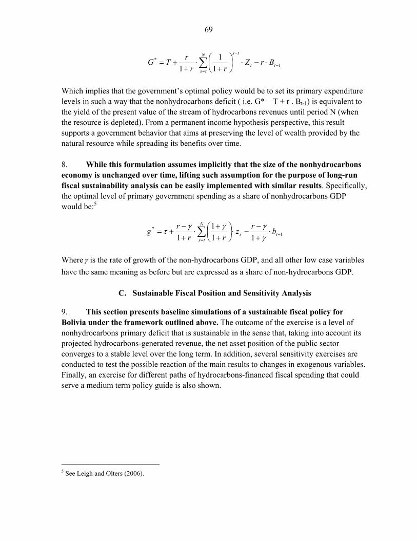
69
∑=
−
−
⋅−⋅⎟⎠⎞
⎜⎝⎛+
⋅+
+=N
tstt
ts
BrZrr
rTG 1*
11
1
Which implies that the government’s optimal policy would be to set its primary expenditure levels in such a way that the nonhydrocarbons deficit ( i.e. G* – T + r . Bt-1) is equivalent to the yield of the present value of the stream of hydrocarbons revenues until period N (when the resource is depleted). From a permanent income hypothesis perspective, this result supports a government behavior that aims at preserving the level of wealth provided by the natural resource while spreading its benefits over time. 8. While this formulation assumes implicitly that the size of the nonhydrocarbons economy is unchanged over time, lifting such assumption for the purpose of long-run fiscal sustainability analysis can be easily implemented with similar results. Specifically, the optimal level of primary government spending as a share of nonhydrocarbons GDP would be:5
∑=
−⋅+−
−⋅⎟⎠⎞
⎜⎝⎛
++
⋅+−
+=N
tsts brz
rrrg 1
*
111
1 γγγγτ
Whereγ is the rate of growth of the non-hydrocarbons GDP, and all other low case variables have the same meaning as before but are expressed as a share of non-hydrocarbons GDP.
C. Sustainable Fiscal Position and Sensitivity Analysis
9. This section presents baseline simulations of a sustainable fiscal policy for Bolivia under the framework outlined above. The outcome of the exercise is a level of nonhydrocarbons primary deficit that is sustainable in the sense that, taking into account its projected hydrocarbons-generated revenue, the net asset position of the public sector converges to a stable level over the long term. In addition, several sensitivity exercises are conducted to test the possible reaction of the main results to changes in exogenous variables. Finally, an exercise for different paths of hydrocarbons-financed fiscal spending that could serve a medium term policy guide is also shown.
5 See Leigh and Olters (2006).
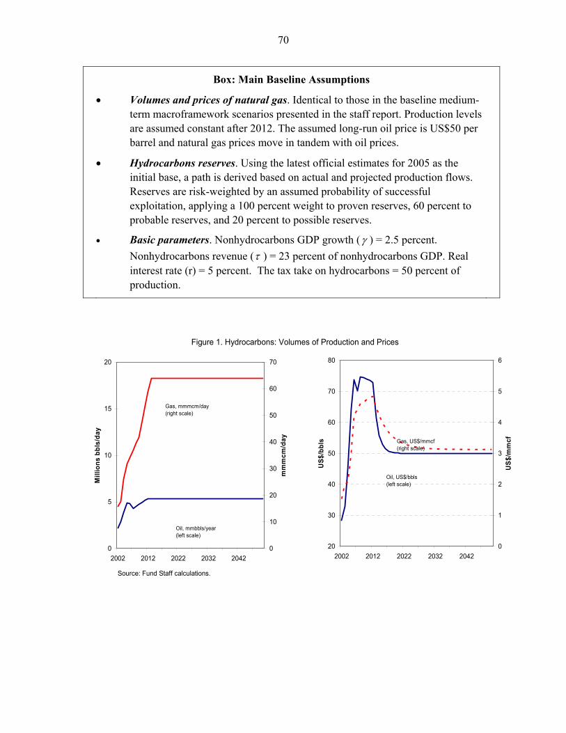
70
Box: Main Baseline Assumptions
• Volumes and prices of natural gas. Identical to those in the baseline medium-term macroframework scenarios presented in the staff report. Production levels are assumed constant after 2012. The assumed long-run oil price is US$50 per barrel and natural gas prices move in tandem with oil prices.
• Hydrocarbons reserves. Using the latest official estimates for 2005 as the initial base, a path is derived based on actual and projected production flows. Reserves are risk-weighted by an assumed probability of successful exploitation, applying a 100 percent weight to proven reserves, 60 percent to probable reserves, and 20 percent to possible reserves.
• Basic parameters. Nonhydrocarbons GDP growth (γ ) = 2.5 percent. Nonhydrocarbons revenue (τ ) = 23 percent of nonhydrocarbons GDP. Real interest rate (r) = 5 percent. The tax take on hydrocarbons = 50 percent of production.
Figure 1. Hydrocarbons: Volumes of Production and Prices
Source: Fund Staff calculations.
0
5
10
15
20
2002 2012 2022 2032 2042
Mill
ions
bbl
s/da
y
0
10
20
30
40
50
60
70
mm
mcm
/day
Gas, mmmcm/day (right scale)
Oil, mmbbls/year (left scale)
20
30
40
50
60
70
80
2002 2012 2022 2032 2042
US$
/bbl
s
0
1
2
3
4
5
6
US$
/mm
cfGas, US$/mmcf (right scale)
Oil, US$/bbls (left scale)
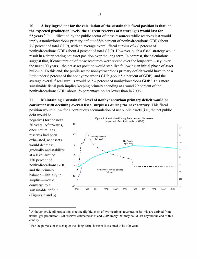
71
-15
-10
-5
0
5
10
15
2002 2012 2022 2032 2042 2052 2062 2072 2082 2092 2102-350
-250
-150
-50
50
150
250
350
450
Primary balance (left axis)
Non-hydroc. primary balance(left axis)
Figure 2. Sustainable Primary Balances and Net Assets(In percent of nonhydrocarbons GDP)
Net Assets(right axis)
10. A key ingredient for the calculation of the sustainable fiscal position is that, at the expected production levels, the current reserves of natural gas would last for 52 years.6 Full utilization by the public sector of these resources while reserves last would imply a nonhydrocarbons primary deficit of 8¼ percent of nonhydrocarbons GDP (about 7½ percent of total GDP), with an average overall fiscal surplus of 4½ percent of nonhydrocarbons GDP (about 4 percent of total GDP). However, such a fiscal strategy would result in a deteriorating net asset position over the long term. In contrast, the calculations suggest that, if consumption of those resources were spread over the long-term—say, over the next 100 years—the net asset position would stabilize following an initial phase of asset build-up. To this end, the public sector nonhydrocarbons primary deficit would have to be a little under 6 percent of the nonhydrocarbons GDP (about 5¼ percent of GDP), and the average overall fiscal surplus would be 5¼ percent of nonhydrocarbons GDP.7 This more sustainable fiscal path implies keeping primary spending at around 29 percent of the nonhydrocarbons GDP, about 1½ percentage points lower than in 2006.
11. Maintaining a sustainable level of nonhydrocarbon primary deficit would be consistent with declining overall fiscal surpluses during the next century. This fiscal position would allow for a continuous accumulation of net public assets (i.e., the net public debt would be negative) for the next 50 years. Afterwards, once natural gas reserves had been exhausted, net assets would decrease gradually and stabilize at a level around 150 percent of nonhydrocarbons GDP, and the primary balance—initially in surplus—would converge to a sustainable deficit. (Figures 2 and 3).
6 Although crude oil production is not negligible, most of hydrocarbons revenues in Bolivia are derived from natural gas production. Oil reserves estimated as at end-2005 imply that they could last beyond the end of this century. 7 For the purpose of this chapter the “long-term” horizon is assumed to be 100 years.
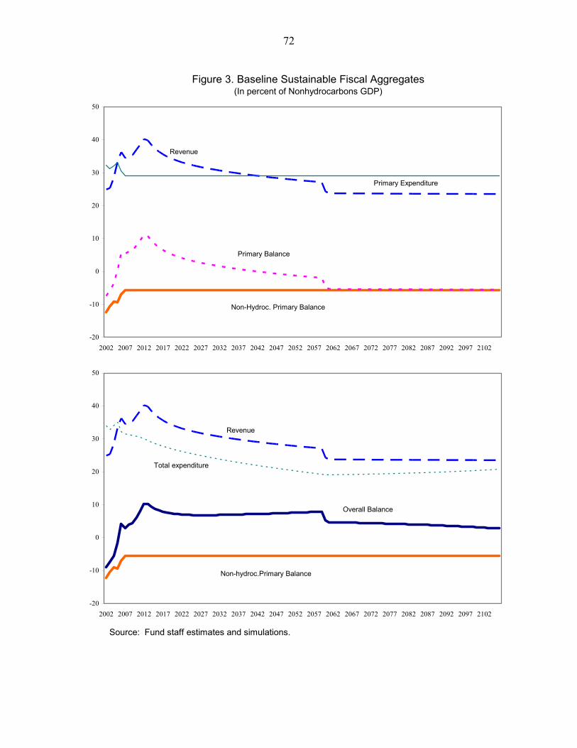
72
Source: Fund staff estimates and simulations.
-20
-10
0
10
20
30
40
50
2002 2007 2012 2017 2022 2027 2032 2037 2042 2047 2052 2057 2062 2067 2072 2077 2082 2087 2092 2097 2102
Revenue
Non-Hydroc. Primary Balance
Primary Balance
Primary Expenditure
-20
-10
0
10
20
30
40
50
2002 2007 2012 2017 2022 2027 2032 2037 2042 2047 2052 2057 2062 2067 2072 2077 2082 2087 2092 2097 2102
Revenue
Non-hydroc.Primary Balance
Overall Balance
Total expenditure
Figure 3. Baseline Sustainable Fiscal Aggregates (In percent of Nonhydrocarbons GDP)
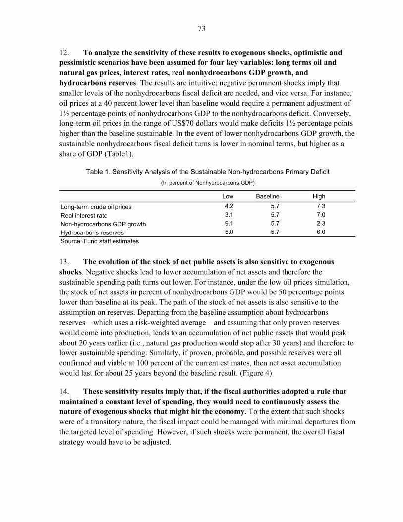
73
12. To analyze the sensitivity of these results to exogenous shocks, optimistic and pessimistic scenarios have been assumed for four key variables: long terms oil and natural gas prices, interest rates, real nonhydrocarbons GDP growth, and hydrocarbons reserves. The results are intuitive: negative permanent shocks imply that smaller levels of the nonhydrocarbons fiscal deficit are needed, and vice versa. For instance, oil prices at a 40 percent lower level than baseline would require a permanent adjustment of 1½ percentage points of nonhydrocarbons GDP to the nonhydrocarbons deficit. Conversely, long-term oil prices in the range of US$70 dollars would make deficits 1½ percentage points higher than the baseline sustainable. In the event of lower nonhydrocarbons GDP growth, the sustainable nonhydrocarbons fiscal deficit turns is lower in nominal terms, but higher as a share of GDP (Table1).
Low Baseline High
Long-term crude oil prices 4.2 5.7 7.3Real interest rate 3.1 5.7 7.0Non-hydrocarbons GDP growth 9.1 5.7 2.3Hydrocarbons reserves 5.0 5.7 6.0Source: Fund staff estimates
Table 1. Sensitivity Analysis of the Sustainable Non-hydrocarbons Primary Deficit(In percent of Nonhydrocarbons GDP)
13. The evolution of the stock of net public assets is also sensitive to exogenous shocks. Negative shocks lead to lower accumulation of net assets and therefore the sustainable spending path turns out lower. For instance, under the low oil prices simulation, the stock of net assets in percent of nonhydrocarbons GDP would be 50 percentage points lower than baseline at its peak. The path of the stock of net assets is also sensitive to the assumption on reserves. Departing from the baseline assumption about hydrocarbons reserves—which uses a risk-weighted average—and assuming that only proven reserves would come into production, leads to an accumulation of net public assets that would peak about 20 years earlier (i.e., natural gas production would stop after 30 years) and therefore to lower sustainable spending. Similarly, if proven, probable, and possible reserves were all confirmed and viable at 100 percent of the current estimates, then net asset accumulation would last for about 25 years beyond the baseline result. (Figure 4)
14. These sensitivity results imply that, if the fiscal authorities adopted a rule that maintained a constant level of spending, they would need to continuously assess the nature of exogenous shocks that might hit the economy. To the extent that such shocks were of a transitory nature, the fiscal impact could be managed with minimal departures from the targeted level of spending. However, if such shocks were permanent, the overall fiscal strategy would have to be adjusted.
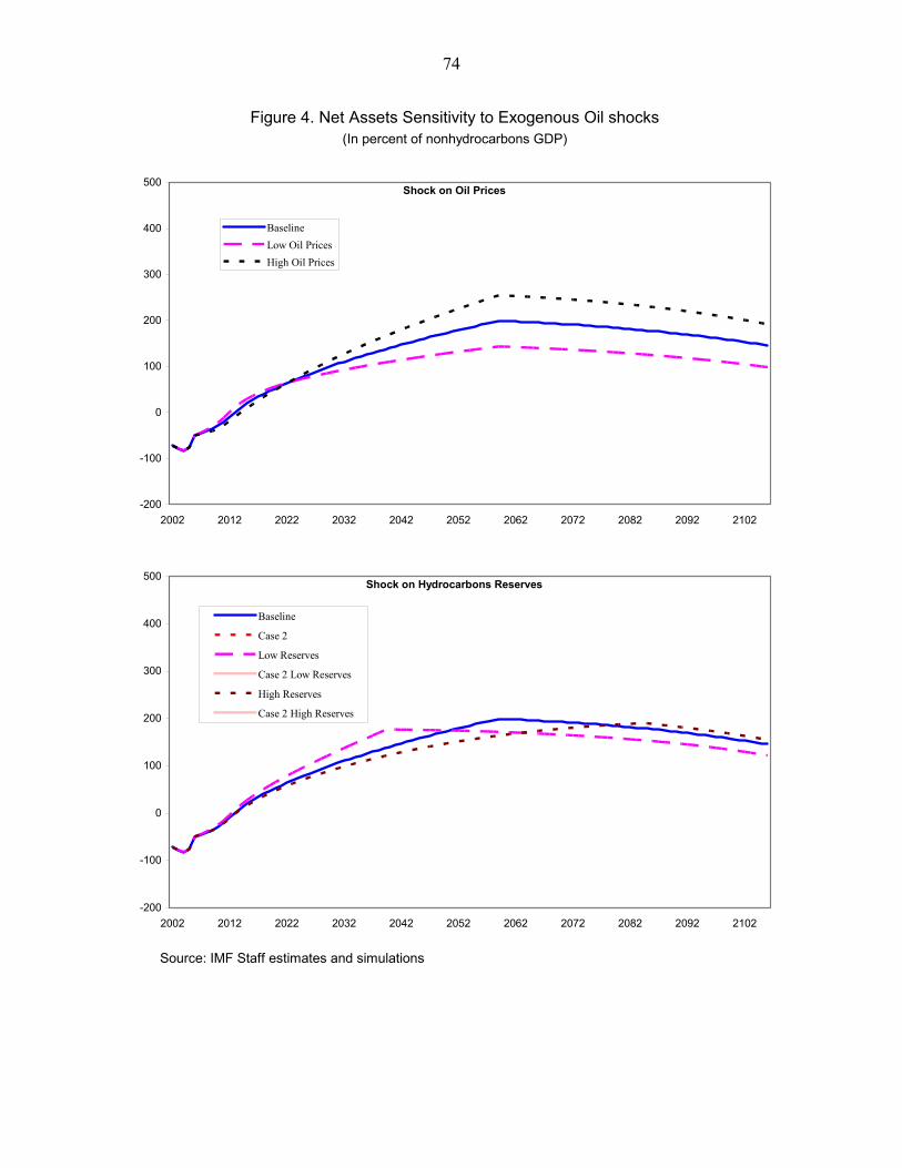
74
Figure 4. Net Assets Sensitivity to Exogenous Oil shocks(In percent of nonhydrocarbons GDP)
Source: IMF Staff estimates and simulations
Shock on Oil Prices
-200
-100
0
100
200
300
400
500
2002 2012 2022 2032 2042 2052 2062 2072 2082 2092 2102
BaselineLow Oil PricesHigh Oil Prices
Shock on Hydrocarbons Reserves
-200
-100
0
100
200
300
400
500
2002 2012 2022 2032 2042 2052 2062 2072 2082 2092 2102
Baseline
Case 2
Low Reserves
Case 2 Low Reserves
High Reserves
Case 2 High Reserves
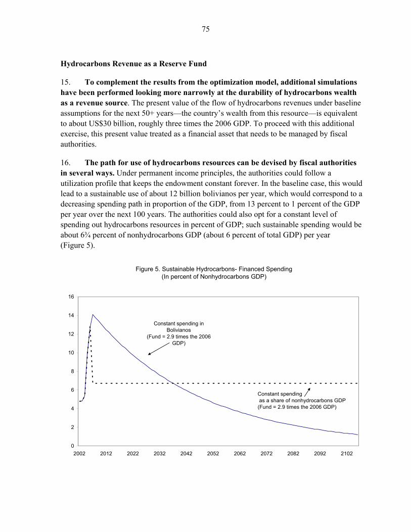
75
Hydrocarbons Revenue as a Reserve Fund
15. To complement the results from the optimization model, additional simulations have been performed looking more narrowly at the durability of hydrocarbons wealth as a revenue source. The present value of the flow of hydrocarbons revenues under baseline assumptions for the next 50+ years—the country’s wealth from this resource—is equivalent to about US$30 billion, roughly three times the 2006 GDP. To proceed with this additional exercise, this present value treated as a financial asset that needs to be managed by fiscal authorities.
16. The path for use of hydrocarbons resources can be devised by fiscal authorities in several ways. Under permanent income principles, the authorities could follow a utilization profile that keeps the endowment constant forever. In the baseline case, this would lead to a sustainable use of about 12 billion bolivianos per year, which would correspond to a decreasing spending path in proportion of the GDP, from 13 percent to 1 percent of the GDP per year over the next 100 years. The authorities could also opt for a constant level of spending out hydrocarbons resources in percent of GDP; such sustainable spending would be about 6¾ percent of nonhydrocarbons GDP (about 6 percent of total GDP) per year (Figure 5).
0
2
4
6
8
10
12
14
16
2002 2012 2022 2032 2042 2052 2062 2072 2082 2092 2102
Constant spending in Bolivianos
(Fund = 2.9 times the 2006 GDP)
Constant spending as a share of nonhydrocarbons GDP(Fund = 2.9 times the 2006 GDP)
Figure 5. Sustainable Hydrocarbons- Financed Spending(In percent of Nonhydrocarbons GDP)
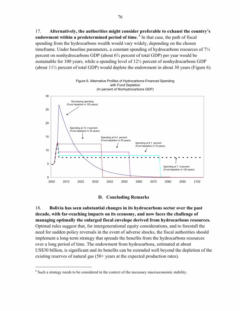
76
17. Alternatively, the authorities might consider preferable to exhaust the country’s endowment within a predetermined period of time. 8 In that case, the path of fiscal spending from the hydrocarbons wealth would vary widely, depending on the chosen timeframe. Under baseline parameters, a constant spending of hydrocarbons resources of 7¼ percent on nonhydrocarbons GDP (about 6¾ percent of total GDP) per year would be sustainable for 100 years, while a spending level of 12½ percent of nonhydrocarbons GDP (about 11½ percent of total GDP) would deplete the endowment in about 30 years (Figure 6).
0
5
10
15
20
25
30
2002 2012 2022 2032 2042 2052 2062 2072 2082 2092 2102
Decreasing spending (Fund depletion in 100 years)
Spending at 9.4 percent (Fund depletion in 50 years)
Figure 6. Alternative Profiles of Hydrocarbons-Financed Spendingwith Fund Depletion
(In percent of Nonhydrocarbons GDP)
Spending at 12 .4 percent (Fund depletion in 30 years)
Spending at 8.1 percent (Fund depletion in 70 years)
Spending at 7 .3 percent (Fund depletion in 100 years)
D. Concluding Remarks
18. Bolivia has seen substantial changes in its hydrocarbons sector over the past decade, with far-reaching impacts on its economy, and now faces the challenge of managing optimally the enlarged fiscal envelope derived from hydrocarbons resources. Optimal rules suggest that, for intergenerational equity considerations, and to forestall the need for sudden policy reversals in the event of adverse shocks, the fiscal authorities should implement a long-term strategy that spreads the benefits from the hydrocarbons resources over a long period of time. The endowment from hydrocarbons, estimated at about US$30 billion, is significant and its benefits can be extended well beyond the depletion of the existing reserves of natural gas (50+ years at the expected production rates).
8 Such a strategy needs to be considered in the context of the necessary macroeconomic stability.
77
19. Baseline estimations suggest that the use of hydrocarbons resources implied by the current and projected fiscal stance are broadly sustainable from an intergenerational equity perspective. Specifically, if the national objective were to use hydrocarbons resources for about 100 years, the 2006 nonhydrocarbons deficit would be about right. However, a reduction of 1–1.5 percent of GDP in public sector spending compared to 2006 would be required to put the use of hydrocarbons on a permanently sustainable level. The fiscal authorities could take advantage of the current environment to set long term goals for the use of the country’s endowment and adopt mechanisms to enforce and manage the resources optimally. International experience in this area points to the establishment of stabilization funds and fiscal rules that help guide the overall fiscal policy, especially give then potential for permanent adverse exogenous shocks to the economy.9
9 See Davis et.al. (2003) for the operational implications and effectiveness of nonrenewable resource funds. Capra and Evia (2007) discuss possible scenarios for the implementation of a reserve fund in Bolivia.
78
References
Barnett, Steven, and Rolando Ossowski, 2003, “Operational Aspects of Fiscal Policy in Oil-Producing Countries,” in Fiscal Policy Formulation and Implementation in Oil-Producing Countries, ed. by Jeffrey Davis, Rolando Ossowski, and Annalisa Fedelino (Washington: International Monetary Fund), pp.45–81.
Capra, Khaterina, and Pablo Evia, 2007, “Fondo de Estabilizacion,” Revista Analisis
Economico, Vol. 22. (Bolivia: Unidad de Analisis de Politicas Sociales y Economicas), pp. 59–74.
Catena, Marcelo, and Fernando Navajas, 2006, “Oil and debt Windfalls and Fiscal Dynamics
in Bolivia,” Economic and Social Study Series RE1-06-003 (Washington: Inter-American Development Bank).
Davis, Jeffrey, Rolando Ossowski, James Daniel, and Steven Barnett, 2003, “Stabilization
and Savings Funds for Nonrenewable Resources: Experience and Fiscal Policy Implications,” in Fiscal Policy Formulation and Implementation in Oil-Producing Countries, ed. by Jeffrey Davis, Rolando Ossowski, and Annalisa Fedelino (Washington: International Monetary Fund), pp.273–315.
De Carvalho Filho, Irineu, 2007, “Medium-Term Fiscal Sustainability in Trinidad and
Tobago,” IMF Staff Country Report 07/8 (Washington: International Monetary Fund), pp.2–14.
Leigh, Daniel, and Jan-Peter Olters, 2006, “Natural Resource Depletion, Habit Formation,
and Sustainable Fiscal Policy: Lessons from Gabon,” IMF Staff Country Report 06/232 (Washington: International Monetary Fund), pp.4–21.
Pivovarsky, Alexander, 2006, “Assessing Fiscal Performance under Dollarization and Policy
Challenges of Securing Long-Run Debt Sustainability,” IMF Staff Country Report 06/103 (Washington: International Monetary Fund), pp.27–42.
Velculescu, Delia, and Saqib Rizavi, 2005, “Trinidad and Tobago: The Energy Boom and
Proposals for a Sustainable Fiscal Policy,” IMF Working Paper WP/05/197 (Washington: International Monetary Fund).