1

Research Department of Borsa İstanbul

Working Paper Series No.18

March, 2014

Bond Markets, Stock Markets and Exchange Rates:

A Dynamic Relationship

Süleyman Hilmi Kal

Central Bank of the

Republic of Turkey

Ferhat Arslaner

Borsa İstanbul

Nuran Arslaner

Central Bank of the

Republic of Turkey

Bond Markets, Stock Markets and Exchange Rates:

A Dynamic Relationship

Süleyman Hilmi Kal

Phd, Economist, the Central Bank of the Republic of Turkey

Istiklal Cad. 10 Ulus Ankara 06100 Turkey

E-mail: suleyman.kal@tcmb.gov.tr

Tel: +90-312-5075447; Fax: +90-312-5075732

Ferhat Arslaner

Phd, Chief Economist/Specialist, Borsa Istanbul

Tuncay Artun Cad. Emirgan Istanbul 34467 Turkey

E-mail: ferhat.arslaner@borsaistanbul.com

Tel: +90-212-2982215; Fax: +90-212-2982189

Nuran Arslaner

Phd, Advisor to the President, the Central Bank of the Republic of Turkey

Bankalar Cad. 13 Karakoy Istanbul 34420 Turkey

E-mail: nuran.arslaner@tcmb.gov.tr

Tel: +90-212-2518000; Fax: +90-212-2529367

Abstract

The paper is an investigation concerning whether the deviations of currencies from

their fundamental values affects the relationship between economic fundamentals and

exchange rates. To this end, a version of the sticky price monetary exchange rate model,

which connects the exchange rates to economic fundamentals, is employed. And that model

is extended by adding a two state time varying transition probability Markov regime

switching process in which transition between regimes is linked to the rate of risk-adjusted

excess returns in the currencies. This permits analysis of the transitional dynamics of

exchange rates. Quarterly data of the most active four floating currencies are used in the

model. These currencies are the Australian dollar, the Canadian dollar, the Japanese yen,

and the British pound. The results provide evidence that the Sharpe ratios of debt and

equity investments in the currencies influence the evolution of transitional dynamics of the

exchange rates’ deviation from their fundamental values. As an extension of this result, it

was found that the relationship between economic fundamentals and the nominal exchange

rates are subject to change depending on the overvaluation or undervaluation of the

currencies relative to their fundamental value.

Keywords: Bond Price, Stock Price, Sharpe Ratio, Exchange Rates, Time Series Analysis,

and Markov Switching Model

JEL: C22, E44, G12

Disclaimer: The views expressed are those of the authors and should not be attributed to their institutions.

1. Introduction

The linkages between stock markets, bond markets and exchange rates in this age of integrated

international financial markets is important not only as an academic endeavor, but also because it has

significant implications for investors, who constantly monitor these markets to take advantage of

excess return. Huge quantities of capital flow between the international markets in search of an extra

yield1. This fact has the potential to cause undervaluation or overvaluation of domestic currencies by

pushing them away from their fundamental values. Since the rate of appreciation and depreciation of

the domestic currencies is also an important part of investment strategies in international markets, the

dynamic relationship between exchange rates, stock and bond markets depends on overvaluation and

undervaluation of the domestic currencies. This paper investigates the questions of whether the

relationship between bond markets, stock markets and exchange rates vary depending on overvaluation

and undervaluation of the domestic currencies and whether risk adjusted excess return in bond and

stock markets have any impact on overvaluation and undervaluation of the domestic currencies.

There are two approaches to explain the relationship between stock prices and exchange rates

relationship: First is the traditional approach. This approach (the good market approach) argues that

currency depreciation affects stock prices through export-import channels by making domestically

produced goods cheaper and foreign produced goods more expensive and increases the domestic stock

prices (Solnick, 1987). The second approach is the portfolio adjustment approach (asset approach).

According to this approach, portfolio adjustments occur through foreign capital inflows and outflows

as a result of changes in stock prices. A persistent upward trend in stock prices will attract foreign

capital (inflow) and cause appreciation of the currency, while decrease in stock prices will decrease

stock holders wealth causing a fall in money demand and will lower interest rates causing capital

outflows which will lead to depreciation of the currency.

1 The total value of the world’s financial stock, comprising equity market capitalization and outstanding bonds and loans,

has increased from $175 trillion in 2008 to $212 trillion at the end of 2010 (Roxburgh et al. 2011).

The relationship between exchange rates and interest rates is an area where the different

approaches are deeply rooted and distinctive between economic schools of thought. Under the flexible

prices approach (Classical School), the relationship between the exchange rates and interest rates is

positive. While under the sticky prices approach (Keynesian School), this relationship is negative.

There are also different views for the interest rate-stock price relationship. Higher interest rates

increase the opportunity cost of money, decreasing the return and stock prices of the companies. On the

other hand, lower interest rates do not have the opposite impact on the stock prices. Higher money

supply pushes the interest rates down causing higher inflation ceteris paribus. Higher inflation lowers

the real value of stocks and may reduce the demand for stocks.

In addition to the diversity of opinion about the linkages and relationships between economic

fundamentals among economists, recently available evidence suggests that in the foreign exchange

markets, traders attribute to economic fundamentals such as interest rates and stock prices time varying

importance in valuation of the exchange rates (Cheung et al. 2001). Theoretical justifications supported

by the empirical evidence raised the question that more than one form of relationship may exist

between the exchange rates, interest rates, stock prices, gold prices and also oil prices (Kal et al. 2013).

Therefore Markov-switching autoregressive specifications (MS-AR) have been heavily used in order to

capture regime-switching behavior among them.

Recently, there have been some new studies published which investigate the linkages between

stock markets, bond markets and exchange rates. Andersen et al. (2007) studied how high frequency

US, German, and British stock, bond and exchange rate dynamics were linked to economic

fundamentals. They found that high-frequency stock, bond and exchange rate dynamics are linked to

fundamentals.

Nieh and Li (2001) found that there is no significant long run relationship between exchange

rates and stock prices for G7 countries. In the short run, their findings are mixed.

When Tabak (2006) investigated the relationship between Brazilian stock market and exchange

rates he found that there is no longer a relationship between them.

Phylaktis and Ravazzolo (2005) show that stock prices and FX markets are positively linked

using cointegration and multivariate Granger causality tests for some pacific basin countries.

Using a Markov Switching approach to markets in the East Asian region Flavin et al. (2008)

find that shocks that originate in either equity or FX markets have spillover effects on the other market

during “turbulent” market conditions.

Henry (2009) employs a regime switching MS-EGARCH model in order to investigate the

relationship between short term interest rates and the UK equity market. In the low mean-high

volatility regime, the conditional variance of equity returns responds persistently but symmetrically to

equity return innovations. In high return-low volatility regime, equity volatility responds

asymmetrically and without persistence to shocks to equity returns.

Ning (2010) found significant and positive tail dependence between the foreign exchange

market movements and the stock market in G5 countries (US, UK, Germany, Japan, and France) for

the period pre- and post euro using a copula based approach.

Employing a two regime Markov switching-EGARCH model Walid et al. (2011) found strong

evidence of regime switching behavior in volatility on emerging stock markets in “calm” and

“turbulent” periods. They reveal the presence of two volatility regimes for Hong Kong, Singapore,

Malaysia and Mexico. They also provide strong evidence that the relationship between stock and

foreign exchange markets is regime dependent and stock price volatility responds asymmetrically to

events in the foreign exchange market. Their results show that foreign exchange rate changes have a

significant impact on the probability of transition across regimes.

Ehrmann el al. (2011) studied the international transmission mechanism between stocks, bonds

and exchange rates in US and Euro era. They find that asset prices react strongest to other domestic

asset price shocks, and that there are also substantial international spillovers, both within and across

asset classes.

It does not seem that any studies to date investigate the dynamics of the relationship between

stocks, bonds and exchange rates together and the impact of overvaluation and undervaluation of

exchange rates, due to capital flows induced by high risk adjusted returns in the stock and bond

markets, and on the relationship between exchange rates, stock and bonds. This study will give a new

perspective to the interrelationship between stocks, bonds and exchange rates by releasing one state

limitation and answering the question as to whether the overvaluation and undervaluation of the

domestic currencies has a potential influence on this interrelationship. In other words, the results will

provide additional insight as to whether higher risk adjusted returns in stocks and bonds change the

relationship between exchange rates, stock and bonds through attracting\repulsion of foreign capital

flows and thereby overvaluing or undervaluing the domestic currencies. This approach is unique in its

integration of capital flows to exchange rate, stock and bond dynamics. To achieve this goal, we

employed a two state time varying transition probability. The Markov regime-switching process is

implemented to vector auto regression (MS VAR) between exchange rates, interest rates and stock

index yields. In this model, the transition between the overvalued and undervalued states of the

exchange rates is governed by the risk adjusted excess return of debt and equity markets (the Sharpe

ratio). Since the Sharpe ratio is utilized in the international foreign exchange markets as a benchmark

for investments in different currencies, we used it as a proxy to measure the capital flows and their

direct impact on the overvaluation and undervaluation of the exchange rates and the indirect impact on

the relationship between exchange rates, interest rates and stock market yields. This model is

implemented quarterly in the dollar exchange rates of the most active four currencies between 1973

and 2010: the AUD, the CAD, the JPY and the GBP.

Our results provide further evidence that the relationship between special exchange rates,

interest rates and stock index yields are time varying. This peculiarity is particularly obvious in the first

equation (exchange rate) of the MS VAR system. The time varying dynamic manifests itself as

statistically significant and insignificant. We also found that the Sharpe ratios of debt and equity

markets have meaningful influence on overvaluation and undervaluation, so the dynamics of exchange

rate, interest rates and stock index yields.

The rest of the paper is organized as follows: Section 2 explains the Markov Switching models

and details the specifications of our models. Section 3 and 4 discuss the data, estimation and the

adequacy of the MS-VAR model used in this paper. Section 5 presents and interprets the empirical

results obtained. Section 6 summarizes and concludes the paper.

2. The Model

Although Quandt (1958), and Godlfeld and Quandt (1973) are the first economists who utilized the

Markov regime switching models in econometrics, it is only after Hamilton’s (1990) (that) Markov

models found their way into economic literature. Implementation of the Markov process to vector auto

regression model was pioneered by Krolzig (1997). This innovative approach enhances modeling

multivariate representation of related models to non-linear framework.

In the Markov process it is assumed that the observed changes of a dependent variable ( )

between two consecutive periods are a random draw from different normal distributions with means

and standard deviations. These distributions are called regimes (states). The number of states may vary

depending on the situation. State (regime) variables ( ) determine the distribution of each period. In

this paper, we utilized a two state Markovian process in which, during State Zero ( =0) the observed

changes are a random draw from ) distribution and during State One ( ts =1)

the observed change is a random draw from ). The unobserved state variable

evolves following a Markov chain.

Since the mean and the variance of yt depend on the state, the density of yt is conditional on st

and is formulated as follows:

)2

)y(exp(

2

1)sy(

2

st-ttt

st

if

(1)

Markovian switching depends only on the previous state and the probability of switching from

one state to another state is called a transition probability. For instance, switching from State (t-1)j to

State (t) is shown by the following equation:

ijttttt pjsisPksjsisP }{,...},{ 121 (2)

In a two-state time varying transition switching model probabilities are given as:

11

11111

11

exp1

exp);,1/1(

t

ttttt

x

xxssPp (3)

11

11111

01

exp1

exp1);,1/0(

t

ttttt

x

xxssPp (4)

01

01011

00

exp1

exp);,0/0(

t

ttttt

x

xxssPp (5)

01

01011

10

exp1

exp1);,0/1(

t

ttttt

x

xxssPp (6)

The transition probabilities are collected in a Γ, (22), transition matrix:

Γ = and 11

0

j

ijp , 10 ijp (7)

In this particular version of the Markov process, transition probabilities are not constant. As

formulated above, the transition between the overvalued and undervalued state is time varying and that

depends on the vector of which will be explained below.

The MSVAR model of exchange rate, interest rate differential and stock yield differential is

formulated as follows:

tt

e

stt

e

stt

e

st

e

stt smydiece ][][][ 111 (8)

tt

i

stt

i

stt

i

st

i

stt smydidecid ][][][ 111 (9)

tt

p

stt

p

stt

p

st

p

stt smydiecsmyd ][][][ 111 (10)

te = 1

1

t

tt

e

ee (11)

ustr

t iiid (12)

ustr

t smysmysmyd (13)

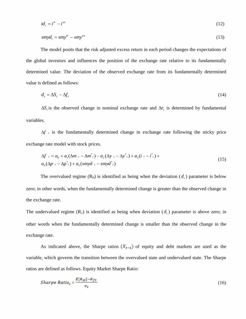
The model posits that the risk adjusted excess return in each period changes the expectations of

the global investors and influences the position of the exchange rate relative to its fundamentally

determined value. The deviation of the observed exchange rate from its fundamentally determined

value is defined as follows:

ttt fSd (14)

tS is the observed change in nominal exchange rate and te is determined by fundamental

variables.

tf is the fundamentally determined change in exchange rate following the sticky price

exchange rate model with stock prices.

)()(

)()()(

*

5

*

4

*

3

*

2

*

10

tttt

ttttttt

smydsmydappa

iiayyammaaf

(15)

The overvalued regime (R0) is identified as being when the deviation ( td ) parameter is below

zero; in other words, when the fundamentally determined change is greater than the observed change in

the exchange rate.

The undervalued regime (R1) is identified as being when deviation ( td ) parameter is above zero; in

other words when the fundamentally determined change is smaller than the observed change in the

exchange rate.

As indicated above, the Sharpe ratios of equity and debt markets are used as the

variable, which governs the transition between the overvalued state and undervalued state. The Sharpe

ratios are defined as follows. Equity Market Sharpe Ratio:

= (16)

][ sRE is the expected rate of return from investments in the domestic debt market or the equity

market is risk-free interest rate and is the standard deviation of expected return of the investment

strategy. Here the standard deviation of the last ten observations is used. Debt Market Sharpe Ratio:

= -E ] + [ ] (17)

The first expression on the right hand side of equation (17), {-E ]}, is the expected

return due to the appreciation of domestic currency and the second expression [ ], is the interest

rate differential between domestic and foreign currencies. As the relative position of the observed

exchange rate to its fundamentally determined value (Equation 10) changes by the global investors'

expectations which are formed by the risk adjusted return (Sharpe ratio), the relationship between

observed exchange rate and economic fundamentals are subject to vary. According to this, in the

overvalued regime (R0) when the Sharpe ratio of debt or equity market increases and if beta (the

coefficient of the xt) is positive then, the likelihood of staying in the overvalued state is formulated by a

logistic function (Equation 3-6) and approaches 1 (one hundred percent) and decreases the probability

of switching to the undervalued state, since some of these probabilities are equal to 1 (Equation 7).

When the exchange rate is in the overvalued state then the relationships between exchange rates,

interest rates and stock yield differentials are defined as the coefficients with the subscript of 0. If the

beta is negative however, the opposite of what is described above will occur.

3. The Data and Estimation

The data set used in this paper covers quarterly observations of four bilateral nominal exchange rates

(price of the US dollar in terms of each currency): the Australian dollar (AUD), the Canadian dollar

(CAD), the Japanese Yen (JPY), and the British Pound (GBP). In addition to this, five macroeconomic

measurements from these four countries and the US are used: money supply, income, inflation rates,

short-term interest rates, and share prices. The data are acquired from the web site of International

Financial Statistics of the IMF and the Bloomberg database.

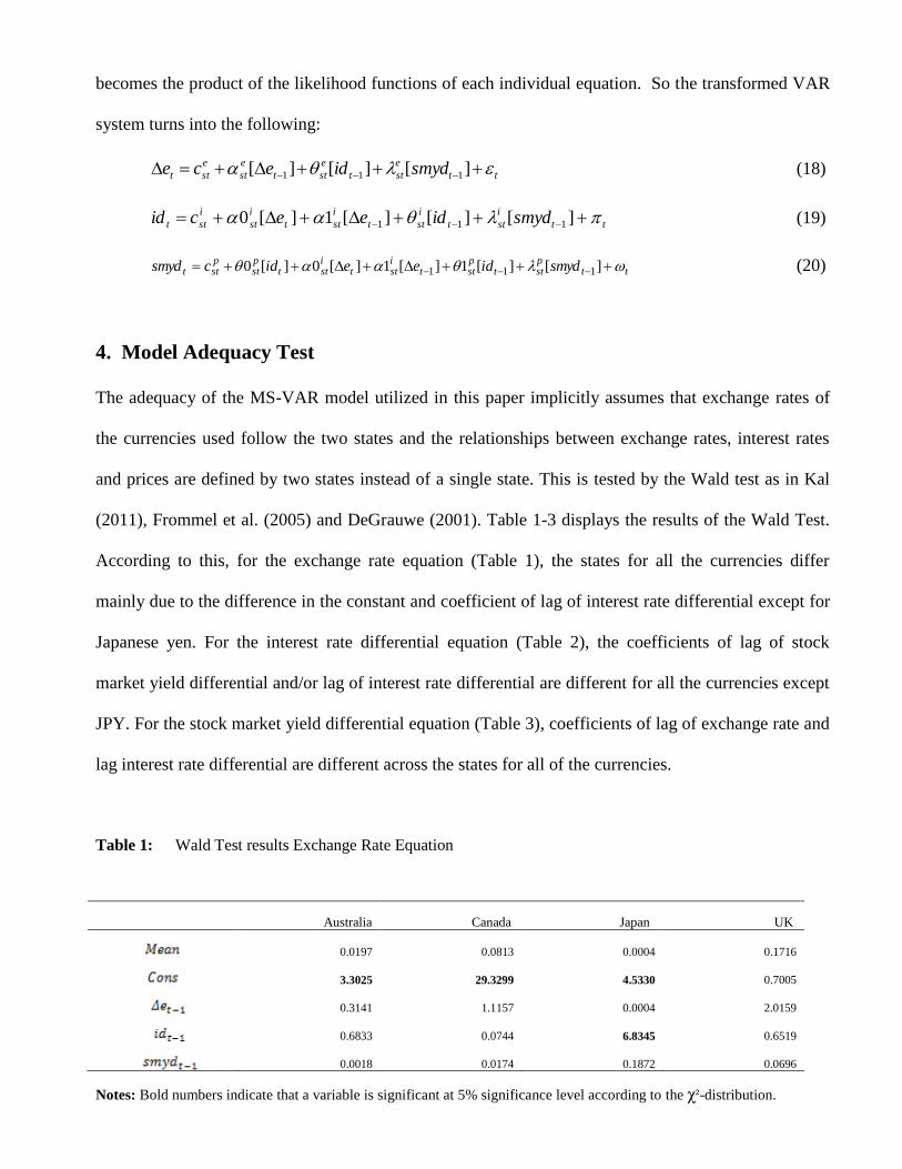
The period covers the 145 end of the period observations of the post Bretton Wood period

beginning with the first quarter of 1972 and ending with the fourth quarter of 2009. As a money supply

measure; the seasonally adjusted M2+CDS is used for Japan, the seasonally adjusted M2 is used for the

US, the seasonally adjusted gross M2 is used for Canada, and the seasonally adjusted M3 is used for

Australia. Since there are some discontinuities for the UK monetary aggregate data in IFS, we acquired

M4 for the UK from the Statistical Data Base of Bank of England. The GDP chain volume with 2002

reference prices is used as income measure for Australia, the GDP chain volume with 2002 prices is

used as an income measure for Canada, nominal GDP is used as an income measure for Japan, GDP

chain volumes with 2000 prices used are used as income measures for the UK and the US. 15 Year

Government Bond Yield is used as the short-term interest rate for all the currencies. The price level in

each economy is measured by CPI. The inflation is calculated by using CPI for each quarter. Share

prices are used as the bases for stock market yield for each currency. The end of quarter share prices is

used for each country.

We used the Expected Maximum Likelihood algorithm developed by Diebold et al. (1994) to

estimate the models. This algorithm depends on maximizing the incomplete log likelihood function by

iterating the expected complete data log likelihood for et, idt, pdt and st conditioned on the data

observed. Using the observed data smoothed state probabilities which can be defined as the

unconditional probability of being in a particular state are calculated. Then the expected complete

likelihood function is found by using the transition probabilities. This step is called the expectation

step. The next step is the maximization step when the expected likelihood function is maximized to

find updated estimates of the parameters. These updated parameter estimates are used to find new

smoothed probabilities, which in turn are used as inputs to expected likelihood function. Finally, this

expected likelihood function is maximized till convergence is reached. However, the above VAR

system - equation (8) to equation (10) - is transformed using a Cholesky decomposition to make the

variance-covariance matrix of the model diagonal. This way, the likelihood function of the model

becomes the product of the likelihood functions of each individual equation. So the transformed VAR

system turns into the following:

tt

e

stt

e

stt

e

st

e

stt smydidece ][][][ 111 (18)

tt

i

stt

i

stt

i

stt

i

st

i

stt smydideecid ][][][1][0 111 (19)

ttpstt

pstt

istt

istt

pst

pstt smydideeidcsmyd ][][1][1][0][0 111 (20)

4. Model Adequacy Test

The adequacy of the MS-VAR model utilized in this paper implicitly assumes that exchange rates of

the currencies used follow the two states and the relationships between exchange rates, interest rates

and prices are defined by two states instead of a single state. This is tested by the Wald test as in Kal

(2011), Frommel et al. (2005) and DeGrauwe (2001). Table 1-3 displays the results of the Wald Test.

According to this, for the exchange rate equation (Table 1), the states for all the currencies differ

mainly due to the difference in the constant and coefficient of lag of interest rate differential except for

Japanese yen. For the interest rate differential equation (Table 2), the coefficients of lag of stock

market yield differential and/or lag of interest rate differential are different for all the currencies except

JPY. For the stock market yield differential equation (Table 3), coefficients of lag of exchange rate and

lag interest rate differential are different across the states for all of the currencies.

Table 1: Wald Test results Exchange Rate Equation

Australia Canada Japan UK

0.0197 0.0813 0.0004 0.1716

3.3025 29.3299 4.5330 0.7005

0.3141 1.1157 0.0004 2.0159

0.6833 0.0744 6.8345 0.6519

0.0018 0.0174 0.1872 0.0696

Notes: Bold numbers indicate that a variable is significant at 5% significance level according to the χ²-distribution.

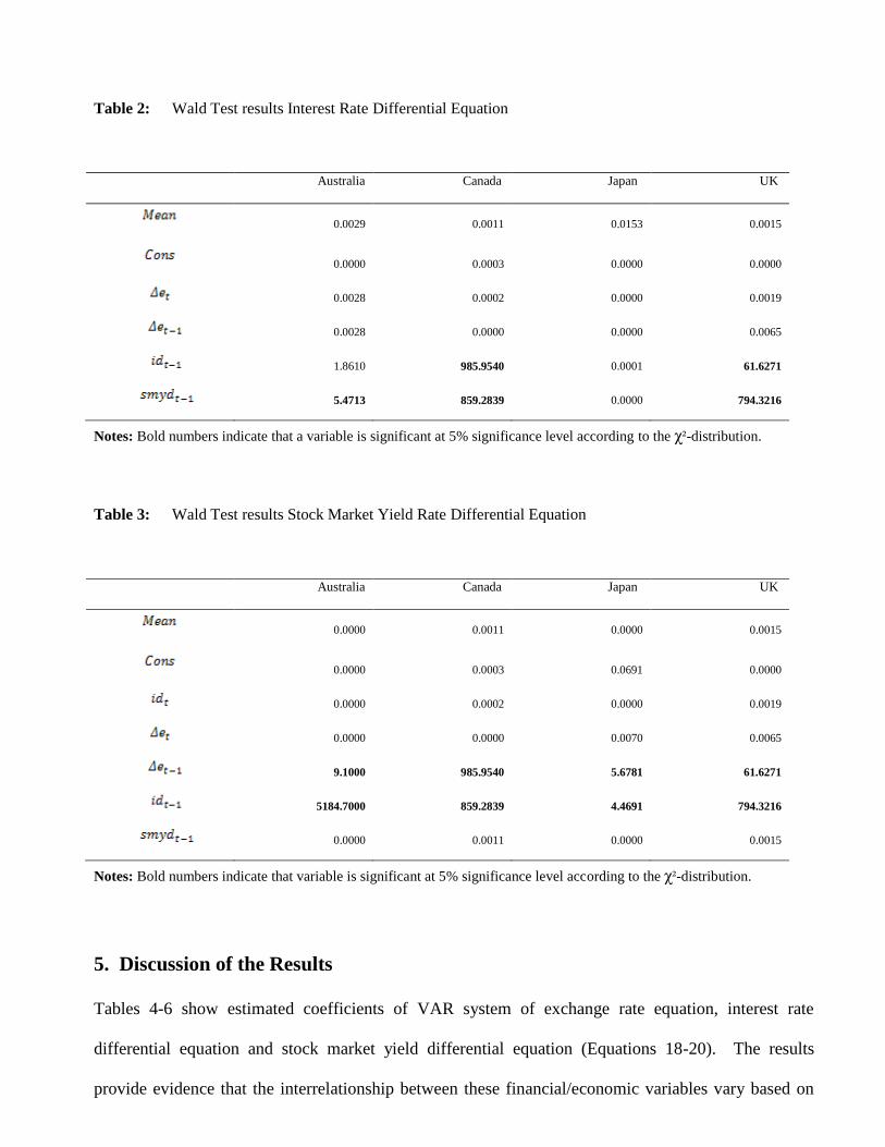
Table 2: Wald Test results Interest Rate Differential Equation

Australia Canada Japan UK

0.0029 0.0011 0.0153 0.0015

0.0000 0.0003 0.0000 0.0000

0.0028 0.0002 0.0000 0.0019

0.0028 0.0000 0.0000 0.0065

1.8610 985.9540 0.0001 61.6271

5.4713 859.2839 0.0000 794.3216

Notes: Bold numbers indicate that a variable is significant at 5% significance level according to the χ²-distribution.

Table 3: Wald Test results Stock Market Yield Rate Differential Equation

Australia Canada Japan UK

0.0000 0.0011 0.0000 0.0015

0.0000 0.0003 0.0691 0.0000

0.0000 0.0002 0.0000 0.0019

0.0000 0.0000 0.0070 0.0065

9.1000 985.9540 5.6781 61.6271

5184.7000 859.2839 4.4691 794.3216

0.0000 0.0011 0.0000 0.0015

Notes: Bold numbers indicate that variable is significant at 5% significance level according to the χ²-distribution.

5. Discussion of the Results

Tables 4-6 show estimated coefficients of VAR system of exchange rate equation, interest rate

differential equation and stock market yield differential equation (Equations 18-20). The results

provide evidence that the interrelationship between these financial/economic variables vary based on

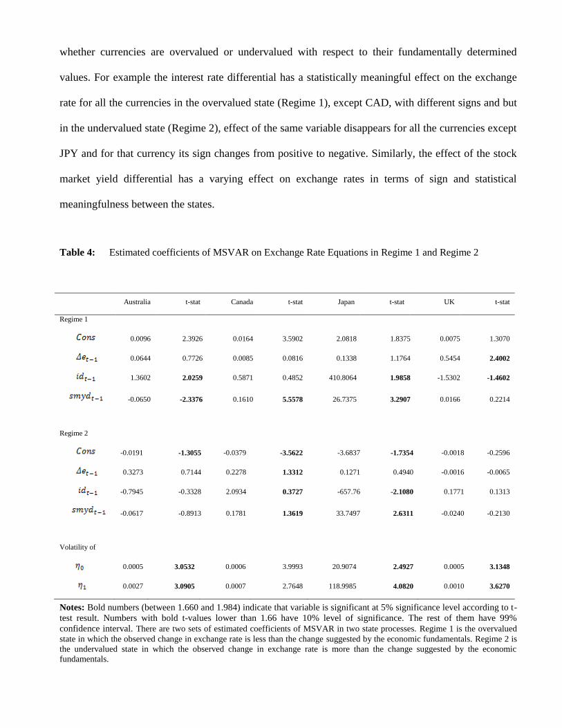
whether currencies are overvalued or undervalued with respect to their fundamentally determined

values. For example the interest rate differential has a statistically meaningful effect on the exchange

rate for all the currencies in the overvalued state (Regime 1), except CAD, with different signs and but

in the undervalued state (Regime 2), effect of the same variable disappears for all the currencies except

JPY and for that currency its sign changes from positive to negative. Similarly, the effect of the stock

market yield differential has a varying effect on exchange rates in terms of sign and statistical

meaningfulness between the states.

Table 4: Estimated coefficients of MSVAR on Exchange Rate Equations in Regime 1 and Regime 2

Australia t-stat Canada t-stat Japan t-stat UK t-stat

Regime 1

0.0096 2.3926 0.0164 3.5902 2.0818 1.8375 0.0075 1.3070

0.0644 0.7726 0.0085 0.0816 0.1338 1.1764 0.5454 2.4002

1.3602 2.0259 0.5871 0.4852 410.8064 1.9858 -1.5302 -1.4602

-0.0650 -2.3376 0.1610 5.5578 26.7375 3.2907 0.0166 0.2214

Regime 2

-0.0191 -1.3055 -0.0379 -3.5622 -3.6837 -1.7354 -0.0018 -0.2596

0.3273 0.7144 0.2278 1.3312 0.1271 0.4940 -0.0016 -0.0065

-0.7945 -0.3328 2.0934 0.3727 -657.76 -2.1080 0.1771 0.1313

-0.0617 -0.8913 0.1781 1.3619 33.7497 2.6311 -0.0240 -0.2130

Volatility of

0.0005 3.0532 0.0006 3.9993 20.9074 2.4927 0.0005 3.1348

0.0027 3.0905 0.0007 2.7648 118.9985 4.0820 0.0010 3.6270

Notes: Bold numbers (between 1.660 and 1.984) indicate that variable is significant at 5% significance level according to t-

test result. Numbers with bold t-values lower than 1.66 have 10% level of significance. The rest of them have 99%

confidence interval. There are two sets of estimated coefficients of MSVAR in two state processes. Regime 1 is the overvalued

state in which the observed change in exchange rate is less than the change suggested by the economic fundamentals. Regime 2 is

the undervalued state in which the observed change in exchange rate is more than the change suggested by the economic

fundamentals.

It is also noteworthy that all the currencies are much more volatile with higher standard

deviations under the overvalued state which also supports the more nuanced relationship between

exchange rates and fundamentals when the currencies are overvalued. This indicates that, during

Regime 1, the overvalued state, the exchange rates become more volatile and the link between

economic fundamentals and exchange rates gets stronger.

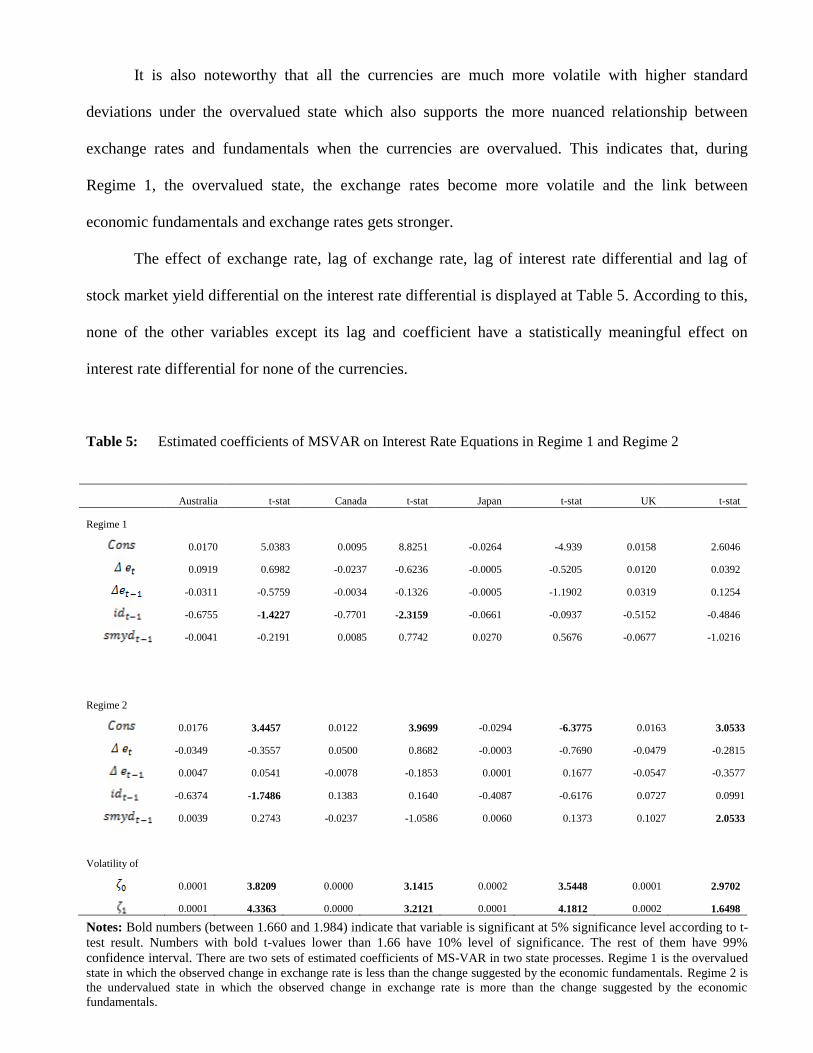
The effect of exchange rate, lag of exchange rate, lag of interest rate differential and lag of

stock market yield differential on the interest rate differential is displayed at Table 5. According to this,

none of the other variables except its lag and coefficient have a statistically meaningful effect on

interest rate differential for none of the currencies.

Table 5: Estimated coefficients of MSVAR on Interest Rate Equations in Regime 1 and Regime 2

Australia t-stat Canada t-stat Japan t-stat UK t-stat

Regime 1

0.0170 5.0383 0.0095 8.8251 -0.0264 -4.939 0.0158 2.6046

0.0919 0.6982 -0.0237 -0.6236 -0.0005 -0.5205 0.0120 0.0392

-0.0311 -0.5759 -0.0034 -0.1326 -0.0005 -1.1902 0.0319 0.1254

-0.6755 -1.4227 -0.7701 -2.3159 -0.0661 -0.0937 -0.5152 -0.4846

-0.0041 -0.2191 0.0085 0.7742 0.0270 0.5676 -0.0677 -1.0216

Regime 2

0.0176 3.4457 0.0122 3.9699 -0.0294 -6.3775 0.0163 3.0533

-0.0349 -0.3557 0.0500 0.8682 -0.0003 -0.7690 -0.0479 -0.2815

0.0047 0.0541 -0.0078 -0.1853 0.0001 0.1677 -0.0547 -0.3577

-0.6374 -1.7486 0.1383 0.1640 -0.4087 -0.6176 0.0727 0.0991

0.0039 0.2743 -0.0237 -1.0586 0.0060 0.1373 0.1027 2.0533

Volatility of

0.0001 3.8209 0.0000 3.1415 0.0002 3.5448 0.0001 2.9702

0.0001 4.3363 0.0000 3.2121 0.0001 4.1812 0.0002 1.6498

Notes: Bold numbers (between 1.660 and 1.984) indicate that variable is significant at 5% significance level according to t-

test result. Numbers with bold t-values lower than 1.66 have 10% level of significance. The rest of them have 99%

confidence interval. There are two sets of estimated coefficients of MS-VAR in two state processes. Regime 1 is the overvalued

state in which the observed change in exchange rate is less than the change suggested by the economic fundamentals. Regime 2 is

the undervalued state in which the observed change in exchange rate is more than the change suggested by the economic

fundamentals.

In Equation 10, the stock market yield differential is explained with the exchange rate, the lag

of exchange rate, the interest rate differential, the lag of interest rate differential and the lag itself. The

results of this equation are shown in Table 6. According to this, in the overvalued state, the interest rate

differential has a negative sign effect on the stock market yield differential for UKP but a positive

effect on CAD, the lag of interest rate differential also has a negative effect on the stock market yield

differential for UKP. Again, in the same state, the exchange rate has a negative effect for the stock

market yield differential for JPY and CAD, and the lag of the same variable has a negative effect for

AUD and a positive effect for CAD on the stock market yield differential. It is important to notice that

at the undervalued state both the interest rate differential and its lag have negative effects for all the

currencies some of which are statistically meaningful though some are not.

Table 6: Estimated coefficients of MSVAR on Stock Market Yield Differential equation in Regime 1 and

Regime 2

Australia t-stat Canada t-stat Japan t-stat UK t-stat

Regime 1

0.0081 0.5672 0.0193 2.0059 -0.0200 -1.0101 0.0034 0.2582

0.7342 0.4163 3.3191 1.5604 -1.0096 -0.3724 -2.9602 1.8760

-0.1545 -0.2543 -0.6736 -2.3970 -0.0069 -2.0526 0.0846 0.2023

-0.5174 -1.7537 0.4189 3.1008 0.0000 0.0062 0.0805 0.1710

0.3523 0.1366 -0.5541 -0.2427 -1.0517 -0.3463 -3.5817 1.7450

-0.5439 -6.3378 -0.3285 -3.8853 -0.3234 -2.5958 -0.6087 4.3980

Regime 2

0.0062 0.3866 -0.0338 -1.6643 -0.0194 -1.0689 -0.0076 0.9430

-0.4499 -0.1737 -2.0697 -0.5770 -1.4233 -0.7496 -2.7332 1.9410

-0.1871 -0.7004 -0.6031 -1.1344 -0.0043 -2.6262 -0.3192 1.2810

-0.2518 -0.6111 0.0763 0.2401 -0.0001 -0.0968 0.2620 1.4175

-0.4254 -0.1815 -3.1937 -0.7434 -3.2574 -1.2685 -2.7551 2.3540

-0.4662 -4.9666 -0.3375 -2.7509 -0.3341 -3.0081 -0.3654 3.2730 Volatility of

0.0106 3.8681 0.005 4.2338 0.0125 4.6697 0.0041 2.8044

0.0090 3.0533 0.0055 3.3445 0.0074 3.4383 0.0037 2.0506

Notes: Bold numbers (between 1.660 and 1.984) indicate that variable is significant at 5% significance level according to t-

test result. Numbers with bold t-values lower than 1.66 have 10% level of significance. The rest of them have 99%

confidence interval. There are two sets of estimated coefficients of MSVAR in two state processes. Regime 1 is the overvalued

state in which the observed change in exchange rate is less than the change suggested by the economic fundamentals. Regime 2 is

the undervalued state in which the observed change in exchange rate is more than the change suggested by the economic

fundamentals.

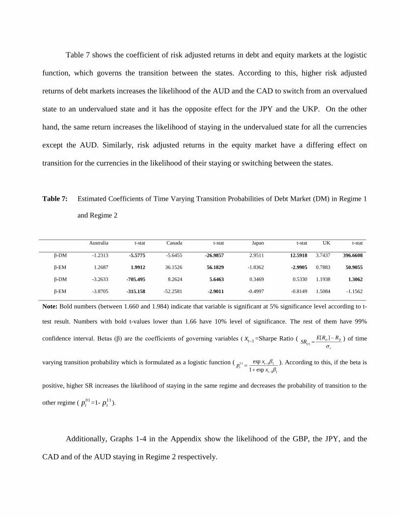
Table 7 shows the coefficient of risk adjusted returns in debt and equity markets at the logistic

function, which governs the transition between the states. According to this, higher risk adjusted

returns of debt markets increases the likelihood of the AUD and the CAD to switch from an overvalued

state to an undervalued state and it has the opposite effect for the JPY and the UKP. On the other

hand, the same return increases the likelihood of staying in the undervalued state for all the currencies

except the AUD. Similarly, risk adjusted returns in the equity market have a differing effect on

transition for the currencies in the likelihood of their staying or switching between the states.

Table 7: Estimated Coefficients of Time Varying Transition Probabilities of Debt Market (DM) in Regime 1

and Regime 2

Australia t-stat Canada t-stat Japan t-stat UK t-stat

β-DM -1.2313 -5.5775 -5.6455 -26.9857 2.9511 12.5918 3.7437 396.6608

β-EM 1.2687 1.9912 36.1526 56.1829 -1.8362 -2.9905 0.7883 50.9055

β-DM -3.2633 -705.495 8.2624 5.6463 0.3469 0.5330 1.1938 1.3062

β-EM -3.8705 -315.158 -52.2581 -2.9011 -0.4997 -0.8149 1.5084 -1.1562

Note: Bold numbers (between 1.660 and 1.984) indicate that variable is significant at 5% significance level according to t-

test result. Numbers with bold t-values lower than 1.66 have 10% level of significance. The rest of them have 99%

confidence interval. Betas (β) are the coefficients of governing variables ( 1tx =Sharpe Ratio (

c

ftct

t

RRESR

][)(

) of time

varying transition probability which is formulated as a logistic function (

11

1111

exp1

exp

t

tt

x

xp ). According to this, if the beta is

positive, higher SR increases the likelihood of staying in the same regime and decreases the probability of transition to the

other regime (01

tp =1-11

tp ).

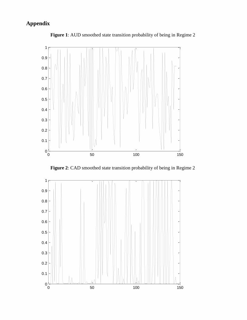
Additionally, Graphs 1-4 in the Appendix show the likelihood of the GBP, the JPY, and the

CAD and of the AUD staying in Regime 2 respectively.

6. Conclusion

In this paper, an analysis of the relationship between exchange rates, interest rates and stock market

yield differentials in the Markovian VAR framework where the states are identified as overvalued

exchange rates and undervalued exchange rates with respect to the fundamentally determined value of

exchange rates. In this model, the transition dynamics between the states are governed by Sharpe ratios

of equity and debt markets of each currency. This structure permits not only an analysis of the

relationship of these important financial series under different exchange rate conditions (overvaluation

and undervaluation) but it also provides a deeper understanding of exchange rate dynamics between

undervaluation and overvaluation depending on risk-adjusted returns of debt and equity markets in

each currency.

The results of this study show that the relationship between exchange rates, interest rate

differentials and stock market yield differentials and their lags as specified in the VAR model are

subject to change as each currency moves above or below their fundamentally determined value. We

also find evidence that the risk-adjusted returns in each currency influence the transition dynamics of

them. That can be attributed to global capital inflows and outflows among other possible sources.

Appendix

Figure 1: AUD smoothed state transition probability of being in Regime 2

0 50 100 1500

0.1

0.2

0.3

0.4

0.5

0.6

0.7

0.8

0.9

1

Figure 2: CAD smoothed state transition probability of being in Regime 2

0 50 100 1500

0.1

0.2

0.3

0.4

0.5

0.6

0.7

0.8

0.9

1

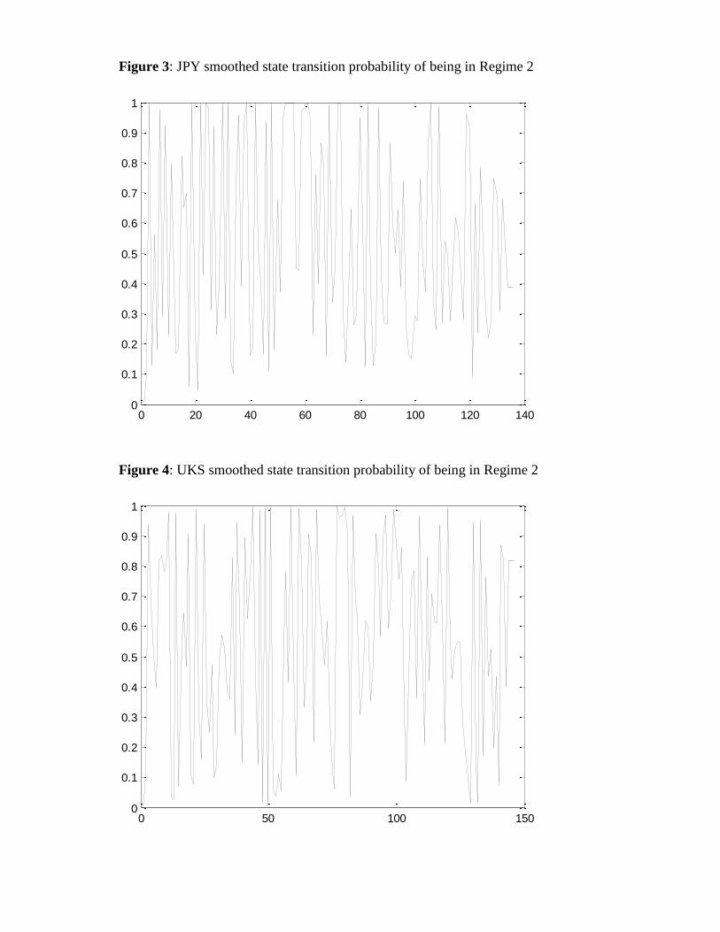
Figure 3: JPY smoothed state transition probability of being in Regime 2

0 20 40 60 80 100 120 1400

0.1

0.2

0.3

0.4

0.5

0.6

0.7

0.8

0.9

1

Figure 4: UKS smoothed state transition probability of being in Regime 2

0 50 100 1500

0.1

0.2

0.3

0.4

0.5

0.6

0.7

0.8

0.9

1

References

[1] Andersen, T. G., T. Bollerslev, F. X. Diebold and C. Vega 2007. “Real-time price discovery in

global stock, bond and foreign exchange markets”, Journal of International Economics 73(2), pp.

251–277.

[2] Cheung, Yin-Wong & Chinn, Menzie David, 2001. “Currency traders and exchange rate dynamics:

a survey of the US market,” Journal of International Money and Finance, Elsevier, vol. 20(4),

pages 439-471, August.

[3] De Grauwe, P. and I. Vansteenkiste 2001. “Exchange Rates and Fundamentals a Non-Linear

Relationship?”, CESifo Working Paper Series No. 577.

[4] Diebold, F. X., Lee, J. H. and Weinbach, G. C. (1994). Regime-switching with time-varying

transition probabilities. In C. Hargreaves (ed.), Nonstationary Time Series Analysis and

Cointegration. Chapter 8. Oxford: Oxford University Press.

[5] Ehrmann M., M. Fratzscher and R. Rigobon 2011. “Stocks, bonds, money markets and exchange

rates: measuring international financial transmission”, Journal of Applied Econometrics 26(6), John

Wiley & Sons, Ltd., pp. 948-974, 09.

[6] Frommel, M., R. MacDonald and L. Menkhoff 2005. “Markov switching regimes in a monetary

exchange rate model”, Economic Modeling, Elsevier, 22(3), pp. 485-502.

[7] Hamilton, James D. 1990. “Analysis of Time Series Subject to Changes in Regime”, Journal of

Econometrics 45, pp. 39-70.

[8] Henry, O.T., 2009. “Regime switching in the relationship between equity returns and short-term

interest rates”, Journal of Banking and Finance, 33, 405–414.

[9] Kal, S. H. 2011. “Global Capital Flows, Time-Varying Fundamentals and Transitional Exchange

Rate Dynamics”, Journal of Forecasting 32(2).

[10] Kal, S. H., F. Arslaner and N. Arslaner 2013. “Gold, Stock Price, Interest Rate and Exchange Rate

Dynamics: An MS VAR Approach” International Research Journal of Finance and Economics,

Issue 107, 8-16.

[11] Kal, S. H., F. Arslaner and N. Arslaner 2013. “Transitional Dynamics of Oil Prices”, International

Research Journal of Finance and Economics, Issue 106, 24-30.

[12] Krolzig, H.-M. 1997. “Markov Switching Vector Autoregressions: Modeling, Statistical Inference

and Application to Business Cycle Analysis: Lecture Notes in Economics and Mathematical

Systems”, 454, Springer-Verlag, Berlin.

[13] Flavin, T.J., Panopoulou, E. and Unalmis, D., 2008. “On the stability of domestic financial market

linkages in the presence of time-varying volatility”, Emerging Markets Review, 9, 280-301.

[14] Nieh, C.-C., C.-F. Lee 2001. “Dynamic relationship between stock prices and exchange rates for G-

7 countries”, The Quarterly Review of Economics and Finance 41(4), pp. 477–490.

[15] Ning, C., 2010. “Dependence structure between the equity market and the foreign market -a copula

approach”, Journal of International Money and Finance, 29, 743-759.

[16] Phylaktis, K. and Ravazzolo, F., 2005. “Stock prices and exchange rate dynamics”, Journal of

International Money and Finance, 24, 1031-1053.

[17] Quandt, Richard E. 1958. “The Estimation of Parameters of Linear Regression System Obeying

Two Separate Regimes”, Journal of the American Statistical Association 55, pp. 873-880.

[18] Roxburgh, C., S. Lund and J. Piotrowski 2011. “Mapping Global Capital Markets 2011” McKinsey

Global Institute Updated Research.

[19] Slink, B. 1987. “Using Financial Prices to Test Exchange Rate Models: A Note”, Journal of

Finance 42, pp. 141-149.

[20] Tabak, B. M. 2006. “The Dynamic Relationship Between Stock Prices And Exchange Rates:

Evidence for Brazil”, International Journal of Theoretical and Applied Finance, World Scientific

Publishing Co. Pte. Ltd., 9(08), pp. 1377-1396.

[21] Walid, C., C. A. Chaker, O. Masood and J. Fry 2011. “Stock market volatility and exchange rates in

emerging countries: A Markov-state switching approach”, Emerging Markets Review, 12, pp. 272-

292.