bond relative value models and term structure of credit ... · within such a fitting framework,...
TRANSCRIPT

- 1 -
Bond Relative Value Models and Term Structure of Credit Spreads:
A Simplified Approach
Kurt Hess
Senior Fellow
Department of Finance
Waikato Management School, University of Waikato,
Hamilton, New Zealand
VERSION 17-Jun-04
Contact details: Kurt Hess, University of Waikato, WMS Department of Finance Private Bag 3105, Hamilton, New Zealand ph. +64 7 838 4196, [email protected]

- 2 -
Bond Relative Value Models and Term Structure of Credit Spreads:
A Simplified Approach
Abstract
Bond relative value models to detect mispriced bonds are widely used in the investment community.
These range from simple yield to maturity comparisons to sophisticated stochastic models. The first
step for many of these models is the determination of reference yield curves. There are numerous
publications on these yield curve fitting approaches with related empirical research yet few actually
document practical implementations for operational purposes. Accordingly, the first part of this
article describes and then illustrates implementation of a number of these benchmarking models.
Within such a fitting framework, bonds subject to credit risk can often not be handled since the
number of bonds of equivalent credit quality is simply too small to derive reliable reference curves.
Here the article proposes a novel approach to parameterize the term structure of credit spread. Its
main benefit are intuitive model parameters that relate to the concept of how market practitioners
like traders and asset manager tend to measure credit risk of fixed income securities.
Many of the models described herein have been implemented in EXCEL/VBA, some of which are
generalized versions of models that have been developed for practical bond relative value research.
The files containing the models can be downloaded from the following website:
http://www.mngt.waikato.ac.nz/kurt/
Keywords: Bond Relative Value Models, Interest Rate Models, Credit Spreads, Yield Curve
Modeling, Excel, VBA

- 3 -
Bond Relative Value Models and Term Structure of Credit Spreads:
A Simplified Approach
1 Introduction
Relative value model to detect indications of potential excess within a universe of fixed
income securities are widely used in the investment community. In the bond markets, relative value
usually refers to the process of comparing returns among fixed income securities but in a wider
sense this definition can be extended to include comparisons with say related equity instruments.
There are two fundamental factors that primarily affect the pricing of fixed income securities. These
are firstly, the prevailing market interest rates and secondly, the specific credit risk of the bond1. This
paper will deal with models that address these two pricing aspects.
With regard to the interest rate factor, there are a number of theoretical models, many of
them versions of seminal work by Vasicek (1977) and Cox, Ingersoll, & Ross (1985) that postulate
an interest rate process as the driving state variable which in turn determines the shape of the yield
curve and thus the pricing of bonds2. Unfortunately, their practical application for bond pricing is
limited. The yield curve shape and dynamics observed can often not be explained with these
approaches as the true stochastic nature of the interest rate process remains elusive. The usual
method is to calibrate such models with observed yield curves as for example in the models of Ho &
Lee (1986) or Heath, Jarrow, & Morton (1992). This in turn requires methods to derive the term
1 Other pricing factors such as taxation and liquidity premia have also been subject to
research but these are typically not considered in models used by market participants. See Bliss
(1997, p.6) or Ioannides (2003, footnote p. 5) for references to some of these studies.
2 Rebonato (1998) describes most of these popular interest rate models in great detail.

- 4 -
structure from traded instruments or contracts such as bonds or interest rate swaps. The first part of
this article will focus on this class of curve fitting models which — though their parameters do not
have an actual economic meaning — have a much greater significance for the market practitioner.
Section 2 characterizes them along the lines proposed by Bliss (1997) and then details how some of
them have been implemented in EXCEL/VBA. Examples include versions of McCulloch (1971;
1975) and Nelson & Siegel (1987) as well as an unnamed simple approach that is a generalized
version of a model tested in a trading environment. While it can be assumed that similar
implementations are applied in industry, they have not been formally documented in the academic
literature. Moreover, Excel/VBA is widely used for financial analysis, i.e. it provides a very popular
platform to present these models.
In the context of pricing fixed income securities, credit risk is usually measured by the so-
called credit spread which measures the difference in yield offered for a risky bond compared to an
equivalent riskless government bond. Ever since the seminal work of Merton (1974) that pioneered
the structural paradigm in credit risk modeling, the nature and dynamics of this term structure of
credit spreads has been subject to substantial research. One puzzling result is that — even after
accounting for possible taxation effects — one finds that expected default and recovery rates on
bonds can explain only a part of the yield premium actually observed3. There is not only an academic
debate as to how to explain the balance but Collin-Dufresne et al. (2001) illustrate that causes of
spread changes are hard to pinpoint, too. Although they use a large number of proxies affecting
credit risk, they fail to explain most of the observed dynamics. They conclude that the dominant
3 See for example Fons (1994). Elton et al.(2001) estimate spread components due to default
risk, taxation with the balance explained as “risk premium for systemic risk”. Duffie & Lando (2001)
model the imperfect, discrete nature of information flowing to investors to account for higher than
expected credit spread observations.

- 5 -
component of credit spread changes are “local supply/demand shocks” not picked up by any of
their proxies.
In the absence of any conclusive models, investor thus again have to rely on appropriate
credit spread fitting models, similar to the ones discussed earlier in this section4. These give market
practitioners like traders, which will generally be aware of such “local supply/demand factors”, a
first indication of potential mispricing. Unfortunately, the basket of comparable bonds of the same
credit quality is often limited and this prevents fitting reliable term structures of credit spreads to the
data. This article thus presents a heuristic fitting method that can be applied in such situations.
Starting point is a certain target credit spread, i.e. the spread which the investor deems appropriate
for the particular bond or group of bonds. This is then complemented by a number of shape
parameters. While the particular target spread is reviewed regularly, e.g. by means of statistical
analysis, the characteristic of the shape parameters is more static and can also be commonly set for a
larger segment of the bond market, for instance for all lower investment grade bonds5. It is not the
ambition of this approach to compete with any of the more advanced fitting methods such as the
ones derived from equilibrium term structure models6 but to simply provide the practitioner a tool
to uncover apparently mispriced bonds in a first instance. The decision process is helped by the
intuitive nature of target credit spread as the main model parameter. The illustrative Excel/VBA
4 Recent developments are new joint estimation techniques as presented in Houweling,
Hoek, & Kleibergen (2001).
5 An investor might decide to define “lower investment grade” bonds as bonds with rating
BBB- up to BBB+
6 e.g. see Anderson et al. (1996, chapter 4, p. 67)

- 6 -
model implementation presented in section 3 uses data for a sample of Swiss domestic industrial
bonds.
2 Bond Relative Value with Yield Curve Fitting Models
As indicated in the introduction, static yield curve fitting models as a basis to detect
mispriced bonds are very much applied in the markets. Examples are Merrill Lynch (2004) daily
Rich/Cheap Reports for countless bond markets and segments. Krippner (2003) p. 2 also lists JP
Morgan, HSBC Bank and UBS Bank as institutions producing bond relative value research based on
yield curve fitting models. Evidence from various studies such as Sercu & Wu (1997) or more
recently Ioannides (2003) indeed suggests that there is justification for applying such models. For
both the Belgian, respectively UK government bond markets, these studies found significant excess
returns for trading strategies based on buying (shortselling) bonds that are classified as undervalued
(overvalued) relative to a particular estimated term structure model.
The following reviews and classifies these models in general which is then followed by
subsections documenting the implementation of three of them.
2.1 Review of Static Term Structure of Interest Models
The term structure of interest, a concept central to economic and financial theory, plays a
key role not just for the pricing of bonds but also any interest rate contingent claim. This section will
focus on the work that has been done in the area of non-probabilistic yield curve modeling. It
follows a framework proposed by Bliss (1997, p. 4) who sees three dimensions to such models or
rather, there are three decisions required to estimate a term structure of interest as the basis for a
bond relative value model: the pricing function, the approximation function and, finally, the
estimation method.

- 7 -
2.1.1 Pricing Function
The most straightforward pricing function is certainly the present value (P) of the bond’s
promised cash flows (C):
( )∑=
−=M
m
mtmrmeCP
1
)( (1)
where M are the number of remaining cash flows numbered 1 to m; ( )mr and ( )mt are the
spot rates, respectively times at which these cash flows will occur. This is, however, not the only
pricing relation used in the markets. The much simpler yield to maturity based bond valuation is still
very much in use by investors. This because the simple yield measure akin to the well-known
internal rate of return is typically the first piece of bond analytics listed by financial data providers
and the media. Some markets like Australia and New Zealand even refrain from quoting fixed
income securities by price but rather by yield to maturity which in turn is used to calculate the actual
settlement price by means of a standardized formula7. A simplified version of such a formula, using
continuously compounded rates and not considering the complexities of time measurement
conventions8, would look like the pricing formula (1) above with constant rate r, no longer
dependent on the time t of the mth cash flow.
Whatever function is chosen, none will in practice exactly price all bonds in a particular
reference basket. An inexact relation for the price Pj of a particular bond needs to be formulated:
7 See appendix 1 for the example of the New Zealand bond market formula as shown in
RBNZ (1997, p. 12)
8 Christie (2003) provides some detailed description of how time measurement conventions
including factors such as national holiday calendars affect bond yield calculations.

- 8 -
( )[ ] jmj mrCfP ε+= , (2)
where the function [ ].f captures all that we assume what determines the price of the bond
and ( )mr is fitted to minimize some function of the random residual term jε . In formulating [ ].f ,
researchers will often add terms (e.g. dummy variables) to the straight present value formula that
attempt to capture effects of frictions in the markets such as tax effects or liquidity premia9. It is,
however, the experience of this author that this is hardly done in operational models because such
factors tend to have less tangible impact on the price of the instrument.
2.1.2 Approximation Function
As a next step, one must decide on the functional form to approximate either the discount
rate function ( )mr , or the discount function ( )md . This is necessary as there are limited numbers of
bonds which requires a way of interpolating the rates, respectively discount function for arbitrary
time horizons. The usual approach is to select an approximating function and then to estimate the
parameters. We mention here just two mainstream methods10, a parsimonious representation defined
by an exponential decay term pioneered by Nelson & Siegel (1987) and Svensson (1994) and cubic
splines introduced to finance by McCulloch (1971; 1975). The most comprehensive comparative
studies of these and other functional forms have been undertaken by Bliss (1997) and Ioannides
(2003). While there are differences between the very many methods, none is disqualified by these
9 See footnote in introduction for references to alternative pricing factors.
10 Bliss (1997, p.6) and Ioannides (2003, p.3) list references to the major classes of such
models.

- 9 -
researchers11 for their goodness of fit. Weaknesses appear more in other aspects, e.g. difficulty to
estimate parameters (see below) or unstable, respectively fluctuating forward rates implied. With
regard to residual based bond relative models there is thus no cause to discount any of them.
2.1.3 Estimation Method
Lastly, the decision on the appropriate estimation technique is a more technical but
nevertheless important issue. The aspect of estimation not only includes the choice of numerical
algorithms for parameter estimation. These are often determined by the type of functions chosen
before. One must also make decisions on error weighting functions and how to handle bid/ask
spreads. Related are data integrity issues. One might define data filters to remove apparently
erroneous data from the set. The tricky aspect remains that in contrast to empirical research with
historical data, the data constellation in an operational trading application is not known beforehand
so output plausibility checks are essential.
2.2 Implementations of Reference Curve Models
Three reference yield curve models are presented in this paper. Firstly, it shows a simple yield to
maturity based benchmarking tool which is illustrated for a basket of Swiss government bonds. Next
there is the JP Morgan Discount Factor Model (JPM), a version of McCulloch’s (1971; 1975) cubic
spline method and, finally, a bond relative value model using an extended Nelson & Siegel (1987)
approach. The latter two models are illustrated with data of the small universe of New Zealand
11 An exception is the Fisher, Nychka, & Zervos (1995) cubic spline which was found to be
“performing poorly” by Bliss (1997, p. 26).

- 10 -
government bonds. The files containing the models can be downloaded from the website
http://www.mngt.waikato.ac.nz/kurt/ .
In following Table 1, the three models are characterized in line with the framework
presented in the previous section. All the models are set up so they can easily be linked to a real time
price data source. Note that some technical complications may arise from the treatment of accrued
interest which depending on market conventions has to be paid upfront by the bond buyer. The
models assume that prices quoted are so-called clean prices, excluding accrued interest. These and
other issues related to bond analytics are discussed in specialized fixed income resources such as
Fabozzi (1999).

- 11 -
Table 1: Model Classification
I II III
Model Yield to Maturity
Benchmarking
JP Morgan Model
Discount Factor Model
Extended
Nelson & Siegel
Pricing function
Simplified price as function
of yield to maturity, i.e. as
in model II/III but
constant )(),( jrmjr =
( )j
M
m
mjtmjrmjj eCP ε+= ∑
=
−
1
,),(,
see formulas 1,2 for explanation of parameters
Approximation
function
Model yield to maturity
term structure as
polynomial
Model discount function as
a polynomial. Version of
(McCulloch, 1971; 1975)
Spot rate modeled with
exponential form as described
in Bliss (1997, p. 11)
Estimation method OLS of yield to maturity
errors (equal weighting).
Corresponding system of
linear equations solved with
LU Decomposition
Press et al. (1992, p. 43)
OLS of price errors (equal
weighting)
Corresponding system of
linear equations solved
Excel built-in LINEST
function.
Duration weighted least
square, minimized with
Generalized Reduced
Gradient (GRG2) nonlinear
optimization code as
implemented in Excel Solver

- 12 -
2.2.1 Simple yield to maturity based benchmarking model
Yield to maturity, also called redemption yield based measures to find relative value in a
universe of bonds is the traditional method still used by many practitioners. As is commonly known,
yield to maturity assumes that an investor holds the bond to maturity and all the bond’s cash flows
are reinvested at the computed yield to maturity. It is found by solving for the interest rate that will
equate the current price to all cash flows from the bond to maturity. In this sense, it is the same as
the internal rate of return (IRR) defined in many finance textbooks in e.g. in Reilly & Brown (1997,
p. 529).
Needless to say that redemption yield based bond analytics has major shortcomings as was
documented many years ago by Schaefer (1977) and also discussed in Anderson et al. (1996, p. 22).
Reinvesting each coupon at the same rate is tantamount to assuming a flat term structure with
identical spot rates for each maturity. If spot rates increase with maturity, yield to maturity will
underestimate the spot rate. Conversely, it overestimates a downward sloping spot-rate curve.
Having noted this, purely for bond relative value purposes, it remains a useful measure with the
necessary caveats. Coupons should firstly be uniform, particularly within a particular maturity range.
Similarly, errors are smaller if market yield levels, including coupon rates are low. There are many
bond market segments that have comparably low liquidity with wide bid/ask spread. Applying an
easier yield to maturity model in these cases is surely more honest because mispricing will also be
detected with this more crude approach.
The implementation of this redemption yield based relative model is stored in the file named
“ConfBenchmark (Feb04).xls”. It is a generalization of a model that has been used for practical
relative value research in the Swiss bond market for a number of years. It was applied to a number
of homogeneous market segments providing information regarding the relative pricing of these
- 13 -
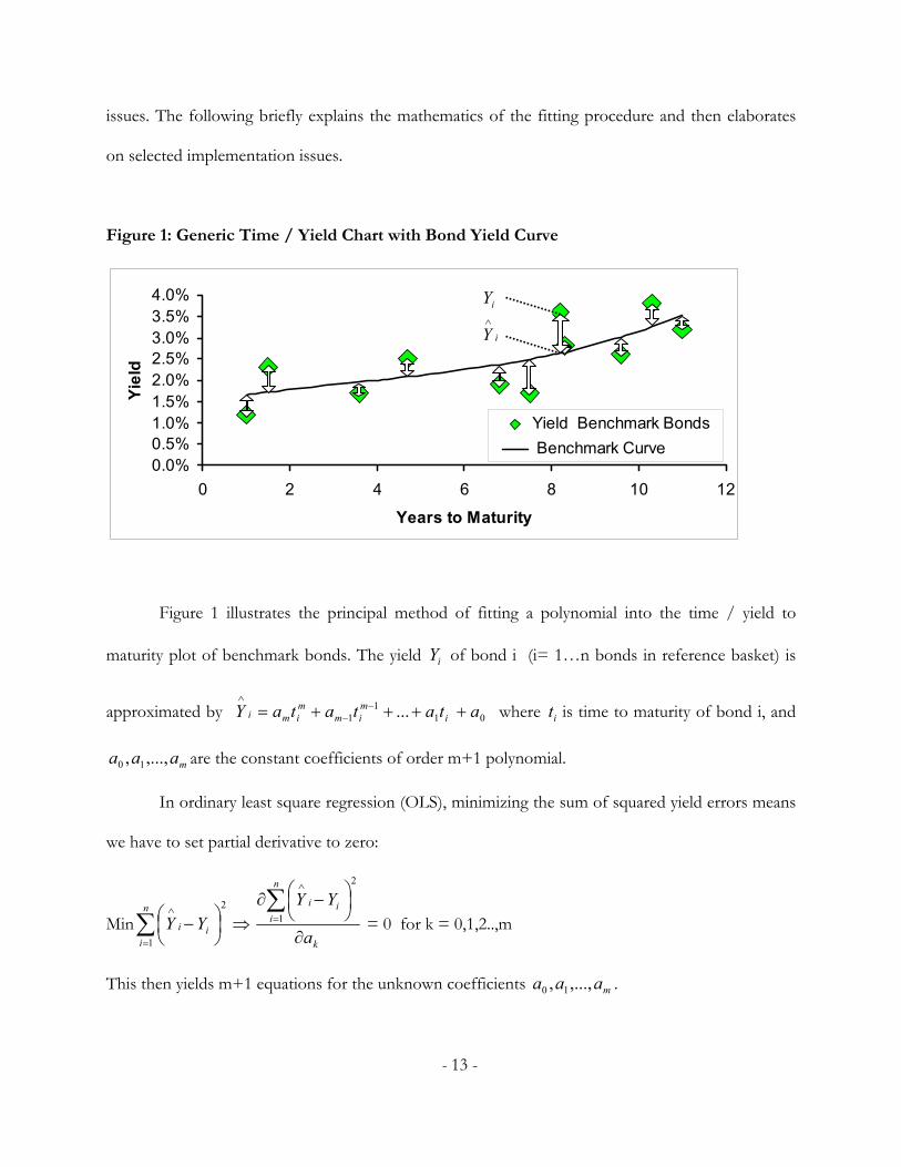
issues. The following briefly explains the mathematics of the fitting procedure and then elaborates
on selected implementation issues.
Figure 1: Generic Time / Yield Chart with Bond Yield Curve
0.0%0.5%1.0%1.5%2.0%2.5%3.0%3.5%4.0%
0 2 4 6 8 10 12
Years to Maturity
Yiel
d
Yield Benchmark Bonds Benchmark Curve
Figure 1 illustrates the principal method of fitting a polynomial into the time / yield to
maturity plot of benchmark bonds. The yield iY of bond i (i= 1…n bonds in reference basket) is
approximated by 011
1 ... atatataY imim
mimi ++++= −
−
∧
where it is time to maturity of bond i, and
maaa ,...,, 10 are the constant coefficients of order m+1 polynomial.
In ordinary least square regression (OLS), minimizing the sum of squared yield errors means
we have to set partial derivative to zero:
Min ⇒
−∑
=
∧n
iii YY
1
2
k
n
iii
a
YY
∂
−∂∑
=
∧
1
2
= 0 for k = 0,1,2..,m
This then yields m+1 equations for the unknown coefficients maaa ,...,, 10 .
i
i
Y
Y∧

- 14 -
Some algebra shows that maaa ,...,, 10 must be a solution of the following system of linear
equations using matrix notation:
=
×
∑
∑∑∑
∑∑∑∑
∑∑∑∑∑∑∑∑∑∑∑
++
+
+
n
mii
nii
nii
ni
m
n
mi
n
mi
n
mi
n
mi
n
mi
ni
ni
ni
n
mi
ni
ni
ni
n
mi
ni
ni
tY
tY
tY
Y
a
aaa
tttt
tttt
tttt
tttn
::
::
....:..:::.:::
...
....
....
22
1
0
221
2432
132
2
In the illustration model, this system is solved numerically by the well known LU
decomposition algorithm as described in Press et al. (1992, p. 43). As coefficients like
∑n
mit2 become an extremely large number for higher dimensions of m, the algorithm will lose
accuracy. However, this is not an issue in general because meaningful interpolations will not exceed
3rd to 4th order polynomials.
Once the approximated yields ∧
iY have been calculated, one can then determine the
corresponding model prices ∧
iP using an market convention yield formula (e.g. RBNZ, 1997, p. 12).
As the model will derive benchmark polynomials for each the bid and ask yield, there will be both a
bid and ask model prices. A buy (sell) signal is generated, if the bid (ask) price in the market exceeds
(is below) the ask (bid) model price found by the model. There is a feature to decrease the sensitivity
of the model by introducing a filter rule so recommendations are only generated if these prices are a
set absolute amount apart. These simple rules for generating recommendations are illustrated in
Figure 2.

- 15 -
Figure 2: Buy /Sell Signal Rules Simple Yield to Maturity Benchmarking Model
FairPriced
Signal BUY - - - - - - SELL
UNDERPRICED OVERPRICED
Sensitivity
Sensitivity
Market price ask
bid
ask
bid ask
bid
ask
bid
ask
bid
ask
bid ∧
iP
∧
iP∧
iP
∧
iP
∧
iP
iP
Another reality of operational models is that some data might suddenly be missing and this
has to be handled. In the solution presented here, missing data are replaced by last known historical
(e.g previous day) prices. It makes sense to suppress corresponding buy/sell signals in these
instances.
The model is also set up to handle callable bonds in a simplified way. For each bond, it
determines the so-called yield to worst which is the lower of either bond to maturity or the yield to
the next call. If the call yield is lower, the bond’s maturity will be set to the next call date for
benchmarking purposes. It does thus not employ more advanced call feature analytics such as the
often used option adjusted spread analysis12.
12 This methodology is described in Windas (1993) of Bloomberg based on the Black,
Derman, & Toy (1990) interest model. Under this approach, a callable bond is viewed as a long
position of an option-free bond plus a short call on the bond (sold to the issuer).

- 16 -
To mention a final feature, the model contains some utility macros for illustrative purposes.
For operational use, it does not suffice to simply link the model to real time trading prices. The
basket will be subject to continuous change and so one needs utilities to deal with additions to and
deletions from the reference basket. Such macros would be data source specific but the scripts
shown in the implementation give a flavor of what would have to be automated.
2.2.2 JP Morgan Discount Factor Model (JPM)
The JPM model illustrates how to overcome the weakness pure yield to maturity based
analysis. The model is, respectively was known in the market as the JP Morgan discount factor
model (JPM) but original documentation could not be uncovered for the purposes of this article. A
review of the literature revealed that this model is in actual fact a simple version of the McCulloch
(1971; 1975) spline approach without node points (as discussed in Anderson et al., 1996, p.25). In
line with McCulloch, the model works with the discount function which means the minimizing
function can be found using least squares as illustrated below. An advantage of refraining from
modeling the spot rate curve is that the discount curve “much better behaved” to use a colloquial
terms. This function has a clear boundary at time zero and is monotonicly declining over time.
The implementation of this spline model is stored in the file named “Term structure JP
Morgan Model (Feb04).xls”. It is more generalized than the earlier yield to maturity model in that it
just fits one benchmark to the mid price which is calculated as the mean of bid and ask price.
Accordingly, there is no selection of bonds as shown in figure 2 but simply a calculation of the
residuals. Similarly, no examples of utilities are included. The following explains the mathematics of
the discount factor fitting in this case and then the main model parameters on a screen shot.

- 17 -
In line with present value pricing function (1) the bonds in the reference basket with market
prices P = [p1,p2, … , pn]T should all be equal to the present value of future cash flows:
( )( )
( ) ntntntntn
tttt
ttt
p
pp
dcdcdcdc
dcdcdcdcdcdcdc
nnjnnn=
==
++++++
+++++++
:1...
:.........
:::1
1
2
1
2222
111
,,2,1,
4,23,22,21,2
3,12,11,1
where ci is the fixed coupon rate of bond i = 1…n; jit
d,
is the discount factor at jit , , which
is the time of the jth coupon of bond i.
The approximation of jit
d,
is chosen as the polynomial 0,11
,1, ... atatata jim
jimm
jim ++++ −− .
To simplify, the further solution is developed just for the three dimensional case of a cubic
spline. Note, however, that the model implementation can cope with higher order polynomials.
Rewriting above equations for m=3 in matrix notation, one finds:
=
×
∑∑∑
∑∑∑∑∑∑∑∑∑
n
jjnn
jjnn
jjnnn
jj
jj
jj
jj
jj
jj
jj
jj
jj
p
ppp
aaaa
tctctcc
tctctcc
tctctcc
tctctcc
:::::
3
2
1
3
2
1
0
3,
2,,
3,33
2,33,333
3,22
2,22,222
3,11
2,11,111
We are thus looking for the vector of coefficients [ ]TaaaaA 3210 ,,,= that minimizes the sum
of the squared difference between the market price vector [ ]TnpppP ..., 21= and model price vector
T
npppP
=
∧∧∧∧
..., 21 , i.e. Min ∑=
∧
−
n
iiPP i
1
2

- 18 -
Setting the partial derivatives to zero: k
n
iii
a
pp
∂
−∂∑
=
∧
1
2
= 0 for k = 0,1,2,3
… , yields four equations for the four unknown 3210 ,,, aaaa .
Defining C=
=
∑∑∑
∑∑∑∑∑∑
jjnn
jjnn
jjnnn
jj
jj
jj
jj
jj
jj
nnnn tctctcc
tctctcc
tctctcc
CCCC
CCCCCCCC
3,
2,,
3,22
2,22,222
3,11
2,11,111
4,3,2,1,
4,23,22,21,2
4,13,12,11,1
::::::::,
…, one must thus solve the system of following system of linear equations to find the coefficient
vector A::
( ) ( )PCCCAPCACC TTTT ××=⇒×=×−1
The model prices are then found by multiplying matrix C with the coefficient vector A:
∧
=× PAC
Bonds priced below [above] their corresponding model price are “cheap” [“rich”].
The residual vector of (under pricing)/over pricing [ ]TnrrrR ..., 10= is then:
PACPPR −×=−=∧
2.2.3 Boundary conditions
Typically constraints are introduced to force the discount factor at time zero to one which is
obviously a most reasonable assumption. This means coefficient ao is set to 1. Moreover, one often
chooses the first derivative of the discount function at time zero to fit a short-term rate, e.g.
overnight bank rate observed in the market. For an assumed short-term rate ro, a1 becomes minus
the continuously compounded equivalent of the short rate, respectively in terms of the annual

- 19 -
equivalent rate a1= - rc = - ln(1 + rann) where rann is the short-term rate expressed as an annual
equivalent yield and rc is the short-term rate expressed as an continuously compounded yield.
This result is derived in footnote 13.
Figure 3: JPM model screenshot
Settlement date14-Feb-99
Coupon Maturity Bid Ask Mid JPM Fair Price (cheap) / rich6.50% 15-Feb-00 100.563 100.583 100.57% 101.17% (0.60%) a0 18.00% 15-Feb-01 102.786 102.854 102.82% 104.48% (1.66%) a1 -0.04879016
10.00% 15-Mar-02 108.406 108.526 108.47% 111.34% (2.87%) a2 -0.002228665.50% 15-Apr-03 96.673 96.827 96.75% 97.27% (0.52%) a3 0.0001970768.00% 15-Apr-04 105.034 105.234 105.13% 106.56% (1.43%) a4 #N/A8.00% 15-Nov-06 106.518 106.809 106.66% 106.06% 0.61% a5 #N/A7.00% 15-Jul-09 100.549 100.903 100.73% 98.91% 1.81% a6 #N/A6.00% 15-Nov-11 91.666 92.049 91.86% 92.83% (0.97%) a7 #N/A
Model Parameters
deg 3 Degree JP Morgan polynomialrestr 0.05 0: no restrictions, 1:DF(t=0) =1, other values: short ratefrequency 2 Number of coupon payments per year
JPM Coefficients
Discount Function
0
0.2
0.4
0.6
0.8
1
- 2 4 6 8 10 12
Zero Rates
0.0%1.0%2.0%3.0%4.0%5.0%6.0%7.0%8.0%
- 2 4 6 8 10 12
13 The discount factor at time ( )tt ∆+0 for cr continuously compounded yield with Taylor
expansion of exponential function
( ) ( ) ( ) ...21... 222
020100000 +∆+∆−==+∆++∆++ −−−∆+− tertereettattaa cccc rt
crt
crtrtt

- 20 -
The parameters as well prices are set in yellow shaded areas. The major parameters are …
deg: Allowing a choice of the degree of the discount function polynomial.
It is not meaningful to choose a much larger value for the small bond universe in the
example.
restr: 0 means no restrictions on discount function, 1 means discount function is forced to
one for t=0 which means coefficient ao is set to one. Any other value is assumed to be
the short-term rate (annual effective yield, i.e. non-continuous yield). a1 is calculated
with the formula given before (ao is forced to one).
frequency: to set number of coupon payments per year.
for 00 =t , 10 =a and omitting second and higher order terms of t∆
( )annccc rratrtrtata +−=−=⇒+∆+∆−=+∆+∆+ 1ln...211...1 1
2221

- 21 -
2.2.4 Extended Nelson & Siegel Model
Nelson and Siegel (1987) proposed a parsimonious model of yield curves that are continuous
and smooth. Unlike the spline models like JPM, Nelson and Siegel (N&S) model the forward or spot
interest rate directly without modeling the discount function first. The model presented here is
structurally similar to the JPM model just shown in that it relies on the same pricing function and
also uses the same small data sample of New Zealand government bonds. It does however not
employ its own estimation procedure, using Solver, Excel’s built-in multidimensional optimization
tool instead. The model is stored in file “NelsonSiegelYieldCurveModel.xls”
The following first explains the yield curve fitting according to the extended N&S model as
described in Bliss (1997) and then talks about particular implementation issues.
Under the extended N&S model, the spot rates r as a function of time m are approximated
by this exponential function:
( )
( )( )21210
2,
,
2
2
1
10,
,,,,,0~
11, 221
ττβββ
σε
ετ
βτ
ββτ
ττ
=Θ
+
−
−+
−
+=Θ
−
−
−
Nwith
eme
memr
jt
jt
mm
jt
m
There are five parameters in parameter vector Θ which can be interpreted as
follows. 0β represents the long-run level of interest rates as ∞→m and for very short times, r will
converge to 10 ββ + . 2β could be interpreted as the medium term component as it will tend to zero
both at the short and long end of the time scale. Finally, the two decay parameters 1τ and 2τ
determine how quickly the effect of the short-term, respectively the medium-term component will

- 22 -
Total
Comp 2
Comp 1
Comp 30.0%
2.0%
4.0%
6.0%
8.0%
10.0%
0 2 4 6 8 10 12
tend to zero. 1τ and 2τ should both be positive to ensure convergence. In the basic version of N&S
(1987) they are set to equal values. Figure 4 visualizes the effect of these three components.
Figure 4: Nelson & Siegel (1987) Spot Rate Components
Contributions of the three N&S
equation terms to the total spot rate
r.
Example parameter values:
0β =5%, 1β =2%, 2β =8%
1τ = 1, 2τ = 1.2
The parameter vector Θ must now be chosen to minimize the sum of squared price errors
ii PP −ˆ , i.e. ( )
∑=
N
iiiw
1
2min ε where ∑ =
= N
j j
ii
D
Dw
11
1and iii PP −= ˆε
Note that in this case the squared errors are actually weighted with the inverse of the bond’s
Macauly duration iD . This means the prices of short-term bonds are fitted much tighter to account
for a greater variability of short-term bond yields.
The estimation procedure needs to be constrained to ensure rate r remain positive and the
implied discount function non-increasing (non-negative forward rates):
( )min0 mr≤ and ( )∞=≤ mr0
where minm is a small value just slightly higher than zero.
(Note that the N&S function is not defined for t=0.)
( )( ) ( )( ) max11expexp mmmmrmmr kkkkk <∀−≥− ++

- 23 -
Finally, similarly to the JPM model, it is often meaningful to prescribe not just positive a sort
term interest rate, i.e. an overnight lending rate, to fix the curve at the short end. This is tantamount
to prescribing a constraint for the sum of 0β and 1β : =+ 10 ββ ( )minmr .
Figure 5: Screenshot of Nelson & Siegel (1987) Bond Relative Value Model
Fitting Extended Nelson & Siegel Spot Rate with Solver programmed by Kurt Hess May 2004, [email protected] to maturity m 3.0 30
Long-run levels of interest rates β0 8.31% 83.09249
Short-run component β1 -3.81% 61.90751
Medium-term component β2 6.41% 64.05964 determines magnitude and the direction of the hump
Decay parameter 1 τ1 9.284 928.3684 determines decay of short-term component, must be > 0
Decay parameter 2 τ2 0.855 85.45838 determines decay of medium -term component, must be > 0
Spot rate at time t rt,i 6.6331%
Objective Functions see formulasNon-weighted objective function x103 0.846957 Inverse duration weighted function x 105 0.135102
Initial Guess Values:
Bond DataShort-term rate 4.50%Settlement date 14-Feb-99
Issuer Coupon Maturity Bid Ask Mid Clean Mid DirtyModel Price Duration Weights (wi) (cheap) / rich
NZ Government 6.50% 15-Feb-00 100.563 100.583 100.57% 103.80% 103.151% 0.956271 0.361346082 0.65%NZ Government 8.00% 15-Feb-01 102.786 102.854 102.82% 106.05% 106.117% 1.821322 0.189721979 (0.07%)NZ Government 10.00% 15-Mar-02 108.406 108.526 108.47% 111.70% 113.102% 2.647526 0.130516077 (1.40%)NZ Government 5.50% 15-Apr-03 96.673 96.827 96.75% 99.98% 97.814% 3.706899 0.093216656 2.17%NZ Government 8.00% 15-Apr-04 105.034 105.234 105.13% 108.37% 108.876% 4.253648 0.081234908 (0.51%)NZ Government 8.00% 15-Nov-06 106.518 106.809 106.66% 109.90% 110.671% 5.884208 0.058724089 (0.78%)NZ Government 7.00% 15-Jul-09 100.549 100.903 100.73% 103.96% 103.283% 7.537708 0.045842151 0.68%NZ Government 6.00% 15-Nov-11 91.666 92.049 91.86% 95.09% 95.317% 8.770603 0.039398058 (0.23%)
6.63%
0.0%
2.0%
4.0%
6.0%
8.0%
10.0%
0 2 4 6 8 10
N&S Zero Rate
Minimize
Minimize
Default Values Set Random Values
Before using the minimization macros, you must establish a reference to the Solver add-in. With a Visual Basic module active, click References on the Tools menu, and then select the Solver.xla check box under Available References. If Solver.xla doesn't appear under Available References, click Browse and open Solver.xla in the \Office\Library subfolder.
Step through optimization
Figure 5 provides a screenshot of the N&S model implementation. There are some
prerequisites for the Excel setup in order to use the Solver software that minimizes the objective
function. One should not be confused by the markedly different shape of the zero yield curve
compared to the curve found through JPM for the same sample universe of New Zealand
government bonds. Fitting a model with five parameters to a purely illustrative basket of only eight
bonds is bound to lead to over fitting problems. Accordingly, the buy/sell signals generated will be
very different.

- 24 -
3 A Heuristic Fitting Method for the Term Structure of Credit Spread
With this section we tackle the second major topic in this paper. There is also the need for
suitable bond relative valuation when credit risk, the second major bond pricing factor, becomes an
important determinant of market price. This section will first expand on the discussion in the
introduction on the nature and dynamics of credit spreads, elaborating first on aspects that affect
credit spreads beyond factors generally assumed in standard academic models. This is followed by a
review of the shape of the term structure of credit spreads, both predicted and observed in the
market. Purpose of this discussion is to provide the rationale and motivation for a heuristic term
structure of fitting method of detecting mispriced which is presented in the final subsection.
3.1 The nature of credit spreads
The credit spread is the most popular yardstick for practitioners to assess bonds subject to
default risk. Measured in basis points, it is typically just derived from redemption yield differentials
to a reference benchmark, e.g. a government bond curve. Once they have done so, they must make a
judgment whether this yield premium compensates them adequately for the risk they assume. This in
turn is much harder and they do not get much help from academic research where there is a healthy
debate on how to explain credit spreads observed in the market in the first place. We mentioned
articles of Fons (1994) and Elton et al. (2001) in the introduction who pointed out that pure default
risk cannot possibly account for absolute yield spreads alone.
Whatever the components of the credit spread, practitioners are more concerned about the
relative pricing of the bonds compared to instruments of equivalent credit quality. Quite naturally,
they turn to credit curves for the same credit rating category but this is by no means the only

- 25 -
decision criteria. Research of Collin-Dufresne et al. (2001) drew attention to the fact that only about
a quarter of spread changes can actually be attributed to factors one would theoretically expect to
influence them. Failing the identify the true driver of spread changes, they coin the expression “local
supply/demand shock” that are independent of both changes in credit risk and typical measures of
liquidity14. One can easily generalize these findings of Collin-Dufresne and state that not just the
changes but also the absolute level of credit spreads are determined by other factors beyond the risk
as assessed by official credit ratings. Academic research has focused on taxation and liquidity aspects
in this respect, probably because these do lend themselves easily to standard empirical analysis15.
While it would be beyond the scope of this paper to tackle this issue here, it is the professional work
experience of this author that credit spreads in a particular case are difficult to understand, in many
instances even lack immediate rational explanation. Here are some examples.
• Household names
So-called “household names” trade on much narrower spreads than indicated by their credit
ratings. An extreme example was Porsche’s unrated 10-year bond issued in April 1997 which
14 While Collin-Dufresne et al. (2001) confirmed that factors important for example in
Black-Scholes (1973) and Merton (1974) contingent claims framework such as a firm’s leverage,
equity returns and volatility indeed had a significant correlation to spread changes, non-firm specific
attributes like the return of the whole share market were a much stronger driving force. Overall their
principal component analysis reveals that there is a large systematic component that lies outside the
model framework.
15 e.g. Van Landschoot (2003) for the Euro corporate bond market

- 26 -
has often traded below the German government curve. A research hypothesis could posit
that such anomalies will occur more frequently in markets with strong retail demand.
• Some spread levels may also be rooted in informational inefficiencies.
These are highlighted in Schultz (2001, p. 678) for the US corporate bond market where the
potential buyer cannot observe all quotes in a central location. Similarly, if a bond of the
same firm trades in different markets, one often observes differences which cannot possibly
be explained by currency, taxation or other factors.
• Spreads are affected by new issue supply
A lead bank may be pressured to “move a transaction off their books” thus affecting
secondary market spreads. Conversely, strong demand for a new issue will tighten spreads of
existing deals.
• Rating assessment of market diverges from official agency ratings.
Official ratings are often not accepted by the gross of market participants who, colloquially
speaking, consider agencies as “behind the curve”. Such cases have for instance been
observed during the 1997 Asian crisis, but agencies also tend to be slow to recognize
improvements in credit quality. Due to the formal internal processes involved, agencies
frequently find it hard to react promptly. It has also been noted that conflicts of interest and
the quasi-monopoly of some agencies may create rating distortions16. All in all, an official
credit rating constitutes just a mostly qualitative assessment of a well informed but not
16 Such concerns are for instance reflected in a SEC concept release SEC (2003) for the
oversight of credit rating agencies.

- 27 -
infallible party.
All these pricing aspects highlight that the particular decision of assessing a relative value of
a bond involves a qualitative, respectively “market savvy” component not easily captured by any of
the standard academic models.
3.2 The shape of the term structure of credit spreads
We have mentioned in the previous section that practitioners will turn to credit curves of
comparable credit quality as a starting point for their relative value valuation. In this section, we
review what is generally predicted and observed regarding the shape of this term structure of credit
spreads.
Figure 6:
Term Structure of Interest Risky Discount Bonds in the Longstaff & Schwartz (1995) Model
Term Structure of Interest Risky Discount Bonds
0%
2%
4%
6%
8%
10%
12%
14%
0 2 4 6 8 10 12Time to maturity
Risky DiscountBond
Moderate RiskDiscount Bond
r at t=0
Yield riskfree bond

- 28 -
Figure 6 illustrates in generic ways the term structure of spot rates of a risky, respectively less
risky discount bond as predicted by many of the mainstream credit risk models. In this instance, it
was generated by the Longstaff & Schwartz (1995) model (L&S 95) which, for illustration, is
explained in more detail in Appendix 2. L&S 95 is from the family of Merton’s (1974) contingent
claims models but one would find similar hump-shaped, downward-sloping credit yield curves for
example in Jarrow, Lando & Turnbull’s (1997) reduced form approach.
This theoretical prediction appears to be backed by empirical studies such as Fons (1994, p.
30) who estimates a cross-sectional regression of spreads on maturity and finds significantly negative
coefficients for single B bonds. This result is also supported by Moody’s default data where marginal
default rates of speculative grade bonds (B rating) exhibit a declining trend with longer time
horizons.
The intuition behind this result is that speculative firms, being very risky at issuance, have
room to improve, i.e. the longer the time to maturity, the more likely the value of the firm will rise
substantially. Another interpretation would be that speculative bonds obtain the character of an
equity instrument and are thus traded on a break-up value instead of a yield basis. Conversely, high
grade credit “can only become worse” through time and thus show an upward sloping term
structure of credit spread.
These results are somewhat against the intuition of practitioners who observe that where a
firm issues in two separate time tranches, it will be asked offer a higher yield premium for the longer
maturity tranche of the transaction and this applies equally to weaker and stronger credits. Helwege
& Turner (1999) indeed provide some empirical evidence for this observation. They argue that
downward sloping credit curves are a result of “safer” speculative grade firms issuing longer-dated
bonds which in turn leads to a sample selection bias.

- 29 -
What we can conclude is that there are two schools of thought for modeling term structure
of credit spreads. A useful bond relative value tool for corporate bonds must thus be capable of
accommodating both of them.
3.3 Heuristic fitting method for term structure of credit spreads
This section presents an approach for work tool so market practitioners can firstly, assess
the relative price of a bond in view of less tangible pricing factors (as shown in section 3.1) and
secondly, to prescribe a term structure of credit spreads they feel is appropriate for the particular
instrument and market condition (as explained in section 3.2). The implementation of this model is
shown in file “Cheap Rich List (Feb04).xls”. The file uses a sample of Swiss corporate industrial
bonds to generate a list of cheap, respectively rich bonds. It employs a simple redemption yield
based reference curve of the type that was derived in section 2.2.1 as a basis to calculate credit
spreads. This yield to maturity based approach could easily be adapted into a spot rate framework
using curve derived in section 2.2.2 or 2.2.3. Yet given the heuristic nature of the model, this is likely
to add only limited value. The following describes the model with a simplified numerical example
also documented in the Excel work book.
3.3.1 Defining the term structure of credit spreads in the model
The model lets the user choose the desired term structure of credit spreads for each rating
category by means of shape parameters. This is illustrated through a numerical example in Figure 7
below. The term structure is basically broken down into two sub-periods. A short- to medium term
period to T∞ (T_indef) which is followed by the long-term characteristics of the credit spread.

- 30 -
Figure 7: Explanation Shape Parameters Term Structure of Credit Spreads
300bps/yr (Slope at t=0)
T_indef=3
S_indef=125
6.125
Spread Lower Limit (70.0% of 125bps)
-12 bps/yr (Slope at t=T_indef)
0
50
100
150
200
250
0 1 2 3 4 5 6 7 8Years to Maturity
Cre
dit S
prea
d
Term Structure for a4 = 3
Term Structure for a4 = -3
As to the first period, a fifth order polynomial is fitted between zero and T∞.
( ) 44
33
2210 tatatataatSpread ++++=
It must meet the following three boundary conditions:
• must be zero a time = 0 which means 00 =a
• must reach S∞(S_indef) at time t=T∞.
• slope at point S∞/T∞ must equal the slope of the long-term curve beyond T∞. (more details
on this slope are below)
The user affects the shape of the polynomial with two parameters.
• The initial slope (in bps per year) at time = zero may be specified
• The shape of the hump is also affected by parameter a4 which corresponds to the fifth
order coefficient of the polynomial. Figure 3 shows the term structure for a4= 3,
respectively minus 3.
Short-term characteristics of credit spreads
Long-term characteristics
T
- 31 -
In the long-term horizon, the user can specify a slope for the further development of credit
spreads. In most cases it will be set to or slightly above zero to obtain constant or moderately
increasing credit spreads beyond time T∞. There is also the option to specify a lower limit below
which the credit spread may never decline. This parameter is set as a percentage of S∞. If this lower
limit is specified as a number greater than one, it actually becomes an upper limit specification.
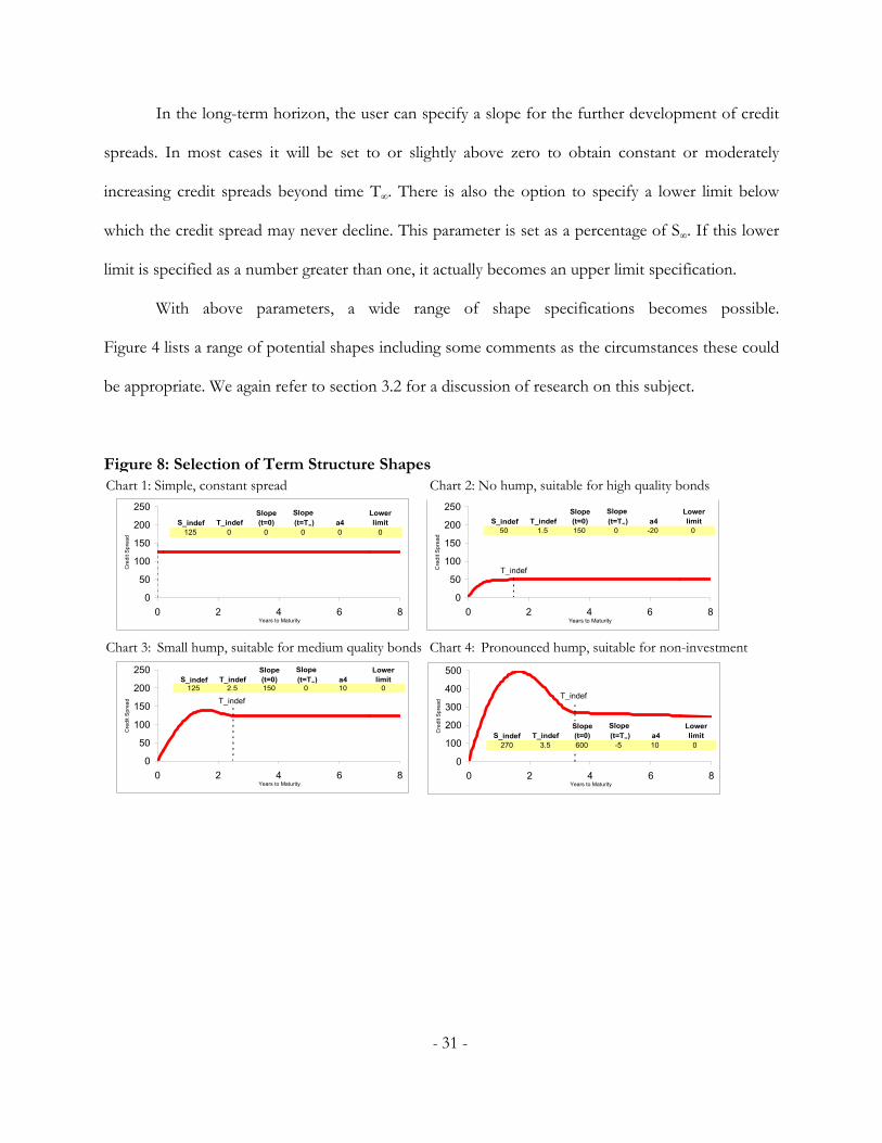
With above parameters, a wide range of shape specifications becomes possible.
Figure 4 lists a range of potential shapes including some comments as the circumstances these could
be appropriate. We again refer to section 3.2 for a discussion of research on this subject.
Figure 8: Selection of Term Structure Shapes
0
50
100
150
200
250
0 2 4 6 8Years to Maturity
Cre
dit S
prea
d
T_indef
0
50
100
150
200
250
0 2 4 6 8Years to Maturity
Cre
dit S
prea
d
T_indef
0
50
100
150
200
250
0 2 4 6 8Years to Maturity
Cre
dit S
prea
d T_indef
0
100
200
300
400
500
0 2 4 6 8Years to Maturity
Cre
dit S
prea
d
S_indef T_indefSlope(t=0)
Slope (t=T∞) a4
Lowerlimit
125 0 0 0 0 0S_indef T_indef
Slope(t=0)
Slope (t=T∞) a4
Lowerlimit
S_indef T_indefSlope(t=0)
Slope (t=T∞) a4
Lowerlimit
S_indef T_indefSlope(t=0)
Slope (t=T∞) a4
Lowerlimit
50 1.5 150 0 -20 0
125 2.5 150 0 10 0
270 3.5 600 -5 10 0
Chart 1: Simple, constant spread Chart 2: No hump, suitable for high quality bonds
Chart 3: Small hump, suitable for medium quality bonds Chart 4: Pronounced hump, suitable for non-investment

- 32 -
3.3.2 Detecting cheap/rich bond with heterogeneous credit quality:
a simplified numerical example
For illustration, the following tables (Table 2 and 3) and figures (Figure 9) present a
simplified numerical example of cheap/rich analysis. There are three bonds analyzed. Bond I has an
AA rating while bonds IIa and IIb are rated BBB. A buy [sell] signal is generated if the model price
based on the target spread is above [below] the market price.
Table 2: Data Example Bonds
Bond I IIa IIb
Rating AA BBB BBB
Price ($ per $face value)* 102 99 106
Coupon (paid once annually) 4.00% 4.00% 4.00%
Time to Maturity 2.79 yrs 5.20 yrs 7.79 yrs
Yield to Maturity 3.24% 4.22% 3.12%
Spread to Benchmark 136 bps 208 bps 58 bps
Target Spread (derived from
parameters in Table 3) 50 bps 122 bps 120 bps
Model Yield 2.37% 3.36% 3.73%
Model Price (MP) * 104.338 103.016 101.761
MP > Price MP > Price MP < Price
Recommendation Cheap Bond:
Buy
Cheap Bond:
Buy
Rich Bond:
Sell
* Price excluding accrued interest

- 33 -
Figure 9: Generic Yield to Maturity Based Cheap Rich Analysis
2.37%3.36% 3.73%3.24%4.22%
3.12%
1.0%2.0%3.0%4.0%5.0%
0 2 4 6 8 10Years to Maturity
Yield
Yield examplebonds
Model yieldaccording totarget spread
Benchmark curve(polynomialdegree 3)
102.0
99.0
106.0104.34
103.02101.76
95
100
105
110
0 2 4 6 8 10Years to Maturity
Bond
Pric
e
Prices examplebonds
Model pricesaccording to targetspread
-50
100150
0 2 4 6 8 10Years to Maturity
Targ
et S
prea
d( i
n bp
s)
Bond IIa&b,Rating BBB
Bond I, RatingAA
Buy Buy Sell
Table 3: Term Structure of Credit Spread Shape Parameters
Rating AA BBB
S∞ (in bps) 50 125
T∞ 1 2.5
Slope (t=0) 200 200
Slope (t=T∞) 0 -1
“Hump parameter” a4 -6 2
Lower limit (as % of S∞) 0.8 0.8

- 34 -
Compared to the main model, the version above is simplified in these aspects. The
illustrative example does not take bid/ask spreads into consideration when generating buy/sell
signals. To limit the number of recommendations the user may specify a sensitivity parameter to
suppress recommendations where the price is very close to the model price. The sensitivity chosen
could, for instance, take transaction charges into account. This the same filter described in Figure 2
for the model in section 2.2.1. For shorter bonds typical price changes in less liquid markets may
lead to very erratic yield moves that do translate into meaningful buy/sell signals. The user may thus
exclude the analysis for very short-term bonds. Finally, the main model provides statistics on the
credit spreads observed in the reference baskets. An example is shown in Figure 10 below.
Figure 10: Generic Yield to Maturity Based Cheap Rich Analysis
Analysis credit spreads Swiss industrial bonds 26/02/1999 0:00
Internal Rating AAA AA A BBB BB B Other Grand TotalNumber of bonds 1 9 36 31 10 1 10 98Average spread to Swiss Govt (bps) 4 63 71 125 252 265 74 108Min of spread (bps) 4 8 20 51 44 265 23 4Max of spread (bps) 4 175 189 259 915 265 127 915Years to maturity/ next call (average) 1.8 5.0 4.2 4.5 3.9 6.3 5.9 4.5
Average Credit Spread by Internal Rating
050
100150200250300350400450500
Average 4 63 71 125 252 265 74 108
AAA AA A BBB BB B Other Grand Total

- 35 -
3.3.3 Some remarks on how to apply the model
The model description has not addressed the issue of calibration yet. In other words, how
should one determine the shape parameters for a particular instrument, respectively group of
instruments? Given that this is not a fitting method for empirical research purposes, the following
pragmatic method is recommended.
In a first instance, one would select a value for S∞. If we leave all other parameters zero, this
is nothing else than a flat credit spread we apply to a reference curve, i.e. parallel upward shift of the
reference curve. For many users this is the ad-hoc method they will be used to and, reflecting on the
empirical results of Fons (1994) discussed earlier17, this is not an unreasonable approach at all. To
automate the selection of S∞, one could derive it from a mean value for rating category as shown in
the analysis Figure 10. Note that the rating category of a particular bond may be set by the user and
would not necessarily coincide with an official agency rating.
With regard to the remaining shape parameters, it is not meaningful to set them for just one
rating class. One would select, for example, common values for all BBB- to BBB+ rated bonds. As
per section 3.2, there will be no hump for most rating categories and we would simply set a value for
T∞ in the range of 1- 2 years, some generic slope at time t=0 (in bps per year) and a4 to zero. The
parameter of concern would be the slope at time t= T∞. This could be determined by a Fons (1994,
p. 30) type regression analysis although it does most probably not make sense to update it as
regularly as the main spread parameter S∞.
17 Fons (1994) finds rather flat slopes for most rating categories and although t-statistics
indicates values significantly different from zero, R2 values are quite low.

- 36 -
Finally, in respect to speculative grade rating categories, there is obviously the option to set
prescribe a hump-shaped structure unless the user prefers increasing term structure in line with
Helwege & Turner (1999). In most bond market supply of these segment is rather sparse and a
ballpark prescription of parameters without actual calibration of values may well be appropriate.

- 37 -
4 Conclusion
This paper illustrated the implementation of some models for yield curve fitting used in
trading applications, something not yet formally documented in the academic literature. For bonds
subject to credit risk it presented a heuristic model to obtain information on over-, respectively
underpriced bonds. Both types of model implementations document the pragmatic nature of such
solutions. In the absence of conclusive results by academic researchers, these models generate buy
and sell signals as a result of the main pricing parameter for fixed income instruments which are
interest rates, respectively credit spreads. The user can then evaluate them in view of his/her
knowledge of local supply and demand aspects and other qualitative factors such as the ones listed
in section 3.1.
There is another more general lesson one could learn from these models, which in terms of
complexity are much simpler than most of the approaches currently advocated in quantitative
literature. Even though their approach is static without the ambition of justifying them in a dynamic
or non-arbitrage consistent theoretical framework, they “can be handled and understood” by the
practitioners. More advanced approaches usually start from an idealistic premise about how the
world should look like, respectively how rational investors should act. Researchers then find that
realty is different and attempt to save the approach with progressively more sophisticated
amendments and extensions. This could almost be compared to a “mathematical arms race” where
increasingly complex quantitative theories are applied without markedly improving the predictive
power of the models. Interest rate modeling is a good example where only models calibrated
continuously to current market rates do have any meaningful applications in the market. It would
perhaps be time that academic research in finance made the requirements of market practitioners a

- 38 -
starting point for improved models and not a futile chase for the ultimate true model that does not
exist.

- 39 -
5 References
Anderson, N., Breedon, F., Deacon, M., Derry, A., & Murphy, G. (1996). Estimating and interpreting the yield curve. Chichester: John Wiley Series in Financial Economics and Quantitative Analysis.
Black, F., Derman, E., & Toy, W. (1990). A One-Factor Model of Interest Rates and Its Application to Treasury Bond Options. Financial Analysts Journal, 46(1), 33-38.
Black, F., & Scholes, M. (1973). The pricing of options and corporate liabilities, Journal of Political Economy (Vol. May - June 1973, pp. 637-654).
Bliss, R. R. (1997). Testing Term Structure Estimation Methods. Advances in Futures and Options Research(9), 197-231.
Christie, D. (2003). Accrued Interest & Yield Calculations and Determination of Holiday Calendars Version 2.2. Swiss Exchange. Retrieved, from the World Wide Web: http://www.swx.com/products/aic_202_en.pdf
Collin-Dufresne, P., Goldstein, R., & Martin, J. S. (2001). The Determinants of Credit Spreads Changes. Journal of Finance, 56(6), 2177-2207.
Cox, J. C., Ingersoll, J. E., Jr., & Ross, S. A. (1985). An Intertemporal General Equilibrium Model of Asset Prices. Econometrica, 53(2), p. 363-384.
Duffie, D., & Lando, D. (2001). Term structures of credit spreads with incomplete accounting information. Econometrica, 69(3), 633-664.
Elton, E. J., Gruber, M. J., Agrawal, D., & Mann, C. (2001). Explaining the Rate Spread on Corporate Bonds. Journal of Finance, 56(1), 247-277.
Fabozzi, F. J. (1999). Bond Markets, Analysis and Strategies (4th ed.). Englewood Cliffs, N.J., USA: Prentice Hall.
Fisher, M., Nychka, D., & Zervos, D. (1995). Fitting the term structure of interest rates with smoothing splines, Finance and Economics Discussion Series 1: Federal Reserve Board.
Fons, J. S. (1994). Using default rates to model the term structure of credit risk, Financial Analysts Journal (Vol. 50, pp. 25-32). Charlottesville.
Heath, D., Jarrow, R., & Morton, A. (1992). Bond Pricing and the Term Structure of Interest Rates; A New Methodology. Econometrica, 60(1), 77-105.
Helwege, J., & Turner, C. M. (1999). The slope of the credit yield curve for speculative-grade issuers. Journal of Finance, 54(5), 1869-1884.
Ho, T. S., & Lee, S. B. (1986). Term Structure Movements and Pricing Interest Rate Contingent Claims. Journal of Finance, 41, 1001-1029.

- 40 -
Houweling, P., Hoek, J., & Kleibergen, F. (2001). The joint estimation of term structures and credit spreads. Journal of Empirical Finance, 8, 297–323.
Ioannides, M. (2003). A comparison of yield curve estimation techniques using UK data. Journal of Banking & Finance, 27(1), 1-26.
Jarrow, R. A. (1997). A Markov Model for the Term Structure of Credit Risk Spreads. The Review of Financial Studies, 10(2), 481-523.
Krippner, L. (2003). Optimising fixed interest portfolios with an orthonormalised Laguerre polynomial model of the yield curve.Unpublished manuscript, [email protected].
Longstaff, F. A., & Schwartz, E. F. (1995). A Simple Approach to Valuing Risky Fixed and Floating Rate Debt. Journal of Finance, 789-819.
McCulloch, J. H. (1971). Measuring the Term Structure of Interest Rates. Journal of Business, 44, 19-31.
McCulloch, J. H. (1975). The Tax-Adjusted Yield Curve. Journal of Finance, 30, 811-829.
Merrill Lynch. (2004). Rich / Cheap Report: Bond Indices Group, Merrill Lynch Bond Indices & Analytics.
Merton, R. C. (1974). On the pricing of corporate debt: The risk structure of interest rates, Journal of Finance (Vol. 29, pp. 449–470).
Nelson, C. R., & Siegel, A. F. (1987). Parsimonious modeling of yield curves, Journal of Business (Vol. 60(4), pp. 473—489).
Press, W. H., Flannery, B. P., Teukolsky, S. A., & Vetterling, W. T. (1992). Numerical recipes in C: the art of scientific computing: Cambridge University Press.
RBNZ. (1997). Information Memorandum New Zealand Government Bonds. Reserve Bank of New Zealand / The Treasury New Zealand Debt Management Office. Retrieved, from the World Wide Web: http://www.nzdmo.govt.nz/govtbonds/bond-memo-1997.pdf
Rebonato, R. (1998). Interest-rate option models : understanding, analysing and using models for exotic interest-rate options: Wiley, Chichester ; New York.
Reilly, F. K., & Brown, K. C. (1997). Investment Analysis and Portfolio Management (5th ed.): Dryden Press.
Schaefer, S. M. (1977). The Problem with Redemption Yields. Financial Analysts Journal, 33(4), 59-67.
Schultz, P. (2001). Corporate Bond Trading Costs: A Peek Behind the Curtain. Journal of Finance, 56(2).

- 41 -
SEC. (2003). Concept Release: Rating Agencies and the Use of Credit Ratings under the Federal Securities Laws, Release Nos. 33-8236. U.S. Securities and Exchange Commission. Retrieved May 4, 2004, from the World Wide Web: http://www.sec.gov/rules/concept/33-8236.htm
Sercu, P., & Wu, X. (1997). The information content in bond model residuals: An empirical study on the Belgian bond market. Journal of Banking & Finance, 21(5), 685-720.
Svensson, L. (1994). Estimating and interpreting forward interest rates: Sweden 1992-4. Discussion paper, Centre for Economic Policy Research(1051).
Van Landschoot, A. (2003). The Term Structure of Credit Spreads on Euro Corporate Bonds. Working Paper Center for Economic Research, Tilburg University. Retrieved February, 2004, from the World Wide Web: http://greywww.kub.nl:2080/greyfiles/center/2003/doc/46.pdf
Vasicek, O. A. (1977). An Equilibrium Characterization of the term structure, Journal of Financial Economics (Vol. 5, pp. 177-188).
Windas, T. (1993). An Introduction ot Option-Adjusted Spread Analysis. New York: Bloomberg Magazine Publications.

- 42 -
Appendix 1:
Settlement Price Calculation New Zealand Domestic Bond Market
According to the Reserve Bank of New Zealand Formula (RBNZ 1997)
+
+
++
= ∑=
n
n
kk
ba i
FVi
C
iP
)1()1()1(
10
where
P: Market Value of Bond
FV: Nominal or face value of bond
i: Annual market yield / 2 (in %)
c: Annual coupon rate in %
C: Coupon Payment (= c/2 * FV) – semi-annual coupon
n: Number of full coupon periods remaining until maturity
a: Number of days from settlement to next coupon date
b: Number of days from last to next coupon date

- 43 -
Appendix 2:
Longstaff & Schwartz 1995 Model
In their 1995 Journal of Finance paper, Longstaff and Schwartz (L&S 95) show a simple
approach to value risky debt subject to both default and interest rate risk. In line with the traditional
Black-Scholes (1973) and Merton (1974) contingent claims-based framework, default risk is modeled
using option pricing theory. This means default occurs if the level of asset of a firm (V) falls below a
bankruptcy threshold (K). V is assumed the follow the following stochastic process
1VdZVdtdV σµ +=
where σ is the instantaneous standard deviation of the asset process (constant) and 1dZ is a
standard Wiener process.
Similarly, interest rates are assumed to follow a standard Vasicek process (Vasicek 1997) as
follows:
( ) 2dZdtrdr ηβζ +−=
where
ζ is the long-term equilibrium of mean reverting process (constant)
β is the "pull-back" factor - speed of adjustment (constant)
η is the spot rate volatility (constant)
2dZ is a standard Wiener process.
The instantaneous correlation between 1dZ and 2dZ is dtρ
L&S 95 then derive the value of a risky discount bond as

- 44 -
( ) ( )TrXQTrwDTrDTrXP ,,,),(),,( −=
Thus the price of this bond is a function of X, which corresponds to the ratio of V/K, the
interest rate r, and the time to maturity T. The terms to be calculated are explained below.
( ) ))(),( rTBTAeTrD −= is the value of riskfree (no credit risk) discount bond according to Vasicek
(1977) with
( ) ( )1412)( 23
2
23
2
2
2−
−−
−+
−= −− TT eeTTA ββ
βη
βα
βη
βα
βη
α
βTeTB−−
=1)(
Here α represents the sum of the parameter ζ plus a constant representing the market price
of risk, β is defined above
The Q(X,r,T) term can be interpreted as probability - under risk neutral measure - that
default occurs. It is the limit of ),,,( nTrXQ as ∞→n .
),,,( nTrXQ is calculated as follows:
∑=
=n
iiqnTrXQ
1),,,( with
( )
( ) ( ) nibNqaNq
aNqi
jjijii ,.....,3,2,
1
1
11
=−=
=
∑−
=
where N(.) denotes the cumulative standard normal distribution and
( )( )niTS
TniTMXai,ln −−
= ( ) ( )( ) ( )njTSniTS
TniTMTnjTMb ji −−
=,,

- 45 -
Expressions ),( TtM and )(TS are defined as follows:
( ) ( )( )
( )( )
( ) ( )( )tT
tr
tT
tTtM
βββ
η
ββη
βα
β
βββ
ηβ
ρση
σβη
βρσηα
−−−
−
−−
+−+
−−
++
−−
−=
exp1exp2
exp1
1expexp2
2),(
3
2
3
2
2
3
2
2
2
2
2
and ( )( )
( )( )t
t
tTS
ββ
η
ββη
βρση
σβη
βρση
2exp12
exp12
)(
3
2
3
2
2
22
2
−−
+
−−
+−
++=
As a reminder, ρ is the instantaneous correlation between the asset and interest rate
processes.
Finally, the constant parameter w is the write-down in case of a default in percent of the face
value. In other words, it is one minus the recovery rate in case of a default.
Once the value of a pure discount bond is found, the value of a coupon bond is simply
valued as series of discount bonds consisting of coupons and principal repayment. Note that L&S
95 also derive a closed form solution for perpetual floating rate debt in a similar fashion.
The authors conclude their work with an empirical model validation. They conduct a
regression analysis of how historically observed spreads (sourced from Moody’s) have correlated
with the return of share indices as a proxy for the asset process, respectively change in interest rates.
They indeed find significant negative correlations in most cases with both interest rate changes and
development of asset prices. Just for high grade bonds (AAA and AA bond) they determined less
significance for the asset correlation coefficient. This may be expected though because the “well
cushioned” high grade credits will be less affected by downturns in the share market.

- 46 -
As an illustration of the L&S 95 model outputs, the charts belwo show the value and yield of
a discount bond as a function of time to maturity T for the parameters in Table A2.1.
Figure A2.1: Risky discount bond prices as a function of bond tenor (time to maturity)
0%
10%20%
30%
40%50%
60%
70%
80%90%
100%
0 2 4 6 8 10 12Time to maturity
Value risky discount bond(L&S 95) Value risk free discount bond(Vasicek)
Figure A2.2: Term Structure of Interest Risky Discount Bonds
Term Structure of Interest Risky Discount Bonds
0%
2%
4%
6%
8%
10%
12%
14%
16%
0 2 4 6 8 10 12Time to maturity
Risky DiscountBond
r at t=0
Yield riskfree bond

- 47 -
Table A2.1: Parameters L&S 95 Model Example
Parameter description Symbol Value
Rate r0 at t=0 r 7.0%
"Pullback" factor interest rate β 1.00
Instantaneous standard deviation of short rate η 3.162%
η2 0.0010
α in L&S = ζ + constant α 0.060
V0/K =X (measure of initial credit quality) X 1.30
Writedown = 1 - Recovery Rate w 0.50
Volatility of asset value process σ 20.00%
σ2 0.0400
Instantaneous correlation asset/interest rate ρ - 0.25
Iterations for Q n 100