Bonds, Bond Prices, Interest Rates, and the Riskand Term Structure of Interest Rates

ECON 40364: Monetary Theory & Policy

Eric Sims

University of Notre Dame

Fall 2018

1 / 85

Readings

I Text:I Mishkin Ch. 4, Mishkin Ch. 5 pg. 85-100, Mishkin Ch. 6I GLS Ch. 33

I Other:I Poole (2005): “Understanding the Term Structure of Interest

Rates”I Bernanke (2016), “What Tools Does the Fed Have Left? Part

2: Targeting Longer-Term Interest Rates”

2 / 85

BondsI We will generically refer to a “bond” as a debt instrument

where a borrower promises to pay the holder of the bond (thelender) fixed and known payments according to somepre-specified schedule

I Generically, a financial security entitles the holder to periodcash flows

I Hence, bonds are known as fixed income securitiesI There are many different types of bonds. Differ according to:

I Details of how bond is paid offI Time to maturityI Default risk

I The yield to maturity is a measure of the interest rate on thebond, although the interest rate is often not explicitly laidout. Will use terms interest rate and yield interchangeably

I Want to understand how interest rates are determined andhow and why they vary across different characteristics ofbonds

3 / 85

Present ValueI Present discounted value (PDV): something received in the

future is worth less to you than if you received the thing in thepresent

I Discount rate: rate at which you discount future cash flowsfrom a security

I Suppose the discount rate is i and is constantI For a future cash flow (CF ), how many dollars would be

equivalent to you today:

PVt =CFt+n

(1 + i)(1 + i)(1 + i) · · · × (1 + i)

I Here t is the “present,” t + n is the future (n periods away),and i is the discount rate

I The formula reduces to:

PVt =CFt+n

(1 + i)n

4 / 85

Present Value: Example I

I Suppose you are promised $10 in period t + 1

I You could put $1 in bank in period t and earn i = 0.05 ininterest between t and t + 1

I How many dollars would you need in the present to have $10in the future?

(1 + i)PVt = CFt+1

PVt =CFt+1

1 + i

=10

1.05= 9.5238

5 / 85

Present Value: Example II

I Suppose you are promised $10 in period t + 3

I You could put $1 in bank in period t and earn i = 0.05 acrosseach set of adjacent periods between now and then

I If you put $1 in bank in period t and kept it there(re-investing any interest income), you would have(1 + i)(1 + i)(1 + i) dollars in t + 3. Hence, the presentvalue of $10 three periods from now is:

PVt(1 + i)(1 + i)(1 + i) = CFt+3

PVt =CFt+3

(1 + i)3

=10

(1.05)(1.07)(1.03)= 8.6384

6 / 85

Present Value and the Price of an Asset

I A financial asset is something which entitles the holder toperiodic payments (cash flows)

I The classical theory of asset prices is that the price of an assetis equal to the present discounted value of all future cash flows

I The price of a bond (or any asset) is just the presentdiscounted value of cash flows

I The yield is the discount rate you use to discount those futurecash flows

I The yield is also equal to the expected or required return: notnecessarily equal to realized return if security is sold prior tomaturity

I Key issue in asset pricing: how do you determine which yieldto use to discount cash flows and hence price an asset?

I Basic gist: the riskier an asset, the higher the required returnyou demand to hold it, and therefore the more you discountfuture cash flows

7 / 85

Different Types of BondsI The following are different types of bonds/debt instruments

depending on the nature of how they are paid back:1. Simple loan: you borrow X dollars and agree to pay back

(1 + i)X dollars at some specified date (interest plus principal)(e.g. commercial loan)

2. Fixed payment loan: you borrow X dollars and agree to payback the same amount each period (e.g. month) for a specifiedperiod of time. “Full amortization” (e.g. fixed rate mortgage)

3. Coupon bond: you borrow X dollars and agree to pay backfixed coupon payments, C , each period (e.g. year) for aspecified period of time (e.g. 10 years), at which time you payoff the “face value” of the bond (e.g. Treasury Bond)

4. Discount bond: you borrow X dollars and agree to pay back Ydollars after a specified period of time with no payments in theintervening periods. Typically, Y > X , so the bond sells “at adiscount” (e.g. Treasury Bill)

I Interest rate is not explicit for coupon or discount bonds,though the coupon rate is often called an interest rate, thoughthis does not in general capture expected return on holdingbond 8 / 85

Yield to Maturity

I The yield to maturity (YTM) is the (fixed) interest rate thatequates the PDV of cash flows with the price of the bond inthe present

I This measures the return (expressed at an annualized rate)that would be earned on holding a bond if it is held untilmaturity (and there is no default, so more accurately this is anexpected return)

I The YTM does not necessarily correspond to the realizedreturn if the bond is not held until maturity (i.e. if you sell abond before its maturity date)

I The YTM is another way of conveying the price of a bond,taking future cash flows as given

9 / 85

YTM on a Simple Loan

I The YTM on a simple loan is just the contractual interest rate

I For a one period loan, the YTM is the same thing as thereturn

I Let P be the price of the loan, CF the payout after one year,and i the interest rate. Then:

P =CF

1 + i

I Or:

1 + i =CF

P

I Or:

i =CF − P

P

I Where CF−PP is the return (or rate of return) on the loan

10 / 85

Price and Yield on a Simple Loan

800 820 840 860 880 900 920 940 960 980 1000P

0

0.05

0.1

0.15

0.2

0.25Y

TM

1 Year Maturity, F = 1000, Simple Loan

11 / 85

YTM on a Discount Bond

I The YTM on a discount bond is similar to a simple loan, justwith different maturities

I In particular, for a face value of F , maturity of n, and price ofP, the YTM satisfies:

P =F

(1 + i)n

I Or:

1 + i =

(F

P

) 1n

12 / 85

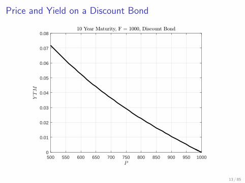
Price and Yield on a Discount Bond

500 550 600 650 700 750 800 850 900 950 1000P

0

0.01

0.02

0.03

0.04

0.05

0.06

0.07

0.08Y

TM

10 Year Maturity, F = 1000, Discount Bond

13 / 85

YTM on a Coupon Bond

I Suppose a bond has a face value of $100 and a maturity ofthree years

I It pays coupon payments of $10 in years t + 1, t + 2, andt + 3 (the coupon rate in this example is 10 percent)

I The face value is paid off after period t + 3

I The period t price of the bond is $100

I The YTM solves:

100 =10

1 + i+

10

(1 + i)2+

10

(1 + i)3+

100

(1 + i)3

I Which works out to i = 0.1

I More generally, for an n period maturity:

P =n

∑j=1

C

(1 + i)j+

FV

(1 + i)n

14 / 85

Price and Yield on a Coupon Bond

800 850 900 950 1000 1050 1100 1150 1200P

0.08

0.085

0.09

0.095

0.1

0.105

0.11

0.115

0.12

0.125

0.13Y

TM

30 Year Maturity, F = 1000, Coupon Rate = 10 Percent

15 / 85

Coupon Rate vs. Yield

I In the example two slides ago, the coupon rate (10 percent)and yield (10 percent) are the same

I In general, this is not going to be true

I Will only be true if the bond “sells at par” – meaning the priceof the bond equals the face value. If bond sells at a discountto face value, yield is greater than coupon rate and vice-versa

I Coupon rate is not the same thing as “the” interest rate!

16 / 85

Perpetuities

I Perpetuities (also called “consols”) are like coupon bonds,except they have no maturity date

I Here, the relationship between price, yield, and couponpayments works out cleanly and is given by:

i =C

P

I For a coupon bond with a sufficiently long maturity, this is areasonable approximation to the bond’s YTM (because thePDV of the face value after many years is close to zero)

I This expression is also sometimes called the current yield asan approximation to the YTM on a coupon bond

17 / 85

Price and Yield on a Perpetuity

1000 1100 1200 1300 1400 1500 1600 1700 1800 1900 2000P

0.05

0.055

0.06

0.065

0.07

0.075

0.08

0.085

0.09

0.095

0.1Y

TM

Perpetuity, C = 100

18 / 85

Observations

I Several observations are noteworthy from the previous slides:

1. The bond price and yield are negatively related. This is truefor all types of bonds. Bond prices and interest rates move inopposite directions

2. For discount bonds, we would not expect price to be greaterthan face value – this would imply a negative yield

3. For a coupon bond, when the bond is priced at face value, theyield to maturity equals the coupon rate

4. For a coupon bond, when the bond is priced less than facevalue, the YTM is greater than the coupon rate (andvice-versa)

19 / 85

Yields (Interest Rates) and ReturnsI Returns and yields (interest rates) are in general not the same

thingI Rate of return: cash flow plus new security price, divided by

current priceI Useful way to think about it (terminology here is related to

equities): “dividend rate plus capital gain,” where capital gainis the change in the security’s price

I The return on a coupon bond held from t to t + 1 is:

R =C + Pt+1 − Pt

Pt

I Or:

R =C

Pt︸︷︷︸Current Yield

+Pt+1 − Pt

Pt︸ ︷︷ ︸Capital Gain

I Return will differ from current yield (approximation to YTM)if bond prices fluctuates in unexpected ways

20 / 85

Discount Bond

I Suppose that you hold a discount bond with face value $1000,a maturity of 30 years, and a current yield to maturity of 10percent

I The current price of this bond is 10001.130

= 57.31.

I Suppose that interest rates stay the same after a year. Thenthe bond has a price of 1000

1.129= 63.04

I Since there is no coupon payment, your one year holdingperiod return (holding period refers to length of time you holdthe security) is just the capital gain:

R =Pt+1 − Pt

Pt=

63.04− 57.31

57.31= 0.10

I If interest rates do not change, then the return and the yieldto maturity are the same thing

21 / 85

Interest Rate Risk

I Continue with the same setup

I But now suppose that interest rates go up to 15 percent inperiod t + 1 and are expected to remain there

I Then the price of the bond in period t + 1 will be:10001.1529

= 17.37 – i.e. the bond price falls

I Your return is then:

R =Pt+1 − Pt

Pt=

17.37− 57.31

57.31= −0.69

I On a discount bond, an increase in interest rates exposes youto capital loss

I True more generally for a coupon bond – while you knowcurrent yield at time of investment, capital gain is unknown

I What we call interest rate risk (close related concept isduration risk)

22 / 85

Return and Time to Maturity, Coupon Bond

0 5 10 15 20 25 30Time to Maturity

-0.25

-0.2

-0.15

-0.1

-0.05

0

0.05

0.1R

Interest Rate Increase from 10 to 15 Percent, 10 Percent Coupon Rate, F = 1000

23 / 85

ObservationsI Return and initial YTM are equal if the holding period is the

same as time to maturity (1 period). The capital gain issimply the face value (which is fixed) minus the initial price

I Increase in interest rates results in returns being less thaninitial yield

I Reverse is trueI Return is more affected by interest rate change the longer is

the time to maturityI If you hold the bond until maturity, your return is locked in at

initial YTMI Concept of return is relevant even if you do not sell the bond

and realize the capital loss. There is an opportunity cost – ifinterest rates rise, had you not locked yourself in on a longmaturity bond you could have purchased a bond in the futurewith a higher yield

I Longer maturity bonds are therefore riskier than shortmaturity bonds

24 / 85

Determinants of Bond Prices (and Interest Rates)

I We’ve talked about specifics of bonds

I But what determines prices (and hence yields)?I Two related approaches:

I Conceptual (Mishkin): demand and supplyI Micro-founded (GLS): explicit consumption-saving

maximization problem

I For simplicity, think of all bonds as discount bonds (makes lifeeasier)

25 / 85

Conceptual Approach: Portfolio Choice

I A bond (or any asset) is a way to transfer resourcesintertemporally

I Demand for a bond is based on the following factors:

1. Wealth/income: assets are normal goods, so the more wealth,the more you want to hold at every price

2. Expected returns: you hold assets to earn returns. The higherthe expected return, the more of it you demand

3. Risk: assume agents are risk averse. Holding expected returnconstant, you would prefer a less risky return. The more riskyan asset is, the less of it you demand

4. Liquidity: refers to the ease with which you can sell an assetand uncertainty over future price fluctuations. The more liquidit is, the more attractive it is to hold (it’s easier to sell at aknown price if you need to raise cash in a pinch)

26 / 85

Demand for Bonds

I How does the demand for bonds vary with the price of bonds?

I As the price goes down, the yield goes up

I Therefore, holding everything else fixed, the expected return(yield) on holding a bond goes up as the price falls

I Therefore, demand slopes down

I Demand will shift (change in quantity demanded for a givenprice) with changes in other factors

27 / 85

Bond Demand

𝑃

𝑄

𝐷

Shifts right if: (i) Wealth goes up (ii) Expected return goes up (iii) Riskiness goes down (iv) Liquidity goes up

28 / 85

Supply of Bonds

I Issuers of bonds are borrowers. You are issuing a bond to raisefunds in the present to be paid back in the future

I Recall that bond prices move opposite interest rates

I As the bond price increases, the yield decreases

I Therefore, at a higher bond price, the cost of borrowing islower

I So there will be more supply of bonds at a higher price –supply slopes up

I Changes in other factors, holding price fixed, will cause thesupply curve to shift

29 / 85

Bond Supply

𝑃

𝑄

𝑆

Shifts right if: (i) Expected profitability

goes up (ii) Expected inflation

goes up (iii) Government deficit

goes up

30 / 85

Bond Market Equilibrium

𝑃𝑃

𝑄𝑄

𝑆𝑆

𝐷𝐷

𝑃𝑃∗

𝑄𝑄∗

31 / 85

An Increase in Risk

𝑃𝑃

𝑄𝑄

𝑆𝑆

𝐷𝐷

𝑄𝑄0∗

𝐷𝐷′

𝑄𝑄1∗

𝑃𝑃0∗

𝑃𝑃1∗

An increase in perceived risk reduces demand for bonds, resulting in lower bond prices and higher interest rates

32 / 85

An Increase in Liquidity

𝑃𝑃

𝑄𝑄

𝑆𝑆

𝐷𝐷

𝑄𝑄0∗

𝐷𝐷′

𝑄𝑄1∗

𝑃𝑃0∗

𝑃𝑃1∗ An increase in liquidity increases demand, raises bond prices, and therefore lowers interest rates

33 / 85

An Increase in Expected Future Interest Rates

𝑃𝑃

𝑄𝑄

𝑆𝑆

𝐷𝐷

𝑄𝑄0∗

𝐷𝐷′

𝑄𝑄1∗

𝑃𝑃0∗

𝑃𝑃1∗

An increase in expected future interest rates lowers expected bond returns. This shifts the demand curve in, resulting in a lower price and higher yield

34 / 85

An Increase in Government Budget Deficit

𝑃𝑃

𝑄𝑄

𝑆𝑆

𝐷𝐷

𝑄𝑄0∗ 𝑄𝑄1∗

𝑃𝑃0∗

𝑃𝑃1∗

An increase in government budget deficits causes the supply of bonds to shift to the right, resulting in lower bond prices and higher interest rates

𝑆𝑆′

35 / 85

Micro-Founded Approach

I Household lives (at least) two periods: t and t + 1

I Can purchase/sell one period discount bonds at PBt

I Assume no uncertainty

U = u(Ct) + βu(Ct+1)

I Budget constraints:

Ct + PBt Bt = Yt

Ct+1 = Yt+1 + Bt

I You hold/issue Bt to smooth consumption relative to income

36 / 85

Euler Equation and Stochastic Discount Factor (SDF)

I Optimization yields an Euler equation:

PBt =

βu′(Ct+1)

u′(Ct)

I Right hand side is known as stochastic discount factor, mt,t+1

I General asset pricing condition:

PAt = E

[mt,t+jD

At+j

]I Where E is expectations operator (allows for uncertainty over

future), A indexes an asset, DAt+j is the cash flow generated by

the asset in period t + j , and mt,t+j =βju′(Ct+j )u′(Ct )

is the

stochastic discount factor

I If we abstract from supply (assume bonds in zero net supply),then Ct = Yt and this determines equilibrium bond prices(and hence yields)

37 / 85

Prices and Yields

I If operating in endowment economy with fixed bond supply,Euler equation determines bond prices (and hence yields)

I Yield on one period discount bond:

1 + iB,t =1

PBt

I Useful to compare assets according to yields instead of prices.Why? Suppose you have a discount bond that pays out 2 int + 1 (label this D) but is otherwise identical to B

I Price of asset D will be double price of B. But yields areidentical:

1 + iB,t = 1 + iD,t =1

PBt

=2

PDt

I Comparing yields puts assets with different levels of cash flowon “equal footing”

38 / 85

Different Bond Characteristics

I Bonds with the same cash flow details (e.g. discount bonds)nevertheless often have very different yields

I Why is this?I Aside from details about cash flows, bonds differ principally

on two dimensions:

1. Default risk2. Time to maturity

I Both generate uncertainty

39 / 85

Default Risk

I Default occurs when the borrower decides to not make goodon a promise to pay back all or some of his/her outstandingdebts

I We think of federal government bonds as being (essentially)default-free: since government can always “print” money,should not explicitly default (though monetization of debt iseffectively form of default)

I Corporate (and state and local government) bonds do havesome default risk

I Rating agencies: Aaa is highest rated, then Bs, then Csmeasure credit risk of lenders

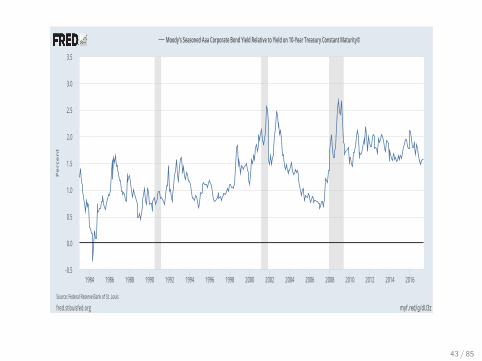
I Risk premium: difference (i.e. spread) between yield onrelatively more risky debt (e.g. Aaa corporate debt) and lessrisk debt (e.g. government debt), assuming same time tomaturity

40 / 85

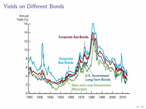
Yields on Different Bonds

41 / 85

Observations

I We see more or less exactly the pattern we would expect fromour demand/supply analysis – riskier bonds have higher yields

I You demand a higher yield (expected return) to becompensated for taking on more risk

I Obvious exception: municipal bonds

I Why? Interest income on these bonds is exempt from federaltaxes, which makes their expected returns higher, andtherefore drives up price (and drives down yield)

I Important: interesting time variation in spreads (see nextcouple of slides)

42 / 85

myf.red/g/dU3z

-0.5

0.0

0.5

1.0

1.5

2.0

2.5

3.0

3.5

1984 1986 1988 1990 1992 1994 1996 1998 2000 2002 2004 2006 2008 2010 2012 2014 2016

fred.stlouisfed.orgSource:FederalReserveBankofSt.Louis

Moody'sSeasonedAaaCorporateBondYieldRelativetoYieldon10-YearTreasuryConstantMaturity©

Percent

43 / 85

myf.red/g/dTre

1

2

3

4

5

6

7

1988 1990 1992 1994 1996 1998 2000 2002 2004 2006 2008 2010 2012 2014 2016

fred.stlouisfed.orgSource:FederalReserveBankofSt.Louis

Moody'sSeasonedBaaCorporateBondYieldRelativetoYieldon10-YearTreasuryConstantMaturity©

Percent

44 / 85

Countercyclical Default Risk

I It stands to reason that default risk ought to be high wheneconomy is in recession

I When default risk is high, we might expect a “flight tosafety”: reduces demand for risky bonds and increasesdemand for riskless bonds, which moves credit spread up

I This is consistent with what we see in the previous slides:credit spreads tend to rise during recessions

45 / 85

Flight to Safety

𝑃𝑃 𝑃𝑃 𝑆𝑆 𝑆𝑆

𝐷𝐷 𝐷𝐷

𝑄𝑄 𝑄𝑄

𝑃𝑃0 𝑃𝑃0

𝑄𝑄0 𝑄𝑄0

𝐷𝐷′

𝐷𝐷′

Corporate Bonds Government Bonds

𝑃𝑃1

𝑃𝑃1

𝑄𝑄1 𝑄𝑄1

46 / 85

Yields During Great Recession

2.003.004.005.006.007.008.009.00

10.00

Yields and the Great Recession

Baa Aaa 10 Yr Treasury

47 / 85

A Micro-Founded Approach

I Household lives for two periods. Receives endowment ofincome. Future endowment is uncertain

I Can save in period t either via discount bonds B1,t or B2,t .B1,t is risk-free. B2,t might default (completely, so pays backno principal)

I Current endowment is known. Future endowment is uncertain.Four possible states of the world in t + 1:

State 1 : Yt+1 = Y ht+1, risky bond pays

State 2 : Yt+1 = Y ht+1, risky bond defaults

State 3 : Yt+1 = Y lt+1, risky bond pays

State 4 : Yt+1 = Y lt+1, risky bond defaults

I Assume probabilities are p1, p2, p3, and p4, withp1 + p2 + p3 + p4 = 1.

48 / 85

Expected Utility and Budget Constraints

I Household wishes to maximize expected utility:

U = u(Ct ) + β E[u(Ct+1)]

= u(Ct ) + β [p1u(Ct+1(1)) + p2u(Ct+1(2)) + p3u(Ct+1(3)) + p4u(Ct+1(4))]

I Budget constraints must hold in each state of the world:

Ct + PB1,tB1,t + PB

2,tB2,t = Yt

Ct+1(1) = Y ht+1 + B1,t + B2,t

Ct+1(2) = Y ht+1 + B1,t

Ct+1(3) = Y lt+1 + B1,t + B2,t

Ct+1(4) = Y lt+1 + B1,t

49 / 85

Facts About Expectations Operators

I Just probability-weighted sum of outcomes:

E[Xt+1] = p1Xt+1(1) + p2Xt+1(2) + · · ·+ pnXt+1(n)

I Useful facts:

E[f (Xt+1)] 6= f (E[Xt+1]) unless f (·) is linear

E[aXt+1)] = aE[Xt+1]

E[Xt+1 + Yt+1] = E[Xt+1] + E[Yt+1]

∂ E[f (Xt+1)]

∂Xt+1= E[f ′(Xt+1)]

E[Xt+1Yt+1] = E[Xt+1]E[Yt+1] + cov(Xt+1,Yt+1)

cov(Xt+1,Yt+1) = E [(Xt+1 −E(Xt+1)) (Yt+1 −E(Yt+1))]

50 / 85

Optimization in an Endowment Economy

I Risk-free bond:

P1,t = E

[βu′(Yt+1)

u′(Yt)

]I Risky bond:

P2,t = E

[βu′(Yt+1)

u′(Yt)D2t+1

]I Where D2

t+1 is the payout on the risky bond (either 1 or 0).Yields:

1 + i1,t =1

PB1,t

=u′(Yt)

E[βu′(Yt+1)]

1 + i2,t =E[D2

t+1]

PB2,t

=E[D2

t+1]u′(Yt)

E[βu′(Yt+1)D2t+1]

51 / 85

Risk Premium

I Ratio of yields is:

1 + i2,t1 + i1,t

=E[D2

t+1]E[u′(Yt+1)]

E[D2t+1u

′(Yt+1)]

I One would be tempted to “distribute” the expectationsoperator and conclude this is 1 (so no difference in yields)

I But in general cannot do this

I After using properties of expectations, one gets:

i2,t − i1,t ≈ −cov(D2

t+1, u′(Yt+1))

E[D2t+1u

′(Yt+1)]

I Risk premium depends on covariance of bond payout withu′(Yt+1), not variance of payout per se

52 / 85

Intuition

I Assuming u′′(·) < 0 (what we call risk averse), you desire tosmooth consumption

I Both across time as well as across states

I Periods where income is high: you want to save to giveyourself resources in other periods

I For assets, you like assets that have comparatively highpayouts in periods where income is low (i.e. periods whereu′(Yt+1) is high, so consumption is highly valued). This helpsyou smooth consumption across states

I Dislike assets that don’t help you do this

I Assets most likely to default in “bad” periods (where u′(Yt+1)is high): you demand a higher yield to hold them (lower price)

I Countercyclical default risk: source of bond risk premia

53 / 85

Uncertainty and the Risk Premium

I Y ht+1 = 1.1, Y l

t+1 = 0.9, Yt = 1, β = 0.95, log utility

I Recall: state 1: income high, bond pays; state 2: income high,bond defaults; state 3, income low, bond pays; state 4:income low, bond defaults

Probabilities E(D) E(Yt+1) E(D2t+1 | Y h

t+1) E(D2t+1 | Y l

t+1) i2,t − i1,t

p1 = p2 = p3 = p4 = 0.25 0.5 1 0.5 0.5 0.00p1 = 0.5, p2 = p3 = 0, p4 = 0.5 0.5 1 1 0 0.12p1 = p4 = 0, p2 = p3 = 0.5 0.5 1 0 1 -0.09p1 = 0.4, p2 = 0.1, p3 = 0.1, p4 = 0.4 0.5 1 0.8 0.2 0.07

I If default is mostly likely in periods where income is low, youdemand a higher yield relative to the risk-free bond

I In principal risk premium could be negative if default is mostlikely when income is high

I Also, risk premium doesn’t depend on uncertainty over defaultper se

54 / 85

Term Structure of Interest Rates

I Bonds with otherwise identical cash flows and riskcharacteristics can have different times to maturity (or justmaturities, for short)

I Think about (default) riskless Treasury securities withdifferent maturities

I Treasury bills: discount bonds with maturities of 4, 13 (threemonth T-Bill), 26, or 52 week maturities

I Treasury notes: coupon bonds with maturities of 2, 3, 5, 7 and10 years

I Treasury bonds: coupon bonds with maturities > 10 years

I How do yields vary with time to maturity for a bond withotherwise identical default characteristics?

I A plot of yields on bonds against the time to maturity isknown as a yield curve

55 / 85

56 / 85

0

1

2

3

4

5

6

1 mo 3 mo 6 mo 1 yr 2 yr 3 yr 5 yr 7 yr 10 yr 20 yr 30 yr

Yie

ld t

o M

atu

rity

Time to Maturity

2017

2014

2011

2009

2008

2007

57 / 85

Observations

I The following observations can be made from previous twopictures

1. Yields on bonds of different maturities tend to move together2. Yield curves are upward-sloping most of the time

I The slope of the yield curve is often predictive of recession.Flat or downward-sloping (“inverted”) yield curves oftenprecede recessions

3. When short term interest rates are low, yield curves are morelikely to be upward-sloping

58 / 85

Yield Curves Prior to Recent Recessions

0

1

2

3

4

5

6

7

8

9

3 mo 6 mo 1 yr 2 yr 3 yr 5 yr 7 yr 10 yr 30yr

Yie

ld t

o M

atu

rity

Time to Maturity

2007

2000

1990

59 / 85

Theories of the Yield Curve

I Main theories of the term structure:

1. Expectations hypothesis2. Segmented markets3. Liquidity premium theory

I Expectations hypothesis: bonds of different maturities areperfect substitutes

I Segmented markets: bonds with different maturities are notsubstitutes

I Liquidity premium: bonds with different maturities areimperfect substitutes

I Essentially expectations hypothesis + uncertainty, wherelonger maturity bonds are riskier (i.e. less liquid) than shortmaturity bonds because their prices fluctuate more

60 / 85

Expectations HypothesisI Expectations hypothesis: the yield on a long maturity bond is the

average of the expected yields on shorter maturity bonds

I For example, suppose you consider 1 and 2 year bonds

I The yield on a 1 year bond is 4 percent; you expect the yield on a 1year bond one year from now to be 6 percent

I Then the yield on a two year bond ought to be 5 percent(0.5× (4 + 6) = 5)

I Why? If you buy a two 1 year bonds in succession, your yield overthe two year period is (approximately, ignoring compounding) 10percent: (1 + 0.04)× (1 + 0.06)− 1 = 0.1024 ≈ 0.10

I If the 2 and 1 year bonds are perfect substitutes, the yield on thetwo year bond has to be the same: (1 + i)2 = 0.1⇒ i ≈ 0.05

I Demand and supply: if you expect future short yields to rise, this

lowers expected profitability of long term bonds in the present,

reducing demand, driving down price, and driving up yield: current

long term yield tells you something about expected future short

term yields

61 / 85

Microfoundations of Expectations Hypothesis

I Suppose a household lives for three periods, receiving anexogenous endowment of income in each period

I In period t, can purchase one or two period maturity discountbonds:

Ct + Pt,t,t+1Bt,t,t+1 + Pt,t,t+2Bt,t,t+2 = Yt

I Subscript notation. First subscript denotes date ofobservation (i.e. period t is the “present”). Second subscriptdenotes date of issuance, third subscript denotes date ofmaturity. So Bt,t,t+1 is the quantity of a bond purchased inperiod t (first subscript), that was issued in period t (secondsubscript), which matures in t + 1 (third subscript)

62 / 85

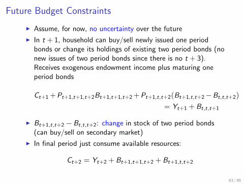
Future Budget Constraints

I Assume, for now, no uncertainty over the future

I In t + 1, household can buy/sell newly issued one periodbonds or change its holdings of existing two period bonds (nonew issues of two period bonds since there is no t + 3).Receives exogenous endowment income plus maturing oneperiod bonds

Ct+1+Pt+1,t+1,t+2Bt+1,t+1,t+2+Pt+1,t,t+2(Bt+1,t,t+2−Bt,t,t+2)

= Yt+1 + Bt,t,t+1

I Bt+1,t,t+2 − Bt,t,t+2: change in stock of two period bonds(can buy/sell on secondary market)

I In final period just consume available resources:

Ct+2 = Yt+2 + Bt+1,t+1,t+2 + Bt+1,t,t+2

63 / 85

Preferences and Optimality Conditions

I Lifetime utility:

U = lnCt + β lnCt+1 + β2 lnCt+2

I Optimality conditions:

Bt,t,t+1 : Pt,t,t+1u′(Ct) = βu′(Ct+1)

Bt,t,t+2 : Pt,t,t+2u′(Ct) = βPt+1,t,t+2u

′(Ct+1)

Bt+1,t+1,t+2 : Pt+1,t+1,t+2u′(Ct+1) = βu′(Ct+2)

Bt+1,t,t+2 : Pt+1,t,t+2u′(Ct+1) = βu′(Ct+2)

I Note: must have Pt+1,t,t+2 = Pt+1,t+1,t+2. Price of bonddepends on time to maturity not date of issuance

64 / 85

Combining These TogetherI If we combine these FOC, we get:

Pt,t,t+2 = Pt,t,t+1 × Pt+1,t+1,t+2

I Price of long bond is product of short maturity bond pricesI Yield is discount rate which equates bond price to present

discounted value of cash flows:

1

(1 + it,t+2)2=

1

1 + it,t+1

1

1 + it+1,t+2

I Note: don’t need to keep track of issuance date, just date ofobservation and maturity date

I Approximately:

it,t+2 ≈1

2[it,t+1 + it+1,t+2]

I Extends to n period maturity:

it,t+n ≈1

n[it,t+1 + it+1,t+2 + · · ·+ it+n−1,t+n]

65 / 85

Forward Rates

I Expectations hypothesis can be used to infer marketexpectations of future short maturity interest rates

I How? By using present yields of bonds on different maturities

I We call these forward rates:

iet+1,t+2 = 2it,t+2 − it,t+1

iet+2,t+3 = 3it,t+3 − 2it,t+2

...

iet+n−1,t+n = nit,t+n − (n− 1)it,t+n−1

66 / 85

Implied 1 Year Ahead Forward Rate

0

1

2

3

4

5

6

7

8

9

10

1991 1994 1997 2000 2003 2006 2009 2012 2015

Forward Rate 1 Yr Ago

Realized 1 Yr Rate

67 / 85

Implied 2 Year Ahead Forward Rate

0

1

2

3

4

5

6

7

8

9

10

1992 1995 1998 2001 2004 2007 2010 2013 2016

Forward Rate 2 Yrs Ago

Realized 1 Yr Rate

68 / 85

Evaluating the Expectations Hypothesis

I Expectations hypothesis can help make sense of several facts:

1. Long and short term rates tend to move together. If currentshort term rates are low and people expect them to stay lowfor a while (interest rates are quite persistent), then long termyields will also be low

2. Why a flattening/inversion of yield curve can predictrecessions. If people expect economy to go into recession, theywill expect the Fed to lower short term interest rates in thefuture. If short term interest rates are expected to fall, thenlong term rates will fall relative to current short term rates,and the yield curve will flatten.

I Where the expectations hypothesis fails: why are yield curvesalmost always upward-sloping? If interest rates aremean-reverting, then the typical yield curve ought to be flat,not upward-sloping

69 / 85

Segmented Markets

I Segmented markets: household heterogeneityI Some households like long maturity debt, others prefer short

maturity debtI e.g. investors match maturity to their retirement horizon

I If very risk averse investors prefer short maturity bonds, thesewill tend to on average have low yields

I In contrast, if less risk averse investors prefer longer maturitybonds, these will tend to have higher yields

I This can account for why yield curves are typicallyupward-sloping

I But because there is no relation between short and long termyields, it fails to make sense of other facts about the termstructure

70 / 85

Liquidity Premium TheoryI Segmented markets hypothesis cannot explain why interest

rates of different maturities tend to move together, or accountfor why you can predict future short term rates from longterm yields

I Liquidity premium theory: essentially expectations hypothesiswith uncertainty

I Bonds of different maturities are substitutes, but not perfectsubstitutes

I Why? Long maturity bonds are riskier – they bear interestrate risk where bond prices will fluctuate

I Savers demand compensation for this riskI Relationship between long and short rates:

it,t+n =it,t+1 + iet+1,t+2 + . . . iet+n−1,t+n

n︸ ︷︷ ︸Expectations Hypothesis

+ ln,t︸︷︷︸Liquidity Premium

I The liquidity premium, ln,t (also called term premium), isincreasing in the time to maturity

71 / 85

72 / 85

Microfoundations of Liquidity Premium

I Same setup as before, except future endowments are uncertain

I Assume no default risk

I Endowment in t + 1 or t + 2 can be high or low –Yt+1 = Y h

t+1 or Y lt+1 (and similarly for Yt+2)

I Assume probability is p of high income draw and 1− p of lowendowment; same in t + 1 and t + 2

I Budget constraints (significantly) more complicated – twostates of the world in t + 1, and essentially four states of theworld in t + 2

I Why four in t + 2? Because consumption in t + 2 depends ondecisions made in t + 1. So 2× 2 = 4.

I Objective function is to maximize expected lifetime utility

I We will skip a bunch of (nasty) steps but it is laid out for youin GLS Ch. 33

73 / 85

Optimality Conditions

I Optimality conditions look the same as above, but withexpectations operators

I Once again, price of bonds in t + 1 depends only on time tomaturity, not date of issuance

I Using these facts, we get:

Pt,t,t+1u′(Ct) = β E[u′(Ct+1)]

Pt,t,t+2u′(Ct) = β E[Pt+1,t+1,t+2u

′(Ct+1)]

I Intuitive MB = MC interpretation, just with expectationsoperators

74 / 85

Combining These Conditions

I Divide second FOC by first and re-arrange to get:

Pt,t,t+2 = Pt,t,t+1E[Pt+1,t+1,t+2u

′(Ct+1)]

E[u′(Ct+1)]

I One is tempted to “distribute” the expectations operator inthe numerator, which would yield:

Pt,t,t+2 = Pt,t,t+1 E[Pt+1,t+1,t+2]

I This would be the natural analog of what we just had,allowing for uncertainty over the future bond price

I But in general you cannot do this unless (i) u′(Ct+1) is aconstant (i.e. u(·) is linear) or (ii) Pt+1,t+1,t+2 is uncorrelatedwith u′(Ct+1)

I Note: this is very much like what we saw when studying riskpremia – you cannot “distribute” the expectations operatorthrough a product

75 / 85

Re-Arranging

I Can write this expression as:

Pt,t,t+2 = Pt,t,t+1 E[Pt+1,t+1,t+2]E[Pt+1,t+1,t+2u

′(Ct+1)]

E[Pt+1,t+1,t+2]E[u′(Ct+1)]

I If income equals consumption (bonds in zero net supply), weget:

Pt,t,t+2 = Pt,t,t+1 E[Pt+1,t+1,t+2]︸ ︷︷ ︸Expectations Hypothesis

(1 +

cov(Pt+1,t+1,t+2, u′(Yt+1))

E[Pt+1,t+1,t+2]E[u′(Yt+1)]

)︸ ︷︷ ︸

Term Premium

I We would expect covariance term to be negative

I When Yt+1 is low, u′(Yt+1) is high and demand for oneperiod bonds is low (people don’t want to save), soPt+1,t+1,t+2 is low

I Negative covariance ⇒ two period bond trades at a discountrelative to what expectations hypothesis would predict

76 / 85

Prices to Yields

I Written in terms of yields, approximately we get:

(1+ it,t+2)2 = (1+ it,t+1)E[1+ it+1,t+2]

(1 +

cov(Pt+1,t+1,t+2, u′(Yt+1))

E[Pt+1,t+1,t+2]E[u′(Yt+1)]

)−1I Which is approximately:

it,t+2 ≈1

2

[it,t+1 + iet+1,t+2

]+

1

2tpt

I Where:

tpt = − ln

(1 +

cov(Pt+1,t+1,t+2, u′(Yt+1))

E[Pt+1,t+1,t+2]E[u′(Yt+1)]

)I Where we would expect tpt > 0 if cov(·) < 0

77 / 85

General Case

I For an n period bond, we get:

it,t+n ≈1

n

[it,t+1 + iet+1,t+2 + . . . iet+n−1,t+n

]+

n− 1

ntpt

I Where tpt is exactly the same as before – based on covariancebetween future one period bond price and future marginalutility

I So as n gets bigger, n−1n tpt gets bigger (at a decreasing rate)

I This delivers positive slope of typical yield curve, butexpectations hypothesis logic drives movements in short andlong term yields

78 / 85

A First Look at Quantitative Easing and UnconventionalMonetary Policy

I The interest rates relevant for most investment andconsumption decisions are long term (e.g. mortgage) andrisky (e.g. Baa corporate bond)

I Conventional monetary policy targets short term and risklessinterest rates (e.g. Fed Funds Rate)

I In practice, something like a 10 Year Treasury yield serves as abenchmark interest rate for all other kinds of interest rates –mortgage rates, credit card rates, student loan rates

I These are the rates relevant for economic decisions onspending and saving

I Out theory of bond pricing helps us understand theconnection between the these different kinds of interest rates

79 / 85

Monetary Policy in Normal Times

I Think of a world where the liquidity premium theory holds

I A central bank lowers (raises) short term interest rates and isexpected to keep these low (high) for some time

I This ought to also lower (raise) longer term rates to theextent to which longer term rates are the average of expectedshorter term rates

I Holding risk factors constant, substitutability between bondsmeans that riskier yields also ought to fall (increase)

I Simulation:I Consider 1 period, 10 year, 20 year, and 30 year bondsI Fixed liquidity premia of 1, 2, and 3I Short term rate is cut from 4 to 3 persistentlyI Simulate yields for 30 quarters

80 / 85

Theoretical Simulation

0 10 20 30Quarters

3

4

5

6

7

8

Yield

s

No Cut

Short Rate10 Year20 Year30 Year

0 10 20 30Quarters

3

4

5

6

7

8

Yield

s

Rate Cut

81 / 85

Monetary Loosening and Tightening in Historical Episodes

5.0000

6.0000

7.0000

8.0000

9.0000

10.0000

11.0000

FFR

AAA

Baa

Mortgage

10 Yr Treasury2.0000

3.0000

4.0000

5.0000

6.0000

7.0000

8.0000

9.0000

10.0000

FFR

Aaa

Baa

Mortgage

10 Yr Treasury

82 / 85

Monetary Loosening and Tightening in Historical Episodes

0.00001.00002.00003.00004.00005.00006.00007.00008.00009.0000

20

00

-1

2-0

1

20

01

-0

1-0

1

20

01

-0

2-0

12

00

1-0

3-0

1

20

01

-0

4-0

12

00

1-0

5-0

1

20

01

-0

6-0

12

00

1-0

7-0

1

20

01

-0

8-0

1

20

01

-0

9-0

12

00

1-1

0-0

1

20

01

-1

1-0

12

00

1-1

2-0

1

20

02

-0

1-0

1

20

02

-0

2-0

1

FFR

Aaa

Baa

Mortgage

10 Yr Treasury0.0000

1.0000

2.0000

3.0000

4.0000

5.0000

6.0000

7.0000

8.0000

FFR

Aaa

Baa

Mortgage

10 Yr Treasury

83 / 85

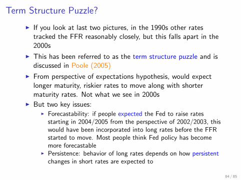
Term Structure Puzzle?

I If you look at last two pictures, in the 1990s other ratestracked the FFR reasonably closely, but this falls apart in the2000s

I This has been referred to as the term structure puzzle and isdiscussed in Poole (2005)

I From perspective of expectations hypothesis, would expectlonger maturity, riskier rates to move along with shortermaturity rates. Not what we see in 2000s

I But two key issues:I Forecastability: if people expected the Fed to raise rates

starting in 2004/2005 from the perspective of 2002/2003, thiswould have been incorporated into long rates before the FFRstarted to move. Most people think Fed policy has becomemore forecastable

I Persistence: behavior of long rates depends on how persistentchanges in short rates are expected to

84 / 85

Unconventional Monetary Policy

I In a world where Fed Funds Rate is at or very near zero,conventional monetary loosening isn’t on the table

I Unconventional monetary policy:

1. Quantitative Easing (or Large Scale Asset Purchases):purchases of longer maturity government debt or risky privatesector debt. Idea: raise demand for this debt, raise price, andlower yield. See here

2. Forward Guidance: promises to keep future short term interestrates low. Idea is to work through expectations hypothesis andto lower long term yields immediately. See here

I Ben Bernanke: “The problem with quantitative easing is thatit works in practice but not in theory”

I Under expectations hypothesis, cannot affect long term yieldswithout impacting path of short term yields

I Not clear why it ought to be able to impact liquidity/termpremium, which depends on a covariance term

I Segmented markets?

85 / 85