boosting moving average reversion strategy for online
TRANSCRIPT

Boosting Moving Average Reversion Strategy for OnlinePortfolio Selection: A Meta-Learning Approach
Lin Xiao1, Zhang Min2, Zhang Yongfeng3, Gu Zhaoquan4, Liu Yiqun2, and Ma Shaoping2
1 Institute of Interdisciplinary Information Sciences, Tsinghua University, Beijing, China,[email protected];
2 Tsinghua National Laboratory for Information Science and Technology, Department ofComputer Science and Technology, Tsinghua University, Beijing 100084, China,
[email protected]; [email protected]; [email protected] College of Information and Computer Science, University of Massachusetts Amherst, MA
01003, USA, [email protected] Department of Computer Science, HongKong University, HongKong, China,
Abstract. In this paper, we study the online portfolio selection problem fromthe perspective of meta learning for mean reversion. The online portfolio selec-tion problem aims to maximize the final accumulated wealth by rebalancing theportfolio at each time period based on the portfolio prices announced before.Mean Reversion is a typical principle in portfolio theory and strategies that uti-lize this principle achieve the superior empirical performances so far. Howeverthere are some important limits of existing Mean Reversion strategies: First, themean reversion strategies have to set a fixed window size, where the optimal win-dow size can only be chosen in hindsight. Second, most existing mean reversiontechniques ignore the temporal heterogeneity of historical price relatives fromdifferent periods. Moreover, most mean reversion methods suffer from noisesand outliers in the data, which greatly affects the performances. In order to tacklethe limits of previous approaches, we exploit mean reversion principle from ameta learning perspective and propose a boosting method for price relative pre-diction. More specifically, we generate several experts where each expert followsa specific mean reversion policy and predict the final price relatives with metalearning techniques. The sampling of multiple experts involves mean reversionstrategies with various window sizes; while the meta learning technique bringstemporal heterogeneity and stronger robustness for prediction. We adopt onlinepassive-aggressive learning for portfolio optimization with the predicted pricerelatives. Extensive experiments have been conducted on real-world datasets andour approach outperforms the state-of-the-art approaches significantly.
1 Introduction
Online portfolio selection problem aims to allocate the wealth among different assets atdifferent time periods to maximize the long-term wealth. There are two models describ-ing the problem: the Mean-Variance model[19] and Kelly’s Capital Growth model [11].The first model uses a weighted sum of expected return (mean) and risk (variance ofthe return) as a trade-off between the two objectives, and it is suitable for single-periodportfolio selection; the second model sees the problem as a sequential decision problem

2
that aims to maximize the expected return at the end of multiple time periods. Kelly’sCapital Growth model has a nature of online decision making, which is widely adoptedby the studies from AI and Machine Learning researchers.
In online portfolio selection problem, each asset is associated with a price in eachperiod. The ratio of prices between current period and last period is called price relative,which reflects the return of wealth invested on the assets after one period. The agentallocates the wealth among different assets based on their price relatives at differentperiods. Most portfolio selection strategies follow a two-phase scheme: price relativeprediction phase and portfolio optimization phase. The first phase aims to predict theprice relative at next period based on historical data; while the second phase aims tocompute the optimal portfolio given the prediction of price relative.
One common methodology for this problem is Mean Reversion, which assumes theportfolios that perform poorly at current period will perform well next (and vice versa).The methods include PAMR (Passive Aggressive Mean Reversion)[17], CWMR (Confi-dence Weighting Mean Reversion) [15], OLMAR (OnLine Moving Average Reversion)[14]and RMR (Robust Mean Reversion)[9], which adopt the mean reversion idea in differ-ent ways. They achieve superior empirical results in experiments compared with otherstate-of-art methods. This proves the effectiveness of mean reversion policy.
Although PAMR, CWMR and OLMAR achieve good performances, they still facesome difficulties. All existing mean reversion strategies do not fully consider the noisydata and outliers (RMR is proposed to alleviate the problem), which often leads toestimation error (see [20]). Furthermore, the assumption of single-period prediction[17][15] also leads to estimation error, which makes the performance poor. RMR (Ro-bust Mean Reversion)[9] and OLMAR[14] uses multi-period prediction, but the algo-rithm sees each period equally, which ignores the temporal heterogeneity of historicalprice relatives and causes inaccuracy of predictions. We utilize meta learning to ex-ploit the benefit of multi-period prediction and the periods are assigned with weightsaccording to their performances. Moreover, this alleviates the impact of noisy data andoutliers. The results show that our strategy outperforms RMR and OLMAR.
More specifically, in order to utilize multi-period historical data, we generate multi-ple experts for price relative prediction following typical MAR methods. Then we adoptthe meta learning method for price prediction. Each expert is assigned a weight that isupdated according to their performances and a weighted aggregation is used as the finalprediction. Meanwhile, we choose the typical passive-aggressive learning method forportfolio optimization. This method captures the recent portfolio performances and theobjective of enhancing the wealth return at each time period.
The contributions of our work are: first, to our knowledge, we are the first to exploitthe Mean Reversion strategy with meta learning in online portfolio selection problems;second, we make a better use of multiple-period history, which is robust to the outliersand noises in historical data; third, we conduct extensive experiments on real-worlddatasets and achieve superior results compared with other state-of-the-art approaches.
The remainder of the paper is organized as follows: the next section gives a brief in-troduction to the related work; Section 3 formally introduces the online portfolio selec-tion problem while Section 4 introduces some preliminary works about mean reversiontheory and some related concepts. Section 5 proposes BMAR strategy that utilizes meta

3
learning in online portfolio selection problem. Section 6 presents the results of experi-ments conducted on real-world datasets and a thorough comparison with the baselines.The conclusion and the future work are presented in Section 7.
2 Related Work
The study of online portfolio selection problem first concentrates on some benchmarkalgorithms, including Buy and Hold, Best Stock and Constant Rebalanced Portfolios.The Buy and Hold strategy means the agent invests wealth with an initial portfolio andholds it to the end without changing the portfolio. The Best Stock strategy means thatone puts all the wealth on the stock whose performance is best in hindsight. ConstantRebalanced Portfolios is a strategy that rebalances the wealth to a fixed portfolio inall periods. The best CRP strategy which achieves highest accumulated wealth is calledBCRP. BCRP is an optimal strategy if the market is i.i.d. [4]. Successive Constantly Re-balanced Portfolios (SCRP) [5] and Online Newton Step (ONS) [1] implicitly estimatenext price relative via all historical price relatives with a uniform probability. However,both Best Stock and BCRP strategies have to be computed in hindsight.
There are two main categories of algorithms: follow-the-winner approach and follow-the-loser approach. The intuition behind first approach is to track the stock with bestperformance in history and raise the weights in the portfolio of these stocks. Most of theFollow-the-Winner approaches aim to imitate the BCRP strategy: including the univer-sal portfolio selection (UP)[10], Exponential Gradient (EG)[8], follow-the-leader andfollow-the-regularized-leader approaches. However, the prices of assets are unstable,even a good following of winner assets can not guarantee superior performances.
Follow-the-loser approach utilizes a typical assumption of mean reversion [18],which means that the good (poor)-performing assets will perform poor (good) in thefollowing periods. The approaches in this category include Anti-Correlation (Anticor)[2], Passive-Aggressive Mean Reversion (PAMR)[17], Confidence-weighted Mean Re-version (CWMR)[15], OLine Moving Average Reversion (OLMAR)[14] and RobustMean Reversion (RMR)[9]. CRP[4][5] implicitly envolves follow-the-loser approachsince rebalancing the wealth means to transfer the wealth from winning stocks to losingstocks in some extent.
Another important category of the portfolio selection algorithms is pattern-matching,which estimates the portfolio price based on sampled similar historical patterns. Non-parametric kernel based moving window (BK) [7] measures the similarity by kernelmethod. Following the same framework, Nonparametric Nearest Neighbor (BNN) [12]locates the set of price relatives via nearest neighbor methods. [16] proposed Correlation-driven Nonparametric learning (CORN), which measures the similarity via correlation.
Since the mean-reversion technique is widely adopted in financial fields, it is usefulin online learning algorithms as well. Passive Aggressive Mean Reversion (PAMR) [17]and Confidence Weighted Mean Reversion (CWMR) [15] estimate next price relativeas the inverse of last price relative, which is in essence the mean reversion principle.Recently, [14] proposed On-Line Moving Average Reversion (OLMAR), which pre-dicts the next price relative using moving averages and explores the multi-period meanreversion. Robust Mean Reversion is proposed to alleviate the impact of outliers and

4
noises existing in the data. The empirical experiments indicate that OLMAR and RMRoutperforms the other state-of-the-art algorithms. However, most of the Mean Rever-sion algorithms have important limits: first, the mean reversion strategies require toselect a fixed time window for prediction, which can not be easily determined; second,the strategies treat each time period equally in prediction, which ignores the temporalheterogeneity; third, the strategies do not have strong robustness against noises and out-liers. We utilize mean reversion strategies for its good depiction of reality and furtheruse meta learning approach to tackle the limits. A detailed comparison between ourstrategy and existing Mean Reversion strategies is presented in Section. 4.
3 Problem Setting
In this section, we formally introduce the Online Portfolio Selection problem. Assumethat there exist m assets in market, and time is divided into T periods. Each asset i hasa closing price pt,i at period t and pt is denoted as the closing price vector (columnvector for all vectors mentioned): pt = [pt,1, pt,2, ..., pt,m]. xt,i is the price relative thatcaptures the ratio of closing prices between two consecutive periods: xt,i =
pt,ipt−1,i
andxt = [xt,1, xt,2, ..., xt,m] is the price relative vector.
In each period, the market reveals the closing prices of assets and the investor has toassign the capital with a portfolio vector: bt = [bt,1, bt,2, ..., bt,m] where bt,i representsthe proportion of wealth assigned to asset i at time t. We follow the typical assumptionthat no margin/short sale is allowed, therefore bt,i ≥ 0,∀t, i and
∑mi=1 bt,i = 1,∀t. An
investment means to select a portfolio bt from the simplex: {bt,i ≥ 0,∑mi=1 bt,i = 1} at
period t. Usually we assume the portfolio is uniformly distributed in the beginning: b0 =[ 1m , ...,
1m ]. The sequence of portfolios from t1 to t2 is denoted as bt2t1 . Denote the wealth
accumulated at t as Wt, w.l.g. the initial wealth is assumed to be 1: W0 = 1. Thereforegiven the selected portfolio bt at period t, the wealth becomes Wt = Wt−1b
Tt xt =∑m
i=1 bt,ixt,iWt−1 =∏tτ=1 b
Tτ xτ (T is transpose here).
Given the notations and introduction above, the online portfolio selection problemrefers to a sequential decision making problem with periods from t = 1 to t = n. Ineach period, the investor has to decide the portfolio based on historical closing pricesof assets and the market reveals the newest closing price of assets, which leads to thechange of wealth. The investor needs to strategically design portfolios bn1 so that theaccumulated wealth Wn at time t = n is maximized.
We summarize the procedures from the introduction above and formulate the wholeonline portfolio selection process in Alg. 1 as [13].
4 Preliminary
In this section, we briefly introduce the mean reversion principle and how former worksexploit this principle.
4.1 Mean Reversion
In each period, the algorithm tries to estimate the price relatives of assets in price predic-tion phase and compute the portfolio with Passive-Aggressive or Confidence Weighted

5
Algorithm 1 ONLINE PORTFOLIO SELECTION
Input: xn1 : Historical market price relative sequenceOutput: Wt : Final cumulative wealthProcedure:1: Initialize the portfolio b1 = 1
m1, the wealth is initialized as W0 = 1;
2: for t = 1, 2, ..., n do3: Portfolio mannager learns the portfolio bt;4: Market reveals the market price relative xt;5: Portfolio incurs period return wt = bT
t xt and updates cumulative return Wt = Wt−1 ×(bT
t xt);6: Portfolio manager updates the online portfolio selection rules;7: end for;
Learning given the predicted price relatives. The mean reversion principle is reflected inthe first phase by assuming that the poor-performing assets will have good performancesin next periods (and vice versa). Denote the estimated price relative as x̃t and the es-timated closing price as p̃t. PAMR and CWMR assumes that the assets with high/lowprice relatives will have low/high price relatives in next period: x̃t+1 = 1
xt,∀t, which
means p̃t+1
pt= pt−1
pt. Therefore the principle assumes that p̃t+1 = pt−1. Although the
two methods work well, they can not perform consistently on some datasets. There aretwo reasons that lead to this inefficiency: first, the fluctuating prices may contain noisesthat affect the precision of mean reversion principle; second, the single period pricereversion effect may not exist widely as expected.
4.2 Online Moving Average Reversion
The OLMAR (online moving average reversion) principle is proposed to model themean reversion principle with multiple-period historical data. Denote the time windowof OLMAR as w, the closing price pt at period t is assumed to be: p̃t = 1
w
∑t−1τ=t−w pτ .
The price is therefore considered as the average of prices in a time window and the pricerelative becomes: x̃t = pt
pt−1= 1
w (1 + 1xt−1
+ ...+ 1⊗t−1τ=t−w xτ
). This Moving Average
Reversion strategy with time window is denoted as SMAR.Usually, it is assumed that the price at current period is closer to the price at recent
periods due to the continuity of price changes. Therefore the price can be estimated withMAR by adding a decay factor α: p̃t = αpt−1 +(1−αp̃t−1), which results with a pricerelative: x̃t = α + (1 − α) x̃t−1
xt−1. Therefore the decay factor frees the algorithm from
choosing a time window and utilizes the prices from the whole history. This MovingAverage Reversion strategy with time window is denoted as EMAR.
Given the price relative predictions, OLMAR method further utilizes the onlinepassive aggressive learning policy for portfolio optimization, which is also adopted byPAMR. Notice that the choice of time window size and decay factor determines theperformance of this method and can not be pre-defined in hindsight.

6
Table 1. Comparison between our strategy (BMAR) with Existing Mean Reversion Approaches.
Approaches Mean Reversion Multi-Period Robustness Temporal HeterogenityPAMR
√\ \ \
CWMR√
\ \ \OLMAR
√ √\ \
RMR√ √ √
\BMAR
√ √ √ √
4.3 Robust Mean Reversion
RMR uses L1 estimator to estimate the closing prices of assets so that the result-ing price has a better robustness compared to other methods: with a window size ofhistorical periods w, RMR estimates the closing at t by minimizing this objective:∑t−wτ=t−1 ‖p̃t − pτ‖2, and the price relative is estimated as p̃t
pt−1. This estimation is
named as L1 estimator and is relatively more robust to noises.
4.4 Temporal Heterogeneity
The price relatives of different periods are correlated in different extents. Usually, it isassumed that the price at current period is closer to the price at recent periods due tothe continuity of price changes. Meanwhile, the changes of price relatives in some timewindows are more similar than others (which is the foundation of CORN (CORrelation-driven Nonparametric learning) [16]). Therefore, when predicting the price relativesin the future, the algorithm should consider how to make use of the historical timewindows differently.
Given these existing algorithms exploiting Mean Reversion principles, we make acomparison between our approach (Boosting Moving Average Reversion: BMAR) andthese algorithms in Table. 1. The multi-period column shows whether the approachesuse multiple-period historical data for prediction; the Robustness shows whether theapproaches are robust to noises and outliers; the Temporal Heterogenity column showswhether the approaches can utilize the data from different periods Heterogeneously. Thetable shows that our strategy (BMAR) preserves all the good properties, which showsthe superiority.
5 Proposed Strategy: Boosting Moving Average Reversion
Like most methods, we solve the problem with two phases: price relative prediction andportfolio optimization. We first generate a set of experts and each expert is a predictorof the price relative following a mean reversion policy. In each period, each expert firstmakes its predictions on the price relatives in next period; then we compute the cumu-lated losses induced by each expert from their historical predictions and the true pastprice relatives. With the cumulated losses, we compute the weights assigned to each ex-pert following the boosting methods introduced later and make a final prediction. Thenwe use Online Passive-Aggressive learning method to compute an optimized portfolio

7
Fig. 1. BMAR Strategy for Online Portfolio Selection
with the final prediction of price relatives in next period. When the true price relativesare revealed, we can update the cumulated losses of each predictor. The process ofBMAR strategy for online portfolio selection is illustrated in Fig. 1.
5.1 Boosting Moving Average Reversion for Price Relative Prediction
We generate the experts of price relative prediction with different parameters from OL-MAR. Denote the set of experts as E and the SMAR expert with time window w isdenoted as Ew, the EMAR expert with Decaying factor α as Eα.
Uniform Sampling: We generate the experts by sampling the parameters uniformlyfrom the range: w ∼ U(wmin, wmax) and α ∼ U(0, 1). We generate M = wmax −wmin + 1 experts from MAR (w = wmin, wmin + 1, ..., wmax) and N experts fromEMAR (α = {0.1, 0.2, ..., 0.9} when N = 9). Based on the different ways of generat-ing experts, we denote the strategy of generating experts with time window as BMAR-1and the strategy of generating experts by sampling α as BMAR-2. With the generatedexperts, we use weighted aggregation of their decisions to predict the price relatives atdifferent periods. Each expert represents an approximation of the price relative in nextperiod with a certain time window. By utilizing the predictions of these experts witha weighted scheme, we can induce temporal heterogeneity into our approach and thedetails will be introduced later.
As shown in Theorem 1 later, the regret of our strategy is closely related to thenumber of experts we generate. We will present the influence of expert numbers andsampling methods on the performances in the experiment.
We assume a weighted sum of the experts as the estimator of the price relative:
BMAR−1 : x̃(t) =
∑i=Ni=1 θi,t−1x̃(t, wi)∑i=N
i=1 θi,t−1
;BMAR−2 : x̃(t) =
∑j=Mj=1 θj,t−1x̃(t, αj)∑j=M
j=1 θj,t−1
(1)

8
where x̃(t, w) and x̃(t, α) are the predicted price relatives of expertEw andEα; θw,t−1
and θα,t−1 are the weights assigned to these experts given their performances untilperiod t− 1.
Denote the loss of expert Ew by period t as l(w, t) and the loss of weighted expert(BMAR) by period t as l(t). The cumulated losses of expertEw and weighted expert byperiod T are denoted as L(w, T ) =
∑t=Tt=1 l(w, t) and L(T ) =
∑t=Tt=1 l(t) respectively.
The difference between the two losses is seen as the regret of weighted expert withrespect to expert Ew: R(w, T ) = L(T )− L(w, T ).
We introduce the weights assigned to the expert, i.e. exponential weights:
θi,t−1 =e−ηRi,t−1∑Nj=1 e
−ηRj,t−1(2)
where η is a nonnegative parameter. Notice that R(w, T ) = L(T ) − L(w, T ), theexponential weights make the predictions simpler:
θi,t−1 =e−ηLi,t−1∑Nj=1 e
−ηLj,t−1(3)
It has been proved that this expert learning procedure guarantees a proper upper boundof regret in prediction, as shown in the theorems from [3]:
Theorem 1. Assume that the loss function is convex in its first argument and takesvalues from [0, 1], then the regret of exponentially weighted average predictor satisfies(N is the number of experts, n is the number of periods and η is the parameter inexponential weights):
L̂n − mini=1,...,N
Li,n ≤lnN
η+nη
2(4)
The details of the proofs can be found in [3] and we omit the details here. Giventhese theorems, we can design loss functions that satisfy the requirements:
l(p̂, y) =1
Nε× ‖p̂− y‖22 (5)
where ε is the constant that rescales l(p̂, y) into [0, 1]. And it is easy to verify thatthe function is convex, which satisfies the requirement of the theorems. Notice that εactually works as coefficients of l(p̂, y) with η, we can simply tune the value of η toadjust the performances, therefore when using this loss function, we do not explicitlyset the value of ε.
Remarks on Robustness: Notice that we do not explicitly model robustness inour prediction, however the utilization of multiple experts involves robustness: if theoutliers and noises causes degradation of the experts’ prediction accuracy, the weightsassigned to these affected experts are lowered, which prevents the final predictions suf-fering from the noises and outliers.
5.2 Portfolio Optimization
Given the predicted price relatives shown in former section, we utilize the passive ag-gressive learning procedure to solve an optimal portfolio. The basic idea of passive

9
aggressive learning is to keep the portfolio the same if the predefined requirement issatisfied, otherwise the portfolio is computed to satisfy the requirement with a minimalchange. More specifically, we formulate the optimization problem as follows:
min. ‖bt − bt−1‖2
s.t. btx̃t ≥ ε, and bt � 0(6)
where ε is the threshold for the return at each period. Usually ε is a constant greaterthan 1 to ensure the return under predicted price relative is increasing. The optimum tothis problem is the portfolio assigned for period t. Notice that if we keep the portfoliosame with that in last period and the return under predicted price relatives still exceedsthe required value, we will keep the portfolios unchanged; otherwise, we will try tominimize the change between current portfolio and that in last period as long as thereturn can exceed the requirement. Since this optimization problem is convex, we canderive the portfolio in a closed form. The solution without considering the nonnegativityconstraint is presented in the following proposition:
bt+1 = bt − αt+1(x̂t+1 − x̄t+1 · 1) (7)
where x̄t+1 = 1d (1̇̂xt+1) denotes the average predicted price relative and αt+1 is the
Lagrangian multiplier calculated as,
αt+1 = min{0, x̂t+1bt − ε‖x̂t+1 − x̄t+1 · 1‖2
} (8)
In order to ensure that the portfolio is non-negative, we project the above portfolio intothe simplex domain as [14].
5.3 Transaction Costs
In this section, we will introduce the transaction cost, which is an important factor inpractical scenarios. In practice, each transaction of wealth from one asset to another ischarged with transaction fees. The transaction cost is imposed by markets, and a port-folios behavior cannot change the properties of transaction costs, such as commissionrates or tax rates. Usually we assume the transaction fee follows a proportional model,which means rebalancing a portfolio incurs transaction costs on every buy and sell op-eration, based upon a transaction cost rate of γ ∈ (0, 1). Therefore the transaction costfor a rebalancing from b̂t−1 to bt is computed as:
γ
2×
m∑i=1
|bt,i − b̂t−1,i| (9)
Therefore the cumulated wealth after n periods becomes:
W γn = W0
n∏t=1
[(bt · xt)× (1− γ
2×
m∑i=1
|bt,i − b̂t−1,i|)] (10)
Notice that the main intuition of Passive-Aggressive portfolio optimization is to keepthe portfolio unchanged unless the requirement can not be satisfied. This avoids unnec-essary rebalancing of wealth among assets and saves the transaction costs induced.

10
6 Experiment
We conduct extensive experiments on several real-world datasets to evaluate the perfor-mances of our strategy and make comparisons with state-of-the-art approaches.
6.1 Experiment Setting
In our experiment, we use the real-world datasets that are frequently used in relatedworks. There are four datasets that contain price relatives of assets from US and Globalmarkets. The time frames of these datasets range from decades to years, which reflectthe performances of both long-term and short-term portfolio selections. The details ofthe datasets are listed in Table. 2. In the experiment, we use the metrics that are adoptedin the literatures for evaluation: i.e. the total wealth achieved at the final period.
Table 2. Statistics of the real-world datasets for experiment.
Dataset Region Time Frame # Periods # AssetsNYSE(O) US Jul.3rd 1962-Dec. 31st 1984 5651 36NYSE(N) US Jan.1st 1985-Jun 30th 2010 6431 23SP500 US Jan.2nd 1998-Jan. 31st 2003 1276 25MSCI Global Apr. 1st 2006-Mar.31st 2010 1043 24
6.2 Comparison Approaches
We select the state-of-art algorithms (most of them have been introduced in the relatedworks) for comparison, including those Benchmark algorithms (Market, Best-Stockand BCRP), follow-the-winner algorithms (UP, EG, ONS), pattern-matching algorithms(Bk, BNN , CORN, Anticor) and all the variants of mean reversion algorithms (PAMR,CWMR, OLMAR, RMR). For all the algorithms above, we choose the parameters withbest performances as reported in related works. Notice that we select some algorithmsthat use information in hindsight for comparison (which are strong baseline algorithms).For the default setting of BMAR, we setW = 8 andN = 9 for BMAR-1 and BMAR-2.The other parameters are chosen as: η = 1, ε = 5 for all datasets.
6.3 Performance Evaluation
We present the cumulative wealth of our strategy and the comparative approaches intable. 3. As shown in the table, our strategy achieves the best performance on alldatasets and outperforms other comparative algorithms significantly on long-term port-folio selection problems, i.e. on NYSE(O) and NYSE(N). Notice that the parameters fitfor each dataset can be different, we also list the best performances of algorithms forcomparison. The results show that the (including best or conventional) performancesachieved by BMAR are better than other comparison algorithms. We also conduct sig-nificance test (following [6]) on the performances and the results are listed in Table.4. The significance tests shown above indicate that the performance of our strategy issignificantly better on all datasets, which is not the consequence of luck. Notice that our

11
Table 3. Cumulative Wealth on four datasets.
Categories Approaches NYSE(O) NYSE(N) SP500 MSCI
BaselinesMarket 14.5 18.06 1.34 0.91Best Stock 54.14 83.51 3.78 1.50BCRP 250.60 120.32 4.07 1.51
Followthe winner
UP 26.68 31.49 1.62 0.92EG 27.09 31.00 1.63 0.93ONS 109.19 21.59 3.34 0.86
PatternMatching
BK 1.08E+09 4.64E+03 2.24 2.64BNN 3.35E+11 6.80E+04 3.07 13.47CORN 1.48E+13 5.37E+05 6.35 26.10Anticor 2.41E+08 6.21E+06 5.89 3.22
MeanReversion
PAMR 5.14E+15 1.25E+06 5.09 15.23CWMR 6.49E+15 1.41E+06 5.90 17.28OLMAR-1 3.68E+16 2.54E+08 5.83 16.39OLMAR-1(max) 1.62E+17 3.95E+08 20.91 25.49OLMAR-2 1.09E+18 5.10E+08 8.63 21.21OLMAR-2(max) 2.19E+18 2.84E+09 14.63 27.05RMR 1.64E+17 3.25E+08 8.28 16.76RMR(max) 2.81E+17 4.73E+08 17.05 19.07
OurStrategy
BMAR-1 2.02E+18 8.95E+08 9.99 23.01BMAR-1(max) 4.59E+18 5.04E+09 16.02 30.98BMAR-2 8.11E+18 1.16E+09 10.11 22.93BMAR-2(max) 8.33E+18 6.64E+09 26.45 30.04
Table 4. Significance Test of the Performances on experimental datasets. MER means MeanExcess Return; All the statistics are preferred to be higher; p-value is expected to be low.
Metrics NYSE(O) NYSE(N) SP500 MSCISize 5651 6431 1276 1043MER (BMAR-1) 0.0081 0.0038 0.0024 0.0033MER (Market) 0.0005 0.0005 0.0003 0.0000Winning Ratio 0.5735 0.5400 0.5306 0.5916α 0.0075 0.0032 0.0020 0.0033β 1.2884 1.1166 1.2852 1.2085t-statistics 16.7284 8.1011 2.5402 6.3251p-value 0.0000 0.0000 0.0056 0.0000
approach outperforms other baselines significantly, especially on datasets NYSE(O)andNYSE(N). The reason is that the NYSE datasets contain relatively long time periods,and the wealth accumulated has a ”Matthew Effect” (the accumulated wealth will be in-creased with time passing by, the longer it goes, the more wealth will be accumulated).
6.4 Parameter Sensitivity
Notice that our strategy has several parameters:W (which is the maximum window sizeof experts generated from moving mean reversion) and η for strategy BMAR-1; α and ηfor strategy BMAR-2. The threshold for portfolio optimization ε is also a key parameter.We conduct experiments on all datasets with different values of the parameters.

12
1E+00
1E+02
1E+04
1E+06
1E+08
1E+10
1E+12
1E+14
1E+16
1E+18
1E+20
0 1 2 3 4 5
To
ta
l W
ea
lth
Ach
iev
ed
η
BMAR-1
Market
BCRP
(a) NYSE(O)
1E+00
1E+01
1E+02
1E+03
1E+04
1E+05
1E+06
1E+07
1E+08
1E+09
1E+10
0 1 2 3 4 5
To
ta
l W
ea
lth
Ach
iev
ed
η
BMAR-1
Market
BCRP
(b) NYSE(N)
0.0E+00
5.0E+00
1.0E+01
1.5E+01
2.0E+01
2.5E+01
3.0E+01
0 1 2 3 4 5
To
ta
l W
ea
lth
Ach
iev
ed
η
BMAR-1
Market
BCRP
(c) MSCI
0.0E+00
2.0E+00
4.0E+00
6.0E+00
8.0E+00
1.0E+01
1.2E+01
1.4E+01
0 1 2 3 4 5
To
ta
l W
ea
lth
Ach
iev
ed
η
BMAR-1
Market
BCRP
(d) SP500
Fig. 2. Parameter Sensitivity of η with ε = 5,W = 8 in BMAR-1
1E+00
1E+03
1E+06
1E+09
1E+12
1E+15
1E+18
0 1 2 3 4 5
To
tal W
ea
lth
Ach
iev
ed
η
BMAR-2
Market
BCRP
(a) NYSE(O)
1E+00
1E+01
1E+02
1E+03
1E+04
1E+05
1E+06
1E+07
1E+08
1E+09
1E+10
0 1 2 3 4 5
To
tal W
ea
lth
Ach
iev
ed
η
BMAR-2
Market
BCRP
(b) NYSE(N)
0.0E+00
5.0E+00
1.0E+01
1.5E+01
2.0E+01
2.5E+01
3.0E+01
0 1 2 3 4 5
To
tal W
ealt
h A
ch
iev
ed
η
BMAR-2
Market
BCRP
(c) MSCI
0.0E+00
5.0E+00
1.0E+01
1.5E+01
2.0E+01
2.5E+01
0 1 2 3 4 5
To
tal W
ealt
h A
ch
iev
ed
η
BMAR-2
Market
BCRP
(d) SP500
Fig. 3. Parameter Sensitivity of η with ε = 5, N = 9 in BMAR-2
Impact of η Notice that we use P2 norm of the difference between prediction and trueprice relative as loss function, the value of η therefore has two effects: first, it scales theloss function into [0, 1]; second, it evaluates the weights assigned to each expert consid-ering their performances. Therefore we conduct experiments with different values of ηon the datasets to show their impact in Fig. 2 and Fig. 3. Notice that the two strategiesare different according to their ways of estimating the price relatives at each period.The impact of η also varies with the two strategies. Generally, choosing η = 1 guaran-tees relative good performances on all the datasets, which is adopted in the experimentsshown in Table.3.

13
1E+00
1E+03
1E+06
1E+09
1E+12
1E+15
1E+18
2 4 6 8 10 12 14 16 18 20
To
tal W
ea
lth
Ach
iev
ed
w
BMAR-1
Market
BCRP
(a) NYSE(O)
1E+00
1E+02
1E+04
1E+06
1E+08
1E+10
2 4 6 8 10 12 14 16 18 20
To
tal W
ea
lth
Ach
iev
ed
w
BMAR-1
Market
BCRP
(b) NYSE(N)
0.0E+00
5.0E+00
1.0E+01
1.5E+01
2.0E+01
2.5E+01
3.0E+01
3.5E+01
2 4 6 8 10 12 14 16 18 20
To
tal W
ea
lth
Ach
iev
ed
w
BMAR-1
Market
BCRP
(c) MSCI
0.0E+00
2.0E+00
4.0E+00
6.0E+00
8.0E+00
1.0E+01
1.2E+01
2 4 6 8 10 12 14 16 18 20
To
tal W
ea
lth
Ach
iev
ed
w
BMAR-1
Market
BCRP
(d) SP500
Fig. 4. Parameter Sensitivity of W with ε = 5, η = 1 in BMAR-1
Impact of W BMAR-1 generates experts with different window sizes w ∈ [2,W ],each expert estimates the asset price as the mean of prices in most recent w periods.We choose different values of W to generate experts, where each W means W − 1experts with window sizes are generated. The results are shown in Fig. 4. Notice thatthe impacts of W are different on the datasets, this is due to the fact that the optimalwindow sizes for the experts to work on different datasets are also different: the optimalwindow size for MSCI can be relatively low compared with other datasets. We find thatthe strategy can achieve consistently good performances when W ∈ [8, 10] and set it asa conventional value.
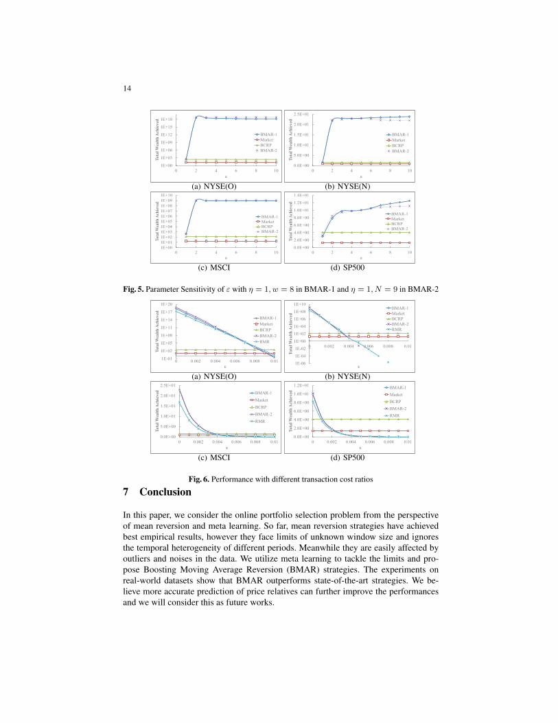
Impact of ε The passive-aggressive portfolio optimization technique is applied in ourscheme, which tends to keep the portfolios same unless they fail to reach the require-ment of return from each period. Therefore, we conduct experiments with differentvalues of ε to show the impact. The impact of ε on our strategies are similar. As shownin Fig. 5, both BMAR-1 and BMAR-2 achieve good performances on all datasets whenε ∈ [5, 10]. Similarly, we choose ε = 5 as a conventional setting.
6.5 Performance Under Transaction Costs
We also conduct experiments with different transaction cost ratio since it is an unavoid-able issue in practice. We alter the transaction cost ratio from 0% to 1% and computethe cumulative wealth of different strategies. The results are presented in Fig. 6.
Judging from the results, the transaction costs has a significant impact on the wealthreturn. When the transaction cost ratio is greater than 0.005, the wealth achieved onmost datasets is close to 0. Since our algorithms can still outperform the baselines, theyhave good scalability for transaction costs. Notice that the real transaction cost ratio isusually below 0.005, our algorithm can work well in practice.
14
1E+00
1E+03
1E+06
1E+09
1E+12
1E+15
1E+18
0 2 4 6 8 10
To
tal W
ea
lth
Ach
iev
ed
ε
BMAR-1
Market
BCRP
BMAR-2
(a) NYSE(O)
0.0E+00
5.0E+00
1.0E+01
1.5E+01
2.0E+01
2.5E+01
0 2 4 6 8 10
To
tal W
ea
lth
Ach
iev
ed
ε
BMAR-1
Market
BCRP
BMAR-2
(b) NYSE(N)
1E+00
1E+01
1E+02
1E+03
1E+04
1E+05
1E+06
1E+07
1E+08
1E+09
1E+10
0 2 4 6 8 10
To
tal
Wea
lth
Ach
iev
ed
ε
BMAR-1
Market
BCRP
BMAR-2
(c) MSCI
0.0E+00
2.0E+00
4.0E+00
6.0E+00
8.0E+00
1.0E+01
1.2E+01
1.4E+01
0 2 4 6 8 10
To
tal W
ea
lth
Ach
iev
ed
ε
BMAR-1
Market
BCRP
BMAR-2
(d) SP500
Fig. 5. Parameter Sensitivity of ε with η = 1, w = 8 in BMAR-1 and η = 1, N = 9 in BMAR-2
1E-01
1E+02
1E+05
1E+08
1E+11
1E+14
1E+17
1E+20
0 0.002 0.004 0.006 0.008 0.01
To
tal W
ea
lth
Ach
iev
ed
ε
BMAR-1
Market
BCRP
BMAR-2
RMR
(a) NYSE(O)
1E-06
1E-04
1E-02
1E+00
1E+02
1E+04
1E+06
1E+08
1E+10
0 0.002 0.004 0.006 0.008 0.01
To
tal W
ea
lth
Ach
iev
ed
ε
BMAR-1
Market
BCRP
BMAR-2
RMR
(b) NYSE(N)
0.0E+00
5.0E+00
1.0E+01
1.5E+01
2.0E+01
2.5E+01
0 0.002 0.004 0.006 0.008 0.01
To
tal W
ea
lth
Ach
iev
ed
ε
BMAR-1
Market
BCRP
BMAR-2
RMR
(c) MSCI
0.0E+00
2.0E+00
4.0E+00
6.0E+00
8.0E+00
1.0E+01
1.2E+01
0 0.002 0.004 0.006 0.008 0.01
To
tal W
ea
lth
Ach
iev
ed
ε
BMAR-1
Market
BCRP
BMAR-2
RMR
(d) SP500
Fig. 6. Performance with different transaction cost ratios
7 Conclusion
In this paper, we consider the online portfolio selection problem from the perspectiveof mean reversion and meta learning. So far, mean reversion strategies have achievedbest empirical results, however they face limits of unknown window size and ignoresthe temporal heterogeneity of different periods. Meanwhile they are easily affected byoutliers and noises in the data. We utilize meta learning to tackle the limits and pro-pose Boosting Moving Average Reversion (BMAR) strategies. The experiments onreal-world datasets show that BMAR outperforms state-of-the-art strategies. We be-lieve more accurate prediction of price relatives can further improve the performancesand we will consider this as future works.

15
8 Acknowledgement
This work was supported by the Natural Science Foundation (61532011, 61672311)of China and the National Key Basic Research Program (2015CB358700), part of thiswork was supported by the Center for Intelligent Information Retrieval.
References
1. Agarwal, A., Hazan, E., Kale, S., Schapire, R.E.: Algorithms for portfolio management basedon the newton method. pp. 9–16. ICML ’06, ACM, New York, NY, USA (2006)
2. Borodin, A., Elyaniv, R., Gogan, V.: Can we learn to beat the best stock. Journal of ArtificialIntelligence Research 21(1), 579–594 (2004)
3. Cesa-Bianchi, N., Lugosi, G.: Prediction, Learning, and Games. Cambridge University Press,New York, NY, USA (2006)
4. Cover, T.M., Thomas, J.A.: Elements of information theory. John Wiley & Sons (2012)5. Gaivoronski, A.A., Stella, F.: Stochastic nonstationary optimization for finding universal
portfolios. Annals of Operations Research 100(1), 165–188 (2000)6. Grinold, R., Kahn, R.: Active Portfolio Management: A Quantitative Approach for Producing
Superior Returns and Controlling Risk. McGraw-Hill Education (1999)7. Gyorfi, L., Lugosi, G., Udina, F.: Nonparametric kernel-based sequential investment strate-
gies. Mathematical Finance 16(2), 337–357 (2006)8. Helmbold, D.P., Schapire, R.E., Singer, Y., Warmuth, M.K.: On line portfolio selection using
multiplicative updates. Mathematical Finance 8(4), 325–347 (1998)9. Huang, D.J., Zhou, J., Li, B., Hoi, S., Zhou, S.: Robust median reversion strategy for online
portfolio selection. IEEE Transactions on Knowledge and Data Engineering 28(9), 2480–2493 (2016)
10. Kalai, A., Vempala, S.: Efficient algorithms for universal portfolios. Journal of MachineLearning Research 3(3), 423–440 (2003)
11. Kelly, J.L.: A new interpretation of information rate. Bell System Technical Journal 35(4),917–926 (1956)
12. Laszlo, G., Frederic, U., Harro, W.: Nonparametric nearest neighbor based empirical portfo-lio selection strategies. Statistics & Decisions 26(2), 145–157 (2008)
13. Li, B., Hoi, S.C.H.: Online portfolio selection: A survey. ACM Comput. Surv. 46(3), 1–36(Jan 2014)
14. Li, B., Hoi, S.C.H., Sahoo, D., Liu, Z.: Moving average reversion strategy for on-line port-folio selection. Artificial Intelligence 222, 104–123 (2015)
15. Li, B., Hoi, S.C.H., Zhao, P., Gopalkrishnan, V.: Confidence weighted mean reversion strat-egy for online portfolio selection. ACM Trans. Knowl. Discov. Data 7(1), 1–38 (Mar 2013)
16. Li, B., Hoi, S.C., Gopalkrishnan, V.: Corn: Correlation-driven nonparametric learning ap-proach for portfolio selection. ACM Trans. Intell. Syst. Technol. 2(3), 1–29 (May 2011)
17. Li, B., Zhao, P., Hoi, S.C.H., Gopalkrishnan, V.: Pamr: Passive aggressive mean reversionstrategy for portfolio selection. Machine Learning 87(2), 221–258 (2012)
18. Lo, A.W., Mackinlay, A.C.: When are contrarian profits due to stock market overreaction.Review of Financial Studies 3(2), 175–205 (1989)
19. MARKOWITZ, H.: Portfolio selection. The Journal of Finance 7, 1, 77C91 (1952)20. Merton, R.C.: On estimating the expected return on the market: An exploratory investigation.
Journal of Financial Economics 8(4), 323–361 (1980)21. Suykens, J.A.: Advances in learning theory: methods, models, and applications, vol. 190.
IOS Press (2003)