bootstrapping structure into language: alignment-based
TRANSCRIPT

arX
iv:c
s/02
0502
5v1
[cs.
LG]
16 M
ay 2
002
Bootstrapping Structure into Language:
Alignment-Based Learning
by
Menno M. van Zaanen
Submitted in accordance with the requirements
for the degree of Doctor of Philosophy.
The University of Leeds
School of Computing
September 2001
The candidate confirms that the work submitted is his own and the
appropriate credit has been given where reference has been made to the
work of others.

Abstract. . . refined and abstract meanings largely grow out of more concrete meanings.
— Bloomfield (1933)
This thesis introduces a new unsupervised learning framework, called Alignment-
Based Learning, which is based on the alignment of sentences and Harris’s (1951)
notion of substitutability. Instances of the framework can be applied to an untagged,
unstructured corpus of natural language sentences, resulting in a labelled, bracketed
version of that corpus.
Firstly, the framework aligns all sentences in the corpus in pairs, resulting in
a partition of the sentences consisting of parts of the sentences that are equal in
both sentences and parts that are unequal. Unequal parts of sentences can be seen
as being substitutable for each other, since substituting one unequal part for the
other results in another valid sentence. The unequal parts of the sentences are thus
considered to be possible (possibly overlapping) constituents, called hypotheses.
Secondly, the selection learning phase considers all hypotheses found by the
alignment learning phase and selects the best of these. The hypotheses are selected
based on the order in which they were found, or based on a probabilistic function.
The framework can be extended with a grammar extraction phase. This ex-
tended framework is called parseABL. Instead of returning a structured version of
the unstructured input corpus, like the ABL system, this system also returns a
stochastic context-free or tree substitution grammar.
Different instances of the framework have been tested on the English ATIS cor-
pus, the Dutch OVIS corpus and the Wall Street Journal corpus. One of the in-
teresting results, apart from the encouraging numerical results, is that all instances
can (and do) learn recursive structures.
i

Acknowledgements“Yacc” owes much to a most stimulating collection of users,
who have goaded me beyond my inclination,
and frequently beyond my ability in their endless search for ”one more feature”.
Their irritating unwillingness to learn how to do things my way
has usually led to my doing things their way;
most of the time, they have been right.
— Johnson (1979, p. 376)
There are many people who helped me (in many different ways) to start, continue
and finish this thesis and the research described in it. Rens Bod, my supervisor for
this project, has been of great help, revising my writing, solving problems when
I was stuck and giving me back my enthusiasm for the research when times were
difficult (even though he might not even have noticed doing it).
Especially in the beginning of this research I have had discussions with many
people, especially the DOP group, consisting of Arjen Poutsma and Lars Hoogweg
among others, but also Mila Groot, Rob Freeman, Alexander Clark, and Gerardo
Sierra (who pointed the Edit-Distance algorithm out to me) need mentioning.
People at three universities have allowed me to work there. First of all, the
University of Leeds, where Dan Black, Vincent Devin, and John Elliott made me
feel welcome every time. Eric Atwell, my advisor, was always interested in my
current research and could point out some interesting features and applications I
had never even thought about. At the faculty of Humanities at the University of
Amsterdam, Remko Scha initially showed me the use of Data-Oriented Parsing in
error correction (where it all started) and Khalil Sima’an helped me with his efficient
DOP parser. With Pieter Adriaans and Marco Vervoort (who generated the EMILE
results for me) from the faculty of Science I had many interesting discussions when
ii

comparing their EMILE system to ABL. People at the University of Groningen,
especially Wouter Jansen (who allowed me to use his workspace), Wilbert Heeringa,
Roberto Bolognesi (who both had to cope with me working in their room), and John
Nerbonne (who helped me with many things) made life a lot easier.
Whenever I needed programming help or computer power, I could ask Lo van den
Berg, while Kurt Brauchli (working at the department of Pathology at the University
of Basel) explained the ins and outs of DNA/RNA structures and Rogier Blokland
(University of Groningen) supplied me with the Hungarian example sentences.
In the final stage of the process, Yorick Wilks of the University of Sheffield
accepted the task of external examiner of this thesis. I would like to thank him for
his useful comments, suggestions, and discussions.
Finally, I would like to thank my parents, who supported me throughout my life
(including the years I have done this research) and Tanja Gaustad who helped me
with many fruitful discussions and allowed me to spend time on my research even
though it meant me spending less time with her.
I could not have done it without you all.
iii

DeclarationsHow do you think he does it?
I don’t know!
What makes him so good?
— The Who (Tommy, Pinball Wizard)
Parts of the work presented in this thesis have been published in the following
articles:
van Zaanen, 1999a
Bootstrapping structure using similarity. In Monachesi, P., editor, Compu-
tational Linguistics in the Netherlands 1999—Selected Papers from the Tenth
CLIN Meeting, pages 235–245, Utrecht, the Netherlands. Universteit Utrecht.
van Zaanen, 1999b
Error correction using DOP. In De Roeck, A., editor, Proceedings of the Second
UK Special Interest Group for Computational Linguistics (CLUK2) (Second
Issue), pages 1–12, Colchester, UK. University of Essex.
van Zaanen, 2000a
ABL: Alignment-Based Learning. In Proceedings of the 18th International
Conference on Computational Linguistics (COLING); Saarbrucken, Germany,
pages 961–967. Association for Computational Linguistics (ACL).
van Zaanen, 2000b
Bootstrapping syntax and recursion using Alignment-Based Learning. In
Langley, P., editor, Proceedings of the Seventeenth International Conference on
Machine Learning, pages 1063–1070, Stanford:CA, USA. Stanford University.
iv

van Zaanen, 2000c
Learning structure using alignment based learning. In Kilgarriff, A., Pearce,
D., and Tiberius, C., editors, Proceedings of the Third Annual Doctoral Re-
search Colloquium (CLUK), pages 75–82. Universities of Brighton and Sussex.
van Zaanen, 2001
Building treebanks using a grammar induction system. Technical Report
TR2001.06, University of Leeds, Leeds, UK.
van Zaanen and Adriaans, 2001a
Alignment-based learning versus EMILE: A comparison. In Proceedings of
the Belgian-Dutch Conference on Artificial Intelligence (BNAIC); Amsterdam,
the Netherlands. to be published.
van Zaanen and Adriaans, 2001b
Comparing two unsupervised grammar induction systems: Alignment-Based
Learning vs. EMILE. Technical Report TR2001.05, University of Leeds, Leeds,
UK.
van Zaanen, 2002
Alignment-based learning versus data-oriented parsing. In Bod, R., Sima’an,
K., and Scha, R., editors, Data Oriented Parsing. Center for Study of Lan-
guage and Information (CSLI) Publications, Stanford:CA, USA. to be pub-
lished.
v

ContentsIn which we take stock of where we are and where we are going,
this being a good thing to do before continuing.
— Russell and Norvig (1995, p. 842)
1 Introduction 3
2 Learning by Alignment 5
2.1 Goals . . . . . . . . . . . . . . . . . . . . . . . . . . . . . . . . . . . . . 5
2.1.1 Usefulness . . . . . . . . . . . . . . . . . . . . . . . . . . . . . . . . . . 6
2.1.2 Minimum of information . . . . . . . . . . . . . . . . . . . . . . . . . . 7
2.2 Finding constituents . . . . . . . . . . . . . . . . . . . . . . . . . . . . . 9
2.3 Multiple sentences . . . . . . . . . . . . . . . . . . . . . . . . . . . . . . 14
2.4 Removing overlapping constituents . . . . . . . . . . . . . . . . . . . . . 16
2.5 Problems with the approach . . . . . . . . . . . . . . . . . . . . . . . . . 16
2.5.1 Incorrectly removing overlapping constituents . . . . . . . . . . . . . . 17
2.5.2 Criticism on Harris’s notion of substitutability . . . . . . . . . . . . . . 18
2.5.2.1 Chomsky’s objections to substitutability . . . . . . . . . . . . . . . . 18
2.5.2.2 Pinker’s objections to substitutability . . . . . . . . . . . . . . . . . 19
3 The ABL Framework 22
3.1 Input . . . . . . . . . . . . . . . . . . . . . . . . . . . . . . . . . . . . . . 23
3.2 Alignment learning . . . . . . . . . . . . . . . . . . . . . . . . . . . . . . 24
3.2.1 Find the substitutable subsentences . . . . . . . . . . . . . . . . . . . . 27
3.2.2 Insert a hypothesis in the hypothesis space . . . . . . . . . . . . . . . . 28
3.2.3 Clustering . . . . . . . . . . . . . . . . . . . . . . . . . . . . . . . . . . 31
3.3 Selection learning . . . . . . . . . . . . . . . . . . . . . . . . . . . . . . . 32
vi

3.4 Grammar extraction . . . . . . . . . . . . . . . . . . . . . . . . . . . . . 33
3.4.1 Comparing grammars . . . . . . . . . . . . . . . . . . . . . . . . . . . 34
3.4.2 Improving selection learning . . . . . . . . . . . . . . . . . . . . . . . . 34
4 Instantiating the Phases 36
4.1 Alignment learning instantiations . . . . . . . . . . . . . . . . . . . . . . 36
4.1.1 Alignment learning with edit distance . . . . . . . . . . . . . . . . . . 37
4.1.1.1 The edit distance algorithm . . . . . . . . . . . . . . . . . . . . . . . 39
4.1.1.2 Default alignment learning . . . . . . . . . . . . . . . . . . . . . . . 41
4.1.1.3 Biased alignment learning . . . . . . . . . . . . . . . . . . . . . . . . 43
4.1.2 Alignment learning with all alignments . . . . . . . . . . . . . . . . . . 45
4.2 Selection learning instantiations . . . . . . . . . . . . . . . . . . . . . . . 46
4.2.1 Non-probabilistic selection learning . . . . . . . . . . . . . . . . . . . . 46
4.2.2 Probabilistic selection learning . . . . . . . . . . . . . . . . . . . . . . 48
4.2.2.1 The probability of a hypothesis . . . . . . . . . . . . . . . . . . . . . 48
4.2.2.2 The probability of a combination of hypotheses . . . . . . . . . . . . 50
4.3 Grammar extraction instantiations . . . . . . . . . . . . . . . . . . . . . 53
4.3.1 Extracting a stochastic context-free grammar . . . . . . . . . . . . . . 53
4.3.2 Extracting a stochastic tree substitution grammar . . . . . . . . . . . . 54
5 Empirical Results 57
5.1 Quantitative results . . . . . . . . . . . . . . . . . . . . . . . . . . . . . . 57
5.1.1 Different evaluation approaches . . . . . . . . . . . . . . . . . . . . . . 58
5.1.2 Test environment . . . . . . . . . . . . . . . . . . . . . . . . . . . . . . 62
5.1.2.1 Treebanks . . . . . . . . . . . . . . . . . . . . . . . . . . . . . . . . . 62
5.1.2.2 Metrics . . . . . . . . . . . . . . . . . . . . . . . . . . . . . . . . . . 64
5.1.2.3 Tested systems . . . . . . . . . . . . . . . . . . . . . . . . . . . . . . 66
5.1.3 Test results and evaluation . . . . . . . . . . . . . . . . . . . . . . . . 67
5.1.3.1 Alignment learning systems . . . . . . . . . . . . . . . . . . . . . . . 68
5.1.3.2 Selection learning systems . . . . . . . . . . . . . . . . . . . . . . . . 70
5.1.3.3 Results on the Wall Street Journal corpus . . . . . . . . . . . . . . . 72
5.1.3.4 parseABL systems . . . . . . . . . . . . . . . . . . . . . . . . . . . . 73
5.1.3.5 Learning curve . . . . . . . . . . . . . . . . . . . . . . . . . . . . . . 74
5.2 Qualitative results . . . . . . . . . . . . . . . . . . . . . . . . . . . . . . 75
5.2.1 Syntactic constructions . . . . . . . . . . . . . . . . . . . . . . . . . . . 76
5.2.2 Recursion . . . . . . . . . . . . . . . . . . . . . . . . . . . . . . . . . . 77
vii
6 ABL versus the World 80
6.1 Background . . . . . . . . . . . . . . . . . . . . . . . . . . . . . . . . . . 80
6.2 Bird’s-eye view over the world . . . . . . . . . . . . . . . . . . . . . . . . 82
6.2.1 Systems using complete information . . . . . . . . . . . . . . . . . . . 82
6.2.2 Systems using positive information . . . . . . . . . . . . . . . . . . . . 83
6.2.2.1 Supervised systems . . . . . . . . . . . . . . . . . . . . . . . . . . . . 83
6.2.2.2 Unsupervised systems . . . . . . . . . . . . . . . . . . . . . . . . . . 85
6.3 Zooming in on EMILE . . . . . . . . . . . . . . . . . . . . . . . . . . . . 89
6.3.1 Theoretical comparison . . . . . . . . . . . . . . . . . . . . . . . . . . 91
6.3.2 Numerical comparison . . . . . . . . . . . . . . . . . . . . . . . . . . . 92
6.4 ABL in relation to the other systems . . . . . . . . . . . . . . . . . . . . 93
6.5 Data-Oriented Parsing . . . . . . . . . . . . . . . . . . . . . . . . . . . . 95
6.5.1 Incorporating ABL in DOP . . . . . . . . . . . . . . . . . . . . . . . . 95
6.5.1.1 Bootstrapping a tree grammar . . . . . . . . . . . . . . . . . . . . . 96
6.5.1.2 Robustness of the parser . . . . . . . . . . . . . . . . . . . . . . . . . 97
6.5.2 Recursive definition . . . . . . . . . . . . . . . . . . . . . . . . . . . . 98
7 Future Work: Extending the Framework 99
7.1 Equal parts as hypotheses . . . . . . . . . . . . . . . . . . . . . . . . . . 99
7.2 Weakening exact match . . . . . . . . . . . . . . . . . . . . . . . . . . . 100
7.3 Dual level constituents . . . . . . . . . . . . . . . . . . . . . . . . . . . . 101
7.4 Alternative statistics in selection learning . . . . . . . . . . . . . . . . . . 103
7.4.1 Smoothing . . . . . . . . . . . . . . . . . . . . . . . . . . . . . . . . . 103
7.4.2 Selection learning through parsing . . . . . . . . . . . . . . . . . . . . 103
7.4.2.1 Selection learning with an SCFG . . . . . . . . . . . . . . . . . . . . 104
7.4.2.2 Selection learning with an STSG . . . . . . . . . . . . . . . . . . . . 105
7.5 ABL with Data-Oriented Translation . . . . . . . . . . . . . . . . . . . . 105
7.6 (Semi-)Supervised Alignment-Based Learning . . . . . . . . . . . . . . . 107
7.7 More corpora . . . . . . . . . . . . . . . . . . . . . . . . . . . . . . . . . 109
8 Conclusion 113
Bibliography 116
viii

List of FiguresOn two occasions I have been asked [by members of Parliament!],
‘Pray, Mr. Babbage, if you put into the machine wrong figures, will the right
answers come out?’
I am not able rightly to apprehend the kind of confusion of ideas that could
provoke such a question.
— Charles Babbage
2.1 Sentence-meaning pairs . . . . . . . . . . . . . . . . . . . . . . . . . . . . 7
2.2 Constituents induce compression . . . . . . . . . . . . . . . . . . . . . . 11
2.3 Grammar size based on equal and unequal parts . . . . . . . . . . . . . . 12
2.4 Unequal parts of sentences generated by same non-terminal . . . . . . . . 13
3.1 Overview of the ABL framework . . . . . . . . . . . . . . . . . . . . . . 23
3.2† Alignment learning . . . . . . . . . . . . . . . . . . . . . . . . . . . . . . 28
4.1 Example edit transcript and alignment . . . . . . . . . . . . . . . . . . . 38
4.2† Edit distance: building the matrix . . . . . . . . . . . . . . . . . . . . . 41
4.3† Edit distance: finding a trace . . . . . . . . . . . . . . . . . . . . . . . . 42
4.4 Example of a filled edit distance table . . . . . . . . . . . . . . . . . . . 43
4.5† Finding all possible alignments . . . . . . . . . . . . . . . . . . . . . . . 47
4.6 Extracting an SCFG from a tree structure . . . . . . . . . . . . . . . . . 54
4.7 Example elementary trees . . . . . . . . . . . . . . . . . . . . . . . . . . 55
5.1 Evaluating a structure induction system . . . . . . . . . . . . . . . . . . 62
5.2 Tested ABL and parseABL systems . . . . . . . . . . . . . . . . . . . . . 66
†Figures with a † symbol following their numbers are algorithms.
ix

5.3 Left and right branching trees . . . . . . . . . . . . . . . . . . . . . . . . 67
5.4 Learning curve on the ATIS corpus . . . . . . . . . . . . . . . . . . . . . 75
5.5 Learning curve on the OVIS corpus . . . . . . . . . . . . . . . . . . . . . 76
6.1 Ontology of learning systems . . . . . . . . . . . . . . . . . . . . . . . . 81
6.2 Example clustering expressions in EMILE . . . . . . . . . . . . . . . . . 89
6.3 Using ABL to bootstrap a tree grammar for DOP . . . . . . . . . . . . . 96
6.4 Using ABL to adjust the tree grammar . . . . . . . . . . . . . . . . . . . 97
7.1 Extracting an SCFG from a fuzzy tree . . . . . . . . . . . . . . . . . . . 105
7.2 Learning structure in sentence pairs . . . . . . . . . . . . . . . . . . . . . 106
7.3 Linked tree structures . . . . . . . . . . . . . . . . . . . . . . . . . . . . 107
7.4 Structure in RNA . . . . . . . . . . . . . . . . . . . . . . . . . . . . . . . 112
x

List of TablesAnd this is a table ma’am. What in essence it consists of is a horizontal rectilinear
plane surface maintained by four vertical columnar supports, which we call legs.
The tables in this laboratory, ma’am, are as advanced in design as one will find
anywhere in the world.
— Frayn (1965)
5.1 Results alignment learning on the ATIS and OVIS corpus . . . . . . . . . 69
5.2 Number of hypotheses after alignment learning . . . . . . . . . . . . . . 69
5.3 Results selection learning on the ATIS corpus . . . . . . . . . . . . . . . 70
5.4 Results selection learning on the OVIS corpus . . . . . . . . . . . . . . . 71
5.5 Results ABL on the WSJ corpus . . . . . . . . . . . . . . . . . . . . . . 73
5.6 Results parseABL on the ATIS corpus . . . . . . . . . . . . . . . . . . . 74
6.1 Results of EMILE and ABL . . . . . . . . . . . . . . . . . . . . . . . . . 93
xi

PrefaceThe White Rabbit put on his spectacles.
‘Where shall I begin, please your Majesty?’ he asked.
‘Begin at the beginning,’ the King said, very gravely,
‘and go on till you come to the end: then stop.’
— Carroll (1982, p. 109)
Some years ago, I had a meeting with Remko Scha at the University of Amsterdam.
He mentioned an interesting research topic where the Data-Oriented Parsing (DOP)
framework (Bod, 1995) was to be used in error correction. During the research for my
Master’s thesis at the Vrije Universiteit, I implemented an error correction system
based on DOP and incorporated it in a C compiler (van Zaanen, 1997).
When I was nearly done with writing my thesis, Rens Bod contacted me and
asked me if I would be interested in a PhD position at the University of Leeds, which
would possibly allow me to continue the research I was doing. A short while later,
I got accepted and the work, I have done there, has led to the thesis now lying in
front of you.
The original idea for the research described in this thesis was to transfer the
error correction system from the field of computer science back into computational
linguistics (where the DOP framework originally came from).
The main disadvantage of using such an error correcting system to correct errors
in natural language sentences, however, is that the underlying grammar should be
fixed beforehand; the errors are corrected according to the grammar. In practice,
with natural language, it is often the case that the grammar itself is incorrect or
incomplete and the sentence is correct.
The topic of the research shifted from building an error correction system to
building a grammar correction system. Taking things to extremes, the final system
1

should be able to bootstrap a grammar from scratch. I started wondering how
people are able to learn grammars and I wondered how I could get a computer to
do the same.1
The result of this process is described in the rest of this thesis.
1It must be absolutely clear that the system in no way claims to be cognitively modelling humanlanguage learning, even though some aspects may be cognitively plausible.
2
Chapter 1
IntroductionAre you ready for a new sensation?
— David Lee Roth (Eat ’em and smile)
The increase of computer storage and processing power has opened the way for
new, more resource intensive linguistic applications that used to be unreachable.
The trend in increase of resources also creates new uses for structured corpora or
treebanks. In the mean time, wider availability of treebanks will account for new
types of applications. These new applications can already be found in several fields,
for example:
• Natural language parsing (Allen, 1995; Bod, 1998; Charniak, 1997; Jurafsky
and Martin, 2000),
• Evaluation of natural language grammars (Black et al., 1991; Sampson, 2000),
• Machine translation (Poutsma, 2000b; Sadler and Vendelmans, 1990; Way,
1999),
• Investigating unknown scripts (Knight and Yamada, 1999).
Even though the applications rely heavily on the availability of treebanks, in
practice it is often hard to find one that is suitable for the specific task. The main
reason for this is that building treebanks is costly.
3

Chapter 1 4 Introduction
Language learning systems1 may help to solve the above mentioned problem.
These systems structure plain sentences (without the use of a grammar) or learn
grammars, which can then be used to parse sentences. Parsing indicates possible
structures or completely structures the corpus, making annotation less time and
expertise intensive and therefore less costly. Furthermore, language learning systems
can be reused on corpora in different domains.
Because of the many uses and advantages of a language learning system, one
might try to build such a system. Unsupervised learning of syntactic structure,
however, is one of the hardest problems in NLP. Although people are adept at
learning grammatical structure, it is difficult to model this process and therefore it
is hard to make a computer learn structure similarly to humans.
The goal of the algorithms described in this thesis is not to model the human
process of language learning, even though the idea originated from trying to model
human language acquisition. Instead, the algorithm should, given unstructured
sentences, find the best structure. This means that the algorithm should assign a
structure to sentences which is similar to the structure people would give to those
sentences, but not necessarily in the same way humans do this, nor in the same time
or space restrictions.
The rest of this thesis is subdivided as follows. First, in chapter 2, the underlying
ideas of the system are discussed, followed by a more formal description of the
framework in chapter 3. Next, chapter 4 introduces several possible instantiations
of the different phases of the system, and chapter 5 contains the results of the
instantiations on different corpora. Since at that point the entire system has been
described and evaluated, it is then compared against other systems in the field in
chapter 6. Possible extensions of the basic systems are described in chapter 7 and
finally, chapter 8 concludes this thesis.
1Language learning systems are sometimes called structure bootstrapping, grammar induction,or grammar learning systems. These names are used interchangeably throughout this thesis. How-ever, when the emphasis is on grammar learning, bootstrapping, or induction, the system shouldat least return a grammar as output, in contrast to language learning systems which only need tobuild a structured corpus.

Chapter 2
Learning by AlignmentThus, the fiction of interchangeability is inhumane and inherently wasteful.
— Stroustrup (1997, p. 716)
This chapter will informally describe step by step how one might build a system
that finds the syntactic structure of a sentence without knowing the grammar be-
forehand. First, the main goals are reviewed, followed by the description of a method
for finding constituents. The method is then extended to be used for multiple sen-
tences. This method, however, introduces ambiguities, which will be resolved in the
following section. Finally, some criticism on the applied methods will be discussed.
2.1 Goals
It is widely acknowledged that the principal goal in linguistics is to characterise the
set of sentence-meaning pairs. Considering that linguistics deals with production and
perception of language, using sentence-meaning pairs corresponds to converting from
sentence to meaning in perception and from meaning to sentence in the production
process.
It may be obvious that directly finding these sentence-meaning mappings is dif-
ficult. Taking the (syntactic) structure1 of the sentence into account simplifies this
process. A system that finds sentence to meaning mappings (i.e. in the percep-
tion process), first analyses the sentence, generating the structure of the sentence
as an intermediate. Using this structure, the meaning of the sentence is computed
(Montague, 1974).1In this thesis, “structure” and “syntactic structure” are used interchangeably.
5

Chapter 2 6 Learning by Alignment
In this thesis, the structure of a sentence is considered to be in the form of a
tree structure. This is not an arbitrary choice. Apart from the fact that trees are
rather uncontroversial in linguistics, it is also true in general that “complex entities
produced by any process of unplanned evolution, . . . , will have tree structuring as a
matter of statistical necessity” (Sampson, 1997). Another reason is that “hierarchies
have a property, . . . , that greatly simplifies their behaviour” (Simon, 1969), which
will be illustrated in section 2.2.
If the sentences conform to a language, described by a known grammar, several
techniques exist to generate the syntactic structure of these sentences (see for exam-
ple the (statistical) parsing techniques in (Allen, 1995; Charniak, 1993; Jurafsky and
Martin, 2000)). However, if the underlying grammar of the sentences is not known,
these techniques cannot be used, since they rely on knowledge of the grammar.
This thesis will describe a method that generates the syntactic structure of a
sentence when the underlying grammar of the language (or the set of possible gram-
mars2) is not known. This type of system is called a structure bootstrapping system.
Following the discussion on the goals of linguistics in general, let us now concen-
trate on the goals of a structure bootstrapping system. The system described here
is developed with two goals in mind: usefulness and minimum of information. Both
goals will be described next.
2.1.1 Usefulness
The first goal of a structure bootstrapping system is to find structure. However,
arbitrary, random, incomplete or incorrect structure is not very useful. The main
goal of the system is to find useful structure.
Remember that the goal in linguistics is to find sentence-meaning pairs, using
structure as an intermediate. Useful structure, therefore, should help us find these
pairs. As a (very simple) example how structure can help, consider figure 2.1. When
a sentence in the left column has the (partial) structure as shown in the middle
column, the meaning (shown in the right column)3 can be computed by combining
the meaning of the separate parts.4
2The empiricist/nativist distinction will be discussed in section 2.1.2.3In this example, the meaning of a sentence is represented in an overly simple type of predicate
logic, where words in small caps represent the meaning of the word in the regular font. For example,like is the meaning of the word likes.
4How the transition from structure to meaning is found is outside the scope of this thesis. Itwill simply be assumed that such a transition is possible.

Chapter 2 7 Learning by Alignment
Based on the principle of compositionality of meaning (Frege, 1879), the mean-
ing of a sentence can be computed by combining the meaning of its constituents. In
general, the constituent on position X may be more than one word. If, for example,
the old man is found on position X, then the meaning of the sentence would be
likes(oscar, the old man). Of course, this example is too simple to be practi-
cal, but it illustrates how structured sentences can help in finding the meaning of
sentences.
Figure 2.1 Sentence-meaning pairs
Sentence ⇒ Structure ⇒ Meaning
Oscar likes trash ⇒ Oscar likes [trash] ⇒ like(oscar, trash)Oscar likes biscuits ⇒ Oscar likes [biscuits] ⇒ like(oscar, biscuits)Oscar likes X ⇒ Oscar likes [X ] ⇒ like(oscar, X )
Usefulness can be tested based on a predefined, manually structured corpus,
such as the Penn Treebank (Marcus et al., 1993), or the Susanne Corpus (Sampson,
1995). The structures of the sentences in such a corpus are considered completely
correct (i.e. each tree corresponds to the structure as it was perceived for the partic-
ular sentence uttered in a certain context). The structure learned by the structure
bootstrapping system is then compared against this true structure. First, plain sen-
tences are extracted from a given structured corpus. These plain sentences are the
input of the structure bootstrapping system. The output (structured sentences) can
be compared to the structured sentences of the original corpus and the complete-
ness (recall) and correctness (precision) of the learned structure can be computed.
Details of this evaluation method can be found in section 5.1.2.2.
2.1.2 Minimum of information
Structure bootstrapping systems can be grouped (like other learning methods) into
supervised and unsupervised systems. Supervised methods are initialised with struc-
tured sentences, while unsupervised methods only get to see plain sentences. In prac-
tice, supervised methods outperform unsupervised methods, since they can adapt
their output based on the structured examples in the initialisation phase whereas
unsupervised methods cannot.
Even though in general the performance of unsupervised methods is less than
that of supervised methods, it is worthwhile to investigate unsupervised grammar

Chapter 2 8 Learning by Alignment
learning methods. Supervised methods need structured sentences to initialise, but
“the costs of annotation are prohibitively time and expertise intensive, and the
resulting corpora may be too susceptible to restriction to a particular domain, ap-
plication, or genre” (Kehler and Stolcke, 1999a). Thus annotated corpora may not
always be available for a language. In contrast, unsupervised methods do not need
these structured sentences.
The second goal of the bootstrapping system can be described as learning using
a minimum of information. The system should try to minimise the amount of infor-
mation it needs to learn structure. Supervised systems receive structured examples,
which contain more information than their unstructured counterparts, so the second
goal restricts the system described in this thesis from being supervised.
In general, unsupervised systems may still use additional information. This ad-
ditional information may be for example in the form of a lexicon, part-of-speech tags
(Klein and Manning, 2001; Pereira and Schabes, 1992), many adjustable language
dependent settings in the system (Adriaans, 1992; Vervoort, 2000) or a combination
of language dependent information sources (Osborne, 1994).
However, since the goal of the system described here is to use a minimum of
information, the system must refrain from using extra information. The only lan-
guage dependent information the system may use is a corpus of plain sentences (for
example in the form of transcribed acoustic utterances). Using this information it
outputs the same corpus augmented with structure (or a compact representation of
this structure, for example in the form of a grammar).
The advantages of using a minimum of information are legion. Since no language
specific knowledge is needed, it can be used on languages for which no structured
corpora or dictionaries exist. It can even be used on unknown languages. Fur-
thermore, it does not need extensive tuning (since the system does not have many
adjustable settings).
By assuming the goal of minimum of information, the learning method should
be classified as an empiricist approach. According to Chomsky (1965, pp. 47–48):
The empiricist approach has assumed that the structure of the acquisi-
tion device is limited to certain elementary “peripheral processing mech-
anisms”. . . Beyond this, it assumes that the device has certain analytical
data-processing mechanisms or inductive principles of a very elementary
sort, . . .

Chapter 2 9 Learning by Alignment
In contrast to the empiricist approach, there is the nativist (or rationalist) ap-
proach:
The rationalist approach holds that beyond the peripheral processing
mechanisms, there are innate ideas and principles of various kinds that
determine the form of the acquired knowledge in what may be a rather
restricted and highly organised way.
The nativist approach assumes innate ideas and principles (for example an in-
nate universal grammar describing all possible languages). The empiricist approach,
however, is more closely linked to the idea of minimum of information.
Note that instead of refuting the nativist approach, the work described in this
thesis is an attempt to show how much can be learned using an empiricist approach.
Now that the goals of the system are set, a first attempt will be made to meet
these goals. The rest of the chapter develops a method that adheres to the first goal
(usefulness), while keeping the second goal in mind.
2.2 Finding constituents
Starting with the first goal of the system, usefulness, constituents need to be found
in unstructured text. To get an idea of the exact problem, imagine seeing text in
an unknown language (unknown to you). How would you try to find out which
words belong to the same syntactic type (for example, nouns) or which words group
together to form, for example, a noun phrase? (Remember that the goal is not to
find a model of human language learning. However, thinking about how one searches
for structure might also help in finding a way to automatically structure text.)
Let us start with the simplest case. If you see one sentence in an unknown
language then what can you conclude from that? (Try for example sentence 1a.) If
you do not know anything about the language, it is very hard if not impossible5 to
say anything about the structure of the sentence (but you can conclude that it is a
sentence).
However, if two sentences are available, it is possible to find parts of the sentences
that are the same in both and parts that are not (provided that some words are
the same and some words are different in both sentences). The comparison of two
sentences falls into one of three different categories:
5Using for example universal rules or expected distributions of word classes, it may be possibleto find some structure in one plain sentence.

Chapter 2 10 Learning by Alignment
1. All words in the two sentences are the same (and so is the order of the words).6
2. The sentences are completely unequal (i.e. there is not one word that can be
found in both sentences).
3. Some words in the sentences are the same in both and some are not.
It may be clear that the third case is the most interesting one. The first case
does not yield any additional information. It was already known that the sentence
was a sentence. No new knowledge can be induced from seeing it another time. The
second case illustrates that there are more sentences, but since there is no relation
between the two, it is impossible to extract any further useful information.
The sentences contained in the third case give more information. They show
different contexts of the same words. These different contexts of the words might
help find structure in the two sentences.
Let us now consider the pairs of sentences in 1 and 2. It is possible to group
words that are equal and words that are unequal in both sentences. The word groups
that are equal in both sentences are underlined.
(1) a. Bert sut egy kekszet
b. Ernie eszi a kekszet
(2) a. Bert sut egy kekszet
b. Bert sut egy kalacsot
These sentences are simple cases of the more complex sentences where there are
more groups of equal and unequal words. The more complex examples can be seen
as concatenations of the simple cases. Therefore, these simple sentences can be used
without loss of generality.
Although it is clear which words are the same in both sentences (and which are
not), it is still unclear which parts are constituents. The Hungarian sentences in 1
translate to the English sentences as shown in 3.7 In this case, it is clear that the
6Previous publications mentioned “similar” and “dissimilar” instead of “equal” and “unequal”in this context. However, apart from section 7.2 where the exact match is weakened, sentences areonly considered equal if the words in the two sentences are exactly the same (and not just similar).
7For the sake of the argument, we may assume that the word order of the two languages is thesame, but this need not necessarily be so, i.e. our argument does not depend on this (languagedependent) assumption.

Chapter 2 11 Learning by Alignment
underlined word groups (consisting of one word) should be constituents.8 Biscuit is
a constituent, but Bert is baking a and Ernie is eating the are not.
(3) a. Bert sut egy [kekszet]X1
Bert-nom-sg to bake-pres-3p-sg-indef a-indef biscuit-acc-sg
Bert is baking a [biscuit]X1
b. Ernie eszi a [kekszet]X1
Ernie-nom-sg to eat-pres-3p-sg-def the-def biscuit-acc-sg
Ernie is eating the [biscuit]X1
However, if we conclude that equal parts in sentences are always constituents,
the sentences in 2 will be structured incorrectly. These sentences are translated as
shown in 4. In this case, the unequal parts of the sentences are constituents. Biscuit
and cake are constituents, but Bert is baking a is not.
(4) a. Bert sut egy [kekszet]X2
Bert-nom-sg to bake-pres-3p-sg-indef a-indef biscuit-acc-sg
Bert is baking a [biscuit]X2
b. Bert sut egy [kalacsot]X2
Bert-nom-sg to bake-pres-3p-sg-indef a-indef cake-acc-sg
Bert is baking a [cake]X2
Intuitively, choosing constituents by treating unequal parts of sentences as con-
stituents (as shown in the sentences of 4) is preferred over constituents of equal parts
of sentences (as indicated by the sentences in 3). This will be shown (in two ways)
by considering the underlying grammar.
Figure 2.2 Constituents induce compression
Method Structure Grammar
Equal parts [[Bert sut egy]X kekszet]S S→X kekszet[[Bert sut egy]X kalacsot]S S→X kalacsot
X→Bert sut egyUnequal parts [Bert sut egy [kekszet]X]S S→Bert sut egy X
[Bert sut egy [kalacsot]X]S X→kekszetX→kalacsot
8X1 and X2 denote non-terminal types.

Chapter 2 12 Learning by Alignment
The main argument for choosing unequal parts of sentences instead of equal
parts of sentences as constituents is that the resulting grammar is smaller. When
unequal parts of sentences are taken to be constituents, this results in more compact
grammars than when equal parts of sentences are taken to be constituents. In other
words, the grammar is more compressed.
An example of the stronger compression power of the unequal parts of sentences
can be found in figure 2.2. If the length of a grammar is defined as the number of
symbols in the grammar, then the length of the first grammar is 10. However, the
length of the second grammar is 9.
In general, it is the case that making constituents of unequal parts of sentences
creates a smaller grammar. Imagine aligning two sentences (and, to keep things
simple, assume there is one equal part and one unequal part in both sentences).
The equal parts of the two sentences is defined as E and the unequal part of the
first sentence is U1 and of the second sentence U2.
Figure 2.3 Grammar size based on equal and unequal parts
Method Grammar Size
Equal parts S→X U1 1 + 1 + |U1|S→X U2 1 + 1 + |U2|X→E 1 + |E|total 5 + |U1|+ |U2|+ |E|
Unequal parts S→E X 1 + |E|+ 1X→U1 1 + |U1|X→U2 1 + |U2|total 4 + |U1|+ |U2|+ |E|
Figure 2.3 shows that taking unequal parts of sentences as constituents create
slightly smaller grammars.9 In the rightmost column, the grammar size is computed.
Each non-terminal counts as 1 and the sizes of the equal and unequal parts are also
incorporated.
For the second argument, assume the sentences are generated from a context-free
grammar. This means that for each of the two sentences there is a derivation that
leads to that sentence. Figure 2.4 shows the derivations of two sentences, where a
and b are the unequal parts of the sentences (the rest is the same in both). The idea
is now that the unequal parts of the sentences are both generated from the same
9The order of the non-terminals and the sentence parts may vary. This does not change theresulting grammar size.

Chapter 2 13 Learning by Alignment
Figure 2.4 Unequal parts of sentences generated by same non-terminal
S
X
a
S
X
b
non-terminal, which would indicate that they are constituents of the same type.
Note that this is not necessarily the case, as is shown in the example sentences in 3.
However, changing one of the sentences in 3 to the other one, would require several
non-terminals to have different yields10, whereas taking unequal parts of sentences
as constituents means that only one non-terminal needs to have a different yield.
These two arguments indicate a preference for the method that takes unequal
parts of sentences as constituents. Additionally, the idea closely resembles the lin-
guistically motivated and language independent notion of substitutability. Harris
(1951, p. 30) describes freely substitutable segments as follows:
If segments are freely substitutable for each other they are descriptively
equivalent, in that everything we henceforth say about one of them will
be equally applicable to the others.
Harris continues by describing how substitutable segments can be found:
We take an utterance whose segments are recorded as DEF. We now
construct an utterance composed of the segments DA’F, where A’ is a
repetition of a segment A in an utterance which we had represented as
ABC. If our informant accepts DA’F as a repetition of DEF, or if we
hear an informant say DA’F, and if we are similarly able to obtain E’BC
(E’ being a repetition of E) as equivalent to ABC, then we say that A
and E (and A’ and E’) are mutually substitutable (or equivalent), as
free variants of each other, and write A=E. If we fail in these tests, we
say that A is different from E and not substitutable for it.
When Harris’s test is simplified or reduced (removing the need for repetitions),
the following test remains: “If the occurrences DEF, DAF, ABC and EBC are
found, A and E are substitutable.”
10If changing the sentences would only require one non-terminal to be changed, the situation infigure 2.4 arises again.
Chapter 2 14 Learning by Alignment
The simplified test is instantiated with constituents as segments.11 We conclude
that if constituents are found in the same context, they are substitutable and thus of
the same type. This is equivalent to finding constituents as is shown in the sentences
in 4.
The test for finding constituents is intuitively assumed correct (however, see
section 2.5.2 for criticism of this approach). A constituent of a certain type can
be replaced by another constituent of the same type, while still retaining a valid
sentence. Therefore, if two sentences are the same except for a certain part, it
might be the case that these two sentences were generated by replacing a certain
constituent by another one of the same type.
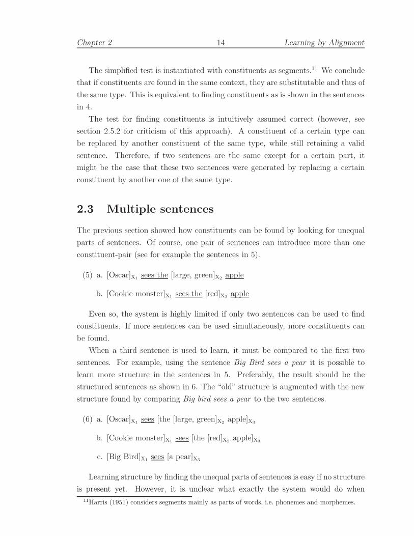
2.3 Multiple sentences
The previous section showed how constituents can be found by looking for unequal
parts of sentences. Of course, one pair of sentences can introduce more than one
constituent-pair (see for example the sentences in 5).
(5) a. [Oscar]X1sees the [large, green]X2
apple
b. [Cookie monster]X1sees the [red]X2
apple
Even so, the system is highly limited if only two sentences can be used to find
constituents. If more sentences can be used simultaneously, more constituents can
be found.
When a third sentence is used to learn, it must be compared to the first two
sentences. For example, using the sentence Big Bird sees a pear it is possible to
learn more structure in the sentences in 5. Preferably, the result should be the
structured sentences as shown in 6. The “old” structure is augmented with the new
structure found by comparing Big bird sees a pear to the two sentences.
(6) a. [Oscar]X1sees [the [large, green]X2
apple]X3
b. [Cookie monster]X1sees [the [red]X2
apple]X3
c. [Big Bird]X1sees [a pear]X3
Learning structure by finding the unequal parts of sentences is easy if no structure
is present yet. However, it is unclear what exactly the system would do when
11Harris (1951) considers segments mainly as parts of words, i.e. phonemes and morphemes.
Chapter 2 15 Learning by Alignment
some constituents are already present in the sentence. The easiest way of handling
this is to compare the plain sentences (temporarily forgetting any structure already
present). When some structure is found it is then added to the already existing
structure.
In example 6, sentences 6a and 6b are compared first (as shown in 5). The
plain sentence 6c is then compared against the plain sentence of 6a. This adds the
constituents with type X3 to sentences 6a and 6c and the constituent of type X1 to
sentence 6c.
Sentence 6c then already has the structure as shown. However, it is still compared
against sentence 6b, since some more structure might be induced. Indeed, when
comparing the plain sentences 6b and 6c, sentence 6b also receives the constituents
with types X3.
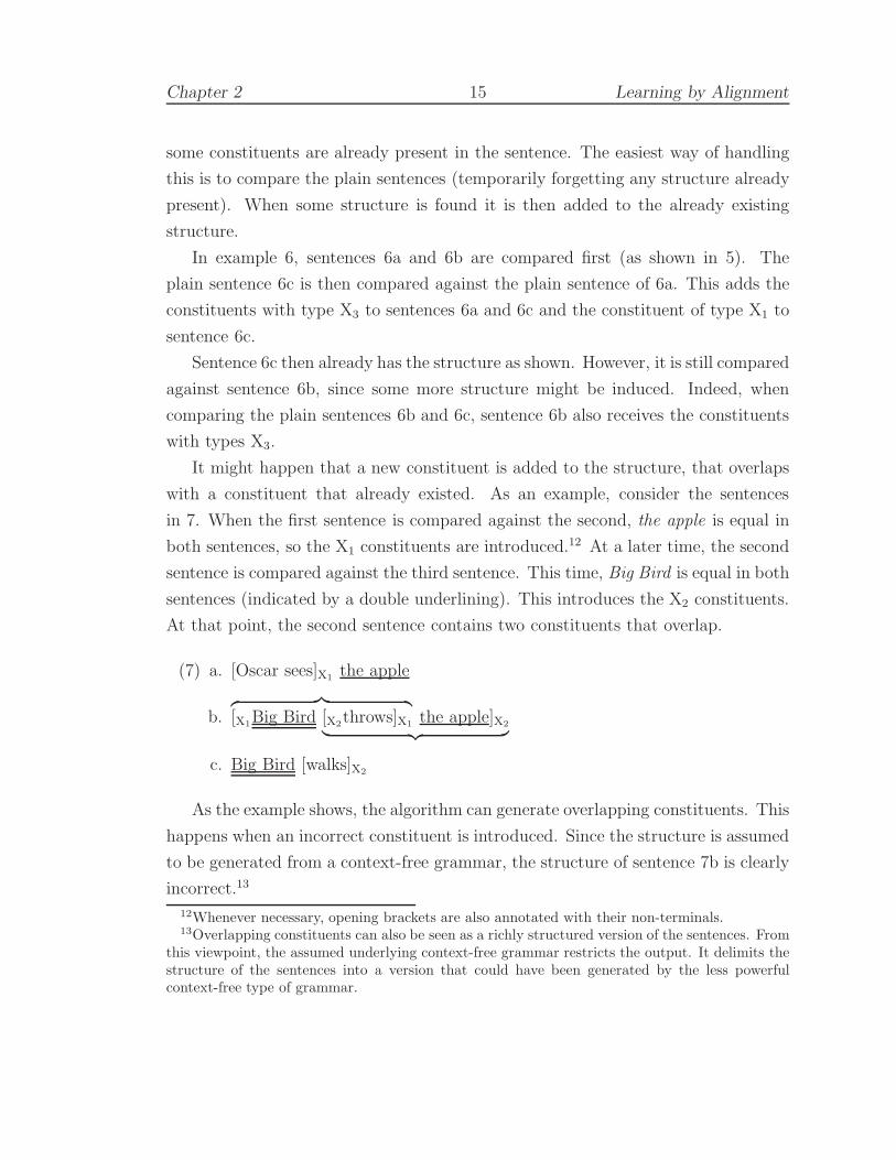
It might happen that a new constituent is added to the structure, that overlaps
with a constituent that already existed. As an example, consider the sentences
in 7. When the first sentence is compared against the second, the apple is equal in
both sentences, so the X1 constituents are introduced.12 At a later time, the second
sentence is compared against the third sentence. This time, Big Bird is equal in both
sentences (indicated by a double underlining). This introduces the X2 constituents.
At that point, the second sentence contains two constituents that overlap.
(7) a. [Oscar sees]X1the apple
b.︷ ︸︸ ︷
[X1Big Bird
︸ ︷︷ ︸[X2
throws]X1the apple]X2
c. Big Bird [walks]X2
As the example shows, the algorithm can generate overlapping constituents. This
happens when an incorrect constituent is introduced. Since the structure is assumed
to be generated from a context-free grammar, the structure of sentence 7b is clearly
incorrect.13
12Whenever necessary, opening brackets are also annotated with their non-terminals.13Overlapping constituents can also be seen as a richly structured version of the sentences. From
this viewpoint, the assumed underlying context-free grammar restricts the output. It delimits thestructure of the sentences into a version that could have been generated by the less powerfulcontext-free type of grammar.

Chapter 2 16 Learning by Alignment
2.4 Removing overlapping constituents
If the system is trying to learn structure that can be generated by a context-free
(or mildly context-sensitive) grammar, overlaps should never occur within one tree
structure. However, the system so far can (and does) introduce overlapping con-
stituents.
Assuming that the underlying grammar is context-free is not an arbitrary choice.
To evaluate learning systems (amongst others), a structured corpus is taken to
compute the recall and precision. Most structured corpora are built on a context-
free (or weakly context-sensitive) grammar and thus do not contain overlapping
constituents within a sentence.
The system described so far needs to be modified so that the final structured
sentences do not have overlapping constituents. This will be the second phase in
the system. There are many different, possible ways of accomplishing this, but as
a first instantiation, the system will make the (very) simple assumption that con-
stituents learned earlier are always correct.14 This means that when a constituent is
introduced that overlaps with an already existing constituent, the newer constituent
is considered incorrect. If this happens, the new constituent is not introduced into
the structure. This will make sure that no overlapping constituents are stored.
Other instantiations, based on a probabilistic evaluation method, will be explained
in chapter 4.
The next section will describe overall problems of the method described so far
(including the problems of this approach of solving overlapping constituents). Im-
proved methods that remove overlapping constituents will be discussed in section 4.2
on page 46.
2.5 Problems with the approach
There seem to be two problems with the structure bootstrapping approach as de-
scribed so far. First, removing overlapping constituents as described in the previous
section, although solving the problem, is clearly incorrect. Second, the underlying
idea of the method, Harris’s notion of substitutability, has been heavily criticised.
Both problems will be described in some detail next.
14It must be completely clear that assuming that older constituents are correct is not a featureof the general framework (which will be described in the next chapter), but merely a particularinstantiation of this phase.

Chapter 2 17 Learning by Alignment
2.5.1 Incorrectly removing overlapping constituents
The method of finding constituents as described in section 2.2 on page 9 may, at some
point, find overlapping constituents. Since overlapping constituents are unwanted,
as discussed above, the system takes the older constituents as correct, removing the
newer constituents.
Even though there is evidence that “analyses that a person has experienced
before are preferred to analyses that must be newly constructed” (Bod, 1998, p. 3),
it is clear that applying this idea directly will generate incorrect results. It is easily
imagined that when the order of the sentences is different, the final results will be
different, since different constituents are seen earlier.
Let us reflect on why exactly constituents are removed. If overlapping con-
stituents are unwanted, then clearly the method of finding constituents, which in-
troduces these overlapping constituents, is incorrect.
Before discarding the work done so far, it may be helpful to reconsider the used
terminology. Another way of looking at the approach is to say that the method which
finds constituents does not really introduce constituents, but instead it introduces
hypotheses about constituents.
“Finding constituents” really builds a hypothesis space, where possible con-
stituents in the sentences are stored. “Removing overlapping constituents” searches
this hypothesis space, removing hypotheses until the best remain.
Clearly, a better system would keep (i.e. not remove) hypotheses if there is more
evidence for them. In this case, evidence can be defined in terms of frequency. Hy-
potheses that have a higher frequency are more likely to be correct. Older hypotheses
can now be overruled by newer hypotheses if the latter have a higher frequency. Sec-
tion 4.2 on page 46 contains two hypothesis selection methods based on this idea.
Using probabilities to select hypotheses makes the system described in this thesis
a Bayesian learning method. The goal is to maximise the probability of a set of
(non-overlapping) hypotheses for a sentence given that sentence.
Selecting constituents based on their frequency is an intuitively correct solution.
But, apart from that, the notion of selecting structure based on frequencies is un-
controversial in psychology. “More frequent analyses are preferred to less frequent
ones” (Bod, 1998, p. 3).

Chapter 2 18 Learning by Alignment
2.5.2 Criticism on Harris’s notion of substitutability
Harris’s notion of substitutability has been heavily criticised. However, most criti-
cism is similar in nature to: “. . . , although there is frequent reference in the litera-
ture of linguistics, psychology, and philosophy of language to inductive procedures,
methods of abstraction, analogy and analogical synthesis, generalisation, and the
like, the fundamental inadequacy of these suggestions is obscured only by their
unclarity”(Chomsky, 1955, p. 31) or “Structuralist theories, both in the European
and American traditions, did concern themselves with analytic procedures for deriv-
ing aspects of grammar from data, as in the procedural theories of . . . Zellig Harris,
. . . primarily in the areas of phonology and morphology. The procedures suggested
were seriously inadequate . . . ”(Chomsky, 1986, p. 7). There are only a few places
where Harris’s notion of substitutability is really questioned. See (Redington et al.,
1998) for a discussion of the problems described in (Pinker, 1984).
The next two sections will discuss serious objections by Chomsky and Pinker
respectively.
2.5.2.1 Chomsky’s objections to substitutability
Chomsky (1955, pp. 129–145) gives a nice overview of problems when the notion of
substitutability is used. In his argumentation, he introduces four problems. Three
of these problems are relevant to the system described in this thesis, so these will
be discussed in some detail.15
Chomsky describes the first problem as:
In any sample of linguistic material, no two words can be expected to
have exactly the same set of contexts. On the other hand, many words
which should be in different contexts will have some context in common.
. . . Thus substitution is either too narrow, if we require complete mutual
substitutability for co-membership in a syntactic category . . . , or too
broad, if we require only that some context be shared.
The structure bootstrapping system uses the “broad” method for substitutability.
Hypotheses are introduced when “some context” is shared. This will introduce too
many hypotheses and some of the introduced hypotheses might have an incorrect
type (as Chomsky rightly points out). However, when overlapping hypotheses are
removed, the more likely hypotheses will remain.
15The fourth problem deals with a measure of grammaticality of sentences.

Chapter 2 19 Learning by Alignment
So far, Chomsky talked about substitutability of words. In the second problem
he states: “We cannot freely allow substitution of word sequences for one another.”
According to Chomsky, this cannot be done, since it will introduce incorrect con-
stituents.
The solution to this problem is similar to the solution of the first problem. Since
hypotheses about constituents are stored and afterwards the best hypotheses are
selected, we conjecture that probably no incorrect constituents will be contained in
the final structure. This conjecture will be tested extensively in chapter 5.
Chomsky’s last problem deals with homonyms: “[Homonyms] are best under-
stood as belonging simultaneously to several categories of the same order.” Pinker
discussed this problem extensively. His discussion will be dealt with next.
2.5.2.2 Pinker’s objections to substitutability
Pinker (1994, pp. 283–288) discusses two problems that deal with the notion of
substitutability. The first problem deals with words that receive an incorrect type.
For the second problem, Pinker shows that finding one-word constituents is not
enough. Instead of classifying words, phrases need to be classified. He then shows
that there are too many ways of doing this, concluding that the problem is too
difficult to solve in an unsupervised way.
When describing the first problem, Pinker shows how structure can be learned
by considering the sentences in 8.
(8) a. Jane eats chicken
b. Jane eats fish
c. Jane likes fish
From this, he concludes that sentences contain three words, Jane, followed by eats
or likes, again followed by chicken or fish. This is exactly what the structure boot-
strapping system described in this thesis does. He then continues by giving the
sentences as in 9.
(9) a. Jane eats slowly
b. Jane might fish
However, this introduces inconsistencies, since might may now appear in the second
position and slowly may appear in the third position, rendering sentences like Jane
might slowly, Jane likes slowly and Jane might chicken correct.

Chapter 2 20 Learning by Alignment
This is a complex problem and the current system, which selects hypotheses
based on the chronological order of learning hypotheses, cannot cope with it. How-
ever, a probabilistic system (that assigns types to hypotheses based on probabilities)
will be able to solve this problem. In section 7.3 on page 101 a solution to this prob-
lem is discussed in more detail, but the main line of the solution is briefly described
here.
The problem with Pinker’s approach (and actually Harris makes the same mis-
take) is that he does not allow his system to recognise that words may belong to
different classes. In other words, his approach will assign one class to a word (or in
general, a phrase), for example a word is a noun and nothing else. This is clearly
incorrect, as can be seen in sentences 8b and 8c (fish is a noun) and sentence 9b
(fish is a verb).
However, the contexts of a word that does not have one clear type help to
distinguish between the different types. A noun like fish can occur in places in
sentences where the verb fish cannot. Consider for example the sentences in 10.
The noun fish can never occur in the context of the first sentence, while the verb
fish cannot occur in the context of the second sentence.
(10) a. We fish for trout
b. Jane eats fish
Using these differences in contexts, a word may be classified as having a certain
type in one context and another type in another context. For example, verb-like
words occur in verb contexts and noun-like words occur in noun contexts. The
frequencies of the word in the different contexts indicate which type the word has
in a specific context.
Pinker continues with the second problem. He wonders what word could occur
before the word bother when he shows the sentences in 11. This introduces a prob-
lem, since there are many different types of words that may occur before bother.
From this, he concludes that looking for a phrase is the solution (a noun phrase in
this particular case).
(11) a. That dog bothers me [dog, a noun]
b. What she wears bothers me [wears, a verb]
c. Music that is too loud bothers me [loud, an adjective]
d. Cheering too loudly bothers me [loudly, an adverb]

Chapter 2 21 Learning by Alignment
e. The guy she hangs out with bothers me [with, a preposition]
Pinker then suggests considering all possible ways to group words into phrases.
This results in 2n−1 possibilities if the sentence has length n. Since there are too
many possibilities, the child (in our case, the structure bootstrapping system) needs
additional guidance. This additional guidance clashes with the goal of minimum
of information, so Pinker implies that an unsupervised bootstrapping system is not
feasible.
We believe that Pinker missed the point here. It is clear that applying the system
that has been described earlier in this chapter to the sentences in 11 will find exactly
the correct constituents. In all sentences the words before bothers me are grouped
in constituents of the same type. In other words, the system does not need any
guiding as Pinker wants us to believe.

Chapter 3
The ABL FrameworkOne or two homologous sequences whisper . . .
a full multiple alignment shouts out loud.
— Hubbard et al. (1996)
The structure bootstrapping system described informally in the previous chapter
is one of many possible instances of a more general framework. This framework is
called Alignment-Based Learning (ABL) and will be described more formally in this
chapter.
Specific instances of ABL attempt to find structure using a corpus of plain (un-
structured) sentences. They do not assume a structured training set to initialise,
nor are they based on any other language dependent information. All structural
information is gathered from the unstructured sentences only. The output of the
algorithm is a labelled, bracketed version of the input corpus. This corresponds to
the goals as described in section 2.1.
The ABL framework consists of two distinct phases:
1. alignment learning
2. selection learning
The alignment learning phase is the most important, in that it finds hypotheses
about constituents by aligning sentences from the corpus. The selection learning
phase selects constituents from the possibly overlapping hypotheses that are found
by the alignment learning phase.
22
Chapter 3 23 The ABL Framework
Although the ABL framework consists of these two phases, it is possible (and
useful) to extend this framework with another phase:
3. grammar extraction
As the name suggests, this phase extracts a grammar from the structured corpus
(as created by the alignment and selection learning phases). This extended system
is called parseABL.1
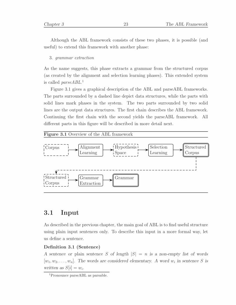
Figure 3.1 gives a graphical description of the ABL and parseABL frameworks.
The parts surrounded by a dashed line depict data structures, while the parts with
solid lines mark phases in the system. The two parts surrounded by two solid
lines are the output data structures. The first chain describes the ABL framework.
Continuing the first chain with the second yields the parseABL framework. All
different parts in this figure will be described in more detail next.
Figure 3.1 Overview of the ABL framework
Corpus AlignmentLearning
HypothesisSpace
SelectionLearning
StructuredCorpus
StructuredCorpus
GrammarExtraction
Grammar
3.1 Input
As described in the previous chapter, the main goal of ABL is to find useful structure
using plain input sentences only. To describe this input in a more formal way, let
us define a sentence.
Definition 3.1 (Sentence)
A sentence or plain sentence S of length |S| = n is a non-empty list of words
[w1, w2, . . . , wn]. The words are considered elementary. A word wi in sentence S is
written as S[i] = wi.
1Pronounce parseABL as parsable.

Chapter 3 24 The ABL Framework
ABL cannot learn using only one sentence, it uses more sentences to find struc-
ture. The sentences it uses are stored in a list called a corpus. Note that according
to the definition, a corpus can never contain structured sentences.
Definition 3.2 (Corpus)
A corpus U of size |U | = n is a list of sentences [S1, S2, . . . Sn].
3.2 Alignment learning
A corpus of sentences is used as (unstructured) input. The framework attempts to
find structure in this corpus. The basic unit of structure is a constituent, which
describes a group of words.
Definition 3.3 (Constituent)
A constituent in sentence S is a tuple cS = 〈b, e, n〉 where 0 ≤ b ≤ e ≤ |S|. b and e
are indices in S denoting respectively the beginning and end of the constituent. n
is the non-terminal of the constituent and is taken from the set of non-terminals. S
may be omitted when its value is clear from the context.
The goal of the ABL framework is to introduce constituents in the unstructured
input sentences. The alignment learning phase indicates where in the input sen-
tences constituents may occur. Instead of introducing constituents, the alignment
learning phase indicates possible constituents. These possible constituents are called
hypotheses.
Definition 3.4 (Hypothesis)
A hypothesis describes a possible constituent. It indicates where a constituent may
(but not necessarily needs to) occur. The structure of a hypothesis is exactly the
same as the structure of a constituent.
Now we can describe a sentence and hypotheses about constituents. Both are
combined in a fuzzy tree.
Definition 3.5 (Fuzzy tree)
A fuzzy tree is a tuple F = 〈S, H〉, where S is a sentence and H a set of hypotheses
{hS1 , h
S2 , . . .}.
Similarly to storing sentences in a corpus, one can store fuzzy trees in a hypothesis
space.
Definition 3.6 (Hypothesis space)
A hypothesis space D is a list of fuzzy trees.
Chapter 3 25 The ABL Framework
The process of alignment learning converts a corpus (of sentences) into a hypoth-
esis space (of fuzzy trees). Section 2.2 on page 13 informally showed how hypotheses
can be found using Harris’s notion of substitutable segments, what he called freely
substitutable segments. Applying this notion to our problem yields: constituents of
the same type can be substituted by each other.
Harris also showed how substitutable segments can be found. Informally this can
be described as: if two segments occur in the same context, they are substitutable.
In our problem, the notion of substitutability can be defined as follows (using the
auxiliary definition of a subsentence).
Definition 3.7 (Subsentence or word group)
A subsentence or word group of sentence S is a list of words vSi...j such that S =
u + vSi...j + w (the + is defined to be the concatenation operator on lists), where
u and w are lists of words and vSi...j with i ≤ j is a list of j − i elements where for
each k with 1 ≤ k ≤ j − i : vSi...j[k] = S[i+ k]. A subsentence may be empty (when
i = j) or it may span the entire sentence (when i = 0 and j = |S|). S may be
omitted if its meaning is clear from the context.
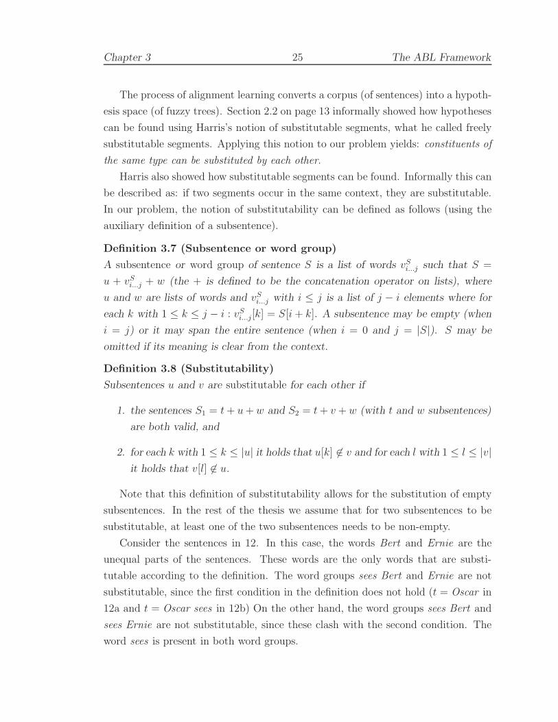
Definition 3.8 (Substitutability)
Subsentences u and v are substitutable for each other if
1. the sentences S1 = t+ u+ w and S2 = t+ v + w (with t and w subsentences)
are both valid, and
2. for each k with 1 ≤ k ≤ |u| it holds that u[k] 6∈ v and for each l with 1 ≤ l ≤ |v|
it holds that v[l] 6∈ u.
Note that this definition of substitutability allows for the substitution of empty
subsentences. In the rest of the thesis we assume that for two subsentences to be
substitutable, at least one of the two subsentences needs to be non-empty.
Consider the sentences in 12. In this case, the words Bert and Ernie are the
unequal parts of the sentences. These words are the only words that are substi-
tutable according to the definition. The word groups sees Bert and Ernie are not
substitutable, since the first condition in the definition does not hold (t = Oscar in
12a and t = Oscar sees in 12b) On the other hand, the word groups sees Bert and
sees Ernie are not substitutable, since these clash with the second condition. The
word sees is present in both word groups.

Chapter 3 26 The ABL Framework
(12) a. Oscar sees Bert
b. Oscar sees Ernie
The advantage of this notion of substitutability is that the substitutable word
groups can be found easily by searching for unequal parts of sentences. Section 4.1
will show how exactly the unequal parts (and thus the substitutable parts) between
two sentences can be found.
In Harris’s definition of substitutability it is unclear whether equal words may
occur in substitutable word groups. Definition 3.8 clearly states that the two substi-
tutable subsentences may not have any words in common. This definition is equal to
Harris’s if he meant to exclude substitutable subsentences with words in common,
or definition 3.8 is much stronger than Harris’s if he did mean to allow equal words
in substitutable word groups.
Harris used an informant to test whether a sentence is valid or not: “[I]f our
informant accepts [the sentence] or if we hear an informant say [the sentence], . . . ,
then we say [the word groups] are mutually substitutable”(Harris, 1951, p. 31).
However, in an unsupervised structure bootstrapping system there is no informant.
The only information about the language is stored in the corpus. Therefore, we
consider the validity of a sentence as follows.
Theorem 3.9 (Validity)
A sentence S is valid if an occurrence of S can be found in the corpus.
The definition of substitutability allows us to test if two subsentences are sub-
stitutable. If two subsentences are substitutable, they may be replaced by each
other and still retain a valid sentence. With this in mind, a more general version
of the definition of substitutability can be given. This version can test for multiple
substitutable subsentences simultaneously.
Definition 3.10 (Substitutability (general case))
Subsentences u1, u2, . . . , un and v1, v2, . . . , vn are pairwise substitutable for each
other if the sentences S1 = s1 + u1 + s2 + u2 + s3 + · · · + sn + un + sn+1 and
S2 = s1 + v1 + s2 + v2 + s3 + · · ·+ sn + vn + sn+1 are both valid and for each k with
1 ≤ k ≤ |n| the sentences T1 = sk + uk + sk+1 and T2 = sk + vk + sk+1 indicate that
uk and vk are substitutable for each other if T1 and T2 would be valid.
The idea behind substitutability is that two substitutable subsentences can be
replaced by each other. This is directly reflected in the general definition of sub-
stitutability. Sentence S1 can be transformed into sentence S2 by replacing substi-
Chapter 3 27 The ABL Framework
tutable subsentences. This transformation is accomplished by substituting pairs of
subsentences exactly as in the simple case.
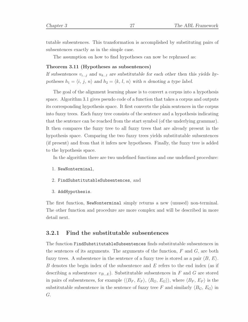
The assumption on how to find hypotheses can now be rephrased as:
Theorem 3.11 (Hypotheses as subsentences)
If subsentences vi...j and uk...l are substitutable for each other then this yields hy-
potheses h1 = 〈i, j, n〉 and h2 = 〈k, l, n〉 with n denoting a type label.
The goal of the alignment learning phase is to convert a corpus into a hypothesis
space. Algorithm 3.1 gives pseudo code of a function that takes a corpus and outputs
its corresponding hypothesis space. It first converts the plain sentences in the corpus
into fuzzy trees. Each fuzzy tree consists of the sentence and a hypothesis indicating
that the sentence can be reached from the start symbol (of the underlying grammar).
It then compares the fuzzy tree to all fuzzy trees that are already present in the
hypothesis space. Comparing the two fuzzy trees yields substitutable subsentences
(if present) and from that it infers new hypotheses. Finally, the fuzzy tree is added
to the hypothesis space.
In the algorithm there are two undefined functions and one undefined procedure:
1. NewNonterminal,
2. FindSubstitutableSubsentences, and
3. AddHypothesis.
The first function, NewNonterminal simply returns a new (unused) non-terminal.
The other function and procedure are more complex and will be described in more
detail next.
3.2.1 Find the substitutable subsentences
The function FindSubstitutableSubsentences finds substitutable subsentences in
the sentences of its arguments. The arguments of the function, F and G, are both
fuzzy trees. A subsentence in the sentence of a fuzzy tree is stored as a pair 〈B, E〉.
B denotes the begin index of the subsentence and E refers to the end index (as if
describing a subsentence vB...E). Substitutable subsentences in F and G are stored
in pairs of subsentences, for example 〈〈BF , EF 〉, 〈BG, EG〉〉, where 〈BF , EF 〉 is the
substitutable subsentence in the sentence of fuzzy tree F and similarly 〈BG, EG〉 in
G.

Chapter 3 28 The ABL Framework
Algorithm 3.1 Alignment learning
func AlignmentLearning(U : corpus): hypothesis space# The sentences in U will be used to find hypothesesvar S: sentence,
F , G: fuzzy tree,H : set of hypotheses,SS: list of pairs of pairs of indices in a sentence,PSS: pair of pairs of indices in a sentence,BF , EF , BG, EG: indices in a sentence,N : non-terminal,D: hypothesis space
beginforeach S ∈ U do
H := {〈0, |S|, startsymbol〉}F := 〈S, H〉foreach G ∈ D do
SS := FindSubstitutableSubsentences(F , G)foreach PSS ∈ SS do
〈〈BF , EF 〉, 〈BG, EG〉〉 := PSSN := NewNonterminal() # Return a new (unused) non-terminalAddHypothesis(〈BF , EF , N〉, F ) # Add to set of hypotheses of FAddHypothesis(〈BG, EG, N〉, G)
ododD := D + F # Add F to D
odreturn D
end.
Using different methods to find the substitutable subsentences results in different
instances of the alignment learning phase. Three different methods will be described
in section 4.1 on page 36. For now, let us assume that there exists a method that
can find substitutable subsentences.
3.2.2 Insert a hypothesis in the hypothesis space
The procedure AddHypothesis adds its first argument, a hypothesis in the form
〈b, e, n〉 to the set of hypotheses of its second argument (a fuzzy tree). However,
there are some cases in which simply adding the hypothesis to the set does not
exactly result in the expected structure.
In total, three distinct cases have to be considered. Assume that the procedure

Chapter 3 29 The ABL Framework
is called to insert hypothesis hF = 〈BF , EF , N〉 into fuzzy tree F and next, hG =
〈BG, EG, N〉 is inserted in G. In the algorithm, hypotheses are always added in
pairs, since substitutable subsentences always occur in pairs. The three cases will
be described with help from the following definition.
Definition 3.12 (Equal and equivalent hypotheses)
Two hypotheses h1 = 〈b1, e1, n1〉 and h2 = 〈b2, e2, n2〉 are called equal when b1 = b2,
e1 = e2, and n1 = n2. The hypotheses h1 and h2 are equivalent when b1 = b2 and
e1 = e2, but n1 = n2 need not be true.
1. The sets of hypotheses of both F and G do not contain hypotheses equivalent
to hF and hG respectively.
2. The set of hypotheses of F already contains a hypothesis equivalent to hF or
the set of hypotheses of G already contains a hypothesis equivalent to hG.
3. The sets of hypothesis of both F and G already contain hypotheses equivalent
to hypotheses hF and hG respectively.
Let us consider the first case. Both F and G receive completely new hypotheses.
This occurs for example with the fuzzy trees in 13.2
(13) a. [Oscar sees Bert]1
b. [Oscar sees Big Bird]1
In this case, the subsentences denoting Bert and Big Bird are substitutable for each
other, so a new non-terminal is chosen (2 in this case) and the hypotheses 〈2, 3, 2〉
in fuzzy tree 13a and 〈2, 4, 2〉 in fuzzy tree 13b are inserted in the respective sets
of hypotheses of the fuzzy trees. This results in the fuzzy trees as shown in 14 as
expected.
(14) a. [Oscar sees [Bert]2]1
b. [Oscar sees [Big Bird]2]1
The second case is slightly more complex. Consider the fuzzy trees in 15.
(15) a. [Oscar sees [Bert]2]1
b. [Oscar sees Big Bird]12In this thesis, non-terminals are natural numbers starting from 1, which is also the start
symbol. New non-terminals are introduced by taking the next lowest, unused natural number.

Chapter 3 30 The ABL Framework
Since hypotheses are found by considering the plain sentences only, the hypotheses
〈2, 3, 3〉 and 〈2, 4, 3〉 should be inserted respectively in the sets of hypotheses of
fuzzy trees 15a and 15b. However, the first fuzzy tree already has a hypothesis
equivalent to the new one.
Finding the hypotheses in fuzzy trees 15 indicates that Bert and Big Bird might
(in the end) be constituents of the same type. Therefore, both should receive the
same non-terminal. This can be achieved in two similar ways. One way is by adding
the hypothesis 〈2, 4, 2〉 to fuzzy tree 15b instead of 〈2, 4, 3〉 (its non-terminal is
equal to the non-terminal of the existing hypothesis) and no hypothesis is added
to 15a. This yields fuzzy trees:
(16) a. [Oscar sees [Bert]2]1
b. [Oscar sees [Big Bird]2]1
The other way is to insert the hypotheses in the regular way (overriding the
existing 〈2, 3, 2〉 in the fuzzy tree of 15a)
(17) a. [Oscar sees [Bert]2+3]1
b. [Oscar sees [Big Bird]3]1
Then all occurrences of non-terminal 2 in the entire hypothesis space are replaced
by non-terminal 3, again resulting in the fuzzy trees of 16.
The third case (where hypotheses are found that are equivalent to existing hy-
potheses in both fuzzy trees), falls into two subcases.
The first subcase is when the two original hypotheses already have the same
type. This is depicted in fuzzy trees 18.
(18) a. [Oscar sees [Bert]2]1
b. [Oscar sees [Big Bird]2]1
Since it is already known that Bert and Big Bird are hypotheses of the same type,
nothing has to be changed and the hypotheses do not even need to be inserted in
the sets of hypotheses.
However, the second subcase is more difficult. Consider the following fuzzy trees:
(19) a. [Oscar sees [Bert]2]1
b. [Oscar sees [Big Bird]3]1

Chapter 3 31 The ABL Framework
It is now known that Bert and Big Bird should have the same type, because the
tuples 〈2, 3, 4〉 and 〈2, 4, 4〉 are being inserted in the respective sets of hypotheses.
In other words, it is known that the non-terminals 2 and 3 both describe the same
type. Therefore, types 2 and 3 can be merged and all occurrences of both types in
the entire hypothesis space can be updated.
3.2.3 Clustering
In the previous section, it was assumed that word groups in the same context are
always of the same type. The assumption that if there is some evidence that word
groups occur in the same context then they also have the same non-terminal type,
might be too strong (and indeed it is, as will be shown below). However, this is just
one of the many ways of merging non-terminal types.
In fact, the merging of non-terminal types can be seen as a sub-phase of the
alignment learning phase. An instantiation based on the assumption made in the
previous section, namely that hypotheses which occur in the same context always
have the same non-terminal type, is only one possible instantiation of this phase. In
section 7.3, another instantiation is discussed. It is important to remember that the
assumption of the previous section is in no way a feature of the ABL framework, it
is merely a feature of one of its instantiations.
All systems in this thesis use the instantiation that merges types when two hy-
potheses with different types occur in the same context. This assumption influences
one of the selection learning instantiations and additionally, the qualitative evalu-
tion relies on this assumption, although similar results may be found when other
cluster methods are used.
The assumption that hypotheses in the same context always have the same non-
terminal type is not necessarily always true, as has been shown by Pinker (see
section 2.5.2.2 on page 19). Consider the following fuzzy trees:
(20) a. [Ernie eats well]1
b. [Ernie eats biscuits]1
In this case, biscuits is a noun and well is an adjective. However, ABL will con-
clude that both are of the same type. Since well and biscuits are substitutable
subsentences, they will be contained in two hypotheses with the same non-terminal.
Merging non-terminals as described in the previous section assumes that when
there is evidence that two non-terminals describe the same type, they are merged.

Chapter 3 32 The ABL Framework
However, finding hypotheses merely indicates that the possibility exists that a con-
stituent occurs there. Furthermore, it indicates that a constituent with a certain
type occupies that context. Simply merging non-terminals assumes that hypotheses
are actually constituents and that the evidence is completely correct.
A better method of merging non-terminals, which also solves Pinker’s problem,
would only merge types when enough evidence, for example in the form of frequencies
of contexts, is found. For example, types could be clustered when the hypotheses
are chosen to be correct and all hypotheses having one of the two types occur mostly
in the same contexts. Section 7.3 will discuss this in more detail.
3.3 Selection learning
The goal of the selection learning phase is to remove overlapping hypotheses from
the hypothesis space. Now that a more formal framework of hypotheses is available,
it is easy to define exactly what overlapping hypotheses are:
Definition 3.13 (Overlapping hypotheses)
Two hypotheses hi = 〈bi, ei, ni〉 and hj = 〈bj , ej , nj〉 overlap (written as hi ≬ hj)
iff (bi < bj < ei < ej) or (bj < bi < ej < ei). (Overlap between hypotheses from
different fuzzy trees is undefined.)
An example of overlapping hypotheses can be found in 21, which is the same
fuzzy tree as in 7b. It contains two hypotheses (〈0, 3, X1〉 and 〈2, 5, X2〉) which
overlap, since 0 < 2 < 3 < 5.
(21)︷ ︸︸ ︷
[X1Big Bird
︸ ︷︷ ︸[X2
throws]X1the apple]X2
The fuzzy trees generated by the alignment learning phase closely resemble the
normal notion of tree structures. The only difference is that fuzzy trees can have
overlapping hypotheses. Regular trees never have this property.
Definition 3.14 (Tree)
A tree T = 〈S, C〉 is a fuzzy tree such that for each hi, hj ∈ C : ¬(hi ≬ hj). The
hypotheses in a tree are called constituents.
Similarly, where a collection of fuzzy trees is called a hypothesis space, a collec-
tion of trees is a treebank.
Definition 3.15 (Treebank)
A treebank B is a list of trees.
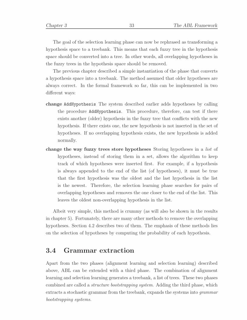
Chapter 3 33 The ABL Framework
The goal of the selection learning phase can now be rephrased as transforming a
hypothesis space to a treebank. This means that each fuzzy tree in the hypothesis
space should be converted into a tree. In other words, all overlapping hypotheses in
the fuzzy trees in the hypothesis space should be removed.
The previous chapter described a simple instantiation of the phase that converts
a hypothesis space into a treebank. The method assumed that older hypotheses are
always correct. In the formal framework so far, this can be implemented in two
different ways:
change AddHypothesis The system described earlier adds hypotheses by calling
the procedure AddHypothesis. This procedure, therefore, can test if there
exists another (older) hypothesis in the fuzzy tree that conflicts with the new
hypothesis. If there exists one, the new hypothesis is not inserted in the set of
hypotheses. If no overlapping hypothesis exists, the new hypothesis is added
normally.
change the way fuzzy trees store hypotheses Storing hypotheses in a list of
hypotheses, instead of storing them in a set, allows the algorithm to keep
track of which hypotheses were inserted first. For example, if a hypothesis
is always appended to the end of the list (of hypotheses), it must be true
that the first hypothesis was the oldest and the last hypothesis in the list
is the newest. Therefore, the selection learning phase searches for pairs of
overlapping hypotheses and removes the one closer to the end of the list. This
leaves the oldest non-overlapping hypothesis in the list.
Albeit very simple, this method is crummy (as will also be shown in the results
in chapter 5). Fortunately, there are many other methods to remove the overlapping
hypotheses. Section 4.2 describes two of them. The emphasis of these methods lies
on the selection of hypotheses by computing the probability of each hypothesis.
3.4 Grammar extraction
Apart from the two phases (alignment learning and selection learning) described
above, ABL can be extended with a third phase. The combination of alignment
learning and selection learning generates a treebank, a list of trees. These two phases
combined are called a structure bootstrapping system. Adding the third phase, which
extracts a stochastic grammar from the treebank, expands the systems into grammar
bootstrapping systems.

Chapter 3 34 The ABL Framework
It is possible to extract different types of stochastic grammars from a treebank.
Section 4.3 on page 53 will describe how two different types of grammar can be ex-
tracted. The next two sections go into the advantages of extracting such a grammar
from the treebank.
3.4.1 Comparing grammars
Evaluating grammars can be done by comparing constituents in sentences parsed by
the different grammars (Black et al., 1991).3 The grammars are compared against a
given treebank, which is considered completely correct, a gold standard. From the
treebank, a corpus is extracted. The sentences in the corpus are parsed using both
grammars. This results in two new treebanks (one generated by each grammar) and
the original treebank. The constituents in the new treebanks that can also be found
in the gold standard treebank are counted. Using these numbers from both parsed
treebanks, evaluation metrics such as precision and recall of the two grammars can
be computed and the grammars are (indirectly) compared against each other.
A similar approach will be taken when evaluating the different alignment and
selection learning phases in chapter 5. Instead of parsing the sentences with a
grammar, the trees are generated by the alignment and selection learning phases.
In this case, there is never actually a grammar present. The structure is built during
the two phases.
When a grammar is extracted from the trees generated by alignment and se-
lection learning, this grammar can be evaluated in the normal way. Furthermore,
the grammar can be evaluated against other grammars (for example, grammars
generated by other grammar bootstrapping systems).
The parseABL system, which is the ABL system extended with a grammar
extraction phase, returns a grammar as well as a structured version of the plain
corpus. The availability of a grammar is not the only advantage of this extended
system. The selection learning phase also benefits from the grammar extraction
phase, as will be explained in the next section.
3.4.2 Improving selection learning
The main idea behind the probabilistic selection learning methods is that the most
probable constituents (which are to be selected from the set of hypotheses) should
3Grammars can also be evaluated by formally comparing the grammars in terms of generativepower. However, in this thesis, the emphasis will be on indirectly comparing grammars.

Chapter 3 35 The ABL Framework
be introduced in the tree. The probability of the combination of constituents is
computed from the probabilities of its parts (extracted from the hypothesis space).
The probability of each possible combination of (overlapping and non-overlapping)
hypotheses should be computed, but the next chapter will show that this is diffi-
cult. In practice, only the overlapping hypotheses are considered for deletion. This
assumes that non-overlapping hypotheses are always correct. However, even non-
overlapping hypotheses may be incorrect.
Reparsing the plain sentences with an extracted grammar may find other, more
probable parses. This implies that more probable constituents will be inserted in
the sentences. Although the (imperfect) selection learning phase still takes place,
the grammar extraction/parsing phase simulates selection learning, reconsidering all
hypotheses.
(22) a. . . . from [Bert’s house]2 to [Sesame Street]3
b. . . . from [Sesame Street]2 to [Ernie’s room]3
Another problem that can be solved by extracting a grammar from the treebank
and then reparsing the plain sentences is depicted in example 22. In these sentences
from and to serve as “boundaries”. Hypotheses are found between these boundaries
and hypotheses between from and to are always of type 2 and hypotheses after to
are of type 3. However, Sesame Street can now have two types depending on the
context. This may be correct if type 2 is considered as a “from-noun phrase” and
type 3 as a “to-noun phrase”, but normally Sesame Street should have only one type
(e.g. a noun phrase).
Extracting a grammar and reparsing the plain sentences with this grammar may
solve this problem. When for example Sesame Street occurs more often with type
2 than with type 3, reparsing the subsentence Sesame Street will receive type 2 in
both cases.4 Finding more probable constituents can also happen on higher levels
with non-lexicalised grammar rules.
Note that reparsing not always solves this problem. If for example hypotheses
with type 2 are more probable in one context and hypotheses with type 3 are more
probable in the other context, the parser will still find the parses of 22.
It can be expected that reparsing the sentences will improve the resulting tree-
bank. A stochastic grammar contains probabilistic information about the possible
contexts of hypotheses, in contrast to the selection learning phase which only uses
local probabilistic information (i.e. counts).
4This occurs when for example to and from both have the same type label and there is agrammar rule describing a simple prepositional phrase.
Chapter 4
Instantiating the PhasesDo you still think you can control the game by brute force?
— Shiwan Khan
(tilt message in “the Shadow” pinball machine)
This chapter will discuss several instances for each of ABL’s phases. Firstly, three
different instances of the alignment learning phase will be described, followed by
three different selection learning methods. Finally, two different grammar extraction
methods will be given.
4.1 Alignment learning instantiations
The first phase of ABL aligns pairs of sentences against each other, where unequal
parts of the sentences are considered hypotheses. In algorithm 3.1 on page 28, the
function FindSubstitutableSubsentences, which finds unequal parts in a pair of
sentences, is still undefined. In the previous chapter it was assumed that such a
function exists, but no further details were given.
In this section, three different implementations of this function are discussed.
The first two are based on the edit distance algorithm by Wagner and Fischer
(1974).1 This algorithm finds ways to convert one sentence into another, from
which equal and unequal parts of the sentences can be found. The third method
1Apparently, this algorithm has been independently discovered by several researchers at roughlythe same time (Sankoff and Kruskal, 1999).
36

Chapter 4 37 Instantiating the Phases
finds the substitutable subsentences by considering all possible conversions if there
exists more than one.
4.1.1 Alignment learning with edit distance
The edit distance algorithm consists of two distinct phases (as will be described
below). The first phase finds the edit or Levenshtein distance between two sentences
(Levenshtein, 1965).
Definition 4.1 (Edit distance)
The edit distance between two sentences is the minimum edit cost2 needed to trans-
form one sentence into the other.
When transforming one sentence into the other, words unequal in both sentences
need to be converted. Normally, three edit operations are distinguished: insertion,
deletion, and substitution, even though other operations may be defined. Matching
of words is not considered an edit operation, although it works exactly the same.
Each of the edit operations have an accompanying cost, described by the prede-
fined cost function γ. When one sentence is transformed into another, the cost of
this transformation is the sum of the costs of the separate edit operations. The edit
distance is now the cost of the “cheapest” way to transform one sentence into the
other.
The edit distance between two sentences, however, does not yield substitutable
subsentences. The second phase of the algorithm gives an edit transcript, which is
a step closer to the wanted information.
Definition 4.2 (Edit transcript)
An edit transcript is a list of labels denoting the possible edit operations, which
describes a transformation of one sentence into the other.
An example of an edit transcript can be found in figure 4.1. In this figure INS
denotes an insertion, DEL means deletion, SUB stands for substitution and MAT
is a match.
Another way of looking at the edit transcript is an alignment.
Definition 4.3 (Alignment)
An alignment of two sentences is obtained by first inserting chosen spaces, either
into or at the ends of the sentences, and then placing the two resulting sentences one
2Gusfield (1997) calls this version of edit distance, operation-weight edit distance.

Chapter 4 38 Instantiating the Phases
Figure 4.1 Example edit transcript and alignment
Edit transcript: INS MAT MAT SUB MAT DELSentence 1: Monsters like tuna fish sandwichesSentence 2: All monsters like to fish
above the other so that every word or space in either sentence is opposite a unique
character or a unique space in the other string.
Edit transcripts and alignments are simply alternative ways of writing the same
notion. From an edit transcript it is possible to find the corresponding alignment
and vice versa (as can be seen in figure 4.1).
Finding indices of words that are equal in two aligned sentences is easy. Words
that are located above each other and that are equal in the alignment are called
links.
Definition 4.4 (Link)
A link is a pair of indices⟨iS, jT
⟩in two sentences S and T , such that S[iS] = T [jT ]
and S[iS] is above T [jT ] in the alignment of the two sentences.
In the example in figure 4.1, 〈1, 2〉, 〈2, 3〉, and 〈4, 5〉 are the links (when indices
of the words in the sentences start counting with 1). The first link describes the
word monsters, the second like, and the third describes fish.
Links describe which words are equal in both sentences. Combining the adjacent
links results in equal subsentences. Two links 〈i1, j1〉 and 〈i2, j2〉 are adjacent when
i1 − i2 = j1 − j2 = ±1. For example, the pairs of indices 〈1, 2〉 and 〈2, 3〉 are
adjacent, since 1− 2 = −1 and so is 3− 2. Links 〈2, 3〉 and 〈4, 5〉 are not adjacent,
since 2− 4 = −2 as is 3− 5.
From the maximal combination of adjacent links it is straightforwards to con-
struct a word cluster.
Definition 4.5 (Word cluster)
A word cluster is a pair of subsentences aSi...j and bTk...l of the same length where
aSi...j = bTk...l and S[i− 1] 6= T [k − 1] and S[j + 1] 6= T [l + 1].
Note that each maximal combination of adjacent links is automatically a word
cluster, but since sentences can sometimes be aligned in different ways, a word
cluster need not consists of links.3
3Equal words in two sentences are only called links when one is above the other in a certain
alignment.

Chapter 4 39 Instantiating the Phases
The subsentences in the form of word clusters describe parts of the sentences that
are equal. However, the unequal subsentences are needed as hypotheses. Taking the
complement of the word clusters yields exactly the set of unequal subsentences.
Definition 4.6 (Complement (of subsentences))
The complement of a list of subsentences [aSi1...i2, aSi3...i4
, . . . , aSin−1...in] is the list of
non-empty subsentences [bS0...i1, bSi2...i3
, . . . bSin...|S|].
The definition of the complement of subsentences implies that bS0...i1 + aSi1...i2 +
bSi2...i3 + aSi3...i4 + · · ·+ aSin−1...in+ bSin...|S| = S and that bS0...i1 is not present when i1 = 0
and bSin...|S| is not present when in = |S|.
To summarise, the function FindSubstitutableSubsentences is implemented
using the edit distance algorithm. This algorithm finds a list of pairs of indices where
words are equal in both sentences. From this list, word clusters are constructed,
which describe subsentences that are equal in both sentences. The complement of
these subsentences is then returned as the result of the function.
4.1.1.1 The edit distance algorithm
The edit distance algorithm makes use of a technique called dynamic programming
(Bellman, 1957). “For a problem to be solved by [the dynamic programming tech-
nique], it must be capable of being divided repeatedly into subproblems in such a
way that identical subproblems arise again and again” (Russell and Norvig, 1995).
The dynamic programming approach consists of three components.
1. recurrence relation
2. tabular computation
3. traceback
A recurrence relation describes a recursive relationship between a solution and
the solutions of its subproblems. In the case of the edit distance this comes down
to the following. When computing the edit cost between sentences A and B, D(i, j)
denotes the edit cost of subsentences uA0...i and vB0...j . The recurrence relation is then
defined as
D(i, j) = min
D(i− 1, j) + γ(A[i] → ǫ)
D(i, j − 1) + γ(ǫ → B[j])
D(i− 1, j − 1) + γ(A[i] → B[j])

Chapter 4 40 Instantiating the Phases
In this relation, γ(X → Y ) returns the edit cost of substituting X into Y , where
substituting X into the empty word (ǫ) is the same as deleting X and substituting
the empty word into Y means inserting Y . γ(X → X) does not normally count as
a substitution; the two words match.
Next to the recurrence relation, base conditions are needed when no smaller
indices exist. Here, the base conditions for D(i, j) are D(i, 0) = i ∗ γ(A[i] → ǫ) and
D(0, j) = j∗γ(ǫ → B[j]). These base conditions mean that it takes i deletions to get
from the subsentence uA0...i to the empty sentence and j insertions to construct the
subsentence vB0...j from the empty sentence. Note that this implies that D(0, 0) = 0.
Using the base conditions and the recurrence relation, a table is filled with the
edit costs D(i, j). In each entry (i, j) in the matrix, the value D(i, j) is stored.
Computing an entry in the matrix (apart from the entries D(i, 0) with 0 ≤ i ≤ |A|
and D(0, j) with 0 ≤ j ≤ |B| which are covered by the base conditions), is done
using the recurrence relation. The recurrence relation only uses information from
the direct left, upper, and upper-left entries in the matrix. An overview of the
algorithm that fills the matrix can be found in algorithm 4.1.
As an important side note, one would expect that if the order of the two sentences
that are to be aligned is reversed, all INSs will be DELs and vice versa. Matching
words still match and substituted words still need to be substituted, which would
lead to the same alignment and thus to the same substitutable subsentences. How-
ever, reversing the sentences may in some specific cases find different hypotheses.
To see how this works, consider the sentences in 23. If the algorithm chooses to link
Bert (when the sentences are in this order) since it occurs as the first word that can
be linked in the first sentence, it will choose to link Ernie when the sentences are
given in the other order (second sentence first and first sentence second), since Ernie
is the first word in the first sentence that can be linked then. The problem lies in
that the computation of the minimum cost of the three edit operations is done in a
fixed order, where multiple edit operations can return the same cost.
(23) a. Bert sees Ernie
b. Ernie kisses Bert
When the matrix is built, the entry D(|A|, |B|) gives the minimal edit cost to
convert sentence A into sentence B. This gives a metric that indicates how different
the two sentences are. However, the matrix also contains information on the edit
transcript of A and B.

Chapter 4 41 Instantiating the Phases
Algorithm 4.1 Edit distance: building the matrix
func EditDistanceX(A, B: sentence): matrix# A and B are the two sentences for which the edit cost will be computedvar i, j, msub, mdel, mins: integer
D: matrixbegin
D[0, 0] := 0for i := 1 to |A| do
D[i, 0] := D[i− 1, 0] + γ(A[i] → ǫ)odfor j := 1 to |B| do
D[0, j] := D[0, j − 1] + γ(ǫ → B[j])odfor i := 1 to |A| do
for j := 1 to |B| domsub := D[i− 1, j − 1] + γ(A[i] → B[j])mdel := D[i− 1, j] + γ(A[i] → ǫ)mins := D[i, j − 1] + γ(ǫ → B[j])D[i, j] := min(msub, mdel, mins)
ododreturn D
end.
The third component in dynamic programming, the traceback, finds an edit
transcript which results in the minimum edit cost. Algorithm 4.2 finds such a trace.
A trace normally describes which words should be deleted, inserted or substituted.
In algorithm 4.2, only the links in the two sentences are returned. Note that this
is a slightly edited version of Wagner and Fischer (1974). The original algorithm
incorrectly printed words that are equal and words that needed the substitution
operation.
Remember that from the links, the equal subsentences can be found. Taking the
complement of the equal subsentences yields the substitutable subsentences.
4.1.1.2 Default alignment learning
The general idea of using the edit distance algorithm to find substitutable subsen-
tences is described in the previous section. However, nothing has been said about
the cost function γ.
γ is defined to return the edit cost of its argument. For example, γ(A[i] → ǫ)

Chapter 4 42 Instantiating the Phases
Algorithm 4.2 Edit distance: finding a trace
func EditDistanceY(A, B: sentence, D: matrix): set of pairs of indices# A and B are the two sentences for which the edit cost will be computed# D is the matrix with edit cost information (build by EditDistanceX)var i, j: integer
P : set of pairs of indicesbegin
P := {}i := |A|j := |B|while (i 6= 0 and j 6= 0) do
if (D[i, j] = D[i− 1, j] + γ(A[i] → ǫ)) theni := i− 1
elsif (D[i, j] = D[i, j − 1] + γ(ǫ → B[j])) thenj := j − 1
elseif (A[i] = B[j]) then
P := P + 〈i, j〉fii := i− 1j := j − 1
fiodreturn P
end.
returns the cost of deleting A[i] (i.e. changing A[i] into the empty word) or γ(A[i] →
B[j]) is the cost of replacing A[i] by B[j].
Following Wagner and Fischer (1974), setting γ to return 1 for the insertion and
deletion operations and 2 for the substitution operation yields an algorithm that
finds the longest common subsequence of two sentences. This common subsequence
coincides with the notion of word cluster as described in the previous section.
Implementing the alignment learning phase using algorithm 3.1 on page 28 and
algorithms 4.1 and 4.2 results in an alignment instantiation which is called default
when γ is defined as follows:
• γ(X → X) = 0
• γ(X → ǫ) = 1
• γ(ǫ → X) = 1
• γ(X → Y ) = 2

Chapter 4 43 Instantiating the Phases
Figure 4.2 Example of a filled edit distance table
monsters like tuna fish sandwiches
0 1 1 2 2 3 3 4 4 5 51 2 2 3 3 4 4 5 5 6 6
all 1 2 2 3 3 4 4 5 5 6 62 1 3 4 4 5 5 6 6 7 7
monsters 2 3 1 2 2 3 3 4 4 5 53 4 2 1 3 4 4 5 5 6 6
like 3 4 2 3 1 2 2 3 3 4 44 5 3 4 2 3 3 4 4 5 5
to 4 5 3 4 2 3 3 4 4 5 55 6 4 5 3 4 4 3 5 6 6
fish 5 6 4 5 3 4 4 5 3 4 4
Figure 4.2 is an example of the edit distance algorithm with the γ function as
described above. The sentence Monsters like tuna fish sandwiches is transformed
into All monsters like to fish. The values in the upper row and left column correspond
to the base conditions. The other entries in the table have four values. The upper
left value describes the cost when substituting (or matching) the words in that row
and column plus the previous edit cost (found in the entry to the north-west). The
upper right entry describes the edit cost of insertion plus the edit cost to the north.
The lower left value is the edit cost of deletion plus the edit cost to the west. The
lower right value is the minimum of the other three values, which is also the value
stored in the actual matrix.
The bold values describe an alignment. The transcript of this alignment is found
when starting from the lower right entry in the matrix and going back (following the
bold value, which are constantly the minimum values on that point in the matrix)
to the upper left entry. The transcript is then a DEL, MAT, SUB, MAT, MAT,
INS, which is the (reversed) transcript shown in figure 4.1.
4.1.1.3 Biased alignment learning
Using the algorithm (and cost function) described above to find the dissimilar parts
of the sentences does not always result in the preferred hypotheses. As can be seen
when aligning the parts of the sentences in 24, the default algorithm generates the
alignment in 25, because Sesame Street is the longest common subsequence. Linking
Sesame Street costs 4, while linking England (shown in the sentences in 26) or to

Chapter 4 44 Instantiating the Phases
(shown in the sentences in 27) costs 6.
(24) a. . . . from Sesame Street to England
b. . . . from England to Sesame Street
(25) a. . . . from [ ]2 Sesame Street [to England]3
b. . . . from [England to]2 Sesame Street [ ]3
(26) a. . . . from [Sesame Street to]4 England [ ]5
b. . . . from [ ]4 England [to Sesame Street]5
(27) a. . . . from [Sesame Street]6 to [England]7
b. . . . from [England]6 to [Sesame Street]7
However, aligning Sesame Street results in unwanted syntactic structures. Both
to England and England to are considered hypotheses. A more preferred alignment
can be found when linking the word to.
This problem occurs every time the algorithm links words that are “too far
apart”. The relative distance between the two Sesame Streets in the two sentences
is much larger than the relative distance between the word to in both sentences.
This can be solved by biasing the γ cost function towards linking words that
have similar offsets in the sentence. The Sesame Streets reside in the beginning and
end of the sentences (the same applies to England in the alignment of sentences 26),
so the difference in offset is large. This is not the case for to; both reside roughly in
the middle.
An alternative cost function may be biased towards linking words that have a
small relative distance. This can be accomplished by letting the cost function return
a high cost when the difference of the relative offsets of the words is large. The
relative distance between the two Sesame Streets in sentences 25 is larger compared
to the relative distance between the two tos in sentences 27. Therefore the total edit
cost of sentences 27 will be less than the edit cost of sentences 25 or sentences 26.
In the system called biased , the γ function will be changed as follows:
• γ(X → X) =
∣∣∣∣
iSX|S|
−iTX|T |
∣∣∣∣∗mean(|S|, |T |) where iUW is the index of word W in
sentence U and S and T are the two sentences.

Chapter 4 45 Instantiating the Phases
• γ(X → ǫ) = 1
• γ(ǫ → X) = 1
• γ(X → Y ) = 2
If the parts of the sentences shown in 24 are the complete sentences, the edit
transcription with minimum edit cost of the alignment in 25 is [MAT, INS, INS,
MAT, MAT, DEL, DEL] with costs: 0 + 1+ 1+ 2+ 2+ 1+ 1 = 8, for the sentences
in 26 this is [MAT, DEL, DEL, DEL, MAT, INS, INS, INS] with costs: 0 + 1 + 1 +
1 + 3 + 1 + 1 + 1 = 9 and the sentences in 27 become [MAT, SUB, DEL, MAT,
SUB, INS] with costs: 0 + 2 + 1 + 1 + 2 + 1 = 7. Therefore, the alignment with to
is chosen.
The biased system does not entirely solve the problem, since in sentences similar
to those in 28 the words from and Sesame Street are linked (instead of the words
from and to as preferred).
(28) a. . . . from England to Sesame Street
b. . . . from Sesame Street where Big Bird lives to England
Additionally, the biased system will find less hypotheses, since less matches will
be found compared to the default system. Where the default system still matched
words that are relatively far apart, the biased system will not match them. Less
links and thus less word groups and hypotheses will be found.
4.1.2 Alignment learning with all alignments
Another solution to the problem of introducing incorrect hypotheses is to simply
generate all possible alignments (using an alignment algorithm that is not based on
the edit distance algorithm).4 This method is called all.
When all possible alignments are considered, the selection learning phase of ABL
has a harder job selecting the best hypotheses. Since the alignment learning finds
more alignments, more hypotheses are inserted into the hypothesis space. And
thus the selection learning phase has more to choose from. However, because the
alignment learning phase does not know which are the correct hypotheses to insert,
inserting all of them might be the best option.
4It is also possible to implement this using an adapted version of the edit distance algorithmthat keeps track of all possible alignments using a matrix with pointers.

Chapter 4 46 Instantiating the Phases
Algorithm 4.3 finds all possible alignments between two sentences. The func-
tion AllAlignments takes two sentences as arguments. The first step in the algo-
rithm finds a list of all matching terminals. This list is generated in the function
FindAllMatchingTerminals. This list contains pairs of indices of words in the two
sentences that can be linked (i.e. words that might be a link in an alignment). Note
that this list can contain crossing links (in contrast to the links found by the edit
distance algorithm).
Next, the algorithm incrementally adds each of these links into all possible align-
ments. If inserting a link in an alignment results in overlapping links within that
alignment (which is not allowed), a new alignment is introduced. In algorithm 4.3
this is the case when O 6= ∅. The first alignment is unchanged (i.e. the current link
is not inserted): P := P + (j) and the current link is added to the new alignment,
which contains all links from the first alignment which do not overlap with the cur-
rent link: P := P +(j−O+ i). This might insert alignments that are proper subsets
of other alignments in P , so before returning, these subsets need to be filtered away.
Since variable P is a set, no duplicates are introduced, so when all links are
appended to the possible alignments, P contains all possible alignments in the two
sentences.
4.2 Selection learning instantiations
Not only the alignment learning phase can have different instantiations. Selection
learning can also be done in different ways. Several different methods will be de-
scribed here. First, there is the simple, non-probabilistic method as described in
chapter 2. Next, two probabilistic methods will be described. These probabilistic
selection learning methods differ in the way probabilities of hypotheses are com-
puted.
4.2.1 Non-probabilistic selection learning
Remember that the selection learning phase should take care that no overlapping
hypotheses remain in the structure generated by the alignment learning phase. The
easy solution to this problem is to make sure that overlapping hypotheses are never
even introduced. In other words, if at some point, the system tries to insert a
hypothesis that overlaps with a hypothesis that was already present, it is rejected.
The underlying assumption in this non-probabilistic method is that a hypothesis
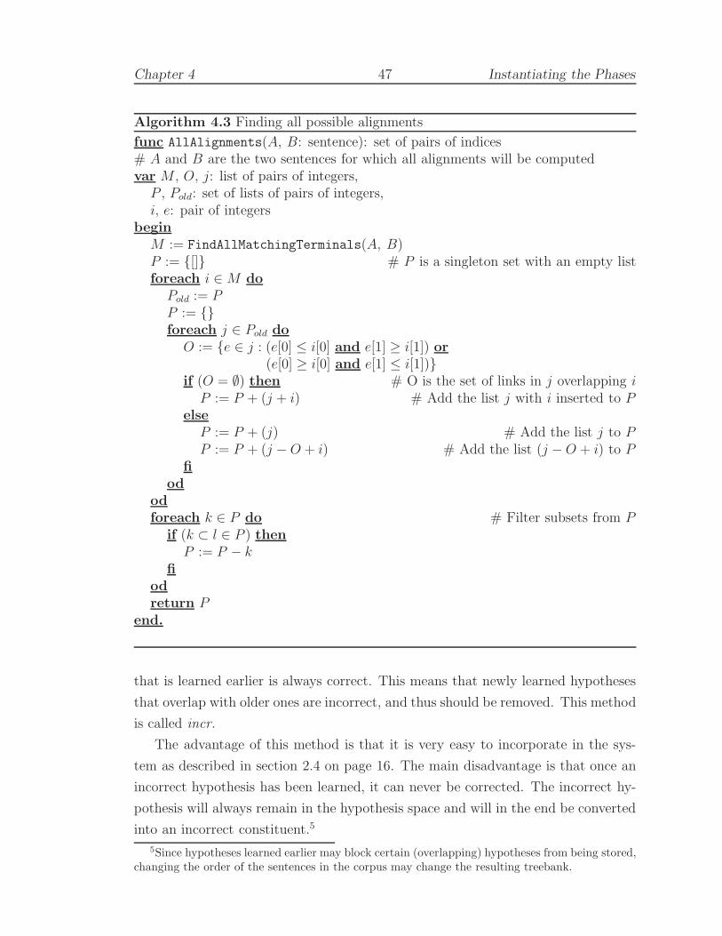
Chapter 4 47 Instantiating the Phases
Algorithm 4.3 Finding all possible alignments
func AllAlignments(A, B: sentence): set of pairs of indices# A and B are the two sentences for which all alignments will be computedvar M , O, j: list of pairs of integers,
P , Pold: set of lists of pairs of integers,i, e: pair of integers
beginM := FindAllMatchingTerminals(A, B)P := {[]} # P is a singleton set with an empty listforeach i ∈ M do
Pold := PP := {}foreach j ∈ Pold do
O := {e ∈ j : (e[0] ≤ i[0] and e[1] ≥ i[1]) or(e[0] ≥ i[0] and e[1] ≤ i[1])}
if (O = ∅) then # O is the set of links in j overlapping iP := P + (j + i) # Add the list j with i inserted to P
elseP := P + (j) # Add the list j to PP := P + (j − O + i) # Add the list (j −O + i) to P
fiod
odforeach k ∈ P do # Filter subsets from P
if (k ⊂ l ∈ P ) thenP := P − k
fiodreturn P
end.
that is learned earlier is always correct. This means that newly learned hypotheses
that overlap with older ones are incorrect, and thus should be removed. This method
is called incr.
The advantage of this method is that it is very easy to incorporate in the sys-
tem as described in section 2.4 on page 16. The main disadvantage is that once an
incorrect hypothesis has been learned, it can never be corrected. The incorrect hy-
pothesis will always remain in the hypothesis space and will in the end be converted
into an incorrect constituent.5
5Since hypotheses learned earlier may block certain (overlapping) hypotheses from being stored,changing the order of the sentences in the corpus may change the resulting treebank.

Chapter 4 48 Instantiating the Phases
The assumption that hypotheses learned earlier are correct may perhaps be only
likely for human language learning. It so happens that the type of sentences in a cor-
pus are generally not comparable to the type of sentences human hear when they are
learning a language. Furthermore, the implication that once an incorrect hypothesis
has been learned, it can never be corrected, is (cognitively) highly implausible.
4.2.2 Probabilistic selection learning
To solve the disadvantage of the first method, probabilistic selection learning meth-
ods have been implemented. The probabilistic selection learning methods select the
combination of hypotheses with the highest combined probability. These methods
are accomplished after the alignment learning phase, since more specific information
(in the form of better counts) can be found at that time.
First of all, the probability of each hypothesis has to be computed. This can be
accomplished in several ways. Here, two different methods will be considered. By
combining the probabilities of the single hypotheses, the combined probability of a
set of hypotheses can be found.
Different ways of computing the probability of a hypothesis will be discussed first,
followed by a description on how the probability of a combination of hypotheses can
be computed.
4.2.2.1 The probability of a hypothesis
The probability of a hypothesis is the chance that a hypothesis is drawn from the
entire space of possible hypotheses. If it is assumed that the alignment learning phase
generates the space of hypotheses, the probability of a hypothesis can be computed
by counting the number of times that the specific hypothesis occurs in hypotheses
generated by alignment learning. The hypotheses generated by alignment learning
make up the hypothesis universe.6
Definition 4.7 (Hypothesis universe)
The hypothesis universe is the union of all sets of hypotheses of the fuzzy trees in
a hypothesis space. In other words, the hypothesis universe UD of hypothesis space
D is UD =⋃
F=〈SF , HF 〉∈D HF .
6Remember (definition 3.6) that a hypothesis space is a set of fuzzy trees. The hypothesisuniverse is the combination of the hypotheses of all fuzzy trees in a certain hypothesis space.

Chapter 4 49 Instantiating the Phases
The probability that a certain hypothesis h occurs in a hypothesis universe D is
its relative frequency under the assumption of the uniform distribution:
PU(h)def=
|h|
|U |
All hypotheses in a hypothesis universe are unique. Within the set of hypotheses
of a fuzzy tree they are unique, and all are indexed with their fuzzy tree, so hypothe-
ses of different fuzzy trees can never be the same. This means that the previous
formula can be rewritten as:
PU(h) =1
|U |
The numerator becomes 1, since each hypothesis only occurs once and the denom-
inator is exactly the total number of hypotheses in the hypothesis universe. The
probability of a hypothesis is the same for all hypotheses.
The fact that each hypothesis has an equal probability of occurring in the hy-
pothesis universe, does not help in selecting the better hypotheses. Hypotheses
receive the same probabilities, because all hypotheses are unique.
Even though hypotheses are unique, it can be said that certain hypotheses are
equal when concentrating on only certain aspects of the hypotheses. Instead of
obliging all properties of two hypotheses to be the same, taking only certain prop-
erties of a hypothesis into account when deciding which hypotheses are the same
relaxes the equality relation.
PU(h) describes the probability of hypothesis h in the hypothesis universe U .
By grouping hypotheses with a certain property, the probability of a hypothesis is
calculated relative to the subset of hypotheses that all have that same property. One
way of grouping hypotheses is by their yield.
Definition 4.8 (Yield of a hypothesis)
The yield of a hypothesis yield(hS) is the list of words (in the form of a subsentence)
grouped together by the hypothesis. If hS = 〈b, e, n〉 then yield(hS) = vSb...e.
The first probabilistic method computes the probability of a hypothesis by count-
ing the number of times the subsentence described by the hypothesis has occurred
as a hypothesis in the hypothesis universe, normalised by the total number of hy-
potheses. Thus the probability of a hypothesis h in hypothesis universe U can be
computed using the following formula.
PUleaf (h) =
|h′ ∈ U : yield(h′) = yield(h)|
|U |

Chapter 4 50 Instantiating the Phases
This method is called leaf since we count the number of times the leaves (i.e.
the words) of the hypothesis co-occur in the hypothesis universe as hypotheses.
The second method relaxes the equality relation in a different way. In addition
to comparing the words of the sentence delimited by the hypothesis (as in the leaf
method), this model computes the probability of a hypothesis based on the words
of the hypothesis and its type label (the function root returns the type label of a
hypothesis). This model is effectively a normalised version of Pleaf . This probabilistic
method of computing the probability of a hypothesis is called branch .
PUbranch(h) =
|h′ ∈ U : yield(h′) = yield(h) ∧ root(h′) = root(h)|
|h′′ ∈ U : root(h′′) = root(h)|
First, a partition of the hypothesis space is made by considering only hypotheses
with a certain type label. In other words, the hypothesis universe U as used in Pleaf
is partitioned into parts bounded by all possible type labels. For a certain hypothesis
h this becomes: U ′h = {h′ ∈ U : root(h′) = root(h)}, the set of hypotheses where
the root is the same as the root of h. Substituting U ′h (where h is the hypothesis for
which the probability is computed) for U in Pleaf yields Pbranch .
The two methods just described are not the only possible approaches. Another
interesting method, for example, could take into account the inner structure of a
hypothesis. In other words, the probability of a hypothesis not only depends on
the words in its yield, but also on other hypotheses that occur within the part of
the sentence encompassed by the hypothesis. Such an approach will be described in
section 7.4 on page 103.7
4.2.2.2 The probability of a combination of hypotheses
The previous section described two ways to compute the probability of a hypothesis.
Using these probabilities, it is possible to calculate the probability of a combination
of hypotheses. The combination of hypotheses with the highest probability is then
chosen to be the “correct” combination. This section describes how the probability of
a combination of hypotheses can be computed using the probabilities of the separate
hypotheses.
Since each selection of a hypothesis from the hypothesis universe is independent
7This yields a (stochastically) more precise model (taking also the information of non-terminalsinto account). However, the information contained in the hypothesis space is unreliable, since thealignment learning phase also inserts incorrect hypotheses into the hypothesis universe. In otherwords, the model tries to give more precise results based on more imprecise information from thehypothesis universe.

Chapter 4 51 Instantiating the Phases
of the previous selections, the probability of a combination of hypotheses is the
product of the probabilities of the constituents as in SCFGs (cf. (Booth, 1969)).
This means that if the separate probabilities of the hypotheses are known, the
combined probability of hypotheses h1, h2, . . . , hn can be computed as follows:
PSCFG(h1, h2, . . . , hn) =
n∏
i=1
P (hi)
However, using the product of the probabilities of hypotheses results in a trashing
effect, since the product of hypotheses is always smaller than or equal to the separate
probabilities. Since probabilities are all between 0 and 1, multiplying many proba-
bilities tends to reduce the combined probability towards 0. Consider comparing the
probability of the singleton set of the hypothesis {h1} with probability Ph1= P (h1)
to the set of hypotheses {h1, h2} with probability Ph1,h2= P (h1)P (h2). It will al-
ways hold that Ph1,h2≤ Ph1
. Thus in general, taking the product of probabilities
prefers smaller sets of hypotheses.
To eliminate this effect, a normalised method of computing the combined proba-
bility is used. According to Caraballo and Charniak (1998), the geometric mean re-
duces the trashing effect. Therefore, the probability of a set of constituents h1, . . . , hn
is computed using:
PGM (h1, . . . , hn) =n
√√√√
n∏
i=1
P (hi)
The probability of a certain hypothesis h can be computed using one of the methods
described in the previous section (Pleaf or Pbranch).
In practice, many probabilities may be multiplied, which can result in a numerical
underflow. To solve this, the logprob (i.e. the − log) of the probabilities is used. The
geometric mean can be rewritten (where LP denotes the logprob) as:
LPGM (h1, . . . , hn) =
∑n
i=1 LP (hi)
n
which shows that the geometric mean actually computes the mean of the logprob of
the hypotheses.
Using this formula effectively selects only those hypotheses that have the highest
probability (in the set). Assume the mean of a set of values is computed. If a
value higher than that mean is added to the set, the newly computed mean will
be higher, while adding a value lower than the mean will lower the resulting mean.

Chapter 4 52 Instantiating the Phases
This means that the set with (only) the lowest values will be chosen when looking
for the minimum mean. If there are more elements that have the same value,
any combination of these elements result in the same mean value (the mean of
for example [3, 3] is the same as the mean of [3]).
Although using the PGM (or the equivalent LPGM ) method eliminates the trash-
ing effect, it does not have a preference for richer structures when there are two (or
more) combinations of hypotheses that have the same probability.
To let the system have a preference for more constituents in the final tree struc-
ture when there are more possibilities with the same probability, the extended ge-
ometric mean is implemented. The only difference with the (standard) geometric
mean is that when there are more possibilities (single hypothesis or combinations of
hypotheses) with the same probability, this system selects the combination with the
most hypotheses. To indicate that the systems use the extended geometric mean, a+ is added to the name of the methods that use the extended geometric mean. For
example, using the leaf method to compute the probabilities of hypotheses and the
extended geometric mean to compute the combined probability is called leaf+ (and
similarly branch+ when using branch). If there are sets of hypotheses that have
the same probability and the same number of hypotheses, one of them is chosen at
random.
The properties of the geometric mean also explain why only the set of overlapping
hypotheses is considered when computing the most probable structure of the fuzzy
tree. In other words, hypotheses that do not overlap any other hypothesis in the
fuzzy tree are always considered correct. If all hypotheses were considered, only
the hypotheses with the highest probability will be selected. This means that many
correct hypotheses will be thrown away. (It is very probable that the hypothesis
with the start symbol will not be selected, since the probability of that hypothesis
is very small; it only occurs as often as the entire sentence occurs in the corpus.)
Previous publications also mentioned methods that used the leaf and branch
methods of computing the probabilities of hypotheses and the (standard) geometric
mean to compute the combined probabilities. These systems however did not prefer
more richly structured trees. They chose a random solution if multiple solutions were
found. Since these systems will always learn the same amount of or less structure,
they will not be considered here.
The probability of each combination of mutually non-overlapping hypotheses is
computed using a Viterbi style optimisation algorithm (Viterbi, 1967). The combi-
nation of hypotheses with the highest probability (and the lowest logprob) is selected
Chapter 4 53 Instantiating the Phases
and the overlapping hypotheses not present in this combination are removed from
the fuzzy tree.
4.3 Grammar extraction instantiations
When the selection learning phase has disambiguated the fuzzy trees, regular tree
structures remain. From these tree structures, it is possible to extract a grammar.
First, the focus is on extracting a stochastic context-free grammar (SCFG), since the
underlying grammar of the final treebank is considered context-free. Next, extract-
ing a stochastically stronger grammar type, stochastic tree substitution grammar
(STSG), is described.
4.3.1 Extracting a stochastic context-free grammar
In general, it is possible to extract grammar rules from tree structures (i.e. parsed
sentences). These grammar rules can generate the tree structures it was extracted
from. In other words, parsing the sentence with the extracted grammar can return
the same structure.8
Imagine the structured sentences as displayed in figure 4.3. These two sentences
can also be written as tree structures. Extracting a context-free grammar from the
tree structures is rather straightforward. For each node (non-terminal in the tree
structure), take the label as the left-hand side of a grammar rule. The list of direct
daughters of the node are the right-hand side of the grammar rule.
When the extracted context-free grammars are stored in a bag, the probabilities
of the grammar rules can easily be computed, which converts the context-free gram-
mar in a stochastic version. The probability of a context-free grammar rule is the
number of times the specific grammar rule occurs in the bag, divided by the total
number of grammar rules with the same non-terminal on its left-hand side. Extract-
ing a stochastic context-free grammar from the two trees, results in the SCFG in
figure 4.3.
When all grammar rules are extracted from the tree structure, the probabilities
of the grammar rules in the grammar are then computed using the following formula:
PG(s) =|s′ ∈ G : LHS(s′) = LHS(s) ∧ RHS(s′) = RHS(s)|
|s′′ ∈ G : LHS(s′′) = LHS(s)|8Since an ambiguous grammar may be extracted from a set of tree structures, it is not necessarily
the case that a structure equal to the original is assigned to the sentence.

Chapter 4 54 Instantiating the Phases
Figure 4.3 Extracting an SCFG from a tree structure
[[Bert]NP[[sees]V[Ernie]NP]VP]S[[Ernie]NP[[walks]V]VP]S
S
NP
Bert
VP
V
sees
NP
Ernie
S
NP
Ernie
VP
V
walks
S → NP VP 2/2=1VP → V NP 1/2=0.5VP → V 1/2=0.5NP → Bert 1/3=0.33NP → Ernie 2/3=0.67V → sees 1/2=0.5V → walks 1/2=0.5
In this formula, LHS(x) denotes the left-hand side of grammar rule x, while RHS(x)
denotes the right-hand side of x.
4.3.2 Extracting a stochastic tree substitution grammar
The previous section showed how a stochastic context-free grammar can be extracted
from a tree structure. This section will concentrate on extracting a stochastic tree
substitution grammar (STSG). This type of grammar can generate the same tree
structures as a context-free grammar, but is stochastically stronger (Bod, 1998).
When grammar rules, called elementary trees in an STSG, are extracted from a
tree T , each grammar rule t is in the form such that:
• t consists of more than one node
• t is connected
• except for frontier nodes of t, each node in t has the same daughter nodes as
the corresponding node in T
An example of the elementary trees in a tree structure can be found in figure 4.4.

Chapter 4 55 Instantiating the Phases
This figure contains all elementary trees that can be extracted from the first tree in
the figure. Note that the first tree is also an elementary tree (of itself).
Figure 4.4 Example elementary trees
S
NP
Bert
VP
V
sees
NP
Ernie
S
NP
Bert
VP
V NP
Ernie
S
NP
Bert
VP
V
sees
NP
S
NP
Bert
VP
V NP
S
NP
Bert
VP
S
NP VP
V
sees
NP
Ernie
S
NP VP
V NP
Ernie
S
NP VP
V
sees
NP
S
NP VP
V NP
S
NP VP
VP
V
sees
NP
Ernie
VP
V NP
Ernie
VP
V
sees
NP
VP
V NP
NP
Bert
V
sees
NP
Ernie
The description of what an elementary trees is, does not give a procedure to
actually find these. van Zaanen (1997, p. 49) gives a (slightly informal) description
of an algorithm that finds all elementary trees in a given tree.
As can be seen in figure 4.4, extracting elementary trees from one tree structure
can result in many elementary trees. When the number of trees from which elemen-

Chapter 4 56 Instantiating the Phases
tary trees are extracted becomes larger, the number of elementary trees becomes
huge. To keep the number of elementary trees within practical limits, it is possible
to set a condition on the maximum depth of the elementary trees (van Zaanen, 1997,
p. 51).
The probabilities of the elementary trees are computed similarly to the proba-
bilities of the context-free grammar rules in an SCFG:
PG(s) =|s′ ∈ G : s′ = s|
|s′′ ∈ G : root(s′′) = root(s)|
Again, root(x) denotes the root type label of the elementary tree x.
Chapter 5
Empirical ResultsAfter all the purpose of computing is insight, not numbers,
and one good way to demonstrate this is to take a situation
where the numbers are clearly less important than the insights gained.
— Knuth (1996)
This chapter will put the theory of the previous chapters into practice. Each of
the ABL systems (which are combinations of an alignment and a selection learning
instance) is evaluated. Firstly, the focus is on evaluating the alignment learning
phase, followed by a comparison of the results of both phases. Using the data gener-
ated by these systems, the grammar extraction and parsing phase of the parseABL
systems are also evaluated.
Apart from a numerical analysis, which will be described first, the learned tree-
banks generated by ABL systems are looked at in a qualitative way. The learned
treebanks contain for example constituents that closely resemble nouns and “from-
to” phrases, but also many words are roughly tagged accoring to parts-of-speech.
Furthermore, each of the generated treebanks contain recursive structures.
5.1 Quantitative results
This section first discusses the advantages and disadvantages of the method used here
to evaluate the ABL and parseABL instances. Next, the test environment, consisting
of the treebanks, metrics and learning instances used, is described. Finally, the
57

Chapter 5 58 Empirical Results
actual results of the different phases of the framework and their evaluation are
given.
5.1.1 Different evaluation approaches
Evaluating language learning systems is difficult. Usually, one of three different
evaluation methods is chosen. Here, the three methods will be described briefly
concentrating on their advantages and disadvantages.
Looks-good-to-me approach When a language learning system is evaluated us-
ing the looks-good-to-me approach, the system is applied to an unstructured
piece of text and the resulting grammar rules or structured sentences are qual-
itatively evaluated. If (intuitively) correct grammatical structures are found
in the grammar or structured sentences, the system is said to be good. Since
this is such a simple approach, it has been used to evaluate many systems,
for example those by Cook et al. (1976); Cook and Holder (1994); Finch and
Chater (1992); Grunwald (1994); Huckle (1995); Losee (1996); Scholtes and
Bloembergen (1992); Stolcke and Omohundro (1994); Vervoort (2000).
advantages The main advantage of this approach is that only unstructured
data is needed. This means that the system can easily be evaluated on
different languages without the need of structured corpora.
Another advantage is that the evaluation can focus on certain specific
syntactic constructions the system should be able to learn. Since the
evaluation is done in a qualitative way, the input data can be specialised
to show that the system can learn such constructions and the structured
output can be searched for the wanted syntax.
disadvantages It may be clear that this approach has a few disadvantages.
First of all, for the evaluation of language learning sytems using this
approach, an expert who has specific knowledge of the syntax of the
language in the test corpus is needed. The expert can tell which syntactic
structures should be present in the learned treebank and also if certain
generated structures are correct or incorrect.
This leads to the second disadvantage, that of biased evaluation. In
this approach, it is possible to pick the correctly learned grammatical
features only and leave out the incorrect ones. It will seem that the
system works well, since all grammatical structures that are shown are

Chapter 5 59 Empirical Results
correct. However, the learned treebank also contains incorrect structures
which are not shown.
Furthermore, it is difficult to compare two systems based on this ap-
proach. Imagine two language learning systems that each find some other
correct and incorrect structures. Which of the two systems is better?
The final disadvantage is that the unstructured input corpus may be
biased towards a specific system. In other words, it may be possible
to (unknowingly) feed the system only sentences that will generate the
wanted syntactic structures.
Rebuilding known grammars Another approach in evaluating language learning
systems is to let the system rebuild a known grammar. This evaluation method
starts out with a (simple) grammar, from which a set of example sentences is
generated. This set of sentences must at least represent each of the features
of the grammar once. The sentences are then fed to the learning system and
the resulting grammar is compared manually to the original grammar. If the
learned grammar is similar or equal to the original grammar then the learning
system is considered good. This evaluation approach has been used by, a.o.
Cook et al. (1976); Nakamura and Ishiwata (2000); Pereira and Schabes (1992);
Sakakibara and Muramatsu (2000); Stolcke (1994); Wolff (1996).
advantages This method has similar advantages as the looks-good-to-me ap-
proach. It does not need structured sentences to evaluate, because plain
sentences, generated by the grammar, are used to learn structure. These
grammars can be tailored to specific grammatical constructions, which
allows for a specific evaluation of certain aspects of the system.
Additionally, the looks-good-to-me approach needs an expert to indicate
whether a grammatical construction is correct or incorrect, but this is
unnecessary for this approach. If the learned grammar is similar to the
original grammar, the learning system works well.
Another advantage is that this method of evaluation yields a more ob-
jective way of comparing different language learning systems, since the
entire grammars are compared (and not only the intuitively correct parts
of the grammar). However, even then it is still difficult to say which of
two (slightly) incorrect grammars is closer to the original grammar.
disadvantages One of the disadvantages of this approach is that the evalua-
tion of the system depends heavily on the chosen grammar. Some learning

Chapter 5 60 Empirical Results
systems can rebuild certain types of grammars more easily than others;
by choosing simple grammars, the system can be shown to be better than
it really is.
The idea of a language learning system is that it finds correct structure in
real natural language data. This means that the original grammar should
be as close to the underlying grammar of natural language sentences as
possible. However, this grammar is in general not fully known.
A related problem is that the language generation model, which gener-
ates the example sentences from the grammar, is not known either. The
language generation model should create a set of sentences that describes
each of the grammatical features contained in the grammar, but if the
language learning system is designed to work on real natural language
texts (as is ABL), it should also create sentences that resemble real nat-
ural language sentences.
Compare against a treebank The third method of evaluation a language learn-
ing system, which will be used in this thesis, is to apply the system to plain
natural language sentences which are extracted from a treebank. The struc-
tured sentences generated by the language learning system are then compared
against the original structured sentences from the treebank.
There are several metrics that can be used to compare the learned tree against
the original tree structure. Most often, the recall, which gives a measure of
the completeness of the learned grammar, and the precision, which shows how
correct the learned structure is, are computed. These metrics give a gradual
indication of the performance of a learning system which allows the comparison
of two systems that find correct, but also some incorrect, structure.
This method of evaluating learning systems is, in our view, the most objective.
Lately, almost all systems are evaluated using this approach. Examples can be
found in (Brent, 1999; Brill, 1993; Clark, 2001b; Dejean, 2000; Nevado et al.,
2000).
advantages This approach does not need an expert to indicate if some con-
struction is correct or incorrect. All linguistic knowledge is already con-
tained in the original treebank. This also means that real natural lan-
guage data can be used. Of the three evaluation methods, this approach

Chapter 5 61 Empirical Results
comes closest to the evaluation of the system in the context of a real
world application.
Furthermore, this approach allows for a relatively objective comparison of
learning systems. Since several metrics can be used, gradual distinctions
between systems can be made. Precise information indicating how well
the systems perform on the treebank can be found, since the systems are
given a score even when only parts of the learned structure are correct.
disadvantages This method also has its disadvantages. The first disadvan-
tage is that a collection of structured sentences is needed. At the moment
however, structured data is only available for a limited number of lan-
guages. This severely restricts the evaluation of language independency
of the systems.
A second disadvantage is that the annotation scheme and imperfect anno-
tation influence the results. If, for example, the structure of the sentences
in the original treebank is relatively flat, but the language learning sys-
tem finds rich, deep structures, it will be penalised for that, since it learns
structure that is not present in the “correct” treebank. Suppose that for
example sentence 29a is the structured sentences in a treebank and sen-
tence 29b is the learned tree, the constituent [Big ]AP will be counted
as incorrect, since it is not present in the original treebank. However,
depending on the annotation scheme, this constituent could have been
correct. Similar things happen when the annotation of the sentences in
the original treebank contains errors.
(29) a. [[Oscar]NP [sees [Big Bird]NP]VP]S
b. [[Oscar]NP [sees [[Big]AP Bird]NP]VP]S
Evaluating language learning systems by comparing them against a treebank
is done as shown in figure 5.1. Evaluation starts off with a base treebank. The
trees in this treebank are taken to be perfectly correct, a gold standard. From each
tree in this treebank, the plain sentence (i.e. the yield of the tree) is extracted.
These sentences (contained in the plain corpus in the figure) are fed to the language
learning system and the results are stored in the learned treebank. The trees in the
learned treebank are then compared to the trees from the base treebank.
Applying the evaluation method to a language learning system indicates how
much of the structure in the original treebank is found and how much correct struc-

Chapter 5 62 Empirical Results
Figure 5.1 Evaluating a structure induction system
Basetreebank
Extractsentences
Comparetreebanks
Results
Plaincorpus
Learningsystem
Learnedtreebank
ture is generated by the system. To get an idea how good the system really is,
it needs to be compared against another system. Comparing the results of two
language learning systems against each other shows which of the two works better
(on this specific corpus). Normally, a system is compared against a baseline sys-
tem. This is usually a simple system that generates for example trees with random
structure.
5.1.2 Test environment
This section describes the settings used for testing the ABL and parseABL frame-
works. Starting with a description of the different treebanks that will be used in this
thesis, the section continues by explaining the evaluation metrics that are computed
to compare the learned tree structures against the original tree structures. Finally,
a brief overview of the tested systems will be given.
5.1.2.1 Treebanks
As mentioned in the previous section, the grammar induction systems will be applied
to the plain sentences of a structured corpus. This section will describe the treebanks
that have been used to test the ABL and parseABL systems in this thesis.
First of all, it needs to be mentioned that not many structured treebanks are
available. There is only a limited number of languages for which structured treebanks
are available. Unfortunately, to test if a grammar induction system is really language

Chapter 5 63 Empirical Results
independent, it needs to be applied to treebanks of several (different) languages.
Here, two treebanks have been used to extensively test the ABL and parseABL
systems. Results on a third treebank, the Wall Street Journal treebank, will be
discussed in a separate section. The first treebank is the Air Traffic Information
System (ATIS) treebank (Marcus et al., 1993), which is taken from the Penn tree-
bank 2. It is an English treebank containing mostly questions and imperatives on
air traffic. The sentences in 30 are some (random) samples that are found in the
treebank. The treebank consists of 577 sentences with a mean sentence length of
7.5 words per sentence. All empty constituents (and traces) that can be found in
this treebank have been removed beforehand.
(30) a. What airline is this
b. The return flight should leave at around seven pm
c. Show me the flights from Baltimore to Oakland please
The second treebank is the Openbaar Vervoer Informatie Systeem1 (OVIS) tree-
bank (Bonnema et al., 1997). This Dutch treebank, with its 10,000 trees, is larger
than the ATIS corpus. The sentences in 31 are example sentences taken from this
corpus. The mean sentence length in this treebank, which is 3.5 words per sentence,
is much shorter than in the ATIS corpus. Apart from a few (simple) questions, the
sentences in this corpus are all imperatives or answers to questions.
(31) a. van bergambacht naar lisse
b. naar vlissingen zei ik toch
c. ja dat heb ik nou de hele tijd gezegd ik wil niet naar alkmaar
The third treebank, section 23 of the Wall Street Journal (WSJ) treebank, will be
discussed in section 5.1.3.3. Where the ATIS and OVIS can be seen as development
corpora, the WSJ treebank is chosen to show that the system also works on a
new and more complex set of sentences. Additionally, this is the first time that
an unsupervised language learning system is applied to the plain sentences of this
corpus.
1Openbaar Vervoer Informatie Systeem translates to Public Transport Information System.

Chapter 5 64 Empirical Results
5.1.2.2 Metrics
To compare the trees in the learned treebank against the trees in the original tree-
bank, metrics have to be defined. The metrics indicate how similar tree structures
are, and thus can be used to show how well the learning systems perform. This
section will describe the metrics that are used in this thesis.
The results have been computed with the commonly used EVALB2 program
(Collins, 1997). The only difference from the parameter file that is supplied with
the program is that unlabelled metrics, which do not take into account the type
labels of the constituents, are used instead of their labelled counterparts.
The metrics that are used in this thesis are described here briefly.3 To be able to
describe the metrics formally, some notions have to be introduced first. Sentences is
the list of sentences (without structure) that are contained in the structured corpus.
The function gold(s) returns the tree in the original treebank, or the “gold standard”,
that belongs to sentence s. The function learned(s) is similar to gold(s), however,
it returns the tree in the learned treebank. The function correct(t, u) returns the
set of constituents that can be found in both trees t and u. It finds the constituents
that have the same beginning and end in both trees (i.e. it finds all constituents
that have an equivalent constituent in the other tree structure). Note that since the
metrics are non-labelled, two constituents are considered equal if their begin and
end indices are equal; their non-terminal type may be different.
(Bracketing) Recall This metric shows how many of the correct constituents have
been learned, which gives an idea about the completeness of the learned gram-
mar. It is the percentage of correctly learned constituents that are also found
in the original treebank.
Recall =
∑
s∈sentences |correct(gold(s), learned(s))|∑
s∈sentences |gold(s)|
(Bracketing) Precision The precision metric indicates how many learned con-
stituents are also correct. It describes the correctness of the learned grammar.
This metric returns the percentage of correctly learned constituents with re-
2Available at http://www.cs.nyu.edu/cs/projects/proteus/evalb/.3The EVALB program additionally computes other metrics, but these metrics do not yield
much more insight into the systems described here; the changes in recall and precision directlymatch the changes in the other metrics.

Chapter 5 65 Empirical Results
spect to all learned constituents.
Precision =
∑
s∈sentences |correct(gold(s), learned(s))|∑
s∈sentences |learned(s)|
F-score The f-score (which is not computed by the EVALB program) combines the
recall and precision measures into one score. Increasing the β value makes the
precision metric more important. Here, it is assumed that recall and precision
are equally important, so β is set to 1.
Fβ =(β2 + 1) ∗ Precision ∗ Recall
(β2 ∗ Precision) + Recall
Of course, one can think of many other metrics. In the rest of this chapter some
simple, additional metrics are used, for example, to indicate how many constituents
are learned, or what the mean sentence length is. These metrics are considered
self-explaining.
As discussed in section 5.1.1, evaluating language learning system has some dis-
advantages. The main problem here is that the metrics rely heavily on the annota-
tion scheme used. Constituents that are correct when compared to a tree annotated
using one scheme might be incorrect if the tree had been annotated using another
scheme. However, since the systems are all extensively tested on two different cor-
pora (with different annotation schemes), the combination of metrics that have just
been described will hopefully allow us to compare the different language learning
methods. Furthermore, the metrics are only used to compare systems; the evalua-
tion only depends on the relative values of the metrics. The absolute values of the
metrics are not important in this case.
One important final note is that the metrics described above were originally
designed to measure and compare supervised systems (especially parsers). In this
thesis, however, the metrics will be used to compare unsupervised systems. This
means that the actual values for each metric cannot under any circumstance be
compared against the values of supervised systems. It may be expected that the
unsupervised systems evaluated in this thesis yield much lower values for each of
the metrics in contrast to supervised systems, since the unsupervised systems have
no prior knowledge of the structure present in the treebank it is compared against.

Chapter 5 66 Empirical Results
5.1.2.3 Tested systems
The ABL framework consists of two distinct phases and both phases have several
instances. Selecting an instance for both phases yields a specific system. Since
three alignment learning and three selection learning instances are discussed, this
results in nine different systems. The three alignment learning instances are evalu-
ated separately in section 5.1.3.1 and each of the combined systems is evaluated in
section 5.1.3.2.
When considering the parseABL framework, a grammar is extracted from the
output of one of the different ABL systems. Systems using both types of grammar
(SCFG and STSG) are tested. For the evaluation of the STSG framework, two
instances with the maximum depth of subtrees set to two or three are tested. The
evaluation of these results will be discussed in section 5.1.3.4.
Since there are a lot of possible combinations of instances, a simple naming
scheme is introduced here. All instances have their own name, so a system is named
by the combination of names of its instances. For example, default:leaf+ is an ABL
system that uses the default alignment learning instance and the leaf+ selection
learning phase. parseABL systems have an extra phase, so these names will be simi-
lar to all:incr:SCFG. Here the result of the all alignment learning instance combined
with the incr selection learning phase is used to extract an SCFG. An overview of
all possible combinations is depicted in figure 5.2.
Figure 5.2 Tested ABL and parseABL systems
Alignment learning Selection learning Grammar extraction
default incr
SCFG
biased leaf+
STSG
all branch+
To be able to compare the results, a baseline system called random, is applied
to the three corpora in addition to the ABL systems. Like the ABL systems, the
resulting treebank is compared against the original treebank and the values for
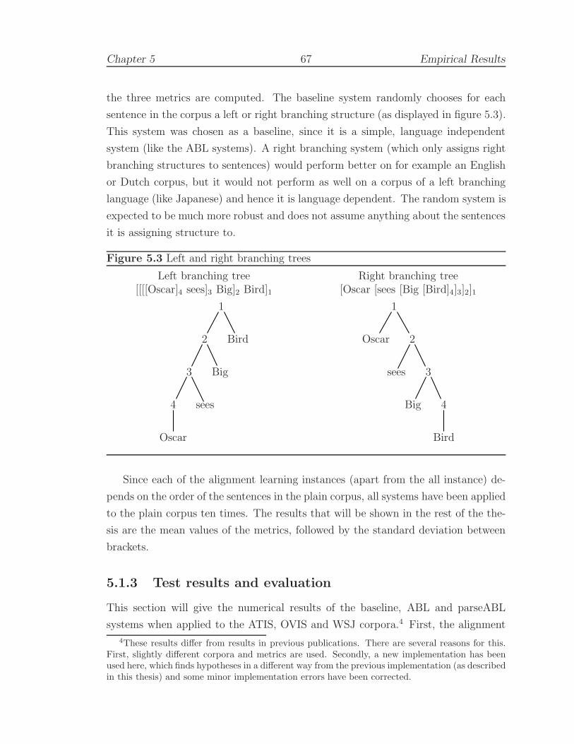
Chapter 5 67 Empirical Results
the three metrics are computed. The baseline system randomly chooses for each
sentence in the corpus a left or right branching structure (as displayed in figure 5.3).
This system was chosen as a baseline, since it is a simple, language independent
system (like the ABL systems). A right branching system (which only assigns right
branching structures to sentences) would perform better on for example an English
or Dutch corpus, but it would not perform as well on a corpus of a left branching
language (like Japanese) and hence it is language dependent. The random system is
expected to be much more robust and does not assume anything about the sentences
it is assigning structure to.
Figure 5.3 Left and right branching trees
Left branching tree[[[[Oscar]4 sees]3 Big]2 Bird]1
1
2
3
4
Oscar
sees
Big
Bird
Right branching tree[Oscar [sees [Big [Bird]4]3]2]1
1
Oscar 2
sees 3
Big 4
Bird
Since each of the alignment learning instances (apart from the all instance) de-
pends on the order of the sentences in the plain corpus, all systems have been applied
to the plain corpus ten times. The results that will be shown in the rest of the the-
sis are the mean values of the metrics, followed by the standard deviation between
brackets.
5.1.3 Test results and evaluation
This section will give the numerical results of the baseline, ABL and parseABL
systems when applied to the ATIS, OVIS and WSJ corpora.4 First, the alignment
4These results differ from results in previous publications. There are several reasons for this.First, slightly different corpora and metrics are used. Secondly, a new implementation has beenused here, which finds hypotheses in a different way from the previous implementation (as describedin this thesis) and some minor implementation errors have been corrected.

Chapter 5 68 Empirical Results
learning phase will be evaluated, followed by the combinations of alignment learn-
ing and selection learning. Finally, after the evaluation on the WSJ corpus, the
parseABL framework will be tested.
5.1.3.1 Alignment learning systems
The alignment learning inserts all hypotheses that will be present in the final tree-
bank (after selection learning). The selection learning phase only removes hypothe-
ses. This means that if constituents in the gold standard cannot be found in the
learned hypothesis space after alignment learning, they will not be present in the
final treebank. The alignment learning phase works best when it inserts as many
correct hypotheses and as few incorrect hypotheses as possible.
To evaluate the alignment learning phase separately from the selection learning
phase, the three alignment learning systems have been applied to the ATIS and
OVIS corpora. This results in ambiguous hypothesis spaces. These hypothesis
spaces cannot be compared to the gold standard directly, since they contain fuzzy
trees instead of proper tree structures.
The hypothesis spaces are evaluated by assuming the perfect selection learning
system. The hypothesis space is disambiguated by selecting only those hypotheses
that are also present in the gold standard. This will give the upper bound on all
metrics. The real selection learning methods (evaluated in the next section) can
never improve on these values.
The results of applying the alignment learning phases to the ATIS and OVIS
corpora and selecting only the hypotheses that are present in the original treebanks
can be found in table 5.1. The precision in this table is 100%, since only correct
constituents are selected from the hypothesis space. The recall indicates how many
of the correct constituents can be found in the learned treebank.
Table 5.2 gives an overview of the number of hypotheses contained in the hy-
pothesis spaces generated by the alignment learning phases. To get an idea of how
these amount compare to the original treebank, the gold standard ATIS and OVIS
treebanks contains respectively 7,197 and 57,661 constituents. Additionally, it shows
how many hypotheses were removed from the hypothesis spaces to build the upper
bound treebanks. The number of constituents present in those treebanks are also
given.
It is interesting to see that the biased system does not perform very well at all.
The recall is low (even compared to the baseline) and the results vary widely as
indicated by the standard deviation. This is the case on both the ATIS and OVIS
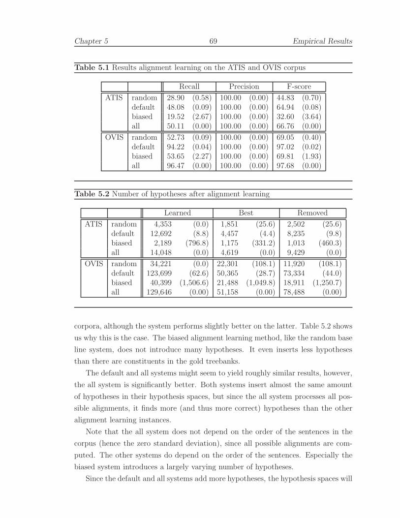
Chapter 5 69 Empirical Results
Table 5.1 Results alignment learning on the ATIS and OVIS corpus
Recall Precision F-score
ATIS random 28.90 (0.58) 100.00 (0.00) 44.83 (0.70)default 48.08 (0.09) 100.00 (0.00) 64.94 (0.08)biased 19.52 (2.67) 100.00 (0.00) 32.60 (3.64)all 50.11 (0.00) 100.00 (0.00) 66.76 (0.00)
OVIS random 52.73 (0.09) 100.00 (0.00) 69.05 (0.40)default 94.22 (0.04) 100.00 (0.00) 97.02 (0.02)biased 53.65 (2.27) 100.00 (0.00) 69.81 (1.93)all 96.47 (0.00) 100.00 (0.00) 97.68 (0.00)
Table 5.2 Number of hypotheses after alignment learning
Learned Best Removed
ATIS random 4,353 (0.0) 1,851 (25.6) 2,502 (25.6)default 12,692 (8.8) 4,457 (4.4) 8,235 (9.8)biased 2,189 (796.8) 1,175 (331.2) 1,013 (460.3)all 14,048 (0.0) 4,619 (0.0) 9,429 (0.0)
OVIS random 34,221 (0.0) 22,301 (108.1) 11,920 (108.1)default 123,699 (62.6) 50,365 (28.7) 73,334 (44.0)biased 40,399 (1,506.6) 21,488 (1,049.8) 18,911 (1,250.7)all 129,646 (0.00) 51,158 (0.00) 78,488 (0.00)
corpora, although the system performs slightly better on the latter. Table 5.2 shows
us why this is the case. The biased alignment learning method, like the random base
line system, does not introduce many hypotheses. It even inserts less hypotheses
than there are constituents in the gold treebanks.
The default and all systems might seem to yield roughly similar results, however,
the all system is significantly better. Both systems insert almost the same amount
of hypotheses in their hypothesis spaces, but since the all system processes all pos-
sible alignments, it finds more (and thus more correct) hypotheses than the other
alignment learning instances.
Note that the all system does not depend on the order of the sentences in the
corpus (hence the zero standard deviation), since all possible alignments are com-
puted. The other systems do depend on the order of the sentences. Especially the
biased system introduces a largely varying number of hypotheses.
Since the default and all systems add more hypotheses, the hypothesis spaces will

Chapter 5 70 Empirical Results
contain more correct hypotheses (as indicated by the higher recall for both systems),
but the selection learning phase also has a harder task, since it has more hypotheses
to choose from. This phase will be investigated next.
5.1.3.2 Selection learning systems
For the evaluation of the complete ABL systems, all instances have been applied
to the two corpora. The recall, precision and f-scores of the ABL systems and the
baseline can be found in table 5.3 for the ATIS corpus and in table 5.4 for the OVIS
corpus.
Remember that the selection learning phase works best when it removes as many
incorrect and as few correct hypotheses from the hypothesis space. If there are many
correct and few incorrect hypotheses in the hypothesis universe, then the selection
learning phase has an easy task selecting the correct hypotheses. From this, it
can be expected that the results of the selection learning phases on the hypothesis
space generated by the biased system will be close to the upper bound, whereas the
selection learning on the hypothesis space of the all system will perform less than
perfect.
Table 5.3 Results selection learning on the ATIS corpus
Recall Precision F-score
random 28.90 (0.58) 33.73 (0.68) 31.13 (0.63)default upper 48.08 (0.09) 100.00 (0.00) 64.94 (0.08)
incr 31.64 (0.94) 38.94 (1.32) 34.91 (1.10)leaf+ 25.82 (0.19) 54.73 (0.42) 35.09 (0.25)branch+ 20.81 (0.20) 46.57 (0.39) 28.76 (0.26)
biased upper 19.52 (2.67) 100.00 (0.00) 32.60 (3.64)incr 18.20 (2.06) 55.32 (4.82) 27.21 (1.59)leaf+ 18.01 (1.39) 56.56 (3.97) 27.23 (1.13)branch+ 17.82 (1.24) 56.62 (3.67) 27.02 (1.03)
all upper 50.11 (0.00) 100.00 (0.00) 66.76 (0.00)incr 32.42 (1.02) 39.34 (1.34) 35.54 (1.16)leaf+ 25.19 (0.11) 53.31 (0.24) 34.21 (0.15)branch+ 20.68 (0.02) 45.25 (0.05) 28.39 (0.03)
Table 5.3 and 5.4 give the results of applying the alignment learning and selection
learning phases to the ATIS and OVIS corpora, respectively. The “upper” selection
learning method corresponds to the results of the previous section, denoting the
upper bound of the results after the selection learning phase.
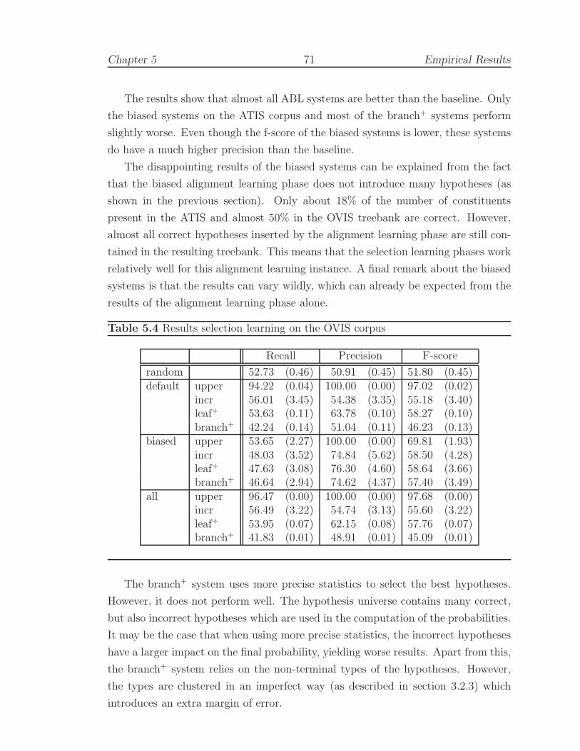
Chapter 5 71 Empirical Results
The results show that almost all ABL systems are better than the baseline. Only
the biased systems on the ATIS corpus and most of the branch+ systems perform
slightly worse. Even though the f-score of the biased systems is lower, these systems
do have a much higher precision than the baseline.
The disappointing results of the biased systems can be explained from the fact
that the biased alignment learning phase does not introduce many hypotheses (as
shown in the previous section). Only about 18% of the number of constituents
present in the ATIS and almost 50% in the OVIS treebank are correct. However,
almost all correct hypotheses inserted by the alignment learning phase are still con-
tained in the resulting treebank. This means that the selection learning phases work
relatively well for this alignment learning instance. A final remark about the biased
systems is that the results can vary wildly, which can already be expected from the
results of the alignment learning phase alone.
Table 5.4 Results selection learning on the OVIS corpus
Recall Precision F-score
random 52.73 (0.46) 50.91 (0.45) 51.80 (0.45)default upper 94.22 (0.04) 100.00 (0.00) 97.02 (0.02)
incr 56.01 (3.45) 54.38 (3.35) 55.18 (3.40)leaf+ 53.63 (0.11) 63.78 (0.10) 58.27 (0.10)branch+ 42.24 (0.14) 51.04 (0.11) 46.23 (0.13)
biased upper 53.65 (2.27) 100.00 (0.00) 69.81 (1.93)incr 48.03 (3.52) 74.84 (5.62) 58.50 (4.28)leaf+ 47.63 (3.08) 76.30 (4.60) 58.64 (3.66)branch+ 46.64 (2.94) 74.62 (4.37) 57.40 (3.49)
all upper 96.47 (0.00) 100.00 (0.00) 97.68 (0.00)incr 56.49 (3.22) 54.74 (3.13) 55.60 (3.22)leaf+ 53.95 (0.07) 62.15 (0.08) 57.76 (0.07)branch+ 41.83 (0.01) 48.91 (0.01) 45.09 (0.01)
The branch+ system uses more precise statistics to select the best hypotheses.
However, it does not perform well. The hypothesis universe contains many correct,
but also incorrect hypotheses which are used in the computation of the probabilities.
It may be the case that when using more precise statistics, the incorrect hypotheses
have a larger impact on the final probability, yielding worse results. Apart from this,
the branch+ system relies on the non-terminal types of the hypotheses. However,
the types are clustered in an imperfect way (as described in section 3.2.3) which
introduces an extra margin of error.

Chapter 5 72 Empirical Results
The incr systems all perform relatively well. The all:incr system even outper-
forms all other systems on the ATIS corpus. From the relatively large standard
deviation of these systems, it can be concluded that the order of the sentences in
the corpora is important.
The default and all systems seem to perform relatively similar, but the leaf+ and
branch+ systems yield significantly better results when combined with the default
system on both corpora. Overall, the default systems perform best. They have high
scores and small standard deviations. From the systems within default, the leaf+
system clearly performs best. For the rest of this chapter, i.e. the results on the
WSJ corpus, the learning curve and parseABL, this system will be used.
5.1.3.3 Results on the Wall Street Journal corpus
To test how the system performs on a completely new corpus, it has been applied to
the Wall Street Journal (WSJ) corpus. This corpus is, like the ATIS corpus, part of
the Penn treebank 2. The default:leaf+ system has been applied to section 23 of this
treebank5, which contains 1,094 sentences. The WSJ corpus consists of newspaper
articles, which means that the sentences are more complex than the ATIS or OVIS
corpora. The main difference between the corpora is that the WSJ corpus has a
much larger vocabulary size. Where the other two corpora are samples of a small
domain, the WSJ corpus is from a much larger domain. Apart from that, the mean
sentence length is over 35 words per sentence. Some example sentences can be found
in 32.
(32) a. At about 3:30 pm EDT S&P futures resumed trading and for a brief time
the futures and stock markets started to come back in line
b. In the year quarter the designer and operator of cogeneration and waste
heat recovery plants had net income of $ 326,000 or four cents a share on
revenue of about $ 414 million
c. Under terms of the plan independent generators would be able to compete
for 15 % of customers until 1994 and for another 10 % between 1994 and
1998
5Section 23 has informally developed into the test section of the WSJ corpus (see e.g. (Collins,1997; Charniak, 1997)).

Chapter 5 73 Empirical Results
Table 5.5 Results ABL on the WSJ corpus
Recall Precision F-score
random 23.94 (0.29) 22.62 (0.27) 23.27 (0.28)upper 52.86 (0.03) 100.00 (0.00) 69.16 (0.03)default:leaf+ 12.46 (0.54) 42.56 (1.73) 19.26 (0.52)
Before looking at the results, it must be mentioned that to our knowledge, this
is the first time an unsupervised language learning system has been applied to the
plain sentences of the Wall Street Journal corpus.
The results of applying the random baseline system, the upper bound of the
alignment learning phase and the default:leaf+ system to section 23 of the WSJ
corpus are shown in table 5.5. The baseline system outperforms the ABL system.
However, default:leaf+ has a much higher precision. Note that applying the sys-
tem to several sections indicate that the recall decreases slightly, but the precision
improves even more.
The upper bound shows that many of the correct hypotheses are being learned.
The selection learning phase, however, is unable to select them. It may be the case
that the leaf+ selection learning system does not perform very well when confronted
with more hypotheses compared to the ATIS and OVIS corpora. Future work should
concentrate on better selection learning methods. Since there are many hypotheses,
the probabilities used in the leaf+ system may not be precise enough. The branch+
system or the systems described in section 7.4 may perhaps perform better (even
though they are based on imprecise non-terminal type data).
5.1.3.4 parseABL systems
For the evaluation of the parseABL system, a grammar has been extracted from
each of the treebanks generated by the default:leaf+ system. Each of the grammars
have been used to parse the plain sentences of the ATIS corpus.6 The results of the
parsed treebanks are shown in table 5.6. The first entry is computed by extracting
an SCFG and the final entry contains the results of the unparsed treebank (as shown
in table 5.3. The other entries show the results of parsing the sentences using STSGs
with the designated maximum tree depth.
6The corpus has been parsed using the efficient DOPDIS parser by Khalil Sima’an (1999). Onlyone minor problem was that the ABL systems sometimes learn too “flat” structure (i.e. constituentscontaining too many elements). The parser has not been optimised for this type of structure.

Chapter 5 74 Empirical Results
Table 5.6 Results parseABL on the ATIS corpus
Treedepth Recall Precision F-score
1 24.87 (0.54) 56.79 (1.00) 34.59 (0.69)2 25.62 (0.17) 55.38 (0.49) 35.03 (0.25)3 25.79 (0.19) 54.74 (0.43) 35.06 (0.26)- 25.82 (0.19) 54.73 (0.42) 35.09 (0.25)
Each of the reparsed corpora have a lower recall, but a higher precision. When
the maximum tree depth is increased, the results grow closer to the unparsed tree-
bank. Since the DOP system has a preference for shorter derivations and thus has a
preference for the use of larger subtrees (Bod, 2000), the STSG instances that have
a higher maximum tree depth will prefer the larger parts of the structures. This
corresponds to the structures that are present in the unparsed treebank generated
by the default:leaf+ system. Increasing the treedepth even more will probably yield
results similar to those of depth 3 and to the unparsed treebank.
5.1.3.5 Learning curve
To investigate how the ABL system responds to differences in amount of input data,
the default:leaf system is applied to corpora of increasing size. The results on the
ATIS corpus can be found in figure 5.4 and those on the OVIS corpus in figure 5.5.
The measures on both corpora seem to have been stabilised when the entire
corpus is used to learn. It might still be the case that if the corpora were larger, the
results would increase slightly, but no drastic improvements are to be expected.
It is interesting to see that the recall and precision metrics both respond similar
to changes. The jump in performance that occurs between sentences 500 and 750 on
the OVIS corpus can be found in all metrics. This shows that the ABL systems is
very balanced. Note that the default:leaf+ system has been applied to the corpora
of different size only once in this section. The large increase in performance is
explained by a number of “easy” sentences in that range. The standard deviation of
the results become smaller when more data is available. When the system is applied
ten times (and using the mean as values), this jump in performance is flattened out.
The system takes a longer time to stabilise on the OVIS corpus than on the
ATIS corpus. The OVIS corpus contains mainly short sentences. These sentences
are easy to structure, since there are not many possible hypotheses to insert. The
ATIS corpus, on the other hand, has longer sentences, which are all about as difficult

Chapter 5 75 Empirical Results
Figure 5.4 Learning curve on the ATIS corpus
100 200 300 400 500
2030
4050
Corpus size
Per
cent
age
RecallPrecisionF−score
to structure. When longer sentences occur early in the corpus, the results on the
OVIS corpus will fluctuate (as happens between sentences 500 and 750). If the longer
sentences occur later in the corpus (for example when the order of the sentences is
different), then there is already enough data in the hypothesis space to absorb the
fluctuation.
5.2 Qualitative results
Apart from the numerical analysis, the treebanks resulting from applying the ABL
systems are analysed and they exhibit some nice properties. This section takes a
closer look at the properties of the generated treebanks. First, a rough “looks-good-
to-me” approach is taken to evaluate the learned treebanks. Following this, it will
be shown that the generated treebanks contain recursive structures.

Chapter 5 76 Empirical Results
Figure 5.5 Learning curve on the OVIS corpus
0 2000 4000 6000 8000 10000
4550
5560
65
Corpus size
Per
cent
age
RecallPrecisionF−score
5.2.1 Syntactic constructions
The learned treebanks all contain interesting syntactic structure. In this section,
three different constructions worth mentioning are discussed. Of course, the struc-
tured corpora contain more, interesting, syntactic constructions, but these three are
most remarkable.
The examples given in this section are taken from a version of the ATIS cor-
pus, which is structured by the default:leaf+ system. The exact non-terminal types
change for each instantiation, but similar constructions can be found in each of the
structured corpora.
Noun phrases The system is able to consistently learn constituents that are similar
to noun phrases. The sentences in 33 show some examples.
(33) a. [How much would the [coach fare cost]1]0
b. [I need a [flight]213 from Indianapolis to Houston on T W A]0
c. [List all [flights]1026 from Burbank to Denver]0

Chapter 5 77 Empirical Results
The ABL system finds almost all noun phrases in the corpus. However, it
inserts constituents that contain the entire noun phrase except for the deter-
miner. This happens because the determiners occur frequently, which means
that they are often linked. When the determiners are linked, the parts of the
sentences following (and preceding) the determiner are stored in a hypothesis.
Note that since the determiners are not inside the noun phrase constituent,
almost all noun phrases are learned incorrectly. Only noun phrases that do not
have a determiner at all or noun phrases containing a noun only are learned
correctly.
From-to phrases A case that is related to the noun phrase constituents is that
of from and to phrases. Since the corpus contains air traffic information,
from and to are words that occur frequently. Like in the previous case, where
determiners are used as a hypothesis boundary, from and to are also linked
regularly. This results in constituents (which are mostly names of places) as
shown in the sentences in 34. It implies that all names of places are found
correctly.
(34) a. [What are the flights from [Milwaukee]54 to [Tampa]55]0
b. [Show me the flights from [Newark]54 to [Los Angeles]55]0
c. [I would like to travel from [Indianapolis]54 to [Houston]55]0
It is interesting to see that even the non-terminal types of the two constituents
are consistent. A from-phrase has type 54 and a to-phrase has type 55.
Part-of-speech tags Apart from the larger constituents described above, ABL
finds many part-of-speech tags of for example verbs, nouns. Many verbs are
clustered into the same non-terminal type. All forms of the verb “to be”
occuring in the corpus are grouped together, but also verbs that occur on
the first position in the sentence have mostly the same type. Additionally,
frequently occuring nouns, like flight, flights, number and dinner have the
same non-terminal types consistently.
5.2.2 Recursion
All tested treebanks structured by the ABL systems contain recursive structure.
This section will concentrate on examples taken from the structured ATIS corpus.
To be completely clear about what recursion is, it is defined here as follows.

Chapter 5 78 Empirical Results
Definition 5.1 (Recursion in a tree)
A (fuzzy) tree T = 〈S, C〉 contains recursive structure iff there are constituents
c1 = 〈b1, e1, n1〉 and c2 = 〈b2, e2, n2〉 ∈ C for which it holds that n1 = n2 and
either (b1 ≤ b2 ∧ e1 ≥ e2) or (b1 ≥ b2 ∧ e1 ≤ e2).
Definition 5.2 (Recursion in a treebank or structured corpus)
A treebank or structured corpus is said to contain recursive structure iff at least one
tree or fuzzy tree contains recursive structure.
The sentences 35, 36, and 37 are examples of recursion in trees found in the ATIS
corpus. The first sentence of the pair is the learned tree, while the second is the
original tree structure. These particular structures can be found in the corpus gen-
erated by the default:leaf+ system, but the other systems learn equivalent recursive
structures.
(35) a. [Fares less than one [hundred fifty one [dollars]32]32]0
b. [Fares less than [[one hundred fifty one]QP dollars]NP]FRAG
In the sentences in 35, the original tree structure did not show any recursion. The
recursive structure, however, can be easily explained. If the sentence is aligned with
for example the sentence Cheapest fare one way, the word one can aligned against
the first or second occurrence. This introduces the structure as shown, although
the non-terminal types may still be different. At some later point, the different
non-terminal types are merged and the recursive structure is a fact.
(36) a. [Is there a flight tomorrow morning from Columbus to [to [Nashville]55]55]0
b. [Is there a flight tomorrow morning from Columbus [to ]X [to Nashville]PP]SQ
The sentences in 36 are a bit strange. The input corpus contained an error, and
this allows different links of the word to, the system learned recursion. Again, the
original corpus did not show any recursion.
(37) a. [Is dinner served on the [first leg or the [second leg]1]1]0
b. [Is dinner served on [[the first leg]NP or [the second leg]NP]NP]SQ
The learned tree structure in the final example, which can be found in 37, is
much more like the original structure. In fact, the constituents would have been
Chapter 5 79 Empirical Results
completely correct if only the determiner was put inside the constituents. The fact
why this is not the case has been discussed in the previous section.
Intuitively, a recursive structure is formed first by building the constituents that
form the structure of the recursion as hypotheses with different root non-terminals.
Now the non-terminals need to be merged. This happens when two partially struc-
tured sentences are compared to each other yielding hypotheses that already existed
in both sentences with the non-terminals present in the “recursive” structure (as
described in sections 3.2.2 and 3.2.3). The non-terminals are then merged, resulting
in a recursive structure.
Chapter 6
ABL versus the WorldThis world is spinning around me.
— Dream Theater (Images and Words)
The general framework has been described and tested in the previous chapters,
so now it can be compared against other systems. This chapter will relate ABL
to other learning systems. In addition, similarities between the ABL and Data-
Oriented Parsing frameworks will be discussed.
This chapter first describes the previous work, giving ABL a niche in the world of
language learning systems. Following this, ABL is compared against other language
learning systems. Next, ABL is extensively compared to the EMILE system, since
EMILE is in many ways similar to ABL and finally, the relationships between ABL
and the DOP framework will be discussed. Even though DOP is not a language
learning system, they have many similarities.
6.1 Background
Before going into a discussion of language learning systems, it must be mentioned
that there is a whole research area dedicated to a formal description of the learn-
ability of languages. Lee (1996) gives a nice overview of this field.
One of the negative results in the theoretical field of language learning is that
by Gold (1967) which proved that learning context-free grammars from text (only)
80

Chapter 6 81 ABL versus the World
is in general impossible.1 Another result, which is even more important in our case,
is by Horning (1969), who showed that stochastic context-free grammars are indeed
learnable. On the other hand, Gold’s concept of identification in the limit has been
amended with the notion of PAC (Probably Approximately Correct) and PACS
(PAC learning under Simple distributions) learning (Valiant, 1984; Li and Vitanyi,
1991). The idea with PAC learning is to minimise the chance of learning something
wrong, without being completely sure to be right.
Existing (language) learning algorithms can be roughly divided into two groups,
supervised and unsupervised learning algorithms, based on the type of information
they use. All learning algorithms use a teacher that gives examples of (unstructured)
sentences in the language. In addition, some algorithms use a critic (also called an
oracle). A critic may be asked if a certain sentence (possibly including structure) is a
valid sentence in the language. The algorithm can use a critic to validate hypotheses
about the language.2 Supervised language learning methods use a teacher and a
critic, whereas the unsupervised methods only use a teacher (Powers, 1997).
Apart from the division of learning systems based on their information, systems
can also be separated based on the types of data they use. Some systems learn
using positive data only, whereas other methods use complete information (positive
as well as negative).
Figure 6.1 shows the different types of language learning systems based on the
type of information and type of data used. The ABL framework falls in the type
4 class, since it is unsupervised (it does not use a critic) and it uses only positive
information (ABL is fed with sentences that can be generated by the language only).
Figure 6.1 Ontology of learning systems
Type of informationSupervised Unsupervised
Type of Complete Type 1 Type 2data Positive Type 3 Type 4
Supervised language learning methods typically generate better results. These
methods can tune their output, since they receive knowledge of the structure of the
language (by initialisation or querying a critic). In contrast, unsupervised language
1Although the learning of context-free grammars in general is not possible, Gold’s theorems donot cover all cases, such as for example finite grammars (Adriaans, 1992, pp. 43–44).
2When an algorithm uses a treebank or structured corpus to initialise, it is said to be supervised.The structure of the sentences in the corpus can be seen as the critic.

Chapter 6 82 ABL versus the World
learning methods do not receive these structured sentences, so they do not know at
all what the output should look like and therefore cannot adjust the output towards
the “expected” output.
Although unsupervised methods perform worse than supervised methods, un-
supervised methods are necessary for the (otherwise) time-consuming and costly
creation of treebanks of languages for which no initial treebank nor grammar yet
exists. This indicates that there is a strong practical motivation to develop unsu-
pervised grammar induction algorithms that work on plain text.
6.2 Bird’s-eye view over the world
This section will briefly describe some of the existing language learning systems.
First, systems using complete information (types 1 and 2) will be described. Next,
the systems which use positive information only will be considered, subdividing these
into supervised (type 3) and unsupervised (type 4).
When progressing the next sections, more detail will be given towards types and
systems that are more closely related to ABL, but even the section on unsupervised
systems using only positive information is not meant to be a complete overview of
the (sub-)field. These short descriptions are merely given to illustrate the ideas of
the established work in this area.
6.2.1 Systems using complete information
For completeness sake, this section will describe two systems that use positive as
well as negative examples to learn a grammar. First, a supervised system which
uses partially structured sentences will be described, followed by an unsupervised
system.
Sakakibara and Muramatsu (2000) describe a system that induces a grammar
using partially structured sentences. The partially structured sentences are stored
in a tabular representation (similar to the one used in the CYK algorithm (Younger,
1967)). A genetic algorithm partitions the set of non-terminals, effectively merging
certain non-terminals. The different possible partitions are then tested against the
negative examples.
The system by Nakamura and Ishiwata (2000) learns a context-free grammar
from positive and negative examples by adapting the CYK algorithm, which intro-
duces a grammar rule if the sentence is otherwise not parsable. If the introduction

Chapter 6 83 ABL versus the World
of a grammar rule allows for parsing a negative example, the system returns failure.
This approach is in a way similar to the alignment learning phase of ABL. Parts of
sentences that cannot be parsed (which are parts that are unequal to the right-hand
side of the known grammar rules) are used to introduce hypotheses. However, no
disambiguation takes place, the system returns failure when overlapping hypotheses
are introduced (in contrast to ABL which has selection learning as a disambiguation
phase).
Both systems are evaluated by letting the system rebuild a known context-free
grammar. The emphasis of the first system, however, is on how many iterations
of the genetic algorithm are needed to find a grammar similar to the original one,
whereas the second system concentrates on processing time needed to find the gram-
mar. This approach unfortunately makes it impossible to compare the two systems
directly. Furthermore, it is unclear how the two methods would perform on real
natural language data.
6.2.2 Systems using positive information
The systems described in this section (which use positive examples only) are more
closely related to the ABL system than the systems in the previous section. First,
some supervised systems will be described, followed by a section on unsupervised
systems.
The section on unsupervised systems also contains some systems that learn word
categories or segment sentences only. Even though these systems are different from
ABL in that ABL learns context-free grammars, they are treated here because they
start with similar information and are in some ways similar to ABL.
6.2.2.1 Supervised systems
The supervised Transformation-Based Learning system described in (Brill, 1993),
is a non-probabilistic system. It starts with naive knowledge on structured sen-
tences (for example right branching structures). The system then compares these
structured sentences against the correctly structured examples. From the differ-
ences between the two, the system learns “transformations”, which can transform
the naive structure into the correct structure. The learned transformations can then
be used to correctly structure new (unstructured) text, by first assuming the naive
structure and then applying the transformations. The system is evaluated by apply-
ing it to the Wall Street Journal treebank, which yields very good results. However,

Chapter 6 84 ABL versus the World
the initial structure of the sentences is taken to be right branching, which is already
quite similar to the structure of English sentences. This means that not many trans-
formations are needed to convert it into the correct structure. It is unclear how well
this method would work on a corpus of a mainly left branching language.
The ALLiS system (Dejean, 2000) is based on theory refinement. It starts by
building a roughly correct grammar based on background knowledge. This initial
grammar is extracted from structured examples. When the grammar is confronted to
the bracketed corpus, revision points in the grammar are found. For these revision
points, possible revisions are created. The best of these is chosen to revise the
grammar. This is repeated until no more revision points are found. Like the previous
system, this method is evaluated on a natural language treebank (although it is not
mentioned which treebank is used). The evaluation concentrates on the structure
of noun phrases and verb phrases only, therefore, it is unclear how well this method
can generate structure for complete sentences.
In his thesis, Osborne (1994) builds a grammar learning system by combining
a model-driven with a data-driven approach. The model-driven system starts with
a grammar and meta-rules which describe how to introduce new grammar rules.
The data-driven system extracts counts from a structured corpus and uses these
counts to prune the new rules induced by the meta-rules. The system is extensively
tested on a treebank, measuring several different metrics. These tests show that the
combination of data-driven and model-driven approach performs best. However, it
is unclear how the quality of the initial grammar, needed for the model-driven part
of the system, influences the results of the entire system.
Pereira and Schabes (1992) describe a system that uses a partially bracketed
corpus to infer parameters of a Stochastic Context-Free Grammar (SCFG) using
inside-outside reestimation. It is tested by letting the system rebuild a grammar
(one that generates palindrome sentences) and by applying it to the ATIS corpus
(which is a different version of the one that is used in this thesis). It is possible to use
this system on a raw (unbracketed) corpus, but the results decrease drastically. Hwa
(1999) uses a variant of Pereira and Schabes system in which the inferred grammars
are represented in a different formalism, which is slightly more efficient. This version
is again tested on the ATIS (and, additionally, on the Wall Street Journal) corpus,
however, the system is pre-trained on 3600 fully structured sentences from the Wall
Street Journal treebank.
The algorithm described by Sakakibara (1992) is in many ways similar to the
algorithm by Sakakibara and Muramatsu (2000), which uses complete data. Again,

Chapter 6 85 ABL versus the World
structured examples are used to initialise the grammar, but instead of using negative
information to decide which partitions can be used to merge non-terminals, the algo-
rithm merges non-terminals to make the grammar reversible.3 Nevado et al. (2000)
describe a version of the Sakakibara algorithm generating a stochastic context-free
grammar. This method has been tested on a subset of the Wall Street Journal tree-
bank, but the only metrics mentioned are the number of iterations the algorithm
needed, the number of learned grammar rules and the perplexity of the learned
grammar.
6.2.2.2 Unsupervised systems
Before discussing unsupervised grammar induction systems, a brief overview of sys-
tems that learn syntactic categories will be given. Next, an article which describes
systems that find word boundaries is mentioned. Finally, unsupervised grammar
induction systems using positive data only will be treated.
Huckle (1995) gives a brief overview of systems that cluster (semantically) similar
words based on the distribution of the contexts of the words and their psychological
relevance. His system uses a Naive Bayes method (Duda and Hart, 1973), which for
each word, counts occurrences of words in the contexts of the considered word. The
distance between two words is computed by taking into account the counts of the
words in the different contexts. However, the evaluation of the systems, using the
looks-good-to-me approach, is meager.
The system described in (Finch and Chater, 1992) bootstraps a set of categories.
Words in the input text are classified in the same category when they can be replaced
in the same contexts (i.e. according to a similarity measure). It is based on bigram
statistics describing the contexts of the words. This system can also be used to
classify short sequences of words. The article by Redington et al. (1998) contains
the results of several experiments of a similar system that classifies words using
distributional information. A system based on neural networks can be found in
(Honkela et al., 1995). Using a Self-Organising Map (SOM) the words of the input
text are roughly clustered according to their semantic type. All articles evaluate
their system using the looks-good-to-me approach, which makes it impossible to
compare them directly. Additionally, the article by Redington et al. makes a more
3A grammar is called reversible if:
1. it is invertible, that is, A → α and B → α implies A = B, and
2. it is reset-free, that is, A → αBβ and A → αCβ implies B = C.

Chapter 6 86 ABL versus the World
formal evaluation by computing accuracy, completeness and informativeness.
The ABL framework is in some ways a generalisation of the systems described
above. Where these systems take a fixed window size for the context of a word or
word sequence, ABL considers the entire sentence as context. If there is some context
that can be found in at least two sentences, ABL will introduce the hypotheses of
the words within that context, i.e. the unequal parts. This allows ABL to learn
constituents of any size.
Brent (1999) describes the comparison of a variety of systems (by other people)
that segment sentences finding word boundaries (which were not present in the input
data). The systems do not generate grammars, but some structure (in the form of
word boundaries) is found. The system is evaluated on the CHILDES corpus, which
contains phonemic transcriptions of child-directed English, by computing recall and
precision metrics. This system does not learn any further syntactic structure, it is
only evaluated on how well it finds word boundaries.
Algorithms that use the minimum description length (MDL) principle build
grammars that describe the input sentences using the minimal number of bits. The
MDL principle results in grouping re-occurring parts of sentences yielding a reduc-
tion in the amount of information needed to describe the corpus. The system by
Grunwald (1994) makes use of the MDL principle. Similarly, de Marcken (1995,
1996, 1999) uses the MDL principle to find structure in (unsegmented) text. This
system finds word boundaries and inner-word structure. Most of these articles only
perform a looks-good-to-me evaluation. Only de Marcken (1996) does a more for-
mal evaluation. The recall and crossing-brackets rate is computed. Unfortunately,
it uses other corpora than the Brent (1999) article, which again makes it impossible
to compare the systems.
The ABL system does not make use of the MDL principle, but by introducing
hypotheses, it indicates how the plain sentences can be compressed (as shown in
figure 2.3 on page 12). By taking the unequal parts of sentences as hypotheses it
compresses the input sentences better than when using the equal parts of sentences
as hypotheses.
Stolcke (1994) and Stolcke and Omohundro (1994) describe a grammar induction
method that merges elements of models using a Bayesian framework. At first, a
simple model is generated (typically, just the set of examples). These examples are
then chunked (i.e. examples are split into sub-elements). By merging the elements of
this set, more complex models arise. Elements are merged guided by the Bayesian
posterior probability (which indicates when the resulting grammar is “simpler”).

Chapter 6 87 ABL versus the World
Evaluation is again done by rebuilding a grammar. In the ABL framework, non-
terminals are merged in the clustering step as described in section 3.2.3 on page 31.
Future extensions may take an approach similar to the one described in these articles
(see section 7.3 on page 101).
Chen (1995) presents a Bayesian grammar induction method, which is followed
by a post-pass using the inside-outside algorithm (Lari and Young, 1990). The
system starts with a grammar that generates left-branching tree structures. The
grammar rules are then changed and the probability of the resulting grammar based
on the observations (example sentences) is computed, where smaller grammars are
favoured over larger ones. Afterwards, the grammar is rebuilt using the inside-
outside algorithm. This method is tested on the part-of-speech tags of the WSJ
corpus, where the entropy of the resulting grammar is used as the evaluation metric.
Similarly, Cook et al. (1976) describe a hill-climbing algorithm (which chooses
another grammar if the cost of that grammar is better than the cost of the current
grammar). The cost function “measures the complexity of a grammar, as well as
the discrepancy between its language and a given stochastic language sample.” The
method is evaluated by letting the system rebuild some simple context-free grammars
and examining the result using the looks-good-to-me approach.
The system by Wolff has a long history in the field of language learning. His
earlier work describes a sentence segmentation system called MK10 (Wolff, 1975,
1977). It computes the joint frequencies of contiguous elements in the sentence.
When a pair of elements occurs regularly, it is taken to be an element itself. Later
work (Wolff, 1980, 1982, 1988) describes SNPR, which is more directed towards
finding context-free grammars describing the example sentences. The system is
explained from the viewpoint of compression (Wolff, 1996, 1998a,b). Again, the
systems are evaluated using a looks-good-to-me approach.
Sequitur is a system developed by Nevill-Manning and Witten (1997) and is in
many ways related to the SNPR system. It generates a grammar by incrementally
inserting the words of the sample sentences in the grammar. Sequitur then makes
sure that the following constraints are always satisfied: digram uniqueness, which
means that no pair of adjacent symbols (words) appears more than once in the
grammar and rule utility, which makes sure that every rule is used more than once.
An interesting feature of this system is that it runs in linear time and space. The
system is mostly evaluated on a formal basis (in the form of time and space com-
plexity). Other than that, it has been applied to several corpora, but only some
features of the learned structure are discussed (very briefly).

Chapter 6 88 ABL versus the World
Magerman and Marcus (1990) describe a method that finds constituent bound-
aries (called distituents) using mutual information values of the part of speech
n-grams within a sentence. The mutual information describes which words cannot
be adjacent within a constituent. Between these words there should be a constituent
boundary. The evaluation of this system is vague. It has been applied to a corpus,
but the results are only given as rough mean error rates.
The system by Clark (2001b) combines several techniques. First of all, it uses
distributional clustering to find grammar rules. A mutual information criterion is
then used to remove incorrect non-terminals. These ideas are incorporated into a
MDL algorithm. The system has been evaluated similarly to the evaluation of the
ABL system in this thesis, even using the same corpus and evaluation metrics. The
main difference with ABL, however, is that Clark’s system has been trained on the
large British National Corpus before applying it to the ATIS corpus. Furthermore,
the system is tested on part-of-speech tags instead of the plain words.
Klein and Manning (2001) describe two systems: the Greedy-Merge system
clusters part-of-speech tags according to a cost (divergence) function, whereas the
Constituency-Parser “learns distributions over sequences representing the probabil-
ity that a constituent is realized as that sequence.” The exact details of the systems
are hard to understand from the article, but both systems are evaluated on the
part-of-speech tags of the Wall Street Journal corpus. This allows it to be roughly
compared against the system by Clark.
From the description of the systems it may be clear that it is nearly impossible
to compare two systems. The systems are divided over the three ways of evaluation
(as described in section 5.1.1), but even the systems that evaluate using the same
approach as in this thesis are nearly impossible to compare, since other (subsets of)
corpora, grammars or metrics are used.
The evaluation of methods described by Clark (2001b), Klein and Manning
(2001) and Pereira and Schabes (1992) comes reasonably close to ours. Pereira and
Schabes (1992) use a slightly different version of the ATIS corpus. Clark (2001b)
trains his system on the BNC corpus. Unlike the ABL system, all systems (includ-
ing the one by Klein and Manning (2001)) use sequences of part-of-speech tags as
sentences.
Now several grammar induction systems have been discussed briefly, we will take
a more detailed look at the EMILE system, since it is the system most similar to
ABL. Most of the next section has been previously published in van Zaanen and
Adriaans (2001a,b).

Chapter 6 89 ABL versus the World
6.3 Zooming in on EMILE
The EMILE 4.14 algorithm is motivated by the concepts behind categorial grammar
and it falls into the PACS paradigm (Li and Vitanyi, 1991). The theoretical concepts
used in EMILE 4.1 are elaborated on in articles on EMILE 1.0/2.0 (Adriaans, 1992)
and EMILE 3.0 (Adriaans, 1999). More information on the precursors of EMILE
4.1 may be found in the above articles, as well as in Dornenburg’s (1997) Master’s
thesis. The EMILE 4.1 algorithm was designed and implemented by Vervoort (2000).
Adriaans et al. (2000) report some experiments using the EMILE system on large
corpora.
The general idea behind EMILE is the notion of identification of substitution
classes by means of clustering. If a language has a context-free grammar, then ex-
pressions that are generated from the same non-terminal can be substituted for each
other in each context where that non-terminal is a valid constituent. Conversely, if
there is a sufficiently rich sample from this language available, then one expects to
find classes of expressions that cluster together in comparable contexts. Figure 6.2
illustrates how EMILE finds clusters and contexts. The context Oscar likes occurs
with the expressions all dustbins and biscuits. Actually, this type of clustering can
be seen as a form of text compression (Grunwald, 1994).
EMILE’s notion of substitution classes exactly coincides with the notion depicted
in figure 2.4 on page 13, which shows that unequal parts of sentences can easily be
generated from the same non-terminal.
Figure 6.2 Example clustering expressions in EMILE
Sentences Structure
Oscar likes all dustbins 1→Oscar likes 2Oscar likes biscuits 2→all dustbins
2→biscuits
This finding gives rise to the hypothesis (possibly unjustified) that these two
expressions are generated from the same non-terminal. If enough traces of a whole
group of expressions in a whole group of contexts are found, the probability of this
hypothesis grows. In other words, grammar rules are only introduced when enough
4EMILE 4.1 is a successor to EMILE 3.0, conceived by Adriaans. The original acronym standsfor Entity Modelling Intelligent Learning Engine. It refers to earlier versions of EMILE that alsohad semantic capacities. The name EMILE is also motivated by the book on education by J.-J.Rousseau.

Chapter 6 90 ABL versus the World
evidence has been seen and thus only when the probability of the hypothesis is high
enough.
The difference with ABL’s approach is that instead of inserting hypotheses about
constituents in the hypothesis space, the unequal parts of the sentences are clustered
(i.e. grouped) in rewrite rules directly. However, ABL always stores the possible
constituents, whereas EMILE only induces grammar rules when enough evidence
has been found. EMILE never introduces conflicting grammar rules; the grammar
rules with the highest probabilities are stored.
For a sentence of length n the maximal number of different contexts and expres-
sions is 1/2n(n + 1).5 The complexity of a routine that clusters all contexts and
expressions is polynomial in the number of contexts and expressions.
The EMILE family of algorithms works efficiently for the class of shallow context-
free languages with characteristic contexts and expressions provided that the sample
is taken according to a simple distribution (Adriaans, 1999). An expression of a
type T is characteristic for T if it only appears with contexts of type T . Similarly,
a context of a type T is characteristic for T if it only appears with expressions of
type T . In the example one might see the context Oscar likes as characteristic for
noun phrases and the phrases all dustbins and biscuits as characteristic for noun
contexts. If more occurrences of the characteristic contexts and types are found, the
certainty that these are characteristic grows.
A distribution is simple if it is recursively enumerable. A class of languages C
is shallow if for each language L it is possible to find a grammar G, and a set of
sentences S inducing characteristic contexts and expressions for all the types of G,
such that the size of S and the length of the sentences of S are logarithmic in the
descriptive length of L (relative to C). Languages with characteristic contexts and
expressions for each syntactic type are called context- and expression-separable. A
sample is characteristic if it allows us to identify the right clusters that correspond
with non-terminals in the original grammar.
Samples generated by arbitrary probability distributions are very likely to be
non-characteristic. One can prove, however, that if the sample is drawn according
to a simple distribution and the original grammar is shallow then the right clusters
will be found in a sample of polynomial size, i.e. one will have a characteristic sample
of polynomial size.
Natural languages seem to be context- and expression-separable for the most
5Note that EMILE’s cluster routine does a more extensive search for patterns than a k-gramroutine that distinguishes only n− (k − 1) elements in a sentence

Chapter 6 91 ABL versus the World
part, i.e. if there are any types lacking characteristic contexts or expressions,6 these
types are few in number, and rarely used. Furthermore, there is no known example of
a syntactic construction in a natural language that cannot be expressed in a short
sentence. Hence the conjecture that natural languages are (mostly) context- and
expression-separable and shallow seems tenable. This explains why EMILE works
for natural language.
The EMILE 4.1 algorithm consists of two main stages: clustering and rule in-
duction. In the clustering phase all possible contexts and expressions of a sample
are gathered in a matrix. Starting from random seeds, clusters of contexts and
expressions, that form correct sentences, are created.7 If a group of contexts and
expressions cluster together they receive a type label. This creates a set of proto-
rules. In the example, the proto-rules 1 →Oscar likes 2 and 2 → all dustbins can be
found (if there is enough evidence for them). The sentence type 1 can be rewritten
as Oscar likes concatenated to an expression of type 2.
A concise method for rule creation is used in the rule induction phase.8 In the
rule induction phase, sentences in the input are partially parsed using the set of
proto-rules. It introduces new grammar rules by applying the proto-rules. New
rules are derived by substitution of types for characteristic sub-expressions in typed
expressions (Adriaans, 1992). Suppose for instance that the expression all dustbins
is characteristic for type 2. It is then possible to form the rule 3 → cleans 2 with a
brush from the rule 3 → cleans all dustbins with a brush.
In (Adriaans, 1999) it is shown that the EMILE 3.0 algorithm can PACS learn
shallow context-free (or categorial) languages with context- and expression separa-
bility in time polynomial to the size of the grammar. EMILE 4.1 is an efficient
implementation of the main characteristics of 3.0.
6.3.1 Theoretical comparison
While ABL directly (and greedily) structures sentences, EMILE tries to find gram-
mar rules in two steps. It first finds proto-rules and using these proto-rules it in-
troduces new grammar rules. Rules are only introduced when enough evidence has
been found. This duality is actually the main difference of the two systems. Since
ABL considers much more hypotheses, it results in ABL being slower (i.e. taking
6After rewriting types such as ‘verbs that are also nouns’ as composites of basic types.7A set of parameters and thresholds determines the significance and the amount of noise in the
clusters.8EMILE 3.0 uses a much more elaborate, sound rule induction algorithm, but it is impossible
to implement this routine efficiently.

Chapter 6 92 ABL versus the World
more time and thus working on smaller corpora) in contrast to EMILE, which is
developed to work on much larger corpora (say over 100,000 sentences).
The inner working of the algorithms is completely different. EMILE finds a
grammar rule when enough information is found to support the rule. Evidence
for grammar rules is found by searching the matrix, which contains information
on possible contexts and expressions. In other words, EMILE first finds a set of
proto rules. The second phase uses these proto-rules to search for occurrences of
the right-hand side of a proto-rule in the unstructured data, which indicates that
the rule might have been used to generate that sentence. This knowledge is used to
insert new grammar rules.
In contrast, ABL searches for unequal parts of sentences, since these parts might
have been generated from the same non-terminal type (substitution class in EMILE’s
terminology). ABL remembers all possible substitution classes it finds and only
when all sentences have been considered and all hypotheses are found, the “best”
constituents are selected from the found hypotheses.
One more interesting feature worth mentioning is that EMILE (like ABL) can
learn recursive structures.
6.3.2 Numerical comparison
The two systems have been tested on two treebanks: the Air Traffic Information
System (ATIS) treebank and the Openbaar Vervoer Informatie Systeem (OVIS)
treebank. Both treebanks have been described in section 5.1.2.1 on page 62. The
only difference here is that one-word sentences have been removed beforehand. This
explains the slightly different results of ABL in table 6.1.
The same evaluation approach as described in chapter 5 has been used. ABL and
EMILE have both been applied to the plain sentences of the two treebanks. The
structured sentences generated by ABL have been directly compared against the
structured sentences in the original corpus. EMILE builds a context-free grammar.
The plain sentences in the original corpus are parsed using this grammar and the
parsed sentences are compared against the original tree structures.
An overview of the results of both systems on the two treebanks can be found
in table 6.1. The figures in the tables again represent the mean values of the metric
followed by their standard deviations (in brackets). Each result is computed by
applying the system ten times on the input corpus.
Note that the OVIS and ATIS corpora are certainly not characteristic for the

Chapter 6 93 ABL versus the World
Table 6.1 Results of EMILE and ABL
Recall Precision F-score
ATIS EMILE 16.81 (0.69) 51.59 (2.71) 25.35 (1.00)ABL 25.77 (0.22) 54.52 (0.45) 35.00 (0.29)
OVIS EMILE 36.89 (0.77) 49.93 (1.96) 41.43 (3.21)ABL 53.59 (0.07) 63.99 (0.08) 58.33 (0.06)
underlying grammars. It is therefore impossible to learn a perfect grammar for these
corpora from the data in the corpora.9
As can be seen from the results, ABL outperforms EMILE on all metrics on both
treebanks. Since EMILE has been developed to work on large corpora (much larger
than the ATIS and OVIS treebanks), the results are disappointing. However, it
may well be the case that EMILE will outperform the ABL system on such corpora.
ABL is a more greedy learner (it finds as many hypotheses as possible and then
disambiguates the hypothesis space), whereas EMILE is much more cautious. Once
a grammar rule has been inserted in the grammar, it is considered correct.
Another explanation why ABL outperforms EMILE is that the EMILE system
has many parameters which influence for example the greediness of the algorithm.
By adjusting the parameters, a different grammar may be found, which perhaps
performs better than this one. Several settings have been tried and the results
shown seem to be the best. This does not mean that there does not exist a better
setting of the parameters.
Finally, the results of EMILE may be worse than those of ABL, because the sen-
tences had to be parsed with the grammar generated by EMILE. A non-probabilistic
parser is used to generate these results. This may also explain the large standard
deviations in the results. If there are many derivations of the input sentences, the
system will select one at random. Since the structured sentences are all parsed ten
times, other derivations may have been chosen, generating variable results.
6.4 ABL in relation to the other systems
Now that several language learning systems have been described and ABL is more
closely compared against the EMILE system, this section will relate ABL to estab-
9It is our hypothesis that one needs a corpus of at least 50,000,000 sentences to get an acceptablegrammar of the English language on the basis of the EMILE algorithm.
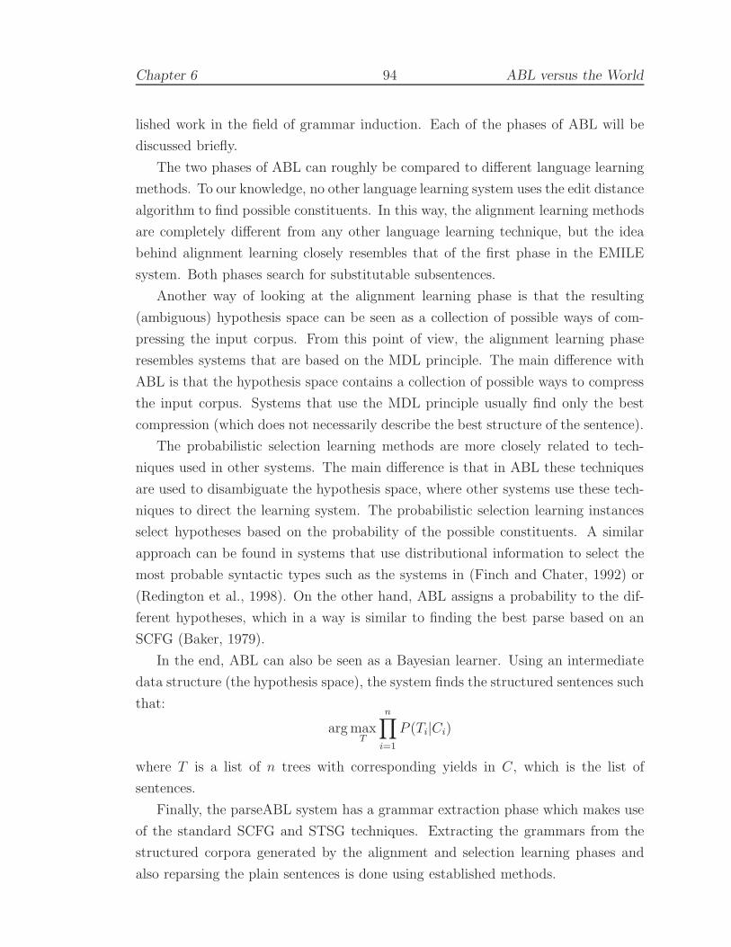
Chapter 6 94 ABL versus the World
lished work in the field of grammar induction. Each of the phases of ABL will be
discussed briefly.
The two phases of ABL can roughly be compared to different language learning
methods. To our knowledge, no other language learning system uses the edit distance
algorithm to find possible constituents. In this way, the alignment learning methods
are completely different from any other language learning technique, but the idea
behind alignment learning closely resembles that of the first phase in the EMILE
system. Both phases search for substitutable subsentences.
Another way of looking at the alignment learning phase is that the resulting
(ambiguous) hypothesis space can be seen as a collection of possible ways of com-
pressing the input corpus. From this point of view, the alignment learning phase
resembles systems that are based on the MDL principle. The main difference with
ABL is that the hypothesis space contains a collection of possible ways to compress
the input corpus. Systems that use the MDL principle usually find only the best
compression (which does not necessarily describe the best structure of the sentence).
The probabilistic selection learning methods are more closely related to tech-
niques used in other systems. The main difference is that in ABL these techniques
are used to disambiguate the hypothesis space, where other systems use these tech-
niques to direct the learning system. The probabilistic selection learning instances
select hypotheses based on the probability of the possible constituents. A similar
approach can be found in systems that use distributional information to select the
most probable syntactic types such as the systems in (Finch and Chater, 1992) or
(Redington et al., 1998). On the other hand, ABL assigns a probability to the dif-
ferent hypotheses, which in a way is similar to finding the best parse based on an
SCFG (Baker, 1979).
In the end, ABL can also be seen as a Bayesian learner. Using an intermediate
data structure (the hypothesis space), the system finds the structured sentences such
that:
argmaxT
n∏
i=1
P (Ti|Ci)
where T is a list of n trees with corresponding yields in C, which is the list of
sentences.
Finally, the parseABL system has a grammar extraction phase which makes use
of the standard SCFG and STSG techniques. Extracting the grammars from the
structured corpora generated by the alignment and selection learning phases and
also reparsing the plain sentences is done using established methods.

Chapter 6 95 ABL versus the World
6.5 Data-Oriented Parsing
This section will relate ABL to the Data-Oriented Parsing (DOP) framework (Bod,
1995, 1998). Large parts of this section can also be found in (van Zaanen, 2002).
Data-Oriented Parsing and Alignment-Based Learning are two completely dif-
ferent systems with different goals. The DOP framework structures sentences based
on known structured past experiences. ABL is a language learning system searching
for structure using unstructured sentences only. However, the global approach both
choose to tackle their respective problems is similar.
Both the DOP and ABL frameworks consist of two phases. The first phase builds
a search space of possible solutions and the second phase searches this space to find
the best solution. In the first phase, DOP considers all possible combinations of
subtrees in the tree grammar that lead to possible derivations of the input sentence.
The second phase then consists of finding the best of these possibilities by computing
the most probable parse, effectively searching the “derivation-space”, which contains
substructures of the sentences.
ABL has a similar setup. The first phase (alignment learning) consists of building
a search space of hypotheses by aligning sentences to each other. The second phase
(selection learning) searches this space (using for example a statistical evaluation
function) to find the best set of hypotheses.
ABL and DOP are similar in remembering all possible solutions in the search
space for further processing later on. The advantage of proceeding in this way is
that the final search space contains more precise (statistical) information. ABL and
DOP make definite choices using this more complete information, in contrast to
systems that choose between mutually exclusive solutions at the time when they are
found.
Note that ABL and DOP do not necessarily compute all solutions, but all (or at
least many) solutions are present in a compact data structure. Taking into account
all solutions is possible by searching this data structure.
6.5.1 Incorporating ABL in DOP
Here we describe two extensions of the DOP system using ABL. One way of ex-
tending DOP is to use ABL as a bootstrapping method generating an initial tree
grammar. The other way is to have ABL running next to DOP to enhance DOP’s
robustness.

Chapter 6 96 ABL versus the World
6.5.1.1 Bootstrapping a tree grammar
One of the main reasons for developing ABL was to allow a parser to work on un-
structured text without knowing the underlying grammar beforehand. From this it
follows directly that ABL can be used to enhance DOP with a method to bootstrap
an initial tree grammar. All DOP methods assume an initial tree grammar con-
taining subtrees. These subtrees are normally extracted from a structured corpus.
However, if no such corpus is available, DOP cannot be used directly.
Normally, a structured corpus is built by hand. However, as described in chap-
ter 2, this is expensive. For each language or domain, a new structured corpus is
needed and manually building such a corpus is not be feasible due to time and cost
restrictions. Automatically building a structured corpus circumvents these prob-
lems. Unstructured corpora are built more easily and applying an unsupervised
grammar bootstrapping system such as ABL to an unstructured corpus is relatively
fast and cheap.
Figure 6.3 gives an overview of the combined ABL and DOP systems. The upper
part describes how ABL is used to build a structured corpus, while the lower part
indicates how DOP is used to parse a sentence. Both systems are used as usual,
the figure merely illustrates how both systems can be combined. Starting out with
an unstructured corpus, ABL bootstraps a structured version of that corpus. From
this, subtrees are extracted using the regular method, which can then be used for
parsing. Note that subtrees extracted from the sentences parsed by DOP can again
be added to the tree grammar.
Figure 6.3 Using ABL to bootstrap a tree grammar for DOP
Plaincorpus
ABL Structuredcorpus
Sentence DOP Treegrammar
Extractsubtrees
Parsed sentence

Chapter 6 97 ABL versus the World
6.5.1.2 Robustness of the parser
The standard DOP model breaks down on sentences with unknown words or un-
known syntactic structures. One way of solving this problem (in contrast to the
DOP models described in (Bod, 1998)) is to let ABL take care of these cases. The
main advantage is that even new syntactic structures (which were not present in the
original tree grammar) can be learned. To our knowledge, no other DOP instantia-
tion does this.
Figure 6.4 shows how, when DOP cannot parse a sentence,10 the unparsable
sentence is passed to ABL. Applying ABL to the sentence results in a structured
version of the sentence. Since this structured sentence resembles a parsed sentence,
it can be the output of the system. Another approach may be taken, where subtrees,
extracted from the sentence structured by ABL, are added to the tree grammar and
DOP will reparse the sentence (which will definitely succeed).
Figure 6.4 Using ABL to adjust the tree grammar
Unparsablesentence
ABL Structuredsentence
Sentence DOP Treegrammar
Extractsubtrees
Parsed sentence
The main problem with this approach is that ABL cannot learn structure using
the unparsable sentence only; ABL always needs other sentences to align to. Ad-
ditionally, for any structure to be found, ABL needs at least two sentences with at
least one word in common. There are several ways to solve this problem.
One way to find sentences for ABL to align is extracting them from the tree
grammar used by DOP. If complete tree structures are present in the tree gram-
mar, the yield of these trees (i.e. the plain sentences) can be used to align to the
unparsable sentence. Furthermore, using the structure present in the trees from the
tree grammar, the correct type labels might be inserted in the unparsable sentence.
10It is assumed that the unparsable sentence is a correct sentence in the language and that thegrammar (in the form of DOP subtrees) is not complete.

Chapter 6 98 ABL versus the World
If no completely lexicalised tree structures representing sentences are present
in the tree grammar (for example, because they have been removed by pruning),
sentences can still be found by generating them from the subtrees. Using a smart
generation algorithm can assure that at least some words in the unparsable sentence
and the generated sentences are the same.
A completely different method of finding plain sentences which ABL can use to
align to is by running ABL parallel to DOP. Each sentence DOP parses (correctly
or incorrectly) is also given to ABL. These sentences can then be used to learn
structure. When sentences are parsed with DOP, ABL builds its own structured
corpus which can be used to align unparsable sentences to.
Additional information about the unparsable sentence can be gathered when
ABL initialises the structure of the unparsable sentence with information from the
(incomplete) chart DOP has built. The incomplete chart contains structure based
on the subtrees in the treebank. These subtrees are a good indication of part of
the structure of the sentence even though the subtrees cannot be combined into a
complete derivation.
6.5.2 Recursive definition
If DOP uses ABL (section 6.5.1) and ABL uses DOP (section 4.3.2 on page 54
and 7.4.2.2 on page 105) at the same time, there seems to be an infinite loop between
the systems, which is impossible to implement. However, when taking a closer look,
DOP is extended with ABL as a bootstrapping method or to improve robustness.
On the other hand, ABL is extended with DOP as an improvement to the stochastic
evaluation function or to reparse sentences. In the latter case, there is no need for
the robuster version of DOP. The DOP system that is used to extend ABL is not the
extended DOP system, so effectively there is no recursive use between both systems.

Chapter 7
Future Work:
Extending the FrameworkHmmm, especially enjoyed that one. . .
Let’s see what’s next. . .
— Offspring (Smash)
This chapter will describe several possible extensions of the standard ABL sys-
tem. At the moment, these extensions have not yet been implemented.
First, three extensions of the alignment learning phase will be described, followed
by two possible extensions of the selection learning phase. Next, two extensions that
influence the entire system are discussed, and finally something will be said about
applying the ABL system to other corpora.
7.1 Equal parts as hypotheses
Even though the discussion in chapter 2 favoured assuming unequal parts of sen-
tences as hypotheses, a modified ABL system that, additionally, stores equal parts
of sentences as hypothesis might yield better results.
The idea of the alignment learning phase is to find a good set of hypotheses.
Ideally, the alignment learning phase inserts as many correct and as few incorrect
hypotheses into the hypothesis universe as possible. The selection learning phase,
which should select the best of these hypotheses, then has less work in selecting the
correct constituents and removing the incorrect ones.
99

Chapter 7 100 Extending the Framework
However, inserting too many hypotheses into the hypothesis universe places a
heavy burden on the selection learning phase, since it will need to make a stricter
selection based on a hypothesis universe containing more noise. On the other hand,
since only the alignment learning phase inserts hypotheses into the hypothesis uni-
verse, inserting too few hypotheses will directly decrease the performance of the
entire system. There is a trade-off between inserting more hypotheses (which im-
plies that many correct hypotheses are present in the hypothesis space, but not all
are correct) and inserting fewer hypotheses (where there are fewer correct hypotheses
inserted, but there is a larger probability that the inserted hypotheses are correct).
Chapter 2 showed that using equal parts of sentences as hypotheses sometimes
introduces correct hypotheses, so adding these to the hypotheses universe may in-
crease the precision of the system in the end, while also increasing the amount of
work of the selection learning phase.
7.2 Weakening exact match
The algorithms described so far are unable to learn any structure when two sentences
with completely distinct words are considered. Since unequal parts of sentences are
stored as hypotheses, only the entire sentences (which have no words in common)
are hypotheses. In other words, for a hypothesis to be introduced, there need to
be equal words in the sentences. However, other sentences in the corpus (which do
have words in common) can be used to learn structure in the two distinct sentences.
Sometimes it is too strong a demand to require equal words in the two sen-
tences to find hypotheses; it is enough to have similar words. Imagine sentences 38a
and 38b, which are completely distinct. The standard ABL learning methods would
conclude that both are sentences, but no more structure will be found. Now as-
sume that the algorithm knows that Book and Show are words of the same type
(representing verbs), it would find the structures in sentences 39a and 39b.
(38) a. Book a trip to Sesame Street
b. Show me Big Bird’s house
(39) a. Book [a trip to Sesame Street]1
b. Show [me Big Bird’s house]1

Chapter 7 101 Extending the Framework
An obvious way of implementing this is by using equivalence classes (for example
the system as described in (Redington et al., 1998)). Words that are closely related
(in a syntactic or semantic perspective) are grouped together in the same class.
Words that are in the same equivalence class are said to be sufficiently equal, so the
alignment algorithm may assume they are equal and may thus link them. Sentences
that do not have words in common, but do have words in the same equivalence class
in common, can now be used to learn structure.
A great advantage of using equivalence classes is that they can be learned in an
unsupervised way. This means that when the algorithm is extended with equivalence
classes, it still does not need to be initialised with structured training data.
Another way of looking at weakening the exact match is by comparing it to the
second phase of the EMILE system, the rule induction. That phase introduces new
grammar rules by applying already known grammar rules to unstructured parts of
sentences. In other words, if there are grammar rules that rewrite type 2 into Book
and into Show, then the words Book and Show are also possibly word groups of
type 2, meaning that they are similar enough to be linked. This again results in the
sentences in 39.
If equivalence classes or EMILE’s rule induction phase are used in the alignment
learning phase, more hypotheses will be found since more words in the sentences are
seen as similar. This means that the selection learning phase of the algorithm has
more possible hypotheses to choose from.
7.3 Dual level constituents
In section 3.2.3 on page 31 it was assumed that a hypothesis in a certain context can
only have one type. This assumption is in line with Harris’s procedure for finding
substitutable segments, but it introduces some problems.
Consider the sentences of 41 taken from the Penn Treebank ATIS corpus.1 When
applying the ABL learning algorithm to these sentences, it will determine thatmorn-
ing and nonstop are of the same type, since they occur in the same context. However,
in the ATIS corpus, morning is tagged as an NN (a noun) and nonstop is a JJ (an
adjective).
1A clearer example might be
(40) a. Ernie eats biscuits
b. Ernie eats well

Chapter 7 102 Extending the Framework
(41) a. Show me the [morning]1 flights
b. Show me the [nonstop]1 flights
On the other hand, one can argue that these words are of the same type, precisely
because they occur in the same context. Both words might be seen as some sort of
modifying phrase.2
The assumption that word groups in the same context are always of the same
type is clearly not true. To solve this problem, merging the types of hypotheses
should be done more cautiously.
The example sentences of 41 show that there is a difference between syntactic
type and functional type of constituents. The words morning and nonstop have
a different syntactic type, a noun and an adjective respectively, but both modify
the noun flights, i.e. they have the same functional type. (The same applies for
the sentences in 40.) ABL finds the functional type, while the words are tagged
according to their syntactic type, and thus there is a discrepancy between the types.
The two different types are incorporated in the sentences as shown in 42. Both
hypotheses receive the 1 (functional) type because they occur in the same context.
Each hypothesis in the same context receives the same functional type. The inner
type (2 and 3) denotes the syntactic type of the words. Hypotheses with the same
yield always receive the same syntactic type (which again is incorrect, but hopefully
in the end, this will even out).
(42) a. Show me the [[morning]2]1 flights
b. Show me the [[nonstop]3]1 flights
Since the overall use of the two words differs greatly, they occur in different
contexts. Morning will in general occur in places where nouns or noun phrases
belong, while nonstop will not. This distinction can be used to differentiate between
the two words.
When the alignment learning phase has finished, the merging of syntactic and
functional types is started. Only when the distributions of two combination of a
syntactic and a functional type are similar enough (according to some criterion),
they are merged into the same (combined) type. The distribution of syntactic types
within functional types can be used to find combinations of syntactic and functional
2Although Harris’s procedure for finding the substitutable segments breaks down in these cases,his implication does hold: nonstop can be replaced by for example cheap (another adverb) andmorning can be replaced by evening (another noun).

Chapter 7 103 Extending the Framework
types that are similar enough to be merged. Morning and nonstop will then receive
different types, since the syntactic type of morning normally occurs within other
functional types than the syntactic type of nonstop.
7.4 Alternative statistics in selection learning
Section 4.2 on page 46 describes three different selection learning methods. A prob-
abilistic method performs best, but those systems are very simple and make certain
(incorrect) assumptions. This section will describe possible extensions or improve-
ments over the currently implemented systems. First, a slightly modified proba-
bilistic approach is discussed briefly, followed by the description of an alternative
approach based on parsing.
7.4.1 Smoothing
One of the assumptions made when applying one of the probabilistic selection learn-
ing methods is that the hypothesis universe contains all possible hypotheses. In other
words, it is assumed that the hypothesis universe describes the complete population
of hypotheses.
To loosen this assumption, the probabilities of the hypotheses can be smoothed.
Instead of assuming that the hypotheses in the hypothesis universe are all exist-
ing hypotheses, it is seen as a selection of the entire population. To account for
this, a small fraction of the probabilities of the hypotheses is shifted to the unseen
hypotheses.
There are several methods that can smooth the probabilities of the hypotheses.
Chen and Goodman (1996, 1998) give a nice overview of the area of smoothing
techniques.
7.4.2 Selection learning through parsing
Instead of computing the probability of each possible combination of (non-overlapping)
constituents as described in section 4.2.2 on page 48, it is also possible to parse the
sentence with a grammar that is extracted from the fuzzy trees, similar to the gram-
mar extraction system as described in section 4.3 on page 53. However, this method
is different from the parseABL system, in that here the parsing occurs in the se-
lection learning phase. The grammar extraction occurs directly after the alignment
learning phase.
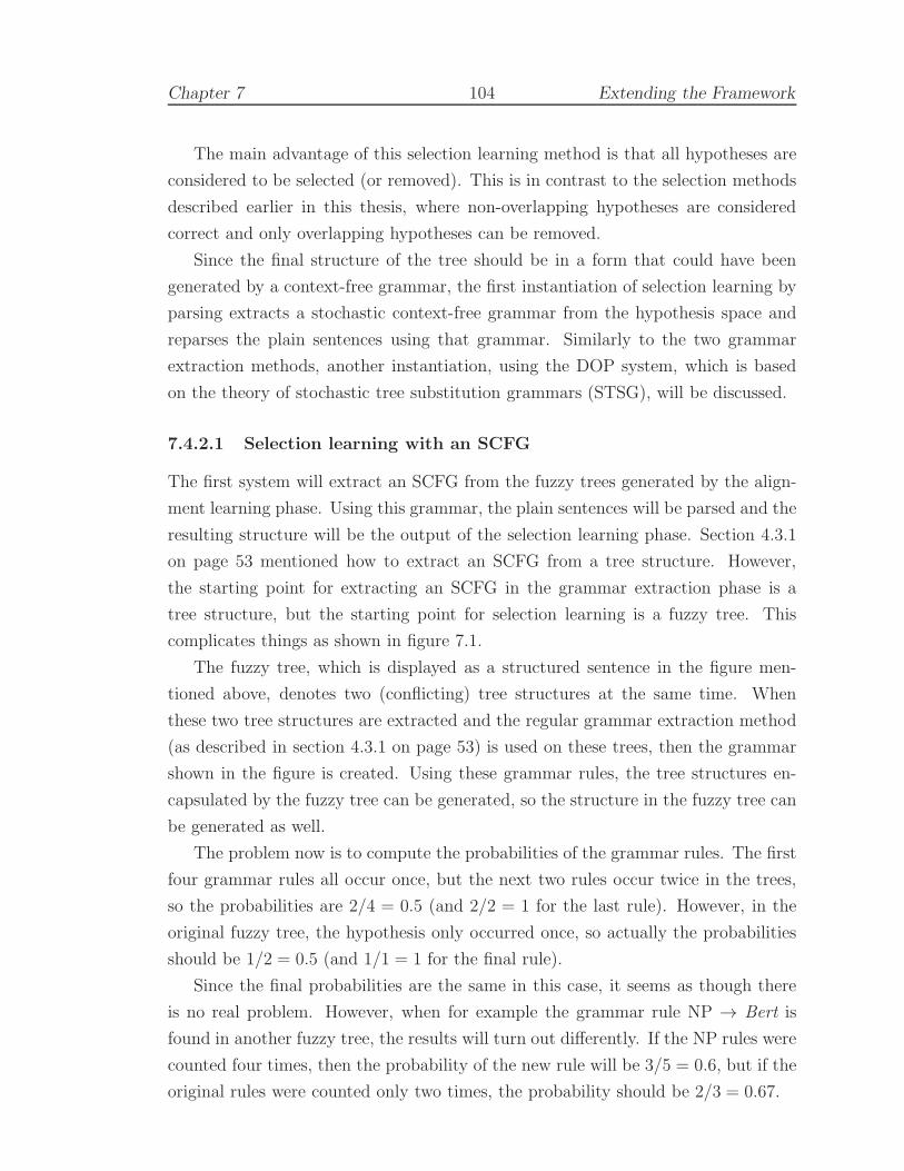
Chapter 7 104 Extending the Framework
The main advantage of this selection learning method is that all hypotheses are
considered to be selected (or removed). This is in contrast to the selection methods
described earlier in this thesis, where non-overlapping hypotheses are considered
correct and only overlapping hypotheses can be removed.
Since the final structure of the tree should be in a form that could have been
generated by a context-free grammar, the first instantiation of selection learning by
parsing extracts a stochastic context-free grammar from the hypothesis space and
reparses the plain sentences using that grammar. Similarly to the two grammar
extraction methods, another instantiation, using the DOP system, which is based
on the theory of stochastic tree substitution grammars (STSG), will be discussed.
7.4.2.1 Selection learning with an SCFG
The first system will extract an SCFG from the fuzzy trees generated by the align-
ment learning phase. Using this grammar, the plain sentences will be parsed and the
resulting structure will be the output of the selection learning phase. Section 4.3.1
on page 53 mentioned how to extract an SCFG from a tree structure. However,
the starting point for extracting an SCFG in the grammar extraction phase is a
tree structure, but the starting point for selection learning is a fuzzy tree. This
complicates things as shown in figure 7.1.
The fuzzy tree, which is displayed as a structured sentence in the figure men-
tioned above, denotes two (conflicting) tree structures at the same time. When
these two tree structures are extracted and the regular grammar extraction method
(as described in section 4.3.1 on page 53) is used on these trees, then the grammar
shown in the figure is created. Using these grammar rules, the tree structures en-
capsulated by the fuzzy tree can be generated, so the structure in the fuzzy tree can
be generated as well.
The problem now is to compute the probabilities of the grammar rules. The first
four grammar rules all occur once, but the next two rules occur twice in the trees,
so the probabilities are 2/4 = 0.5 (and 2/2 = 1 for the last rule). However, in the
original fuzzy tree, the hypothesis only occurred once, so actually the probabilities
should be 1/2 = 0.5 (and 1/1 = 1 for the final rule).
Since the final probabilities are the same in this case, it seems as though there
is no real problem. However, when for example the grammar rule NP → Bert is
found in another fuzzy tree, the results will turn out differently. If the NP rules were
counted four times, then the probability of the new rule will be 3/5 = 0.6, but if the
original rules were counted only two times, the probability should be 2/3 = 0.67.

Chapter 7 105 Extending the Framework
Figure 7.1 Extracting an SCFG from a fuzzy tree
[S[X1[NPBert]NP [X2
[Vsees]V]X1[NPErnie]NP]X2
]S
S
X1
NP
Bert
V
sees
NP
Ernie
S
NP
Bert
X2
V
sees
NP
Ernie
S → X1 NP 1/2=0.5S → NP X2 1/2=0.5X1 → NP V 1/1=1X2 → V NP 1/1=1NP → Bert 1/2=0.5 or 2/4=0.5NP → Ernie 1/2=0.5 or 2/4=0.5V → sees 1/1=1 or 2/2=1
7.4.2.2 Selection learning with an STSG
Similarly to the approach taken in section 4.3, it is possible to extract a stochastic
tree substitution grammar instead of a stochastic context free grammar to use for
selection learning. The advantage of this type of grammar is that it can capture a
wider variety of stochastic dependencies between words in subtrees.
Extracting an SCFG from a fuzzy trees is not entirely without problems, as
shown in the previous section and extracting an STSG has the same problem, only
worse. The main problem with extracting an SCFG is that grammar rules that
are contained in overlapping constituents can be counted in different ways. When
extracting subtrees, this occurs much more frequently. On the other hand, once this
problem has been solved for the SCFG case, it is also solved for the STSG case.
7.5 ABL with Data-Oriented Translation
Recently there has been research into a data-oriented approach to machine transla-
tion (Poutsma, 2000a,b; Way, 1999). The idea of the systems (based on DOP) is to
translate sentences by parsing the source sentence using elementary trees extracted
from a bilingually annotated, paired treebank. Each of the elementary subtrees in

Chapter 7 106 Extending the Framework
the source language is linked to a subtree in the target language, so when a parse
of the source language is found, the parse and thus the translated sentence in the
target language follows automatically.
One of the main problems with DOP is that an initial set of elementary subtrees
is needed. With these machine translation techniques, the problem is even worse,
since linked3 (bi-lingual) subtrees are needed. Building such treebanks by hand is
highly impractical. However, in section 4.3.2 on page 54, it was shown that ABL can
learn a stochastic tree substitution grammar. This type of grammar is the basis of
the DOP framework. By adapting ABL slightly, it can also be used to learn linked
STSGs.
Instead of applying ABL to a set of sentences, ABL is given a set of pairs of
sentences, where one sentence of the pair translates to the other sentence. If for
example the sentences in figure 7.2 are given to ABL (the English sentences on
the left-hand side translate to the Dutch sentences on the right-hand side), the
hypotheses with types E2 and D2 are introduced.
Figure 7.2 Learning structure in sentence pairs
English Dutch[Bert sees [Ernie]E2
]E1[Bert ziet [Ernie]D2
]D1
[Bert sees [Big Bird]E2]E1
[Bert ziet [Pino]D2]D1
When a hypothesis is introduced in the source and target sentences, a hypothet-
ical link is also introduced between the two. A link indicates that the two phrases
below the linked nodes are translation equivalent. Figure 7.3 shows how the sen-
tences of figure 7.2 are linked. The link between E1 and D1 indicates that the two
sentences are translation equivalent and the same applies to the phrases below the
E2 and D2 non-terminals.
When more than one pair of hypotheses is found in the sentences, all possible
combinations of hypothetical links are introduced. This is needed since different
languages may have a different word order. For example the sentences as given
in 43 (taken from (Poutsma, 2000b)) show that the subject of the first sentence
occurs as the object of the second sentence. If these sentences are aligned against
sentences where the subjects and objects are different, it is unclear whether the
hypothesis containing John should be linked against the hypothesis Jean or Marie,
since both sentences will receive two hypotheses.
3Subtrees are linked when they are translation equivalent.

Chapter 7 107 Extending the Framework
Figure 7.3 Linked tree structures
E1
Bert sees E2
Ernie
D1
Bert ziet D2
Ernie
E1
Bert sees E2
Big Bird
D1
Bert ziet D2
Pino
(43) a. John likes Mary
b. Marie plaıt a Jean
After the alignment learning phase, the hypotheses need to be disambiguated
as usual, but since the system also introduces ambiguous links, these need to be
disambiguated as well. The best links can be chosen by computing the probability
that a hypothesis in one language is linked against the hypothesis in the other
language. In the end, links that occur more often will be correct. For example,
John will be more often linked with Jean than with Marie, when other sentences
containing John and Jean but not Marie occur in the corpus.
7.6 (Semi-)Supervised Alignment-Based Learning
Unsupervised grammar induction systems like ABL do not have any knowledge
about what the final treebank should look like, since unsupervised systems are not
guided towards the wanted structure. Although, they usually yield less than perfect

Chapter 7 108 Extending the Framework
results, these systems are still useful, for example when building a treebank of an
unknown language, when no experts are available or when results are needed quickly.
On the other hand, when experts are available, when more precise results are
needed or when there are no pressing time restrictions, the resulting treebank gen-
erated by an unsupervised grammar induction system might not be satisfactory.
One possible way to use an unsupervised induction system for the generation of
high quality treebanks is to improve the quality of the generated treebank by post-
processing done by experts. As an example, the Penn Treebank, which is probably
the most widely used treebank to date, was annotated in two phases (automatic
structure induction followed by manual post-processing) (Marcus et al., 1993).
A more interesting approach to building a structured corpus, instead of choosing
for one of the two possibilities of building a treebank (using an induction system or
annotating the treebank by hand), would be to combine the best of both methods.
This should result in a system that suggests possible tree structures for the expert
to choose from and it should learn from the choices made by the expert in parallel.
The ABL system can be adapted into a system, called (Semi-) Supervised ABL
(SABL), that indicates reasonably good tree structures and learns from the expert’s
choices. The only changes needed in the algorithm occur in the selection learning
phase:
Select n-best hypotheses Instead of selecting the best hypotheses only, as in
standard ABL, let the system select the n (say 5) best hypotheses. These
hypotheses are presented to the expert, who chooses the correct one or, if the
correct one is not present in the set of n-best hypotheses, adds it manually.
Learn from the expert’s choice ABL’s selection of the best hypotheses from the
hypothesis universe is guided by a probabilistic evaluation function. In order
to learn from the choices made by the expert, the probabilities of the chosen
hypotheses should be changed:
• If the correct hypothesis (i.e. the hypothesis chosen by the expert) was
already present in the hypothesis universe, the probability of that hy-
pothesis should be increased. When a hypothesis has a high probability,
it will have a higher chance to be selected next time.
• If the correct hypothesis was not present in the hypothesis universe, it
should be inserted and the probabilities of the hypotheses should be ad-
justed. Since it was the preferred hypothesis, its probability should be

Chapter 7 109 Extending the Framework
increased as if the hypothesis was present in the hypothesis universe al-
ready.
Varying the amount of increase in probability, changes the learning properties of
the system. A small amount of increase makes the system a slow learner, while a
large amount of increase may over-fit the system.
Using an unsupervised grammar induction system and manual annotation are
two opposing methods in building a treebank. SABL can be placed anywhere be-
tween the two extremes. By varying how many of the proposed hypotheses are
actually used, SABL can be adjusted to work anywhere in the continuum between
hand annotation and fully automatic structuring of sentences.
7.7 More corpora
Along with extending the ABL system, more extensive testing of the current system
is needed as well. Testing ABL on different corpora will yield a deeper insight into
the properties and (possible) shortcomings of ABL. Future research can take several
different directions when evaluating ABL. Interesting future work will investigate
• the linguistic properties of ABL,
• the performance of ABL in a larger domain,
• the application of ABL on completely different data sets.
Chapter 5 on page 57 showed that ABL performs reasonably well on corpora of
mainly right branching languages. It clearly outperformed the system that generates
a randomly chosen left or right branching structure.
It was claimed that ABL will perform equally well on corpora of left or right
branching languages. This claim needs to be tested on corpora of for example
Japanese. Since the ABL system does not have a built-in preference for left or right
branching structures, it can be expected that ABL will perform equally well on a
corpus of a left or right branching language.
A right branching system outperforms ABL on an English or Dutch corpus and a
left branching system will probably outperform ABL on a Japanese corpus. However,
this is an unfair comparison, since the left and right branching systems are biased
towards the language in the corpus (whereas ABL is not). The independent random
system as described in chapter 5 can, like ABL, be expected to perform similarly on

Chapter 7 110 Extending the Framework
a Japanese corpus. Therefore, ABL will probably outperform the random system
on a corpus of a left branching language, too.
ABL has been tested on two corpora which both are taken from a limited domain
(that of flight information and public transportation). Next to these two corpora,
the ABL system has been applied to the large domain WSJ corpus. This showed
that it is practically possible to use this system on such a corpus.
First tests on a larger domain corpus show the need for loosening the exact
match of words, as discussed in section 7.2. Since the size of the vocabulary in
a large domain is larger, it will help the system match non-function words. This
indicates that more research can be done in this direction.
Finally, the system can also be applied to different types of corpora. Although
the original system is developed to find syntactic structure in natural language
sentences, it might be interesting to see how well ABL can find structure in other
types of data, which can be (but are not limited to) for example:
Morphology There has been some work in the unsupervised learning of morpho-
logical structure, e.g. Clark (2001a); Gaussier (1999); Goldsmith (2001). It is
also possible to apply ABL to a set of words, instead of a set of plain sentences,
to find inner-word structure. ABL will then align characters (phonemes, or
plain letters) while the rest of the system remains the same.
As an example, consider aligning the words /r2nIN/ (running) and /wO:kIN/
(walking) as shown in 44 (taken from (Longman, 1995)). From this alignment,
the syllables /r2n/ (run), /wO:k/ (walk), and /IN/ (-ing) can be found. Simi-
larly, applying the algorithm to compound words will decompose these. When
applying ABL to a collection of words, a hierarchically deeper structure can
be found.
(44) a. r2nIN
running
b. wO:kIN
walking
Music A central topic in musicology is to construct formal descriptions of musical
structures. Where in linguistics it is uncontroversial to use tree structures to
describe the syntactic structure of sentences, in musicology similar structures4
are used (Sloboda, 1985).
4Recently, structured musical data has become available (Schaffrath, 1995).

Chapter 7 111 Extending the Framework
Musical pieces can be structured according to different viewpoints. Lerdahl
and Jackendoff (1983) recognise the following components on which a musical
piece can be structured:
Grouping structure This component indicates how a musical piece can be
subdivided into sections, phrases and motives.
Metrical structure A musical piece contains strong and weak beats, which
are often repeated in a regular way within a number of hierarchical levels.
This component structures a musical piece based on the metric structure
within that piece.
Time-span reduction Amusical piece can be structured based on the pitches.
Each of the pitches can be placed in a hierarchy of structural importance
based on their position in metrical and grouping structure.
Prolongational reduction The pitches in a musical piece can also be struc-
tured in a hierarchy that “expresses harmonic and melodic tension and
relaxation, continuity and progression.”
Next to these viewpoints, there are other dimensions of musical structure, such
as timbre, dynamics, and motivic-thematic processes. However, these are not
hierarchical in nature.
A good system that learns structure in music will need to be able to recog-
nise (the combinations of) these different viewpoints with their corresponding
parameters. If ABL is to be used in this field, several adaptions are needed.
Furthermore, musical pieces are much longer than natural language sentences.
Since the ABL system relies on the edit distance algorithm, it has difficulties
with longer input.
DNA structure DNA (or RNA) is usually described by naming the bases in a
DNA strand. Bases are the building blocks of DNA and each base is denoted
by a letter. Each base is one of A, G, C, or T. A piece of DNA is thus described
by a list containing these four letters. In the end, the parts of a DNA string
of bases denoted by letters can be combined to form larger molecules.
From the DNA molecules, RNA is extracted. RNA is a molecule that is
composed of (copies of) parts of the original DNA molecule. The combinations
of adjacent bases in the RNA can be seen as blueprints for amino acids. These
amino acids can then form proteins. The main problem here is to find which

Chapter 7 112 Extending the Framework
parts of the DNA molecules contain useful information and will be copied
into an RNA strand (Durbin, 2001; Gusfield, 1997; Sankoff and Kruskal, 1999;
Searls, 1994).
Figure 7.4 illustrates how RNA bases combine into amino acids, which again
combine into a protein. This hierarchy might be found when applying ABL
to the bases of RNA.
Figure 7.4 Structure in RNA
Protein
Amino
Base Base Base
Amino
Base Base Base
Amino
Base Base Base
Amino
Base Base Base
The main problem with these types of data (e.g. musical and DNA/RNA) is
that there are no clear “sentences”. Whereas musical data might be chunked into
phrases, this is clearly more difficult with DNA or RNA information. The current
implementation of ABL is inherently slow when applied to very large strings (of for
example over 10,000 symbols), since the time of the edit distance algorithm is in the
order of the squared length of the string.

Chapter 8
ConclusionDe antwoorden zijn altijd al aanwezig.
— Steve Vai (Passion and Warfare)
Alignment-Based Learning (ABL) is an unsupervised grammar induction system
that generates a labelled, bracketed version of the unstructured input corpus. The
goal of the system is to learn syntactic structure in plain sentences using a minimum
of information. This implies that no a priori knowledge of the language of the input
corpus (or of any other particular language in general) is assumed, not even part-of-
speech tags of the words. This shows how an empiricist system can learn syntactic
structure in practice.
The system is a combination of several known techniques, which are used in
completely new ways. It relies heavily on Harris’s notion of substitutability and
Wagner and Fischer’s edit distance algorithm. Implementing a system based on
the notion of substitutability using the edit distance algorithm yields several new
insights into these established methods.
Harris (1951) states that substitutable segments are descriptively equivalent.
This means that everything that can be said about one segment can also be said
about the other segment. He also describes a method to find the substitutable
segments by comparing sentences: substitutable segments are parts of utterances
that can be substituted for each other in different contexts. This idea is used as a
starting point for the alignment learning phase.
Harris never mentioned the practical problems with this approach. The first
problem to tackle is how to find the substitutable parts of two sentences. In ABL,
113

Chapter 8 114 Conclusion
the edit distance algorithm is used for this task. This is reflected in the alignment
learning phase of the system.
The second problem of Harris’s notion of substitutability is that when search-
ing for substitutable segments, at some point conflicting (overlapping) substitutable
segments are found. The selection learning phase of ABL tries to disambiguate be-
tween the possible (context-free) syntactic structures found by the alignment learn-
ing phase.
ABL consists thus of two phases, alignment learning and selection learning. The
first phase generates a search space of possible constituents and the second phase
searches this space to select the best constituents. The selected constituents are
stored in the structured output corpus.
During the alignment learning phase, pairs of sentences are aligned against each
other. This can be done in several different ways. In this thesis three systems are de-
scribed. The first uses the instantiation of the edit distance algorithm (Wagner and
Fischer, 1974) which finds the longest common subsequence between two sentences.
The second is an adjusted version of the longest common subsequence algorithm
which prefers not to link equal words in the two sentences that are relatively far
apart (i.e. one word in the beginning of the sentence and the other word at the
end of the other sentence). The third system, which does not use the edit distance
algorithm, finds all possible alignments if there are more than one.
Aligning sentences against each other uncovers parts of the sentences that are
equal (or unequal) in both. The unequal parts of the sentences are stored as hy-
potheses, denoting possible constituents. This step is in line with Harris’s notion of
substitutability, where parts of sentences that occur in the same context are recog-
nised as constituents.
The alignment learning phase may at some point introduce hypotheses that over-
lap each other. Overlapping hypotheses are unwanted, since their structure could
never have been generated by a context-free (or mildly context-sensitive) grammar.
The selection learning phase selects hypotheses from the set of hypothesis generated
by the alignment learning phase, which resolves all overlapping hypotheses. This
can be done in several different ways.
First, a non-probabilistic method is described where hypotheses that are learned
earlier are considered correct. The main disadvantage of this system is that incor-
rectly learned hypotheses can never be corrected, when they are learned early. The
other systems that have been implemented both have a probabilistic basis. The
probability of each (overlapping) hypothesis is computed using counts from the hy-

Chapter 8 115 Conclusion
potheses in the set of all hypotheses generated by the alignment learning phase.
The probabilities of the separate hypotheses are combined and the combination of
(non-overlapping) hypotheses with the highest combined probability is selected.
The probabilistic selection learning methods allow for a gradient range of knowl-
edge about hypotheses, instead of an absolute yes/no distinction. This (potentially)
solves many of the problems that used to be attributed to Harris’s notion of substi-
tutability (e.g. the problems introduced by Chomsky (1955) and Pinker (1994) as
discussed in section 2.5.2).
The ABL system, consisting of the alignment and selection learning phase, can
be extended with a grammar extraction and parsing phase. This system is called
parseABL. The output of this system is a structured corpus (similar to the ABL
system) and a stochastic grammar (a context-free or tree substitution grammar).
Reparsing the plain sentences using an extracted grammar does not improve the
quality resulting structured corpus, however.
No language dependent assumptions are considered by the system, however, it
relies on some language independent assumptions. First of all, Harris’s idea of
substitutability gives a way of finding possible constituents. This results in a richly
structured version of the input sentences. For evaluation purposes, an underlying
context-free grammar constraint is imposed on this data structure. Note that this
is not a necessary assumption for the system. It is not a feature of the system.
When applying the system to real-life data sets, some striking features of the
system arise. The structured corpora generated by ABL by applying it to the ATIS,
OVIS and WSJ corpora all contain recursive structures. This is interesting since
ABL is able to find recursive constituents by considering only a finite number of
sentences.
The ABL system has been applied to three corpora, the ATIS, OVIS and WSJ
corpus. On all corpora, ABL yielded encouraging results. To our knowledge, this is
the first time an unsupervised learning system has been applied to the plain WSJ
corpus. Additionally, ABL has been compared to the EMILE system (Adriaans,
1992), which it clearly outperforms. More recently, Clark (2001b) has compared
his system against ABL. These results are not completely comparable, since his
system is bootstrapped using much more information. Even then, ABL’s results are
competitive.
BibliographyWeiner’s Law of Libraries:
There are no answers, only cross references.
— Anonymous
ACL (1995). Proceedings of the 33th Annual Meeting of the Association for Com-
putational Linguistics (ACL). Association for Computational Linguistics (ACL).
ACL (1997). Proceedings of the 35th Annual Meeting of the Association for Com-
putational Linguistics (ACL) and the 8th Meeting of the European Chapter of the
Association for Computational Linguistics (EACL); Madrid, Spain. Association
for Computational Linguistics (ACL).
Adriaans, P., Trautwein, M., and Vervoort, M. (2000). Towards high speed grammar
induction on large text corpora. In Hlavac, V. Feffrey, G. and Wiedermann,
J., editors, SOFSEM 2000: Theory and Practice of Informatics, volume 1963
of Lecture Notes in Computer Science, pages 173–186. Springer-Verlag, Berlin
Heidelberg, Germany.
Adriaans, P. W. (1992). Language Learning from a Categorial Perspective. PhD
thesis, University of Amsterdam, Amsterdam, the Netherlands.
Adriaans, P. W. (1999). Learning shallow context-free languages under simple dis-
tributions. Technical Report PP-1999-13, Institute for Logic, Language and Com-
putation (ILLC), Amsterdam, the Netherlands.
Allen, J. (1995). Natural Language Understanding. Benjamin/Cummings, Redwood
City:CA, USA, 2nd edition.
116
117 Bibliography
Baker, J. (1979). Trainable grammars for speech recognition. In Wolf, J. and Klatt,
D., editors, Speech Communication Papers for the Ninety-seventh Meeting of the
Acoustical Society of America, pages 547–550.
Bellman, R. E. (1957). Dynamic Programming. Princeton University Press, Prince-
ton:NJ, USA.
Black, E., Abney, S., Flickinger, D., Gdaniec, C., Grishman, R., Harrison, P., Hin-
dle, D., Ingria, R., Jelinek, F., Klavans, J., Liberman, M., Marcus, M., Roukos, S.,
Santorini, B., and Strzalkowski, T. (1991). A procedure for quantitatively compar-
ing the syntactic coverage of English grammars. In Proceedings of a Workshop—
Speech and Natural Language, pages 306–311.
Bloomfield, L. (1933). Language. George Allen & Unwin Limited, London, UK,
reprinted 1970 edition.
Bod, R. (1995). Enriching Linguistics with Statistics: Performance Models of Natu-
ral Language. PhD thesis, University of Amsterdam, Amsterdam, the Netherlands.
Bod, R. (1998). Beyond Grammar—An Experience-Based Theory of Language, vol-
ume 88 of CSLI Lecture Notes. Center for Study of Language and Information
(CSLI) Publications, Stanford:CA, USA.
Bod, R. (2000). Parsing with the shortest derivation. In COLING (2000), pages
69–75.
Bonnema, R., Bod, R., and Scha, R. (1997). A DOP model for semantic interpre-
tation. In ACL (1997), pages 159–167.
Booth, T. (1969). Probabilistic representation of formal languages. In Conference
Record of 1969 Tenth Annual Symposium on Switching and Automata Theory,
pages 74–81.
Brent, M. R. (1999). An efficient, probabilistically sound algorithm for segmentation
and word discovery. Machine Learning, 34:71–105.
Brill, E. (1993). Automatic grammar induction and parsing free text: A
transformation-based approach. In Proceedings of the 31th Annual Meeting of
the Association for Computational Linguistics (ACL); Columbus:OH, USA, pages
259–265. Association for Computational Linguistics (ACL).

118 Bibliography
Caraballo, S. A. and Charniak, E. (1998). New figures of merit for best-first proba-
bilistic chart parsing. Computational Linguistics, 24(2):275–298.
Carroll, L. (1982). Alice’s adventures in wonderland. In The Complete Illustrated
Works of Lewis Carroll, pages 17–114. Chancellor Press, London, UK, 1st (1993)
edition. First published in 1865.
Charniak, E. (1993). Statistical Language Learning. Massachusetts Institute of
Technology Press, Cambridge:MA, USA and London, UK.
Charniak, E. (1997). Statistical parsing with a context-free grammar and word
statistics. In Proceedings of the Fourteenth National Conference on Artificial In-
telligence, pages 598–603. American Association for Artificial Intelligence (AAAI).
Chen, S. F. (1995). Bayesian grammar induction for language modeling. In ACL
(1995), pages 228–235.
Chen, S. F. and Goodman, J. (1996). An empirical study of smoothing techniques
for language modeling. In Proceedings of the 34th Annual Meeting of the Asso-
ciation for Computational Linguistics (ACL); Santa Cruz:CA, USA. Association
for Computational Linguistics (ACL).
Chen, S. F. and Goodman, J. (1998). An empirical study of smoothing techniques
for language modeling. Technical Report TR-10-98, Harvard University, Cam-
bridge:MA, USA.
Chomsky, N. (1955). The Logical Structure of Linguistic Theory. Plenum Press,
New York:NY, USA, reprinted 1975 edition.
Chomsky, N. (1965). Aspects of the Theory of Syntax. Massachusetts Institute of
Technology Press, Cambridge:MA, USA and London, UK. 3rd paperback printing.
Chomsky, N. (1986). Knowledge of Language — Its Nature, Origin, and Use. Praeger
Publishers, New York:NY, USA.
Clark, A. (2001a). Learning morphology with pair hidden markov models. In Pro-
ceedings of the Student Research Workshop of the 39th Annual Meeting of the As-
sociation for Computational Linguistics (ACL) and the 10th Meeting of the Euro-
pean Chapter of the Association for Computational Linguistics (EACL); Toulouse,
France, pages 55–60. Association for Computational Linguistics (ACL).

119 Bibliography
Clark, A. (2001b). Unsupervised induction of stochastic context-free grammars using
distributional clustering. In CoNLL (2001), pages 105–112.
COLING (2000). Proceedings of the 18th International Conference on Computational
Linguistics (COLING); Saarbrucken, Germany. Association for Computational
Linguistics (ACL).
Collins, M. (1997). Three generative, lexicalised models for statistical parsing. In
ACL (1997), pages 16–23.
CoNLL (2001). Proceedings of the Workshop on Computational Natural Language
Learning held at the 39th Annual Meeting of the Association for Computational
Linguistics (ACL) and the 10th Meeting of the European Chapter of the Associ-
ation for Computational Linguistics (EACL); Toulouse, France. Association for
Computational Linguistics (ACL).
Cook, C. M., Rosenfeld, A., and Aronson, A. R. (1976). Grammatical inference by
hill climbing. Informational Sciences, 10:59–80.
Cook, D. J. and Holder, L. B. (1994). Substructure discovery using minimum de-
scription length and background knowledge. Journal of Artificial Intelligence
Research, 1:231–255.
de Marcken, C. (1995). Acquiring a lexicon from unsegmented speech. In Pro-
ceedings of the Student Session of the 33th Annual Meeting of the Association
for Computational Linguistics (ACL). Association for Computational Linguistics
(ACL).
de Marcken, C. (1999). The unsupervised acquisition of a lexicon from continu-
ous speech. Technical Report AI Memo 1558, CBCL Memo 129, Massachusetts
Institute of Technology, Artificial Intelligence Laboratory, Center for Biological
and Computational Learning Department of Brain and Cognitive Sciences, Cam-
bridge:MA, USA.
de Marcken, C. G. (1996). Unsupervised Language Acquisition. PhD thesis, Mas-
sachusetts Institute of Technology, Cambridge:MA, USA.
Dejean, H. (2000). ALLiS: a symbolic learning system for natural language learn-
ing. In Cardie, C., Daelemans, W., Nedellec, C., and Tjong Kim Sang, E., editors,

120 Bibliography
Proceedings of the Fourth Conference on Computational Natural Language Learn-
ing and of the Second Learning Language in Logic Workshop; Lisbon, Portugal,
pages 95–98. Held in cooperation with ICGI-2000.
Dornenburg, E. (1997). Extensions of the EMILE algorithm for inductive learning
of context-free grammars. Master’s thesis, University of Dortmund, Dortmund,
Germany.
Duda, R. O. and Hart, P. E. (1973). Pattern Classification and Scene Analysis.
John Wiley and Sons, New York:NY, USA.
Durbin, R. (2001). Interpreting the human genome sequence, using stochastic gram-
mars. In Proceedings of the 39th Annual Meeting of the Association for Compu-
tational Linguistics (ACL) and the 10th Meeting of the European Chapter of the
Association for Computational Linguistics (EACL); Toulouse, France. Associa-
tion for Computational Linguistics (ACL). Invited talk.
Finch, S. and Chater, N. (1992). Bootstrapping syntactic categories using statistical
methods. In Daelemans, W. and Powers, D., editors, Background and Experiments
in Machine Learning of Natural Language: Proceedings First SHOE Workshop,
pages 230–235, Tilburg, the Netherlands. Institute for Language Technology and
AI Tilburg University.
Frayn, M. (1965). The Tin Men. Collins Fontana Books.
Frege, G. (1879). Begriffsschrift, eine der Arithmetischen Nachgebildete Formel-
sprache des Reines Denkens. Verlag von Louis Nebert, Halle, Germany.
Gaussier, E. (1999). Unsupervised learning of derivational morphology from inflec-
tional lexicons. In Kehler and Stolcke (1999b).
Gold, E. (1967). Language identification in the limit. Information and Control,
10:447–474.
Goldsmith, J. (2001). Unsupervised learning of the morphology of a natural lan-
guage. Computational Linguistics, 27(2):153–198.
Goossens, M., Mittelbach, F., and Samarin, A. (1994). The LATEX Companion.
Addison-Wesley Publishing Company, Reading:MA, USA.
Goossens, M., Rahtz, S., and Mittelbach, F. (1997). The LATEX Graphics Companion.
Addison-Wesley Publishing Company, Reading:MA, USA.

121 Bibliography
Grune, D. and Jacobs, C. (1990). Parsing Techniques—A Practical Guide. Ellis
Horwood Limited, Chichester, UK. Printout by the authors.
Grunwald, P. (1994). A minimum description length approach to grammar inference.
In Scheler, G., Wernter, S., and Riloff, E., editors, Connectionist, Statistical and
Symbolic Approaches to Learning for Natural Language, volume 1004 of Lecture
Notes in AI, pages 203–216. Springer-Verlag, Berlin Heidelberg, Germany.
Gusfield, D. (1997). Algorithms on strings, trees, and sequences: computer sci-
ence and computational biology. Cambridge University Press, Cambridge, UK.
Reprinted 1999 (with corrections).
Harris, Z. S. (1951). Structural Linguistics. University of Chicago Press, Chicago:IL,
USA and London, UK, 7th (1966) edition. Formerly Entitled: Methods in Struc-
tural Linguistics.
Honkela, T., Pulkki, V., and Kohonen, T. (1995). Contextual relations of words
in grimm tales, analyzed by self-organizing map. In Fogerlman-Soulie, F. and
Gallinari, P., editors, Proceedings of the International Conference on Artificial
Neural Networks; Paris, France, pages 3–7.
Horning, J. J. (1969). A study of grammatical inference. PhD thesis, Stanford
University, Stanford:CA, USA.
Hubbard, T. J. P., Lesk, A. M., and Tramontano, A. (1996). Gathering them into
the fold. Nature Structural Biology, 3(4):313.
Huckle, C. C. (1995). Grouping words using statistical context. In ACL (1995).
Hwa, R. (1999). Supervised grammar induction using training data with limited
constituent information. In Proceedings of the 37th Annual Meeting of the Asso-
ciation for Computational Linguistics (ACL); Maryland:MD, USA, pages 73–79.
Association for Computational Linguistics (ACL).
Johnson, S. C. (1979). Yacc: Yet another compiler-compiler. In UNIX Programmer’s
Manual, pages 353–387. Holt, Rinehart, and Winston, New York:NY, USA. Vol.
2.
Jurafsky, D. and Martin, J. H. (2000). Speech and Language Processing. Prentice
Hall, Englewood Cliffs:NJ, USA.

122 Bibliography
Kay, J. and Kummerfeld, B. (1989). C Programming in a UNIX Environment. Inter-
national Computer Science Series. Addison-Wesley Publishing Company, Read-
ing:MA, USA.
Kehler, A. and Stolcke, A. (1999a). Preface. In Kehler and Stolcke (1999b).
Kehler, A. and Stolcke, A., editors (1999b). Proceedings of a Workshop—
Unsupervised Learning in Natural Language Processing; Maryland:MD, USA.
Kernighan, B. W. and Ritchie, D. M. (1988). The C Programming Language. Pren-
tice Hall Software Series. Prentice Hall, Englewood Cliffs:NJ, USA, 2nd edition.
ANSI C.
Klein, D. and Manning, C. D. (2001). Distributional phrase structure indiction. In
CoNLL (2001), pages 113–120.
Knight, K. and Yamada, K. (1999). A computational approach to deciphering
unknown scripts. In Kehler and Stolcke (1999b), pages 37–44.
Knuth, D. E. (1986). The TEXbook. Addison-Wesley Publishing Company, Read-
ing:MA, USA. Reprinted with corrections 1993.
Knuth, D. E. (1996). Are toy problems useful? In Selected Papers in Computer
Science. Center for Study of Language and Information (CSLI) Publications, Stan-
ford:CA, USA.
Lamport, L. (1994). LATEX: A Document Preparation System. Addison-Wesley
Publishing Company, Reading:MA, USA, 2nd edition.
Lari, K. and Young, S. (1990). The estimation of stochastic context-free grammars
using the inside-outside algorithm. Computer Speech and Language, 4(35–56).
Lee, L. (1996). Learning of context-free languages: A survey of the literature.
Technical Report TR-12-96, Harvard University, Cambridge:MA, USA.
Lerdahl, F. and Jackendoff, R. S. (1983). A generative theory of tonal music. Mas-
sachusetts Institute of Technology Press, Cambridge:MA, USA and London, UK.
Levenshtein, V. I. (1965). Binary codes capable of correcting deletions, insertions,
and reversals. Doklady Akademii Nauk SSR, 163(4):845–848. Original in Russian.
Li, M. and Vitanyi, P. M. B. (1991). Learning simple concepts under simple distri-
butions. SIAM Journal of Computing, 20(5):911–935.

123 Bibliography
Lippman, S. B. (1991). C++ Primer. Addison-Wesley Publishing Company, Read-
ing:MA, USA, 2nd edition. Reprinted with corrections February 1993.
Longman (1995). Longman Dictionary of Contemporary English. Longman Group
Ltd, Essex, UK, 3rd edition.
Losee, R. M. (1996). Learning syntactic rules and tags with genetic algorithm
for information retrieval and filtering: An empirical basis for grammatical rules.
Information Processing & Management, 32(2):185–197.
Magerman, D. M. and Marcus, M. P. (1990). Parsing a natural language using mu-
tual information statistics. In Proceedings of the Eighth National Conference on
Artificial Intelligence, pages 984–989. American Association for Artificial Intelli-
gence (AAAI).
Marcus, M., Santorini, B., and Marcinkiewicz, M. (1993). Building a large annotated
corpus of English: the Penn treebank. Computational Linguistics, 19(2):313–330.
Montague, R. (1974). The proper treatment of quantification in ordinary English.
In Thomason, R. H., editor, Formal Philosophy — Selected Papers of Richard
Montague, chapter 8, pages 247–270. Yale University Press, New Haven:CT, USA
and London, UK.
Nakamura, K. and Ishiwata, T. (2000). Synthesizing context free grammars from
sample strings based on inductive CYK algorithm. In Oliveira (2000), pages 186–
195.
Nevado, F., Sanchez, J.-A., and Benedı, J.-M. (2000). Combination of estimation
algorithms and grammatical inference techniques to learn stochastic context-free
grammars. In Oliveira (2000), pages 196–206.
Nevill-Manning, C. G. and Witten, I. H. (1997). Identifying hierarchical structure
in sequences: A linear-time algorithm. Journal of Artificial Intelligence Research,
7:67–82.
Oliveira, A. L., editor (2000). Grammatical Inference: Algorithms and Applications
(ICGI); Lisbon, Portugal.
Osborne, M. (1994). Learning Unification-Based Natural Language Grammars. PhD
thesis, University of York, York, UK.

124 Bibliography
Pereira, F. and Schabes, Y. (1992). Inside-outside reestimation from partially brack-
eted corpora. In Proceedings of the 30th Annual Meeting of the Association for
Computational Linguistics (ACL); Newark:NJ, USA, pages 128–135. Association
for Computational Linguistics (ACL).
Pinker, S. (1984). Language learnability and language development. Harvard Uni-
versity Press, Cambridge:MA.
Pinker, S. (1994). The Language Instinct—The New Science of Language and Mind.
Penguin Books, Harmondsworth, Middlesex, UK.
Poutsma, A. (2000a). Data-Oriented Translation. In COLING (2000), pages 635–
641.
Poutsma, A. (2000b). Data-Oriented Translation—using the Data-Oriented Parsing
framework for machine translation. Master’s thesis, University of Amsterdam,
Amsterdam, the Netherlands.
Powers, D. M., editor (1997). Tutorial Notes—Machine Learning of Natural Lan-
guage; Madrid, Spain. Association for Computational Linguistics (ACL).
Redington, M., Chater, N., and Finch, S. (1998). Distributional information: A
powerful cue for acquiring syntactic categories. Cognitive Science, 22(4):425–469.
Russell, S. and Norvig, P. (1995). Artificial intelligence: a modern approach. Prentice
Hall, Englewood Cliffs:NJ, USA.
Sadler, V. and Vendelmans, R. (1990). Pilot implementation of a bilingual knowl-
edge bank. In Proceedings of the 13th International Conference on Computational
Linguistics (COLING); Helsinki, Finland, pages 449–451. Association for Com-
putational Linguistics (ACL).
Sakakibara, Y. (1992). Efficient learning of context-free grammars from positive
structural examples. Information and Computation, 97:23–60.
Sakakibara, Y. and Muramatsu, H. (2000). Learning context-free grammars from
partially structured examples. In Oliveira (2000), pages 229–240.
Sampson, G. (1995). English for the Computer — The SUSANNE Corpus and
Analytic Scheme. Clarendon Press (Oxford University Press), New York:NY,
USA.

125 Bibliography
Sampson, G. (1997). Educating Eve—The ‘Language Instinct’ Debate. Cassell,
London, UK and New York:NY, USA. Reprinted in paperback with minor changes
1999.
Sampson, G. (2000). A proposal for improving the measurement of parse accuracy.
International Journal of Corpus Linguistics, 5(1):53–68.
Sankoff, D. and Kruskal, J. (1999). Time Warps, String Edits, and
Macromolecules—The Theory and Practice of Sequence Comparison. The David
Hume Series (Philosophy and Cognitive Science Reissues). Center for Study of
Language and Information (CSLI) Publications, Stanford:CA, USA.
Schaffrath, H. (1995). The Essen folksong collection in the humdrum kern format.
D. Huron (ed.). Menlo Park:CA, USA. Center for Computer Assisted Research in
the Humanities.
Scholtes, J. C. and Bloembergen, S. (1992). Corpus based parsing with a self-
organizing neural net. In Proceedings of the International Joint Conference on
Neural Networks (IJCNN); Beijing, P.R. China.
Searls, D., editor (1994). The Computational Linguistics of Biological Sequences
(ACL’94 Tutorial Notes). Association for Computational Linguistics (ACL).
Sima’an, K. (1999). Learning Efficient Disambiguation. PhD thesis, Universteit
Utrecht, Utrecht, the Netherlands.
Simon, H. A. (1969). The Sciences of the Artificial. Massachusetts Institute of
Technology Press, Cambridge:MA, USA and London, UK, 1st edition.
Sloboda, J. A. (1985). The Musical Mind, volume 5 of Oxford Psychology Series.
Oxford University Press, New York:NY, USA.
Stolcke, A. (1994). Bayesian Learning of Probabilistic Language Models. PhD thesis,
University of California, Berkeley:CA, USA.
Stolcke, A. and Omohundro, S. (1994). Inducing probabilistic grammars by bayesian
model merging. In Proceedings of the Second International Conference on Gram-
mar Inference and Applications; Alicante, Spain, pages 106–118.
Stroustrup, B. (1997). The C++ Programming Language. Addison-Wesley Publish-
ing Company, Reading:MA, USA, 3rd edition.

126 Bibliography
Valiant, L. (1984). A theory of the learnable. Communications of the Association
for Computing Machinery, 27(11):1134–1142.
van Zaanen, M. (1997). Error correction using DOP. Master’s thesis, Vrije Univer-
siteit, Amsterdam, the Netherlands.
van Zaanen, M. (1999a). Bootstrapping structure using similarity. In Monachesi, P.,
editor, Computational Linguistics in the Netherlands 1999—Selected Papers from
the Tenth CLIN Meeting, pages 235–245, Utrecht, the Netherlands. Universteit
Utrecht.
van Zaanen, M. (1999b). Error correction using DOP. In De Roeck, A., editor, Pro-
ceedings of the Second UK Special Interest Group for Computational Linguistics
(CLUK2) (Second Issue), pages 1–12, Colchester, UK. University of Essex.
van Zaanen, M. (2000a). ABL: Alignment-Based Learning. In COLING (2000),
pages 961–967.
van Zaanen, M. (2000b). Bootstrapping syntax and recursion using Alignment-Based
Learning. In Langley, P., editor, Proceedings of the Seventeenth International
Conference on Machine Learning, pages 1063–1070, Stanford:CA, USA. Stanford
University.
van Zaanen, M. (2000c). Learning structure using Alignment Based Learning. In
Kilgarriff, A., Pearce, D., and Tiberius, C., editors, Proceedings of the Third An-
nual Doctoral Research Colloquium (CLUK), pages 75–82. Universities of Brighton
and Sussex.
van Zaanen, M. (2001). Building treebanks using a grammar induction system.
Technical Report TR2001.06, University of Leeds, Leeds, UK.
van Zaanen, M. (2002). Alignment-Based Learning versus Data-Oriented Parsing.
In Bod, R., Sima’an, K., and Scha, R., editors, Data Oriented Parsing. Center for
Study of Language and Information (CSLI) Publications, Stanford:CA, USA. to
be published.
van Zaanen, M. and Adriaans, P. (2001a). Alignment-Based Learning versus EMILE:
A comparison. In Proceedings of the Belgian-Dutch Conference on Artificial In-
telligence (BNAIC); Amsterdam, the Netherlands. to be published.

127 Bibliography
van Zaanen, M. and Adriaans, P. (2001b). Comparing two unsupervised gram-
mar induction systems: Alignment-Based Learning vs. EMILE. Technical Report
TR2001.05, University of Leeds, Leeds, UK.
Vervoort, M. R. (2000). Games, Walks and Grammars. PhD thesis, University of
Amsterdam, Amsterdam, the Netherlands.
Viterbi, A. (1967). Error bounds for convolutional codes and an asymptotically
optimum decoding algorithm. Institute of Electrical and Electronics Engineers
Transactions on Information Theory, 13:260–269.
Wagner, R. A. and Fischer, M. J. (1974). The string-to-string correction problem.
Journal of the Association for Computing Machinery, 21(1):168–173.
Way, A. (1999). A hybrid architecture for robust MT using LFG-DOP. Journal
of Experimental and Theoretical Artificial Intelligence, 11(4). Special Issue on
Memory-Based Language Processing.
Wolff, J. (1975). An algorithm for the segmentation of an artificial language ana-
logue. British Journal of Psychology, 66(1):79–90.
Wolff, J. (1977). The discovery of segments in natural language. British Journal of
Psychology, 68:97–106.
Wolff, J. (1996). Learning and reasoning as information compression by multiple
alignment, unification and search. In Gammerman, A., editor, Computational
Learning and Probabilistic Reasoning, chapter 4, pages 67–85. John Wiley & Sons,
Ltd., Chichester, UK.
Wolff, J. G. (1980). Language acquisition and the discovery of phrase structure.
Language and Speech, 23(3):255–269.
Wolff, J. G. (1982). Language acquisition, data compression and generalization.
Language and Communication, 2(1):57–89.
Wolff, J. G. (1988). Learning syntax and meanings through optimization and distri-
butional analysis. In Levy, Y., Schlesinger, I., and Braine, M., editors, Categories
and Processes in Language Acquisition, chapter 7, pages 179–215. Lawrence Erl-
baum, Hillsdale:NJ, USA.

128 Bibliography
Wolff, J. G. (1998a). Parsing as information compresion by multiple alignment,
unification and search: Examples. Technical report, University of Wales, Bangor,
UK.
Wolff, J. G. (1998b). Parsing as information compresion by multiple alignment,
unification and search: SP52. Technical report, University of Wales, Bangor, UK.
Younger, D. (1967). Recognition and parsing of context-free languages in time n3.
Information and Control, 10(2):189–208.