boston, usa, august 5-11, 2012 - international association for
TRANSCRIPT
Poster Session #2
Time: Thursday, August 9, 2012 PM
Paper Prepared for the 32nd General Conference of
The International Association for Research in Income and Wealth
Boston, USA, August 5-11, 2012
Wealth Distributions and Power Laws : Evidence from "Rich Lists”
Michal Brzezinski
For additional information please contact:
Name: Michal Brzezinski
Affiliation: University of Warsaw, Poland
Email Address: [email protected]
This paper is posted on the following website: http://www.iariw.org
Wealth distributions and power laws – evidence from “rich lists”
Michal Brzezinski
Faculty of Economic Sciences, University of Warsaw, Dluga 44/50, 00-241, Warsaw, Poland
Preliminary draft
Abstract
We use data from the “rich lists” provided by business magazines like Forbes for several
entities (the whole world, the US, China and Russia) to verify if upper tails of wealth
distributions follow, as often claimed, power-law behaviour. Using the empirical framework
of Clauset et al. (2009) that allows for testing goodness of fit and comparing the power-law
model with rival distributions, we found that only in less that one third of cases top wealth
distributions are consistent with power-law model. Moreover, even if data are consistent
with power-law model, usually they are also consistent with some other rival distribution.
Keywords: power-law model, wealth distribution, goodness of fit, Pareto model
1. Introduction
The search for universal regularities in income and wealth distributions has started over
one hundred years ago with the famous work of Pareto (1897). His work suggested that
the upper tails of income and wealth distributions follow a power law, which for a quantity
x is defined as a probability distribution p(x) proportional to x−α , with α > 0 being a
positive shape parameter known as the Pareto (or power-law) exponent. Pareto’s claim has
been extensively tested empirically as well as studied theoretically (Chakrabarti et al., 2006;
Chatterjee et al., 2005; Yakovenko & Rosser Jr, 2009; Yakovenko, 2009). The emerging
Email address: [email protected] (Michal Brzezinski)
Preprint submitted to Elsevier July 15, 2012
consensus in the empirical econophysics literature is that the bulk of income and wealth
distributions seems to follow log-normal or gamma distribution, while the upper tail is best
modelled with power-law distribution. Recent empirical studies found power-law behavior
in the distribution of income in Australia (Banerjee et al., 2006; Clementi et al., 2006),
Germany (Clementi & Gallegati, 2005a), India (Sinha, 2006), Italy (Clementi & Gallegati,
2005a,b; Clementi et al., 2006), Japan (Aoyama et al., 2003; Souma, 2001), the UK (Clementi
& Gallegati, 2005a; Dragulescu & Yakovenko, 2001; Richmond et al., 2006), and the USA
(Clementi & Gallegati, 2005a; Dragulescu & Yakovenko, 2001; Silva & Yakovenko, 2005).
Another group of studies discovered power-law structure of the upper tail of modern wealth
distributions in China (Ning & You-Gui, 2007), France (Levy, 1998), India (Jayadev, 2008;
Sinha, 2006), Sweden (Levy, 2003), the UK (Coelho et al., 2005; Dragulescu & Yakovenko,
2001; Levy, 2003, 1998), and the USA (Klass et al., 2007; Levy, 2003; Levy & Solomon,
1997; Levy, 1998). Surprisingly, analogous result were obtained for wealth distribution of
aristocratic families in medieval Hungary (Hegyi et al., 2007) and for the distribution of
house areas in ancient Egypt (Abul-Magd, 2002).
However, as shown recently by Clauset et al. (2009) detecting power-law behaviour in
empirical data may be a difficult task. Most of the existing empirical studies exploit the fact
that the power-law distribution follows a straight line on a log-log plot with the power-law
exponent equal to the absolute slope of the fitted line. The existence of power-law behaviour
is often confirmed visually using such a plot, while the exponent is estimated using linear
regression. Such approach suffers, however, from several drawbacks (Clauset et al., 2009;
Goldstein et al., 2004). First, the estimates of the slope of the regression line may be very
biased. Second, the standard R2 statistic for the fitted regression line cannot be treated
as a reliable goodness of fit test for the power-law behaviour. Third, even if traditional
methods succeed in verifying that power-law model is a good fit to a given data set, it is
still possible that some alternative model fits the data better. A complete empirical analysis
would therefore require conducting a statistical comparison of power-law model with some
other candidate distributions.
Using a more refined methodology for measuring power-law behaviour, Clauset et al.
2
(2009) have shown recently, among other contributions, that the distribution of wealth
among the richest Americans in 2003 as compiled in Forbes’ annual US “rich list” is not
fitted well by a power-law model. The present paper tests if their conclusion applies more
broadly. We use a large number of data sets on wealth distributions published annually
by Forbes and other business magazines concerning wealth of 1) the richest persons in the
world, 2) the richest Americans, 3) the richest Chinese, and 4) the richest Russians. The
methodology of Clauset et al. (2009) is applied to verify if upper tails of wealth distributions
really obey power-law model or if some alternative model fits the data better.
The paper is organized as follows. Section 2 presents statistical framework used for
measuring and analyzing power-law behavior in empirical data introduced in Clauset et al.
(2009). Section 3 shortly describes our data sets drawn from the lists of the richest persons
published by Forbes and other sources, while Section 4 provides the empirical analysis.
Section 5 concludes.
2. Statistical methods
In order to detect power-law behaviour in wealth distributions we use a toolbox proposed
by Clauset et al. (2009). A density of continuous power-law model is given by
p(x) =α − 1
xmin
(x
xmin
)−α
. (1)
The maximum likelihood estimator (MLE) of the power-law exponent, α, is
α = 1 + n
[n∑
i=1
lnxi
xmin
]
, (2)
where xi, i = 1, . . . , n are independent observations such that xi > xmin. The lower bound
on the power-law behaviour, xmin, will be estimated using the following procedure. For
each xi > xmin, we estimate the exponent using MLE and then we compute the well-known
Kolmogorov-Smirnov (KS) statistic for the data and the fitted model. The estimate xmin
is then chosen as a value of xi for which the KS statistic is the smallest.1 The standard
1The Kolmogorov-Smirnov statistic was also proposed by Goldstein et al. (2004) as a goodness of fit test
for discrete power-law model assuming, however, that the lower bound on power-law behaviour is known.
3
errors for estimated parameters are computed with standard bootstrap methods with 10,000
replications.
The next step in measuring power laws involves testing goodness of fit. A positive result
of such a test allows to conclude that the power-law model is consistent with a given data
set. Following Clauset et al. (2009) again, we use a test based on semi-parametric bootstrap
approach. The procedure starts with fitting a power-law model to data using MLE for α
and KS-based estimator for xmin and calculating KS statistic for this fit, ks. Next, a large
number of bootstrap data sets is generated that follow the originally fitted power-law model
above the estimated xmin and have the same non-power-law distribution as the original data
set below xmin. Then, power-law models are fitted to each of the generated data sets using
the same methods as for the original data set and the KS statistics are calculated. The
fraction of data sets for which their own KS statistic is larger than ks is the p-value of
the test. The power-law hypothesis is rejected if this p-value is smaller than some chosen
threshold. Following Clauset et al. (2009), we rule out the power-law model if the estimated
p-value for this test is smaller than 0.1. In our computations, we use 4,999 generated data
sets.
If a goodness of fit test rejects power-law behaviour, we may conclude that a power-law
has not been found. However, if a data set is well fit by a power law, the question remains
if there is other alternative distribution, which is equally good or better fit to this data set.
We need, therefore, to fit some rival distributions and compare which distribution gives a
better fit. To this end, Clauset et al. (2009) use the likelihood ratio test proposed by Vuong
(1989). The test computes the logarithm of the ratio of the likelihoods of the data under
two competing distributions, R, which is negative or positive depending on which model fits
data better. It also allows to test whether the observed value of R is statistically significant;
for details, see Vuong (1989) and Clauset et al. (2009, Appendix C).
Each of the estimators and tests described above has been tested with good effects by
Clauset et al. (2009) using Monte Carlo simulations.2
2The Stata software implementing all methods described in this section is available from the author upon
4
3. Wealth data from the “rich lists”
In several countries business magazines publish annual lists of the richest individuals.
The oldest and the most famous one is the Forbes 400 Richest Americans list, which started
in 1982. Other “rich lists” published by Forbes include the World’s Billionaires and the 400
Richest Chinese. These lists provide rankings of rich individuals according to their net worth
defined as a sum of their assets minus their debts. We use annual data from the Forbes 400
Richest Americans list for the period 1988-2011, from the Forbes World’s Billionaires list
for the period 1996–2012 and from the Forbes 400 Richest Chinese list for 2006–2011. In
addition, we use 2004–2011 data from the list of top Russian billionaires published by the
Russian magazine Finans (www.finansmag.ru). Descriptive statistics for our data sets are
presented using beanplots (Kampstra, 2008) in Appendix A.
4. Results
Power-law fits to our data sets are shown in Figure 1. The values of the power-law
exponent are rather stable over time for all four groups of data sets studied. However,
except for Russia, the estimated exponents are substantially higher than usually found
in the previous literature on power-law behaviour of wealth distributions. 3 This result
is a consequence of the fact that previous papers rarely attempted to estimate xmin and
instead often fitted power-law models to all available observations. However, estimating
xmin using KS-based approach as described in Section 2 leads to a substantially smaller
range of observations that may follow power-law behaviour. For example, for the world
richest persons data sets on average only 46% of observations are above xmin. The most
striking conclusion from Figure 1 is that for the three groups of our data sets (the world’s
richest, the richest Americans, and the richest Russians) majority of data sets are not fitted
request. The original power-law-testing Matlab and R software written by Aaron Clauset and Cosma R.
Shalizi can be obtained from http://tuvalu.santafe.edu/˜aaronc/powerlaws/.3Richmond et al. (2006) found that the estimated values of the power-law exponent range from 0.5 to 1.5
for the wealth distribution and from about 1.5 to 3 for income distribution.
5
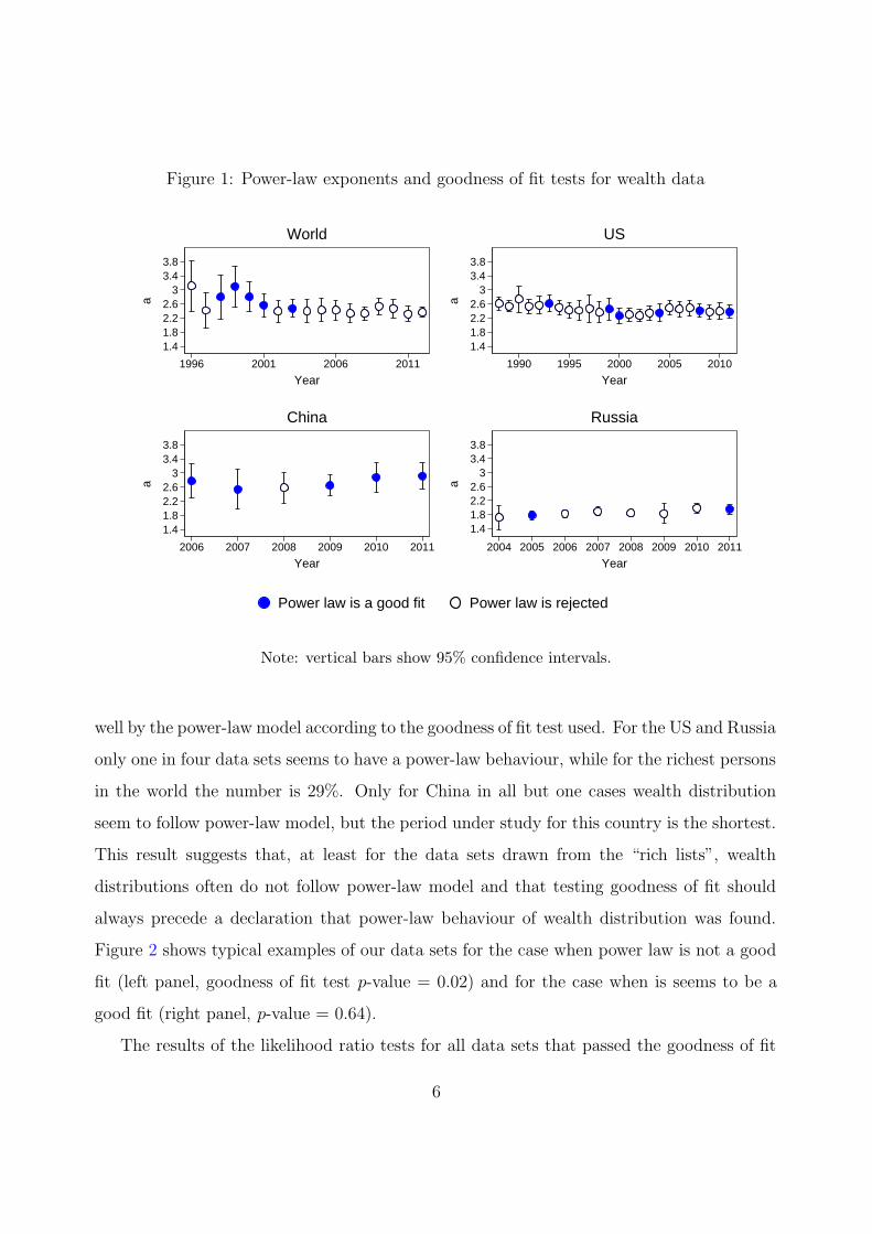
Figure 1: Power-law exponents and goodness of fit tests for wealth data
1.41.82.22.6
33.43.8
a
1996 2001 2006 2011
Year
World
1.41.82.22.6
33.43.8
a
1990 1995 2000 2005 2010
Year
US
1.41.82.22.6
33.43.8
a
2006 2007 2008 2009 2010 2011
Year
China
1.41.82.22.6
33.43.8
a
2004 2005 2006 2007 2008 2009 2010 2011
Year
Russia
Power law is a good fit Power law is rejected
Note: vertical bars show 95% confidence intervals.
well by the power-law model according to the goodness of fit test used. For the US and Russia
only one in four data sets seems to have a power-law behaviour, while for the richest persons
in the world the number is 29%. Only for China in all but one cases wealth distribution
seem to follow power-law model, but the period under study for this country is the shortest.
This result suggests that, at least for the data sets drawn from the “rich lists”, wealth
distributions often do not follow power-law model and that testing goodness of fit should
always precede a declaration that power-law behaviour of wealth distribution was found.
Figure 2 shows typical examples of our data sets for the case when power law is not a good
fit (left panel, goodness of fit test p-value = 0.02) and for the case when is seems to be a
good fit (right panel, p-value = 0.64).
The results of the likelihood ratio tests for all data sets that passed the goodness of fit
6
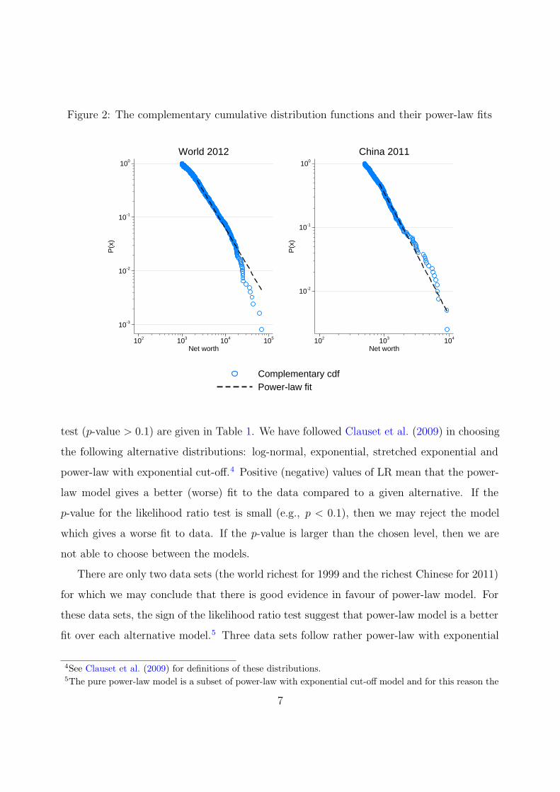
Figure 2: The complementary cumulative distribution functions and their power-law fits
10-3
10-2
10-1
100
P(x
)
102 103 104 105
Net worth
World 2012
10-2
10-1
100
P(x
)
102 103 104
Net worth
China 2011
Complementary cdfPower-law fit
test (p-value > 0.1) are given in Table 1. We have followed Clauset et al. (2009) in choosing
the following alternative distributions: log-normal, exponential, stretched exponential and
power-law with exponential cut-off.4 Positive (negative) values of LR mean that the power-
law model gives a better (worse) fit to the data compared to a given alternative. If the
p-value for the likelihood ratio test is small (e.g., p < 0.1), then we may reject the model
which gives a worse fit to data. If the p-value is larger than the chosen level, then we are
not able to choose between the models.
There are only two data sets (the world richest for 1999 and the richest Chinese for 2011)
for which we may conclude that there is good evidence in favour of power-law model. For
these data sets, the sign of the likelihood ratio test suggest that power-law model is a better
fit over each alternative model.5 Three data sets follow rather power-law with exponential
4See Clauset et al. (2009) for definitions of these distributions.5The pure power-law model is a subset of power-law with exponential cut-off model and for this reason the
7
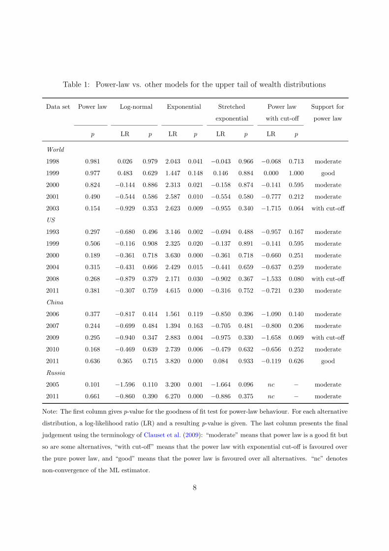
Table 1: Power-law vs. other models for the upper tail of wealth distributions
Data set Power law Log-normal Exponential Stretched Power law Support for
exponential with cut-off power law
p LR p LR p LR p LR p
World
1998 0.981 0.026 0.979 2.043 0.041 −0.043 0.966 −0.068 0.713 moderate
1999 0.977 0.483 0.629 1.447 0.148 0.146 0.884 0.000 1.000 good
2000 0.824 −0.144 0.886 2.313 0.021 −0.158 0.874 −0.141 0.595 moderate
2001 0.490 −0.544 0.586 2.587 0.010 −0.554 0.580 −0.777 0.212 moderate
2003 0.154 −0.929 0.353 2.623 0.009 −0.955 0.340 −1.715 0.064 with cut-off
US
1993 0.297 −0.680 0.496 3.146 0.002 −0.694 0.488 −0.957 0.167 moderate
1999 0.506 −0.116 0.908 2.325 0.020 −0.137 0.891 −0.141 0.595 moderate
2000 0.189 −0.361 0.718 3.630 0.000 −0.361 0.718 −0.660 0.251 moderate
2004 0.315 −0.431 0.666 2.429 0.015 −0.441 0.659 −0.637 0.259 moderate
2008 0.268 −0.879 0.379 2.171 0.030 −0.902 0.367 −1.533 0.080 with cut-off
2011 0.381 −0.307 0.759 4.615 0.000 −0.316 0.752 −0.721 0.230 moderate
China
2006 0.377 −0.817 0.414 1.561 0.119 −0.850 0.396 −1.090 0.140 moderate
2007 0.244 −0.699 0.484 1.394 0.163 −0.705 0.481 −0.800 0.206 moderate
2009 0.295 −0.940 0.347 2.883 0.004 −0.975 0.330 −1.658 0.069 with cut-off
2010 0.168 −0.469 0.639 2.739 0.006 −0.479 0.632 −0.656 0.252 moderate
2011 0.636 0.365 0.715 3.820 0.000 0.084 0.933 −0.119 0.626 good
Russia
2005 0.101 −1.596 0.110 3.200 0.001 −1.664 0.096 nc − moderate
2011 0.661 −0.860 0.390 6.270 0.000 −0.886 0.375 nc − moderate
Note: The first column gives p-value for the goodness of fit test for power-law behaviour. For each alternative
distribution, a log-likelihood ratio (LR) and a resulting p-value is given. The last column presents the final
judgement using the terminology of Clauset et al. (2009): “moderate” means that power law is a good fit but
so are some alternatives, “with cut-off” means that the power law with exponential cut-off is favoured over
the pure power law, and “good” means that the power law is favoured over all alternatives. “nc” denotes
non-convergence of the ML estimator.
8
cut-off model than the pure power-law model, which means that the very highest wealth
observations follow rather exponential than power-law behaviour. However, for each of
these data sets log-normal and stretched exponential models are not ruled out as well. The
remaining majority of data sets give only moderate support for the power-law behaviour in
the sense that some alternatives are also plausible models for these data sets.
In overall, only two out of 55 data sets on wealth distribution analyzed in this paper may
be reliably described as following a pure power-law model. In three cases, power-law with
exponential cut-off seems to be preferred. In 13 cases, power law is not ruled out, but some
other models are also plausible. Among the 37 data sets, which are rejected by the goodness
of fit test, six seem to be better fitted by stretched exponential and 18 by power-law with
cut-off (detailed results not shown for brevity).
These results suggest that the hypothesis that upper tails of wealth distributions, at
least when measured using data from “rich lists”, follow a power-law behavior is statisti-
cally doubtful. It seems obvious that this hypothesis should no longer be assumed without
empirical analysis of a given data using tools similar to those of Clauset et al. (2009). The
existence of popular software implementing such empirical methods should make this task
easier. The results of this paper seem also to cast some doubt on the theoretical literature in
economics and econophysics that provides a theoretical structure for power-law behaviour of
wealth distributions. Theoretical models that make room for some other distributions (espe-
cially power-law with exponential cut-off) describing top wealth values may be empirically
well-founded.
5. Conclusions
In this paper we have used a large number of data sets on wealth distribution taken from
the lists of the richest persons published annually by business magazines like Forbes. Using
former always provides a fit at least as good as the latter. The LR statistic for these models will therefore
be negative or zero. P -values for the data sets with “good” support for power-law behaviour show, however,
that power-law with exponential cut-off are not favoured over pure power-law.
9

recently developed empirical methodology for detecting power-law behaviour introduced by
Clauset et al. (2009), we have found that top wealth distributions follow pure power-law
behaviour only in less than one third of cases. Moreover, even if the data do not rule
out the power-law model, usually the evidence in its favour is not conclusive – some rival
distributions, most notably power law with exponential cut-off, are also plausible fits to
data.
Acknowledgements
I would like to acknowledge gratefully the Matlab and R software written by Aaron Clauset
and Cosma R. Shalizi, which implements methods described in Section 2. The software can
be obtained from http://tuvalu.santafe.edu/˜aaronc/powerlaws/. I also thank Moshe Levy
for sharing data from Forbes 400 Richest Americans lists. All remaining errors are my own.
References
Abul-Magd, A. (2002). Wealth distribution in an ancient Egyptian society. Physical Review E , 66 , 57104.
Aoyama, H., Souma, W., & Fujiwara, Y. (2003). Growth and fluctuations of personal and company’s income.
Physica A: Statistical Mechanics and its Applications , 324 , 352 – 358. Proceedings of the International
Econophysics Conference.
Banerjee, A., Yakovenko, V. M., & Matteo, T. D. (2006). A study of the personal income distribution in
australia. Physica A: Statistical Mechanics and its Applications , 370 , 54 – 59.
Chakrabarti, B., Chakraborti, A., & Chatterjee, A. (Eds.) (2006). Econophysics and sociophysics: trends
and perspectives . Wiley-VCH, Berlin.
Chatterjee, A., Yarlagadda, S., & Chakrabarti, B. (Eds.) (2005). Econophysics of wealth distributions .
Springer Verlag, Milan.
Clauset, A., Shalizi, C. R., & Newman, M. E. J. (2009). Power-law distributions in empirical data. SIAM
Review , 51 , 661–703.
Clementi, F., & Gallegati, M. (2005a). Pareto’s law of income distribution: Evidence for Germany, the
United Kingdom, and the United States. In Chatterjee et al. (2005).
10
Clementi, F., & Gallegati, M. (2005b). Power law tails in the italian personal income distribution. Physica
A: Statistical Mechanics and its Applications , 350 , 427 – 438.
Clementi, F., Matteo, T. D., & Gallegati, M. (2006). The power-law tail exponent of income distributions.
Physica A: Statistical Mechanics and its Applications , 370 , 49 – 53.
Coelho, R., Neda, Z., Ramasco, J., & Augustasantos, M. (2005). A family-network model for wealth
distribution in societies. Physica A, 353 , 515–528.
Dragulescu, A., & Yakovenko, V. (2001). Exponential and power-law probability distributions of wealth and
income in the United Kingdom and the United States. Physica A, 299 , 213–221.
Goldstein, M., Morris, S., & Yen, G. (2004). Problems with fitting to the power-law distribution. The
European Physical Journal B , 41 , 255–258.
Hegyi, G., Nda, Z., & Santos, M. A. (2007). Wealth distribution and pareto’s law in the hungarian medieval
society. Physica A: Statistical Mechanics and its Applications , 380 , 271 – 277.
Jayadev, A. (2008). A power law tail in india’s wealth distribution: Evidence from survey data. Physica A:
Statistical Mechanics and its Applications , 387 , 270 – 276.
Kampstra, P. (2008). Beanplot: A boxplot alternative for visual comparison of distributions. Journal of
Statistical Software , 28 .
Klass, O., Biham, O., Levy, M., Malcai, O., & Solomon, S. (2007). The Forbes 400, the Pareto power-law
and efficient markets. The European Physical Journal B-Condensed Matter and Complex Systems , 55 ,
143–147.
Levy, M. (2003). Are rich people smarter? Journal of Economic Theory , 110 , 42 – 64.
Levy, M., & Solomon, S. (1997). New evidence for the power-law distribution of wealth. Physica A, 242 ,
90–94.
Levy, S. (1998). Wealthy People and Fat Tails: An Explanation for the Lvy Distribution of Stock Returns .
University of California at Los Angeles, Anderson Graduate School of Management 1118 Anderson Grad-
uate School of Management, UCLA.
Ning, D., & You-Gui, W. (2007). Power-law Tail in the Chinese Wealth Distribution. Chinese Physics
Letters , 24 , 2434–2436.
Pareto, V. (1897). Cours d’Economie Politique . F. Rouge, Lausanne.
Richmond, P., Hutzler, S., Coelho, R., & Repetowicz, P. (2006). A review of empirical studies and models
of income distributions in society. In Chakrabarti et al. (2006).
Silva, A., & Yakovenko, V. (2005). Temporal evolution of the” thermal” and” superthermal” income classes
in the USA during 1983-2001. Europhys. Lett , 69 , 304–310.
Sinha, S. (2006). Evidence for power-law tail of the wealth distribution in india. Physica A: Statistical
Mechanics and its Applications , 359 , 555 – 562.
11
Souma, W. (2001). Universal structure of the personal income distribution. Fractals , 9 , 463470.
Vuong, Q. (1989). Likelihood ratio tests for model selection and non-nested hypotheses. Econometrica:
Journal of the Econometric Society , (pp. 307–333).
Yakovenko, V., & Rosser Jr, J. (2009). Colloquium: Statistical mechanics of money, wealth, and income.
Reviews of Modern Physics , 81 , 1703–1725.
Yakovenko, V. M. (2009). Econophysics, statistical mechanics approach to. In R. A. Meyers (Ed.), Ency-
clopedia of Complexity and Systems Science (pp. 2800–2826). Springer, Berlin.
12
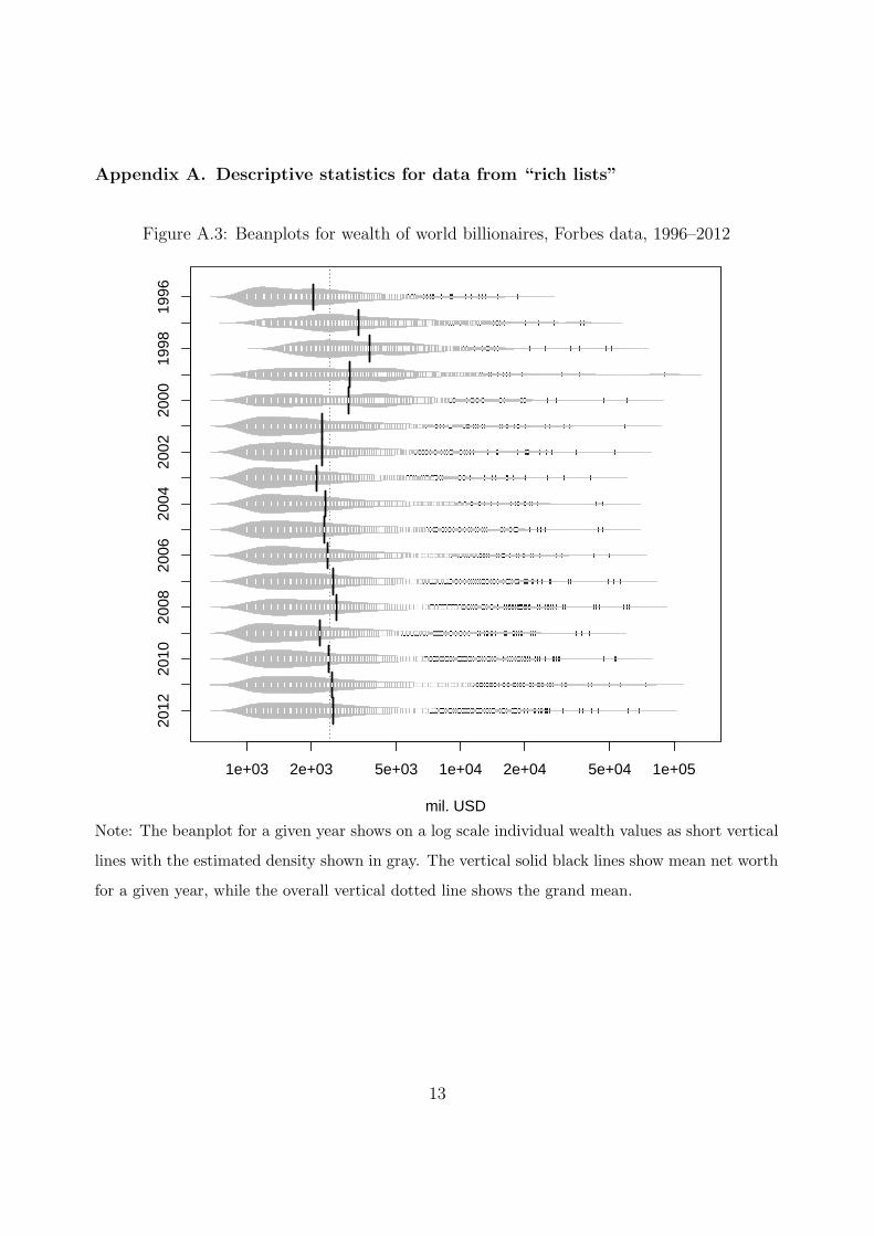
Appendix A. Descriptive statistics for data from “rich lists”
Figure A.3: Beanplots for wealth of world billionaires, Forbes data, 1996–2012
1e+03 2e+03 5e+03 1e+04 2e+04 5e+04 1e+05
2012
2010
2008
2006
2004
2002
2000
1998
1996
mil. USD
Note: The beanplot for a given year shows on a log scale individual wealth values as short vertical
lines with the estimated density shown in gray. The vertical solid black lines show mean net worth
for a given year, while the overall vertical dotted line shows the grand mean.
13
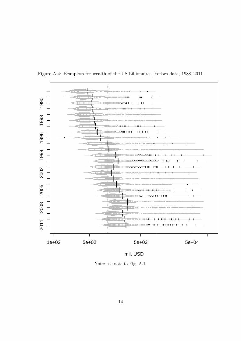
Figure A.4: Beanplots for wealth of the US billionaires, Forbes data, 1988–2011
1e+02 5e+02 5e+03 5e+04
2011
2008
2005
2002
1999
1996
1993
1990
mil. USD
Note: see note to Fig. A.1.
14
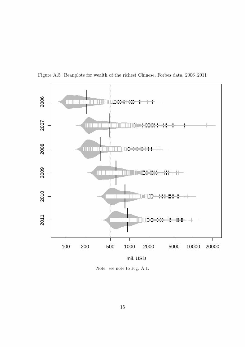
Figure A.5: Beanplots for wealth of the richest Chinese, Forbes data, 2006–2011
100 200 500 1000 2000 5000 10000 20000
2011
2010
2009
2008
2007
2006
mil. USD
Note: see note to Fig. A.1.
15
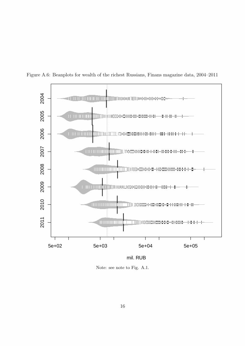
Figure A.6: Beanplots for wealth of the richest Russians, Finans magazine data, 2004–2011
5e+02 5e+03 5e+04 5e+05
2011
2010
2009
2008
2007
2006
2005
2004
mil. RUB
Note: see note to Fig. A.1.
16