boundaries of open marine ecosystems: an application to the pribilof

942

Ecological Applications, 14(3), 2004, pp. 942–953q 2004 by the Ecological Society of America

BOUNDARIES OF OPEN MARINE ECOSYSTEMS: AN APPLICATION TOTHE PRIBILOF ARCHIPELAGO, SOUTHEAST BERING SEA

LORENZO CIANNELLI,1,2,5 BRUCE W. ROBSON,2 ROBERT C. FRANCIS,1 KERIM AYDIN,3

AND RICHARD D. BRODEUR4

1University of Washington, School of Aquatic and Fishery Sciences, Seattle, Washington 98195-5028 USA2National Oceanic and Atmospheric Administration (NOAA), National Marine Mammal Laboratory,

Alaska Fisheries Science Center, 7600 Sand Point Way NE, Seattle, Washington 98115 USA3National Oceanic and Atmospheric Administration (NOAA), Resource Ecology and Fishery Management,

7600 Sand Point Way NE, Seattle, Washington 98115 USA4Northwest Fisheries Science Center, Hatfield Marine Science Center, 2030 South Marine Science Drive,

Newport, Oregon 97365 USA

Abstract. We applied ecosystem energetics and foraging theory to characterize thespatial extent of the Pribilof Archipelago ecosystem, located in the southeast Bering Sea.From an energetic perspective, an ecosystem is an area within which the predatory demandis in balance with the prey production. From a foraging perspective, an ecosystem boundaryshould at least include the foraging range of the species that live within it for a portion oftheir life cycle. The Pribilof Islands are densely populated by species that adopt a centralplace foraging strategy. Foraging theory predicts that the area traveled by central placeforagers (CPF) should extend far enough so that their predatory demands are in balancewith prey production. Thus, the spatial extent of an ecosystem, as defined by energeticsand the foraging range of constituent species, will require a similar energy balance, andindependent assessments should yield similar results. In this study, we compared the areaof maximum energy balance, estimated with a food web model during the decade 1990–2000, with estimates of the foraging range of northern fur seals (the farthest traveling CPFin the Pribilof Islands community) obtained from the literature. From the food web sim-ulations, we estimated that a circle of 100 nautical miles (NM), or 185.2 km, radius enclosesthe area of highest energy balance and lowest biomass import and that it represents a switchfrom a piscivorous-dominated (smaller areas) to a zooplanktivorous-dominated (larger ar-eas) community. The distance from the breeding site to locations recorded at sea for lactatingfemale fur seals, during the years 1995–1996, ranged from 5.0 to 172.2 NM (9.3–318.9km), with a median of 97 NM (179.6 km). Thus, ;50% of the locations recorded forlactating fur seals occurred beyond the area of energy balance estimated by the model,indicating that additional factors can motivate their foraging extent. We propose that en-ergetic constraints set the minimum extent of the Pribilof ecosystem, while the foragingdistance of fur seals may indicate the maximum extent. In discussing these results, wehighlight the limitations of current definitions of the spatial extent in ecosystems, whenrelated to open oceanic environments, and discuss viable alternatives to characterize bound-aries of aquatic systems that are not physically separated from adjacent areas. We believethat these arguments, though controversial, are very timely given the increased emphasiscurrently placed on the management and protection of entire marine ecosystems.

Key words: central place foraging; ecosystem boundary; ecosystem modeling; fur seal; massbalance; Pribilof Islands.

INTRODUCTION

The concept of an ecosystem is central in ecology,however many of its primary attributes, such as thespatial extent, are defined in such a way that limitspractical applicability (Pickett and Cadenasso 2002).A common procedure in ecosystem modeling is that of

Manuscript received 13 January 2003; revised 22 July 2003;accepted 7 August 2003; final version received 15 September2003. Corresponding Editor: A. B. Hollowed.

5 Present address: Centre for Ecological and EvolutionarySynthesis, Department of Biology, University of Oslo, P.O.Box 1050 Blindern, N-0316 Oslo, Norway. E-mail: [email protected]

identifying the spatial extent of an ecosystem withphysical features. For example, the spatial extent ofterrestrial ecosystems can coincide with abrupt changesin topography (e.g., altitude, latitude, exposure), or beenclosed by conspicuous physical barriers, such aslakes, valleys, or canyons. However, similar criteriacompletely fail in marine environments, where mostecosystems have open boundaries, and where areas ofcontrasting hydrography (i.e., fronts) or abrupt topo-graphical discontinuity (i.e., canyons, seamounts, shelfedges) have high productivity and are convergencezones for many different species (Olson et al. 1994,Allen et al. 2001; Genin, in press). Thus, while it is

June 2004 943BOUNDARIES OF OPEN MARINE ECOSYSTEMS

FIG 1. Map of the eastern Bering Sea, with the Pribilof Archipelago. Also shown are the simulated areas in the food webanalysis around the Pribilof Archipelago. Each area has a circular shape with radius of 50, 100, and 150 NM (nautical miles;92.6, 185.2, and 277.8 km, respectively) from a point located at approximately the center of the Pribilof Archipelago (578009000N, 1708009000 W).

clear that the oceans are composed of a mosaic of manyecosystems (Longhurst 1998, Sherman and Duda1999), there exists a lack of supporting theory to spa-tially identify them. This incapacity is particularly se-vere in light of current management practices that placegreater emphasis at the ecosystem level (Griffis andKimball 1996, Botsford et al. 1997, Mooney 1998).There is a need, particularly in marine ecology, to re-define the concept of an ecosystem boundary in sucha way that it meets the distinctiveness of marine en-vironments and can be readily applied for managementpurposes. Here, we attempt to characterize the spatialextent of the ecosystem around the Pribilof Archipel-ago in the southeastern Bering Sea. In the process, wehighlight limitations of current definitions of ecosystemboundaries, when applied to oceanic systems, and dis-cuss viable alternatives.

The Pribilof Archipelago, in the Bering Sea, is com-posed of two larger islands, St. Paul and St. George,and two smaller islands, Walrus and Otter Islands (Fig.1). Despite the absence of defined physical boundaries,the area around the archipelago is ecologically boundedfrom the rest of the Bering Sea. A favorable combi-nation of physical events makes it one of the mostproductive regions in the Bering Sea (Cooney and Coy-le 1982, Coyle and Cooney 1993, Traynor and Smith1996, Flint et al. 2002). High production in the watercolumn permeates to higher trophic levels, in both ben-thic and pelagic systems, and contributes to the for-mation of a unique and abundant community of species.More than 2.5 million seabirds nest and breed on theislands during the summer months, including Thick-billed Murres (Uria lomvia), Common Murres (Uriaaalge), Red-legged Kittiwakes (Rissa brevirostris),

944 LORENZO CIANNELLI ET AL. Ecological ApplicationsVol. 14, No. 3

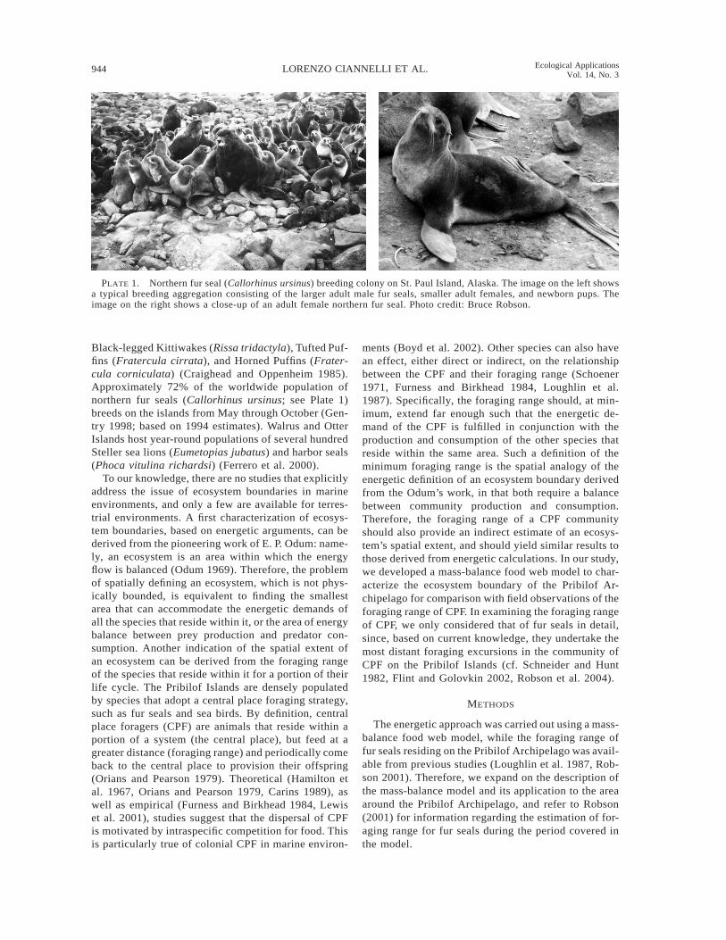
PLATE 1. Northern fur seal (Callorhinus ursinus) breeding colony on St. Paul Island, Alaska. The image on the left showsa typical breeding aggregation consisting of the larger adult male fur seals, smaller adult females, and newborn pups. Theimage on the right shows a close-up of an adult female northern fur seal. Photo credit: Bruce Robson.

Black-legged Kittiwakes (Rissa tridactyla), Tufted Puf-fins (Fratercula cirrata), and Horned Puffins (Frater-cula corniculata) (Craighead and Oppenheim 1985).Approximately 72% of the worldwide population ofnorthern fur seals (Callorhinus ursinus; see Plate 1)breeds on the islands from May through October (Gen-try 1998; based on 1994 estimates). Walrus and OtterIslands host year-round populations of several hundredSteller sea lions (Eumetopias jubatus) and harbor seals(Phoca vitulina richardsi) (Ferrero et al. 2000).

To our knowledge, there are no studies that explicitlyaddress the issue of ecosystem boundaries in marineenvironments, and only a few are available for terres-trial environments. A first characterization of ecosys-tem boundaries, based on energetic arguments, can bederived from the pioneering work of E. P. Odum: name-ly, an ecosystem is an area within which the energyflow is balanced (Odum 1969). Therefore, the problemof spatially defining an ecosystem, which is not phys-ically bounded, is equivalent to finding the smallestarea that can accommodate the energetic demands ofall the species that reside within it, or the area of energybalance between prey production and predator con-sumption. Another indication of the spatial extent ofan ecosystem can be derived from the foraging rangeof the species that reside within it for a portion of theirlife cycle. The Pribilof Islands are densely populatedby species that adopt a central place foraging strategy,such as fur seals and sea birds. By definition, centralplace foragers (CPF) are animals that reside within aportion of a system (the central place), but feed at agreater distance (foraging range) and periodically comeback to the central place to provision their offspring(Orians and Pearson 1979). Theoretical (Hamilton etal. 1967, Orians and Pearson 1979, Carins 1989), aswell as empirical (Furness and Birkhead 1984, Lewiset al. 2001), studies suggest that the dispersal of CPFis motivated by intraspecific competition for food. Thisis particularly true of colonial CPF in marine environ-

ments (Boyd et al. 2002). Other species can also havean effect, either direct or indirect, on the relationshipbetween the CPF and their foraging range (Schoener1971, Furness and Birkhead 1984, Loughlin et al.1987). Specifically, the foraging range should, at min-imum, extend far enough such that the energetic de-mand of the CPF is fulfilled in conjunction with theproduction and consumption of the other species thatreside within the same area. Such a definition of theminimum foraging range is the spatial analogy of theenergetic definition of an ecosystem boundary derivedfrom the Odum’s work, in that both require a balancebetween community production and consumption.Therefore, the foraging range of a CPF communityshould also provide an indirect estimate of an ecosys-tem’s spatial extent, and should yield similar results tothose derived from energetic calculations. In our study,we developed a mass-balance food web model to char-acterize the ecosystem boundary of the Pribilof Ar-chipelago for comparison with field observations of theforaging range of CPF. In examining the foraging rangeof CPF, we only considered that of fur seals in detail,since, based on current knowledge, they undertake themost distant foraging excursions in the community ofCPF on the Pribilof Islands (cf. Schneider and Hunt1982, Flint and Golovkin 2002, Robson et al. 2004).

METHODS

The energetic approach was carried out using a mass-balance food web model, while the foraging range offur seals residing on the Pribilof Archipelago was avail-able from previous studies (Loughlin et al. 1987, Rob-son 2001). Therefore, we expand on the description ofthe mass-balance model and its application to the areaaround the Pribilof Archipelago, and refer to Robson(2001) for information regarding the estimation of for-aging range for fur seals during the period covered inthe model.


Food web ecosystem model

The energy balance between predator demand andprey availability was estimated using a mass-balanceanalysis on different geographic scales, each represen-tative of a progressively larger concentric region withthe Pribilof Archipelago at its center. Our fundamentalassumption was that the smallest system reaching en-ergetic balance was representative of the ecosystemboundary. The model used to calculate the energy flowwithin a community was ECOPATH (Polovina 1984,Christensen and Pauly 1992, Christensen et al. 2000),distributed online by the Fisheries Centre at the Uni-versity of British Columbia, British Columbia, Cana-da.6 Henceforth, we briefly reiterate the main charac-teristics of the model structure, and emphasize the ma-jor aspects of relevance to this study.

ECOPATH is a static mass-balance model that de-scribes the flow of energy within a trophic web. Assum-ing a mass balance and a steady state, the productionfrom a trophic group i, is partitioned as follows:

n

P 5 Q 1 Ex 1 L (1)Oi i j i ij51

where Pi indicates production of group i and is cal-culated as the product of the production to biomassratio (P/Bi) and biomass (Bi),

P 5 (P/B )B .i i i

Qij indicates the consumption by predator j of prey iand is calculated as the product of the fraction of preyi in the diet of predator j (diet composition, DCij), thepredator consumption to biomass ratio (Q/Bj), and thepredator biomass (Bj):

Q 5 DC (Q/B )B .ij ij j j

Li indicates the amount of production of group i thatis left over after predation (Qij) and export or fishing(Exi). In ECOPATH, Li is calculated as the productbetween production and 1 minus the ecotrophic effi-ciency (EEi):

L 5 (1 2 EE ) 3 (P/B ) 3 B .i i i i

EEi is the fraction of production that remains in thesystem (i.e., depredated) or is removed by fishing. Bysubstitution into Eq. 1 and rearranging,

n

(P /B )B EE 5 Ex 2 DC (Q /B )B (2)Oi i i i ji j jj51

where n is the total number of trophic groups includedin the model.

In ECOPATH, the total mortality fraction of a group(Z ) is composed of predation mortality (M2), fishingmortality (F), and ‘‘other mortality’’ (M0) due to dis-eases or senescence. For each group, the three sourcesof mortality are derived as follows:

6 URL: ^www.ecopath.org&

QO i jj

M2 5 (3)i Bi

HiF 5 (4)i Bi

where Hi is harvest on group i,

M0 5 (1 2 EE )Z . (5)i i i

Moreover, for each group, M2 is further partitionedamong all predators that feed on it, in proportion tothe quantity consumed (Christensen et al. 2000).

In this application, Eq. 2 is solved for EE, and theinput parameters for each trophic group included in thefood web are P/B (yr21), Q/B (yr21), B (Mg/km2), anddiet composition (DC) expressed as weight fractions.If group production does not exceed the amount pre-dated upon or removed, then the EE will be less thanor equal to 1. However, if production is lower thanpredation or removal, then the EE will be higher than1, in proportion to the amount needed to fulfill theexcess that is lost.

Trophic groups and parametersof the food web model

This analysis focused on the decade 1990–2000. Atotal of 39 trophic groups plus two detritus pools (ben-thic and pelagic) were included in the ECOPATH rep-resentation of the Pribilof Islands food web (Table 1).The characterization of a trophic group was based ondifferent criteria, including the relative abundance,similarities in physiology, and diet among species. Tro-phic groups that can potentially follow a CPF feedingstrategy were fur seals, Steller sea lions, Common andThick-billed Murres, Red- and Black-legged Kitti-wakes, Horned and Tufted Puffins, and Red-faced Cor-morants. A detailed description of the parameterizationof each trophic group (i.e., determination of biomass,P/B and Q/B, and diet) is presented in the Appendix.

Food web simulations

We estimated the energetic balance of three trophicwebs, each representative of a species assemblage atincreasing distances from the Pribilof Islands. Theshape of each simulated area was assumed to be a cir-cle, with radii of 50 nautical miles (NM) (92.6 km; 50-NM system), 100 NM (185.2 km; 100-NM system),and 150 NM (277.8 km; 150-NM system) from a pointlocated at approximately the center of the Pribilof Ar-chipelago (57800.009 N, 170800.009 W; Fig. 1). Foreach trophic group, the balance between predator de-mand and prey availability was measured by the EE ofthe prey (i.e., EE . 1 indicated that more prey biomasswas removed than produced). The total mortality rate(Z ) of groups with EE . 1 (henceforth overtaxedgroups) was partitioned among its component M2, F,and M0, using Eqs. 3, 4, and 5, respectively. Moreover,


TABLE 1. List of trophic groups included in food web analysis, with respective trophic level (TL), production to biomassrate (P/B, yr21), consumption to biomass rate (Q/B, yr21), and biomass (B, Mg/km2).

Trophic group Description TL P/B Q/B

Biomass (Mg/km2)

50 NM 100 NM 150 NM

Phytoplankton diatoms: Thalassiosira spp., Chae-toceros spp.

1 148.10 ··· 36.22 36.22 36.22

Pelagic detritus 1 ··· ··· ··· ··· ···Benthic detritus 1 ··· ··· ··· ··· ···Protozoa phytoflagelates, semi-autotrophic 1.5 72.00 144.00 10.00 10.00 10.00Bacterioplankton 2 150.00 300.00 11.08 11.08 11.08Crabs Chionoecetes opilio, Paralithodes

spp.2 1.16 5.09 1.78 1.48 1.27

Infauna bivalves, polychaetes, benthic am-phipods

2 1.97 12.00 22.45 17.99 13.83

Mesozooplankton copepods: Calanus marshallae,Neocalanus spp.

2.2 9.00 27.00 25.74 25.74 25.74

Microzooplankton ciliates, nauplii, trocophores, veli-gers

2.2 9.00 27.00 13.26 13.26 13.26

Macrozooplankton euphausiids: Thysanoessa spp., Eu-phausia pacifica

2.4 2.70 9.00 16.60 16.60 16.60

Epibenthic seastars, sponges, pagurids 2.6 1.57 5.78 6.99 5.81 4.39Small jellies hydromedusae, larvaceans: Oiko-

pleura2.6 7.00 23.00 50.00 50.00 50.00

Agonidae Podothecus acipenserinus, Sarritorfrenatus

3.1 0.40 2.56 0.13 0.07 0.05

Small flatfishes Lepidosetta polyxystera, Limandaaspera

3.1 0.40 2.97 8.12 7.05 5.47

Chaetognaths Sagitta elegans 3.2 1.35 3.87 25.05 25.05 25.05Forage fishes Clupea pallasii, Mallotus villosus 3.3 1.00 7.00 0.01 5.00 10.00Liparidae Careproctus spp. 3.4 0.60 2.49 ,0.01 0.01 0.02Mesopelagic fishes Bathylagus, Leuroglossus, Steno-

brachius3.4 1.57 7.83 ,0.01 1.48 2.20

Zoarcidae Bothrocara brunneum, Lycodesspp.

3.4 0.60 2.49 0.06 0.23 0.28

Juvenile gadids Theragra chalcogramma, Gadusmacrocephalus

3.5 6.97 20.23 1.37 1.40 1.34

Rockfishes Sebastes alutus, S. borealis, S.alascanus

3.5 0.16 3.10 0.08 1.24 2.77

Grenadiers Albatrossia pectoralis, Coryphae-noides cinereus

3.6 0.40 2.49 ,0.01 12.87 13.83

Adult pollock Theragra chalcogramma 3.7 0.50 4.16 15.60 11.66 8.56Large jellies Chrysaora melanaster 3.8 1.50 3.00 15.00 16.00 19.00Sculpins Hemilepidotus spp., Hemitripterus

bolini3.8 0.40 2.56 0.98 0.61 0.48

Squids Berryteuthis magister and Gonatusspp.

3.8 3.20 10.67 1.00 2.00 3.50

Skates Bathyraja spp. 3.9 0.40 2.56 1.04 1.03 1.11Thick-billed Murres Uria lomvia 3.9 0.97 33.31 0.05 0.01 0.01Adult cod Gadus macrocephalus 4 0.50 4.16 2.42 1.86 1.43Large flatfishes Atherestes stomias, Hippoglossus

stenolepis4.1 0.40 2.92 2.83 2.99 3.03

Black-legged Kittiwakes Rissa tridactyla 4.2 0.80 32.15 ,0.01 ,0.01 ,0.01Steller sea lions Eumetopias jubatus 4.2 0.06 27.04 ,0.01 ,0.01 ,0.01Puffins Fratercula spp. 4.3 0.80 23.50 ,0.01 ,0.01 ,0.01Red-legged Kittiwakes Rissa brevirostris 4.3 0.80 20.72 ,0.01 ,0.01 ,0.01Sablefish Anoplopoma fimbria 4.3 0.40 2.49 ,0.01 0.13 0.20Common Murre Uria aalge 4.4 1.09 29.14 0.02 ,0.01 ,0.01Harbor seals Phoca vitulina richardsi 4.4 0.06 19.44 ,0.01 ,0.01 ,0.01Red-faced Cormorant Phalacrocorax urile 4.4 0.80 18.89 ,0.01 ,0.01 ,0.01Dall porpoises Phocoenoides dalli 4.5 0.40 2.56 ,0.01 0.07 0.17Fur seals Callorhinus ursinus 4.6 0.06 19.96 1.30 0.32 0.14Sleeper sharks Somniosus pacificus 4.6 0.06 28.01 ,0.01 ,0.01 ,0.01

Notes: The biomass is shown for each system (50 NM, 100 NM, 150 NM) simulated (NM 5 nautical miles; 1 NM 51.852 km).

to evaluate the deficit of production of the overtaxedgroup, we calculated the amount of biomass needed tobalance the predator–prey trophic link: Preq 5 EE 3 B3 (P/B). The difference between the realized (P) and

the required production (Preq) is indicative of theamount of extra biomass that is needed from outsidethe system, in order to balance the food web (i.e., thebiomass import).


TABLE 2. Factors used to determine the parameter distri-bution to estimate EB error.

Group

Parameter range

Biomass P/B Q/B Diet

PhytoplanktonPelagic detritusBenthic detritusProtozoaBacterioplankton

0.1······0.50.5

0.1······0.30.3

·········0.30.3

·········

0.30.3

CrabsInfaunaMesozooplanktonMicrozooplanktonMacrozooplankton

0.10.80.10.80.5

0.40.50.20.30.2

0.40.60.20.30.2

0.30.30.30.30.3

EpibenthicSmall jelliesAgonidaeSmall flatfishesChaetognaths

0.10.50.10.10.1

0.40.40.40.40.2

0.40.40.40.40.2

0.30.30.30.30.3

Forage fishesLiparidaeMesopelagic fishesZoarcidaeJuvenile gadids

0.80.10.80.80.1

0.40.40.40.40.2

0.40.40.40.40.2

0.30.30.30.30.1

RockfishesGrenadiersAdult pollockLarge jelliesSculpins

0.10.10.10.10.1

0.40.40.20.40.4

0.40.40.20.40.4

0.30.30.30.30.3

SquidsSkatesThick-billed MurresAdult codLarge flatfishes

0.80.10.10.10.1

0.50.40.40.40.4

0.60.40.40.40.4

0.30.30.30.30.3

Black-legged KittiwakesSteller sea lionsPuffinsRed-legged KittiwakesSablefish

0.10.10.10.10.1

0.40.40.40.40.4

0.40.40.40.40.4

0.30.30.30.30.3

Common MurreHarbor sealsRed-faced CormorantDall porpoises

0.10.10.10.1

0.40.40.40.4

0.40.40.40.4

0.30.30.30.3

Fur sealsSleeper sharks

0.10.1

0.40.4

0.40.4

0.30.3

Note: The sampling range around each parameter is drawnfrom a uniform distribution whose upper and lower extremesare specified by the initial parameter estimate multiplied bythe factors listed in the table.

FIG. 2. Food consumption (Mg·km22·yr21) of all groupswith trophic level . 4, resulting from a food web analysisfor each of the three simulated systems (50 NM, 100 NM,and 150 NM). ‘‘Other MM’’ refers to marine mammals otherthan fur seals.

To evaluate the degree of energy balance at an overallecosystem level, we defined a unique metric, EB, fromthe sum of the EEs of the overtaxed groups only:

m

EB 5 EE (6)O kk51

where m is the number of overtaxed groups within asimulated system. Using a Monte Carlo resampling ap-proach, we assessed the error of EB estimates from1000 model runs generated by random combinationsof input parameters sampled from prespecified uniformdistributions (Table 2). The parameter distributionsused in the error analysis were representative of theuncertainty in the initial parameter estimate. In esti-mating the error around EB, the EE of fishes in thefamily Zoarcidae was set to 0.9 under the assumption

that the unbalance of this trophic group was the resultof low catchability rather than excess predation or re-moval (see Discussion). Differences between estimatedEB were statistically tested by ANOVA on log-trans-formed data (EB were not normally distributed). If themain factor effect was found significant at 95% con-fidence, we proceeded to detect group mean differencesusing Bonferroni-adjusted pairwise comparisons.

RESULTS

Groups that had the greatest change in biomass asthe boundary was increased from the 50- to the 150-NM system were the CPF assemblage; the species typ-ically found along the slope community and the foragefish assemblage. CPF biomass, primarily driven by furseals, decreased by approximately one order of mag-nitude, corresponding to the increase in area betweenthe 50- and the 150-NM system (Table 1). In contrast,taxa generally associated with the slope communityincreased in biomass by several orders of magnitude,which would be expected since the slope area was ex-cluded from the 50-NM system. The dominant slopegroups were grenadiers and mesopelagic fishes, with alower contribution by sleeper sharks, liparids, sablefishand rockfish (Table 1). Forage fish also increased inbiomass over larger boundaries, but their center of dis-tribution was to the north and east of the Pribilof Is-lands rather than along the slope.

Based on their diet, fur seals and sleeper sharks hadthe highest trophic level (TL 5 4.6) of all the groupssimulated. Within the 50-NM system, fur seals largelydominated the biomass and total food consumption ofCPF; seabird consumption summed to 2.26 Mg·km22·yr21, consumption by other marine mammals summedto 0.08 Mg·km22·yr21 and fur seal consumption was26.00 Mg·km22·yr21. If fur seal consumption was stan-dardized for the loss of energy among trophic levels(transfer efficiency), then it would be the largest of all


TABLE 3. Results of ecotrophic efficiency (EE) for all tro-phic groups and ecosystem areas (50 NM, 100 NM, and150 NM) simulated.

Group name

Ecotrophic efficiency

50 NM 100 NM 150 NM

PhytoplanktonPelagic detritusBenthic detritusProtozoaBacterioplankton

0.410.600.110.860.19

0.410.600.090.860.19

0.410.610.080.860.19

CrabsInfaunaMesozooplanktonMicrozooplanktonMacrozooplankton

1.240.900.602.421.55

1.400.900.742.421.80

1.520.900.882.422.14

EpibenthicSmall jelliesAgonidaeSmall flatfishes

0.630.013.440.36

1.420.012.110.28

1.970.022.680.46

ChaetognathsForage fishesLiparidaeMesopelagic fishes

0.141387.31

0.164198.11

0.141.140.163.67

0.140.610.162.82

ZoarcidaeJuvenile gadidsRockfishesGrenadiersAdult pollock

16.293.310.220.623.09

44.953.230.020.622.23

41.143.680.020.622.45

Large jelliesSculpinsSquidsSkatesThick-billed Murres

0.000.694.890.040.00

0.000.712.230.060.00

0.000.701.220.030.00

Adult codLarge flatfishesBlack-legged KittiwakesSteller sea lions

0.660.840.000.00

0.350.740.000.00

0.270.710.000.00

PuffinsRed-legged KittiwakesSablefishCommon MurreHarbor sealsRed-faced CormorantDall porpoises

0.000.000.000.000.000.000.00

0.000.000.000.000.000.000.00

0.000.000.000.000.000.000.00

Fur sealsSleeper sharks

0.030.00

0.030.00

0.030.00

Note: Groups with EE . 1 are in boldface. NM 5 nauticalmile. 1 NM 5 1.852 km.

groups simulated in the 50-NM system. Within the 50-NM boundary, fur seal consumption also dominatedamong groups with TL . 4, which besides the CPFincluded sleeper sharks, large flatfishes, harbor seals,Dall’s porpoises, and sablefish (Fig. 2). However, asthe area was increased from the 50- to 150-NM system,fur seal and CPF food consumption decreased propor-tionally and became lower than that of non-CPF groups(Fig. 2).

Within the 50-NM system, many species were inenergetic imbalance, as suggested by their high EE(Table 3). Trophic groups with highest EE were me-sopelagic fish (EE 5 4198.11) and shelf forage fish(EE 5 1387.31). Other overtaxed groups were zoar-cidae, adult pollock, agonids, juvenile gadids, squids,macrozooplankton, microzooplankton, and crabs (Ta-ble 3). Fur seals caused more than 76% and 42% of

the total predation mortality of the mesopelagic andshelf forage fishes, respectively (Fig. 3). Increasing thesystem boundary from 50 to 100 NM (from 92.6 to185.2 km) substantially reduced the energetic imbal-ance of mesopelagic and shelf forage fishes. Their re-spective EE dropped to 3.67 and 1.14 (Table 3). Otherovertaxed groups that had a decrease in EE in the 100-NM system were adult pollock (3.09 to 2.23), squids(4.89 to 2.23), agonids (3.44 to 2.11), and juvenilegadids (3.31 to 3.23). Some overtaxed groups furtherincreased their EE from the 50- to the 100-NM system.These were zoarcids (from 16.29 to 44.95), macrozoo-plankton (from 1.55 to 1.80), crabs (from 1.24 to 1.40),and epibenthic fauna (from 0.63 to 1.42) (Table 3). Afurther increase of the system boundary, from the 100-to 150-NM system resulted in a further energetic bal-ance of mesopelagic fishes, forage fishes, and squids,albeit to a much smaller degree than that observed fromthe 50- to the 100-NM system (Table 3). However, alarger number of trophic groups further increased theirEE in the 150-NM simulation with respect to the 100-NM simulation. These were adult pollock, agonids,macrozooplankton, crabs, epibenthic, and juvenile gad-ids. Zoarcids, which had initially increased their EEfrom the 50- to the 100-NM systems, decreased in theirEE for the 150-NM system (Table 3).

The estimated average EB for each system, resultingfrom the Monte Carlo model run under parameter un-certainty, was 8349.49 (1 SD 5 5252.89) for the 50-NM system, 22.57 (6.42) for the 100-NM system and25.34 (7.14) for the 150-NM system (Fig. 4). All EBvalues were significantly different from each other(Bonferroni, P , 0.001). It is important to note thatnone of the simulated areas reached a balance betweenprey production and predator consumption. From themodel simulations it appeared that the 100-NM systemrequired the lowest import in order to reach the balance,while the 150-NM system required the highest (Table4). The import of zooplankton biomass (including mi-cro- and macro-zooplankton) increased with the in-crease of the ecosystem boundary, while the import offish biomass (including pollock, forage, mesopelagic,juvenile gadids, and squids) decreased (Table 4). Thispattern indicates that there was an excess of piscivoryin the 50-NM system and an excess of zooplanktivoryin the 150-NM system.

DISCUSSION

Our analysis clearly showed that within 50 NM (92.6km) of the center of the Pribilof Islands the predatorydemand is unsustainable, given the available prey bio-mass and production. However, an enlargement of theecosystem boundary can bring the predator communitytoward a better energetic balance with their prey. Thiswas indicated by a progressive reduction of the EE ofovertaxed groups (Table 3), by a reduction of whole-system EB (Fig. 4), and by a reduction of the requiredbiomass import (Table 4). Key prey species in defining


FIG. 3. Partitioning of predation mortality (M2) of all groups with EE . 1 in the 50-NM ecosystem simulation. Preygroups are indicated in the x-axis, and predator groups are identified in the key (zooplankton 5 micro-, meso-, and macro-zooplankton; other MM 5 marine mammals other than fur seals). Abbreviations for x-axis: macrozp. 5 macrozooplankton;microzp. 5 microzooplankton; juv. gadids 5 juvenile gadids.

FIG. 4. Natural logarithm of average energy balance (EB)from 1000 model simulations of each system, based on ran-dom combinations of input parameters sampled from pre-specified uniform distributions (see Table 2). Error bars are6 1SD.

TABLE 4. Estimates of biomass import (Mg·km22·yr21) foreach overtaxed trophic group and simulated ecosystemarea.

Group name 50 NM 100 NM 150 NM

Adult pollockZooplanktonAll forageAll epibenthicAgonidae

16.27194.40

49.410.500.12

7.19205.69

36.134.620.03

6.21220.80

33.737.550.03

Sum 260.69 253.66 268.31

Notes: Zooplankton 5 micro- and macrozooplankton; allforage 5 mesopelagic, forage, juvenile gadids, and squids;all epibenthic 5 epibenthic and crabs. Zoarcidae, althoughovertaxed, were not included in the calculation of biomassimport. NM 5 nautical mile. 1 NM 5 1.852 km.

the community energetic balance were the mesopelagicfishes and shelf forage fishes, and the key predatorspecies were the CPF, in particular, fur seals. Both adispersion of fur seal predation over a broader area andan inclusion of more forage and mesopelagic fish bio-mass within the modeled area moved the system towardenergetic balance with boundary enlargement. About32% of the fur seal diet depended on shelf forage andmesopelagic fishes, which were almost completely ex-cluded within the 50-NM boundary system. Mesope-lagic fishes tended to be more abundant toward the shelfbreak (Sinclair et al. 1999, Sinclair and Stabeno 2002).Likewise, shelf-forage species, other than juvenile gad-

ids, were more abundant toward the northern and east-ern part of the shelf (Brodeur et al. 1999, Nebenzahland Goddard 2000).

The achievement of energetic balance between pred-ator demand and prey availability, however, did notprogress steadily as the system increased its boundary,as shown by some of the metrics developed in thisstudy. In fact, the system EB and biomass importreached a minimum at the 100-NM area. Also, the typeof import switched from primarily fish (50-NM system)to primarily zooplankton (150-NM system), indicatingthat the 100-NM area was in balance between piscivory(high in the 50-NM system) and zooplanktivory (highin the 150-NM system). Thus, while the Pribilof systemgained energetic balance upon an initial boundary en-largement (from 50 to 100 NM), a further enlargementdid not result in more stability, but rather brought the


system toward new imbalances and an excess of zoo-planktivory. These results indicate that the Pribilof eco-system boundary cannot grow indefinitely, further cor-roborating the assumption of a functional distinctionof the Pribilof area from the rest of the Eastern BeringSea. We therefore conclude that, during the decade1990–2000, the 100-NM simulation yielded a more re-alistic representation of a minimum area required fora balanced trophic web than both the 50-NM and the150-NM simulations.

Within the proposed area of energy balance, how-ever, there were still several energetically unbalancedgroups. The majority of them were either planktonicorganisms, such as macrozooplankton, microzooplank-ton and juvenile gadids, or migrating demersal and for-age fish, such as age 11 pollock. One other group thatdid not fit in either category and yet was unbalancedwas zoarcid fishes (i.e., eelpouts), with the highest EEamong all groups in the 100-NM system (Table 3). Withrespect to planktonic or migrating demersal and foragefish, the unbalances could actually reflect a net importof biomass from adjacent areas into the Pribilof eco-system. Biomass import was not included in our modeldue to the lack of studies that could support any rea-sonable estimate of such a quantity. However, we wereable to estimate that the amount of import required tobalance each simulated food web minimized at the 100-NM area (Table 4). The role of net biomass import inthe characterization of open-boundary marine ecosys-tems is considered in the Discussion.

With respect to zoarcids, the imbalance in each ofthe simulated Pribilof areas could reflect a low catch-ability of the sampling gear for this taxon. In the easternBering Sea, there is no direct fishery on zoarcids andconsequently there is little incentive to improve theirbiomass estimates. However, zoarcid fishes play an im-portant role both as predator and prey, especially incommunities associated with the shelf edge, where theirabundance typically peaks. In the Pribilof ecosystem,for example, zoarcids occurred in the diet of manyabundant demersal fish, such as grenadiers, adult pol-lock, large flatfishes, and skates (Appendix; Brodeurand Livingston 1998), and yet their biomass, estimatedfrom trawl survey, was not sufficient to sustain thepredatory demand by at least one order of magnitude.Similar results were obtained for the entire Bering Seaecosystem (Aydin et al. 2002) and the Northern Cali-fornia Current ecosystem (Field et al. 2001).

The dominant CPF species in the model, northernfur seals, did not limit their foraging to the minimumarea required (100 NM) for energetic balance. Duringforaging trips (N 5 119) made by lactating fur seals(N 5 97) in 1995–1996, the median distance from thebreeding site to locations recorded at sea was 97.0 NM(179.6 km) on average (range 5.0 to 172.2 NM (9.3 to318.9 km), 1 SD 5 32.1 NM (59.4 km); Robson 2001).Some of this discrepancy is attributable to the differ-ence between distance measurements made from in-

dividual breeding sites and the central point used forthe 50-, 100-, and 150-NM radii (92.6, 185.2, and 277.8km) in the ECOPATH model. However, the magnitudeof this difference was small (mean 5 16.7 NM [30.9km], range 5 0.4–29.1 NM [0.7–53.9 km], 1 SD 5 8.8NM [16.3 km]) relative to the distance females traveledfrom the islands. Furthermore, the maximum distancerecorded for the same foraging trips exceeded 240 NM(444.5 km) with a mean of 130.4 NM (241.5 km) (Rob-son 2001). Thus, ;50% of the at-sea locations recordedfor satellite-tracked females in 1995–1996 were beyondthe minimum area of energy balance (100 NM [185.2km]) estimated in our study. In addition, male fur seals,which constitute ;30% of the non-pup biomass of thePribilof Island population (Lander 1981), travel furtherfrom the breeding islands than lactating fur seals(Loughlin et al. 1999; National Marine Fisheries Ser-vice, unpublished data). Clearly, additional factors, be-sides that of reaching an area with sufficient energybalance, motivate the dispersal of fur seals during theirforaging trips. Below we list and discuss some of thesefactors as they can provide important insight into theactual spatial extent required for energetic balancewithin an ecosystem.

Location, density, and species composition of preyshould influence the foraging range of fur seals. TheECOPATH model shows that fur seals exert a massivepredatory impact on the Pribilof system. This result isin accordance with predictions made more than 30years ago by Laevastu et al. (1976) for the Bering Sea.Similarly, Boyd et al. (2002) and Boyd (2002) foundthat lactating Antarctic fur seals (Arctocephalus ga-zella) likely have a dominant role among top predatorsforaging in waters surrounding South Georgia. FemaleAntarctic fur seals consume one-tenth of the mean den-sity of krill on average and could eat almost all of thekrill present in regions of intense foraging. Given theirlarge impact, fur seals and other marine predators likelyfeed on high-density aggregations of prey in order tomaximize their net energy gain relative to foragingcosts. The ECOPATH model, however, assumes a uni-form spatial and temporal distribution of biomass with-in each modeled area, while, in reality, production ispulsed and prey are patchily distributed (e.g., Swartz-man and Hunt 2000). In addition, a greater proportionof high-density patches might be located outside a giv-en area of energy balance in a particular year or season.In a patchy prey environment, an optimal central placeforaging strategy may be to travel directly to an areaof high prey concentration where predators search ran-domly for prey, thereby increasing the encounter rateof prey patches per unit of area searched (Orians andPearson 1979, Schoener 1971). Linear, directed move-ments away from colonies have been documented inseveral fur seal species (Boyd et al. 1998, Bonadonnaet al. 2001, Robson et al. 2004) and may facilitate theability of individual animals to return to productiveforaging areas. While such directed movements away


from the central place may reduce predator impact dueto the effect of geometric spreading, they are also likelyto increase the relative dispersal distance if predictableareas of high prey density are located further from thebreeding colony in some years.

In addition to prey patchiness, fur seal dispersal maybe regulated by a preference for larger or more nutri-tional forage fishes (e.g., mesopelagic species, herring,capelin, or eulachon), or alternatively by a preferencefor adult over juvenile pollock. Both the forage speciesand adult pollock have higher energy and fatty acidcontent than age-0 pollock (Van Pelt et al. 1997, Cian-nelli et al. 2002), and are less abundant than age-0pollock within the 50-NM boundary. Recent stable iso-tope analyses indicate that during the fall lactating furseals eat prey at trophic levels equivalent to 2–4-yr-old walleye pollock and small Pacific herring (Kurleand Worthy 2001, 2002). While isotopic ratios did notindicate a diet dominated by juvenile pollock, a com-bined diet of older pollock mixed with juvenile pollockand other species (e.g., squid) would fall within therange of nitrogen isotope values observed (Kurle andWorthy 2002). These studies, in conjunction with ourECOPATH simulations, support theoretical predictionsthat larger or more nutritious prey are more likely tobe favored as foraging distance increases (Schoener1971, Orians and Pearson 1979).

In considering the results of this study, it is importantto take into account the degree of uncertainty that wentinto parameterization of the ECOPATH model (Ap-pendix). The relative level of uncertainty of the modelparameters is proportional to the coefficients shown inTable 2. In general, the biomass of the forage com-ponents, including squids, forage fishes, and mesope-lagic fishes, was the most uncertain, unlike those ofgroundfish and CPF species. Also, the diet of fur sealswas influenced by information from scat collections;hence, it might over-represent prey eaten during thelast meals of a foraging trip. Although the assumptionsmade in parameterizing the food model can certainlyinfluence the energy balance of a predator–prey trophiclink, the estimated pattern of the EB metric across thethree simulated areas, on which we based our assess-ment of highest energy balance, was robust to a widerange of uncertainty. As more precise data becomeavailable for constituent species in the Pribilof eco-system, examining the sensitivity of energetic balanceat a broader range, finer scale of spatial resolution, anddifferent (i.e., not circular) ecosystem shapes could re-fine our analysis.

Our study and the methodology applied bring to lighta number of general issues regarding the spatial char-acterization of the shape and the extent of open bound-ary marine ecosystems. The shape of an ecosystemshould reflect the distribution of energy productionwithin it. The foraging range of CPF can be an indirectestimate of the ecosystem shape, as typically CPFspend more time foraging in areas of higher prey den-

sity. Around the Pribilof Islands, for example, fur sealsforage extensively in the outer shelf and shelf breakdomain of the Bering Sea (Robson et al. 2004). Theprimary axis of energy production for the southeasternBering Sea, also known as the ‘‘green belt’’ (Springeret al. 1996), is oriented in the same direction. Com-putational convenience forced us to assume food webswith circular shapes, while in reality the shape of thePribilof ecosystem may resemble an ellipse with thelongest axis oriented along the Bering Sea shelf edge.With regard to its spatial extent, an ecosystem shouldbe large enough to reach a balance between energyproduction and consumption. However, for openboundary marine ecosystems the requirement of energybalance is unattainable without import or export of bio-mass. Nonetheless, it is important that within the pro-posed ecosystem area the import is minimized com-pared to larger or smaller areas, and that the amountof energy imported be considerably less than the totalthroughput of energy within the system. In our simu-lations, the biomass import in the 100-NM area wassimilar to the amount of annual mesozooplankton pro-duction, and ;5% of the annual primary production.Mass-balance food web models (e.g., ECOPATH) areuseful tools to assess the ecosystem energy budget,provided that one takes into account the limitations ofsuch an analytical approach, the uniform distributionof biomass and the uncertainty of the species param-eters being the most important. Because of this limi-tation, we propose that the area of energy balance, es-timated from mass-balance modeling, sets the mini-mum spatial extent of an ecosystem, while the foragingrange of the most distant CPF may indicate the max-imum extent.

To our knowledge, this is the first study that attemptsto spatially characterize open marine ecosystems. Thisissue is particularly timely in marine ecology given theimportance of managing marine resources at an eco-system level (Botsford et al. 1997, Mooney 1998, Sin-clair and Valdimarsson 2003), particularly those of theBering Sea, which are heavily utilized by humans(Witherell et al. 2000, Jurado-Molina and Livingston2002). A practical and immediate application for thisstudy is in setting the boundary of marine protectedareas (or special fisheries management areas) to protectCPF and the resources they depend on (Sjoberg andBall 2000). This is a relevant topic for the Bering Seaand Gulf of Alaska regions where local populations ofpinnipeds and seabirds have been declining during thelast 20–30 yr (National Research Council 1996, Lough-lin and York 2000).

ACKNOWLEDGMENTS

We are indebted to a number of people and research in-stitutions that provided data to conduct this study, includingGary Walters, Pat Livingston, Troy Buckley, Geoff Lang, JeffNapp, Matt Wilson, Beth Sinclair, William Walker, Mark Wil-kins, Jim Ianelli, and the Maritime National Refuge in Homer,Alaska. Comments from Gordon Swartzman, George Hunt,


N. C. Stenseth, Jeff Napp, and two anonymous reviewersimproved an earlier version of this manuscript. This researchwas sponsored by the NOAA Coastal Ocean Program throughSoutheast Bering Sea Carrying Capacity and is contributionS473.

LITERATURE CITED

Allen, S. E., C. Vindeirinho, R. E. Thomson, M. G. G. Fore-man, and D. L. Mackas. 2001. Physical and biologicalprocesses over a submarine canyon during an upwellingevent. Canadian Journal of Fisheries and Aquatic Sciences58:671–684.

Aydin, K. Y., V. V. Lapko, V. I. Radchenko, and P. A. Liv-ingston. 2002. A comparison of the eastern and westernBering Sea shelf/slope ecosystems through the use of mass-balance food web models. U.S. Department of Commerce,NOAA Technical Memorandum NMFS-AFSC-130.

Bonadonna, F., M. A. Lea, O. Dehorter, and C. Guinet. 2001.Foraging ground fidelity and route-choice tactics of a ma-rine predator: the Antarctic fur seal Arctocephalus gazella.Marine Ecology Progress Series 223:287–297.

Botsford, L. W., J. C. Castilla, and C. H. Peterson. 1997. Themanagement of fisheries and marine ecosystems. Science277:509–515.

Boyd, I. L. 2002. Estimating food consumption of marinepredators: Antarctic fur seals and macaroni penguins. Jour-nal of Applied Ecology 39:103–119.

Boyd, I. L., D. J. McCafferty, K. Reid, R. Taylor, and T. R.Walker. 1998. Dispersal of male and female Antarctic furseals (Arctocephalus gazella). Canadian Journal of Fish-eries and Aquatic Sciences 55:845–852.

Boyd, I. L., I. J. Stainland, and A. R. Martin. 2002. Distri-bution of foraging by female Antarctic fur seals. MarineEcology Progress Series 242:285–294.

Brodeur, R. D., and P. A. Livingston. 1998. Food habits anddiet overlap of various eastern Bering Sea fishes. U. S.Department of Commerce, NOAA Technical MemorandumNMFS F/NWC-127.

Brodeur, R. D., M. D. Wilson, G. E. Walters, and I. V. Mel-nikov. 1999. Forage fishes in the Bering Sea: distribution,species association, and biomass trends. Pages 509–536 inT. R. Loughlin and K. Othani, editors. Dynamics of theBering Sea. Publication AK-SG-99-03. Alaska Sea Grant,Fairbanks, Alaska, USA.

Carins, D. K. 1989. The regulation of seabird colony size: ahinterland model. American Naturalist 134:141–146.

Christensen, V., and D. Pauly. 1992. ECOPATH II—a soft-ware for balancing steady-state ecosystem models and cal-culating network characteristics. Ecological Modelling 61:169–185.

Christensen, V., C. J. Walters, and D. Pauly. 2000. ECOPATHwith ECOSIM: a user’s guide. Fisheries Centre, Universityof British Columbia, Vancouver, British Columbia, Canada.

Ciannelli, L., A. J. Paul, and R. D. Brodeur. 2002. Regional,interannual, and size-related variation of age-0 walleye pol-lock (Theragra chalcogramma) whole body energy contentaround the Pribilof Islands, Bering Sea. Journal of FishBiology 60:1267–1279.

Cooney, R. T., and K. O. Coyle. 1982. Trophic implicationof cross-shelf copepod distributions in the southeastern Be-ring Sea. Marine Biology 70:187–196.

Coyle, K. O., and R. T. Cooney. 1993. Water column scat-tering and hydrography around the Pribilof Islands, BeringSea. Continental Shelf Research 13:803–827.

Craighead, L. F., and J. Oppenheim. 1985. Population esti-mates and temporal trends of Pribilof Islands seabirds. Pag-es 307—356 in Outer Continental Shelf Environmental As-sessment Program (OCSEAP) Final Report 30. U.S. De-partment of Commerce, National Oceanic and AtmosphericAdministration, Washington, D.C., USA.

Ferrero, R. C., D. P. DeMaster, P. S. Hill, M. M. Muto, andA. L. Lopez. 2000. Alaska marine mammal stock assess-ments, 2000. Technical Memorandum NMFS-AFSC-119.U.S. Department of Commerce, National Oceanic and At-mospheric Administration, Washington, D.C., USA.

Field, J. C., R. C. Francis, and A. Strom. 2001. Toward afisheries ecosystem plan for the northern California Cur-rent. CalCOFI Reports 42:74–87.

Flint, M. V., and A. N. Golovkin. 2002. How do plankti-vorous least auklets (Aethia pusilla) use foraging habitatsaround breeding colonies? Adaptation to mesoscale distri-bution of zooplankton. Oceanology 42:S114–S121.

Flint, M. V., I. N. Sukhanova, A. I. Kopylov, S. G. Poyarkov,T. E. Whitledge, and J. M. Napp. 2002. Plankton mesoscaledistributions and dynamics related to frontal regions in thePribilof ecosystem, Bering Sea. Deep Sea Research II: Top-ical Studies in Oceanography 49:6069–6093.

Furness, R. W., and T. R. Birkhead. 1984. Seabird colonydistributions suggest competition for food supply duringthe breeding season. Nature 311:655–656.

Genin, A. In press. Trophic focusing: the role of bio-physicalcoupling in the formation of animal aggregations overabrupt topographies. Journal of Marine Systems.

Gentry, R. L. 1998. Introduction. Pages 5–37 in Behaviorand ecology of the northern fur seal. Princeton UniversityPress, Princeton, New Jersey, USA.

Griffis, R. B., and K. W. Kimball. 1996. Ecosystem ap-proaches to coastal and ocean stewardship. Ecological Ap-plications 6:708–712.

Hamilton, W. J., III, W. M. Gilbert, F. H. Heppner, and R. J.Planck. 1967. Starling roost and hypothetical mechanismregulating rhythmical animal movement to and from dis-persal centers. Ecology 48:825–833.

Jurado-Molina, J., and P. Livingston. 2002. Multispecies per-spectives on the Bering Sea groundfish fisheries manage-ment regime. North American Journal of Fisheries Man-agement 22:1164–1175.

Kurle, K. M., and G. A. J. Worthy. 2001. Stable isotopeassessment of temporal and geographic differences in feed-ing ecology of northern fur seals (Callorhinus ursinus) andtheir prey. Oecologia 126:254–265.

Kurle, K. M., and G. A. J. Worthy. 2002. Stable nitrogenand carbon isotope in multiple tissues of the northern furseal (Callorhinus ursinus): implications for dietary and mi-gratory reconstructions. Marine Ecology Progress Series236:289–300.

Laevastu, T., F. Favorite, and B. W. McAlister. 1976. A dy-namic numerical marine ecosystem model for the evalua-tion of marine resources in the eastern Bering Sea. FinalReport RU-77. United States Department of Interior, Bu-reau of Land Management, Washington, D.C., USA.

Lander, R. H. 1981. A life table and biomass estimate forAlaskan fur seals. Fisheries Research 1:55–70.

Lewis, S., T. N. Sherratt, K. C. Hamer, and S. Wanless. 2001.Evidence of intra-specific competition for food in a pelagicseabird. Nature 412:816–819.

Longhurst, A. R. 1998. Ecological geography of the sea.Academic Press, San Diego, California, USA.

Loughlin, T. R., J. L. Bengston, and R. L. Merrick. 1987.Characteristics of feeding trips of female northern fur seals.Canadian Journal of Zoology 65:2079–2084.

Loughlin, T. R., W. J. Ingraham, Jr., N. Baba, and B. W.Robson. 1999. Use of a surface-current model and satellitetelemetry to assess marine mammal movements in the Be-ring Sea. Pages 615–630 in T. R. Loughlin and K. Ohtani,editors. Dynamics of the Bering Sea. AK-SG-99-03. Uni-versity of Alaska Sea Grant, Fairbanks, Alaska, USA.

Loughlin, T. R., and A. E. York. 2000. An accounting of thesources of Steller sea lion, Eumetopias jubatus, mortality.Marine Fisheries Review 62(4):40–45.


Mooney, H. A., editor. 1998. Ecosystem management forsustainable marine fisheries. Ecological Applications8(Supplement):S1–S174.

National Research Council. 1996. The Bering Sea ecosys-tem: report of the committee on the Bering Sea ecosystem.National Academy Press, Washington, D.C., USA.

Nebenzahl, D., and P. Goddard. 2000. 2000 bottom trawlsurvey of the eastern Bering Sea continental shelf. Pro-cessed Report 2000–10. Alaska Fisheries Science Center,National Marine Fisheries Service, National Oceanograph-ic and Atmospheric Administration, Seattle, Washington,USA.

Odum, E. P. 1969. The strategy of ecosystem development.Science 164:262–270.

Olson, D. B., G. L. Hitchcock, A. J. Mariano, C. J. Ashjian,G. Peng, R. W. Nero, and G. P. Podesta’. 1994. Life onthe edge: marine life and fronts. Oceanography 7:52–60.

Orians, G. H., and N. E. Pearson. 1979. On the theory ofcentral place foraging. Pages 155–177 in D. J. Horn, G. R.Stairs, and R. D. Mitchell, editors. Analysis of ecologicalsystems. Ohio State University Press, Columbus, Ohio,USA.

Pickett, S. T. A., and M. L. Cadenasso. 2002. The ecosystemas a multidimensional concept: meaning, model and met-aphor. Ecosystems 5:1–10.

Polovina, J. J. 1984. The ECOPATH model and its appli-cation to French Frigate Shoals. Coral Reefs 3:1–11.

Robson, B. W. 2001. The relationship between foraging areasand breeding sites of lactating northern fur seals, Callor-hinus ursinus in the eastern Bering Sea. Thesis. Universityof Washington, Seattle, Washington, USA.

Robson, B. W., M. E. Goebel, J. D. Baker, R. R. Ream, T. R.Loughlin, R. C. Francis, G. A. Antonelis, and D. P. Costa.2004. Separation of foraging habitat among breeding sitesof a colonial marine predator, the northern fur seal (Callorhi-nus ursinus). Canadian Journal of Zoology 82:20–29.

Schneider, D. C., and G. L. Hunt, Jr. 1982. A comparison ofseabird diets and foraging distribution around the PribilofIslands, Alaska. Pages 86–95 in D. N. Nettleship, G. A.Sanger, and P. F. Springer, editors. Marine birds: their feed-ing ecology and commercial fisheries relationship. Pro-ceedings of an International Symposium of the Pacific Sea-bird Group, Seattle, Washington, USA.

Schoener, T. W. 1971. Theory of feeding strategies. AnnualReview of Ecology and Systematics 2:369–404.

Sherman, K., and A. M. Duda. 1999. An ecosystem approachto global assessment and management of coastal waters.Marine Ecology Progress Series 190:271–287.

Sinclair, E. H., A. A. Balanov, T. Kubodera, V. E. Radchenko,and Y. A. Federots. 1999. Distribution and ecology of me-sopelagic fishes and cephalopods. Pages 435–508 in T. R.Loughlin and K. Othani, editors. Dynamics of the BeringSea. AK-SG-99-03. Alaska Sea Grant, University of Alas-ka, Fairbanks, Alaska, USA.

Sinclair, E. H., and P. J. Stabeno. 2002. Mesopelagic nektonand associated physics of the southeastern Bering Sea.Deep Sea Research II: Topical Studies in Oceanography49:6127–6145.

Sinclair, M., and G. Valdimarsson, editors. 2003. Respon-sible fisheries in the marine ecosystem. CABI Publishing,Cambridge, Massachusetts, USA.

Sjoberg, M., and J. P. Ball. 2000. Grey seal, Halichoerusgrypus, habitat selection around haulout sites in the BalticSea: bathymetry or central-place foraging? Canadian Jour-nal of Zoology 78:1661–1667.

Springer, A. M., P. C. McRoy, and M. V. Flint. 1996. TheBering Sea green belt: shelf-edge process and ecosystemproduction. Fisheries Oceanography 5:205–223.

Swartzman, G., and G. Hunt. 2000. Spatial association be-tween Murres (Uria spp.), Puffins (Fratercula spp.) andfish shoals near the Pribilof Islands, Alaska. Marine Ecol-ogy Progress Series 206:297–309.

Traynor, J. T., and D. Smith. 1996. Summer distribution andrelative abundance of age-0 walleye pollock in the BeringSea. Pages 57–59 in R. D. Brodeur, P. A. Livingston, T. R.Loughlin, and A. B. Hollowed, editors. Ecology of juvenilewalleye pollock. Technical Report NMFS 126. U.S. De-partment of Commerce, National Oceanic and AtmosphericAdministration, Washington, D.C., USA.

Van Pelt, T. I., J. F. Piatt, B. K. Lance, and D. D. Roby. 1997.Proximate composition and energy density of some NorthPacific forage fishes. Comparative Biochemistry and Phys-iology 118A:1393–1398.

Witherell, D., C. Pautzke, and D. Fluharty. 2000. An eco-system-based approach for Alaska groundfish fisheries.ICES Journal of Marine Science 57:771–777.

APPENDIX

An explanation of the calculation of the ECOPATH parameters is presented in ESA’s Electronic Data Archive: EcologicalArchives A014-019-A1.

boundaries of open marine ecosystems: an application to the pribilof

Documents