Boundary Element and Finite Element Coupling

for Aeroacoustics Simulations

Nolwenn Balin1, Fabien Casenave1,2, Francois Dubois3,Eric Duceau1, Stefan Duprey1,4, Isabelle Terrasse1

1 Airbus Group Innovations, 12 Rue Pasteur, 92150 Suresnes, France2 Universite Paris-Est, CERMICS (ENPC), 6-8 Avenue Blaise Pascal, Cite Descartes,

F-77455 Marne-la-Vallee, France3 CNAM, Laboratoire LMSSC, 292 rue Saint-Martin, 75141 Paris Cedex 03, France

4 Institut Elie Cartan, Universite Henri Poincare, 24-30 rue Lionnois, 54003 Nancy Cedex, France

June 25, 2018

Abstract

We consider the scattering of acoustic perturbations in a presence of a flow. We suppose thatthe space can be split into a zone where the flow is uniform and a zone where the flow is potential.In the first zone, we apply a Prandtl–Glauert transformation to recover the Helmholtz equation.The well-known setting of boundary element method for the Helmholtz equation is available. In thesecond zone, the flow quantities are space dependent, we have to consider a local resolution, namelythe finite element method. Herein, we carry out the coupling of these two methods and presentvarious applications and validation test cases. The source term is given through the decompositionof an incident acoustic field on a section of the computational domain’s boundary.

1 Introduction

Acoustics is a well known science and the basics mechanical and thermodynamical notions are wellunderstood since the 19th century as shown e.g. with the classical books of Lord Rayleigh [40]. Fora modern presentation of various aspects of this science, we refer to Morse and Ingard [36] and to thecontribution of Bruneau et al. [13]. Acoustics can be presented with temporal or harmonic dynamics.In the first case, acoustics can be viewed as an hyperbolic problem and in the second, the Helmholtzequation plays a central role.

With direct numerical time integration, finite differences are naturally popular. Even if it has notbe created for acoustics applications, the “Marker And Cell” method with staggered grids of Harlowand Welch [29] can be used very easily in acoustics. We refer also to the pioneering work of Virieuxfor geophysics applications [47]. A finite difference method uses a finite grid in a domain of finitesize. How to express that waves can go outside the computational domain without reflection ? Onepossible solution is to derive appropriate absorbing boundary conditions (see e.g. the book of Taflovesummarized [46]). Another possibility is to add a layer of absorbing material. Efficient absorbinglayers have been first proposed for the vectorial wave equation (Maxwell in electromagnetism) byBerenger [8], then applied in acoustics (scalar equation) by Abarbanel et al. [1]. It was adapted byour group for advective acoustics and staggered grids [24]. However, the adaptation of cartesian finitedifferences to complex industrial geometries is a very difficult task and other numerical methods havebeen developed in order to guarantee this flexibility. The finite element method is the most popularin this direction. We refer to the fundamental book of Zienkiewicz [50] essentially for structuralmechanics applications and to Craggs [20] for the acoustics applications. A rigorous mathematicalanalysis of the method with Hilbertian mathematical methods is proposed in the book of Ciarlet [18].The main advantages of these so-called volume methods is the possibility to deal with space dependentmedia of propagation.

1

arX

iv:1

402.

2439

v2 [

phys

ics.

com

p-ph

] 1

3 N

ov 2

014

When the medium of propagation is uniform, the opportunity to represent the field as an integralrepresentation over a surface of some data on the boundary of the radiating object makes naturalso-called integral methods. The unknown is a field simply located on a finite surface and the three-dimensional field couples all the degrees of freedom on the surface. The difficulty is to take into accountthe fact that waves are radiating from finite distance towards infinity. The radiation Sommerfeldcondition solves this problem and expresses that no wave is coming from infinity [44]. The adaptationof these ideas to integral methods for exterior boundary-value problems for Helmholtz equation havebeen discussed among others by Schenck [43] and Burton and Miller [14]. For a rigorous mathematicalanalysis, we refer to Nedelec [38]. The main advantages of these so-called integral methods is thepossibility to deal with large geometries. In particular, in the case of the scattering by two objects,the size of the numerical problem does not depend on the distance between the objects. Besides, wehave access to the scattered field at any point of the space.

A natural idea to profit from the advantages of volume and integral methods is the coupling betweenboundary and finite element methods. The fundamental mathematical work is due to Zienkiewicz,Kelly, and Bettess [50], Johnson and Nedelec [30], and Costabel [19]. The thesis of Levillain [32] givesthe first numerical applications for Maxwell equations. We refer to Bielak and Mac Camy [9] for fluid- solid coupling. For other modern developments, we refer to the work of Abboud et al. (see e.g. [2]).

Integral methods have been implemented using Boundary Element Method (BEM) at former Air-bus Research Center at Suresnes and Toulouse (France) since 2001 [21, 22] and used by Airbus firstfor computation of radiated noise outside air inlet than exhaust with the assumption of uniform flowon whole domain [23].

Several improvements have then been conducted by our team in two main ways : (i) increasing thenumber of unknowns - leading to the computation of the acoustic propagation at higher frequencies- using efficient numerical method such as the Fast Multipole Method [45, 27]; (ii) increasing thecomplexity of the flow to deal with more realistic problems. First results for coupled BEM-FEMwith a uniform flow at infinity and potential flow assumption close to the scattering object have beenobtained in an axisymmetric configuration in [25]. Mathematical framework in the 3D case havebeen presented in [16]. In this contribution, we present an extension of the previous works in a moregeneral context closer to applications and taking into account realistic air inlets: our main objectiveis to perform a global simulation from a given Mach number in the duct to a different Mach numberin far field with a transitional potential flow between the two zones.

The model coupled problem is presented in Section 2. This problem is transformed by the Prandtl–Glauert transformation, in order to recover the classical Helmholtz equation in the area where the flowis uniform in Section 3, leading to a transformed coupled weak formulation. The finite dimensionallinear system is presented in Section 4, and numerical studies are carried out in Section 5.

2 Definition of the model problem

2.1 Context and geometry

The objective of the current work is the computation of the acoustic field generated by a turboreactorengine in flight condition, especially in take-off and landing phases. We will consider the modelproblem presented in Figure 1, where the other parts of the aircraft (engine pylon, wings, fuselage)are not modeled.

The considered acoustic sources are the inward and outward fans noise. The fan noise frequencyspectrum is characterized by some harmonic peaks at frequencies that are multiple of the rotationalfrequency of the blades. For simplicity, we consider a single pulsation ω0. Moreover, the fans arelocated inside a duct that is relatively deep compared to its width. For these reasons, it is classical tomodel the duct by semi-infinite cylinders, and represent the acoustic sources on modal bases functionsdefined at the bases of these cylinders, called modal surfaces. As illustrated on Figure 1, two modalsurfaces ΓM1 and ΓM2 are defined. The other part of the engine boundary is rigid and noted Γ.

The complexity of the flow depends on the distance from the engine. For low Mach values, theflow can be decomposed into three areas with different flow conditions: an uniform flow far from the

2

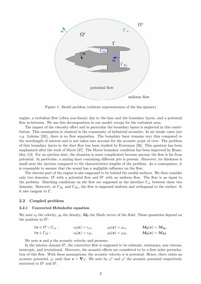
Figure 1: Model problem (without representation of the fan spinner)

engine, a turbulent flow (often non-linear) due to the fans and the boundary layers, and a potentialflow in-between. We use this decomposition in our model, except for the turbulent area.

The impact of the viscosity effect and in particular the boundary layers is neglected in this contri-bution. This assumption is classical in the community of industrial acoustics. In air intake cases (seee.g. Lidoine [33]), there is no flow separation. The boundary layer remains very thin compared tothe wavelength of interest and is not taken into account for the acoustic point of view. The problemof thin boundary layers in the duct flow has been studied by Eversman [26]. This question has beenemphasized after the work of Myers [37]. The Myers boundary condition has been improved by Bram-bley [12]. For an ejection duct, the situation is more complicated because anyway the flow is far frompotential. In particular, a mixing layer containing different jets is present. Moreover, its thickness issmall near the ejection compared to the characteristics lengths of the problem. As a consequence, itis reasonable to assume that the sound has a negligible influence on the flow.

The interior part of the engine is also supposed to be behind the modal surfaces. We then consideronly two domains: Ωi with a potential flow and Ωe with an uniform flow. The flow is an input tothe problem. Matching conditions on the flow are supposed at the interface Γ∞ between these twodomains. Moreover, at ΓM1 and ΓM2 , the flow is supposed uniform and orthogonal to the surface. Itit also tangent to Γ.

2.2 Coupled problem

2.2.1 Convected Helmholtz equation

We note c0 the celerity, ρ0 the density, M0 the Mach vector of the fluid. These quantities depend onthe position in Ωi:

∀x ∈ Ωe ∪ Γ∞ : c0(x) = c∞, ρ0(x) = ρ∞, M0(x) = M∞,

∀x ∈ ΓM : c0(x) = cM , ρ0(x) = ρM , M0(x) = MM .

We note v and p the acoustic velocity and pressure.In the interior domain Ωi, the convective flow is supposed to be subsonic, stationary, non viscous,

isentropic, and irrotational. Moreover, the acoustic effects are considered to be a first order perturba-tion of this flow. With these assumptions, the acoustic velocity v is potential. Hence, there exists anacoustic potential, ϕ, such that v = ∇ϕ. We note by ϕe and ϕi the acoustic potential respectivelyrestricted to Ωe and Ωi.

3

The physical quantities are associated with complex quantities with the following convention on,for instance, the acoustic potential: ϕ↔ < (ϕ exp(−iω0t)). The same notation is taken for the physicalquantity and its complex counterpart. In what follows, we always refer to the complex quantities. Thewavenumber depends on the position in Ωi:

k0(x) = k∞ :=ω0

c∞∀x ∈ Ωe ∪ Γ∞, k0(x) = kM :=

ω0

cM∀x ∈ ΓM .

For simplicity, only one modal surface ΓM is considered in the model problem instead of ΓM1 andΓM2 as presented on Figure 1. Following [42, p.259 eq.F27], and making use of the irrotationality ofthe carrier flow, the linearization of the Euler equations leads to

H(ϕ) = 0 in Ωi ∪ Γ∞ ∪ Ωe, (1)

where H(ϕ) := ρ0

(k2

0ϕ+ ik0M0 ·∇ϕ)

+ div [ρ0 (∇ϕ− (M0 ·∇ϕ)M0 + ik0ϕM0)]. This is the con-vected Helmholtz equation. We assume that Γ reflects perfectly the acoustic perturbations, yielding

∇ϕ · n = 0 on Γ. (2)

We now explain how the problem in Ωi is coupled to a problem in Ωe and a problem beyond ΓM bymeans of boundary conditions on Γ∞ and ΓM .

2.2.2 Coupling by means of boundary conditions

To focus on the coupling between the problem in Ωi and the one in Ωe, consider a test case like theone Figure 1, where some boundary condition is enforced on ΓM :

H(ϕ) = 0, in Ωi ∪ Γ∞ ∪ Ωe,

∇ϕ · n = 0, on Γ,

ϕ = g, on ΓM ,

Sommerfeld radiation condition,

(3)

where a Sommerfeld-like radiation condition is enforced to ensure uniqueness of problem by selectingoutgoing scattered waves and where g is some nonzero function defined on ΓM . Consider the followingproblem

H(ϕ) = 0, in Ωi,

H(ϕ) = 0, in Ωe,

[ϕ]Γ∞ = 0, on Γ∞,

[(∇ϕ− (M∞ ·∇ϕ)M∞ + ik∞ϕM∞) · n]Γ∞ = 0, on Γ∞,

∇ϕ · n = 0, on Γ,

ϕ = g, on ΓM ,

Sommerfeld-like radiation condition,

(4)

where [·]X denotes the jump of a quantity across a surface X.

Property 2.1. Problems 3 and 4 are equivalent.

Proof. If ϕ solves (3), it is clear that ϕ solves (4). Conversely, let ϕ defined in Ωi ∪ Ωe such that ϕverifies (4). From [34, Lemma 4.19], since ϕ verifies lines 1, 2, 3, 4 of (4), then ϕ verifies line 1 of (3),which finishes the proof.

Using the transmission conditions of problem (4) on Γ∞, we will write problem (3) in the form ofa problem on ϕi and a boundary condition on Γ∞. Consider the following problem in Ωe

H(ϕe) = 0, in Ωe,

ϕe = F, on Γ∞,

Sommerfeld-like radiation condition,

(5)

4

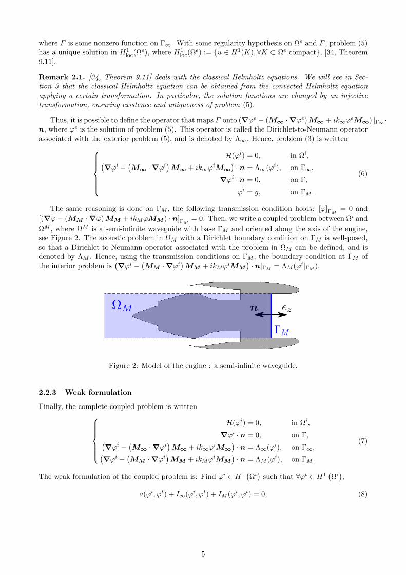
where F is some nonzero function on Γ∞. With some regularity hypothesis on Ωe and F , problem (5)has a unique solution in H1

loc(Ωe), where H1

loc(Ωe) := u ∈ H1(K), ∀K ⊂ Ωe compact, [34, Theorem

9.11].

Remark 2.1. [34, Theorem 9.11] deals with the classical Helmholtz equations. We will see in Sec-tion 3 that the classical Helmholtz equation can be obtained from the convected Helmholtz equationapplying a certain transformation. In particular, the solution functions are changed by an injectivetransformation, ensuring existence and uniqueness of problem (5).

Thus, it is possible to define the operator that maps F onto (∇ϕe − (M∞ ·∇ϕe)M∞ + ik∞ϕeM∞) |Γ∞ ·

n, where ϕe is the solution of problem (5). This operator is called the Dirichlet-to-Neumann operatorassociated with the exterior problem (5), and is denoted by Λ∞. Hence, problem (3) is written

H(ϕi) = 0, in Ωi,(∇ϕi −

(M∞ ·∇ϕi

)M∞ + ik∞ϕ

iM∞)· n = Λ∞(ϕi), on Γ∞,

∇ϕi · n = 0, on Γ,

ϕi = g, on ΓM .

(6)

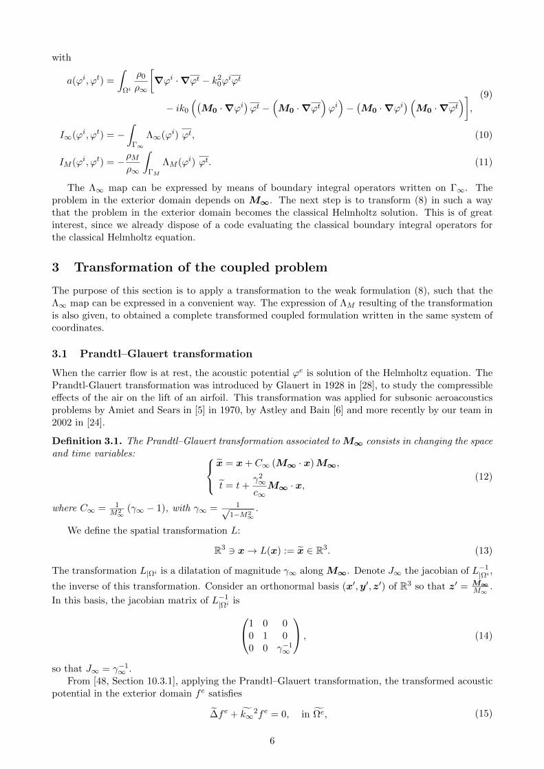
The same reasoning is done on ΓM , the following transmission condition holds: [ϕ]ΓM= 0 and

[(∇ϕ− (MM ·∇ϕ)MM + ikMϕMM ) · n]ΓM= 0. Then, we write a coupled problem between Ωi and

ΩM , where ΩM is a semi-infinite waveguide with base ΓM and oriented along the axis of the engine,see Figure 2. The acoustic problem in ΩM with a Dirichlet boundary condition on ΓM is well-posed,so that a Dirichlet-to-Neumann operator associated with the problem in ΩM can be defined, and isdenoted by ΛM . Hence, using the transmission conditions on ΓM , the boundary condition at ΓM ofthe interior problem is

(∇ϕi −

(MM ·∇ϕi

)MM + ikMϕ

iMM

)· n|ΓM

= ΛM (ϕi|ΓM).

Figure 2: Model of the engine : a semi-infinite waveguide.

2.2.3 Weak formulation

Finally, the complete coupled problem is writtenH(ϕi) = 0, in Ωi,

∇ϕi · n = 0, on Γ,(∇ϕi −

(M∞ ·∇ϕi

)M∞ + ik∞ϕ

iM∞)· n = Λ∞(ϕi), on Γ∞,(

∇ϕi −(MM ·∇ϕi

)MM + ikMϕ

iMM

)· n = ΛM (ϕi), on ΓM .

(7)

The weak formulation of the coupled problem is: Find ϕi ∈ H1(Ωi)

such that ∀ϕt ∈ H1(Ωi),

a(ϕi, ϕt) + I∞(ϕi, ϕt) + IM (ϕi, ϕt) = 0, (8)

5

with

a(ϕi, ϕt) =

∫Ωi

ρ0

ρ∞

[∇ϕi ·∇ϕt − k2

0ϕiϕt

− ik0

((M0 ·∇ϕi

)ϕt −

(M0 ·∇ϕt

)ϕi)−(M0 ·∇ϕi

) (M0 ·∇ϕt

)],

(9)

I∞(ϕi, ϕt) = −∫

Γ∞

Λ∞(ϕi) ϕt, (10)

IM (ϕi, ϕt) = −ρMρ∞

∫ΓM

ΛM (ϕi) ϕt. (11)

The Λ∞ map can be expressed by means of boundary integral operators written on Γ∞. Theproblem in the exterior domain depends on M∞. The next step is to transform (8) in such a waythat the problem in the exterior domain becomes the classical Helmholtz solution. This is of greatinterest, since we already dispose of a code evaluating the classical boundary integral operators forthe classical Helmholtz equation.

3 Transformation of the coupled problem

The purpose of this section is to apply a transformation to the weak formulation (8), such that theΛ∞ map can be expressed in a convenient way. The expression of ΛM resulting of the transformationis also given, to obtained a complete transformed coupled formulation written in the same system ofcoordinates.

3.1 Prandtl–Glauert transformation

When the carrier flow is at rest, the acoustic potential ϕe is solution of the Helmholtz equation. ThePrandtl-Glauert transformation was introduced by Glauert in 1928 in [28], to study the compressibleeffects of the air on the lift of an airfoil. This transformation was applied for subsonic aeroacousticsproblems by Amiet and Sears in [5] in 1970, by Astley and Bain [6] and more recently by our team in2002 in [24].

Definition 3.1. The Prandtl–Glauert transformation associated to M∞ consists in changing the spaceand time variables:

x = x + C∞ (M∞ · x)M∞,

t = t+γ2∞c∞

M∞ · x,(12)

where C∞ = 1M2∞

(γ∞ − 1), with γ∞ = 1√1−M2

∞.

We define the spatial transformation L:

R3 3 x→ L(x) := x ∈ R3. (13)

The transformation L|Ωi is a dilatation of magnitude γ∞ along M∞. Denote J∞ the jacobian of L−1|Ωi ,

the inverse of this transformation. Consider an orthonormal basis (x′,y′, z′) of R3 so that z′ = M∞M∞

.

In this basis, the jacobian matrix of L−1|Ωi is1 0 0

0 1 00 0 γ−1

∞

, (14)

so that J∞ = γ−1∞ .

From [48, Section 10.3.1], applying the Prandtl–Glauert transformation, the transformed acousticpotential in the exterior domain fe satisfies

∆fe + k∞2fe = 0, in Ωe, (15)

6

where k∞ := γ∞k∞ is the modified wavenumber. This is a classical Helmholtz equation. The Som-merfeld radiation condition

r

(∂fe

∂r− ik∞fe

)→ 0, r → +∞ (16)

is enforced as well to ensure uniqueness of the solution [44].

Remark 3.1 (Coordinate transformations). Other coordinate transformation can retrieve the classi-cal Helmholtz equation from the uniformly convected Helmholtz equation. For instance, Lorentz-liketransformation are possible, but would lead to frequency dependent meshes, which is not desirable. Thecoordinate transformation (12) we used belongs to a general family of transformations proposed in [17].With (12), the flux of the Poynting vector is conserved through any surface orthogonal to M∞.

Remark 3.2. We define a Prandtl–Glauert transformation associated to another vectors v by changingM∞ and M∞ by respectively v and ‖v‖ in Definition 3.1. In what follows, we note by · the objects andoperators transformed by the Prandtl–Glauert transformation associated to M∞ (normals, geometry,derivatives).

3.2 Transformation of the volume integral term a (9)

In what follows, the Prandlt-Glauert transformation is carried-out in the interior domain after theweak formulation has been written. Doing so, the obtained formulation is written in a form that usesoperators that are already implemented in the code ACTIPOLE [21, 22]. Another choice can be tocarry out the Prandlt-Glauert transformation first, and then write the weak formulation. The twoformulations are equivalent, but this last case suits well the study of the existence and uniqueness ofthe formulation (see [16]).

Consider the solution function φi(t,x) = ϕi(x)e−iωt. Applying the Prandtl–Glauert transforma-

tion (12), this function transforms into ϕi(L−1(x))eik∞γ2∞M∞·L−1(x)e−iωt. This motivates the intro-

duction of the function f i, such that f i(x) = ϕi(x)E∞(x), where E∞(x) = eik∞γ2∞M∞·x. We define f t

from the test function ϕt in the same fashion. This leads to

ϕi(x) = f i(x)E∞(x)

ϕt(x) = f t(x)E∞(x).(17)

The transformation H1(Ωi) 3 ϕt(x)→ f t(x)E∞(x) ∈ H1(Ωi) is surjective, and therefore this modifi-cation of test function is still compatible with the weak formulation. The gradients are transformedto

∇ϕi(x) =(∇f i(x)− ik∞γ2

∞M∞fi(x)

)E∞(x)

∇ϕt(x) =(∇f t(x) + ik∞γ

2∞M∞f t(x)

)E∞(x).

(18)

Thus, Equation (9) becomes

a(ϕi, ϕt) =

∫Ωi

ρ0

ρ∞

[(L−f i

)·(L+f t

)− k2

0fif t − ik0

((M0 ·

(L−f i

))f t

−(M0 ·

(L+f t

))f i)]−∫

Ωi

ρ0

ρ∞

(M0 ·

(L−f i

)) (M0 ·

(L+f t

)),

(19)

where L± := ∇± ik∞γ2∞M∞ and where we used E∞(x)E∞(x) = 1.

Then, applying the change of variables and making use of the jacobian J∞ of L−1|Ωi , there holds

a(ϕi, ϕt) = J∞

∫Ωi

ρ0

ρ∞

[(L−f i

)·(L+f t

)− k2

0fif t − ik0

((M0 ·

(L−f i

))f t

−(M0 ·

(L+f t

))f i)]− J∞

∫Ωi

ρ0

ρ∞

(M0 ·

(L−f i

))(M0 ·

(L+f t

)),

(20)

7

where L± := ∇ +(C∞M∞ · ∇± ik∞γ2

∞

)M∞. Notice that when changing the variables, we wrote

the differential operators in the transformed system of coordination, using

∇→ ∇ + C∞M∞M∞ · ∇, (21)

which is directly derived from the first line of (12).

Remark 3.3. If we impose M0 = M∞, ρ0 = ρ∞ and c0 = c∞ in (20), we find

a(ϕi, ϕt) = J∞

∫Ωi

(∇f i · ∇f t − k∞2f if t

), (22)

which is the variational formulation for the nonconvected Helmholtz equation with modified wavenumberk∞ = γ∞k∞ on f on the transformed geometry and in the transformed coordinates.

Remark 3.4. The expression (20) for the volume integral is more complicated than the expression (9).However, this will enable us to treat the coupling with the exterior domain in a simple way.

3.3 Transformation of the surface integral term I∞ (10)

3.3.1 Transformation of normals

Consider a closed surface C defined by a function Φ by Φ(x) = 0, and denote by C the transformationof C by L. Let x ∈ C, the normal to C at x, n(x), is colinear to ∇Φ(x), whereas the normal to C atx, n(x), is colinear to ∇Φ(x). From (21), there then holds

n(x) = K∞(x) (n (x) + C∞ (M∞ · n (x))M∞) , (23)

where K∞(x) is a normalization factor. Taking the square of the norm of both sides of (23), there

holds 1 = K∞(x)2(

1 + (M2∞C

2∞ + 2C∞) (M∞ · n (x))2

), from which we deduce

K∞(x) =

√1 + (γ∞M∞ · n (x))2. (24)

Conversely, to express n (x) as a function of n(x), we consider the inverse spatial transformationL−1, which consists of a contraction of magnitude γ−1

∞ along M∞. The gradient are then changed as

∇→ ∇ + C∞M∞M∞ ·∇, where C∞ = 1M2∞

(γ−1∞ − 1

). Applying this to the gradient of Φ(x) = 0,

which defines C, we deduce

n(x) = K∞(x)(n (x) + C∞ (M∞ · n (x))M∞

), (25)

where K∞(x) is a normalization factor. Using the normalization condition,

K∞(x) =1√

1− (M∞ · n (x))2. (26)

3.3.2 Jacobian of the spatial transformation restricted to Γ∞

Consider L|Γ∞ , the restriction of L to the 2-dimensional manifold Γ∞. Let x ∈ Γ∞. Let m1 := M∞M∞

,

m2 := n−(m1·n)m1

‖n−(m1·n)m1‖ and m3 such that (m1,m2,m3) is an orthonormal triplet. Let N := n ·m1. By

construction, n = Nm1 +√

1−N2m2. Then, we define t1 := −√

1−N2m1 +Nm2 and t2 := m3,see Figure 3. It is direct to verify that (t1, t2) is an orthonormal doublet, and that t1 ·n = t2 ·n = 0.Therefore, (t1, t2) is an orthonormal basis for the hyperplane tangent to Γ∞ in x, and |Jac(L|Γ∞)| =|det (L(t1), L(t2)) |. Since we have identified in t1 and t2 the components parallel and orthogonal toM∞, there holds L(t1) = −γ∞

√1−N2m1 + Nm2 and L(t2) = t2 = m3, because t2 is orthogonal

to M∞. We see that L(t1) and L(t2) are orthogonal, then det (L(t1), L(t2)) = ‖L(t1)‖‖L(t2)‖ =

‖L(t1)‖ =√N2 + γ2

∞(1−N2) = γ∞√

1− (M∞ · n)2, from which we deduce |Jac(L−1|Γ∞)| = J∞K∞.

8

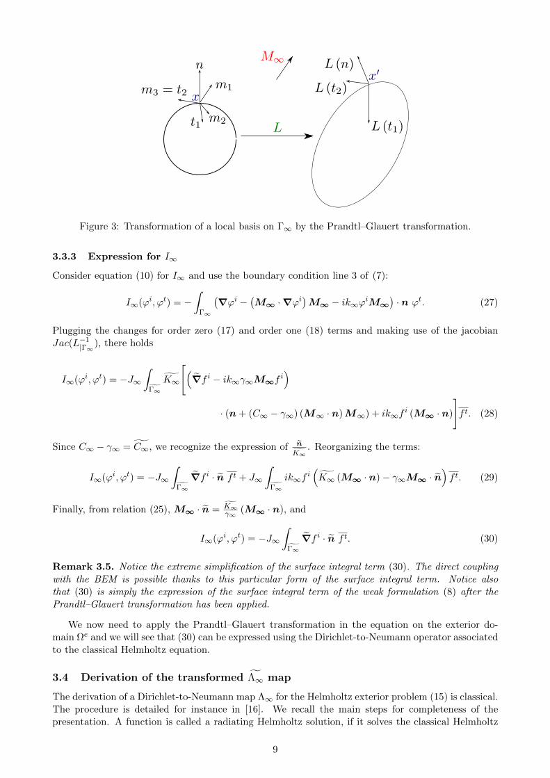
Figure 3: Transformation of a local basis on Γ∞ by the Prandtl–Glauert transformation.

3.3.3 Expression for I∞

Consider equation (10) for I∞ and use the boundary condition line 3 of (7):

I∞(ϕi, ϕt) = −∫

Γ∞

(∇ϕi −

(M∞ ·∇ϕi

)M∞ − ik∞ϕiM∞

)· n ϕt. (27)

Plugging the changes for order zero (17) and order one (18) terms and making use of the jacobianJac(L−1

|Γ∞), there holds

I∞(ϕi, ϕt) = −J∞∫

Γ∞

K∞

[(∇f i − ik∞γ∞M∞f

i)

· (n + (C∞ − γ∞) (M∞ · n)M∞) + ik∞fi (M∞ · n)

]f t. (28)

Since C∞ − γ∞ = C∞, we recognize the expression of n

K∞. Reorganizing the terms:

I∞(ϕi, ϕt) = −J∞∫

Γ∞

∇f i · n f t + J∞

∫Γ∞

ik∞fi(K∞ (M∞ · n)− γ∞M∞ · n

)f t. (29)

Finally, from relation (25), M∞ · n = K∞γ∞

(M∞ · n), and

I∞(ϕi, ϕt) = −J∞∫

Γ∞

∇f i · n f t. (30)

Remark 3.5. Notice the extreme simplification of the surface integral term (30). The direct couplingwith the BEM is possible thanks to this particular form of the surface integral term. Notice alsothat (30) is simply the expression of the surface integral term of the weak formulation (8) after thePrandtl–Glauert transformation has been applied.

We now need to apply the Prandtl–Glauert transformation in the equation on the exterior do-main Ωe and we will see that (30) can be expressed using the Dirichlet-to-Neumann operator associatedto the classical Helmholtz equation.

3.4 Derivation of the transformed Λ∞ map

The derivation of a Dirichlet-to-Neumann map Λ∞ for the Helmholtz exterior problem (15) is classical.The procedure is detailed for instance in [16]. We recall the main steps for completeness of thepresentation. A function is called a radiating Helmholtz solution, if it solves the classical Helmholtz

9

solution in Ωe and in R3\Ωe, and if it satisfies the Sommerfeld radiation condition. A radiatingHelmholtz solution v can be represented from the jump of its traces on Γ [38, Theorem 3.1.1]

v = −S [∇v · n] +D [v] in Ωe ∪ R3\Ωe, (31)

where S and D are the single-layer and double-layer potentials associated with the Helmholtz equation,defined such that

Sλ(x) =

∫Γ∞

G(x,y)λ(y) dy, Dµ(x) =

∫Γ∞

∂G(x,y)

∂nxλ(y) dy, ∀x ∈ Ωe ∪ R3\Ωe,

where G(x,y) := exp(−ik∞|x−y|)4π|x−y| is the fundamental solution to the classical Helmholtz equation with

wavenumber k∞. If v is a radiating Helmholtz solution, then [38, Theorem 3.1.2][12I −D SN 1

2I +D∗

] [[v]Γ∞

[∇v · n]Γ∞

]= −

[vi

∇vi · n

]on Γ∞, (32)

where S, D, D∗ and N are respectively the single-layer, double-layer, transpose of the double-layerand hypersingular boundary integral operators defined as, ∀x ∈ Γ∞,

Sλ(x) =

∫Γ∞

G(x,y)λ(y)dy, Dµ(x) =

∫Γ∞

∂G(x,y)

∂nyµ(y)dy,

D∗λ(x) =

∫Γ∞

∂G(x,y)

∂nxλ(y)dy, Nµ(x) =

∮Γ∞

∂2G(x,y)

∂nx∂nyµ(y)dy.

Consider the function u such that u|Ωe := fe and u|

Ωi := 0, where fe solves (15), so that u is aradiating Helmholtz solution in the transformed coordinates and on the transformed geometry.

Remark 3.6. We chose u|Ωi := 0 to ensure that u|

Ωi solves the Helmholtz equation in Ωi, which isclearly the case, and to ensure that u is a radiating Helmholtz solution, to apply (32). We could havechosen any solution to the Helmholtz equation in Ωi for u|

Ωi, but in this case, the relation (32) wouldhave involve jumps of traces of some function not related to the problem. Our choice is motivated bythe fact that, with u|

Ωe := fe and u|Ωi := 0, [u]

Γ∞= fe|

Γ∞and [∇u · n]

Γ∞= ∇fe · n|

Γ∞, so that the

relation (32) only involves the total transformed acoustic potential on Γ∞, which will provide a simplecoupling with (30).

Consider the transmission conditions (4), lines 3 and 4. Applying the Prandtl–Glauert transfor-mation (using the first line of (17) and (18)) and making use of (23), there holds [f ]

Γ∞= 0,[

∇f · n]

Γ∞= 0,

(33)

which we can writef i = fe = f, on Γ∞,

∇f i · n = ∇fe · n = ∇f · n, on Γ∞.(34)

Using (32) with v = u yields[12I − D S

N 12I + D∗

] [f

∇f · n

]=

[00

], on Γ∞, (35)

where S, D, D∗ and N are respectively the single-layer, double-layer, transpose of the double-layer andhypersingular boundary integral operators for the Helmholtz equation obtained in the Prandtl–Glauerttransformed space with modified wavenumber k∞:

Sλ(x) =

∫Γ∞

G(x, y)λ(y)dy, Dµ(x) =

∫Γ∞

∂G(x, y)

∂nyµ(y)dy,

D∗λ(x) =

∫Γ∞

∂G(x, y)

∂nxλ(y)dy, Nµ(x) =

∮Γ∞

∂2G(x, y)

∂nx∂nyµ(y)dy,

10

where G(x,y) :=exp(−ik∞|x−y|

)4π|x−y| is the fundamental solution to the classical Helmholtz equation with

modified wavenumber k∞.Using the first line of (35), there holds

∇f · n = S−1

(D − 1

2I

)(f). (36)

Then, we subtract ∇f · n from the second line of (35) and inverse the signs to obtain

∇f · n = −N(f) +

(1

2I − D∗

)(∇f · n

). (37)

Injecting (36) into the right-hand side of (37), an expression of the Λ∞ map can be obtained in thefollowing form:

∇f · n = Λ∞ (f) := −N(f) +

(1

2I − D∗

)S−1

(D − 1

2I

)(f). (38)

Notice that other Λ∞ maps can be readily obtained from (35). Our choice leads to a symmetric linearsystem (see the matrix (54)), for which computation optimizations can be used.

Remark 3.7. Even though it is possible to write integral equations for the uniformly convectedHelmholtz equation (see [7]), the Prandtl–Glauert transformation allows us to write integral equa-tion that only involves the Green kernel associated to the Helmholtz equation. Hence, we can profitfrom our validated code ACTIPOLE developed by our team [21, 22].

3.5 Computation of the coupling integral term IM (11)

The engine is modeled by a semi-infinite waveguide with the classical hypothesis that the flow isuniform. To simplify the presentation, the waveguide is also supposed to be oriented along the localaxis ez so that ΓM is orthogonal to ez (see Figure 2). More precisely, we suppose here that ΓM isincluded in the plane z = 0. The flow is defined by MM and is then parallel to ez. A more generalformulation is presented in appendix A.1.

In ΩM , the acoustic potential is decomposed into an incident and a diffracted potential: ϕ :=ϕinc + ϕdiff , both solution to the following convected Helmholtz equation:

∆ϕinc,diff + k2Mϕ

inc,diff + 2ikMMM ·∇ϕinc,diff −MM ·∇(MM ·∇ϕinc,diff

)= 0 in ΩM . (39)

The incident potential is known, whereas the diffracted potential is unknown. Under these assump-tions, the following decomposition holds [36, 13]:

ϕinc(x, y, z) =∑(ι)

αι vι(x, y) exp(ik+ι z)

in ΩM ,

ϕdiff(x, y, z) =∑(ι)

βι vι(x, y) exp(ik−ι z

)in ΩM ,

(40)

with ι a discrete index and where the incident modal coefficients αι :=∫

ΓMϕincvι are supposed known

(input of the problem) while the diffracted modal coefficients βι :=∫

ΓMϕdiffvι are some unknowns of

the problem. The basis functions vι constitute a modal basis function chosen to be orthonormal.For instance for a cylindrical duct of radius R, ι corresponds to a couple of indices (m,n) ∈ (Z×N∗)

and the functions vι are defined in polar coordinates by [36, 13]

vι(r, θ) = vm,n(r, θ) := Vm,n Jm

(rm,nR

r)

exp (imθ) , (41)

11

with rm,n the n-th zero of the derivative of m-th Bessel function of the first kind Jm, Vm,n thenormalization factor such that

∫ΓM

v2m,n = 1, and

k±ι = k±mn =−kMMM ±

√k2M −

(1−M2

M

) (rm,nR

)2

1−M2M

for propagating modes (k±mn ∈ R), (42)

k±ι = k±mn =−kMMM ± i

√(1−M2

M

) (rm,nR

)2− k2

M

1−M2M

for evanescent modes (k±mn ∈ C), (43)

the wavenumber of each mode. For any (m,n) ∈ (Z×N∗), the corresponding mode is either propagatingor evanescent. For any shape of the duct, there exist a finite number of propagating modes and aninfinite number of evanescent modes.

Based on this decomposition, the expression of the Dirichlet-to-Neumann operator ΛM is [10, 31]:

(∇ϕ− (MM ·∇ϕ)MM + ikMϕMM ) · n = ΛM (ϕ) :=∑(ι)

(αιY

+ι + βιY

−ι

)vι on ΓM , (44)

where

Y ±ι := −i[k±ι(1−M2

M

)+ kMMM

](45)

By definition,

IM (ϕ,ϕt) = −ρMρ∞

∫ΓM

ΛM (ϕ) ϕt

= −ρMρ∞

∑(ι)

αιY+ι

∫ΓM

vι ϕt −ρMρ∞

∑(ι)

βιY−ι

∫ΓM

vι ϕt.

Notice that since ΓM is included in the plane z = 0 and M∞ is directed along ez, then ΓM = ΓM ,and vι = vι on ΓM , where vι is the Prandtl–Glauert transformation of vι. Hence, αι =

∫ΓM

f incvι and

βι =∫

ΓMfdiffvι, where f inc and fdiff are the Prandtl–Glauert transformation of respectively ϕinc and

ϕdiff. In view of the coupling in the coordinates and geometry transformed by the Prandtl–Glauerttransformation, we can write

IM (ϕ,ϕt) = −ρMρ∞

∑(ι)

(αιY

+ι + βιY

−ι

) ∫ΓM

vιf t (46)

with f t the Prandtl–Glauert transformation of ϕt. Let us define γκ by f t =∑(κ)

γκvκ. Then, using the

orthonormality of the modal basis∫

ΓMvιvκ = δι,κ, where δι,κ refers to the Kronecker delta, we obtain

IM (ϕ,ϕt) = −ρMρ∞

∑(ι)

(αιY

+ι + βιY

−ι

)γι. (47)

To write a direct coupled problem, it is more practical to consider the coefficient of decomposition ofthe total acoustic potential. Consider ςι :=

∫ΓM

ϕvι = αι + βι, there holds

IM (ϕ,ϕt) = −ρMρ∞

∑(ι)

(αι(Y +ι − Y −ι

)+ ςιY

−ι

)γι. (48)

12

3.6 Transformed coupled problem

To treat the operator inversion in the definition (38) of Λ∞, we introduce λ ∈ H−12 (Γ∞) such that

λ :=(S)−1((

D − 1

2I

)f

), (49)

so that Λ∞ (f) = −Nf +

(1

2I − D∗

)λ,(

D − 1

2I

)f − Sλ = 0.

(50)

Plugging (50) into (30) and using the expression (48) in (8) leads to the following weak formulation

for the coupled problem: find (f, λ) ∈ H1(Ωi)×H−12 (Γ∞) such that ∀

(f t, λt,

)∈ H1(Ωi)×H−

12 (Γ∞),

a(f, f t) + J∞

∫Γ∞

Nf f t + J∞

∫Γ∞

(D∗ − 1

2I

)λ f t − ρM

ρ∞

∑(ι)

ςιY−ι γι

=ρMρ∞

∑(ι)

αι(Y +ι − Y −ι

)γι,

J∞

∫Γ∞

(D − 1

2I

)f λt − J∞

∫Γ∞

Sλ λt = 0.

(51)

with ςι and γι such that∑(ι)

|ςι|2∣∣Y ±ι ∣∣ <∞ and

∑(ι)

|γι|2∣∣Y ±ι ∣∣ <∞ and with a(f, f t) = a(ϕ,ϕt), where

a is defined in (20).

4 Methodologies for the numerical resolutions

The weak formulation (51) has to be solved numerically. To do so, we first introduce an unstructured

volumic mesh Vh of the domain Ωi made of tetrahedrons. The surfacic meshes Sh,M and Sh,∞ are

obtained as the boundary faces of Vh associated to ΓM and Γ∞ respectively. We denote V1h and S1

h,M

the finite element spaces P1 on respectively Vh and Sh,M , and S0h,∞ the finite element space P0 on

Sh,∞. To introduce a numerical approximation, we have to consider a finite number of modes. Weconsider then M inc

tot incident modes and M′difftot diffracted modes, with M

′difftot ≥M inc

tot .We obtain the following discrete conforming approximation of (51): Find (fh, λh) ∈ V1

h × S0h,∞

such that ∀(f th, λ

th,)∈ V1

h × S0h,∞,

a(fh, fth) + J∞

∫Γ∞

Nfh fht + J∞

∫Γ∞

(D∗ − 1

2I

)λh fh

t − ρMρ∞

M′difftot∑(ι)

ςιY−ι γι

=ρMρ∞

M′difftot∑(ι)

αι(Y +ι − Y −ι

)γι,

J∞

∫Γ∞

(D − 1

2I

)fhλ

th − J∞

∫Γ∞

Sλh λth = 0,

(52)

with ςι and γι such that∑(ι)

|ςι|2∣∣Y ±ι ∣∣ < ∞ and

∑(ι)

|γι|2∣∣Y ±ι ∣∣ < ∞. Notice that since M

′difftot ≥ M inc

tot ,

then some αι are zero.Let (θi)1≤i≤p and (ψi)1≤i≤q denote finite element bases for V1

h and S0h,∞ respectively. The de-

composition of fh ∈ V1h and λh ∈ S0

h,∞ on these bases are written in the form fh =∑p

i=1 fiθi and

13

λh =∑q

i=1 λiψi. Let

u :=

((fi) 1≤i≤p(λi) 1≤i≤q

), b :=

ρMρ∞

M′difftot∑(ι)

αι(Y +ι − Y −ι

) ∫ΓM

vι θi

1≤i≤p

(0) 1≤i≤q

, (53)

and

A :=

Cij J∞

∫Γ∞

(D∗ − 1

2I

)ψj θi

J∞

∫Γ∞

(D − 1

2I

)θj ψi −J∞

∫Γ∞

Sψj ψi

, (54)

with

Cij := a(θj , θi) + J∞

∫Γ∞

Nθj θi −ρMρ∞

M′difftot∑(ι)

Y −ι

∫ΓM

vι θi

∫ΓM

θj vι. (55)

The linear system resulting from (51) isAu = b. (56)

The matrix A contains both dense and sparse blocks. By reordering the unknowns in order to

separate the unknowns related to Ωi and to Γ∞ (indexed respectively by V and Γ in the following),the linear system can be written (

AV V AV Γ

AΓV AΓΓ

)(uVuΓ

)=

(bVbΓ

)(57)

with AV V , AV Γ and AΓV being sparse matrices and AΓΓ a dense matrix.To solve (57), a block Gaussian elimination, known as the Schur complement [49], is first carried

out on the sparse matrices to eliminate the unknowns of the volume domain. The remaining systemis then (

AΓΓ −AΓVA−1V VAV Γ

)uΓ = bΓ −AΓVA

−1V V bV (58)

This linear system can then be solved either with a direct classical LU solver or an iterative solver.Moreover in the case of the iterative solver, the fast multipole method (FMM) [41, 45, 27] can beused to take into account the dense matrix AΓΓ relative to the BEM formulation. The conditioningof the remaining system is driven by the BEM matrix. The classical SPAI preconditioner for BEMformulation [15] of matrix AΓΓ is then used to improve the converge of the iterative solver for equation(58).

These resolution strategies are implemented in the ACTIPOLE software and make use of theMUMPS solver [3, 4] for the sparse matrix elimination and of an in-house solver with out-core andMPI functionalities for the remaining system.

5 Numerical results

Even if the test cases are axisymmetric, all the following computations are full-3D computations. Theyhave been run on a machine with 2x6 intel Xeon “Westmere” processors running at 3.06GHz with72GB RAM per node and infiniband QDR.

5.1 Zero flow

The first test case is designed to check the validity of the modeling for a non-uniform medium withoutflow and of the FEM-BEM coupling. It consists of a sphere of radius 1 m centered at the originwith different fluid properties: ρ0 = ρ∞, c0 = 2c∞ inside the sphere and ρ∞ = 1.2 kg.m−3, c∞ =340 m.s−1 outside the sphere. The acoustic potential source is a monopole located outside the sphere

14

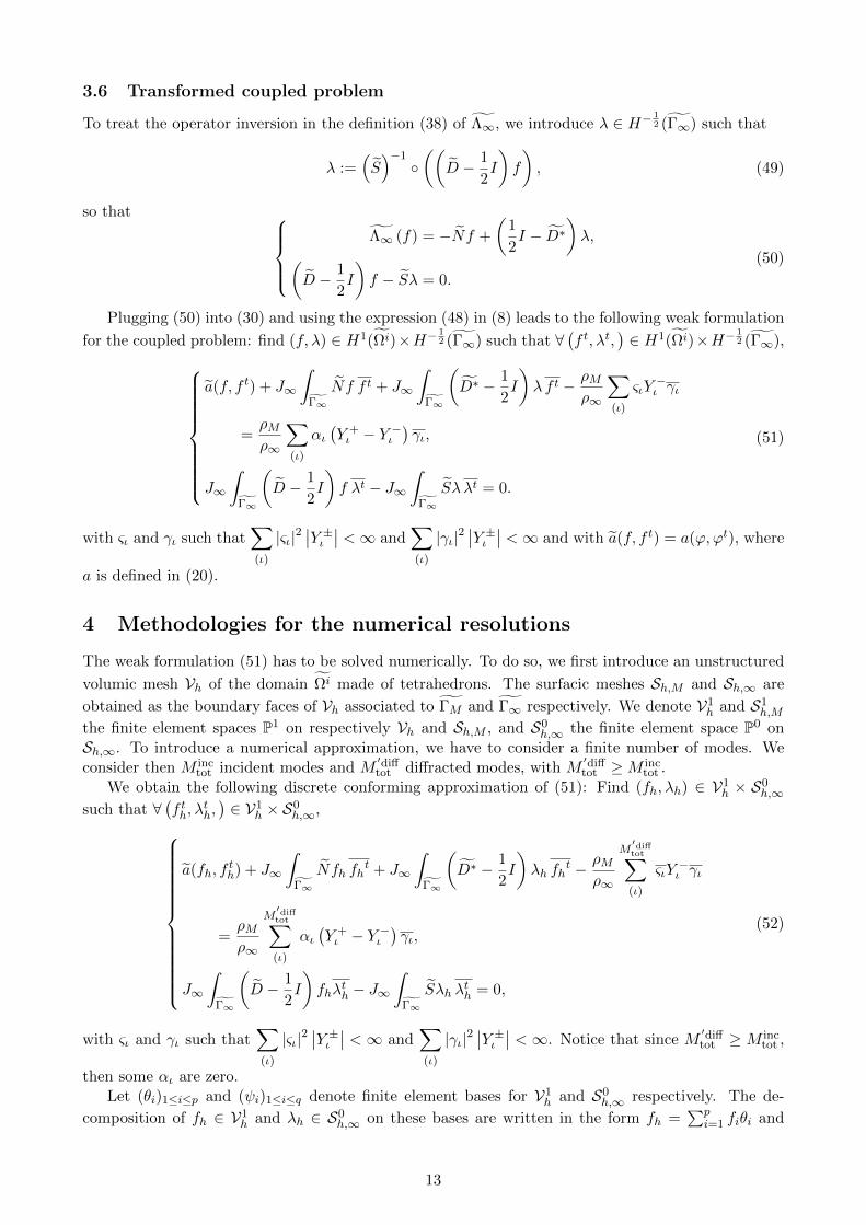
at (0., 0., 2.5). The observable is located outside the sphere at (0, 1.7, 0) and the frequency range ofinterest is 11 to 500 Hz.

The reference result is obtained by a Mie series and the comparison of the scattered pressurewith the FEM-BEM solution is visible on Figure 4. The volumic domain used for the FEM-BEMcomputation is a sphere of radius 1.07 m to ensure the continuity of the speed of sound at Γ∞. Themesh has an average edge length of 85 mm (λ/8 for 500 Hz, the highest frequency) and contains 19,494dofs (80,616 tetrahedrons and 4,672 triangles on Γ∞). The relative error on the module of the totalpressure is between 7× 10−4 (at 100 Hz) and 3× 10−2 (at 500 Hz).

Figure 4: Zero flow: Real part of the scattered pressure at the sensor in function of the frequency(validation of the FEM-BEM on the sphere test case).

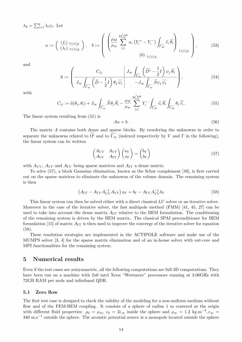
5.2 Modal test case without flow

Consider a modal cylindrical duct of length L = 1 m and radius R = 0.25 m without flow (Figure5). The frequency of the source is 2,040 Hz. Three kinds of computation have been performed withACTIPOLE: classical BEM formulation, full FEM formulation, coupled FEM-BEM formulation in thesame domain of computation. The iterative solver has been chosen with a tolerance on the residualof 10−8. Comparisons have been carried out on the transmission coefficients between ΓM1 and ΓM2 of

Figure 5: Geometry of the modal test case.

the mode m = 0, n = 1 (Table 1) and their theoretical values.

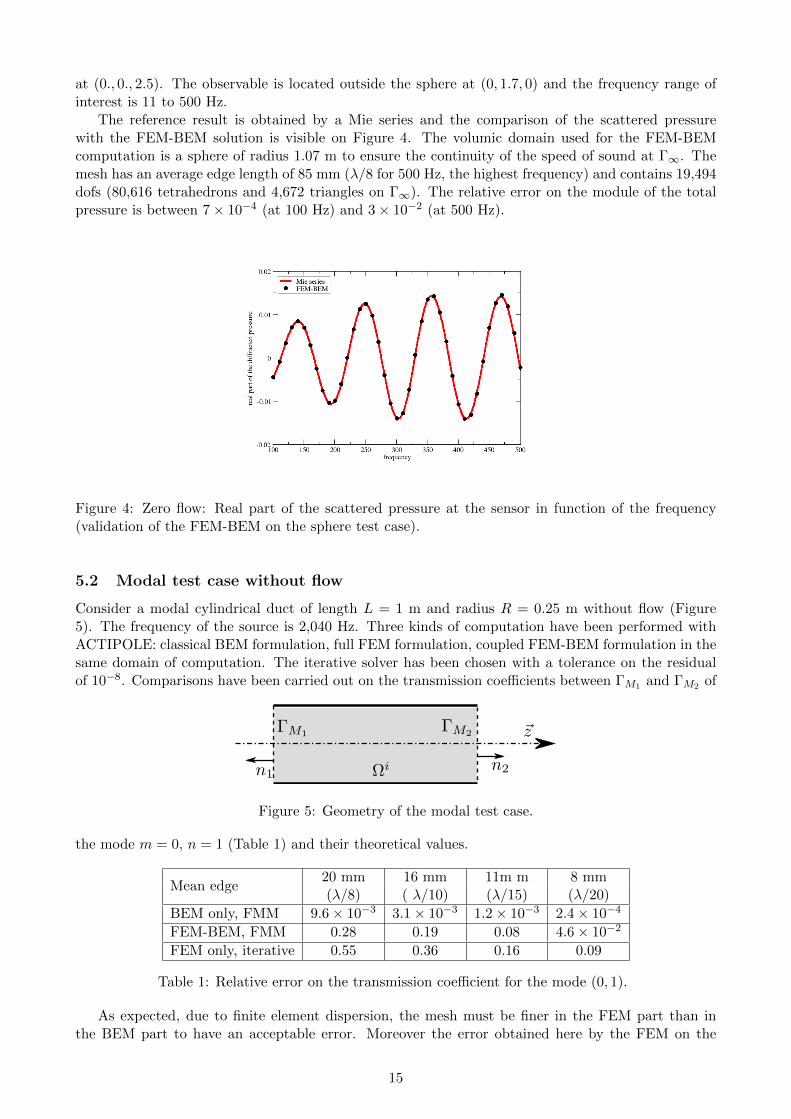
Mean edge20 mm 16 mm 11m m 8 mm(λ/8) ( λ/10) (λ/15) (λ/20)

BEM only, FMM 9.6× 10−3 3.1× 10−3 1.2× 10−3 2.4× 10−4

FEM-BEM, FMM 0.28 0.19 0.08 4.6× 10−2

FEM only, iterative 0.55 0.36 0.16 0.09

Table 1: Relative error on the transmission coefficient for the mode (0, 1).

As expected, due to finite element dispersion, the mesh must be finer in the FEM part than inthe BEM part to have an acceptable error. Moreover the error obtained here by the FEM on the

15

transmission coefficient has a linear dependency on the length of the FEM domain and a squaredependency on the size of the elements.

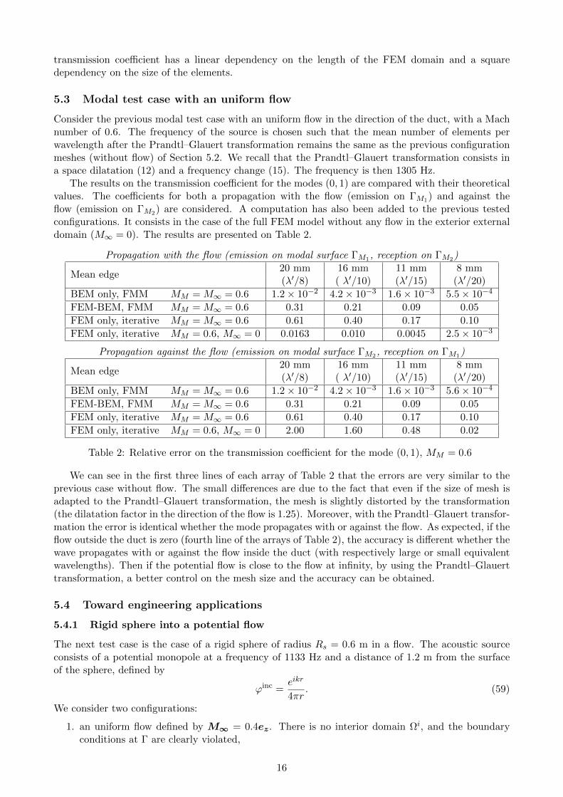
5.3 Modal test case with an uniform flow

Consider the previous modal test case with an uniform flow in the direction of the duct, with a Machnumber of 0.6. The frequency of the source is chosen such that the mean number of elements perwavelength after the Prandtl–Glauert transformation remains the same as the previous configurationmeshes (without flow) of Section 5.2. We recall that the Prandtl–Glauert transformation consists ina space dilatation (12) and a frequency change (15). The frequency is then 1305 Hz.

The results on the transmission coefficient for the modes (0, 1) are compared with their theoreticalvalues. The coefficients for both a propagation with the flow (emission on ΓM1) and against theflow (emission on ΓM2) are considered. A computation has also been added to the previous testedconfigurations. It consists in the case of the full FEM model without any flow in the exterior externaldomain (M∞ = 0). The results are presented on Table 2.

Propagation with the flow (emission on modal surface ΓM1, reception on ΓM2)

Mean edge20 mm 16 mm 11 mm 8 mm(λ′/8) ( λ′/10) (λ′/15) (λ′/20)

BEM only, FMM MM = M∞ = 0.6 1.2× 10−2 4.2× 10−3 1.6× 10−3 5.5× 10−4

FEM-BEM, FMM MM = M∞ = 0.6 0.31 0.21 0.09 0.05

FEM only, iterative MM = M∞ = 0.6 0.61 0.40 0.17 0.10

FEM only, iterative MM = 0.6, M∞ = 0 0.0163 0.010 0.0045 2.5× 10−3

Propagation against the flow (emission on modal surface ΓM2, reception on ΓM1)

Mean edge20 mm 16 mm 11 mm 8 mm(λ′/8) ( λ′/10) (λ′/15) (λ′/20)

BEM only, FMM MM = M∞ = 0.6 1.2× 10−2 4.2× 10−3 1.6× 10−3 5.6× 10−4

FEM-BEM, FMM MM = M∞ = 0.6 0.31 0.21 0.09 0.05

FEM only, iterative MM = M∞ = 0.6 0.61 0.40 0.17 0.10

FEM only, iterative MM = 0.6, M∞ = 0 2.00 1.60 0.48 0.02

Table 2: Relative error on the transmission coefficient for the mode (0, 1), MM = 0.6

We can see in the first three lines of each array of Table 2 that the errors are very similar to theprevious case without flow. The small differences are due to the fact that even if the size of mesh isadapted to the Prandtl–Glauert transformation, the mesh is slightly distorted by the transformation(the dilatation factor in the direction of the flow is 1.25). Moreover, with the Prandtl–Glauert transfor-mation the error is identical whether the mode propagates with or against the flow. As expected, if theflow outside the duct is zero (fourth line of the arrays of Table 2), the accuracy is different whether thewave propagates with or against the flow inside the duct (with respectively large or small equivalentwavelengths). Then if the potential flow is close to the flow at infinity, by using the Prandtl–Glauerttransformation, a better control on the mesh size and the accuracy can be obtained.

5.4 Toward engineering applications

5.4.1 Rigid sphere into a potential flow

The next test case is the case of a rigid sphere of radius Rs = 0.6 m in a flow. The acoustic sourceconsists of a potential monopole at a frequency of 1133 Hz and a distance of 1.2 m from the surfaceof the sphere, defined by

ϕinc =eikr

4πr. (59)

We consider two configurations:

1. an uniform flow defined by M∞ = 0.4ez. There is no interior domain Ωi, and the boundaryconditions at Γ are clearly violated,

16

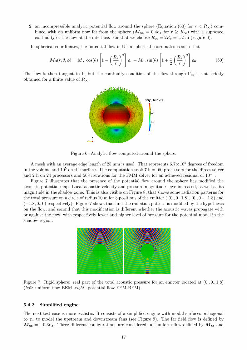
2. an incompressible analytic potential flow around the sphere (Equation (60) for r < R∞) com-bined with an uniform flow far from the sphere (M∞ = 0.4ez for r ≥ R∞) with a supposedcontinuity of the flow at the interface. For that we choose R∞ = 2Rs = 1.2 m (Figure 6).

In spherical coordinates, the potential flow in Ωi in spherical coordinates is such that

M0(r, θ, φ) = M∞ cos(θ)

[1−

(Rsr

)3]er −M∞ sin(θ)

[1 +

1

2

(Rsr

)3]eθ. (60)

The flow is then tangent to Γ, but the continuity condition of the flow through Γ∞ is not strictlyobtained for a finite value of R∞.

Figure 6: Analytic flow computed around the sphere.

A mesh with an average edge length of 25 mm is used. That represents 6.7×105 degrees of freedomin the volume and 105 on the surface. The computation took 7 h on 60 processors for the direct solverand 2 h on 24 processors and 568 iterations for the FMM solver for an achieved residual of 10−6.

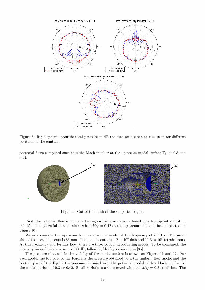
Figure 7 illustrates that the presence of the potential flow around the sphere has modified theacoustic potential map. Local acoustic velocity and pressure magnitude have increased, as well as itsmagnitude in the shadow zone. This is also visible on Figure 8, that shows some radiation patterns forthe total pressure on a circle of radius 10 m for 3 positions of the emitter ( (0., 0., 1.8), (0., 0.,−1.8) and(−1.8, 0., 0) respectively). Figure 7 shows that first the radiation pattern is modified by the hypothesison the flow, and second that this modification is different whether the acoustic waves propagate withor against the flow, with respectively lower and higher level of pressure for the potential model in theshadow region.

Figure 7: Rigid sphere: real part of the total acoustic pressure for an emitter located at (0., 0., 1.8)(left : uniform flow BEM, right : potential flow FEM-BEM).

5.4.2 Simplified engine

The next test case is more realistic. It consists of a simplified engine with modal surfaces orthogonalto ez to model the upstream and downstream fans (see Figure 9). The far field flow is defined byM∞ = −0.3ez. Three different configurations are considered: an uniform flow defined by M∞ and

17

’

Figure 8: Rigid sphere: acoustic total pressure in dB radiated on a circle at r = 10 m for differentpositions of the emitter .

potential flows computed such that the Mach number at the upstream modal surface ΓM is 0.3 and0.42.

Figure 9: Cut of the mesh of the simplified engine.

First, the potential flow is computed using an in-house software based on a fixed-point algorithm[39, 25]. The potential flow obtained when MM = 0.42 at the upstream modal surface is plotted onFigure 10.

We now consider the upstream fan modal source model at the frequency of 200 Hz. The meansize of the mesh elements is 83 mm. The model contains 1.2 × 106 dofs and 11.8 × 106 tetrahedrons.At this frequency and for this flow, there are three to four propagating modes. To be compared, theintensity on each mode is set to 100 dB, following Morfey’s convention [35].

The pressure obtained in the vicinity of the modal surface is shown on Figures 11 and 12. Foreach mode, the top part of the Figure is the pressure obtained with the uniform flow model and thebottom part of the Figure the pressure obtained with the potential model with a Mach number atthe modal surface of 0.3 or 0.42. Small variations are observed with the MM = 0.3 condition. The

18

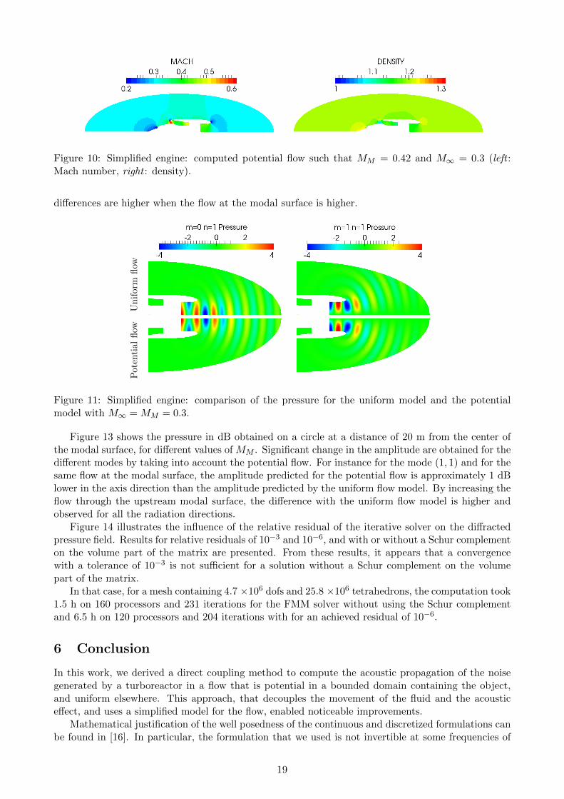
Figure 10: Simplified engine: computed potential flow such that MM = 0.42 and M∞ = 0.3 (left :Mach number, right : density).

differences are higher when the flow at the modal surface is higher.

Un

iform

flow

Pot

enti

alfl

ow

Figure 11: Simplified engine: comparison of the pressure for the uniform model and the potentialmodel with M∞ = MM = 0.3.

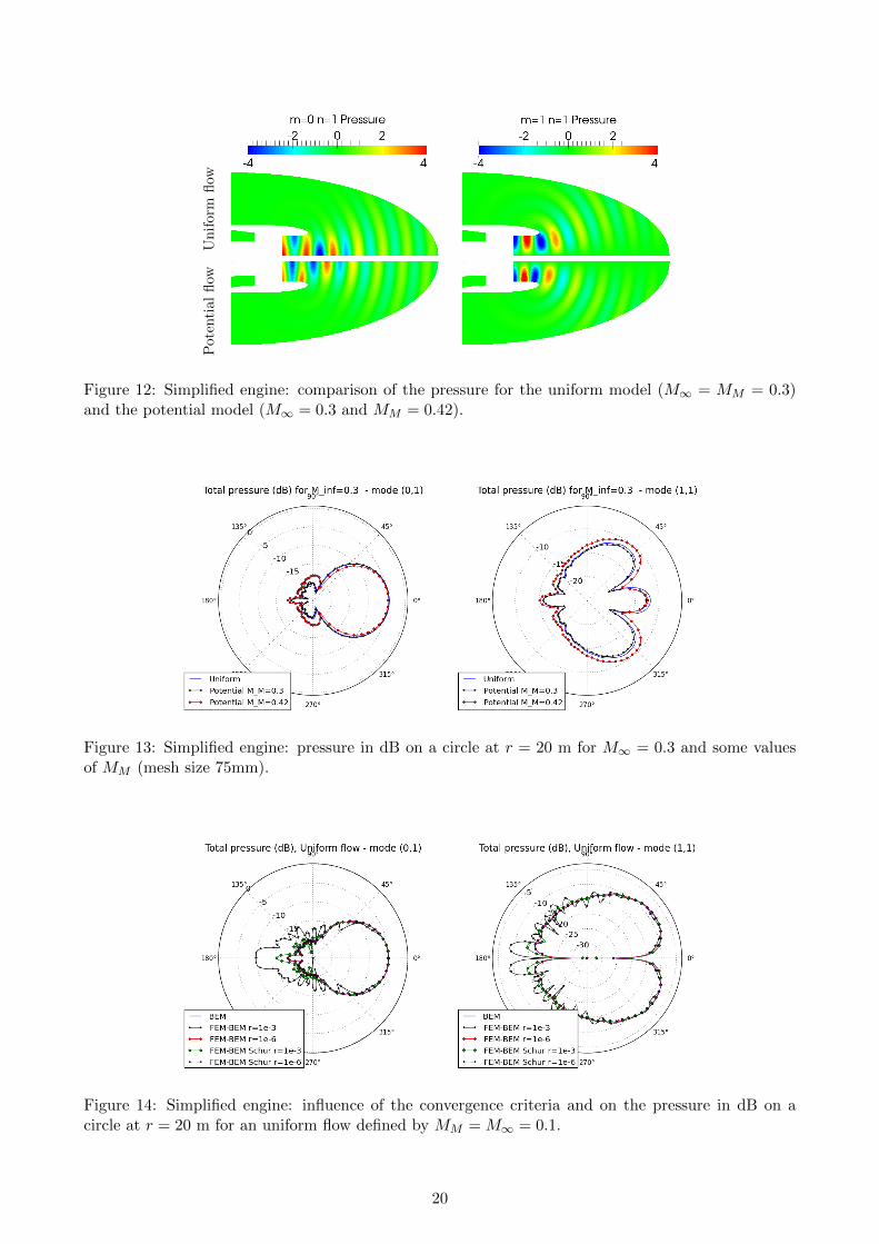
Figure 13 shows the pressure in dB obtained on a circle at a distance of 20 m from the center ofthe modal surface, for different values of MM . Significant change in the amplitude are obtained for thedifferent modes by taking into account the potential flow. For instance for the mode (1, 1) and for thesame flow at the modal surface, the amplitude predicted for the potential flow is approximately 1 dBlower in the axis direction than the amplitude predicted by the uniform flow model. By increasing theflow through the upstream modal surface, the difference with the uniform flow model is higher andobserved for all the radiation directions.

Figure 14 illustrates the influence of the relative residual of the iterative solver on the diffractedpressure field. Results for relative residuals of 10−3 and 10−6, and with or without a Schur complementon the volume part of the matrix are presented. From these results, it appears that a convergencewith a tolerance of 10−3 is not sufficient for a solution without a Schur complement on the volumepart of the matrix.

In that case, for a mesh containing 4.7 ×106 dofs and 25.8 ×106 tetrahedrons, the computation took1.5 h on 160 processors and 231 iterations for the FMM solver without using the Schur complementand 6.5 h on 120 processors and 204 iterations with for an achieved residual of 10−6.

6 Conclusion

In this work, we derived a direct coupling method to compute the acoustic propagation of the noisegenerated by a turboreactor in a flow that is potential in a bounded domain containing the object,and uniform elsewhere. This approach, that decouples the movement of the fluid and the acousticeffect, and uses a simplified model for the flow, enabled noticeable improvements.

Mathematical justification of the well posedness of the continuous and discretized formulations canbe found in [16]. In particular, the formulation that we used is not invertible at some frequencies of

19

Un

ifor

mfl

owP

ote

nti

alfl

ow

Figure 12: Simplified engine: comparison of the pressure for the uniform model (M∞ = MM = 0.3)and the potential model (M∞ = 0.3 and MM = 0.42).

Figure 13: Simplified engine: pressure in dB on a circle at r = 20 m for M∞ = 0.3 and some valuesof MM (mesh size 75mm).

Figure 14: Simplified engine: influence of the convergence criteria and on the pressure in dB on acircle at r = 20 m for an uniform flow defined by MM = M∞ = 0.1.

20

the source. These resonant frequencies are not physical, since the considered boundary value problemalways has a unique solution. A combined field integral equations method can be derived to recoverwell-posedness at all the frequencies. Such a method has been implemented in our code [16].

The method has been implemented for generic 3D configurations. Complementary tests have tobe conducted to catch the limitation of the potential assumption. However, now that the couplinghas been carried out, and considering that the uniform flow assumption is reasonable far from theobject, we can easily enrich the physics of the problem by considering more complex flows in theinterior domain (e.g. rotational flow leading to the Galbrun equation [11]), or other boundary condi-tion. Measurement campaigns are under analysis, and comparisons with our numerical model will bepresented as soon as possible in collaboration with the team responsible for these measurements.

A Appendix

A.1 Alternative computation of the coupling integral term IM (11)

In the same fashion as the exterior problem, it is possible to transform the modal problem (39) torecover the classical Helmholtz equation by introducing a Prandtl–Glauert transformation associatedto MM (this is the case in ACTIPOLE).

Remark A.1. In what follows, we note by ·M the objects and operators transformed by the Prandtl–Glauert transformation associated to MM (normals, geometry, derivatives).

The waveguide is still supposed oriented along a local axis ezM and with the uniform flow MM .

As ΓM is orthogonal to ezM , we suppose zM |ΓM

M= 0. The flow MM is then parallel to ezM .

In ΩMM

, the transformed acoustic potential is decomposed into an incident and a diffracted

potential: ϕM := ϕincM

+ ϕdiffM

, both satisfying

∆M ϕinc,diffM

+ kMM 2ϕinc,diff

M

= 0, in ΩMM. (61)

The incident potential is known, whereas the diffracted potential is unknown. The followingdecomposition holds [36, 13]:

ϕincM

(xM , yM , zM ) =∑(ι)

αιM vι

M (xM , yM ) exp

(ik+ι

MzM)

in ΩMM,

ϕdiffM

(xM , yM , zM ) =∑(ι)

βιMvιM (xM , yM ) exp

(ik−ι

MzM)

in ΩMM,

(62)

with ι a discrete index and where αιM and βι

Mare the incident and diffracted modal coefficients. The

basis functions vιM constitute an orthonormal modal basis function.

For instance for a cylindrical duct of radius R, ι corresponds to a couple of indices (m,n) ∈ (Z×N∗)and the functions vι

M are defined in polar coordinates by [36, 13] by

vιM(rM , θM

)= vm,n

M(rM , θM

)= Vm,n

MJm

(rm,nR

rM)

exp(im θM

), (63)

with rm,n the n-th zero of the derivative of m-th Bessel function of the first kind Jm, Vm,nM

thenormalization factor such that

∫ΓM

M vιM = 1, and

k±ιM

= k±mnM

= ±√(

kMM)2

−(rm,nR

)2, for propagating modes (k±mn

M∈ R), (64)

k±ιM

= k±mnM

= ±i√(rm,n

R

)2−(kM

M)2

, for evanescent modes (k±mnM∈ C). (65)

21

Based on this decomposition, the expression of the Dirichlet-to-Neumann ΛMM

operator is [10, 31]:

∇MϕM · nM = ΛM

M (ϕM)

:=∑(ι)

(αιM Y +

ι

M+ βι

MY −ι

M)vι on ΓM

M, (66)

with Y ±ιM

= −ik±ιM

. Similarly to Section 3.3, by using the Prandtl–Glauert transformation associatedto MM , we infer

IM (ϕi, ϕt) = −JMρMρ∞

∫ΓM

M∇MϕiM· nM ϕMt (67)

= −JMρMρ∞

∫ΓM

MΛM

M(ϕiM)ϕMt. (68)

Then, using the Dirichlet-to-Neumann operator (66), we obtain

IM (ϕi, ϕt) = −JMρMρ∞

∑(ι)

[αιM Y +

ι

M+ βι

MY −ι

M] ∫

ΓMMvιM ϕMt. (69)

However, to carry out a coupling between unknown functions written in the same variables, the in-tegral IM must be expressed in terms of quantities transformed by the Prandtl–Glauert transformationassociated to M∞. Using the results obtained in Section 3.3, we have that

JM

∫ΓM

MgM (xM ) hM (xM ) =

∫ΓM

1

KMM

(x)g(x) h(x) =

∫ΓM

J∞K∞(x)

KMM

(x)g(x) h(x),

where KMM

and K∞ are defined in equation (26).Equation (69) becomes

IM (ϕi, ϕt) = −J∞ρMρ∞

∑(ι)

[αιM Y +

ι

M+ βι

MY −ι

M] ∫

ΓM

K∞(x)

KMM

(x)vι ϕt. (70)

If MM and M∞ are colinear, there holds

K∞

KMM

=

√1−M2

M

1−M2∞,

and otherwise, denoting α = M∞ · nM ,

K∞

KMM

=

√[(1 + C∞α2)(1 + CM

MM2M )]2

+ C2∞α

2(M2∞ − α2).

Acknowledgments

This work takes part in the AEROSON project, financed by the ANR (French National ResearchAgency). The authors would like to express their gratitude to Toufic Abboud (IMACS), Patrick Joly(INRIA) and Guillaume Sylvand (Airbus Group) for fruitful discussions and to Emilie Peynaud andFrancois Madiot for their work during their internship at Airbus Group.

References

[1] S. Abarbanel, D. Gottlieb, and J. S. Hesthaven. Well-posed perfectly matched layers for advectiveacoustics. Journal of Computational Physics, 154:266–283, 1999.

22

[2] T. Abboud, P. Joly, J. Rodrıguez, and I. Terrasse. Coupling discontinuous Galerkin methods andretarded potentials for transient wave propagation on unbounded domains. Journal of Computa-tional Physics, 230:5877–5907, 2011.

[3] P. R. Amestoy, I. S. Duff, J. Koster, and J.-Y. L’Excellent. A fully asynchronous multifrontalsolver using distributed dynamic scheduling. SIAM Journal on Matrix Analysis and Applications,23(1):15–41, 2001.

[4] P. R. Amestoy, A. Guermouche, J.-Y. L’Excellent, and S. Pralet. Hybrid scheduling for theparallel solution of linear systems. Parallel Computing, 32(2):136–156, 2006.

[5] R. Amiet and W. R. Sears. The aerodynamic noise of small-perturbation subsonic flows. Journalof Fluid Mechanics, 44:pp. 227–235, 1970.

[6] R.J. Astley and J.G. Bain. A three-dimensional boundary element scheme for acoustic radiationin low mach number flows. Journal of Sound and Vibration, 109(3):445 – 465, 1986.

[7] M. Beldi and F. S. Monastir. Resolution of the convected Helmholtz’s equation by integralequations. The Journal of the Acoustical Society of America, 103:2972, 1998.

[8] J. P. Berenger. A perfectly matched layer for the absorption of electromagnetic waves. Journalof Computational Physics, 114:185–200, 1994.

[9] J. Bielak and R. C. Mac Camy. Symmetric Finite Element and Boundary Integral CouplingMethods for Fluid-Solid Interaction. Quarterly of Applied Mathematics, 49:107–119, 1991.

[10] A.-S. Bonnet-Ben Dhia, L. Dahi, E. Luneville, and V. Pagneux. Acoustic diffraction by a platein a uniform flow. Mathematical Models and Methods in Applied Sciences, 12(05):625–647, 2002.

[11] A.-S. Bonnet-Ben Dhia, J.-F. Mercier, F. Millot, S. Pernet, and E. Peynaud. Time-HarmonicAcoustic Scattering in a Complex Flow: a Full Coupling Between Acoustics and Hydrodynamics.Communications in Computational Physics, 11(2):555–572, 2012.

[12] E. J Brambley. Well-posed boundary condition for acoustic liners in straight ducts with flow.AIAA journal, 49(6):1272–1282, 2011.

[13] M. Bruneau and T. Scelo. Fundamentals of Acoustics. ISTE, 2006.

[14] A. J. Burton and G. F. Miller. The application of integral equation methods to the numericalsolution of some exterior boundary-value problems. Proceedings of the Royal Society of London.A. Mathematical and Physical Sciences, 323(1553):201–210, 1971.

[15] B. Carpentieri, I. S. Duff, L. Giraud, and G. Sylvand. Combining fast multipole techniques andan approximate inverse preconditioner for large electromagnetism calculations. SIAM Journal onScientific Computing, 27:774–792, 2005.

[16] F. Casenave, A. Ern, and G. Sylvand. Coupled BEM-FEM for the convected Helmholtz equa-tion with non-uniform flow in a bounded domain. Journal of Computational Physics, 257, PartA(0):627–644, 2014.

[17] C. J. Chapman. Similarity variables for sound radiation in a uniform flow. Journal of Sound andVibration, 233(1):157 – 164, 2000.

[18] P. G. Ciarlet. The Finite Element Method for Elliptic Problems. North Holland, Amsterdam,1978.

[19] M. Costabel. Symmetric methods for the coupling of finite elements and boundary elements.Preprint. Fachbereich Mathematik. Technische Hochschule Darmstadt. Fachber., TH, 1987.

23

[20] A. Craggs. An acoustic finite element approach for studying boundary flexibility and soundtransmission between irregular enclosures. Journal of Sound and Vibration, 30:343–357, 1973.

[21] A. Delnevo. Code ACTI3S harmonique : Justification Mathematique. Technical report, EADSCCR, 2001.

[22] A. Delnevo. Code ACTI3S, Justifications Mathematiques : partie II, presence d’un ecoulementuniforme. Technical report, EADS CCR, 2002.

[23] A. Delnevo, S. Le Saint, G. Sylvand, and I. Terrasse. Numerical methods: Fast multipole methodfor shielding effects. 11th AIAA/CEAS Aeroacoustics Conference, pages 2005–2971, 2005. Mon-terey.

[24] F. Dubois, E. Duceau, F. Marechal, and I. Terrasse. Lorentz transform and staggered finitedifferences for advective acoustics. Technical report, EADS and arXiv:1105.1458, 2002.

[25] S. Duprey. Analyse Mathematique et Numerique du Rayonnement Acoustique des Turboreacteurs.PhD thesis, EADS-CRC ; Institut Elie Cartan-Universite Poincare Nancy, 2005.

[26] W. Eversman. Approximation for thin boundary layers in the sheared flow duct transmissionproblem. The Journal of the Acoustical Society of America, 53(5):1346–1350, 1973.

[27] L. Giraud, J. Langou, and G. Sylvand. On the parallel solution of large industrial wave propaga-tion problems,. Journal of Computational Acoustics, 14:83–111, 2006.

[28] H. Glauert. The effect of compressibility on the lift of an aerofoil. Proceedings of the Royal Societyof London. Series A, Containing Papers of a Mathematical and Physical Character, 118(779):pp.113–119, 1928.

[29] F. H. Harlow, J. E. Welch, J. P. Shannon, and B. J. Daly. The MAC method. Technical report,Los Alamos Scientific Laboratory, march 1966.

[30] C. Johnson and J. C. Nedelec. On the coupling of boundary integral and finite element methods.Mathematics of Computation, 35(152):1063–1079, 1980.

[31] G. Legendre. Rayonnement acoustique dans un fluide en ecoulement : analyse mathematique etnumerique de l’equation de Galbrun. These, ENSTA ParisTech, September 2003.

[32] V. Levillain. Couplage elements finis-equations integrales pour la resolution des equations deMaxwell en milieu heterogene. PhD thesis, These Ecole Polytechnique, 1991.

[33] S. Lidoine. Approches theoriques du probleme du rayonnement acoustique par une entree d’air deturboreacteur: Comparaisons entre differentes methodes analytiques et numeriques. PhD thesis,Ecole centrale de Lyon, 2002.

[34] W.C.H. McLean. Strongly Elliptic Systems and Boundary Integral Equations. Cambridge Uni-versity Press, 2000.

[35] C.L. Morfey. Acoustic energy in non-uniform flows. Journal of Sound and Vibration, 14(2):159 –170, 1971.

[36] P. M. Morse and K. Ingard. Theoretical acoustics. McGraw-Hill Book Co., 1968.

[37] MK Myers. On the acoustic boundary condition in the presence of flow. Journal of Sound andVibration, 71(3):429–434, 1980.

[38] J.C. Nedelec. Acoustic and Electromagnetic Equations: Integral Representations for HarmonicProblems, volume 144 of Applied Math. Sciences. Springer, 2001.

[39] J. Periaux. Three dimensional analysis of compressible potential flows with the finite elementmethod. International Journal for Numerical Methods in Engineering, 9(4):775–831, 1975.

24

[40] J. W. S. Rayleigh. The theory of sound. Macmillan and co, London, 1877.

[41] V. Rokhlin. Rapid solution of integral equations of classical potential theory. Journal of Compu-tational Physics, 60:187–207, 1985.

[42] A. Hirschberg S. W. Rienstra. An Introduction to Acoustics. Eindhoven University of Technology,2004.

[43] H. A. Schenck. Improved Integral Formulation for Acoustic Radiation Problems. The Journal ofthe Acoustical Society of America, 44:41–58, 1968.

[44] A. Sommerfeld. Die Greensche Funktionen der Schwingungsgleichung. Jahresber. Deutsch. Math.Verein., 21:309–353, 1912.

[45] G. Sylvand. La methode multipole rapide en electromagnetisme. Performances, parallelisation,applications. PhD thesis, Ecole des Ponts ParisTech, 2002.

[46] A. Taflove. Computational Electrodynamics: The Finite-Difference Time-Domain Method. ArtechHouse, Norwood, MA, 1995.

[47] J. Virieux. PSV-wave propagation in heterogeneous media: velocity-stress finite differencemethod. Geophysics, 51:889–901, 1986.

[48] M.C.M. Wright. Lecture Notes On The Mathematics Of Acoustics. Imperial College Press, 2005.

[49] F. Zhang. The Schur Complement and Its Applications. Numerical Methods and Algorithms.Springer, 2005.

[50] O. C. Zienkiewicz, D. W. Kelly, and P. Bettess. The coupling of the finite element methodand boundary solution procedures. International Journal for Numerical Methods in Engineering,11:355–375, 1977.

25