boundary layer response to a change in surface roughness layer response to a... · boundary-layer...
TRANSCRIPT

The University of Reading
Department of Meteorology
Boundary-layer response to a change in surface
roughness.
James Benson
A dissertation submitted in partial fulfilment of the requirement
for the degree of MSc Applied Meteorology
15th August 2005

ii
Acknowledgements Many thanks to my supervisor Janet Barlow for all the invaluable help and guidance during
this project. A special thanks to Frauke Pascheke who spent many days teaching me the ways
of Reading wind tunnel and who was always had time (and answers) for my questions. Also
thanks to the lab technicians for keeping the equipment working.

iii
Abstract The Earth’s surface heterogeneity means that airflow is continually encountering changes in
surface roughness. Previous research into the effects of these changes has shown the
formation of an internal boundary layer, changing shear stresses and the turbulent response to
such a change. This experiment uses a wind tunnel and hot wire anemometry to examine these
aspects for a single simplified roughness change. The difficulties of investigating such
features in a small wind tunnel are addressed, with consideration of surface morphology and
applicability to full scale situations.
While most previous studies have considered the effect of a change in roughness length, most
have neglected the effect of changing displacement height. In this experiment two surface
roughness changes are investigated, both consisting of a change from upstream 3D Lego™
type roughness elements to downstream 2D bar type roughness. The downstream surface
roughness bar height to canyon width ratio is different in each roughness change case
providing different surface roughness and displacement height parameters. One surface
provides a smooth to rough change while the other provides a rough to smooth change. The
effects of both roughness changes are acceleration of the flow and reduction in shear stress
over the initial bar of downstream roughness. Downstream of the roughness change the shear
stress varies periodically with fetch, has a wavelength equal to the bar spacing and an
amplitude that decreases with height.
Velocity profiles are found to indicate the formation of an IBL although there is insufficient
fetch for an equilibrium layer to form. However by using morphometric analysis, surface
parameters are estimated allowing IBL height growth theories to be compared with the IBL
heights determined by gradient changes in the measured wind profile. The results of this
experiment compare favourably with some theories although further experiments would be
needed to confirm this is the case at longer downwind fetches. However over urban areas
there is likely to be insufficient fetch for these conventional theories to be correctly applied. It
is also found that within the fetch range considered in this experiment the displacement height
is shown to be significant factor in determining the effect of a roughness change.

iv
Contents Acknowledgements ii
Abstract iii
Contents iv
List of figures and tables vi List of figures vi
List of tables vii
Mathematical Symbols used viii
1. Introduction 1
1.1 Motivation 1
1.2 Objectives 1
1.3 Structure 1
2. Theory 2
2.1 Turbulent flow over a rough surface. 2
2.2 Effect of a roughness change 4
2.2.1 Introduction 4
2.2.2 IBL depth 6
2.2.3 Equilibrium layer depth 7
2.2.4 Morphometric surface analysis 8
2.2.5 Development of stress after a roughness change 12
2.3 Wind tunnel theory 14
2.3.1 Turbulence 14
2.3.2 Wind profiles 17
2.3.3 Blockage 17
3 Wind tunnel setup 18
3.1 Apparatus 18
3.1.1 Roughness element setup 19
3.2 Measurement method 21
3.2.1 Overview 21
3.2.2 The pitot tube 21
3.2.3 The hot wire 22
3.2.4 The crossed hot wire 24

v
3.3 Measuring procedure 24
3.4 Sources of error 25
3.4.1 Temperature 25
3.4.2 Calibration error 25
3.4.3 Pressure variations 26
3.4.4 Probe positioning 26
3.4.5 High turbulence intensity errors 26
4 Results and analysis 27
4.1 Morphometric surface roughness analysis results 27
4.1.1 Lego™ surface roughness 27
4.1.2 2D bar type roughness 28
4.2 Profiles above upstream Lego™ roughness 29
4.2.1 Introduction 29
4.2.2 Upwind boundary layer structure 31
4.2.3 Turbulence over Lego™ surface 35
4.2.4 Turbulence spectra 37
4.3 Profiles over R1 roughness type 38
4.3.1 Initial flow disturbance 39
4.3.2 Shear stress 40
4.3.3 Turbulence response 43
4.4 R2 roughness type 46
4.4.1 Velocity and shear stress 46
4.4.2 Turbulent Intensity 49
4.4.3 IBL height. 51
4.4.4 Shear stress overshoot 54
5 Conclusions 55
Appendices 59
Appendix 1. Location of profile measurements over Lego™ surface roughness 59
Appendix 2. Rejected Lego™ wind profiles. 59
Appendix 3. Change in normalisation wind speed with fetch 60
Appendix 4. Log law fit using u* (IS) and average velocity profile over Lego™ 61
Appendix 5. Errors in mean velocity and shear stress measurements 61
References 62

vi
List of figures and tables List of figures Figure 1 Wind profile above a rough surface
Figure 2 Effect of a surface roughness change
Figure 3 Idealised morphometric surface roughness dimensions
Figure 4 Displacement height for 2D bar type roughness
Figure 5 Shear stress overshoot
Figure 6 Shear stress undershoot
Figure 7 Wind tunnel setup
Figure 8 Spires used to initiate turbulence
Figure 9 Lego™ roughness element dimensions
Figure 10 Downstream surface roughness types
Figure 11 Equipment setup
Figure 12 Wind and turbulent intensity profiles over Lego™ surface
Figure 13 Normalised shear stress profiles over Lego™ surface
Figure 14 Turbulent intensity components, σu/U, σw/U and σw/σu over Lego™ surface
Figure 15 Turbulent intensity components, σu/U, σv/U and σv/σu over Lego™ surface
Figure 16 Normalised spectral energy density distributions over Lego™ surface
Figure 17 Wind profiles after change in roughness from Lego™ to R1 type roughness
Figure 18 Flow disturbance caused by roughness change from Lego™ to R1
Figure 19 Normalised shear stress variations with fetch over R1 type roughness
Figure 20 Normalised shear stress profiles over R1 type roughness
Figure 21 u* values variation with fetch over R1 type roughness
Figure 22 Turbulent intensity u component over R1 type roughness
Figure 23 Turbulent intensity w component over R1 type roughness
Figure 24 Wind profiles after change in roughness from Lego™ to R2 type roughness
Figure 25 Normalised shear stress variations with fetch over R2 type roughness
Figure 26 Normalised shear stress profiles over R2 type roughness.
Figure 27 u* values variation with fetch over R2 type roughness
Figure 28 Turbulent intensity u component over R2 type roughness
Figure 29 Turbulent intensity w component over R2 type roughness
Figure 30 IBL growth after a change in surface roughness from Lego™ to R2

vii
Figure 31 IBL growth after a change in surface roughness from Lego™ to R2 including
consideration of displacement height
Figure 32 Shear stress overshoot comparison with theory
Figure 1A Location of profile measurements over Lego™ surface roughness
Figure 2A Rejected profiles over Lego™ surface roughness
Figure 3A Change in normalisation wind speed with fetch over Lego™
Figure 3B Change in normalisation wind speed with fetch over change in surface
roughness from Lego™ to R1
Figure 4A Log law fit using u*(IS) and average velocity profile over Lego™ surface
List of tables Table 1 Coefficient for spectral density functions derived from atmospheric studies
Table 2 Geometric parameters for Lego™ roughness used in wind tunnel
Table 3 Log law parameters derived from surface form for roughness types
Table 4 Downstream roughness parameters
Table 5 u*/upref , z01 and d1 values
Table 6 Comparison table of u* (IS)/upref values
Table 7 Differences between over bar and over canyon normalised shear stress
Table 1A Errors in mean velocity and shear stress measurements

viii
Mathematical Symbols used a - Overheat Ratio AF - Frontal area (m) Ap - Element plan area (m) AT - Lot area (m) CD - Drag Coefficient d - Displacement height (m) Dx,y - Lot dimensions (x or y axis) (m) f - Frequency (Hz) fred - Reduced Frequency (Hz) k - Von Karman Constant Km – Turbulent exchange coefficient for momentum. (m2s-1) Lx,y - Element dimeansions (x or y axis) (m) M - Roughness change parameter Ra - Resistance of wire at ambient temperature (Ta) (Ω) Rc – Resistance of probe cable (Ω) Re* - Roughness Reynolds number Rp – Resistance of probe (including prongs) (Ω) Rs – Resistances of connection leads in probe support (Ω) Rw - Resistance of heated wire at temperature (Tw) Suu - Spectral density function T20 – Reference temperature (20oC) u* - Friction velocity (ms-1) u, v, w - Velocity (x, y, z) (ms-1) xF - Fetch required for flow to be in equilibrium at height z (m) z - Height (m) z0 - Roughness length (m) zH - Element height (m) α20 – Temperature coefficient of resistance at 20oC (%K-1) β - Drag correction factor δ - Boundary layer depth (m) δe - Inner equilibrium Layer height (m) δi - Internal boundary Layer height (m) λF - Frontal area index λP - Plan areal fraction ν - Kinematic viscosity (m2s-1) ρ - Density (kgm-3) τ - Turbulent momentum flux or stress (kgs-2) Ф - Blockage Coefficient e - Turbulent Kinetic Energy (Jkg-1) u - Mean wind velocity (ms-1) upref - Mean wind velocity measured by reference pitot tube (ms-1) uθ - Mean wind velocity measured with wind incident at θ to sensor (ms-1)

1
1. Introduction 1.1 Motivation The boundary layer is the part of the atmosphere directly influenced by the surface. In the
horizontal plane the surface characteristics are almost constantly changing, resulting in
airflow that has partially adjusted to the characteristics of many upstream surfaces. These
changes can be gradual or sharp and the angle at which the wind approaches these changes is
usually changing due to, for example, the prevailing synoptic conditions. In order to simplify
the complexity of real life surface roughness changes a single roughness change will be setup
in a wind tunnel controlled environment. It is in the boundary layer where surface based
meteorological measurements are taken, and so it is essential to understand the effect of
upwind surfaces to the measurement site on the results obtained. Also the dispersion of
pollutants from the surface is crucially dependent on turbulence and other flow characteristics
of the boundary layer, whose structure is in turn determined by the nature of the upwind
surfaces.
1.2 Objectives To investigate the effect on airflow of a change in surface roughness (and/or displacement
height) using a wind tunnel. Aspects of this study include surface stress, velocity, turbulence
and comparison with the features of wind tunnel, theoretical and modelling results of other
authors. Standard single hot wire and crossed hot wire anemometry have been used in a small
wind tunnel at Reading University. Upstream roughness was created by using Lego™ blocks
and downstream roughness by street canyon type laterally arranged square bars.
1.3 Structure This report begins with a review of applicable theory of flow over rough surfaces, the effect
of roughness changes and the characterisation of a wind tunnel generated boundary layer
(section 2). The experimental setup is then discussed in section 3, with a review of
morphometric surface analysis methods, measurement methods and sources of error. Section
4 then presents the results and discussion, followed by the conclusions in section 5.

2
2. Theory The aspects of theory that are related to this experiment are examined in this section. If the
effects of a surface roughness change are to be understood it is necessary to understand the
structure of the approaching flow before the roughness is encountered. Therefore the basic
theory of flow over a rough surface is summarised in this section. The theoretical effect of a
roughness change is then considered with sections on internal boundary layer (IBL) and
equilibrium layer depth, shear stress development and the application of morphometric
methods of surface analysis for estimation of surface parameters. The theoretical aspects of
creating a boundary layer in a wind tunnel are also considered.
2.1 Turbulent flow over a rough surface. Before considering the effect of a change of roughness it is necessary to examine the flow
structure over a uniform area of rough surface. Rough flow is when the shear stress is
dominated by the drag of the roughness elements as compared to smooth flow where the shear
stress is dominated by viscosity (Raupach et al., 1991). The structure of flow over a rough
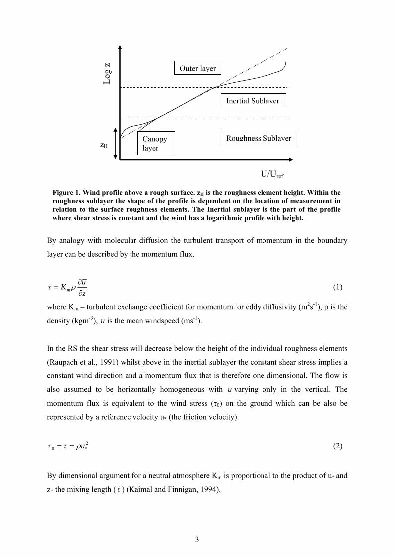
surface is usually identified by the following layers (Figure 1);
1) A roughness sublayer (RS) where the velocity is horizontally inhomogeneous as
the airflow is influenced by the individual roughness elements.
2) A inertial sublayer (IS) within which the flow is horizontally homogeneous and the
wind varies only with height (z).
The depth of the RS is dependent on surface geometry but is usually 2-5 times the height of
the roughness elements (Cheng and Castro, 2002). Within the RS there exists a canopy layer
below the height of the elements themselves, where the flow is spatially inhomogeneous. The
shear stress profile in the RS is also horizontally inhomogeous, while in the IS above the
shear stress is approximately constant with height (to 10% (Oke, 1987)) and horizontally
homogenous, which is one assumption for the correct application of the log wind law.
3
By analogy with molecular diffusion the turbulent transport of momentum in the boundary
layer can be described by the momentum flux.
zuKm ∂∂
= ρτ (1)
where Km – turbulent exchange coefficient for momentum. or eddy diffusivity (m2s-1), ρ is the
density (kgm-3), u is the mean windspeed (ms-1).
In the RS the shear stress will decrease below the height of the individual roughness elements
(Raupach et al., 1991) whilst above in the inertial sublayer the constant shear stress implies a
constant wind direction and a momentum flux that is therefore one dimensional. The flow is
also assumed to be horizontally homogeneous with u varying only in the vertical. The
momentum flux is equivalent to the wind stress (τ0) on the ground which can be also be
represented by a reference velocity u* (the friction velocity).
2*0 uρττ == (2)
By dimensional argument for a neutral atmosphere Km is proportional to the product of u* and
z- the mixing length ( l ) (Kaimal and Finnigan, 1994).
Log
z
U/Uref
Roughness Sublayer
Inertial Sublayer
Outer layer
Figure 1. Wind profile above a rough surface. zH is the roughness element height. Within the roughness sublayer the shape of the profile is dependent on the location of measurement in relation to the surface roughness elements. The Inertial sublayer is the part of the profile where shear stress is constant and the wind has a logarithmic profile with height.
Canopy layer zH

4
zkuK m *= (3)
k is the constant of proportionality also known as the Von Karman constant ≈ 0.4.
Thus by substitution of equation 2 and 3 into 1 to give the wind shear and then integrating.
⎟⎟⎠
⎞⎜⎜⎝
⎛=
0
* lnzz
ku
u (4)
Where z0 is known as the roughness length, describing the height where the profile
extrapolates to zero velocity. Depending on the nature of the surface there is a modification to
the log law to account for the displacement for the flow by the surface elements.
⎟⎟⎠
⎞⎜⎜⎝
⎛ −=
0
* lnz
dzku
u (5)
This is also equivalent to the height at which the mean drag on the surface appears to act
(Jackson, 1981).
A direct measure of the momentum flux is given by.
''wuρτ −= (6)
Where 'u is the fluctuating component of the wind in the direction of mean flow, 'w is the
fluctuating component of the wind normal and in the vertical. ''wu is the covariance of the
fluctuating parts. This is known as the Reynolds stress and is the mean force per unit area
imposed on the mean flow by turbulent fluctuations,
2.2 Effect of a roughness change 2.2.1 Introduction
This experiment is concerned with the response of a turbulent boundary layer to a change of
surface roughness. This has been studied extensively both by wind tunnel (e.g. Antonia and
Luxton, 1971; Mulhearn, 1978; Pendergrass and Arya, 1984; Cheng and Castro, 2002) and in
the field (e.g. Bradley, 1968). The effect of a roughness change can be characterised by:

5
1) An Internal Boundary layer (IBL) developing over the new surface, growing in
height with increasing distance downwind from the change.
2) A development of wind profiles, shear stress within this internal boundary layer as
the flow adjusts to the new surface.
Most studies have considered a step change in surface roughness in a neutral boundary layer,
which is also the topic of this study. A diagram of IBL growth is shown in Figure 2a. A
typical wind profile at some distance x downwind of the roughness change is shown in Figure
2b. Above the IBL the flow is characteristic of the upwind surface, while below it is affected
by both the downstream and upstream roughness in the transition region. Below this is the
inner equilibrium layer where the flow has adjusted to the new surface.
x x = 0 ),( 0101 zτ
δi (x)
)),(( 0202 zxτ
δe (x)
z
Figure 2. Effect of a change in surface roughness. (a) The growth of an IBL downstream of a change in surface roughness (x=0). IBL depth is δi(x), inner equilibrium layer depth δe(x). (b) Velocity profiles before and after a change in roughness from smooth to rough. δi is the IBL depth by the extension of the downstream profile to intersection with the upwind profile. δ2i is the IBL depth as determined by the point of inflection.
Transition layer
⎟⎟⎠
⎞⎜⎜⎝
⎛ −=
01
11*1 ln)(
zdz
kuzu
⎟⎟⎠
⎞⎜⎜⎝
⎛ −=
02
22*2 ln)(
zdz
kuzu
δe
)(zu (ms-1)
z
(a)
(b) δiδ2i
Inflection point

6
2.2.2 IBL depth
One particular difficulty is defining where the top of the IBL is as some authors (Cheng and
Castro, 2002) take this as where the velocity reaches 99% of its upstream value, however 1%
differences may be difficult to measure experimentally. Another method (Mulhearn,1978;
Bradley, 1968; Elliot, 1958) is to take the point in the log plotted profile where the downwind
velocity profile merges into the upwind profile. The exact position of this ‘knee’ point is open
to interpretation as shown by the difference between δi – the intersection point and δ2i – the
point of inflection as shown in Figure 2b. δi gives a higher IBL but is dependent on obtaining
a good log fit in the equilibrium layer which may be may not be that deep depending on fetch
and roughness geometry (see section 2.2.3). The point of inflection method (δ2i) has the
disadvantage of being indistinct in situations where the there are small differences in
downwind and upwind profiles. Antonia and Luxton (1971) argued from theoretical grounds
that plotting u vs. z1/2 gives linear profiles of the upstream and downstream profiles whose
intersection marks the IBL height.
Another method of obtaining the IBL height is via stress measurements, for example the
height where there is a 1% increase compared to the upstream value at the same height for a
SR change. This usually tends to give a larger IBL height in comparison to the velocity
method as stress adjusts faster than velocity profiles.
The evolution of IBL height with fetch has been reviewed by Walmsley (1989) and Savelyev
and Taylor (2005) with comparisons to wind tunnel and field data. They find that there is a
large variation of heights predicted. Elliot (1958) used the following empirical formula;
n
i
zxM
z ⎟⎟⎠
⎞⎜⎜⎝
⎛−==
0202
)03.075.0('δ
δ (7)
where ⎟⎟⎠
⎞⎜⎜⎝
⎛=
01
02lnzz
M describes the ‘strength’ of the roughness change, n = 0.8 and the
subscripts 1 and 2 refer to upstream and downstream respectively. The dependence on M in
this formula is weak and thus this expression is frequently used in an M independent form
M=1 (Walmsley, 1988).
7
n
i
zx
z ⎟⎟⎠
⎞⎜⎜⎝
⎛==
0202
72.0'δ
δ (8)
Elliot’s (1958) formula (equation 7) agrees well with Bradley’s (1968) smooth to rough (SR)
and rough to smooth (RS) transitions, and also Antonia and Luxton's (1972) SR experiment
(Kaimal and Finnigan, 1994). However Antonia and Luxton (1972) found for their rough to
smooth study that the n coefficient was ~ 0.43.
Wood (1982) uses a similar formula, arguing that only the rougher surface is important.
8.0
00
28.0 ⎟⎟⎠
⎞⎜⎜⎝
⎛=
rr
i
zx
zδ
(9)
Where ),max( 01020 zzz r = . It is also noted that Wood (1982) considered his formula only
valid up to δi/δ=0.2 where δ is the depth of the boundary layer in which the IBL develops.
Another approach is to use a ‘diffusion analogy’ approach assuming that the growth of IBL is
analogous to the spread of a passive contaminant (Miyake ,1965; Savelyev and Taylor,
2005). From this reasoning Panofsky and Dutton (1984) obtained the following formula for
IBL depth.
11ln25.1020202
+⎟⎟⎠
⎞⎜⎜⎝
⎛−=
zzzxk ii δδ
(10)
2.2.3 Equilibrium layer depth
The inner equilibrium layer is usually taken as the lowest 10% of the IBL (Kaimal and
Finnigan, 1994), and is a constant stress layer in equilibrium with the new surface. Wieringa
(1993) presents an equation for the fetch needed (xF) to ensure that the flow at height z is in
equilibrium with the new surface based on this 10% assumption.
⎥⎥⎦
⎤
⎢⎢⎣
⎡+⎟
⎟⎠
⎞⎜⎜⎝
⎛⎟⎟⎠
⎞⎜⎜⎝
⎛−
−−= 11)(10ln)(102
02
2
02
202 z
dzz
dzzxF (11)

8
However if there is insufficient fetch then this equilibrium layer may not extend above the RS
and so be difficult to identify due to the spatial inhomogenities in flow caused by the
roughness elements as found by Cheng and Castro (2002). To obtain the log law parameters a
constant stress equilibrium layer is required and so to obtain these for a surface with no such
equilibrium layer a morphometric method of surface analysis can be used.
2.2.4 Morphometric surface analysis
The surface drag depends on the layout and size of the roughness elements, which in turn can
be formulated to give directly the z0 and d parameters. A review of such morphometric
methods is provided by Grimmond and Oke (1999), Macdonald et al. (1998).
These methods consider the geometry as shown in Figure 3 and are divided into 3 general
approaches;
1) Height based.
2) Height and plan areal fraction yx
yx
T
Pp DD
LL
AA
==λ based.
3) Height and frontal area index yx
yH
T
FF DD
Lz
AA
==λ based.
Figure 3. Idealised morphometric surface roughness dimensions.
9
3D roughness geometry
To calculate z0 and d the simplest method of estimation is a ‘rule of thumb’ approach:
Hzz 1.00 = (12a)
Hzd 7.0= (12b)
where coefficients 0.1 and 0.7 are chosen by Grimmond and Oke (1999) as a representation of
results of wind tunnel and field studies. The major limitation of this height based approach is
that it does not take roughness element density into account, but the coefficients can be
changed depending on what surface is being studied.
Early studies by Lettau (1969) used data obtained by from the field experiments of Kutzbach
(1961) that used bushel baskets placed in a regular grid on a frozen lake, giving:
FHzz λ5.00 = (13)
This expression starts to fail when λF increases beyond 20 – 30% (see discussion of
Macdonald et al. 1998) due to the interaction of air flow between each obstacle and
consequent development of a non zero displacement height. Also as it is based on results
obtained using bushel baskets in regular arrangement it is in principle limited to that specific
element type and arrangement.
Counihan (1971) used a height and plan areal fraction method where:
Hp zz )08.008.1(0 −= λ (14a)
Hp zd ]0463.0)4352.1[ −= λ (14b)
These equations describe the results obtained in wind tunnel experiments using Lego™
elements on a Lego™ base board and so has specific application to the current experiment.
Counihan (1971) considered the limits of equation 14(a) to be 25.01.0 << pλ . The lower
limit was chosen because z0 is very dependent on element spacing, and the possibility that
measurements made would be of an elements individual wake flow rather than of the

10
boundary layer flow produced by the roughness elements. Consequently it was found that at
low density arrangements it was possible to determine a z0 for the baseboard and a separate z0
for the roughness elements. In those cases Counihan (1971) presents a spatial average to
ensure that both effects are accounted for. However as considered earlier in section 2 this
spatial inhomogenity is expected in the RS and so z0 and d values should ideally be obtained
from measurements in the IS. Above 0.25 the results obtained were distinctly non linear and
no curve was fitted, although Grimmond and Oke (1999) do fit a curve based on Counihan’s
(1971) results that covers λP =0 to 0.5
H
j
j
jpj zCCz ⎟⎟⎠
⎞⎜⎜⎝
⎛+= ∑
=
=
−10
2
110 λ (14c)
Where C1=0.02677, C2=1.3676, C3=15.98, C4=387.15, C5=-4730, C6=32057, C7=-124308,
C8=-124308, C8=27162, C9=-310534, C10=14444
Macdonald et al. (1998), starting from fundamental principles, derived formulas for z0 and d
(equation 15a,b) that are applicable to higher densities (λP, λF) and which show behaviour
consistent with experiments (Counihan, 1971). For instance, for increasing densities z0 begins
to decline after a peak, as would be expected with the development of skimming flow over the
elements. This method allows for corrections for turbulence, velocity profile, flow incidence
and rounded edges and is considered applicable to both 2D and 3D elements.
( ))1(1 −+= −pH
pzd λα λ (15a)
⎪⎩
⎪⎨⎧
⎪⎭
⎪⎬⎫
⎥⎦
⎤⎢⎣
⎡⎟⎟⎠
⎞⎜⎜⎝
⎛−−⎟⎟
⎠
⎞⎜⎜⎝
⎛−=
− 5.0
20 15.0exp1 FH
D
HH z
dkC
zdzz λβ (15b)
α - An empirical coefficient obtained from evaluation of wind tunnel data
= 4.43 for staggered array of roughness elements (Macdonald, 1998)
= 3.59 for square (regular) array of roughness elements (Macdonald, 1998)
CD - Drag coefficient, depends on dimensions of surface elements (ESDU, 1986)
β - Drag correction factor, accounts for velocity profile shape, turbulence, flow
incidence, rounded edges (ESDU, 1986)
11
2D roughness geometry
There has also been a large amount of research into the effect of flow over 2D bar canyon
type roughness by both modelling (Sini et al., 1996; Leonardi et al., 2003) and by analysis of
wind tunnel experiments (Oke, 1987). The streets are usually considered in terms of their
height to width ratio (=zH/Wx). Oke (1987) describes 3 regimes of flow associated with this
type of roughness;
1) Isolated flow – Bar rows far enough apart for the flow to be the same as that for
isolated buildings for zH/Wx < 0.3.
2) Wake interference flow – Wake from upwind bar interferes with downstream bar’s
flow pattern for 0.3 < zH/Wx < 0.65
3) Skimming flow – Flow skims over top of bar creating vortex in canyon for zH/Wx
>0.65
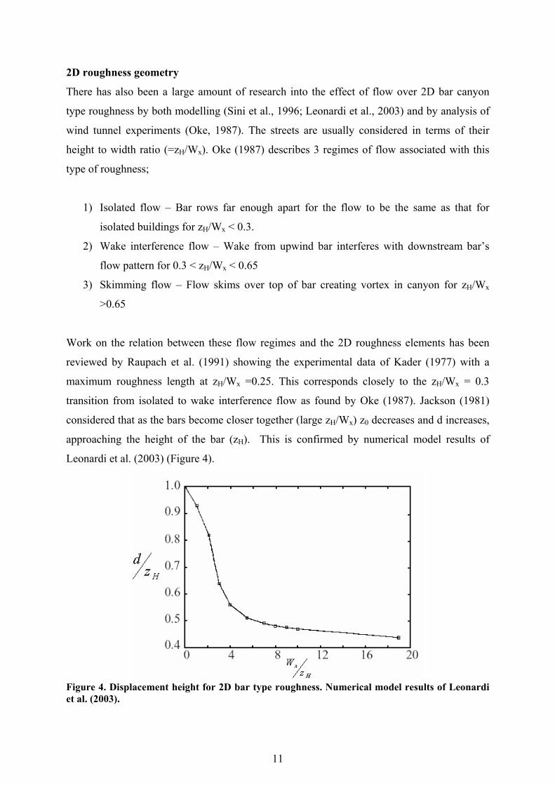
Work on the relation between these flow regimes and the 2D roughness elements has been
reviewed by Raupach et al. (1991) showing the experimental data of Kader (1977) with a
maximum roughness length at zH/Wx =0.25. This corresponds closely to the zH/Wx = 0.3
transition from isolated to wake interference flow as found by Oke (1987). Jackson (1981)
considered that as the bars become closer together (large zH/Wx) z0 decreases and d increases,
approaching the height of the bar (zH). This is confirmed by numerical model results of
Leonardi et al. (2003) (Figure 4).
Figure 4. Displacement height for 2D bar type roughness. Numerical model results of Leonardi et al. (2003).
12
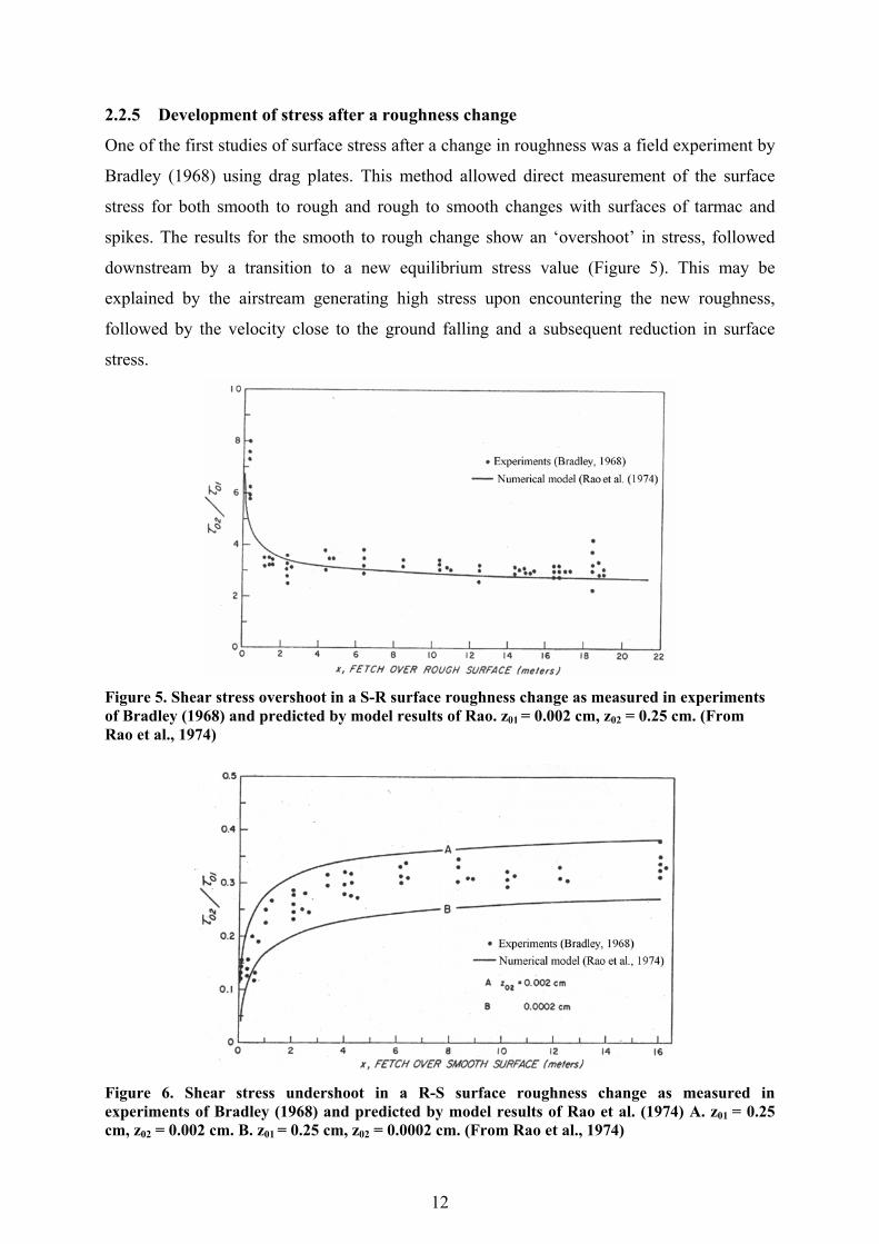
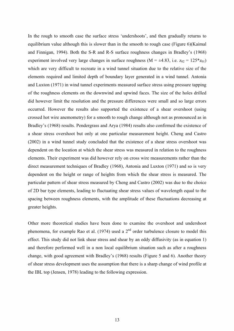
2.2.5 Development of stress after a roughness change
One of the first studies of surface stress after a change in roughness was a field experiment by
Bradley (1968) using drag plates. This method allowed direct measurement of the surface
stress for both smooth to rough and rough to smooth changes with surfaces of tarmac and
spikes. The results for the smooth to rough change show an ‘overshoot’ in stress, followed
downstream by a transition to a new equilibrium stress value (Figure 5). This may be
explained by the airstream generating high stress upon encountering the new roughness,
followed by the velocity close to the ground falling and a subsequent reduction in surface
stress.
Figure 5. Shear stress overshoot in a S-R surface roughness change as measured in experiments of Bradley (1968) and predicted by model results of Rao. z01 = 0.002 cm, z02 = 0.25 cm. (From Rao et al., 1974)
Figure 6. Shear stress undershoot in a R-S surface roughness change as measured in experiments of Bradley (1968) and predicted by model results of Rao et al. (1974) A. z01 = 0.25 cm, z02 = 0.002 cm. B. z01 = 0.25 cm, z02 = 0.0002 cm. (From Rao et al., 1974)
13
In the rough to smooth case the surface stress ‘undershoots’, and then gradually returns to
equilibrium value although this is slower than in the smooth to rough case (Figure 6)(Kaimal
and Finnigan, 1994). Both the S-R and R-S surface roughness changes in Bradley’s (1968)
experiment involved very large changes in surface roughness (M = ±4.83, i.e. z02 = 125*z01)
which are very difficult to recreate in a wind tunnel situation due to the relative size of the
elements required and limited depth of boundary layer generated in a wind tunnel. Antonia
and Luxton (1971) in wind tunnel experiments measured surface stress using pressure tapping
of the roughness elements on the downwind and upwind faces. The size of the holes drilled
did however limit the resolution and the pressure differences were small and so large errors
occurred. However the results also supported the existence of a shear overshoot (using
crossed hot wire anemometry) for a smooth to rough change although not as pronounced as in
Bradley’s (1968) results. Pendergrass and Arya (1984) results also confirmed the existence of
a shear stress overshoot but only at one particular measurement height. Cheng and Castro
(2002) in a wind tunnel study concluded that the existence of a shear stress overshoot was
dependent on the location at which the shear stress was measured in relation to the roughness
elements. Their experiment was did however rely on cross wire measurements rather than the
direct measurement techniques of Bradley (1968), Antonia and Luxton (1971) and so is very
dependent on the height or range of heights from which the shear stress is measured. The
particular pattern of shear stress measured by Cheng and Castro (2002) was due to the choice
of 2D bar type elements, leading to fluctuating shear stress values of wavelength equal to the
spacing between roughness elements, with the amplitude of these fluctuations decreasing at
greater heights.
Other more theoretical studies have been done to examine the overshoot and undershoot
phenomena, for example Rao et al. (1974) used a 2nd order turbulence closure to model this
effect. This study did not link shear stress and shear by an eddy diffusivity (as in equation 1)
and therefore performed well in a non local equilibrium situation such as after a roughness
change, with good agreement with Bradley’s (1968) results (Figure 5 and 6). Another theory
of shear stress development uses the assumption that there is a sharp change of wind profile at
the IBL top (Jensen, 1978) leading to the following expression.
14
2
02
1
2
ln1
⎥⎥⎥⎥
⎦
⎤
⎢⎢⎢⎢
⎣
⎡
⎟⎠⎞⎜
⎝⎛
−=
z
Miδτ
τ (16)
By consideration of the effect of displacement height Barlow (personal communication)
obtained:
( )( )( )( )
2
01
2
2
1
1
2 1ln
ln
⎥⎥⎥⎥⎥
⎦
⎤
⎢⎢⎢⎢⎢
⎣
⎡
+
⎟⎟⎠
⎞⎜⎜⎝
⎛ −
⎟⎟⎠
⎞⎜⎜⎝
⎛−−
=
zddd
i
i
i
δδδ
ττ (17)
It will not be possible to measure the IBL height accurately because the shear overshoot
occurs as the new roughness surface is encountered and the IBL depth is very small at this
point. Therefore δi is obtained from the theories of section 2.2.2 and so this shear stress ratio
is critically dependent on the accuracy of those theories.
2.3 Wind tunnel theory The use of a wind tunnel for this study is based on a need to simplify the complexity of real
life roughness changes in order to make the characteristic features of such a change more
identifiable. Also to properly ascertain what changes do occur is necessary to study the
boundary layer structure to a depth many times the height of the roughness elements. In a full
scale experiment this would very difficult as many very tall observation masts would be
needed at considerable effort and cost, and these would still not allow the measurements at the
many points that may be of interest to this study. Therefore a wind tunnel provides a
convenient platform for studying a change in surface roughness. However in order for the
results to be comparable to an atmospheric study the wind tunnel boundary layer should have
characteristics of a atmospheric boundary layer. The following guidelines (VDI, 2000) have
been considered;
2.3.1 Turbulence
A Wind tunnel boundary layer has to be turbulent, so the surface of the wind tunnel has to be
aerodynamically rough. Using the roughness Reynolds number (equation 18) smooth flow is
15
when Re* < 5 and fully rough flow is considered as Re* > 70 (Garratt, 1992; Raupach et al.,
1991). At high enough Reynolds number the structure of the turbulence in the inertial
sublayer is similar no matter what roughness type the surface is. Thus the turbulent features of
the atmospheric boundary layer obey this similarity in the wind tunnel providing the
roughness Reynolds number is large enough (> 5).
vzu 0*
*Re = (18)
Where ν - kinematic viscosity
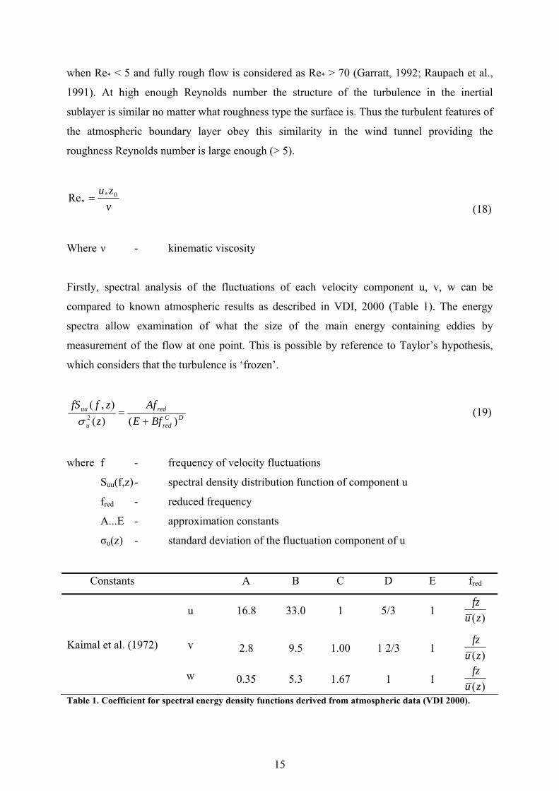
Firstly, spectral analysis of the fluctuations of each velocity component u, v, w can be
compared to known atmospheric results as described in VDI, 2000 (Table 1). The energy
spectra allow examination of what the size of the main energy containing eddies by
measurement of the flow at one point. This is possible by reference to Taylor’s hypothesis,
which considers that the turbulence is ‘frozen’.
DCred
red
u
uu
BfEAf
zzffS
)()(),(
2 +=
σ (19)
where f - frequency of velocity fluctuations
Suu(f,z) - spectral density distribution function of component u
fred - reduced frequency
A...E - approximation constants
σu(z) - standard deviation of the fluctuation component of u
Constants A B C D E fred
u 16.8 33.0 1 5/3 1 )(zufz
Kaimal et al. (1972) v 2.8 9.5 1.00 1 2/3 1 )(zufz
w 0.35 5.3 1.67 1 1 )(zufz
Table 1. Coefficient for spectral energy density functions derived from atmospheric data (VDI 2000).
16
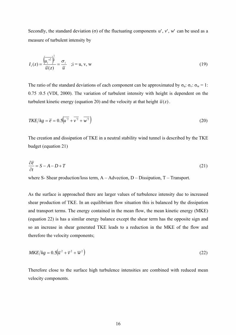
Secondly, the standard deviation (σ) of the fluctuating components ',',' wvu can be used as a
measure of turbulent intensity by
( )uzu
uzI ii
iσ
==)(
')(
21
2
;i = u, v, w (19)
The ratio of the standard deviations of each component can be approximated by σu: σv: σw = 1:
0.75 :0.5 (VDI, 2000). The variation of turbulent intensity with height is dependent on the
turbulent kinetic energy (equation 20) and the velocity at that height )(zu .
( )2'2'2'5.0 wvuekgTKE ++== (20)
The creation and dissipation of TKE in a neutral stability wind tunnel is described by the TKE
budget (equation 21)
TDASte
+−−=∂∂ (21)
where S- Shear production/loss term, A – Advection, D – Dissipation, T – Transport.
As the surface is approached there are larger values of turbulence intensity due to increased
shear production of TKE. In an equilibrium flow situation this is balanced by the dissipation
and transport terms. The energy contained in the mean flow, the mean kinetic energy (MKE)
(equation 22) is has a similar energy balance except the shear term has the opposite sign and
so an increase in shear generated TKE leads to a reduction in the MKE of the flow and
therefore the velocity components;
( )2225.0 wvukgMKE ++= (22)
Therefore close to the surface high turbulence intensities are combined with reduced mean
velocity components.
17
2.3.2 Wind profiles
Near the ground the log wind law can be used (equation 5). The profiles should be measured
at the upstream and downstream ends of the part of the wind tunnel under test for comparison
purposes. This is because the boundary layer produced in the wind tunnel should be in
equilibrium with the surface, that is, the velocity profiles, and turbulence characteristics
should not change significantly with fetch. Establishing an equilibrium part of the flow allows
changes brought about by the change in roughness to be resolved from changes that might
occur due to the changing nature of a non equilibrium flow.
2.3.3 Blockage
If elements of roughness are large then the flow may be excessively constricted by the tunnel
walls leading to increased pressure gradient and consequent acceleration of flow at the
blockage. A blockage coefficient is defined as
wt
proj
AA
=Φ (23)
where Aproj – projected area of obstacle along main wind direction.
Awt - wind tunnel cross-sectional area.
The limit set by VDI (2000) is Φ < 5% for enclosed measurement sections.

18
3 Wind tunnel setup The setup of the wind tunnel determines how the boundary layer is created in this study. The
appropriate use of the available apparatus and the individual limitations of each item of
equipment is what will limit the overall accuracy of the results obtained.
3.1 Apparatus
The wind tunnel comprises a working section 232x232x1500mm, with wind control provided
by a sucking fan operated via a transformer. Access is gained to the working section by
removable top sections, with one part having a 30cm long slot for hot wire entry. One pitot
tube for reference velocity measurements is located at (j), while another for use for hotwire
calibration is located at (k) (Figure 7).
To recreate the atmospheric boundary-layer in the wind tunnel with the limited fetch available
it is necessary to use an artificial method (Cook, 1978) rather than let one grow naturally.
Here this is in the form of spires in the arrangement shown in Figure 8. These initiate
turbulence producing a boundary layer of sufficient depth for experimentation. The roughness
elements work in conjunction with the spires, having the same role as in a naturally grown
boundary layer. They provide a drag on the wind such that a profile of Reynolds stress is
established which in turn controls the mean velocity profile and turbulence characteristics,
x
z y
a
b
c
d
e f
g hi
j k
Figure 7. Side view of wind tunnel setup. Dimensions of working section are 232x232x1500mm. a –hot wire probe height adjustment (Vernier scale), b – hot wire probe fetch adjustment and scale, c – hot wire probe, d – hot wire probe support, e – Lego™ roughness, f – street type roughness, g –air inflow, h – outlet fan, i –spires, j – pitot tube, k – reference pitot tube
19
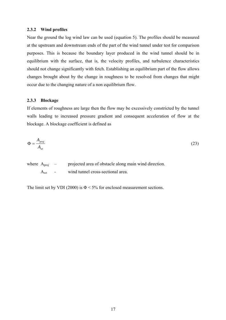
and thus u*, d and z0 (Cook, 1978).To check how well the wind and turbulence profiles
approximate the atmospheric boundary layer the criteria of the previous section were used.
3.1.1 Roughness element setup
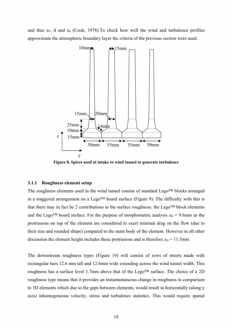
The roughness elements used in the wind tunnel consist of standard Lego™ blocks arranged
in a staggered arrangement on a Lego™ board surface (Figure 9). The difficulty with this is
that there may in fact be 2 contributions to the surface roughness: the Lego™ block elements
and the Lego™ board surface. For the purpose of morphometric analysis zH = 9.6mm as the
protrusions on top of the element are considered to exert minimal drag on the flow (due to
their size and rounded shape) compared to the main body of the element. However in all other
discussion the element height includes these protrusions and is therefore zH = 11.5mm.
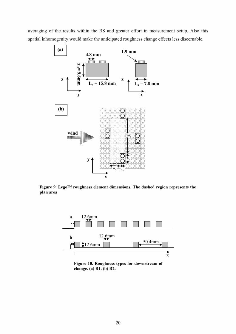
The downstream roughness types (Figure 10) will consist of rows of streets made with
rectangular bars 12.6 mm tall and 12.6mm wide extending across the wind tunnel width. This
roughness has a surface level 1.7mm above that of the Lego™ surface. The choice of a 2D
roughness type means that it provides an instantantaneous change in roughness in comparison
to 3D elements which due to the gaps between elements, would result in horizontally (along y
axis) inhomogeneous velocity, stress and turbulence statistics. This would require spatial
Figure 8. Spires used at intake to wind tunnel to generate turbulence
50mm 50mm55mm 55mm
10mm 15mm
25mm 14mm
15mm
10mm 15mm
20mm
z
y
20
averaging of the results within the RS and greater effort in measurement setup. Also this
spatial inhomogenity would make the anticipated roughness change effects less discernable.
Figure 9. Lego™ roughness element dimensions. The dashed region represents the plan area
yL
xL
yW
xW
wind
y
y
z
x
z Ly = 15.8 mm
zH = 9.6m
m
4.8 mm
Lx = 7.8 mm
1.9 mm
x
(a)
(b)
a
b
x
12.6mm
12.6mm
12.6mm
50.4mm
Figure 10. Roughness types for downstream of change. (a) R1. (b) R2.
21
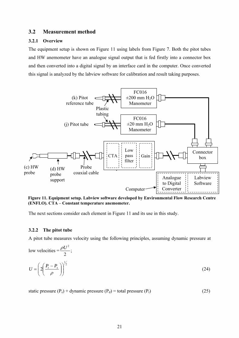
3.2 Measurement method 3.2.1 Overview
The equipment setup is shown on Figure 11 using labels from Figure 7. Both the pitot tubes
and HW anemometer have an analogue signal output that is fed firstly into a connector box
and then converted into a digital signal by an interface card in the computer. Once converted
this signal is analyzed by the labview software for calibration and result taking purposes.
The next sections consider each element in Figure 11 and its use in this study.
3.2.2 The pitot tube
A pitot tube measures velocity using the following principles, assuming dynamic pressure at
low velocities =2
2Uρ ;
21
2 ⎟⎟⎠
⎞⎜⎜⎝
⎛⎟⎟⎠
⎞⎜⎜⎝
⎛ −=
ρst PP
U (24)
static pressure (Ps) + dynamic pressure (Pd) = total pressure (Pt) (25)
CTALow pass filter
GainConnector
box
Analogue to Digital Converter
Labview Software
FC016 ±20 mm H2O Manometer
FC016 ±200 mm H2O
Manometer
(j) Pitot b
(k) Pitot reference tube
Plastic tubing
Hot wire (d) HW probe
Probe coaxial cable
Computer
Figure 11. Equipment setup. Labview software developed by Environmental Flow Research Centre (ENFLO). CTA – Constant temperature anemometer.
(j) Pitot tube
(c) HW probe
(d) HW probe support

22
Calibration of pitot tubes
The pressure transducer (manometer) measures the difference in pressure Pt-Ps=∆P and
displays this in mmH2O. To calibrate the pitot tube 8 point measurements are taken at
different tunnel speeds, with user inputted ∆P. The voltage output from the manometer has a
linear relationship to the mmH20 display, thus the Labview software calculates a best fit line
from the user inputted values and those from the voltage input. This best fit line describes the
response of the pitot tube allowing voltage to be converted into velocity with equation 24. The
pitot tube is not accurate at very low wind speeds so points are taken at wind tunnel speed
from 4 - 12ms-1. The sampling rate for these points is 1000Hz for a 20 second period. To try
and minimise turbulent fluctuations the spires are removed during calibration. The height of
each calibration is z = 178mm to avoid the influence of the surface and is kept the same in all
calibrations.
This procedure is repeated with the reference pitot tube and FC016 ±200mmH2O. This
manometer is not as accurate as the FC016 ±20mmH2O as it only uses a small part of its
range as it is meant for use at higher velocities.
3.2.3 The hot wire
The principle of hot wire anemometry is that airflow over a wire produces a cooling effect via
conduction into the air immediately surrounding it and subsequent convection and advection
of this air away from the wire. With constant temperature hot wire anemometry the
temperature of the wire is kept constant by a feedback differential amplifier, thus allowing
rapid variation of the heating current to compensate for instantaneous changes in the flow
velocity. A single normal tungsten hot wire is used which means that the hot wire is at 90
degrees to mean flow direction.
The main consideration in operation is that a high wire temperature gives high velocity
sensitivity but as the tungsten wire element of the hot wire oxidises at around 350oC the
temperature of the wire (Tw) must remain below this. (Bruun, 1995) The setting of the wire
temperature depends on the overheat ratio (a):
a=a
aw
RRR − (26)

23
where Rw - Resistance of heated wire at temperature (Tw)
Ra - Resistance of wire at ambient temperature (Ta)
When setting the overheat ratio the probe (Rp), probe prongs (Rp) and cable resistance (Rc)
must be taken into account;
cSpL RRRR ++=
where Rs – Resistances of connection leads in probe support
Rc – Resistance of probe cable
Rp – Resistance of probe (including prongs)
For this experiment the total lead resistance - RL is assumed to be 0.1Ω
Thus the total resistances are:
Laam RRR += (27a)
Lwwm RRR += (27b)
The temperature of the wire is given by:
20αaTT aw =− (28)
where α20 - Temperature coefficient of resistance at 20oC (~ambient temperature)
The single HW used in this experiment has aR =8.270 Ω, α20=0.36%K-1 and when operated at
an overheat ratio of 0.6 thus has Rw = 13.3 Ω and an operating temperature of 242oC.
Calibration
The output from the anemometer is first fed into an amplifier system with gain, low pass filter
settings and a zero-offset dial (see Figure 11). This allows the input voltage into the computer
interface card to be set within the input range, including the spikes and troughs of voltage
associated with a fluctuating turbulent flow. The low pass filter is set to half the required
frequency according to Nyquist criterion to avoid aliasing of high frequency components
(Kaimal and Finnigan, 1994). Therefore if sampling is at 3200Hz the low pass filter is set to
1600Hz. This voltage input is then calibrated against the pitot tube which is located at the
same height (169mm) and fetch (1245mm) and offset laterally 38.5mm.
24
The output voltage E = F(U) into the computer obeys King’s power law (Kaimal and
Finnigan, 1994)
nBUAE +=2 (29)
where A, B, n are coefficients determined by calibration and n ~ 0.45 but can use an optimal
value that gives the best goodness of fit or lowest normalised standard deviation εu.
3.2.4 The crossed hot wire
To obtain measurements of the covariance ''wu and therefore the shear stress it is necessary
to have simultaneous measurements of both u and w components within a small measurement
volume. A Dantec dynamics P61 crossed hot wire is used in this experiment.
The crossed hot wire has 2 wires perpendicular to each other. Each wire works independently
following the same principles to the single wire above. However when processing the
voltages from the 2 wires it is possible to break down the signal into its component parts u, v
or with 90 degree rotation of the hot wire, the u, w components. To do this it is necessary to
add an additional calibration procedure known as an angle calibration. Here calibration points
are taken at different incidences to the mean flow, e.g. from –25 to +25 degrees from the
mean flow vector. This calibration was only followed once during this experiment as the
angle between the wires should not change between each measurement day.
3.3 Measuring procedure Calibration of the pitot tubes and hot wire was nominally done once a day, as this calibration
can be adjusted by providing updated temperature and pressure measurements into the
Labview software at regular intervals (at the beginning of each profile in this experiment).
This correction is however only useful up to a change of 5oC from the calibration temperature
(Jørgensen, 2002). To ensure that the main energy containing range of turbulent spectra is
sampled measurements are taken at a sampling rate of 3200Hz with low pass filter at 1600Hz.
Different sampling periods were tested and a sampling period of 2 minutes was found to
allow second order statistics such as 2`u to reach a stable value and so was used throughout
the experiment.
25
Profile measurements were taken at logarithmic spacing of height z and where possible at the
same height intervals for each profile upwind and downwind of the roughness change. This
allows results at the same height to be compared with varying fetch. The hot wire is located in
a laterally central position (116mm from the tunnel sidewalls) and can be adjusted to any
fetch within the measurement section. Profile measurements were taken at varying fetches.
Due to the staggered nature of the roughness elements this allows a spatial average of the
profile parameters within the RS (Appendix 1). This should also reveal if there are any
variation of profiles with fetch x. Due to the size of the probe it was not possible to measure
profiles in the canopy layer directly in front of a Lego™ element and profiles behind Lego™
elements sometimes required the removal of a Lego™ element downstream to facilitate
access to canopy layer element height velocity measurements. As well as the upstream
profiles, additional profiles were taken at fetches greater than x = 1032mm where the new
roughness was to be located for comparison purposes with the profiles obtained when it is in
place.
3.4 Sources of error Overall error is typically 3% for velocity measurements. The most important contributions to
this are from the calibration, linearization and temperature errors. These are described in the
following sections.
3.4.1 Temperature
This is usually the most important source of error, of approximately 2% in wind velocity 1o
change in temperature for a wire operated at overheat ratio of 0.8. This can be accounted for
after calibration although temperature measurements need to be taken regularly. For example
in the morning when the room’s temperature may be varying rapidly one profile of 16
samples each of 2 minutes duration will take approximately 45 minutes, which is enough time
for a large temperature rise (~1oC) and error to occur.
3.4.2 Calibration error
The error due to calibration is due to the error associated with the pitot tube pressure
measurement. A resolution of 0.01 mmH20 corresponds to an error of 0.1% at the operating
speed of this experiment (~8ms-1). This error would however be significant at lower
velocities. There are also curve fitting errors (linearization errors) which occur during
calibration and are usually measured in terms of normalised standard deviation εu. For the
26
single wire the average curve fitting error of all calibrations was εu=0.22%, and for the cross
wires ε = 0.l3% and εu =0.2 % for pitot tube calibrations.
3.4.3 Pressure variations
It is important to re-zero the manometers after each profile otherwise the velocity
measurements will be subject to a gradual drift during a day’s experimentation. Also
calculation by the software of the hot wire velocity is also sensitive to pressure variations due
to changes in density that affect the mass transfer (ρU), and therefore heat transfer over the
hot wire. The pressure variation error is typically 0.6 % for the pressure fluctuations
experienced during one day’s experiment. This effect is however minimised due to the
inputting of ambient pressure into the Labview software before each profile during
measurements.
3.4.4 Probe positioning
As long as the hot wire is kept in the same position as during calibration and measurement
this error is likely to be negligible. If however there is misalignment with the pitot tube during
calibration then a systematic error will be present in that day’s results. However this should
only be small as the eye is estimated be able to judge perpendicular angles ±2o, or
equivalently as uθ varies as u(1-cos θ), a 0.5% error at standard tunnel free stream operating
speed (8ms-1) (Jørgensen, 2002).
3.4.5 High turbulence intensity errors
Cross wire anemometers are subject to additional errors may occur when the velocity is
incident on the hot wire at an angle outside the acceptable range. Also there are effects due to
sheltering of the flow to one wire by the other wire in high turbulence intensities. This
generally becomes significant at turbulent intensities over 0.2. The effect causes a cross wire
to overestimate the mean wind speed and underestimate the Reynolds stress (Tutu and
Chevray, 1975). For example a turbulence intensity of 0.3 then the shear stress is
underestimated by approximately 25%, and the mean velocity overestimated by 7% (Tutu and
Chevray, 1975). Error estimates for other turbulent intensities are given in Appendix 5. These
errors could be corrected for but their calculation for all the results is beyond the scope of this
project.
27
4 Results and analysis The results of profile measurements at different fetches over two different roughness changes
R1 and R2 are presented here. Firstly the upwind (Lego™) and both downwind (R1 and R2)
surfaces z0 and d values are calculated using morphometric analysis to allow comparison with
those obtained by measurements. The upwind surface velocity and shear stress and turbulence
properties are discussed, followed by the corresponding results with increasing fetch after the
roughness changes to both R1 and R2. The IBL height and shear stress ratios are then
calculated and compared to various theories.
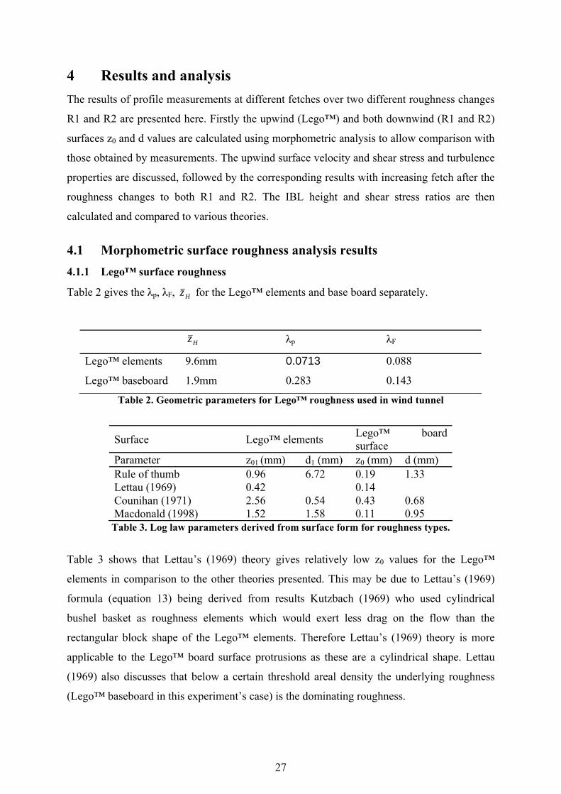
4.1 Morphometric surface roughness analysis results 4.1.1 Lego™ surface roughness
Table 2 gives the λp, λF, Hz for the Lego™ elements and base board separately.
Table 2. Geometric parameters for Lego™ roughness used in wind tunnel
Surface Lego™ elements Lego™ board surface
Parameter z01 (mm) d1 (mm) z0 (mm) d (mm) Rule of thumb 0.96 6.72 0.19 1.33 Lettau (1969) 0.42 0.14 Counihan (1971) 2.56 0.54 0.43 0.68 Macdonald (1998) 1.52 1.58 0.11 0.95
Table 3. Log law parameters derived from surface form for roughness types.
Table 3 shows that Lettau’s (1969) theory gives relatively low z0 values for the Lego™
elements in comparison to the other theories presented. This may be due to Lettau’s (1969)
formula (equation 13) being derived from results Kutzbach (1969) who used cylindrical
bushel basket as roughness elements which would exert less drag on the flow than the
rectangular block shape of the Lego™ elements. Therefore Lettau’s (1969) theory is more
applicable to the Lego™ board surface protrusions as these are a cylindrical shape. Lettau
(1969) also discusses that below a certain threshold areal density the underlying roughness
(Lego™ baseboard in this experiment’s case) is the dominating roughness.
Hz λp λF
Lego™ elements 9.6mm 0.0713 0.088
Lego™ baseboard 1.9mm 0.283 0.143
28
Counihan’s (1971) equations describe the results obtained in wind tunnel experiments using
Lego™ elements on a Lego™ base board and so has specific application to the current
experiment. However the λp values for the Lego™ elements for this experiment are outside
the limits chosen by Counihan (1971) of 25.01.0 << pλ for equation 14a so Grimmond and
Ork’s (1999) curve fit of Counihan’s (1971) results is used (equation 14c).
The coefficients used for Macdonald et al. (1998) are, CD = 1.2 for standard 2x1 Lego™
block, β =1.32 for Lego™ elements and β =0.8 for Lego™ board protrusions. These are
calculated (ESDU, 1989) with expected turbulent intensities, velocity profiles and length
scales as found in previous experiments on this surface in this wind tunnel (Pascheke,
personal communication).
The ‘rule of thumb’, Counihan (1971) and Macdonald et al. (1998) results do not show good
agreement for the Lego™ elements z0 (0.96mm< z01 <2.56mm) or d1 (0.54mm < d1 <
1.58mm). In the case of Counihan (1971) the low λp, λF values for the Lego™ elements are
outside the experimental results from which Counihan’s (1971) equation is based on. The
‘rule of thumb’ is based on height alone, does not consider the densities λp, λF and has
coefficients based on mean values for land surfaces. Thus as such a low λp, λF values are not
typical of most surfaces (Grimmond and Oke, 1999) the ‘rule of thumb’ method is considered
to provide an overestimate of d. Macdonald et al. (1998) theory is considered the most
applicable to this Lego™ element surface as it is derived from fundamental principles and has
correction factors for the many different aspects that could affect z0 and d such as velocity
profile, turbulence and rounded edges. However because the wind tunnel elements work in
conjunction with the spires at the start of the wind tunnel the values of z01 and d1 are
somewhat influenced by the spire setup which cannot be accounted for in these methods.
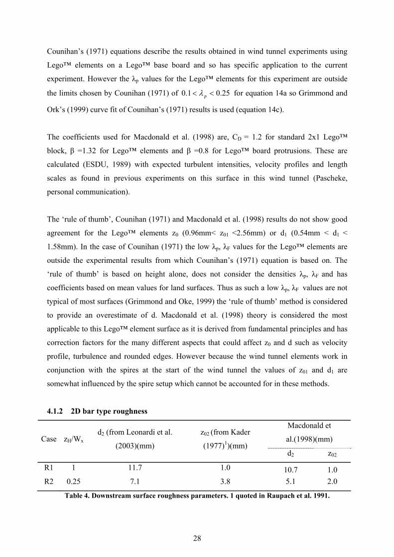
4.1.2 2D bar type roughness
Macdonald et
al.(1998)(mm) Case zH/Wx d2 (from Leonardi et al.
(2003)(mm)
z02 (from Kader
(1977)1)(mm) d2 z02
R1 1 11.7 1.0 10.7 1.0 R2 0.25 7.1 3.8 5.1 2.0
Table 4. Downstream surface roughness parameters. 1 quoted in Raupach et al. 1991.

29
There is excellent agreement between the above theories for R1, but for R2 there are slightly
smaller values of z02 and d2 predicted by Macdonald et al. (1998) compared to Leonardi et al.
(2003) and Kader (1977). It is also noted that due to the small cross sectional area of the wind
tunnel the blockage factor (Φ) for these element sizes is 6.9%, which is over the 5% VDI
guideline. Streamwise velocity measurements are made to test what effect this has on
windspeed at a reference height.
Using Macdonald et al. (1998) theory the change of surface roughness from Lego™ to R1
should have the effect of a modest decrease in surface roughness (with M =-0.42 (rough to
smooth)) but large increase of displacement height (d2 = 6.8d1). In comparison the change of
surface roughness from Lego™ to R2 should result in an increase in roughness length
(M=0.69 (smooth to rough)) and smaller increase in displacement height (d2 = 3.2d1).
4.2 Profiles above upstream Lego™ roughness 4.2.1 Introduction
The location of profile measurements over the Lego™ surface roughness are shown in
Appendix 1. The results of these measurements are shown in Figure 12. Many profiles were
taken but due to large changes in temperature (∆T > +1oC) during some measurements there
were errors that were considered too large (>5%) to allow a good comparison with other
profiles and so these were not included, but are displayed in Appendix 2.

30
(a)
z (m
m)
0.750.500.250.00
100
1011.5
23
34.5
Variablex = 955 mmx = 1051 mmx = 1128 mmx = 1202 mm
(b) u component Turbulent Intensity0.50.40.30.20.10.0
100
10
2Zh
Zh
3Zh
Figure 12. (a) Normalised wind profiles over Lego™ surface (b) u component turbulent intensity profiles over Lego™ surface. Measured with single HW. The normalised wind velocity u/upref at reference height z = 178mm would be expected to be
close to 1 as this is the height of the pitot tube. However this does not occur in this experiment
(Figure 12). This may be due to a number of reasons, for example the reference pitot tube is
located downwind and at a different y location relative to the hot wire and so any pressure
gradient in the wind tunnel may have a consistent effect of relatively low hot wire velocities.
There may also be horizontal variations (in y) that were not tested due to difficulties in
equipment arrangement. Differing alignments of pitot tube, calibrating pitot tube or hot wire
could cause lower velocities to be recorded as any flow approach angle other than
perpendicular to the tube would result in a lower windspeed as shown in section 3.4.4. The
lower velocity compared to the reference tube is a consistent feature of every profile taken
during the experiment and it is unlikely that alignment is the main cause of these errors. The
lower velocities recorded do not affect the conclusions of this experiment as long as there is
not large velocity variation with fetch at the reference height over the test section. This was
tested (Appendix 3) and found to be a variation of 1.5% which is within the error bounds for
velocity measurements (3%) and so not significant.
prefuu /
Hz
Hz2Hz3
31
(a) -u'w'/Upref^2
z (m
m)
0.0040.0030.0020.0010.000
200
150
100
50
0Zh2Zh3Zh3Zh2ZhZh
(b) -u'w'/u*^2
z (m
m)
1.51.00.50.0-0.5
200
150
100
50
0Zh2Zh3Zh
Variablex = 920 mmx = 946 mm
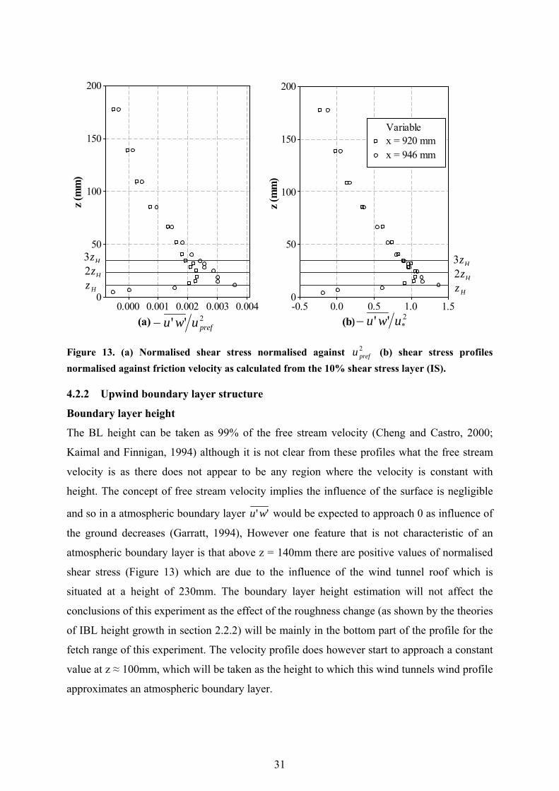
Figure 13. (a) Normalised shear stress normalised against 2prefu (b) shear stress profiles
normalised against friction velocity as calculated from the 10% shear stress layer (IS). 4.2.2 Upwind boundary layer structure
Boundary layer height
The BL height can be taken as 99% of the free stream velocity (Cheng and Castro, 2000;
Kaimal and Finnigan, 1994) although it is not clear from these profiles what the free stream
velocity is as there does not appear to be any region where the velocity is constant with
height. The concept of free stream velocity implies the influence of the surface is negligible
and so in a atmospheric boundary layer ''wu would be expected to approach 0 as influence of
the ground decreases (Garratt, 1994), However one feature that is not characteristic of an
atmospheric boundary layer is that above z = 140mm there are positive values of normalised
shear stress (Figure 13) which are due to the influence of the wind tunnel roof which is
situated at a height of 230mm. The boundary layer height estimation will not affect the
conclusions of this experiment as the effect of the roughness change (as shown by the theories
of IBL height growth in section 2.2.2) will be mainly in the bottom part of the profile for the
fetch range of this experiment. The velocity profile does however start to approach a constant
value at z ≈ 100mm, which will be taken as the height to which this wind tunnels wind profile
approximates an atmospheric boundary layer.
Hz3Hz2
Hz
Hz3Hz2
Hz
2'' prefuwu− 2*'' uwu−

32
Roughness sublayer
The roughness sublayer (RS) can be considered as the region influenced directly by the
elements (Garratt, 1994). Over this Lego™ surface the profiles of velocity (Figure 12a),
turbulent intensity (Figure 12b) and normalised shear stress (Figure 13b) vary significantly
with fetch x around an element up until approximately 2zH, which is taken as the RS top.
Within the canopy layer there is a large variation of velocity and turbulent intensity (Figure
12). This spatial inhomogenity is due to the changing location of the HW probe in relation to
the elements and consequent measurements of different parts of the wake flow from the
roughness elements as found by (Raupach et al., 1980). For example the x = 1202 mm profile
is directly behind an element and so has almost constant velocity until above zH due to
sheltering, then above this there is strong wind shear and therefore strong shear production of
TKE and a resulting high turbulence intensity (equation 20,21) in the wake flow immediately
behind the element (turbulent intensity = 0.52 for x = 1202mm at z = 12mm, Figure 12b) as
found by Roth (2000). The greater the fetch after the upstream roughness element the greater
the average velocity in the canopy layer and the lower the average turbulent intensity. This is
due to less wind shear and corresponding lower turbulent intensity. The shear stress decreases
at the top of the canopy layer (zH) due to the influence of the surface. This is supported by the
results of Raupach et al. (1980), Antonia and Luxton (1971). Normalisation of the stress
profiles against u* shows that the data collapses into one line, with a shape in good agreement
with Raupach et al. (1980) and Pendergrass and Arya (1984) although the latter experiment in
particular has a much deeper constant flux (~10 % stress) layer. This may be due to the much
larger wind tunnel and subsequent larger upwind fetch (8m) to allow this layer to develop.
The Inertial sublayer
The inertial sublayer is conventionally taken as the region of constant stress to within 10%
(Oke, 1987). Above the RS a 10 % variation extends from 23mm to 32mm ((~2-3)zH as found
by Raupach et al. (1991) in a review of laboratory and field experiments) in both the shear
stress profiles taken. It is also noted that velocity and turbulence intensity profiles show the
most consistency with fetch in the 2zH to 3zH height range in agreement with the assumptions
of horizontal homogeneity implicit in the log law derivation (section 2.1). u* (IS) values taken
from averaging the shear stress measurements within this range are calculated (Table 5) and
used to fit a log law and thus derive z0 and d. One consideration is that this constant stress
layer is not very deep and only 3 measurements per profile were taken in this region. This
shallowness could be due to the way in which the BL was formed artificially with insufficient
33
fetch to allow this layer to deepen. However this may be appropriate to a real boundary layer
as there is rarely enough fetch for an equilibrium layer to form due to the heterogeneity of real
surfaces. As stated by Roth (2000) in urban areas very little is known about the IS as it is
often out of the range of meteorological measurement towers and due to the often large
vertical extent of the RS may be very small if it exists at all. For comparison the velocity
profiles are fitted for this range using an iterative process (in Curvexpert software) to give
values of z0, u* and d independently of the shear stress measurements.
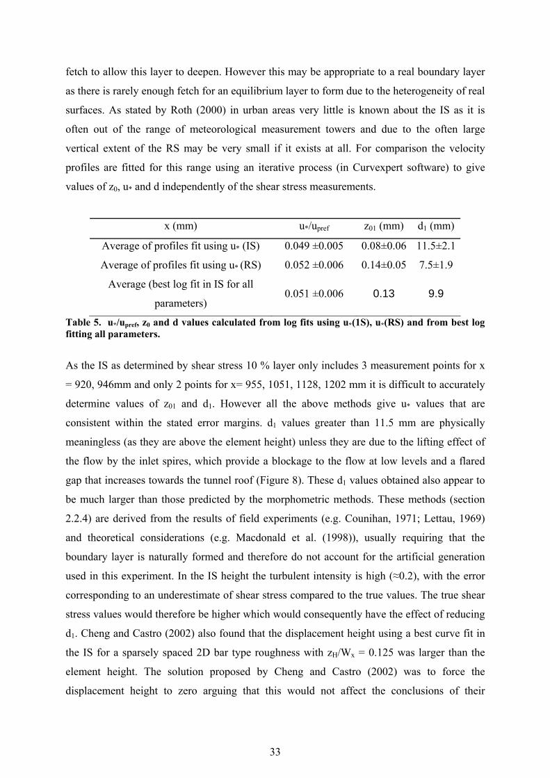
x (mm) u*/upref z01 (mm) d1 (mm)
Average of profiles fit using u* (IS) 0.049 ±0.005 0.08±0.06 11.5±2.1
Average of profiles fit using u* (RS) 0.052 ±0.006 0.14±0.05 7.5±1.9
Average (best log fit in IS for all
parameters) 0.051 ±0.006 0.13 9.9
Table 5. u*/upref, z0 and d values calculated from log fits using u*(1S), u*(RS) and from best log fitting all parameters.
As the IS as determined by shear stress 10 % layer only includes 3 measurement points for x
= 920, 946mm and only 2 points for x= 955, 1051, 1128, 1202 mm it is difficult to accurately
determine values of z01 and d1. However all the above methods give u* values that are
consistent within the stated error margins. d1 values greater than 11.5 mm are physically
meaningless (as they are above the element height) unless they are due to the lifting effect of
the flow by the inlet spires, which provide a blockage to the flow at low levels and a flared
gap that increases towards the tunnel roof (Figure 8). These d1 values obtained also appear to
be much larger than those predicted by the morphometric methods. These methods (section
2.2.4) are derived from the results of field experiments (e.g. Counihan, 1971; Lettau, 1969)
and theoretical considerations (e.g. Macdonald et al. (1998)), usually requiring that the
boundary layer is naturally formed and therefore do not account for the artificial generation
used in this experiment. In the IS height the turbulent intensity is high (≈0.2), with the error
corresponding to an underestimate of shear stress compared to the true values. The true shear
stress values would therefore be higher which would consequently have the effect of reducing
d1. Cheng and Castro (2002) also found that the displacement height using a best curve fit in
the IS for a sparsely spaced 2D bar type roughness with zH/Wx = 0.125 was larger than the
element height. The solution proposed by Cheng and Castro (2002) was to force the
displacement height to zero arguing that this would not affect the conclusions of their

34
experiment. The fit of u*(IS) and the corresponding z01 and d1 values is shown in comparison
with the average wind profile in Appendix 4.
The Roughness Reynolds number (equation 18) of this flow using u*(IS) and corresponding
log fit value of z0 is Re* = 2.3 corresponding to a non turbulent flow as described by Raupach
et al, 1991. However as stated above d1 is unrealistically large, leading to a small z0 value. In
contrast when the value of z0 calculated using the morphometric method of Macdonald et al.
(1998) is used the Reynolds number is Re* = 43.3 which corresponds to turbulent flow
(Raupach et al. 1991)
An average of ''wu over the RS (not including the canopy layer) was also used to calculate
u*(RS) (as in Cheng and Castro, 2002) (Table 5), although there is a lack of sufficient profiles
to obtain a good spatial average. However u*(RS) values taken from ''wu measurements in
the RS are not representative as the turbulence within this layer is distinctly organised due to
the influence of the element geometry, and part of momentum flux is non turbulent (Wieringa,
1993). Also as the wind flow is horizontally inhomogeneous within this region, so
representative u* values will be difficult to obtain except by extensive measurements in order
to obtain a good spatial average. However in field measurements it is most likely that profile
measurements are being taken in the RS and this is more likely over very rough urban surface
where the IS is usually out of the height range of all but the tallest masts and may not even
exist at all over such heterogeneous surfaces.
Reference δ/z01 u*(IS)/upref
Pendergrass and Arya (1984) 3D array of blocks 1150 0.054
Cheng and Castro (2002) 104 0.070
Counihan (1975)1 500-1500 0.043-0.06
Present experiment 1000±300 0.049
Table 6. Comparison table of u* (IS)/upref values. 1. A review of urban atmospheric data
Table 6 gives a summary of the u*(IS)/upref results found by different authors. Cheng and
Castro (2002) have a particularly small ratio δ/z01 which is due to the forcing of d1 to zero
which may result in a particularly large z01 value if a significant non-zero displacement height
does exist for their surface. Other authors find similar values (within ± 0.005 error limits) of
u*(IS)/ upref although no indication is given of the uncertainty of these measurements, which
35
may be considerable (>10%) for measurements of ''wu in the IS. Counihan’s (1975) review
also indicates that the current study has values typical of urban areas. The concern of the use
of upref as a normalising factor for comparisons is that this pitot tube is located downstream of
the hot wire and pressure differences may cause the wind tunnel speed to increase towards the
back of the wind tunnel, leading to the normalised velocity at reference height not reaching
unity as shown in Figure 12a.
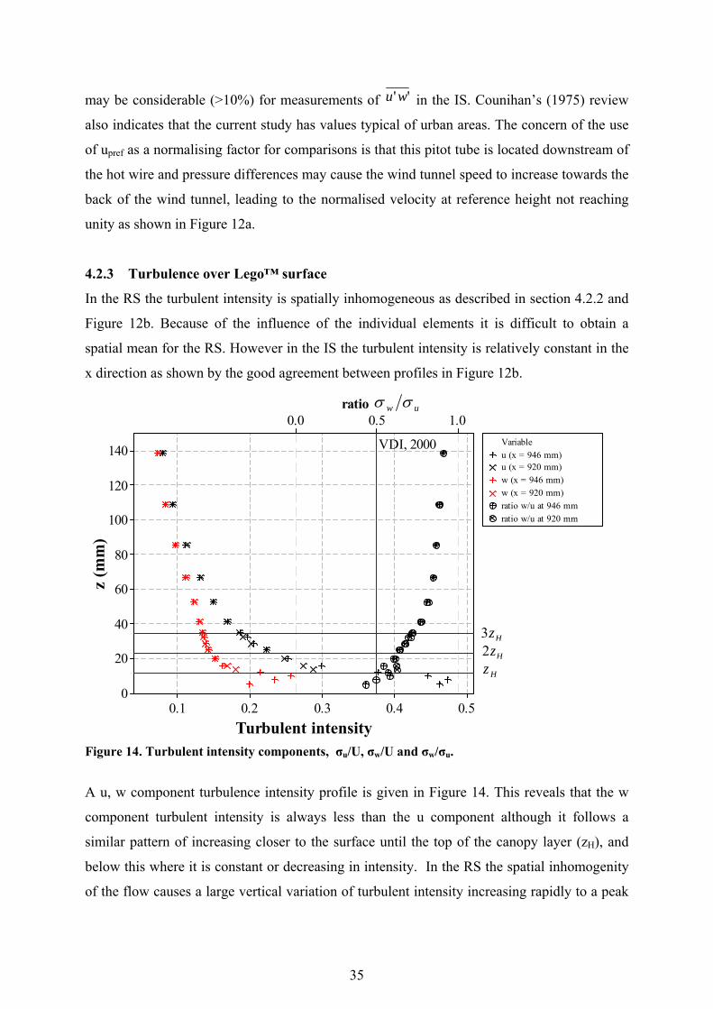
4.2.3 Turbulence over Lego™ surface
In the RS the turbulent intensity is spatially inhomogeneous as described in section 4.2.2 and
Figure 12b. Because of the influence of the individual elements it is difficult to obtain a
spatial mean for the RS. However in the IS the turbulent intensity is relatively constant in the
x direction as shown by the good agreement between profiles in Figure 12b.
Turbulent intensity
ratio TIw/TIu
z (m
m)
0.50.40.30.20.1
140
120
100
80
60
40
20
0
1.00.50.0
VDI, 2000
Zh2Zh3Zh
Variable
ratio w/u at 946 mmratio w/u at 920 mm
u (x = 946 mm)u (x = 920 mm)w (x = 946 mm)w (x = 920 mm)
Figure 14. Turbulent intensity components, σu/U, σw/U and σw/σu.
A u, w component turbulence intensity profile is given in Figure 14. This reveals that the w
component turbulent intensity is always less than the u component although it follows a
similar pattern of increasing closer to the surface until the top of the canopy layer (zH), and
below this where it is constant or decreasing in intensity. In the RS the spatial inhomogenity
of the flow causes a large vertical variation of turbulent intensity increasing rapidly to a peak
uw σσ
Hz3Hz2
Hz

36
at zH followed by a decrease towards the surface. However more profiles would have to be
taken to get a good picture of the spatial distribution of turbulent intensity in the RS. This is
evident by the large difference in σw/σu ratios in this layer as opposed to the good agreement
of these in the IS and above. The ratio of σw/σu is larger than the VDI (2000) guideline except
for the 946mm case at less than the element height zH = 11.5 mm = 23m. Because these ratios
are approximate and are derived from field experiments that only have a limited height (z = 0
– 50m) range they are only appropriate for heights close to the ground. As the height from the
surface increases it would be expected that due to the decreasing influence of the ground
surface the turbulent intensity components would approach a 1:1:1 ratio. There is relatively
small vertical variation in the ratios of each turbulent intensity component within the region
11.5-19 mm as found by Roth (2000) in his review of turbulence over cities. It must be noted
that the turbulence values for the u component are <30 % and are subject to additional errors
as described in the section 3.4.5 and Appendix 5.
Turbulent intensity
z (m
m)
0.50.40.30.20.1
140
120
100
80
60
40
20
0
1.11.00.50.0 VDI, 2000
Zh2Zh3Zh
Variable
Ratio v/u (991 mm)Ratio v/u (955 mm)
u (x = 991 mm)u (x = 955 mm)v (x= 991 mm)v (x = 955 mm)
(b)
Figure 15. Turbulent intensity components, σu/U, σv/U and σv/σu.
Figure 15 shows that the ratio of v to u components is in the correct range within 1 - 1.5zH
(equivalently 23m - 32m in full scale), which is the correct range when compared to
atmospheric measurements. Above 85.2mm this ratio becomes consistently greater than 1
which is not a feature of atmospheric turbulence. This effect is probably due to the way
Hz3Hz2
Hz
uv σσ
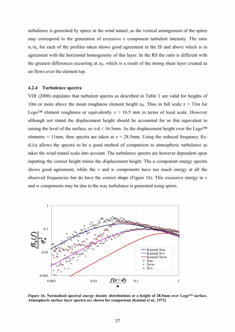
37
turbulence is generated by spires in the wind tunnel, as the vertical arrangement of the spires
may correspond to the generation of excessive v component turbulent intensity. The ratio
σv/σu for each of the profiles taken shows good agreement in the IS and above which is in
agreement with the horizontal homogeneity of this layer. In the RS the ratio is different with
the greatest differences occurring at zH, which is a result of the strong shear layer created as
air flows over the element top.
4.2.4 Turbulence spectra
VDI (2000) stipulates that turbulent spectra as described in Table 1 are valid for heights of
10m or more above the mean roughness element height zH. Thus in full scale z > 33m for
Lego™ element roughness or equivalently z > 16.5 mm in terms of local scale. However
although not stated the displacement height should be accounted for as this equivalent to
raising the level of the surface, so z-d < 16.5mm. As the displacement height over the Lego™
elements ≈ 11mm, then spectra are taken at z = 28.5mm. Using the reduced frequency f(z-
d1)/u allows the spectra to be a good method of comparison to atmospheric turbulence as
takes the wind tunnel scale into account. The turbulence spectra are however dependent upon
inputting the correct height minus the displacement height. The u component energy spectra
shows good agreement, while the v and w components have too much energy at all the
observed frequencies but do have the correct shape (Figure 16). This excessive energy in v
and w components may be due to the way turbulence is generated using spires.
0.001
0.01
0.1
1
0.001 0.01 0.1 1
Kaimal SuuKaimal SvvKaimal SwwSuu Sww Svv
Figure 16. Normalised spectral energy density distributions at a height of 28.5mm over Lego™ surface. Atmospheric surface layer spectra are shown for comparison (Kaimal et al., 1972)

38
4.3 Profiles over R1 roughness type Normalised wind profiles show differences between different fetches (Figure 17), e.g. at the
reference height (z=178mm) these differences are large (~5%) but show no pattern with fetch.
Therefore these differences are most likely due to errors incurred during measurement or
calibration. In comparison to the Lego™ profiles, where profiles were rejected if the
temperature changed significantly during a profile, the constraints of time and the occurrence
of exceptionally hot weather during the measurement days over R1 meant that large
temperature changes (+1oC) did occur. Because the main points of interest were considered to
lie in the bottom part of the profile to minimise error the profiles were taken from the bottom
upwards and therefore shortly after a calibration correction temperature reading. However a
1oC change should only contribute a 2% error and so additional factors must have been
influencing the readings. These could include the blockage factor (Φ) increase of 6.25%,
causing an acceleration of flow speed due to the decrease in cross-sectional area over the bar
roughness. This was assessed by a measuring windspeed at the reference height of z = 178mm
and was determined to be 2.5% speed increase over the x = 1032 - 1190mm fetch (Appendix
3). There may also be additional errors from calibration and due to hot wire and two pitot
tubes alignment changing in-between profiles.
Uhw/Upref
z (m
m)
1.00.90.80.70.60.50.4
160
100
80
60
40
20
10
Zh
2Zh
3Zh
Variable
z (mm) * (x=1077mm) Uhw/Uprefz (mm) * (x=1089mm) Uhw/Uprefz (mm) * (x=1102mm) Uhw/Uprefz (mm) * (x=1115mm) Uhw/Uprefz (mm) * (x=1127.5mm) Uhw/Uprefz (mm) * (x=1140mm) Uhw/Uprefz (mm) * (x=1153mm) Uhw/Uprefz (mm) * (x=1166mm) Uhw/Uprefz (mm) * (x=1178mm) Uhw/Uprefz (mm) * (x=1190mm) Uhw/Upref
C16 * Upwind legoz (mm) * (x=1038mm) Uhw/Uprefz (mm) * (x=1051mm) Uhw/Uprefz (mm) * (x=1064mm) Uhw/Upref
Figure 17. Wind profiles after change in roughness from Lego™ to R1 type roughness including upwind velocity profile for comparison.
prefuu /
Hz3
Hz2
Hz

39
4.3.1 Initial flow disturbance
Features within the bottom of the profile include the relatively high velocities in the range z =
18.2 – 32mm over first bar roughness (x = 1038mm) compared to the upstream profile (Figure
17). The estimation of the lower limit of this acceleration is set by the lowest measurement
possible and the upper limit is the height of re-mergence with the upstream profile although
this is only approximate due to the large scatter of data. The basic elements of this flow
feature are shown in Figure 18.
The acceleration of the flow over bar 1 is due to streamlines converging, creating a jet as
shown in Figure 18. This feature is supported by the positive values of normalised shear stress
(Figure 19) at this point, showing that the locally the momentum of the wind at 18.2mm is not
acting upwards rather than downwards on the surface as the airflow is forced up over the bar
by the pressure increase on the bar’s upstream face. Because of this upward motion the shear
stress is positive and therefore TKE decreases compared to upstream values due the shear
production becoming locally very small/ negative. However although the results indicates
shear stress loss it is unlikely as this signifies a counter gradient flux. This may be due to the
error associated with the velocity gradient term at this point.
Compared to the upwind Lego™ profile, after the initial faster flow over the first bar and
canyon, profiles at greater fetches (i.e. after bar 2) show slower velocities up to a height of z =
36mm. The scatter of data does however make it difficult to draw any conclusions about if
Displacement zone
CavityCavity
Wake
zH
3zH
Figure 18. Flow disturbance caused by roughness change (adapted from Oke, 1987).
1 2
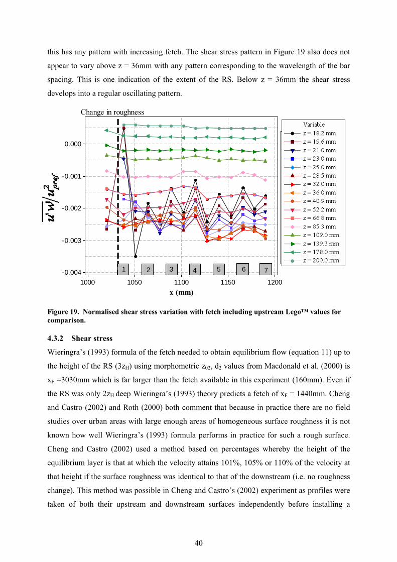
40
this has any pattern with increasing fetch. The shear stress pattern in Figure 19 also does not
appear to vary above z = 36mm with any pattern corresponding to the wavelength of the bar
spacing. This is one indication of the extent of the RS. Below z = 36mm the shear stress
develops into a regular oscillating pattern.
x (mm)
u'w
'/Upr
ef2
12001150110010501000
0.000
-0.001
-0.002
-0.003
-0.004
Change in roughness
Variable
z = 21.0 mmz = 23.0 mmz = 25.0 mmz = 28.5 mmz = 32.0 mmz = 36.0 mmz = 40.9 mmz = 52.2 mmz = 66.8 mmz = 66.8 mm
z = 18.2 mm
z = 85.3 mmz = 109.0 mmz = 139.3 mmz = 178.0 mmz = 200.0 mm
z = 19.6 mm
1 2 3 4 5 6 7
Figure 19. Normalised shear stress variation with fetch including upstream Lego™ values for comparison. 4.3.2 Shear stress
Wieringra’s (1993) formula of the fetch needed to obtain equilibrium flow (equation 11) up to
the height of the RS (3zH) using morphometric z02, d2 values from Macdonald et al. (2000) is
xF =3030mm which is far larger than the fetch available in this experiment (160mm). Even if
the RS was only 2zH deep Wieringra’s (1993) theory predicts a fetch of xF = 1440mm. Cheng
and Castro (2002) and Roth (2000) both comment that because in practice there are no field
studies over urban areas with large enough areas of homogeneous surface roughness it is not
known how well Wieringra’s (1993) formula performs in practice for such a rough surface.
Cheng and Castro (2002) used a method based on percentages whereby the height of the
equilibrium layer is that at which the velocity attains 101%, 105% or 110% of the velocity at
that height if the surface roughness was identical to that of the downstream (i.e. no roughness
change). This method was possible in Cheng and Castro’s (2002) experiment as profiles were
taken of both their upstream and downstream surfaces independently before installing a
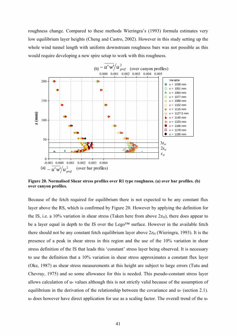
41
roughness change. Compared to these methods Wieringra’s (1993) formula estimates very
low equilibrium layer heights (Cheng and Castro, 2002). However in this study setting up the
whole wind tunnel length with uniform downstream roughness bars was not possible as this
would require developing a new spire setup to work with this roughness.
-u'w'/Upref 2
-u'w'/Upref 2
z (m
m)
0.0040.0030.0020.0010.000-0.001
200
150
100
50
0
0.0050.0040.0030.0020.0010.000
Zh2Zh3Zh
Variable
x = 1089 mmx = 1102 mmx = 1115 mmx = 1127.5 mmx = 1140 mmx = 1153 mmx = 1166 mmx = 1178 mmx = 1190 mm
x = 1038 mmx = 1051 mmx = 1064 mmx = 1077 mm
(over canyon profiles)
(a)
(b)
(over bar profiles)
Figure 20. Normalised Shear stress profiles over R1 type roughness. (a) over bar profiles. (b) over canyon profiles.
Because of the fetch required for equilibrium there is not expected to be any constant flux
layer above the RS, which is confirmed by Figure 20. However by applying the definition for
the IS, i.e. a 10% variation in shear stress (Taken here from above 2zH), there does appear to
be a layer equal in depth to the IS over the Lego™ surface. However in the available fetch
there should not be any constant fetch equilibrium layer above 2zH (Wieringra, 1993). It is the
presence of a peak in shear stress in this region and the use of the 10% variation in shear
stress definition of the IS that leads this ‘constant’ stress layer being observed. It is necessary
to use the definition that a 10% variation in shear stress approximates a constant flux layer
(Oke, 1987) as shear stress measurements at this height are subject to large errors (Tutu and
Chevray, 1975) and so some allowance for this is needed. This pseudo-constant stress layer
allows calculation of u* values although this is not strictly valid because of the assumption of
equilibrium in the derivation of the relationship between the covariance and u* (section 2.1).
u* does however have direct application for use as a scaling factor. The overall trend of the u*
2'' prefuwu−
2'' prefuwu−
Hz3Hz2
Hz
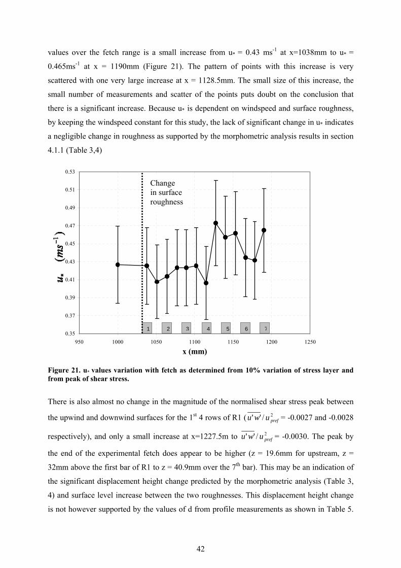
42
values over the fetch range is a small increase from u* = 0.43 ms-1 at x=1038mm to u* =
0.465ms-1 at x = 1190mm (Figure 21). The pattern of points with this increase is very
scattered with one very large increase at x = 1128.5mm. The small size of this increase, the
small number of measurements and scatter of the points puts doubt on the conclusion that
there is a significant increase. Because u* is dependent on windspeed and surface roughness,
by keeping the windspeed constant for this study, the lack of significant change in u* indicates
a negligible change in roughness as supported by the morphometric analysis results in section
4.1.1 (Table 3,4)
0.35
0.37
0.39
0.41
0.43
0.45
0.47
0.49
0.51
0.53
950 1000 1050 1100 1150 1200 1250
x (mm)
1 2 3 4 5 6 7
Change is surface roughness
Figure 21. u* values variation with fetch as determined from 10% variation of stress layer and from peak of shear stress.
There is also almost no change in the magnitude of the normalised shear stress peak between
the upwind and downwind surfaces for the 1st 4 rows of R1 ( 2/'' prefuwu = -0.0027 and -0.0028
respectively), and only a small increase at x=1227.5m to 2/'' prefuwu = -0.0030. The peak by
the end of the experimental fetch does appear to be higher (z = 19.6mm for upstream, z =
32mm above the first bar of R1 to z = 40.9mm over the 7th bar). This may be an indication of
the significant displacement height change predicted by the morphometric analysis (Table 3,
4) and surface level increase between the two roughnesses. This displacement height change
is not however supported by the values of d from profile measurements as shown in Table 5.
Change in surface roughness
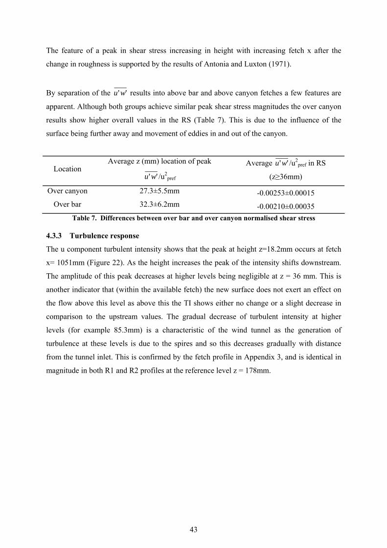
43
The feature of a peak in shear stress increasing in height with increasing fetch x after the
change in roughness is supported by the results of Antonia and Luxton (1971).
By separation of the ''wu results into above bar and above canyon fetches a few features are
apparent. Although both groups achieve similar peak shear stress magnitudes the over canyon
results show higher overall values in the RS (Table 7). This is due to the influence of the
surface being further away and movement of eddies in and out of the canyon.
Location Average z (mm) location of peak
''wu /u2pref
Average ''wu /u2pref in RS
(z≥36mm)
Over canyon 27.3±5.5mm -0.00253±0.00015 Over bar 32.3±6.2mm -0.00210±0.00035
Table 7. Differences between over bar and over canyon normalised shear stress 4.3.3 Turbulence response
The u component turbulent intensity shows that the peak at height z=18.2mm occurs at fetch
x= 1051mm (Figure 22). As the height increases the peak of the intensity shifts downstream.
The amplitude of this peak decreases at higher levels being negligible at z = 36 mm. This is
another indicator that (within the available fetch) the new surface does not exert an effect on
the flow above this level as above this the TI shows either no change or a slight decrease in
comparison to the upstream values. The gradual decrease of turbulent intensity at higher
levels (for example 85.3mm) is a characteristic of the wind tunnel as the generation of
turbulence at these levels is due to the spires and so this decreases gradually with distance
from the tunnel inlet. This is confirmed by the fetch profile in Appendix 3, and is identical in
magnitude in both R1 and R2 profiles at the reference level z = 178mm.

44
x (mm)
Tur
bule
nt I
nten
sity
12001150110010501000
0.35
0.30
0.25
0.20
0.15
0.10
0.05
Change in roughnessVariable
z = 21.0 mmz = 23.0 mmz = 25.0 mmz = 28.5 mmz = 32.0 mmz = 36.0 mmz = 40.9 mmz = 52.2 mmz = 66.8 mmz = 66.8 mm
z = 18.2 mm
z = 85.3 mmz = 109.0 mmz = 139.3 mmz = 178.0 mmz = 200.0 mm
z = 19.6 mm
1 2 3 4 5 6 7
Figure 22. Turbulent intensity u component over R1 type roughness including upstream values for comparison.
One reason for why the peak turbulent intensity doesn’t occur over the first bar can be found
by examination of the turbulent kinetic energy (TKE) budget. Near the surface the shear
production term usually makes a large contribution to the TKE budget and therefore the
turbulent intensity (equation 22) is due to relatively large ''wu values and strong wind shear.
However over the first bar there is positive shear stress and accelerated flow due to
convergence of flow lines. This positive shear stress combined with the decreased wind shear
at 18.2 mm (the bottom of the measurement range) leads to shear loss in the TKE budget.
However this counter gradient flux is most likely to be due to error in the velocity gradient
measurements as it is not physically meaningful to have a shear loss. It is likely that the high
turbulent intensity at x = 1051mm (1st canyon) is due to the divergence of streamlines (Figure
19) reducing velocity in the wake region (Figure 22) due to the decrease in pressure in
comparison to the upstream face of the bar leading to higher turbulent intensities at this point.
Because the R1 surface bars are closely spaced the flow over these elements is predicted by
the theories of Oke (1987) to be a skimming regime with a roughness length that is only
slightly different to the upstream Lego™ surface (see morphometric results, Table 3,4). Thus
it is likely that the turbulent intensities over R1 should not be much different in magnitude to

45
upstream. This is indicated as after the peak disturbance the turbulent intensity within the RS
(z ≤ 36mm) decreases approaching values found upstream (Figure 22). This decrease in
turbulent intensity is an indicator that this surface is not rougher as a rougher surface would
provide a consistently higher turbulent intensity close to the surface via enhanced TKE
production.
z (mm)
Tur
bule
nt I
nten
sity
12001150110010501000
0.20
0.15
0.10
0.05
Change in roughnessVariable
z = 21.0 mmz = 23.0 mmz = 25.0 mmz = 28.5 mmz = 32.0 mmz = 36.0 mmz = 40.9 mmz = 52.2 mmz = 66.8 mmz = 85.3 mm
z = 18.2 mm
z = 109.0 mmz = 139.3 mmz = 178.0 mmz = 200.0 mm
z = 19.6 mm
1 2 3 4 5 6 7
Figure 23. w component turbulent intensity including upstream values for comparison
Due to the influence of the surface the w component of turbulent intensity is smaller than the
u component. This surface influence is visible in Figure 23 with higher turbulent intensity
over the bars and comparatively lower turbulent intensity over the canyons. This influence
appears to extend up to a height of z = 23mm where the amplitude of this effect becomes
negligible. The w component follows a similar pattern to the u component with a peak at
1051mm, with the fastest decreases occurring at the low heights (e.g. z = 18.2mm). Over bars
5,6 the peak of turbulent intensity occurs at higher levels, for example z = 19.6 at bar 3, z =
21mm at bar 4 and z = 25 mm at bars 5,6 and canyon 6. However results close to the end of
this pattern are close to the end of the roughness and so may be adversely affected by the
approaching change in blockage coefficient.
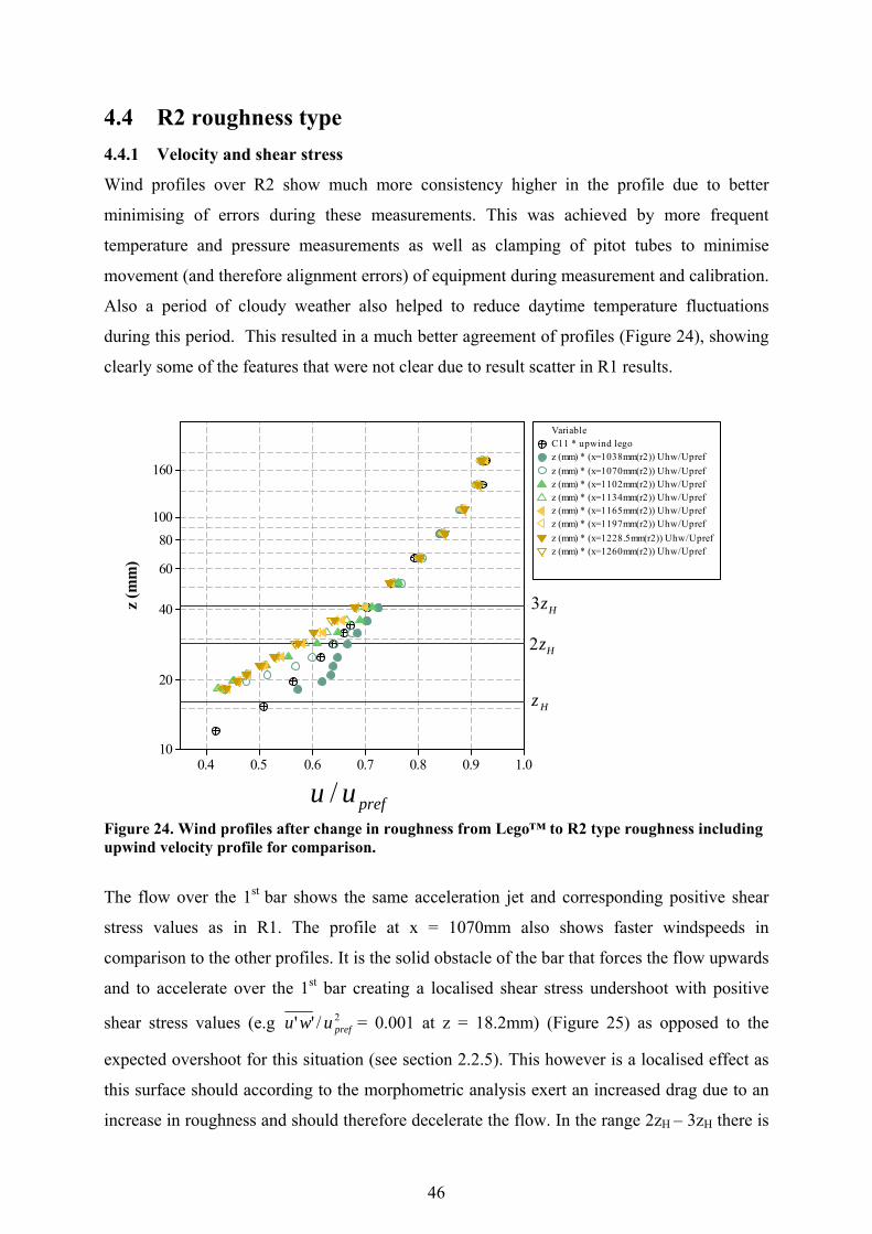
46
4.4 R2 roughness type 4.4.1 Velocity and shear stress
Wind profiles over R2 show much more consistency higher in the profile due to better
minimising of errors during these measurements. This was achieved by more frequent
temperature and pressure measurements as well as clamping of pitot tubes to minimise
movement (and therefore alignment errors) of equipment during measurement and calibration.
Also a period of cloudy weather also helped to reduce daytime temperature fluctuations
during this period. This resulted in a much better agreement of profiles (Figure 24), showing
clearly some of the features that were not clear due to result scatter in R1 results.
Uhw/Upref
z (m
m)
1.00.90.80.70.60.50.4
160
10080
60
40
20
10
Zh
2Zh
3Zh
Variable
z (mm) * (x=1134mm(r2)) Uhw/Uprefz (mm) * (x=1165mm(r2)) Uhw/Uprefz (mm) * (x=1197mm(r2)) Uhw/Uprefz (mm) * (x=1228.5mm(r2)) Uhw/Uprefz (mm) * (x=1260mm(r2)) Uhw/Upref
C11 * upwind legoz (mm) * (x=1038mm(r2)) Uhw/Uprefz (mm) * (x=1070mm(r2)) Uhw/Uprefz (mm) * (x=1102mm(r2)) Uhw/Upref
Figure 24. Wind profiles after change in roughness from Lego™ to R2 type roughness including upwind velocity profile for comparison.
The flow over the 1st bar shows the same acceleration jet and corresponding positive shear
stress values as in R1. The profile at x = 1070mm also shows faster windspeeds in
comparison to the other profiles. It is the solid obstacle of the bar that forces the flow upwards
and to accelerate over the 1st bar creating a localised shear stress undershoot with positive
shear stress values (e.g 2/'' prefuwu = 0.001 at z = 18.2mm) (Figure 25) as opposed to the
expected overshoot for this situation (see section 2.2.5). This however is a localised effect as
this surface should according to the morphometric analysis exert an increased drag due to an
increase in roughness and should therefore decelerate the flow. In the range 2zH – 3zH there is
prefuu /
Hz3
Hz2
Hz
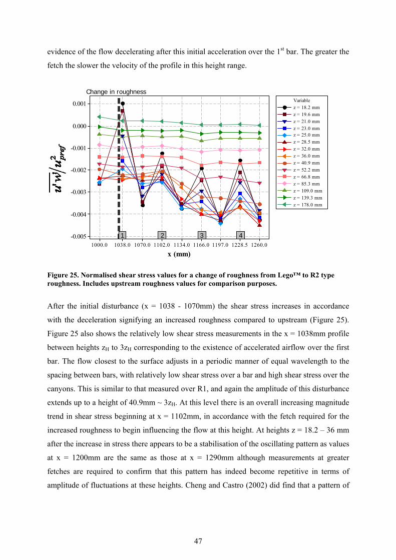
47
evidence of the flow decelerating after this initial acceleration over the 1st bar. The greater the
fetch the slower the velocity of the profile in this height range.
x (mm)
u'w
'/Upr
ef2
1260.01228.51197.01166.01134.01102.01070.01038.01000.0
0.001
0.000
-0.001
-0.002
-0.003
-0.004
-0.005
Change in roughnessVariable
z = 21.0 mmz = 23.0 mmz = 25.0 mmz = 28.5 mmz = 32.0 mmz = 36.0 mmz = 40.9 mmz = 52.2 mmz = 66.8 mmz = 85.3 mm
z = 18.2 mm
z = 109.0 mmz = 139.3 mmz = 178.0 mm
z = 19.6 mm
1 2 3 4
Figure 25. Normalised shear stress values for a change of roughness from Lego™ to R2 type roughness. Includes upstream roughness values for comparison purposes.
After the initial disturbance (x = 1038 - 1070mm) the shear stress increases in accordance
with the deceleration signifying an increased roughness compared to upstream (Figure 25).
Figure 25 also shows the relatively low shear stress measurements in the x = 1038mm profile
between heights zH to 3zH corresponding to the existence of accelerated airflow over the first
bar. The flow closest to the surface adjusts in a periodic manner of equal wavelength to the
spacing between bars, with relatively low shear stress over a bar and high shear stress over the
canyons. This is similar to that measured over R1, and again the amplitude of this disturbance
extends up to a height of 40.9mm ~ 3zH. At this level there is an overall increasing magnitude
trend in shear stress beginning at x = 1102mm, in accordance with the fetch required for the
increased roughness to begin influencing the flow at this height. At heights z = 18.2 – 36 mm
after the increase in stress there appears to be a stabilisation of the oscillating pattern as values
at x = 1200mm are the same as those at x = 1290mm although measurements at greater
fetches are required to confirm that this pattern has indeed become repetitive in terms of
amplitude of fluctuations at these heights. Cheng and Castro (2002) did find that a pattern of
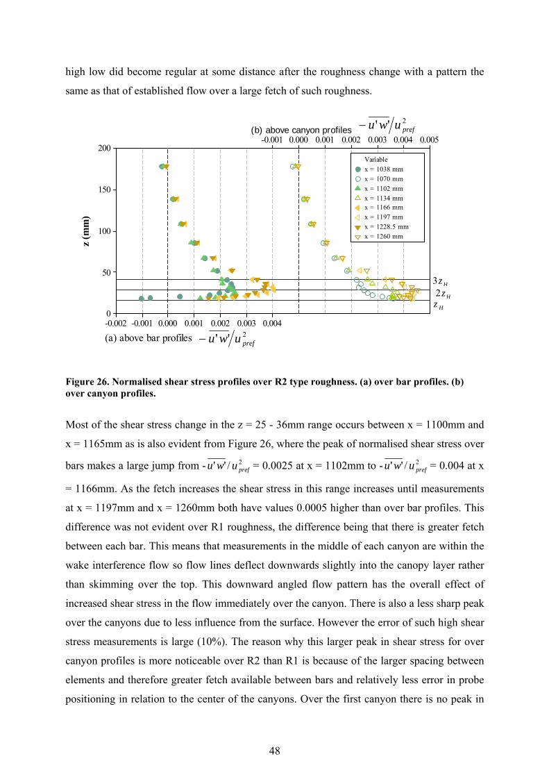
48
high low did become regular at some distance after the roughness change with a pattern the
same as that of established flow over a large fetch of such roughness.
-u'w'/Upref 2
-u'w'/Upref 2
z (m
m)
0.0040.0030.0020.0010.000-0.001-0.002
200
150
100
50
0
0.0050.0040.0030.0020.0010.000-0.001
Zh2Zh3Zh
Variable
x = 1166 mmx = 1197 mmx = 1228.5 mmx = 1260 mm
x = 1038 mmx = 1070 mmx = 1102 mmx = 1134 mm
(a) above bar profiles
(b) above canyon profiles
Figure 26. Normalised shear stress profiles over R2 type roughness. (a) over bar profiles. (b) over canyon profiles.
Most of the shear stress change in the z = 25 - 36mm range occurs between x = 1100mm and
x = 1165mm as is also evident from Figure 26, where the peak of normalised shear stress over
bars makes a large jump from - 2/'' prefuwu = 0.0025 at x = 1102mm to - 2/'' prefuwu = 0.004 at x
= 1166mm. As the fetch increases the shear stress in this range increases until measurements
at x = 1197mm and x = 1260mm both have values 0.0005 higher than over bar profiles. This
difference was not evident over R1 roughness, the difference being that there is greater fetch
between each bar. This means that measurements in the middle of each canyon are within the
wake interference flow so flow lines deflect downwards slightly into the canopy layer rather
than skimming over the top. This downward angled flow pattern has the overall effect of
increased shear stress in the flow immediately over the canyon. There is also a less sharp peak
over the canyons due to less influence from the surface. However the error of such high shear
stress measurements is large (10%). The reason why this larger peak in shear stress for over
canyon profiles is more noticeable over R2 than R1 is because of the larger spacing between
elements and therefore greater fetch available between bars and relatively less error in probe
positioning in relation to the center of the canyons. Over the first canyon there is no peak in
2'' prefuwu−
2'' prefuwu−
Hz3Hz2
Hz
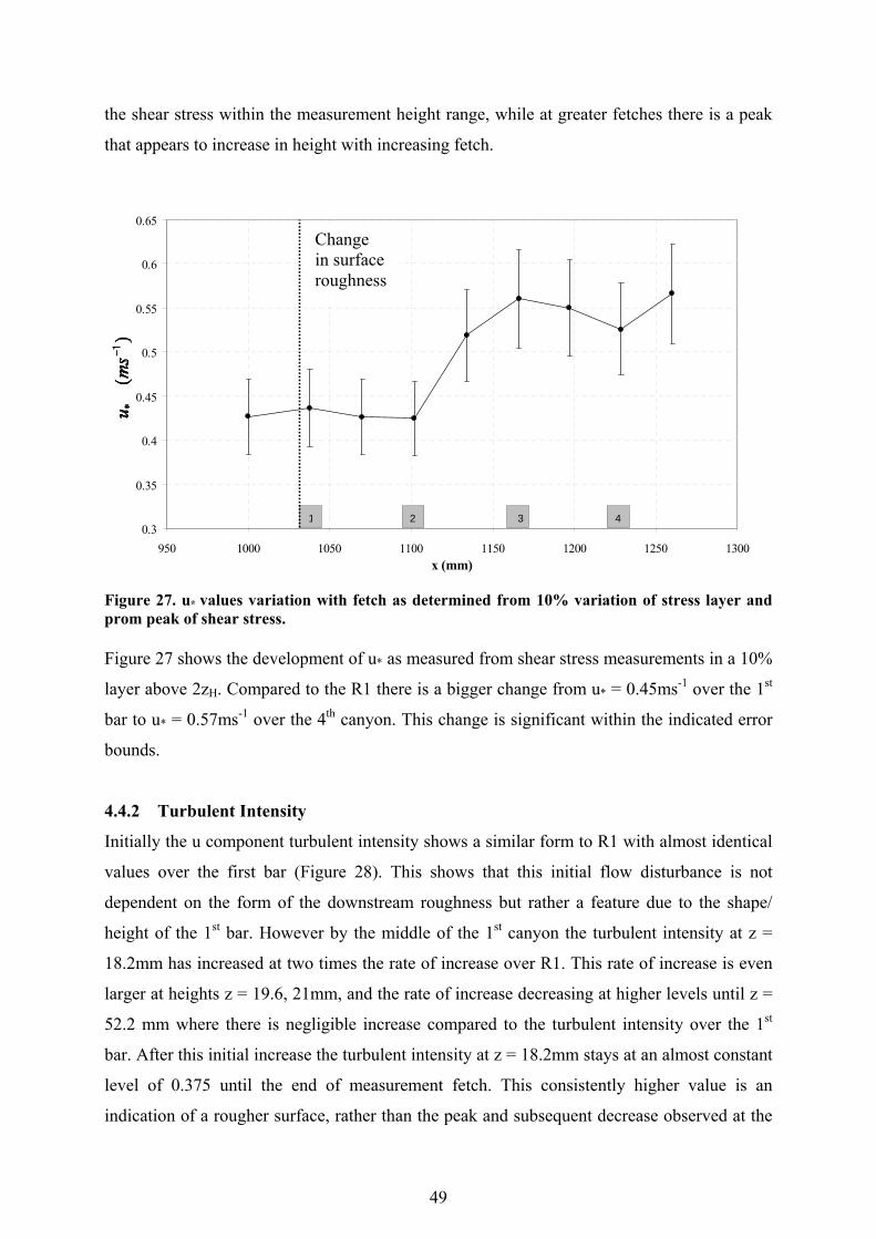
49
the shear stress within the measurement height range, while at greater fetches there is a peak
that appears to increase in height with increasing fetch.
0.3
0.35
0.4
0.45
0.5
0.55
0.6
0.65
950 1000 1050 1100 1150 1200 1250 1300x (mm)
1 2 3 4
Change is surface roughness
Figure 27. u* values variation with fetch as determined from 10% variation of stress layer and prom peak of shear stress. Figure 27 shows the development of u* as measured from shear stress measurements in a 10%
layer above 2zH. Compared to the R1 there is a bigger change from u* = 0.45ms-1 over the 1st
bar to u* = 0.57ms-1 over the 4th canyon. This change is significant within the indicated error
bounds.
4.4.2 Turbulent Intensity
Initially the u component turbulent intensity shows a similar form to R1 with almost identical
values over the first bar (Figure 28). This shows that this initial flow disturbance is not
dependent on the form of the downstream roughness but rather a feature due to the shape/
height of the 1st bar. However by the middle of the 1st canyon the turbulent intensity at z =
18.2mm has increased at two times the rate of increase over R1. This rate of increase is even
larger at heights z = 19.6, 21mm, and the rate of increase decreasing at higher levels until z =
52.2 mm where there is negligible increase compared to the turbulent intensity over the 1st
bar. After this initial increase the turbulent intensity at z = 18.2mm stays at an almost constant
level of 0.375 until the end of measurement fetch. This consistently higher value is an
indication of a rougher surface, rather than the peak and subsequent decrease observed at the
Change in surface roughness

50
same height over R1. Compared to the downstream values at z = 19.6mm there is a jump in
turbulent intensity from 0.265 over the 1st bar to a consistent 0.355 over the rest of the
measurement fetch. This could be a result of the changing surface level (+1.7mm), but even
when this is taken into account by estimating the turbulent intensity values at z = 19.6 + 1.7 =
21.3mm the increase of turbulent intensity is + 0.06. There is the displacement height to
consider as morphometric analysis of Macdonald et al. (1998) predicts an increase of 3.5mm,
although profile measurements over the Lego™ did not support this. The combination of
surface level and displacement height change may displace the flow vertically by up to
5.2mm, which gives a equivalent height z = 19.6 + 5.2 = 24.8mm. By estimating from values
at z = 25mm (due to the large errors in turbulent intensity measurement and displacement
height uncertainties this assumption is not significant) the turbulent intensity at the end of the
measurement length is 0.30, an increase of 0.03 from the upstream value. The above
assumptions do however assume that the readjustment of the flow to the new surface at this
height has occurred within the available fetch which is not the case as the turbulent intensity
is still increasing at this level. An experiment with a longer measurement fetch would be
required to confirm if this is occurring.
x (mm)
Tur
bule
nt I
nten
sity
1260.01228.51197.01166.01134.01102.01070.01038.01000.0
0.40
0.35
0.30
0.25
0.20
0.15
0.10
0.05
Roughness changeVariable
z = 21 mmz = 23 mmz = 25 mmz = 28.5 mmz = 32 mmz = 36 mmz = 40.9 mmz = 52.2 mmz = 66.8 mmz = 85.3 mm
z = 18.2 mm
z = 109 mmz = 139.3 mmz = 178 mm
z = 19.6 mm
1 2 3 4
Figure 28. Turbulent intensity u component over R2 type roughness including upstream values for comparison.

51
The w component turbulent intensity at height z = 18.2, 19.6mm (Figure 29) also shows an
increase which is twice as large as compared to that observed over R1 (Figure 23). The same
periodic pattern as over R1 is observed although the larger spacing between bars makes this
more pronounced, with a amplitude between low and high that is approximately four times
larger than over R1 at z = 18.2mm. The height at which this amplitude becomes negligible is
z = 23mm in agreement with the R1 roughness.
The turbulent intensity rate of increase of u and w components becomes less and less at higher
levels until z = 66.8mm where the trend becomes a decreasing one. This is a feature of the
wind tunnel turbulent intensity variation with fetch as discussed in section 4.2.3. Another
indicator that this is not an effect of the roughness change is that this effect is the same
magnitude over both R1 and R2 roughness.
x (mm)
Tur
bule
nt I
nten
sity
126012281197116611341102107010381000
0.20
0.15
0.10
0.05
Change in roughnessVariable
z = 21 mmz = 23 mmz = 25 mmz = 28.5 mmz = 32 mmz = 36 mmz = 40.9 mmz = 52.2 mmz = 66.8 mmz = 85.3 mm
z = 18.2 mm
z = 109 mmz = 139.3 mmz = 178 mm
z = 19.6 mm
1 2 3 4
Figure 29. Turbulent intensity w component over R2 type roughness including upstream values for comparison.
4.4.3 IBL height.
The IBL height is only calculated for the R2 surface roughness as the velocity profiles are
more consistent than those over R1, and therefore easier to interpret. The results of the shear
stress (Figure 25) appear to show that the RS extends up to 3zH and the velocity profiles are
characteristic of the upwind surface above this height. Thus the equilibrium layer does not
extend above the RS and so it is not possible to determine the downwind log law parameters

52
z02 and d2 by profile measurements. However the d2 and z02 values as determined by the
morphometric analysis can be used to estimate the IBL height.
0
10
20
30
40
50
60
70
80
90
1000 1050 1100 1150 1200 1250 1300
x (mm)
IBL
hei
ght (
mm
)
Elliot (1958) IBL height (log law:R2)Elliot (1958) IBL height (Morphology:R2)Wood (1982) IBL height R2Panofsky and Dutton (1984) IBL height R2inflection R2intersection R2
R2 Surface level
Figure 30. IBL growth after a change in surface roughness from Lego™ to R2.
The IBL heights were obtained by measuring height of inflection (δi2) of the downstream
influenced wind profile and the upstream influenced flow. The method of using the point of
intersection between the upwind and downwind profiles (δi) was also used for comparison
although its application is not strictly valid as the downstream profile is in the RS and
dependent on surface form. Overall as predicted in section 2.2.2 δi gives larger values of IBL
height (see Figure 30). It is noted that the error of these measurements is large (±6mm) due to
curve fitting errors and the difficulty in interpreting the inflection point. The theories of Elliot,
1958 (Equation 7); Wood, 1982 (Equation 9); Panofsky and Dutton, 1984 (Equation 10) are
presented using roughness parameters calculated using upstream and downstream z0
parameters obtained using the morphometric analysis of Macdonald et al. (1998)(Figure 30)
as well as upstream z0 values obtained from the log profile fit using u*(IS). Elliot’s (1958)
theory shows the best agreement with the experimental results although the limited fetch

53
range of experimental results and large errors make it difficult to make any conclusions about
the growth at longer fetches. Panofsky and Dutton (1984) show reasonably good agreement
with the rate of increase of the experimentally derived IBL height. Wood’s (1982) theory
gives a very slow estimation of IBL growth in comparison to the above theories and the
results obtained, as found by Savelyev and Taylor (2005) in their review paper. The effect of
using z0 from the log law fit using u*(IS) for the upstream profile is also shown in Figure 30,
leading to a slightly slower IBL growth rate as compared to that obtained from purely
morphometric results.
0
10
20
30
40
50
60
70
80
90
1000 1050 1100 1150 1200 1250 1300
x (mm)
IBL
hei
ght (
mm
)
Elliot (1958) IBL height (log law:R2)Elliot (1958) IBL height (Morphology:R2)Wood (1982) IBL height R2Panofsky and Dutton (1984) IBL height R2inflection R2intersection R2
R2 Surface level
Figure 31. IBL growth after a change in surface roughness from Lego™ to R2 including consideration of displacement height change The displacement height is not considered in any of the theories presented, but as it is a large
percentage of the calculated IBL depth the experimental results can be adjusted by taking the
surface level as equal to (d2 –d1) (d2 = 3.5mm from morphometric analysis of Macdonald et al.
1998). The effect of this is to give a larger IBL depth in relation to the surface, bringing
Panofsky and Dutton’s (1984) theory into better agreement with the experimental results
(Figure 31).

54
4.4.4 Shear stress overshoot
The theoretical shear stress overshoot as described by Barlow (personal communication) and
Jensen (1978) are calculated using the IBL height predictions of Elliot (1958) as these appear
to be closest to the experimental results obtained above. The values of upstream and
downstream z0 and d are those predicted by the morphometric analysis of Macdonald et al.
(1998), as this means a consistent theory is used for both surfaces. The results of these
theories are displayed in Figure 32. Both Jensen (1978) and Barlow (unpublished) predict
shear stress overshoot, with the peak of overshoot occurring at 1mm downstream of the start
of the roughness change for Jensen (1978) and 8mm downstream for Barlow (unpublished).
The value of the peak is not critical as both theories predict infinite shear stress ratio’s at
particular IBL depths, for example Barlow (personal communication) asymptotes when
( ) 012 zdi =−δ .
0
1
2
3
4
5
6
7
8
1032 1082 1132 1182 1232x (mm)
τ 2/τ
1
Barlow (personal communication)Jensen, 1978This experiment R2
Figure 32. Shear stress overshoot as predicted by the theories of Barlow (unpublished) and Jensen (1978), for a change in roughness of Lego™ to R2 using the values of upstream and downstream z0 and d as calculated using the morphometric analysis of Macdonald et al. (1998) and IBL height values of Elliot (1958).
55
The predictions in Figure 32 do not agree with the results obtained from a 10% variation in
shear stress layer above z=2zH. However the values of shear stress measured are highly height
dependent. The location of a large overshoot over the first bar of R2 is not evident within the
height range of this experiment, and it was actually found that for this change in roughness
resulted in a decrease of shear stress over this bar due to the acceleration of flow. This is due
to using a 2D roughness element and measurements over 3D roughness changes could give
different results although this would be difficult unless a larger wind tunnel was used as
spatial averaging would be required. The measurement of shear stress overshoot is also likely
to depend on the measurement technique used as direct measurements using pressure tapping
(Antonia and Luxton, 1971) or drag plates (Bradley, 1968) have clearly revealed overshoot,
avoiding the difficulties of above surface shear stress spatial inhomogenities.
5 Conclusions The first part of the experiment was to create and verify against atmospheric observations a
boundary layer in the wind tunnel. The upstream flow was found to be consistent with the log
wind law, and turbulent intensity in good agreement with that expected for a rough surface
(VDI, 2000). The turbulent energy spectra is in accordance with the results of Kaimal et
al.(1972) in the u component but with too much energy in the w and v components. The RS
was found to extend up to 2zH and assuming that a 10% variation in shear stress above this is
considered constant the IS is found to extend from 2zH to 3zH. From log profile measurements
within this height range the log law parameters z01 and d1 were deduced and found to be much
larger than predicted by morphometric analysis methods. This is considered to be a result of
the artificial generation of turbulence by spires, and similarly excessive d values have been
reported from using this method in the wind tunnel study of Cheng and Castro, 2002. Also the
error due to high turbulence corresponds to an underestimate of shear stress compared to the
true values, thus giving artificially high d values during the curve fitting process. u* values
were also obtained by using shear stress measurements in the RS and by best fitting all profile
parameters simultaneously which gave consistent results within the bounds of error.
Two different changes in surface roughness were considered, both 2D in structure. This
surface structure results in a periodic variation of shear stress and w component turbulent
intensity with fetch. This periodic variation has wavelength equal to the bar spacing and an
amplitude that decreases with height. A commonly observed feature of previous roughness
56
change experiments is a shear stress overshoot, which is not observed in this experiment.
However it is found that the shear stress variation with fetch is highly dependent on the height
at which it is measured. Another consideration is the experimental method as almost all
previous experiments that have observed this shear overshoot have used direct measurements
of momentum flux on the surface by means of drag plates or pressure tapping. However
previous experiments have often used roughness changes of much larger magnitude M than
studied here and 3D surface morphology, which due to the spatial averaging required over 3D
element structures, needs a larger wind tunnel.
The shear stress overshoot was theoretically predicted by two separate theories to be located
over the 1st bar of the downstream roughness which due to the particular form of the change
in this study actually had a localised effect of reducing the stress over this location due to the
presence of a jet. Thus the existence of an overshoot is dependent on the form of the
roughness change and may still be a feature of changes to 3D surface roughness. The scale of
the wind tunnel also may play a role as to provide a rougher surface the downstream bar
roughness height (zH) has to be large (16% of the boundary layer depth).
The upstream surface in this experiment works in combination with the turbulence producing
spires and so its roughness cannot be changed without extensive experimentation, the
disadvantage being that is actually relatively rough and so it is difficult to create a surface of
higher roughness whose elements are not excessively large as a fraction of the boundary
layer. Elements that are too large have a large blockage coefficient which has the effect of
speeding the up the flow in the test section which is undesirable because this is not a feature
associated with full scale experiments and therefore makes comparison of results difficult.
The differences between the two downstream roughness was a due to changing the ratio of
element height to canyon width ratio, with R1 having a 1:1 ratio and R2 setup to obtain
maximum z0 values with a 1:4 ratio. The effect of these two ratios had a large effect on the
turbulent response, with the turbulent intensity over R2 of both u and w components in the RS
initially experiencing an increase twice the magnitude of that at the same heights over R1.
After this initial turbulent intensity increase a decrease was measured with increasing fetch
over R1 suggesting that the initial increase was a localised feature caused by the flow
encountering the first bar roughness. In comparison the turbulent intensity at the same levels
over the R2 roughness were consistently higher than those over R1 suggesting an increase in
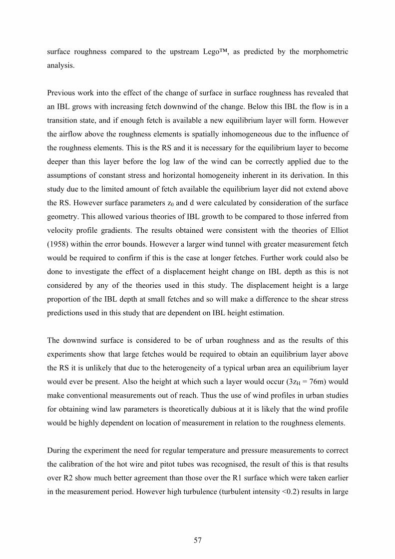
57
surface roughness compared to the upstream Lego™, as predicted by the morphometric
analysis.
Previous work into the effect of the change of surface in surface roughness has revealed that
an IBL grows with increasing fetch downwind of the change. Below this IBL the flow is in a
transition state, and if enough fetch is available a new equilibrium layer will form. However
the airflow above the roughness elements is spatially inhomogeneous due to the influence of
the roughness elements. This is the RS and it is necessary for the equilibrium layer to become
deeper than this layer before the log law of the wind can be correctly applied due to the
assumptions of constant stress and horizontal homogeneity inherent in its derivation. In this
study due to the limited amount of fetch available the equilibrium layer did not extend above
the RS. However surface parameters z0 and d were calculated by consideration of the surface
geometry. This allowed various theories of IBL growth to be compared to those inferred from
velocity profile gradients. The results obtained were consistent with the theories of Elliot
(1958) within the error bounds. However a larger wind tunnel with greater measurement fetch
would be required to confirm if this is the case at longer fetches. Further work could also be
done to investigate the effect of a displacement height change on IBL depth as this is not
considered by any of the theories used in this study. The displacement height is a large
proportion of the IBL depth at small fetches and so will make a difference to the shear stress
predictions used in this study that are dependent on IBL height estimation.
The downwind surface is considered to be of urban roughness and as the results of this
experiments show that large fetches would be required to obtain an equilibrium layer above
the RS it is unlikely that due to the heterogeneity of a typical urban area an equilibrium layer
would ever be present. Also the height at which such a layer would occur (3zH = 76m) would
make conventional measurements out of reach. Thus the use of wind profiles in urban studies
for obtaining wind law parameters is theoretically dubious at it is likely that the wind profile
would be highly dependent on location of measurement in relation to the roughness elements.
During the experiment the need for regular temperature and pressure measurements to correct
the calibration of the hot wire and pitot tubes was recognised, the result of this is that results
over R2 show much better agreement than those over the R1 surface which were taken earlier
in the measurement period. However high turbulence (turbulent intensity <0.2) results in large

58
errors in shear stress, velocity and turbulent intensity. One aspect for future study would be to
implement an error correction scheme to minimise these cross wire related errors.

59
Appendices Appendix 1. Location of profile measurements over Lego™ surface
roughness
Appendix 2. Rejected Lego™ wind profiles.
0
20
40
60
80
100
120
140
160
180
200
0 0.1 0.2 0.3 0.4 0.5 0.6 0.7 0.8 0.9 1
z (m
m)
x=1128mmx=1076mmx=1055mmx=1078mmx=1042mmx=1074mmx=991mmx=955mm
Figure 2A. Lego™ wind profiles rejected due to large temperature related errors.
x=955mm x=991mm
x=1042mm
x=1051mmx=1055mm
x=1074mm
x=1076mm
x=1078mm
x=1128mm
x=1202mm
Profiles not used
Profiles included
Figure 1A. Location of profile measurements over Lego™ surface roughness
prefuu /

60
Appendix 3. Change in normalisation wind speed with fetch
0.9
0.91
0.92
0.93
0.94
0.95
0.96
0.97
0.98
0.99
1
900 950 1000 1050 1100 1150 1200 1250 1300
x (mm) Figure 3A. Change in normalised velocity with fetch at z=178mm over Lego™ surface roughness.
0.9
0.91
0.92
0.93
0.94
0.95
0.96
0.97
0.98
0.99
1
900
920
940
960
980
1000
1020
1040
1060
1080
1100
1120
1140
1160
1180
1200
1220
1240
x (mm)
0
0.01
0.02
0.03
0.04
0.05
0.06
0.07
0.08
Tur
bule
nt In
tens
ity
Uhw/Uprefturbulent intensity
Change in surface roughness
R1Lego
Figure 3B. Change in normalisation wind speed and turbulent intensity with fetch over change in surface roughness form Lego™ to R1, measured at z=178mm.
prefuu /
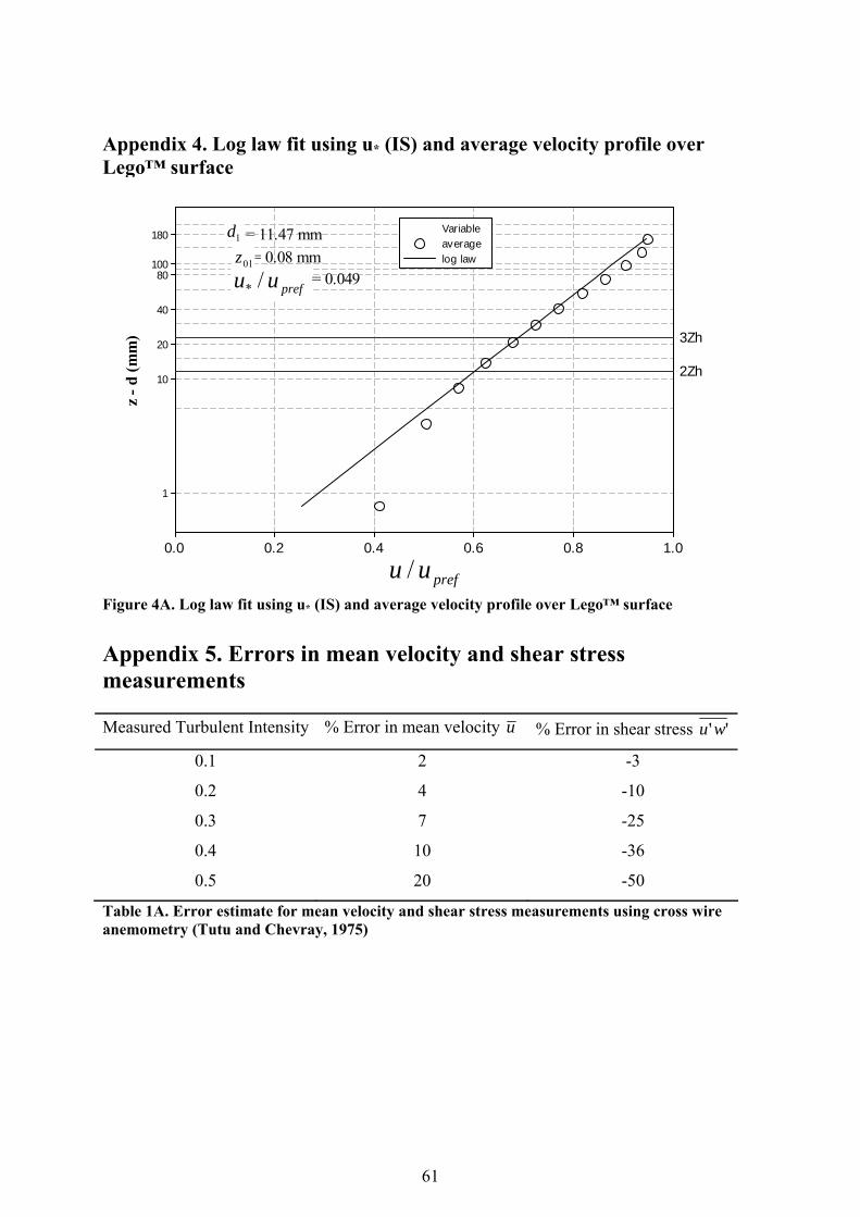
61
Appendix 4. Log law fit using u* (IS) and average velocity profile over Lego™ surface
Uhw/Upref
z - d
(mm
)
1.00.80.60.40.20.0
180
10080
40
20
10
1
2Zh
3Zh
Variableaveragelog law
d = 11.47 mmz0 = 0.08 mmustar/Upref = 0.049
Figure 4A. Log law fit using u* (IS) and average velocity profile over Lego™ surface Appendix 5. Errors in mean velocity and shear stress measurements Measured Turbulent Intensity % Error in mean velocity u % Error in shear stress ''wu
0.1 2 -3
0.2 4 -10
0.3 7 -25
0.4 10 -36
0.5 20 -50
Table 1A. Error estimate for mean velocity and shear stress measurements using cross wire anemometry (Tutu and Chevray, 1975)
prefuu /
prefuu /*
01z1d

62
References ANTONIA, R. A. and LUXTON, R. E., (1971). The response of a turbulent boundary layer to a step change in surface roughness. Part 1. Smooth to Rough. Journal of Fluid Mechanics, 48, 721-761. BRADLEY, E. F., (1968). A micrometeorological study of velocity profiles and surface drag in the region modified by a change in surface roughness. Quarterly Journal of the Royal Meteorological Society, 94, 361-379. BRUUN, H. H., (1995). Hot-wire anemometry. Oxford University press. 536pp. CHENG, H. and CASTRO, I. P., (2002). Near wall flow over urban-like roughness. Boundary-Layer Meteorology, 104, 229-259. COOK, N. J., (1978). Wind-tunnel simulation of the adiabatic atmospheric boundary layer by roughness, barrier and mixing-device methods. Journal of Industrial Aerodynamics, 3, 157-176. COUNIHAN, J., (1971). Wind tunnel determination of the roughness length as a function of the fetch and the roughness density of three-dimensional roughness elements. Atmospheric Environment, 5, 637-642. ELLIOT, W. P., (1958). The growth of the atmospheric internal boundary layer. Transactions of the American Geophysical Union, 39, 1048-1054. ESDU, (1986). Mean fluid forces and moments on rectangular prisms: surface-mounted structures in turbulent shear flow. Engineering Sciences Data Item number 8003. GARRATT, J. R. (1992). The atmospheric boundary layer. Cambridge University Press, 316pp. GRIMMOND, C.S.B. and OKE, T. R., (1999). Aerodynamic properties of urban areas derived from analysis of surface form. Journal of Applied Meteorology, 38, 1262-1292. JACKSON, P. S., (1981). On the displacement height in the logarithmic velocity profile. Journal of Fluid Mechanics, 111, 15-25. JENSEN, N. O., (1978). Change of surface roughness and the planetary boundary layer. Quarterly Journal of the Royal Meteorological Society, 104, 351-356. JØRGENSEN, F. E., (2002). How to measure turbulence with hot wire anemometers – a practical guide. Dantec Dynamics, P.O. Box 121, Tonsbakken 16-18, DK-2740 Skovlunde, Denmark. KADER, B. A., (1977). Hydraulic resistance of surfaces covered by two-dimensional roughness at high reynolds numbers. Teoreticheskie Osnovy Khimicheskoi Tekhnologii, 11, 393-404.

63
KAIMAL, J. C. and FINNIGAN, J. J., (1994). Atmospheric boundary layer Flows, Their structure and management. Oxford University press. 289pp. KAIMAL, J. C., WYNGAARD, J. C., IZUMI, Y., COTE, O. R., (1972). Spectral characteristics of surface level turbulence. Quarterly Journal of the Royal Meteorological Society, 98, No 417, 563-589. KUTZBACH, J. E., (1961). Investigations of the modification of wind profiles by artificially controlled surface roughness. University of Wisconsin Department of Meteorology annual report, 71-113 LEONARDI1, S., ORLANDI, P., SMALLEY, R. J., DJENIDI, I., ANTONIA, R. A., (2003). Direct numerical simulations of turbulent channel flow with transverse square bars on one wall. Journal of Fluid Mechanics, 491, 229–238. LETTAU, H., (1969). Note on aerodynamic roughness-parameter estimation on the basis of roughness-element description. Journal of Applied Meteorology, 8, 828-829. MACDONALD, R. W., GRIFFITHS, R. F., HALL, D. J., (1998). An improved method for estimation of surface roughness of obstacle arrays. Atmospheric Environment, 32, 1857–1864. MIYAKE, M., (1965). Transformation of the atmospheric boundary layer over inhomogeneous surfaces, Science Reports 5R-6, University of Washington, Seattle, U.S.A. MULHEARN, P. J., (1978). A wind tunnel boundary-layer study of the effects of a surface roughness change: Rough to smooth. Boundary-Layer Meteorology, 15, 3-30. OKE, T. K., (1987). Boundary layer climates: 2nd Edition. Routeledge, UK. PENDERGRASS, W. and ARYA, S. P. S., (1984). Dispersion in the neutral boundary layer over a step change in surface roughness – I. Mean flow and turbulence structure. Atmospheric Environment, 18, 1267-1279. RAO, J. S., WYNGAARD, J. C., COTE, O. R., (1974). The structure of the two-dimensional internal boundary layer over a sudden change of surface roughness. Journal of Atmospheric Sciences, 31,738-746. RAUPACH, M. R., ANTONIA, R. A., RAJAGOPALAN, S., (1991). Rough-Wall turbulent boundary layers. Applied Mechanics Review, 44, 1-25. RAUPACH, M. R., THOM, A. S., EDWARDS, I., (1980). A wind tunnel study of turbulent flow close to regularly arrayed rough surfaces. Boundary-Layer Meteorology, 18, 373-397. SAVELYEV, S. A., TAYLOR, P. A., (2005). Internal boundary layers: I. Height formulae for neutral and diabatic flows. Boundary-Layer Meteorology, 115, 1-25. SINI, J. F., ANQUETIN, S., MESTAYER, P., (1996). Pollutant dispersion and thermal effects in urban street canyons’, Atmospheric Environment, 30, 2659–2677.

64
TUTU, N. K. and CHEVRAY, R., (1975). Cross-wire anemometry in high intensity turbulence. Journal of Fluid Mechanics, 71, 785-800. VDI RICHTLINIE3783, Blatt 12, (2000). Umweltmeteorologie. Physikalische modellierung von stromungs- und ausbreitungsvorgangen in der atmospharischen grenzschicht. VDI Handbuch Reinhaltung der Luft, Band 1b. WALMSLEY, J. L., (1989). Internal boundary-layer height formulae – A comparison with atmospheric data. Boundary-Layer Meteorology, 47, 251- 262. WIERINGA, J., (1993). Representative roughness parameters for homogeneous terrain. Boundary-Layer Meteorology. 63, 323-363.