boundary-layer transition results from the f-16xl-2 ... · boundary-layer transition results ......

NASA/TM-1999-209013

Boundary-Layer Transition Results From the F-16XL-2 Supersonic Laminar Flow Control Experiment

Laurie A. MarshallNASA Dryden Flight Research CenterEdwards, California

December 1999

The NASA STI Program Office…in Profile

Since its founding, NASA has been dedicatedto the advancement of aeronautics and space science. The NASA Scientific and Technical Information (STI) Program Office plays a keypart in helping NASA maintain thisimportant role.

The NASA STI Program Office is operated byLangley Research Center, the lead center forNASA’s scientific and technical information.The NASA STI Program Office provides access to the NASA STI Database, the largest collectionof aeronautical and space science STI in theworld. The Program Office is also NASA’s institutional mechanism for disseminating theresults of its research and development activities. These results are published by NASA in theNASA STI Report Series, which includes the following report types:

• TECHNICAL PUBLICATION. Reports of completed research or a major significantphase of research that present the results of NASA programs and include extensive dataor theoretical analysis. Includes compilations of significant scientific and technical data and information deemed to be of continuing reference value. NASA’s counterpart of peer-reviewed formal professional papers but has less stringent limitations on manuscriptlength and extent of graphic presentations.

• TECHNICAL MEMORANDUM. Scientificand technical findings that are preliminary orof specialized interest, e.g., quick releasereports, working papers, and bibliographiesthat contain minimal annotation. Does notcontain extensive analysis.

• CONTRACTOR REPORT. Scientific and technical findings by NASA-sponsored contractors and grantees.

• CONFERENCE PUBLICATION. Collected papers from scientific andtechnical conferences, symposia, seminars,or other meetings sponsored or cosponsoredby NASA.

• SPECIAL PUBLICATION. Scientific,technical, or historical information fromNASA programs, projects, and mission,often concerned with subjects havingsubstantial public interest.

• TECHNICAL TRANSLATION. English- language translations of foreign scientific and technical material pertinent toNASA’s mission.

Specialized services that complement the STIProgram Office’s diverse offerings include creating custom thesauri, building customizeddatabases, organizing and publishing researchresults…even providing videos.

For more information about the NASA STIProgram Office, see the following:

• Access the NASA STI Program Home Pageat

http://www.sti.nasa.gov

• E-mail your question via the Internet to [email protected]

• Fax your question to the NASA Access HelpDesk at (301) 621-0134

• Telephone the NASA Access Help Desk at(301) 621-0390

• Write to:NASA Access Help DeskNASA Center for AeroSpace Information7121 Standard DriveHanover, MD 21076-1320

NASA/TM-1999-209013


Laurie A. MarshallNASA Dryden Flight Research CenterEdwards, California

December 1999

National Aeronautics andSpace Administration

Dryden Flight Research CenterEdwards, California 93523-0273

NOTICE

Use of trade names or names of manufacturers in this document does not constitute an official endorsementof such products or manufacturers, either expressed or implied, by the National Aeronautics andSpace Administration.

Available from the following:

NASA Center for AeroSpace Information (CASI) National Technical Information Service (NTIS)7121 Standard Drive 5285 Port Royal RoadHanover, MD 21076-1320 Springfield, VA 22161-2171(301) 621-0390 (703) 487-4650

CONTENTS

Page

ABSTRACT . . . . . . . . . . . . . . . . . . . . . . . . . . . . . . . . . . . . . . . . . . . . . . . . . . . . . . . . . . . . . . . . . . . . . . . 1

NOMENCLATURE . . . . . . . . . . . . . . . . . . . . . . . . . . . . . . . . . . . . . . . . . . . . . . . . . . . . . . . . . . . . . . . . . 1

INTRODUCTION . . . . . . . . . . . . . . . . . . . . . . . . . . . . . . . . . . . . . . . . . . . . . . . . . . . . . . . . . . . . . . . . . . 2

AIRCRAFT DESCRIPTION . . . . . . . . . . . . . . . . . . . . . . . . . . . . . . . . . . . . . . . . . . . . . . . . . . . . . . . . . . 3

EXPERIMENT DESCRIPTION . . . . . . . . . . . . . . . . . . . . . . . . . . . . . . . . . . . . . . . . . . . . . . . . . . . . . . . 3Design Flight Conditions . . . . . . . . . . . . . . . . . . . . . . . . . . . . . . . . . . . . . . . . . . . . . . . . . . . . . . . . . 4Design Pressure Distribution . . . . . . . . . . . . . . . . . . . . . . . . . . . . . . . . . . . . . . . . . . . . . . . . . . . . . . 4Wing Glove . . . . . . . . . . . . . . . . . . . . . . . . . . . . . . . . . . . . . . . . . . . . . . . . . . . . . . . . . . . . . . . . . . . 4Suction System. . . . . . . . . . . . . . . . . . . . . . . . . . . . . . . . . . . . . . . . . . . . . . . . . . . . . . . . . . . . . . . . . 4Shock Fences . . . . . . . . . . . . . . . . . . . . . . . . . . . . . . . . . . . . . . . . . . . . . . . . . . . . . . . . . . . . . . . . . . 5Turbulence Diverter . . . . . . . . . . . . . . . . . . . . . . . . . . . . . . . . . . . . . . . . . . . . . . . . . . . . . . . . . . . . . 5Excrescences . . . . . . . . . . . . . . . . . . . . . . . . . . . . . . . . . . . . . . . . . . . . . . . . . . . . . . . . . . . . . . . . . . 6

INSTRUMENTATION . . . . . . . . . . . . . . . . . . . . . . . . . . . . . . . . . . . . . . . . . . . . . . . . . . . . . . . . . . . . . . 6Pressure Taps . . . . . . . . . . . . . . . . . . . . . . . . . . . . . . . . . . . . . . . . . . . . . . . . . . . . . . . . . . . . . . . . . . 6Mass Flow Sensors . . . . . . . . . . . . . . . . . . . . . . . . . . . . . . . . . . . . . . . . . . . . . . . . . . . . . . . . . . . . . 7Hot-Film Anemometers . . . . . . . . . . . . . . . . . . . . . . . . . . . . . . . . . . . . . . . . . . . . . . . . . . . . . . . . . . 7Data Recording. . . . . . . . . . . . . . . . . . . . . . . . . . . . . . . . . . . . . . . . . . . . . . . . . . . . . . . . . . . . . . . . . 7Interpretation of Hot-Film Signals . . . . . . . . . . . . . . . . . . . . . . . . . . . . . . . . . . . . . . . . . . . . . . . . . . 8

TEST CONDITIONS . . . . . . . . . . . . . . . . . . . . . . . . . . . . . . . . . . . . . . . . . . . . . . . . . . . . . . . . . . . . . . . . 8

RESULTS . . . . . . . . . . . . . . . . . . . . . . . . . . . . . . . . . . . . . . . . . . . . . . . . . . . . . . . . . . . . . . . . . . . . . . . . . 9Shock Fence . . . . . . . . . . . . . . . . . . . . . . . . . . . . . . . . . . . . . . . . . . . . . . . . . . . . . . . . . . . . . . . . . . . 9Pressure Distributions . . . . . . . . . . . . . . . . . . . . . . . . . . . . . . . . . . . . . . . . . . . . . . . . . . . . . . . . . . . 9Attachment Line. . . . . . . . . . . . . . . . . . . . . . . . . . . . . . . . . . . . . . . . . . . . . . . . . . . . . . . . . . . . . . . 10Flight Condition and Shock Fence Effects. . . . . . . . . . . . . . . . . . . . . . . . . . . . . . . . . . . . . . . . . . . 11Turbulence Diverter Effects . . . . . . . . . . . . . . . . . . . . . . . . . . . . . . . . . . . . . . . . . . . . . . . . . . . . . . 11Suction Effects on Transition. . . . . . . . . . . . . . . . . . . . . . . . . . . . . . . . . . . . . . . . . . . . . . . . . . . . . 12Extent of Laminar Flow . . . . . . . . . . . . . . . . . . . . . . . . . . . . . . . . . . . . . . . . . . . . . . . . . . . . . . . . . 14

CONCLUDING REMARKS . . . . . . . . . . . . . . . . . . . . . . . . . . . . . . . . . . . . . . . . . . . . . . . . . . . . . . . . . 14

FIGURES Figure 1. Comparison of the unmodified F-16XL-2 and HSCT aircraft . . . . . . . . . . . . . . . . . . . . 16Figure 2. The F-16XL-2 dual-place aircraft with suction glove installed on left wing. . . . . . . . . 17Figure 3. Aircraft configuration . . . . . . . . . . . . . . . . . . . . . . . . . . . . . . . . . . . . . . . . . . . . . . . . . . . 18Figure 4. Suction system schematic . . . . . . . . . . . . . . . . . . . . . . . . . . . . . . . . . . . . . . . . . . . . . . . . 18Figure 5. Suction-panel regions . . . . . . . . . . . . . . . . . . . . . . . . . . . . . . . . . . . . . . . . . . . . . . . . . . . 19Figure 6. F-16XL-2 engine inlet . . . . . . . . . . . . . . . . . . . . . . . . . . . . . . . . . . . . . . . . . . . . . . . . . . 19Figure 7. Shock fence configurations. . . . . . . . . . . . . . . . . . . . . . . . . . . . . . . . . . . . . . . . . . . . . . . 20Figure 8. Turbulence diverter. . . . . . . . . . . . . . . . . . . . . . . . . . . . . . . . . . . . . . . . . . . . . . . . . . . . . 21

iii

Figure 9. Suction-panel and passive-fairing pressure tap layout . . . . . . . . . . . . . . . . . . . . . . . . . . 21Figure 10. Hot-film anemometers . . . . . . . . . . . . . . . . . . . . . . . . . . . . . . . . . . . . . . . . . . . . . . . . . 22Figure 11. Hot-film locations studied . . . . . . . . . . . . . . . . . . . . . . . . . . . . . . . . . . . . . . . . . . . . . . 23Figure 12. Hot-film signal components . . . . . . . . . . . . . . . . . . . . . . . . . . . . . . . . . . . . . . . . . . . . . 24Figure 13. Hot-film signal classification.. . . . . . . . . . . . . . . . . . . . . . . . . . . . . . . . . . . . . . . . . . . . 24Figure 14. Shock disturbances . . . . . . . . . . . . . . . . . . . . . . . . . . . . . . . . . . . . . . . . . . . . . . . . . . . . 25Figure 15. Pressure distributions for Mach = 2.0. . . . . . . . . . . . . . . . . . . . . . . . . . . . . . . . . . . . . . 26Figure 16. Reynolds number and angle-of-attack test conditions under which a

laminar attachment line was obtained . . . . . . . . . . . . . . . . . . . . . . . . . . . . . . . . . . . . . . . . . . . . . 29Figure 17. Angle-of-attack and-sideslip test conditions where a laminar attachment

line was obtained. . . . . . . . . . . . . . . . . . . . . . . . . . . . . . . . . . . . . . . . . . . . . . . . . . . . . . . . . . . . . 29Figure 18. Reynolds number and angle-of-sideslip test conditions where a laminar

attachment line was obtained . . . . . . . . . . . . . . . . . . . . . . . . . . . . . . . . . . . . . . . . . . . . . . . . . . . 30Figure 19. Turbulence diverter. . . . . . . . . . . . . . . . . . . . . . . . . . . . . . . . . . . . . . . . . . . . . . . . . . . . 31Figure 20. Suction distribution. . . . . . . . . . . . . . . . . . . . . . . . . . . . . . . . . . . . . . . . . . . . . . . . . . . . 32Figure 21. Lower surface hot films without suction . . . . . . . . . . . . . . . . . . . . . . . . . . . . . . . . . . . 32Figure 22. Suction effects at Mach 2.0, an altitude of 53,200 ft, 3.7° angle of attack,

and –1.5° angle of sideslip . . . . . . . . . . . . . . . . . . . . . . . . . . . . . . . . . . . . . . . . . . . . . . . . . . . . . 33Figure 23. Rooftop suction effects at Mach 2.0, an altitude of 53,300 ft,

3.7° angle of attack, and –1.4° angle of sideslip . . . . . . . . . . . . . . . . . . . . . . . . . . . . . . . . . . . . . 35Figure 24. Rooftop suction effects at Mach 2.0, an altitude of 55,300 ft,

3.7° angle of attack, and –1.4° angle of sideslip . . . . . . . . . . . . . . . . . . . . . . . . . . . . . . . . . . . . . 36Figure 25. Rooftop suction effects at Mach 2.0, an altitude of 55,200 ft,

3.7° angle of attack, and –1.4° angle of sideslip . . . . . . . . . . . . . . . . . . . . . . . . . . . . . . . . . . . . 37Figure 26. Rooftop suction effects at Mach 2.0, an altitude of 55,300 ft,

3.7° angle of attack, and –1.4° angle of sideslip . . . . . . . . . . . . . . . . . . . . . . . . . . . . . . . . . . . . 38Figure 27. Maximum extent of laminar flow achieved (50,000 ft and 2.6° angle of attack). . . . . 40Figure 28. Maximum extent of laminar flow achieved (53,000 ft and 3.7° angle of attack). . . . . 40

APPENDIX. . . . . . . . . . . . . . . . . . . . . . . . . . . . . . . . . . . . . . . . . . . . . . . . . . . . . . . . . . . . . . . . . . . . . . . 41Laminar Flow Control Suction Panel Description . . . . . . . . . . . . . . . . . . . . . . . . . . . . . . . . . . . . . 41Table A-1. Suction-glove hole spacing . . . . . . . . . . . . . . . . . . . . . . . . . . . . . . . . . . . . . . . . . . . . . 42Figure A-1. Suction-panel region 1 . . . . . . . . . . . . . . . . . . . . . . . . . . . . . . . . . . . . . . . . . . . . . . . . 43Figure A-2. Suction-panel regions 2–4 . . . . . . . . . . . . . . . . . . . . . . . . . . . . . . . . . . . . . . . . . . . . . 43Figure A-3. Suction-panel regions 5–7 . . . . . . . . . . . . . . . . . . . . . . . . . . . . . . . . . . . . . . . . . . . . . 43Figure A-4. Suction-panel regions 8–10 . . . . . . . . . . . . . . . . . . . . . . . . . . . . . . . . . . . . . . . . . . . . 44Figure A-5. Suction-panel regions 11–13 . . . . . . . . . . . . . . . . . . . . . . . . . . . . . . . . . . . . . . . . . . . 44Figure A-6. Suction-panel region 14 . . . . . . . . . . . . . . . . . . . . . . . . . . . . . . . . . . . . . . . . . . . . . . . 44Figure A-7. Suction-panel region 15 . . . . . . . . . . . . . . . . . . . . . . . . . . . . . . . . . . . . . . . . . . . . . . . 45Figure A-8. Suction-panel region 16 . . . . . . . . . . . . . . . . . . . . . . . . . . . . . . . . . . . . . . . . . . . . . . . 45Figure A-9. Suction-panel region 17 . . . . . . . . . . . . . . . . . . . . . . . . . . . . . . . . . . . . . . . . . . . . . . . 46Figure A-10. Suction-panel region 18 . . . . . . . . . . . . . . . . . . . . . . . . . . . . . . . . . . . . . . . . . . . . . . 46Figure A-11. Suction-panel region 19 . . . . . . . . . . . . . . . . . . . . . . . . . . . . . . . . . . . . . . . . . . . . . . 47Figure A-12. Suction panel region 20 . . . . . . . . . . . . . . . . . . . . . . . . . . . . . . . . . . . . . . . . . . . . . . 47

REFERENCES . . . . . . . . . . . . . . . . . . . . . . . . . . . . . . . . . . . . . . . . . . . . . . . . . . . . . . . . . . . . . . . . . . . . 48

iv

ABSTRACT

A variable-porosity suction glove has been flown on the F-16XL-2 aircraft to demonstratethe feasibility of this technology for the proposed High-Speed Civil Transport (HSCT). Boundary-layer transition data have been obtained on the titanium glove primarily at Mach 2.0 and altitudes of53,000–55,000 ft. The objectives of this supersonic laminar flow control flight experiment have been toachieve 50- to 60-percent–chord laminar flow on a highly swept wing at supersonic speeds and to providedata to validate codes and suction design. The most successful laminar flow results have not been obtainedat the glove design point (Mach 1.9 at an altitude of 50,000 ft). At Mach 2.0 and an altitude of 53,000 ft,which corresponds to a Reynolds number of 22.7×106, optimum suction levels have allowed long runs ofa minimum of 46-percent–chord laminar flow to be achieved. This paper discusses research variables thatdirectly impact the ability to obtain laminar flow and techniques to correct for these variables.

NOMENCLATURE

A area of the region, ft2

BL butt line, in.

c chord, in.

coefficient of pressure,

suction coefficient,

multiple-region suction coefficient,

final suction region

FCV flow control valve

FS fuselage station, in.

pressure altitude, ft

HSCT High-Speed Civil Transport

i initial suction region

L laminar flow

LSHF lower-surface hot film

LT laminar flow with turbulent bursts

M Mach number

mass flow for each unit area, (lbm/sec)/ft2

Cp

p p∞–

q∞----------------

Cq

m flow

ρ∞U∞---------------–

CqMR

CqRAR

R i=

f

∑

ARR i=

f

∑----------------------------

f

H p

m flow

pressure, lbf/ft2

dynamic pressure, lbf/ft2

R suction region

Re Reynolds number

Re/ft unit Reynolds number, 1/ft

T turbulent flow

TL turbulent flow with laminar bursts

TR peak transition flow

U velocity, ft/sec

x chord-wise distance from the leading edge

x/c chord location (nondimensional)

angle of attack, deg

angle of sideslip, deg

density, lbm/ft3

free-stream condition

INTRODUCTION

Laminar flow control has long been considered as a potentially viable technique for increasingaircraft performance. Previous studies have demonstrated that laminar flow control could reduce takeoffgross weight, mission fuel burn, structural temperatures, emissions, and sonic boom.1–3 The NASAHigh-Speed Research program has obtained data to quantify the benefits of this technology.

In response to interest in implementing this technology on the proposed High-Speed Civil Transport(HSCT), NASA initiated the F-16XL Supersonic Laminar Flow Control (SLFC) flight program. Thisresearch project used two prototype F-16XL aircraft. The F-16XL-1 project, using active (with suction)and passive (without suction) gloves on the left wing, demonstrated that laminar flow can be achieved ona highly swept–wing configuration at supersonic speeds.4 Pressure-distribution and transition data wereobtained for a Mach range of 1.2–1.7 and an altitude range of 35,000–55,000 ft. The results show thatlarge regions of laminar flow can be achieved when active laminar flow control is used. Flight resultsalso indicate that the attachment line does not have to be located at the leading edge to be laminar.5

The first phase of the F-16XL-2 project, using a passive wing glove on the right wing of the aircraft,studied the effects of attachment line, leading-edge radius, and very high Reynolds number on theboundary layer.4 A primary goal of the passive glove experiment was to obtain detailed surface pressure–distribution data in the leading-edge region. These data were obtained for a Mach range of 1.4–2.0 and analtitude range of 45,000–50,000 ft.6

p

q

α

β

ρ

∞

2

This paper discusses the second phase of the F-16XL-2 project, in which an active glove flown on theleft wing at supersonic, high-altitude flight conditions demonstrated the feasibility of laminar flowcontrol for the proposed HSCT. Unlike the active glove used on the F-16XL-1 airplane, this glove wasoptimized for laminar flow and had variable hole spacing. Team members from the NASA Dryden FlightResearch Center (Edwards, California), NASA Langley Research Center (Hampton, Virginia), BoeingCommercial Airplane Group (Seattle, Washington), McDonnell Douglas Corporation (Long Beach,California) and Rockwell International (Seal Beach, California) supported this project. The F-16XL-2airplane was partly chosen as the flight research vehicle because its planform (70-deg inboard wingsweep), maximum speed (Mach 2.0), and maximum altitude (55,000 ft) are similar to the planform,desired cruise speed (Mach 2.4), and cruise altitude (60,000 ft) of the HSCT (fig. 1). Although theF-16XL aircraft has similar properties to the proposed HSCT, some peculiarities in this experiment arespecific to the F-16XL-2 airplane and would not be of concern if the HSCT uses this technology.

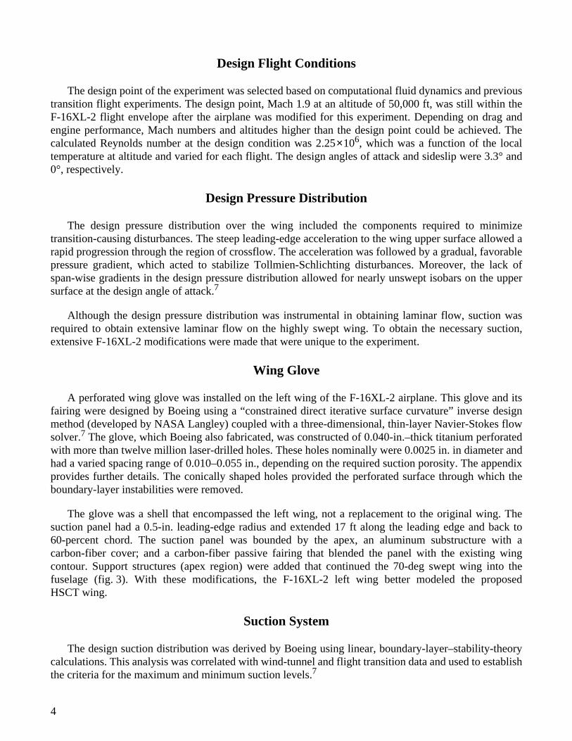
The necessary F-16XL-2 modifications included the installation of a titanium glove on the left wingof the aircraft, the extension of the leading-edge region to continue the 70-deg inboard wing sweep intothe fuselage (fig. 2), and the installation of a suction pump to act as the suction source for the experiment.The objectives of the flight experiment were to achieve 50- to 60-percent–chord laminar flow on a highlyswept wing at supersonic speeds and to validate the tools used in the design of this experiment.

Forty-five flights were conducted at NASA Dryden in support of this experiment. This paperdiscusses research variables that directly impacted the ability to obtain laminar flow and the techniquesused to correct for the variables in flight. These variables included flight conditions, suction, and uniqueF-16XL-2 shock systems.

AIRCRAFT DESCRIPTION

The F-16XL-2 aircraft was selected for this experiment because of its similarity to the proposedHSCT in both its planform (fig. 1) and maximum attainable flight conditions. The F-16XL aircraft has adouble-delta-wing configuration and is a modification of the standard F-16 airplane. The wing leading-edge sweep is 70° and 50° in the inboard and outboard regions, respectively.

The F-16XL-2 airplane was the second F-16 airplane modified by General Dynamics (Fort Worth,Texas). The two-seat aircraft is capable of cruising at Mach 2.0 and an altitude of 55,000 ft whenpowered by the F110-GE-129 engine (General Electric, Evandale, Ohio). Figure 2 shows the left wing ofthe aircraft modified with a laminar flow control glove.

EXPERIMENT DESCRIPTION

Several components, discussed in the following sections, were required to ensure a successfulF-16XL-2 laminar flow experiment. These components included the design flight conditions and pressuredistribution, a wing glove, a suction system, shock fences, a turbulence diverter, and preflight andpostflight monitoring of excrescences.

3

Design Flight Conditions

The design point of the experiment was selected based on computational fluid dynamics and previoustransition flight experiments. The design point, Mach 1.9 at an altitude of 50,000 ft, was still within theF-16XL-2 flight envelope after the airplane was modified for this experiment. Depending on drag andengine performance, Mach numbers and altitudes higher than the design point could be achieved. Thecalculated Reynolds number at the design condition was 2.25×106, which was a function of the localtemperature at altitude and varied for each flight. The design angles of attack and sideslip were 3.3° and0°, respectively.

Design Pressure Distribution

The design pressure distribution over the wing included the components required to minimizetransition-causing disturbances. The steep leading-edge acceleration to the wing upper surface allowed arapid progression through the region of crossflow. The acceleration was followed by a gradual, favorablepressure gradient, which acted to stabilize Tollmien-Schlichting disturbances. Moreover, the lack ofspan-wise gradients in the design pressure distribution allowed for nearly unswept isobars on the uppersurface at the design angle of attack.7

Although the design pressure distribution was instrumental in obtaining laminar flow, suction wasrequired to obtain extensive laminar flow on the highly swept wing. To obtain the necessary suction,extensive F-16XL-2 modifications were made that were unique to the experiment.

Wing Glove

A perforated wing glove was installed on the left wing of the F-16XL-2 airplane. This glove and itsfairing were designed by Boeing using a “constrained direct iterative surface curvature” inverse designmethod (developed by NASA Langley) coupled with a three-dimensional, thin-layer Navier-Stokes flowsolver.7 The glove, which Boeing also fabricated, was constructed of 0.040-in.–thick titanium perforatedwith more than twelve million laser-drilled holes. These holes nominally were 0.0025 in. in diameter andhad a varied spacing range of 0.010–0.055 in., depending on the required suction porosity. The appendixprovides further details. The conically shaped holes provided the perforated surface through which theboundary-layer instabilities were removed.

The glove was a shell that encompassed the left wing, not a replacement to the original wing. Thesuction panel had a 0.5-in. leading-edge radius and extended 17 ft along the leading edge and back to60-percent chord. The suction panel was bounded by the apex, an aluminum substructure with acarbon-fiber cover; and a carbon-fiber passive fairing that blended the panel with the existing wingcontour. Support structures (apex region) were added that continued the 70-deg swept wing into thefuselage (fig. 3). With these modifications, the F-16XL-2 left wing better modeled the proposedHSCT wing.

Suction System

The design suction distribution was derived by Boeing using linear, boundary-layer–stability-theorycalculations. This analysis was correlated with wind-tunnel and flight transition data and used to establishthe criteria for the maximum and minimum suction levels.7

4

A suction control system was designed to achieve the design suction distribution as closely aspossible while applying suction to the panel surface at different levels and locations. Figure 4 shows aschematic of the suction system. Suction was provided for this system by a modified Boeing 707cabin air–pressurization turbocompressor located in the ammunition drum bay. The rate of air drawnthrough the suction-panel holes was measured by mass flow sensors and controlled by butterfly flowcontrol valves (FCVs), which then led into a common chamber, the plenum. From the plenum, air passedthrough a large duct where the master FCV was located. When insufficient quantities of air were drawnthrough the master FCV, a surge valve opened to provide supplemental air to the turbocompressor, whichwas nominally driven by engine-bleed air. All air exiting the turbocompressor was then ventedoverboard, on the right side of the aircraft.

The suction panel was divided into 20 regions, 13 of which were located in the leading edge. Threeflutes, compartments created by fiberglass dividers, provided suction to those regions located in theleading edge. Figure 5 shows the four suction regions fed by each flute. Each of the 20 regions had itsown mass flow sensor and FCV. A setting of 0° represented a closed valve; a setting of 90° represented acompletely open valve.

The suction control system controlled the master FCV and the 20 FCVs through a computer onboardthe aircraft. This computer interfaced in real time the uplinked command signal from the control roomwith the FCVs and set the suction levels for the 20 regions. The FCVs in each region were individuallycontrolled, which allowed for different suction settings within each region. This system permitted severalsuction distributions to be studied during a given flight.

Shock Fences

Because of the engine-inlet configuration of the F-16XL-2 airplane (fig. 6), some concern existed thatinlet-generated shocks could impact the leading edge of the glove, reducing the possibility of obtaininglaminar flow in the affected region. To address this concern, a 20-in.–tall, vertical shock fence wasinstalled on the lower surface of the left wing at butt line (BL) 65. The shock fence was mounted at aweapons ordnance hard-attachment point to block the potential engine-inlet shocks.

Figure 7 shows the two shock-fence designs flown during the experiment. The shock-fence designs,designated by the sweep angle the shock-fence leading edge made with the vertical, were constructed ofaluminum and monitored for strain.8 The first fence flown was the 60-deg shock fence (fig. 7(a)). Thisfence was based on a 10-in.–tall design flown during the previous phase of the F-16XL-2 laminar flowproject.6 The 60-deg shock fence was flown on 19 flights of this experiment. The second fence flown wasthe 10-deg shock fence installed for 24 of the research flights (fig. 7(b)). The 10-deg sweep of this fenceyielded a supersonic leading edge.

Turbulence Diverter

Figure 8 shows a turbulence diverter that was installed inboard of the suction panel at the leadingedge. The turbulence diverter was a passive device used to create a laminar attachment line on the glove.The diverter consisted of a narrow (0.78-in. width) longitudinal slot on the leading edge just inboard ofthe suction panel. This slot allowed the turbulent attachment-line boundary layer flowing outboard fromthe passive-fairing leading edge to be swept away and a new laminar attachment-line boundary layer tobe formed on the inboard leading edge of the panel.

5

Three diverter configurations were flown during the previous phase of the F-16XL-2 laminar flowproject. The design used for this experiment was determined to be the most effective.

Excrescences

Imperfections in the suction panel such as rough spots, dimples, and insect contamination areexamples of the excrescences that can prevent a laminar attachment line. These imperfections can alsocause disturbances in the boundary layer and “trip” the flow downstream of the attachment line fromlaminar to turbulent at the location of the imperfection. Extensive inspections were performed before andafter each flight and detailed records were kept about the locations of any such excrescences. Anomalousbehavior or lack of repeatability in the data occasionally was linked to these excrescences.

Before flight, the suction panel was cleaned thoroughly. Insects primarily were acquired duringtakeoff and landing. The condition of the insect hit allowed for the determination of “insect acquisitiontime” during the flight. Insects acquired during takeoff were particularly difficult to link to anomaliesbecause they could have eroded from the surface during the flight and thus would no longer be presentduring the postlanding inspection. If laminar flow control were used commercially, a shield or some othertype of contamination avoidance system would likely be required to protect the leading edge from insectcontamination during takeoff and landing.9

INSTRUMENTATION

Airdata parameters were measured using a flight test noseboom designed to measure airspeed andflow angles. In addition to the dual flow-angle vanes used to measure the angles of attack and sideslip,the noseboom also provided measurements of total and static pressure. Angle-of-attack calibration datawere obtained during the previous phase of the F-16XL-2 laminar flow experiment. Flow-angleaccuracies were ±0.3° and ±0.5° for the angles of attack and sideslip, respectively.

The aircraft was also instrumented to measure total temperature, Euler angles, accelerations, andcontrol-surface positions. The wing glove instrumentation consisted of pressure orifices, thermocouples,microphones, mass flow sensors, and hot-film anemometers. This paper primarily focuses on the dataobtained from the hot-film anemometers.

Pressure Taps

Figure 9 shows the layout of the pressure taps on the left wing of the F-16XL-2 airplane. Both surfaceand internal pressure measurements were obtained during the experiment. Of the 454 surface pressuretaps, 200 were located on the active suction panel, 113 of which were in the leading-edge region.

The remaining 254 surface pressure taps were located on the passive fairing, including the apexsurrounding the suction panel. These taps were flush-mounted pressure orifices with an internal diameterof 0.0625 in. The 72 internal pressure taps were used to monitor the pressure within the suctionflutes (fig. 9).

6

Mass Flow Sensors

Twenty mass flow sensors were inserted in the ducts between the suction-panel surface and the FCVs.These sensors, designed by Kurz Instruments Inc. (Monterey, California), were used to measure thesuction flow rate in each region. The sensors were based on a Kurz Instruments thermal convectivesingle-point insertion “CD”™ mass velocity sensor and consisted of a glass-coated platinum wire overceramic sealed with epoxy.

The mass flow sensors had an accuracy of ±3 percent of the reading. Each sensor and region valveassembly used to correlate valve position with mass flow was laboratory-calibrated at NASA Langley.

Hot-Film Anemometers

Hot-film sensors with temperature-compensated anemometer systems (fig. 10(a)) were used on oraround the suction panel on both the upper and lower surfaces. Hot-film sensors of this type have beenused on high-performance aircraft in several experiments at NASA Dryden. The sensors were mountedsuch that their active elements were nearly perpendicular to the airflow, with the temperature elementsadjacent and slightly aft of the hot-film sensors to avoid possible flow disturbance over the activeelements of the hot-film sensors. The anemometer system compensates for the local stagnationtemperature, which allows the sensors to operate in conditions where large speed and altitude variationsoccur.10

Twenty-four hot-film sensors were mounted directly to the titanium surface on the edge of the activesuction region on the wing upper surface. The amount of hot films on the active suction surface variedfrom 0 for the first 8 flights to 31 for the final flights (fig. 10(b)). The location of these hot films varied asdifferent areas of the suction panel were investigated. The desire to mount hot films to the active suctionsurface generated some concern about residue blocking the suction-panel holes. As a result, the sensorswere directly mounted not to the surface, but instead to polyester tape that left no residue and was ratedfor high temperatures and dynamic pressures (fig. 10(b)). Before this experiment began, speed andtemperature tests were performed both in flight and in the laboratory to verify that the tape could be usedin this manner.

Although the number of usable lower-surface hot films was limited to 15, the location and number ofthese sensors also varied throughout the flight phase. Initially, 14 lower-surface hot films were used, thefirst of which was mounted to the carbon-fiber panel just forward of the turbulence diverter. The other13 were mounted directly to the titanium surface on the edge of the suction-panel regions. Figure 11shows the 146 hot-film locations studied throughout the flight phase. The number of hot-filmanemometry cards available in the instrumentation system limited the number of recorded hot films to50 preflight-determined hot films.

Data Recording

All instrumentation data were telemetered to the control room in real time during the research flightsand recorded. The airdata and aircraft parameters were measured at 50 samples/sec. The research

7

pressure data were obtained at 12.5 samples/sec. Mass flow data were obtained at 60 samples/sec. Thetelemetered hot-film data were acquired at 100 samples/sec. Hot-film data were also recorded on a14-track magnetic tape drive using frequency modulation and constant bandwidth. These high-frequencydata were recorded at 2 and 10 kHz during the program; however, the results presented in this paper werederived from the telemetered data because transition was easily observed at that frequency. Hot-filmsignals were measured in volts and telemetered to the control room, which allowed decisions regardingflight-maneuver quality to be made in real time.

The hot-film sensor signal used in this experiment had both direct-current (steady-state) andalternating-current (dynamic) components. In previous NASA Dryden experiments, these componentswere separated and recorded as two signals.11 Boundary-layer state classification requires bothcomponents to obtain the best results. For this experiment, the two components were recorded as onesignal.

Figure 12 shows a hot-film signal under a laminar boundary layer that has turbulent bursts boundedby a signal from a turbulent boundary layer at the beginning and the end. The top curve shows thecombined signals; the second curve shows the direct-current (steady-state) component of the signal; andthe bottom curve shows the alternating-current (dynamic) component of the signal. This combinationsignal eliminated some confusion and made boundary-layer state classification an easier process.

Interpretation of Hot-Film Signals

Hot-film sensors were used to determine the boundary-layer state. Figure 13 shows typical hot-filmsignals and their boundary-layer state designation. The dynamic portion of the hot-film signal was“quieter” for laminar flow than for turbulent flow because the temperature-compensated hot-film sensorsrequired less voltage input to keep the temperature constant for laminar flow. Laminar flow required lessvoltage because of little mixing in the boundary layer and therefore less convective heat transfer awayfrom the sensor existed than for turbulent flow. Consequently, the signal had a low amplitude.Conversely, for turbulent flow where heat-transfer rates increase and rapidly fluctuate because of largemixing in the boundary layer, higher voltage was required and the signals had a higher amplitude.

The steady-state portion of the hot-film signal was characterized by a voltage offset. This offset was alower voltage for hot films in areas of laminar flow as opposed to turbulent flow. High-amplitude spikeswere an indication of transitional flow. Spikes in the direction of positive voltage indicated a mostlylaminar signal with turbulent bursts. Spikes in the direction of negative voltage indicated a mostlyturbulent signal with laminar bursts. Peak transition was indicated by a maximum occurrence of high-amplitude spikes.11, 12

TEST CONDITIONS

Data were obtained throughout each research flight; however, the results presented in this paperprimarily were obtained at flight conditions of Mach 2 at altitudes ranging from 50,000 ft to 55,000 ft,angles of attack ranging from 2.0° to 4.0°, and angles of sideslip of either 0.0° or 1.5° nose right. Severaldisturbances occurred, which will be discussed in the “Results” section, that led to the maneuvers

8

primarily being conducted at these flight conditions instead of the design conditions of Mach 1.9, analtitude of 50,000 ft, 3.3° angle of attack, and 0.0° angle of sideslip.

The design conditions were determined from previous flight results and analysis of computationalfluid dynamics results. The desired angles of attack and sideslip were based on the cruise conditions ofthe HSCT (3.5° and 0.0° angles of attack and sideslip, respectively). The maneuvers typically performedwere steady-state pushovers to a predesignated angle of attack. These pushovers were performed withand without sideslip and were approximately 10 sec in duration.

RESULTS

The flight test results presented consist primarily of boundary-layer transition data obtained fromhot-film sensors. In the following sections, pressure distributions, the variables that affect the attachmentline, suction effects, and the extent of laminar flow obtained are discussed.

Shock Fence

Two distinct shocks emanated from the engine inlet. One shock came from the inlet diverter, and theother came from the inlet face (fig. 14(a)). During the previous F-16XL-2 flight tests,6 a 10-in.–tallversion of the 60-deg shock fence was flown to reduce the effect of the inlet-diverter shock on the wingleading edge. Because of the partial effectiveness of that fence, a 20-in.–tall fence was designed for thisexperiment to provide better protection. As will be shown, the 20-in.–tall, 60-deg fence was effective atblocking the inlet-diverter shock, which resulted in a desirable pressure distribution on the leading edge.However, the fence was unable to block the shock off the inlet face, which was further forward(fig.14(a)). This shock was not identified in earlier flight tests because the gloveless wing leading edgewas further inboard and aft.

The sweep angle of the 10-deg shock fence was designed to more effectively block both shockstructures and prevent shock spillage; however, the supersonic leading edge of this fence produced ashock of its own. The resulting expansion altered the leading-edge pressure data, which is exactly whatthe shock fences were designed to prevent. Two flights were flown without either shock fence installed toconfirm the necessity of the shock fence and obtain baseline data.

Pressure Distributions

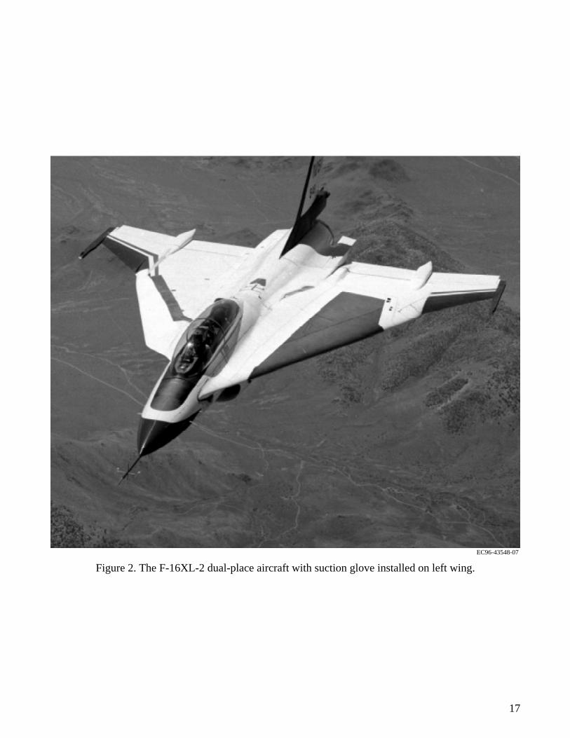
The pressure distribution over the suction glove was measured at constant intervals from BL 50 toBL 110. Several variables influenced the glove pressure distribution, including engine-inlet shock andcanopy-joint shock disturbances (fig. 14). Figure 14(b) shows the canopy-joint shock impingement on theleft wing. Figure 15 shows pressure-distribution data for the suction panel. The data are graphed ascoefficient of pressure ( ) as a function of chord location (x/c) for flight at Mach 2.0.

The open symbols (fig. 15) represent pressure results from flight with the 10-deg shock fenceinstalled. The test condition shown is the maximum laminar flow test point (0.46 x/c), which occurred atan altitude of 53,000 ft, 3.7° angle of attack, and –1.5° angle of sideslip. The solid symbols (fig. 15)represent pressure results from flight with the 60-deg shock fence installed. This test condition resulted in

Cp

9

laminar flow to 0.42 x/c, which occurred at an altitude of 53,000 ft, 3.4° angle of attack, and –1.5° angleof sideslip. This case was the maximum run of laminar flow with the 60-deg shock fence installed. The“X” symbols (fig. 15) represent pressure results for a test point without the shock fence installed, whichoccurred at an altitude of 50,000 ft, 3.7° angle of attack, and 0.0° angle of sideslip. No laminar flow wasachieved during this test condition, and no test points were flown at 53,000 ft without the shock fenceinstalled.

Figure 15 shows pressure-distribution plots for BL 50–100. Both the 10-deg shock-fence data andno shock-fence data were taken at 3.7° angle of attack and generally show good agreement. The 60-degshock-fence data, taken at a slightly reduced 3.4° angle of attack, has slightly higher upper-surfacepressure coefficients. Shock impingement on the glove upper surface was characterized by an adversepressure gradient, indicating increased pressure in the affected region. The engine-inlet shock had a sharppeak because it was a strong shock. The canopy-joint shock was weaker, so the change in the pressurecoefficient was not as large. The circled pressure data (fig. 15) define the locations on the upper surfaceof the suction panel of impingement caused by the two shock-generating systems.

Figures 15(a) and (b) show pressure-distribution data for BL 50 and BL 60. The canopy-joint shock isvisible at BL 60. The lower-surface and leading-edge pressures predictably show excellent agreementbecause these butt lines are inboard of the engine-inlet shock impingement on the leading edge. Thecanopy-joint shock is visible for the data from flight with the 60-deg shock fence installed, but not for theother cases at BL 60. The lack of canopy-joint shock presence at BL 60 is most likely caused by the smallangle-of-attack difference between the test points, which can shift the shock to 0.2 x/c, a location of nopressures.

Figures 15(c) and (d) show the pressure-distribution data for BL 70 and BL 80. Both shock-generatingsystems were identified from data for the three shock-fence configurations. At BL 70, the agreementbetween the 60-deg shock-fence pressure data and data from flight without a shock fence installedindicates the inlet shock was impacting the lower surface. The 10-deg shock-fence data are more negativeat the lower surface, which indicates that the 10-deg fence was better able to block the inlet shock thanthe 60-deg shock fence. The shift in the lower-surface pressures for all three cases indicates the inletshock impinges at the leading edge at BL 80. The canopy-joint shock is also visible for all shock-fenceconfigurations.

Figures 15(e) and (f) show pressure-distribution data for BL 90 and BL 100. The return oflower-surface pressure agreement for all three configurations indicates that the inlet shock impingementaffected the upper surface by lowering the attachment line (that is, lower pressure), and therefore theupper-surface pressures as well. For BL 90 and BL 100, the inlet shock impingement visibly affects theupper-surface pressure data of the flight without a shock fence installed. Canopy-joint shockimpingement occurred on the upper surface for all three shock-fence configurations.

Attachment Line

To achieve laminar flow over a significant portion of the perforated glove, obtaining and maintaininga laminar, leading-edge attachment-line boundary layer on a highly swept wing at supersonic speeds is aprimary concern. Lower-surface hot films placed near the leading edge were used to identify thespan-wise extent of laminar flow at the attachment line.

10

Many variables affect the attachment-line–boundary-layer state. Three of these variables—flightconditions, the shock fences, and the turbulence diverter—contributed to the difficulty in obtaining alaminar attachment line and are discussed in the following subsections.

Flight Condition and Shock-Fence Effects

Key parameters in laminar flow experiments are Reynolds number, angle of attack, and angle ofsideslip. Figures 16–18 show conditions where a laminar attachment line was obtained as a function ofvarious flight parameters. The data were acquired at a Mach range of 1.9–2.0 and an altitude range of50,000–55,000 ft. The symbols (figs. 16–18) represent the test points where all lower-surface hot filmswere laminar, indicating a laminar attachment line. The data are further defined by shock-fenceconfiguration. Triangles represent data from flights when the 60-deg shock fence was installed, andcircles represent the 10-deg shock-fence data. The reason for two shock-fence designs was based on theirinfluence on the attachment line. A completely laminar attachment line was not attainable without ashock fence installed because of the inlet shock effects (discussed in the Shock Fence Resultssubsection). During the two flights without a shock fence installed, 2.9° was the maximum angle ofattack for which the lower-surface hot films inboard of the shock-fence location were laminar. Theoutboard lower-surface hot films were not expected to be laminar because no shock fence was installed tokeep the engine-inlet shock from impacting the attachment line.

Figure 16 shows the data plotted as unit Reynolds number (Re/ft) as a function of angle of attack ( ).The best repeatable laminar flow results achieved at a desirable angle of attack occurred at 3.7° angle ofattack for a unit Reynolds number of 2.23×106/ft. During these research flights, a unit Reynolds numberof 2.23×106/ft was most often attained at Mach 2.0 and an altitude of 53,000 ft. The attachment-linelaminar flow results were very sensitive to angles of attack and sideslip. Investigation with the 10-degshock fence installed proved that a laminar attachment line could be achieved for angles of attack as highas 3.7°. Figure 17 shows angles of attack and sideslip plotted for this test condition. Both positive (noseleft) and negative angles of sideslip were investigated. A laminar attachment line could not be achievedfor positive angles of sideslip. Although a laminar attachment line could be obtained for 0° angle ofsideslip, the most successful laminar flow results repeatedly were obtained by “unsweeping” the left wingto –1.5° angle of sideslip (fig. 18).

Turbulence Diverter Effects

Preflight predictions indicated local upper-surface streamlines such that turbulent wedges from theinboard row of hot films would not contaminate hot films downstream. However, the inboard region ofthe suction-panel upper surface (fig. 11) was always turbulent. This turbulent boundary layer waspostulated to have been formed because the turbulence diverter was not removing all of the oncomingturbulent flow, thus preventing a laminar boundary layer from being formed in the inboard suction-panelregions. Moreover, the turbulence diverter may also have been generating a vortex that would causeturbulent flow along the inboard edge of the glove.

To verify this theory, the turbulence diverter was filled with low-density foam and room-temperaturevulcanizing silicon 4130, and coated with epoxy (fig. 19). When filled, the turbulence diverter was nolonger able to remove the turbulent boundary layer to allow a laminar attachment line to form. Instead,the attachment line was completely turbulent, regardless of suction distributions or flight conditions. Thehypothesis then was that both the turbulence diverter and the canopy-joint shock were the cause of the

α

11

turbulent inboard upper-surface region. The forward portion of the turbulent inboard region was mostlikely caused by a vortex generated by the turbulence diverter. The aft portion of the turbulent inboardregion was a high-crossflow region caused by the shock off the canopy joint discussed in the PressureDistribution Results subsection.7

Suction Effects on Transition

To achieve laminar flow, the experiment used FCVs in the ducts to actively control suction on theperforated suction glove. Obtaining the optimum suction distribution over the panel was extremelyimportant and challenging. Figure 20 shows the design suction distribution at Mach 1.9 and an altitudeof 50,000 ft. Figure 20 also shows a flight suction distribution that repeatedly yielded successful laminarflow results at Mach 2.0 and an altitude of 55,000 ft. The flight suction values in flute 1 represent thelaminar attachment-line, flight-determined optimum suction level. A laminar attachment line could notbe obtained for suction coefficient values in excess of these values, which were usually less than designin the attachment-line regions.

Evidence that the design levels may have been too high in the attachment-line regions was obtainedwhen the suction system was turned off. Because the suction system usually was not turned on until theaircraft was nearing the flight test conditions, time existed to observe the behavior of the hot films withthe suction off. The lower-surface hot films located span-wise between the turbulence diverter and theshock fence were often laminar without suction at altitudes and Mach numbers ranging from 45,000 to50,000 ft and 1.69 to 1.93, respectively. Figure 21 shows examples of this phenomenon. These sensorsbecame turbulent when design suction was turned on because of too much suction in the attachment-lineregions. However, preflight predictions had shown the design suction level necessary to overcome theleading-edge pressure disturbance from the inlet shock. This need for lower-than-design suction occurredonly on the attachment line; hot films in the other suction regions could be laminar with design suction.In fact, suction in the remaining leading-edge regions was set at levels higher than design (fig. 20) tocompensate for the limited levels in the attachment-line regions.7

Figures 22–26 show examples of the effectiveness of these and other suction settings in flight at aspeed of Mach 2.0 and altitudes ranging from 53,000 to 55,000 ft. The data are from the wing glove withthe 10-deg shock fence installed and from hot-film sensors indicating the boundary-layer state for aspecific suction distribution. The comparison plots (figs. 22–26) were compiled from several flights, andthe hot-film layout varied from flight to flight. The boundary-layer state in a specific region varied assuction changed within that region.

In the attachment-line regions, the FCVs were all set to the same flight values as those shown infigure 20, with some variation for region 11. Any disparity in the mass flow (that is, the suctioncoefficient) for constant valve settings were caused by changes in flight condition. Throughout the flightexperiment, the suction valve in region 20 was closed and no hot films were placed on the suction-panelsurface in that area, because laminar flow was not expected to be seen. Note that, when shown, the upper-surface hot films inboard of the suction-panel regions are always turbulent, as mentioned in theTurbulence Diverter Effects Results subsection.

Figure 22 shows three cases that demonstrate the effect of glove suction variation on thelower-surface hot films (that is, the attachment-line–boundary-layer state). In these cases, suction

12

variations occur in all regions except regions 1, 2, 5, and 8, located at the attachment line. The variationsin region 11, also located at the attachment line, indicate that the three hot films furthest aft on the lowersurface (closest to region 11) were affected. Although the suction in region 11 (figs. 22(a) and (b)) wasessentially the same, the turbulent-with-laminar-bursts signal on the outboard leading edge (fig. 22(a))occurred because the suction in flutes 2 and 3 was not enough, as compared to that in figure 22(b), tosustain the laminar flow conditions on the panel. Figure 22(b) shows the effectiveness of maximumsuction in the leading-edge regions, (that is, the FCVs in those regions were open the maximumamount, 90°). Decreasing the suction in region 11 finally produced the desired laminar attachment line(fig. 22(c)).

Figure 23 shows two suction distributions. The suction in the leading-edge regions was identical inboth cases, and the lower-surface hot films indicated the same boundary-layer state for the attachmentline in both test points. Figure 23 shows a comparison of the upper-surface suction settings thatdemonstrate the necessity of higher suction in regions 14–19. The upper-surface boundary-layer state(fig. 23(a)) was mostly turbulent with laminar bursts. Increasing the rooftop suction produced thelaminar-with-turbulent-spikes signal on the upper-surface hot films (fig. 23(b)).

Figure 24 shows a good example of attachment-line and boundary-layer state repeatability. As infigure 23, suction variations occurred only in the rooftop regions. As expected, the lower-surface hot filmsignals were identical for both cases. The suction settings in the rooftop regions further demonstrate thenecessity for higher suction in those areas in order to obtain laminar flow over a large percentage of theglove.

Figure 25 shows an indication of the lack of sensitivity of the upper-surface boundary-layer state tosmall variations in suction. The suction settings in the leading-edge regions were the same as in figure 24,with variation only in regions 14–19. The valves in the upper-surface regions varied from 40° (fig. 25(a))to 45° (fig. 25(b)). The hot-film states were very similar to those in figure 24. By using a multiple-regionsuction coefficient ( ), a 13.7-percent difference exists with ±3.7-percent error in the suction

distribution for regions 14–19 of the two cases. Therefore, when the suction in the leading-edge regionswas held constant, the boundary layer was not very sensitive to small changes in rooftop suction. Thisinsensitivity is further demonstrated by a comparison of figure 25(b) with figure 24(b). A 10.7-percent

difference exists with ±3.7-percent error in the suction distribution for regions 14–19 and very

little variation exists in the hot-film signals.

The leading-edge suction values (fig. 26) represent the flight-determined optimum suction settings fora laminar attachment line. The large steps in suction in the rooftop regions (figs. 26(a)–(c)) demonstratethe necessity for high suction in these regions. The small FCV angles (fig. 26(a)) yielded mostly turbulenthot-film signals, but the hot films in figure 26(b) indicate more laminar signals for a 20-deg change inFCV position. The suction distribution shown in figure 26(c) is the same flight distribution shown infigure 20; valves in the rooftop regions are open to 90°. This distribution also yielded a laminarattachment line and laminar flow in the rooftop regions. The turbulent and turbulent-with-laminar-burstssignals in region 15 were caused by the existence of the hot-film sensors mounted forward of the sensorsin region 14.

CqMR

CqMR

13

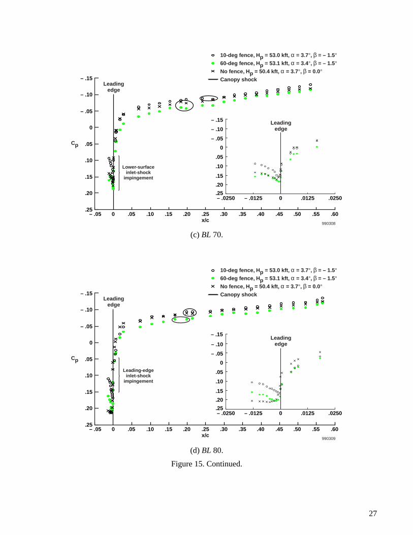
Extent of Laminar Flow

When all of the attachment-line variables were taken into account and the suction system had beenexercised and its limits understood, the extent of laminar flow could be maximized. Figures 27 and 28show two cases that document the long runs of laminar flow achieved at Mach 2 during the course of theprogram. The figures show the wing glove with hot-film sensors that indicate the state of the boundarylayer for a specific suction distribution. The shaded area represents the region of laminar flow over thewing glove. In both cases, all the lower-surface hot films were laminar, indicating a laminar attachmentline. The suction distribution for each case, including the design suction, is also shown. As in thedistribution from figures 20 and 26(c), maximum suction was employed in flutes 2 and 3 and in therooftop regions, with suction variation occurring only for the attachment-line regions. A 45.3-percent

difference exists with ±3.3 percent error between the flute 1 suction distributions of the two cases.

Both of the cases shown were obtained with the 10-deg shock fence installed.

In figure 27, the laminar flow region is bounded by turbulent and laminar-with-turbulent-burstshot-film signals. The hot film furthest aft to indicate laminar flow for this test point was located at0.41 x/c, which made the maximum laminar flow distance a minimum of 8.60 ft. This locationcorresponds to a Reynolds number of 21.2×106 at 2.6° angle of attack and 0.0° angle of sideslip. Theattachment-line suction distribution was not the flight-determined optimum discussed in the SuctionEffects on Transition Results subsection. However, a laminar attachment line was still attainable becauseof the low angle of attack, which was lower than the desired HSCT cruise angle of attack.

Figure 28 shows the laminar flow region bounded by turbulent and transitional hot-film signals. Thistest point occurred at 3.7° angle of attack (closer to the desired HSCT cruise angle of attack than those offigure 27), –1.5° angle of sideslip, and a Reynolds number of 22.7×106. The hot film furthest aft to belaminar was located at 0.46 x/c, which made the laminar flow distance 10.30 ft. Except for the very smallvariation in region 11, the suction distribution shown is identical to those shown in figures 20 and 26(c).

These long runs of laminar flow were not the only cases. In fact, a very good example of repeatabilityoccurred on the last flight where 14 test points consistently demonstrated laminar flow as far aft as0.42 x/c. All of these cases occurred at Mach 2.0 and an altitude of 53,000 ft; used the attachment-lineflight-determined optimum suction levels; and had variation occur only in flutes 2 and 3 and in therooftop regions. Unfortunately, the direct-current level of several hot-film sensors was out of range onthat flight, so the actual extent of laminar flow was unknown.

CONCLUDING REMARKS

A titanium, laminar flow control glove with variable hole spacing has been flown on the left wing ofthe F-16XL-2 aircraft. Boundary-layer transition data have been obtained on this glove primarily atMach 2.0 and altitudes of 53,000 to 55,000 ft.

Best results have been obtained at Mach 2.0 and an altitude of 53,000 ft rather than the design Machnumber and altitude (Mach 1.9 and 50,000 ft, respectively). At an angle of attack (3.7°) near the desiredcruise angle for the High-Speed Civil Transport (HSCT), laminar flow was obtained to a minimum0.46 chord location (x/c) corresponding to a Reynolds number of 22.7×106. Laminar flow has beenconsistently obtained to a minimum 0.42 x/c with the flight-determined optimum suction levels.

CqMR

14

Reducing suction levels at the attachment line from the design levels was necessary to obtain alaminar attachment line. However, increasing the suction levels above design on the rest of the panel wasrequired to maximize the laminar flow conditions further aft.

Shocks peculiar to the F-16XL-2 airplane caused some compromises in the experiment. Shocks offthe inlet required a shock fence to be installed on the lower surface of the left wing and the airplane to beflown at an angle of sideslip of 1.5° nose right. At times, a shock off the canopy joint resulted inunfavorable pressure gradients and boundary-layer transition on the upper surface. These shocks andresulting effects would not be present on a HSCT implementing laminar flow control technology.

15

EC91 0646-01

(a) The F-16XL-2 airplane.

EL-1998-00001

(b) HSCT concept.

Figure 1. Comparison of the unmodified F-16XL-2 and HSCT aircraft.

16

EC96-43548-07

Figure 2. The F-16XL-2 dual-place aircraft with suction glove installed on left wing.

17

Figure 3. Aircraft configuration.

Figure 4. Suction system schematic.

Active suction glove

Passive fairing

Apex region

Passive glove (previous experiment)

15.68 ft 6.54 ft

3.19 ft

70°5°

5°

Shock fence (lower surface)

990291

990292

Turbocompressor

Manifold

Engine- bleed air

Supplementalair

Ventedoverboard

on the rightside of the

aircraft

Master FCV

Suction panel

FCV(s)

Mass flowsensor(s)

Surgevalve

18

Figure 5. Suction-panel regions.

Figure 6. The F-16XL-2 engine inlet.

Leading-edge regions (not to scale)

20

1918

1615

141

2, 3, 4

5, 6, 7

8, 9, 10

11, 12, 13

17

13

4

6

7

9

10

12

13

2 5 8 11

Leading-edge regions

Side view(not to scale)

Flute 2

Flute 1

Flute 3

Suction panelShock fence (lower surface)

Leadingedge

990293

990294

Inlet diverter

19

(a) 60-deg shock fence.

(b) 10-deg shock fence.

Figure 7. Shock-fence configurations.

990295

60°

Strain gages

990296

10°

Strain gages

20

Figure 8. Turbulence diverter.

Figure 9. Suction-panel and passive-fairing pressure tap layout.

990297

Carbon-fiber panel

Titanium glove

Turbulence diverter Width = 0.78 in. along leading edge

Suction-panel pressure taps (200)

Passive-fairing pressure taps (254)

Internal flute pressure taps (72)Passive fairing


990298

21

(a) Hot film.

(b) Upper-surface hot films.

Figure 10. Hot-film anemometers.

Temperature sensor

Hot-film sensor

Air flow

990299Active element

Bla

ck

Sh

ield

Wh

ite

990300

Air flow

Suction-panel–edge hot films

22

Figure 11. Hot-film locations studied.

990301

Upper-surface hot films on suction-panel surface = 102Upper-surface hot films on suction-panel edge = 24Lower-surface hot films = 20Total number of hot-film locations = 146

Leading edge

Leading edge

Suction-panel inboard edge

Hot-film sensorSuction region boundarySuction-panel boundaryTitanium panel edge


23

Figure 12. Hot-film signal components.

Figure 13. Hot-film signal classification.

Laminar-with-turbulent-bursts signal

Time, sec990302

– 2

0

2Dynamic alternating-current component

V

– 2

0

2

V

– 2

0

2

V

Steady-state direct-current component

T LT T

T LT T

TLT

T

T

– 2

0

2

LTT

T

T

T

T

TR T

TL T

T

Time, sec

V

– 2

0

2

V

– 2

0

2

V

– 2

0

2

V

– 2

0

2

VL

990303

24

(a) Lower surface.

(b) Upper surface.

Figure 14. Shock disturbances.

Inlet diverter

Shock fence

Inlet-shock systems

990304

Canopy-joint shock

BL 50BL 60

BL 70BL 80

BL 90

BL 110

990305

BL 100

Suction-panel pressure taps

25

(a) BL 50.

(b) BL 60.

Figure 15. Pressure distributions for Mach 2.0.

990306

Cp

10-deg fence, Hp = 53.0 kft, α = 3.7°, β = – 1.5°60-deg fence, Hp = 53.1 kft, α = 3.4°, β = – 1.5°No fence, Hp = 50.4 kft, α = 3.7°, β = 0.0°Canopy shock– .15

– .10

– .05

0

.05

.10

.15

.20

.25

– .15

– .10

– .05

0

.05

.10

.15

.20

.25

– .05 0 .05 .10 .15 .20 .25x/c

.30 .35 .40 .45 .50 .55 .60

Leadingedge

Leadingedge

– .0250 – .0125 0 .0250.0125

990307

Cp

– .15

– .10

– .05

0

.05

.10

.15

.20

.25

– .15

– .10

– .05

0

.05

.10

.15

.20

.25

– .05 0 .05 .10 .15 .20 .25x/c

.30 .35 .40 .45 .50 .55 .60

Leadingedge

Leadingedge

– .0250 – .0125 0 .0250.0125

10-deg fence, Hp = 53.0 kft, α = 3.7°, β = – 1.5°60-deg fence, Hp = 53.1 kft, α = 3.4°, β = – 1.5°No fence, Hp = 50.4 kft, α = 3.7°, β = 0.0°Canopy shock

26

(c) BL 70.

(d) BL 80.

Figure 15. Continued.

990308

Cp

– .15

– .10

– .05

0

.05

.10

.15

.20

.25

– .15

– .10

– .05

0

.05

.10

.15

.20

.25

– .05 0 .05 .10 .15 .20 .25x/c

.30 .35 .40 .45 .50 .55 .60

Leadingedge

Leadingedge

– .0250 – .0125 0 .0125 .0250

Lower-surfaceinlet-shock

impingement


990309

Cp

– .15

– .10

– .05

0

.05

.10

.15

.20

.25

– .10

– .05

0

.05

.10

.15

.20

.25

– .05 0 .05 .10 .15 .20 .25x/c

.30 .35 .40 .45 .50 .55 .60

Leadingedge

Leadingedge

– .0250 – .0125 0 .0125 .0250

Leading-edgeinlet-shock

impingement

– .15


27

(e) BL 90.

(f) BL 100.

Figure 15. Concluded.

990310

Cp

– .15

– .10

– .05

0

.05

.10

.15

.20

.25

– .10

– .05

0

.05

.10

.15

.20

.25

– .05 0 .05 .10 .15 .20 .25x/c

.30 .35 .40 .45 .50 .55 .60

Leadingedge

Leadingedge

– .0250 – .0125 0 .0125 .0250

– .15

10-deg fence, Hp = 53.0 kft, α = 3.7°, β = – 1.5°60-deg fence, Hp = 53.1 kft, α = 3.4°, β = – 1.5°No fence, Hp = 50.4 kft, α = 3.7°, β = 0.0°Canopy shockInlet shock

990311

Cp

– .15

– .10

– .05

0

.05

.10

.15

.20

.25

– .10

– .05

0

.05

.10

.15

.20

.25

– .05 0 .05 .10 .15 .20 .25x/c

.30 .35 .40 .45 .50 .55 .60

Leadingedge

Leadingedge

– .0250 – .0125 0 .0125 .0250

– .15

10-deg fence, Hp = 53.0 kft, α = 3.7°, β = – 1.5°60-deg fence, Hp = 53.1 kft, α = 3.4°, β = – 1.5°No fence, Hp = 50.4 kft, α = 3.7°, β = 0.0°Canopy shockInlet shock

28

Figure 16. Reynolds number and angle-of-attack test conditions under which a laminar attachment linewas obtained.

Figure 17. Angle-of-attack and -sideslip test conditions under which a laminar attachment line wasobtained.

2.0

1.5 2.0 2.5 α, deg

3.0 3.5 4.0

2.5

3.0 x 106

Re/ft

990312

10-deg shock fence 60-deg shock fenceM = 1.9 – 2.0Hp = 50.2 – 55.4 kft

α = 2.0°– 3.7°β = – 1.6°– 0.1°

2.0

1.5– 1.5– 2.0 – 1.0

β, deg– .5 0 .5

2.5

3.0

3.5

4.0

α,deg

990313


α = 2.0°– 3.7°β = – 1.6°– 0.1°

29

Figure 18. Reynolds number and angle-of-sideslip test conditions under which laminar attachment linewas obtained.

2.0

1.5– 1.5– 2.0 – 1.0

α, deg– .5 0 .5

2.5

3.0 x 106

Re/ft

990314

See below


α = 2.0°– 3.7°β = – 1.6°– 0.1°

2.0

2.1

2.2

2.3

– 1.6– 1.6 – 1.5 α, deg

– 1.5 – 1.4 – 1.4

2.4 x 106

Re/ft

990315


α = 2.0°– 3.7°β = – 1.6°– 0.1°

30

(a) Nominal.

(b) Filled.

Figure 19. Turbulence diverter.

990316

Turbulence diverter

990317

Turbulence diverter filled

31

Figure 20. Suction distribution.

Figure 21. Lower-surface hot films without suction.

0

– 0.0005

– 0.0010

– 0.0015

– 0.0020

– 0.0025

1 2 5 8 11 3 6 9 12 4 7 10 13 14 15 16 17 18 19 20Flute 1 Flute 2 Flute 3 Rooftop

} Regions

990318

Attachment Line

Leading edge

Flight: M = 2.0; Hp = 55 kft

Design: M = 1.9; Hp = 50 kft

Cq

Region 2 Region 5

LSHF02 LSHF03 LSHF04 LSHF05 LSHF06 LSHF07 LSHF08

Spanwise distance

FSBL

20°

Shock fence

990319

Leadingedge

Lower surface hot films

M

1.690

1.807

1.861

1.898

1.901

1.933

Hp, kft

50.5

50.7

50.4

49.7

45.1

50.7

Re, mil/ft

1.97

2.12

2.20

2.42

2.81

2.26

α, deg

4.24

3.96

3.96

3.24

3.13

3.95

2

L

L

LT

LT

L

L

5

L

L

LT

LT

LT

LT

6

T

T

L

L

L

T

7

T

T

T

T

T

T

8

T

T

T

T

T

T

3

L

L

L

L

L

L

4

L

L

L

L

L

L

32

(a) FCV angles: region 11 = 40°; flutes 2 and 3 = 37°; regions 14–19 = 37°.

(b) FCV angles: region 11 = 40°; flutes 2 and 3 = 90°; regions 14–19 = 35°.

Figure 22. Suction effects at Mach 2.0, an altitude of 53,200 ft, 3.7° angle of attack, and –1.5° angle ofsideslip.

990320

– .0020

– .0015

– .0010

– .0005

01 2 3 4 5 6 7 8 9 10

Region11 12 13 14 15 16 17 18 19 20

Cq

Lower-surface hot film

14

15

16

1718 19

2010-deg shock fence

Suction-panel edge

Hot-filmsensor states

LLTTRTLT

990321

– .0020

– .0015

– .0010

– .0005

01 2 3 4 5 6 7 8 9 10

Region11 12 13 14 15 16 17 18 19 20

Cq


10-deg shock fence

Suction-panel edge

14

15

16

1718 19

20


LLTTRTLT

33

(c) FCV angles: region 11 = 30°; flutes 2 and 3 = 90°; regions 14–19 = 90°.


990322

– .0020

– .0015

– .0010

– .0005

01 2 3 4 5 6 7 8 9 10

Region11 12 13 14 15 16 17 18 19 20

Cq


10-deg shock fence

Suction-panel edge

14

15

16

1718 19

20


LLTTRTLT

34

(a) Regions 14–19 FCV angles = 17.5°.

(b) Regions 14–19 FCV angles = 90°.

Figure 23. Rooftop suction effects at Mach 2.0, an altitude of 53,300 ft, 3.7° angle of attack, and –1.4°angle of sideslip.

990323

– .0020

– .0015

– .0010

– .0005

01 2 3 4 5 6 7 8 9 10

Region11 12 13 14 15 16 17 18 19 20

Cq


10-deg shock fence

Suction-panel edge

14

15

16

1718 19

20


LLTTRTLT

990324

– .0020

– .0015

– .0010

– .0005

01 2 3 4 5 6 7 8 9 10

Region11 12 13 14 15 16 17 18 19 20

Cq


10-deg shock fence

Suction-panel edge

14

15

16

1718 19

20


LLTTRTLT

35

(a) Regions 14–19 FCV angles = 20°.



990325

– .0020

– .0015

– .0010

– .0005

01 2 3 4 5 6 7 8 9 10

Region11 12 13 14 15 16 17 18 19 20

Cq


10-deg shock fence

Suction-panel edge 14

15

1617

18

19

20


LLTTRTLT

990326

– .0020

– .0015

– .0010

– .0005

01 2 3 4 5 6 7 8 9 10

Region11 12 13 14 15 16 17 18 19 20

Cq


10-deg shock fence


15

1617

18

19

20


LLTTRTLT

36




990327

– .0020

– .0015

– .0010

– .0005

01 2 3 4 5 6 7 8 9 10

Region11 12 13 14 15 16 17 18 19 20

Cq


10-deg shock fence


15

16 1718

19

20


LLTTRTLT

990328

– .0020

– .0015

– .0010

– .0005

01 2 3 4 5 6 7 8 9 10

Region11 12 13 14 15 16 17 18 19 20

Cq


10-deg shock fence


15

16 1718

19

20


LLTTRTLT

37




990329

– .0020

– .0015

– .0010

– .0005

01 2 3 4 5 6 7 8 9 10

Region11 12 13 14 15 16 17 18 19 20

Cq


10-deg shock fence


15

16 1718

19

20


LLTTRTLT

990330

– .0020

– .0015

– .0010

– .0005

01 2 3 4 5 6 7 8 9 10

Region11 12 13 14 15 16 17 18 19 20

Cq


10-deg shock fence


15

16 1718

19

20


LLTTRTLT

38

(c) Regions 14–19 FCV angles = 90°.


990331

– .0020

– .0015

– .0010

– .0005

01 2 3 4 5 6 7 8 9 10

Region11 12 13 14 15 16 17 18 19 20

Cq


10-deg shock fence


LLTTRTLT


15

16 1718

19

20

39

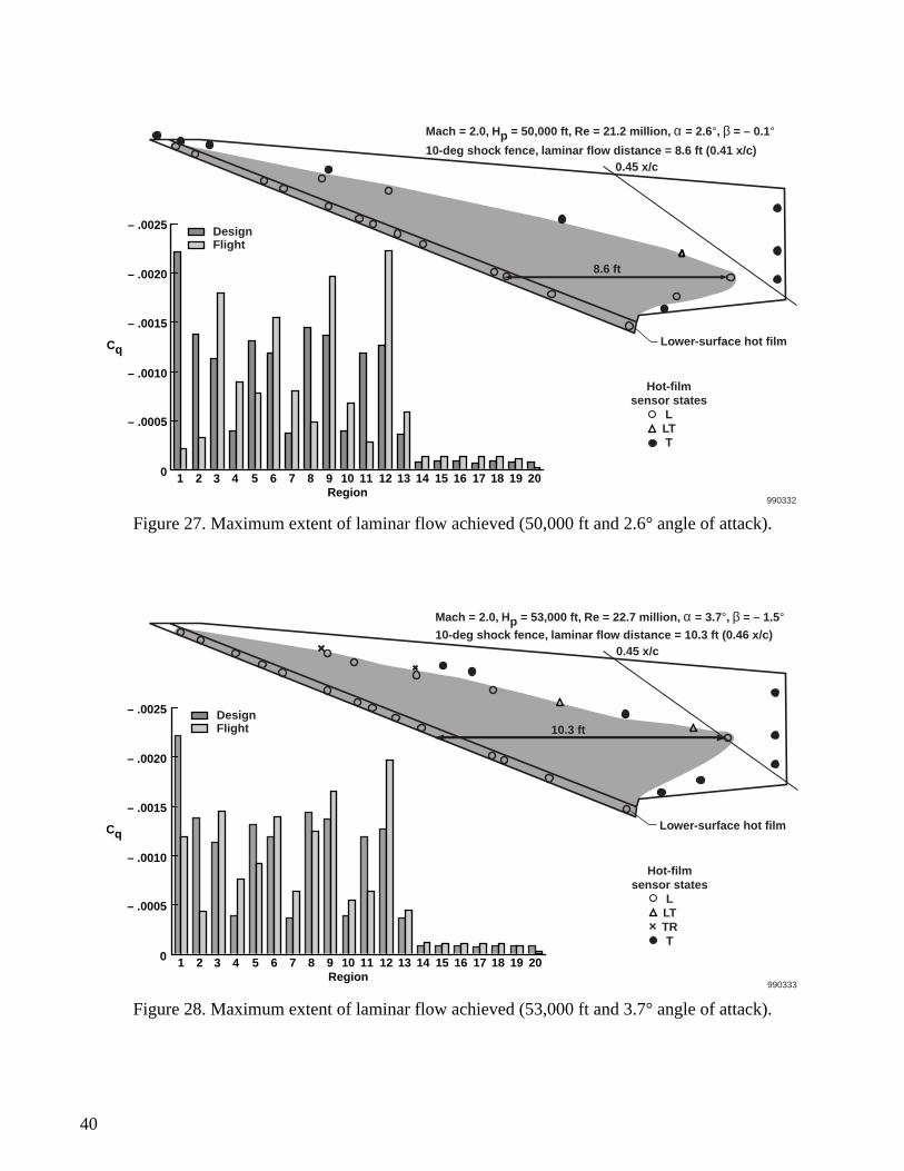
Figure 27. Maximum extent of laminar flow achieved (50,000 ft and 2.6° angle of attack).

Figure 28. Maximum extent of laminar flow achieved (53,000 ft and 3.7° angle of attack).

990332

– .0020

– .0025

– .0015

– .0010

– .0005

0 1 2 3 4 5 6 7 8 9 10Region

11 12 13 14 15 16 17 18 19 20

CqLower-surface hot film

Hot-film

sensor statesLLTT

Mach = 2.0, Hp = 50,000 ft, Re = 21.2 million, α = 2.6°, β = – 0.1°10-deg shock fence, laminar flow distance = 8.6 ft (0.41 x/c)

FlightDesign

0.45 x/c

8.6 ft

990333

– .0020

– .0025

– .0015

– .0010

– .0005

0 1 2 3 4 5 6 7 8 9 10Region

11 12 13 14 15 16 17 18 19 20

CqLower-surface hot film


LLTTRT

Mach = 2.0, Hp = 53,000 ft, Re = 22.7 million, α = 3.7°, β = – 1.5°10-deg shock fence, laminar flow distance = 10.3 ft (0.46 x/c)

10.3 ftFlightDesign

0.45 x/c

40

APPENDIX

Laminar Flow Control Suction Panel Description

The variable-porosity (hole spacing) suction panel installed on the left wing of the F-16XL-2 airplanewas composed of more than twelve million laser-drilled holes of 0.0025-in. constant diameter. The holespacing, however, equally varied (in rows and columns) from 0.010 to 0.055 in. The titanium panel wasdivided into 20 regions (fig. 5), each with variable porosity designed to provide within ±5 percent of thedesign suction level in each region. These regions were further divided into patches that were defined byconstant porosity. Table A-1 shows the regions, patches, and hole spacing.

Figures A-1–A-12 show the individual regions, patches, and hole spacing of the suction panel indetail. The numbers within a region represent the patch numbers listed in table A-1. This numbering isconsecutive in regions 1–13. In these figures, double lines surround regions and dashed lines surroundpatches. The aluminum stringers that separated the upper and lower titanium skin are depicted by therectangles with hatched lines. The large hatched band in regions 15–19 represents the splice joint wheretwo pieces of titanium were joined together to create the suction panel. Suction holes were blocked (thatis, no suction existed) wherever hatched lines are shown.

41

Table A-1. Suction glove hole spacing.

Patchnumber

Regionnumber

Holespacing, in.

Patchnumber

Regionnumber

Holespacing, in.

Patchnumber

Regionnumber

Holespacing, in.

1

1

0.017 48

9

0.014 95.1 16 0.031

2 0.010 49 0.014 95.2 17 0.031

3 0.012 50 0.014 96.1 16 0.031

4 0.017 51

10

0.017 96.2 17 0.031

5

2

0.017 52 0.023 97.1 16 0.031

6 0.016 53 0.033 97.2

17

0.031

7 0.016 54 0.048 98 0.025

8

3

0.016 55

8

0.016 99 0.024

9 0.016 56 0.015 100 0.025

10 0.016 57 0.014 101

18

0.028

11

4

0.019 58

9

0.014 102 0.028

12 0.023 59 0.014 103 0.028

13 0.034 60 0.014 104 0.028

14 0.050 61

10

0.016 105 0.027

15

2

0.017 62 0.019 106 19 0.030

16 0.016 63 0.023 10715

0.035

17 0.015 64 0.032 108 0.031

18

3

0.015 65

11

0.015 109

16

0.033

19 0.014 66 0.014 110 0.033

20 0.014 67 0.013 111.1 0.031

21

4

0.019 68

12

0.013 111.2

17

0.031

22 0.023 69 0.012 112 0.025

23 0.033 70 0.012 113 0.024

24 0.050 71

13

0.016 114

18

0.028

25

5

0.017 72 0.018 115 0.028

26 0.016 73 0.027 116 0.027

27 0.015 74 0.045 117 0.027

28

6

0.017 75

11

0.015 118 0.027

29 0.017 76 0.014 119

19

0.030

30 0.017 77 0.013 120 0.028

31

7

0.018 78

12

0.013 121 0.024

32 0.024 79 0.012 122 0.023

33 0.034 80 0.012 123 20 0.015

34 0.050 81

13

0.016

35

5

0.016 82 0.016

36 0.015 83 0.024

37 0.014 84 0.040

38

6

0.015 85

14

0.055

39 0.015 86 0.051

40 0.015 87 0.044

41

7

0.016 88 0.045

42 0.019 89 0.032

43 0.032 90 0.031

44 0.045 9115

0.035

45

8

0.016 92 0.031

46 0.015 9316

0.033

47 0.014 94 0.033

42

Figure A-1. Suction-panel region 1.

Figure A-2. Suction-panel regions 2–4.


1

3

4

RegionPatch

Suction boundary legend

2

Leadingedge

990334

Region 4

Region 3

Region 2


990335

Stringer

Region

Patch

579

11121314

151719

21222324


990336

Stringer

Region

Patch

Region 7

Region 6

Region 525272931323334

35373941424344

43





990337

Stringer

Region

Patch

Region 10

Region 9

Region 845474951525354

55575961626364


990338

Stringer

Region

Patch

Region 13

Region 12

Region 1165676971727374

75777981828384

990339

Stringer

Region

Patch


85

8687

88

90

89

44



91

107108

92

990340

Splice joint

Stringer

Region

Patch


95.1

96.1

97.1

109

110 111.1

93

94

990341

Splice joint

Stringer

Region

Patch


45



95.2

96.2

97.2

112

113

111.2

99

98

100

990342

Splice joint

Stringer

Region

Patch


101

102

103

117

115118

114

105

104

116

990343

Splice joint

Stringer

Region

Patch


46



106

120122

121119

990344

Splice joint

Stringer

Region

Patch


123

990345

Stringer

Region

Patch


47

REFERENCES

1. Powell, A. G., S. Agrawal, and T. R. Lacey, Feasibility and Benefits of Laminar Flow Control onSupersonic Cruise Airplanes, NASA CR-181817, 1989.

2. Boeing Commercial Airplane Company, Application of Laminar Flow Control to SupersonicTransport Configurations, NASA CR-181917, 1990.

3. Pfenninger, Werner and Chandra S. Vemuru, “Design Aspects of Long Range Supersonic LFCAirplanes with Highly Swept Wings,” SAE-881397, Oct. 1988.

4. Anderson, Bianca T. and Marta Bohn-Meyer, Overview of Supersonic Laminar Flow ControlResearch on the F-16XL Ships 1 and 2, NASA TM-104257, 1992.

5. Anderson, Bianca T., Bruce H. Rowan, and Stephen F. Landers, F-16XL Supersonic Laminar FlowControl Glove Initial Flight Test Results, NASA TM-104270, 1993.

6. Landers, Stephen F., John A. Saltzman, and Lisa J. Bjarke, F-16XL Wing Pressure Distributions andShock Fence Results from Mach 1.4 to Mach 2.0, NASA TM-97-206219, 1997.

7. Anders, Scott G. and Michael C. Fischer, F-16XL-2 Supersonic Laminar Flow Control Flight TestExperiment, NASA TP-1999-209683, 1999.

8. Olney, Candida D. and Joseph V. Collura, A Limited In-Flight Evaluation of the Constant CurrentLoop Strain Measurement Method, NASA TM-104331, 1997.

9. Wagner, R. D., D. V. Maddalon, and D. F. Fisher, “Laminar Flow Control Leading Edge Systems inSimulated Airline Service,” presented at the 16th Congress of the International Council of theAeronautical Sciences, Jerusalem, Israel, August 28–September 2, 1988.

10. Chiles, Harry R., The Design and Use of a Temperature-Compensated Hot-Film Anemometer Systemfor Boundary-Layer Flow Transition Detection on Supersonic Aircraft, NASA TM-100421, 1988.

11. Anderson, Bianca Trujillo, Robert R. Meyer, Jr., and Harry R. Chiles, Techniques Used in the F-14Variable-Sweep Transition Flight Experiment, NASA TM-100444, 1988.

12. Obara, Clifford J. and Bruce J. Holmes, Flight-Measured Laminar Boundary-Layer TransitionPhenomena Including Stability Theory Analysis, NASA TP-2417, 1985.

48

REPORT DOCUMENTATION PAGE Form ApprovedOMB No. 0704-0188

Public reporting burden for this collection of information is estimated to average 1 hour per response, including the time for reviewing instructions, searching existing data sources, gathering andmaintaining the data needed, and completing and reviewing the collection of information. Send comments regarding this burden estimate or any other aspect of this collection of information,including suggestions for reducing this burden, to Washington Headquarters Services, Directorate for Information Operations and Reports, 1215 Jefferson Davis Highway, Suite 1204, Arlington,VA 22202-4302, and to the Office of Management and Budget, Paperwork Reduction Project (0704-0188), Washington, DC 20503.

1. AGENCY USE ONLY (Leave blank) 2. REPORT DATE 3. REPORT TYPE AND DATES COVERED

4. TITLE AND SUBTITLE 5. FUNDING NUMBERS

6. AUTHOR(S)

8. PERFORMING ORGANIZATION REPORT NUMBER

7. PERFORMING ORGANIZATION NAME(S) AND ADDRESS(ES)

9. SPONSORING/MONITORING AGENCY NAME(S) AND ADDRESS(ES) 10. SPONSORING/MONITORING AGENCY REPORT NUMBER

11. SUPPLEMENTARY NOTES

12a. DISTRIBUTION/AVAILABILITY STATEMENT 12b. DISTRIBUTION CODE

13. ABSTRACT (Maximum 200 words)

14. SUBJECT TERMS 15. NUMBER OF PAGES

16. PRICE CODE

17. SECURITY CLASSIFICATION OF REPORT

18. SECURITY CLASSIFICATION OF THIS PAGE

19. SECURITY CLASSIFICATION OF ABSTRACT

20. LIMITATION OF ABSTRACT

NSN 7540-01-280-5500 Standard Form 298 (Rev. 2-89)Prescribed by ANSI Std. Z39-18298-102


WU 522 31 24 00 24 00 SLF

Laurie A. Marshall

NASA Dryden Flight Research CenterP.O. Box 273Edwards, California 93523-0273

H-2382

National Aeronautics and Space AdministrationWashington, DC 20546-0001 NASA/TM-1999-209013

A variable-porosity suction glove has been flown on the F-16XL-2 aircraft to demonstrate the feasibility of thistechnology for the proposed High-Speed Civil Transport (HSCT). Boundary-layer transition data have beenobtained on the titanium glove primarily at Mach 2.0 and altitudes of 53,000–55,000 ft. The objectives of thissupersonic laminar flow control flight experiment have been to achieve 50- to 60-percent–chord laminar flowon a highly swept wing at supersonic speeds and to provide data to validate codes and suction design. The mostsuccessful laminar flow results have not been obtained at the glove design point (Mach 1.9 at an altitude of50,000 ft). At Mach 2.0 and an altitude of 53,000 ft, which corresponds to a Reynolds number of 22.7×106,optimum suction levels have allowed long runs of a minimum of 46-percent–chord laminar flow to be achieved.This paper discusses research variables that directly impact the ability to obtain laminar flow and techniques tocorrect for these variables.

F-16XL, Hot film, Laminar flow control, Suction, Transition

A04

55

Unclassified Unclassified Unclassified Unlimited

December 1999 Technical Memorandum

Unclassified–UnlimitedSubject Category 02Availability: NASA CASI (301) 621-0390A pdf file of this report can be found at http://www.dfrc.nasa.gov/DTRS/

boundary-layer transition results from the f-16xl-2 ... · boundary-layer transition results ......

Documents