boundedness of dispersive difference schemes · boundedness of dispersive difference schemes 59...

mathematics of computationvolume 55, number 191july 1990, pages 55-87

BOUNDEDNESS OF DISPERSIVE DIFFERENCE SCHEMES

DONALD ESTEP, MICHAEL LOSS, AND JEFFREY RAUCH

Abstract. The pointwise behavior of dispersive difference schemes for the sim-

ple wave equation in one dimension is analyzed. If the initial data are in certain

Besov spaces, the scheme is shown to be pointwise unbounded. Boundedness

is shown when the initial data are of bounded variation.

1. Introduction

This paper is concerned with the pointwise behavior of constant-coefficient,

single-step finite difference approximations to the solution of the initial value

problem

u, + u= 0, xeR, 0 < t < T,(1.1) IX' _ -

u(0, x) = v(x), x e R,

where v is chosen in LP(R) for some 1 < p < oo. (Hereafter, we assume

that T = 1, since all the results generalize from this.) The (weak) solution of

this problem is simply a translation of the initial data and the problem is well

posed in every LP(R) space. This problem is considered to be a test case for

numerical methods for the approximation of solutions of hyperbolic equations.

The approximant to the solution u(t, x) at time t = nk , where k denotes

the time step, is called U(nk, x). We let Ek denote the time stepping operator

associated with the scheme. Thus, the operator Ek is the operator marching

through a time interval nk , and we have

U(nk,x) = EkU({n- l)k, x) = E¡v(x).

In the case of an explicit scheme, such as the Lax-Friedrichs or Lax-Wendroff

schemes, Ek will be a finite linear combination of powers of a translation

operator xh, h e R, where (xnf)(x) = f(x - h) (see §5). An example of an

implicit scheme for ut + ux = 0 is the Crank-Nicolson scheme. Its operator is

defined by

(l + r-h--4h)EkU(t,x)+^-l + -4x_h-^x^U(t,x) = 0,

Received April 20, 1989.1980 Mathematics Subject Classification (1985 Revision). Primary 65M10.The authors' research was partially supported by DARPA contract #70NANB8H0860 (Estep),

and U. S. National Science Foundation grants DMS-8801309 (Loss) and DMS-8601783 (Rauch).

Ce) 1990 American Mathematical Society

0025-5718/90 $1.00+ $.25 per page

55

License or copyright restrictions may apply to redistribution; see http://www.ams.org/journal-terms-of-use

56 DONALD ESTEP. MICHAEL LOSS, AND JEFFREY RAUCH

where « > 0 is the spatial mesh width and X := k/h is the mesh ratio. It

is common to think of x as being restricted to one of the mesh points jh,

j e Z. In this case, U(nk, jh) represents the approximation to the exact value

u(nk, jh) and the difference scheme is written

U((n+l)k,jh)-U(nk,jh)

k1 ¡U((n + l)k,(j+l)h)-U((n + l)k,(j-l)h)

+ 2\ 2«U(nk,(j+l)h)-U(nk,(j-l)h)

+ 2«

Remark. The term "difference" is used here in a general sense; many finite

element approximation methods lead to time-stepping operators of this kind,

and our discussion pertains to these schemes as well.

The primary object of the classical analysis of such methods is to prove

convergence and error estimates for the scheme in various Banach spaces. Ac-

cording to the Lax Equivalence Theorem, the two principal ingredients are the

consistency and stability of the scheme as measured in the norm of the space.

Consistency is the requirement that the difference operator accurately model

the solution operator of ( 1.1 ) and is expressed by

{\\u(t + k,-)-Eku(t, -)|| = 0(k"~l) asre^O,

for all smooth solutions u, where p - 1 is the accuracy of the scheme. In

what follows, we consider only difference schemes which are consistent with

the equation in (1.1) in all LP(R) norms. Stability is the requirement that the

difference operator does not magnify error without bound. If 1 < p < oo, the

difference scheme is said to be LP(R) stable if and only if there is a constant

C > 0 such that for all v e LP(R) and nk < 1,

II^Hl'w^IMIl'ír)-The norms and spaces of initial data for which these two conditions are true vary

from scheme to scheme and, in fact, a difference scheme is characterized exactly

in this way. Of course, it is reasonable to require stability, hence convergence, in

some space. We restrict this discussion to schemes which are stable in L (R).

Actually, one can show that if a L (R) stable difference scheme with k/h

constant is unstable in LP(R) for some p > 1, p ^ 2, then it is unstable in

LP{R) for every p, p > 1, p ^ 2 (see [6]). Therefore, there is a natural

separation of schemes into those which are stable in LP(R) for all p > 1 and

those which are stable only in L"(R). The pointwise behavior of the former is

well understood. An example is the Lax-Friedrichs method (see §5) which is a

dissipative scheme. It is characteristic of dissipative schemes that initial data

consisting of a step function undergo smoothing as time progresses.

We are interested in studying the pointwise behavior of schemes which are not

L°°(R) stable, i.e., the dispersive schemes such as the Lax-Wendroff and Crank-

Nicolson methods (see [6]). The characteristic oscillations of the approximant

...


BOUNDEDNESS OF DISPERSIVE DIFFERENCE SCHEMES 57

2.0

-2.0 -1.0 0.0 1.0 2.0

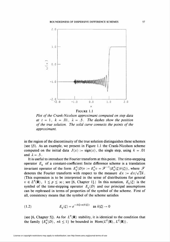
Figure 1.1

Plot of the Crank-Nicolson approximant computed on step data

at t = I, k = .01, X = .5. The dashes show the position

of the true solution. The solid curve connects the points of the

approximant.

in the region of the discontinuity of the true solution distinguishes these schemes

(see §5). As an example, we present in Figure 1.1 the Crank-Nicolson scheme

computed on the initial data J(x) := sign(x), the single step, using k = .01

and X = .5.

It is useful to introduce the Fourier transform at this point. The time-stepping

operator Ek of a constant-coefficient finite difference scheme is a translation

invariant operator of the form Ek(D)v :- Ekv ^r~l(E"k(c;)v(i)), where &

denotes the Fourier transform with respect to the measure dx := dx/v2n.

(This expression is to be interpreted in the sense of distributions for general

v e LP(R), 1 < p < oo ; see [6, Chapter 1].) In this notation, Ek(£) is the

symbol of the time-stepping operator Ek(D) and our principal assumptions

can be rephrased in terms of properties of the symbol of the scheme. First of

all, consistency means that the symbol of the scheme satisfies

(1.2) £*(«-;<ri+o(*|{|)

as k\t\ - 0

(see [6, Chapter 5]). As for LP(R) stability, it is identical to the condition that

the family {Ek(D), nk < 1} be bounded in Hom(Lp(R), Lp(R)).


58 DONALD ESTEP, MICHAEL LOSS, AND JEFFREY RAUCH

It is well known that the set of L (R) stable operators a(D) consists precisely

of those maps whose symbols are in L°°(R) and that

Hfl('D)llz.2(R)-L2(R) = llallL»(R)-

In what follows, we assume that the symbol of a difference scheme is at least

continuous in ¿I. Thus, a necessary and sufficient condition for the stability of a

difference scheme in L (R) is that there exists a C > 0 with \Ek(Ç)\ < I + Ck

for all £ e R, k e (0, 1). For example, the symbol of the Crank-Nicolson

scheme is1 -¿/lsin(«c;)/2

k[Ç) l + //lsin(«0/2'

In this case, ^¿.(¿Ol = 1, so Ek(D) is L (R) stable without condition. If X

is constant, then it is known that Ek(D) is stable in LP(R) only for p — 2.

(Note that the "overshoot" to the left of the step shows that this scheme is not a

contraction on L°°(R), but we show below that the "overshoots" are bounded

as A:-»O.)Since the 1960's, many authors have studied the stability of difference meth-

ods and the conditions which make a scheme dissipative or dispersive, including

Apelkrans, Brenner, Chin, Hedstrom, Peetre, Thomée [1, 4, 5, 6, 8, 9, 12, 13,

18, 22], and Trefethen [23, 24], who presented a nice overview of the subject

and in the case of dispersive schemes made a connection to the classical theory

of dispersion, see Whitham [26].

The analysis of the pointwise behavior of difference approximants becomes

interesting in the case of schemes which are only L (R) stable, and hence

known only to converge in the L (R) norm, because they represent a pointwise

approximation to the true solution. In particular, L°°(R) instability implies,

thanks to the uniform boundedness principle, that there is a v e L°°(R) such

that

sup \\Ek(D)v\\Loo(R] - oo.nk<\

On the other hand, everyday experience does not seem to produce such v.

In particular, if v is piecewise C , but possibly discontinuous, computations

yield families which are uniformly bounded.

The first result we present classifies more precisely the space of initial data

upon which dispersive difference schemes are unbounded. We say that the

difference approximants are uniformly pointwise bounded if

sup \\Ek(D)v\\Loo(R) < Cnk<\

for some constant C.

Our approach is suggested by the observation that an L (R) stable scheme is

also stable in the Sobolev spaces Hs. We ask if taking data in Hs(R)n L°°(R)

suffices to ensure uniform pointwise boundedness of the approximants. The

answer is positive if ^ is large enough since Hs c L°°(R) for s > 1/2. Thus,

it is sufficient to take the data v in some Hs, s > 1 ¡2, to ensure that the

approximants are bounded uniformly in Hs, hence in L°°(R).



However, functions in Hs, for 5 > 1/2, are continuous, and so our motivat-

ing example of a nonsmooth function, J(x), is not locally in Hs for 5 > 1/2 .

It is natural to ask if less regularity will still suffice, i.e., we ask if assuming

that the pointwise bounded data is in Hs locally, for s < 1/2, is a sufficient

condition to ensure that the approximants are uniformly pointwise bounded.

Here, J(x) is locally in HsnL°°(R) for all s< 1/2.

The first result shows that this is not so. The proof demonstrates that condi-2 2

tions made in the L (R) norm and regularity norms based on the L (R) norm

have an inherent weakness in terms of forcing desired pointwise behavior of

the approximants in situations in which dispersion is present.

Theorem 1.1. Let Ek(D) be the operator of a dispersive constant-coefficient dif-

ference scheme which is L (R) stable and satisfies the consistency condition for

ut + cux = 0, c e R, and suppose X = k/h is constant. Then, there exists a

function v e Hs n L°°(R) for all 0 < s < 1/2 such that

sup \\Ek(D)v\\Loc(R) = 00.

Theorem 1.1 is a consequence of a more general theorem that is stated and

proved in §3. In particular, the assumption of a constant mesh ratio is not

needed, and therefore choosing a very small time step size, for example k =

0(« ), does not help to force boundedness. The first part of this proof consists

in showing that the uniform pointwise boundedness of the difference scheme

operator implies that the operator whose symbol is exp(/¿><f ), with p, b e R,

p > 2, p - 1 the accuracy of the scheme and b ^ 0 a fixed constant, is a

bounded operator in Hom(r7inL°°(R), L°°(R)). Then, we produce a function

u e Hs n L°° (R) suchthat

11 lhDß n\\e "11/,°°^) - °°-

Again, thanks to the uniform boundedness principle, this implies that there is

some function in H5 n L°°(R) which causes the difference scheme operator

itself to be unbounded in the same fashion (the function u may not do this).

In §5, we construct a sequence of functions depending on the step size which

does appear to do this in the limit as the step size tends to zero.

Returning to the computations made with the Crank-Nicolson scheme, the

evidence suggests that dispersive schemes are uniformly pointwise bounded on

the step function. Most of the authors mentioned above studied the bound-

edness and convergence of schemes on step data. Such analysis began at least

partly because (1.1) with step data is considered to be a test problem for nu-

merical methods for nonlinear hyperbolic equations. Apelkrans [1], Brenner

and Thomée [5], and Thomée [22], using similar methods, studied difference

approximations to the solution of the equation ut + p(x)ux = 0, and proved

convergence and gave bounds for the approximants everywhere except near the

point of discontinuity, under the assumption that the schemes are LP(R) stable

only for p — 2 and with a constant mesh ratio X = k/h (see [6]). Taking a



different approach for the same kind of schemes, Hedstrom [12, 13] studied

convergence of finite difference approximants of the equation ut + ux — 0 and

gave a precise description of their behavior. In the case of step data, under

the additional assumption, that the scheme have some higher-order dissipative

character (while remaining only L stable), he showed that the approximants

are pointwise bounded.

One conclusion that can be drawn from Hedstrom's result is that for par-

tially dissipative schemes the assumption that the data be piecewise smooth is

sufficient to ensure that the approximants are bounded in L°°(R). We point

out that this result has a wider significance because schemes which yield uni-

formly pointwise bounded approximants on step data, in fact, yield uniformly

pointwise bounded approximants on data chosen in BV. BV is the class of

functions determined by the norm

II/IIbv:=II/IIl-(r) + II^/IItv

that is, BV is the class of L°°(R) functions whose derivatives are bounded

signed Borel measures. More precisely, let Ek(D) be a translation invariant,

L (R) stable operator such that

sup \\E"k(D)J(.)\\L„ < Cnk<\

for some constant C. Then

sup \\Enk(D)v(.)\\La. < C|M|TVnk<\ *

for all u e BV. The proof is easy, but we present it for the reader's convenience

in §4.Hedstrom's proof of the uniform pointwise boundedness of dispersive

schemes with higher-order dissipation makes explicit use of the dissipative term.

This leaves open the question of uniform pointwise boundedness of purely dis-

persive schemes like the Crank-Nicolson scheme. Our next result shows that

these schemes are bounded, as well. We recall that the characteristic function of

a difference scheme is the function e(<j;) := Ek(c¡/h).

Theorem 1.2. Let Ek(D) be the difference operator of a constant-coefficient finite

difference scheme which satisfies the consistency condition for (1.1) and whose

symbol has the property that \Ek(¿¡)\ = 1. Assume further that the characteristic

function of Ek(D) is independent of h and that k/h is constant. Then the

difference scheme is uniformly pointwise bounded on the step function.

There are three points to be made. First, by Theorem 5.2.1 of Brenner et al.

[6], if Ek(D) is not a simple translation operator, then it is unstable in LP(R)

for all p ^ 2. Second, schemes satisfying the conditions of Theorem 1.2 are

therefore uniformly pointwise bounded on data in BV. We do not demonstrate

that dispersive difference schemes are bounded in Hom(BV, BV), and in fact

they are not in general. Last, the method used to prove Theorem 1.2 gives more



information about the difference approximants of a purely dispersive difference

scheme computed on step data. As an example, our analysis indicates at what

speed the oscillations collapse towards the position of the discontinuity and their

limiting height as the step size tends to zero. In §5, we confirm our predictions

with the observed performance of the Crank-Nicolson scheme.

A basic ingredient of the proof is the fact that the behavior of the difference

scheme is determined on two regions. One region is a fixed number of mesh

widths from the discontinuity, and the other range is the complement. We show

that in the limit of the step size tending to zero, the range of lattice points on

the order of « from the discontinuity carries much of the important in-

formation about the difference approximant. For £ in the corresponding range

in Fourier space, we construct a normal form for the symbol of the difference

operator using the Malgrange Division Theorem and ideas from the analysis of

singularities of maps and oscillatory integrals (see Arnol'd [2, 3] as well as [7, 11,

15, 17, 28]). This normal form is readily analyzed by stationary/nonstationary

phase arguments like those of Stein [21] and Wainger [25].

The outline of the paper is as follows. We start in §2 with the proof of

Theorem 1.2. Section 3 contains the proof of Theorem 1.1. The proof of

the claim made about BV above is in §4. In §5 we present the results of

the experiments mentioned above, together with some samples and discussion.

Finally, the appendix contains the technical proof of the construction of the

normal form.

2. Proof of Theorem 1.2

Theorem 1.2 is a consequence of

Theorem 2.1. Let Ek(D) be a translation invariant, L (R) stable finite differ-

ence operator with e(Ç) := Ek(cl/h) satisfying

(2.1) e(£) is independent ofk;

(2.2) e(¿;) is periodic and analytic in a strip around the real axis;

(2.3) |e(i)|sl;

(2.4) lQg(e(í)) = -itf + o(|í|) asÇ^O;

(2.5) ï(i) = e(-i);

where h := Xk, X a fixed real constant. Then,

ixi^rif^di

i

Proof of Theorem 1.2. It is clear that the conclusion of Theorem 1.2 is precisely

(2.6). The properties (2.1), (2.2) and (2.3) follow immediately from the as-

sumption that k/h is constant, the assumptions made on Ek(D) and the fact

that Ek(D) is the operator of a finite difference scheme which implies that e(f)

is a rational trigonometric function. (2.5) is true because e(£) is the ratio of two

(2.6) sup supnk< i x

>.V.jeixiEnk(i)'- < 00.



(2.7) P.V.JeixiEnk(c;)'-

polynomial functions of e' in which the polynomials have real coefficients.

(2.5) implies that loge(¿;) is an odd function. D

Remark. Assumption (2.2) is a natural condition to make on the symbol of a

translation invariant finite difference scheme. In fact, we only need analyticity to

guarantee that log(e(¿;)) has a finite number of zeros in one period. Otherwise,

it would suffice to assume that e(£) is C°° .

The rest of this section is devoted to the proof of Theorem 2.1 and to dis-

cussing some of its consequences. Since the proof is trivial when Ek(D) is a

simple translation operator, we now assume that Ek(D) is truly dispersive, i.e.,

not a simple translation operator. The difference scheme approximant com-

puted from the step data is given by the oscillatory integral

¿xi r« i KSdÇ,

T'We show that this integral is uniformly pointwise bounded and describe its

behavior for x in the vicinity of the discontinuity of the true solution.

Consider first the formula

(2.8) 7(x) = P.V. feixi^-.

The principal value interpretation of this integral is used to make sense of the

integrand for t\ near zero and to yield convergence of the integral over R. A

dispersive difference scheme introduces oscillations whose frequencies increase

with n . The question is: How do the oscillations affect the convergence of the

principal-value integral?

As for (2.8), there are two natural scales (whose precise ranges are determined

by the difference scheme) in (2.7), £ very large and £ close to zero, resp. the

very fine behavior and the coarser behavior of the approximant in x . We use

different techniques to deal with these two contributions. Write (2.7) as

(2.9) P.V. f eix(Enk(^ + P.V. / eixiE"k(tS,J\(\<e/h <* J\i\>e/h C

where e > 0 is small and fixed. We treat each of the integrals in (2.9) separately.

Remark. In x space, the second integral is the major contributor to the am-

plitude of the difference approximant for x within « of the discontinuity and

the first integral is the major contributor for x further away. We show below

that in fact the largest oscillation of the Crank-Nicolson scheme occurs roughly

at a distance of 1.95« away from the discontinuity. This suggests that the

first integral in (2.9) represents the difference scheme in the limit as « —► 0.

Rewrite (2.9) as

P.V. / eixien(hçfê + P.V. / e'x(en(hi)Jh\í\<e £ Jh\(\>e

and change variables, using the fact that j¡ - Xn , to get

(2.10) P.V. / eanxien(çfê + P.V. [ e,nXxien(^.



We treat the second integral first. Start by considering the oscillatory integral

2.11) I(w)(x) := P.V. / eixiw(t;)^-:= lim /J\£\>n £ M^coJn<'\£\>n S. m^°°Jk<\í\<Mk

where w(Ç) is locally integrable and periodic with period 2n

Lemma 2.2. For the integral in (2.11) we have

ÍXÍ ,r,d<2]e w(£,)—,

(2.12) I(w)(x) = h(x) f+n e'xiw(ci)d<l- [^ eixiw(c¡)f(x, Z)di,J— 7i J— n

where h(x) is the periodic function with period 1 whose restriction to the interval

[-1/2, 1/2] is given by

' x+ 1/2, -1/2 <x <0,

«(x)= I 0, x = 0,

x-1/2, 0<x<l/2,

and

f(x,i):= £ e2nimx

(Ç + 2nm)2nm '

where the prime on the summation symbol indicates that the term with index

zero is omitted. Moreover, f(x, <;) is uniformly bounded for -co < x < oo and

{ € [-71,71].

In particular,

supX

P.V.í ix£ r£\d(¡/ e *wß)

J\£\>n<c /4 n

■K

w{i)\dt,'líl>* í

with a constant C which is independent of x and w(Ç).

Proof of Lemma 2.2. For periodic g with period 2n ,

f g(t)dt¡= £' Hg(£ + 27tm)dt\;Jn<\£\<Mn \m\<M J~K

thus the integral on the right in (2.11) is equal to

2nim£ 1

JraKJIi2nm

j^ e'xiw(£) dH - 12 eixiw(Ç)fM(x, Q d£

with

(2.13)

Note that

fM(x,i):= £ e\m\<M

2nimx

\m\<M

2nimx 1

2nm

(£ + 2nm)2nm

h(x) as M -+ oo

pointwise for every x , and the sums are uniformly bounded. Also, fM(x, £)

converges uniformly to the continuous function f(x, ¿f) as M —> oo . D



Now consider the characteristic function e(¿;) of a difference scheme satisfy-

ing the hypotheses of Theorem 1.2. Without loss of generality, we may assume

that e(c¡) is periodic with smallest period equal to 2n . We can arrange this with

a simple change of variables in £, using the unique smallest positive period of

e(¿¡), and since the estimates will be uniform in x , the change to the exponent

of e in the integral in (2.10) can be absorbed into x . Similarly, X also can be

absorbed into x . Hence, we can apply Lemma 2.2 to find that

P.V. / eim\n(Ç)d4-

for all x, X and « . Since for fixed e > 0,

<C

f ei^\\ç&-h<\t\<K £

(2.14) P.V. /

is obviously uniformly bounded by (2.3), it remains to consider

¿n(Xx£+0(£))dC_

'líl<í é

where 6(Ç) denotes the real analytic function which satisfies

e(í) = /e(í)0'(í), 0(0) = 0.

It is easy to see that d(2n) - m2n for some integer m and that e(£) = e' .

Moreover, (2.4) and (2.5) imply that 6 is an odd function and therefore 0(£) =

—A£ + c £,ß -H— , where p is an odd integer greater than one and c / 0. ( p - 1

is the accuracy of the difference scheme, which we have assumed is not a simple

translation operator.)

A is a fixed real number, so replacing « by nX and 6 by 6/X eliminates

X from the integrand in (2.14). Our first aim is to show that this expression is

bounded in magnitude uniformly in « and x . The following lemma is the basic

ingredient for what follows. It applies to a symbol satisfying the hypotheses of

Theorem 2.1 with v :— (p - l)/2.

Lemma 2.3. Let F(£, y) = £y + (0(£) + {), where y := x - I and (0(£) + i) =

0(<^ v+ ) as |i| —> 0, v > 1. There is an open neighborhood O of the origin,

Bj e C°°(0) and e>0 such that P(i,y) := c\2v+x + Yü'l Bj(y)^i+i satisfies

(2.15) supyeo

P.vf ew)K_PmVm[J\£\<e £ J\£\

inP(£,y)d£

J\£\<e' £< c

for some e > 0.

Remark. P(Ç , y) is not uniquely determined.

Proof of Lemma 2.3. By Theorem Al (see the appendix), for £ and y suffi-

ciently small, there exist smooth functions Bj(y), Bj(y) = O(y) as y —* 0,



j = 0, ... , v - 1, and 3(£, y) odd in £ , such that

F(£,y) = E2»+]+Y2Bj(y)Z2j+l=:P(Z,y).

7=0

Hence,

(2.16)

'.V. f iJ\£\<e

JnP(Z(£,y),y)dÇ= P.V. f

J\i\<ß

einPm-yhy)U-%]dÇ

+ P.VJ\£\<\S(e,y)\

mP(£,y)dÇ

£ '

where E = dE/dÇ , and the oddness of E was used. Hence, it suffices to show

that

1 E'(2.17) ---

is bounded uniformly for £, and y sufficiently small. Since E(-¿¡, y) =-S(i,y),

E(i,y)-ÍE'(í,y) = 0(i3)

as <£ —> 0, and by (A-2) in the appendix,

(2.18) = 0(1)

as £ -> 0. Therefore, (2.17) is 0(|£|) as <^ -♦ 0, and (2.15) holds with e' =

Z(e,y). D

Proof of Theorem 2.1. First consider the case when x is taken in a small, fixed

neighborhood around one. By Lemma 2.3 and the estimates made on the second

integral in (2.10), the uniform pointwise boundedness of (2.7) for such x is

reduced to the boundedness of

m(B0£+Bl(3+-+(2,'+l)d^

£

for some /. Since the coefficients B0, ... , Bv x depend on y in an uncon-

trollable fashion, it is crucial to get a bound on (2.19) which depends on v but

not on B0, ... , BvX . Such a result was obtained by Stein and Wainger. The

proof, from [21] and [25], is repeated here for the sake of completeness.

By the definition of P.V., the result follows if the integral

nc0£+cie+-+cX'"tl)dd

(2.19) > V. / e""''

L£<líl</

is shown to be bounded uniformly in c0, ... , cv, I and s. Using the scale

invariance of dl\/t\, we may assume that cv = ±1. By partial integration,

(2.20)f'/S eiicoi+-±(^ 'f = m\

lit

+fl/£ dt


66

where

DONALD ESTEP, MICHAEL LOSS, AND JEFFREY RAUCH

fie ■"e <(c0í+-±í2"+1)

d£.

An application of Van der Corput's lemma (stated below) with j = 2v + 1

shows that /(£) is bounded in magnitude by a constant C(v), and therefore

so is the integral on the left-hand side of (2.20) independently of l/e .

On the other hand,

i

t(c¿+-+c._,e'-l±e»+,)di

e<lil<l /

.'G■¿+-+c,_leb'-l)dt

£<|Í|<1

<-Lt+lf<C(u),'e<\£\<l

independent of £ . Thus, by using induction, the problem is reduced to the case

when 2v + 1 = 1, which is a standard result. D

Van der Corput's Lemma. Let tp e CJ(R[) be real with \y/U)(Ç)\ > ô > 0 on

[a, b]. Then

I■la

e"" dt <C,

with C independent of a and b.

This lemma is proved using the same lemmas of Stein that were used above.

Stein proves the following related proposition in [21].

"Proposition 2". Suppose that </> is real-valued and smooth in [a,b]. If\4> (x)\

> 1, thenrb

jJa

einé(x)dx < c-n 1/7

holds when (i) j > 2 or (ii) j — 1, if in addition it is assumed that 4>'(x) is

monotonie.

"Corollary". Under these assumptions on 4>, we can conclude that

[bein*{x)ip(x)dx

Ja< en

■W\ip(b)\ + j\ip'(x)\dx\,

where y is any smooth complex-valued function.

Remark. That (2.14) is bounded uniformly for x outside of a small neighbor-

hood of one is easier to show. In this case, (Xx£ + &(£,))' = X(x - I) + o(\£\)

is uniformly bounded away from zero for £ in a small neighborhood of zero.

Therefore, one can construct a map E(i£, x - 1 ) with

xXE(¿¡, x - 1) + 0(S(Í, x -l)) = (x- l)X£ + Bcfv+',

for some real constant B, by the implicit function theorem. Then, one proceeds

as above. Of course, it is necessary for |x - 1| to be bounded away from zero,



the boundedness of the integral with the transformed variable will depend on

Ix-ir1Next we prove

Theorem 2.4. For x sufficiently close to 1

limn—>oo

\V. [°° eanixen(çfê-P.V. f einP((-x-J—OO € J—e'

= 0.

In other words, in the vicinity of the discontinuity of the true solution, the

behavior of the difference scheme is determined by the normal form P(<;, x-1 ).

Proof of Theorem 2.4. Thanks to Lemma 2.3, it suffices to show that the second

integral in (2.10) and the first integral on the right of (2.16) tend to zero as

« —> oo, uniformly in Xx . Consider the former integral. Once again, we let x

replace Xx and assume that e(¿;) is periodic with smallest period 2n ; thus we

consider

P.V./ e^\n(Ç)d4-•>iíi>* £

Returning to (2.12), we analyze this expression with w(c\) = e"(¿;), using

stationary and nonstationary phase methods. The stationary phase points of

e e(£) are given by the zeros of the function

ix + ^ = ix + id\i).

It follows from the assumptions made on e(£) that 0"(Ç) is not identically zero

on any subinterval of [-n, n], and because 0 is analytic in a strip around the

real axis, 0"(O has only a finite number of zeros, M, in [-n, n]. Call these

zeros ¿[, ... ,ÇM with multiplicities px - I, ... , pM - I. Choose ó positive

so that 0"(£) has only one zero in each neighborhood A/ = {¿¡\ \Ç - ¿¡.\ < ô}

oî£-,j=l,...,M, and furthermore, so that there exists a constant c = c(S)

such that |0("j)(£)| > c for { e Njt j = 1,... ,M, and |0"(£)| > c for

{ € [-7T, 7t]\[JNj. Since (dJ/d£j)(x£ + 6(£)) = 6U), j>2, these bounds also

hold for x£ + 0(£), independent of x .

In view of (2.12) and (2.13), consider two terms. First,

reitt{xi+m)f(xn,Z)dÇ

(2.21) * +n_ f in{x£+8{£)) yV 27t/mx_£_ ,,

)_n ^ (£, + 2nm)2nm Ç'

Using Fubini's theorem, we can switch the order of summation and integration.

Thus, it suffices to treat

e2mmx r>M+'«» * dt, m¿0,J-n (ç, + 2nm)2nm



separately and then sum the results. We decompose this integral as

M

, J N:

-ö(O) ç

(¿I + 2nm)2nm(2.22) J=x

_,_ f ein(x(+0(())x]\uNj (£- 2nm)2nm

+ [ em(xi+m) ^-^^ dd.J[-n,n]'

Since 0" is of constant sign on each component of [-n, n]\ (j A/ , we can use

the corollary to Proposition 2 of Stein [21] to conclude that the second integral

is bounded in magnitude by

(2.23) Cn~l,2~.

m

By the same corollary, each integral in the sum in (2.22) is bounded in magni-

tude by

(2.24) en ' ' —j.m

Summing (2.23) and (2.24) in m , we see that the integral in (2.21) can be made

as small as we like by choosing « large.

The other term in (2.12) is

ix£n «/c,e e (Z)<-n

h(x) e - e(¿)#.

This can be handled in the same fashion as were the integrals in the sum in

(2.21), now using Proposition 2 of Stein [21] directly, yielding the same asymp-

totic bounds.Using arguments similar to those used to bound the integrals in (2.22), it is

easy to see that the contributions to the second integral in (2.10),

/ iXx£n n , „, dç/ e e (£)-r.

also tend to 0 as « —► oo at the same asymptotic rate uniformly in x and

X for any fixed e > 0. Hence, we conclude that in the limit of the step size

tending to zero, the difference scheme solution is described by the first integral

in (2.10) with an error like 0(«~ ), ß = maxpi.

Now, we look at the first term on the right of (2.16),

f ,mF(S,y)(l Z\ d^

where \/£, - E'/E is a smooth function of ¿¡ and y. Arguments similar to

those above show that this term tends to zero as « —» oo uniformly for x in a

neighborhood of 1 . D

The normal form can be used now to analyze some of the oscillations ap-

pearing in the difference approximant around the discontinuity of the solution.



Since for fixed y ^ 0 the scheme converges to the actual solution, one might

be tempted to ask how quickly the peaks of the oscillations move towards the

discontinuity and how large these peaks can be. In other words, how to choose

x(«), x(«) —► 1 as « —> oo, such that the expression (2.14) deviates substan-

tially from the true solution of the differential equation. The following result

shows that for difference schemes with normal form P the approximate solu-

tion U(l, l+ah v'( l/+ ) is roughly independent of « as « —»0. This suggests

the rate at which peaks collapse towards the discontinuity and gives a formula

which can be used to estimate the heights of the peaks (see §5B).

Theorem 2.5. Let y(n) = an" v'( "+1). Then,

(2.25) lim P.V. f einP^n))d4=P.V. f°° ei{cat+i^,n^°° J-e' £ J-oo £

where

-=t(o)=(f,o'o»r*°-Proof. Since Bj(y) = 0(y), ; = 0, ... , v - 1, changing variables £, —>

n-l/(2,+l)£s

Qn(i,a):=nP(n-l/{2,/+l)c;,y(n))

(2.26) =t+[ +YJB](y(n)W-(2l+{)l(2^X)eHX

7=0

= ç2"+1 + B0(n-2^+i)a)n2^+l)c; + o(l),

which establishes the result provided the interchange of the limit with the prin-

ciple value integral is justified. Obviously, the zeros of (2.26) for a fixed, all

stay bounded inside a circle of radius say R, uniformly in « . Now

lim fp.V. /V»(i'a)$-P.V. /%'■«->«> ̂ J-R £ J-R

(ca(+£2«+,)d£\ =0

by the dominated convergence theorem, observing that Sn(Ç) := e "

ei(ca£+( ) _ q^j uniformly in n and Sn(Ç) -* 0 pointwise as « —► oo.

To treat

P.V./ e'Q^'a)d4,J\£\>R £

rewrite it as

p.v./ ,<Wi * ß^W{121) k\>R \t 2v + \QH(t,a))

+ F.Y.Í ̂ "> * §Í£l£><«,J\i\>* 2v + x QniZ>a)

which is allowed since all of the zeros of Q (Ç, a) lie inside {£\ \£\ < R}.



To interchange limit and integral in (2.27), observe that

Q„{i,a)-zkiQ'„{Z,a)Z

l£|3{(2,«?,«)

for some fixed constant C and that the integrand converges pointwise to

(2.28) ( 1 - -L-V^+'> 2Ja ,y ' \ 2v+\) f^+cat;

and use dominated convergence. The change of variables Ç = Qn(Ç, a) in the

second integral of (2.27) yields

1 „„ f e«dï-P.V. /1 J\£lv+l J\£\>\Q„(R,a)\ £

which converges to

-L-P.V / e**2v + 1 J\i\>\R2"^+caR\ £,

(2-29) 2v

Adding (2.28) and (2.29) yields the result, n

3. Proof of Theorem 1.1

Theorem 1.1 follows once we have proved Theorem 3.1 given below. Thisi>2theorem is stated in terms of the Besov spaces BÍ'9 rather than the Hs spaces

because the Besov spaces are finer.

First, we recall the definition of the Besov spaces.

Definition: Besov spaces B2'q, 1 < <7 < oo, 0 < s. Let {y/ (£), j > 0} be a

set of nonnegative functions with

V0 G C0°°({í: \£\ < 2}), ¥j e C0°°(K: 2J~l < \£\ < 2J+l}),

and J2 Wjit) = 1 • Then, v e L (R) is in Bs2q if and only if

|HBr := \\{2JS\\^ V/)llL3(R)}||MZ+) < oo,

where /?(Z+) is the space of sequences {{c^}, j e Z, j > 0} with the usual

norm.

We note that !?~ (yd) is the "part" of v with frequency close to ±2J,

and that the Besov norm measures the growth of these parts as j; —> oo.

Example 3.1. The integral J(x) in (2.8) is locally in By 'q if and only if

q — oo.

We call these spaces finer because the following inclusions hold:

(J rfcBf cBf-'cB^C f| H*s>\/2 s<\/2



for all q e [1, oo). We note that Hs = B2' .By interpolation, it follows that

L (R) stable difference schemes will be stable in the spaces B2 'q as well. The

sharp Sobolev theorem (see [15]) asserts that functions in B2 ' are continuous

and pointwise bounded. Taking our data in this space suffices to ensure that the

approximants are uniformly bounded in this space, hence in L°°(R), and it is

natural to ask whether taking the data in B2' '°°P\L'X>(R) is sufficient to ensure

uniform pointwise boundedness of the approximants. B2 '°° n L°°(R) is a

small Banach space that allows step discontinuities and is contained in L°°(R).

Recall that along with an assumption of L (R) stability in the difference

schemes, the previous works cited have in common the assumption of a constant

mesh ratio. However, there are schemes for which it is efficient or even necessary

to assume a different relationship between k and « . For example, in the Lax-

Wendroff scheme, we could take k = « , and satisfy the CFL condition. One

might ask if sacrificing efficiency in this way will result in a scheme which is

L°°(R) stable. This is not answered in the existing literature. (See §5 for more

examples.) We state the theorem in a general fashion to widen its applicability

to schemes like these. In particular, we do not assume that there is a constant

mesh ratio. We let <% denote the space B2/2,oc n L°°(R).

Theorem 3.1. Let {Ek(D), 0 < k < 1} be a family of translation invariant,

L (R) stable operators. Assume that the symbols {Ek(¿;)} belong to C°°(R)

and further that there exists a £0 such that

(3.1) \Ek(Zo)\ = U

(3.2) Ek(i0 +Í) = Ek(Z0) exp{ia0kÇ + ib0kUye + kp0(k, £)},

where aQ, bQ, y and p are real, y > 0 and p>2; p0 is a continuous function

with p0(0, Ç) = p0(k, 0) = 0 and

hmp0(k,k-y/fl£) = 0,

uniformly for £ in compact sets.

Then, there exists a ue¿¡8 such that

sup ||££(Z))h||¿00(R) =oo.nk< 1

Remark. Thus, the family of operators {Ek(D), nk < 1} is unbounded in

Hom(^, L°°) and therefore in Hom(Hs n L°° , L°°) for 5 6 [0, 1/2).

Example 3.2. For the Lax-Wendroff scheme with k — h , the expansion at

£ = 0 is

Ek(cl) = exp{-i{* + i*3*2 + kp0(k, £)},

where pQ(k , £) satisfies the hypothesis of the theorem.

The proof of Theorem 3.1 is by contradiction. The following theorem is the

first step.



Theorem 3.2. Let {Ek(D), 0 < k < 1} be the family of operators from the

statement of Theorem 3.1. If there exists a C' > 0 such that

\\Enk(D)\\^^Loo{R)<C' forallnk<l, fee (0,1),

then e\p{ib0nkD"} e Hom(^, L°°) for all nk < 1, k e (0, 1), and further,

there is a C = C(¿¡0) > 0 with

\\exp{ib0nkDfl}\\^^LoO{R)<C for all nk < 1, ke(0,l).

Assuming Theorem 3.2, we conclude that if the family of operators from the

statement of Theorem 3.1 is uniformly bounded in Hom(^, L°°), then the

family of operators {exp{ib0tDp}, t - nk < 1, 0 < k < 1} , where b0 e R\{0}

is constant, is uniformly pointwise bounded on data in S§ . Theorem 3.2 is a

partial analogue of Theorem 5.2.1 of Brenner, Thomée and Wahlbin (see [6,

Chapter 5]). In particular, fix «, t = nk, and set b :- b0t ; then the theorem

implies that the operator exp{ibDß} is in Hom(^ , L°°). After the proof of

Theorem 3.2, we show that the function u,

u(x):=^(e-'bi"^

where k(c¡) e C°° , 0 < k < 1, k = 0 for <J < 1 and k = 1 for f > 2, is in &

and is mapped by exp{/èZ)/'} into 9" («:(£)/£) ^ L°°(R), thereby proving

Theorem 3.1.

Proof of Theorem 3.2. By the assumed expansion of Ek(ü¡,) at £0 , we have

E"k($0 + £) = Enk(£0) exp{iaQt£ + ibQtk7e + tp0(k , £)} ,

where t - nk < 1, 0 < k < 1 . We define

Ëkl(£) := (Enk(Ç0))-1 exp{-iaott}E"k(£0 + Ç).

Using some simple estimates, the boundedness assumption on Ek and the fol-

lowing lemma with l(x, £) = exp(/x<¡;), we conclude that

\\Ëk,,iD)\\^L~m<C

for all k e (0, 1), t = nk < I, where C — C(|¿;0|) is some constant.

Lemma 3.3. Suppose the function /(x,£) has a continuous derivative in x and

is continuous in £, and further, for each ¿I e R, there is a C' - C'(¿¡) such that

max{||/(x, OII,.~(Rt), \\d¿(x, £)||¿~(RJ} < C .

Then, g(x) e ¿% implies l(x, £f)g(x) e & for each £, e R, and further, there

is a C = C(£) such that

\\Hx,Z)g(x)\\a<C\\g(x)\U.



In addition, C may be chosen to be a monotonically increasing function of \£\ ,

so that C is uniformly bounded on bounded subsets of R.

This lemma follows immediately from Theorem 2.1 of Peetre and Thomée

[18]. We now set

%,t(Z)--=Ëk,t(k-y/Mt),

and use

Lemma 3.4. If A(D) e Hom(á? , L°°(R)), then for any constant c > 1,

\\A(cD)\\a_^LcoIK) < \\A(D)\\^^L^(R).

This lemma implies that

(3.3) R,/(ß)llÄ_L«»(R)<C for every/c 6(0, 1), nk = t < 1.

The proof of Lemma 3.4 is postponed for the moment. We need two other

facts, as well. First, note that by the assumed L (R) stability of Ek ,

(3.4) \Ekt(Ç)\<C for every £eR,

for some C. Next,

(3.5) r(/JrC,í) = r(í,0:=exp{íV^}= gmlk>t(í),nk=t

uniformly for x in compact sets. By taking the Fourier transform of both sides

and using (3.2) and (3.3), one can show that

g(t,D)o = S'-limI, ,(D)v ïorveS.n—»oo K-'nk=t

Therefore, for y/ e S, with f\y/\ = 1, using (3.1), we have

\mt,D)o,¥)\<C\\o\\a,

so by the converse to Holder's inequality, <E?(t, D)o e L°°(R) and

(3.6) W(t,D)o\\Lcow<C\\o\\a

for all ue^and t = nk < 1, k e (0, 1).

However, 5 is not dense in S§ (see [6, p. 44]), so the usual completion

argument does not suffice to prove the theorem. Nevertheless, 38 is the dual

of a Banach space, namely,

J = (B2/2JUl'(R))'.

Furthermore, S is weak star dense in 3§ . In fact, it is not hard to show that

if j(x) e C0°°(-l, 1), y(0) = 1, ; > 0, and fjdx = 1, then for u e 33,

un :— (nj(xn)) * (j(x/n)u(x)) converges weak star to u as n —» oo, and

IMU = lim IKII«-



Given «eJ'jWe estimate

W(t,D)u\\Lcow

by choosing un e 3S , as above. Then %(t, D)un -> %(t, D)u in S', so that

\\ÏÏ(t, D)u\\L~m < ïîm||r(i, ß)«„||L-(R) < CÏÎm||MJ|^

using (3.4). Since the right-hand side equals C\\u\\^ , the proof of Theorem 3.2

is complete. D

Proof of Lemma 3.4. We set Ç = c<¡; and compute to find that for ue3$ ,

\\A(cD)u\\L~{R)

^c-'im^ii^^^^ii^'^-'oiIbi/^ + II^'o^'oII^r)) ■

We first evaluate the Besov norm on the right, by using an (equivalent) definition

(see [6]):

ll^",Û(C-1.)||B,/2.oo

(3.7) =||^-'ii(c-1.)||L2(R)

+ supt[/2sup\\3r~iÛ(c~i-)(x + y)-^~lû(c~l-)(x)\\L2(R).í>0 \y\<t y '

To calculate the first term on the right-hand side, use Plancherel's theorem and-i

set n = c i, to obtain

W^ V '•)IIl2(r) = c1/2IIwIIl2(r)-

For the second term, setting Ç = c~ £,, we find that

\\(xy - l)F-lû(c-l.)\\L2(R) = cl,2\\(ei{ycK - 1)0(011^,.

Thus, we get for the supremum in (3.7), using in order the substitutions z = cy

and t = c~]s and also using Plancherel's theorem,

c12 sup?1/2 sup \\(el{yc)i - l)û(C)||,2(R , = sups1/2 sup \\u(x + y) - w(x)||L2(R).t>0 \y\<t K c' i>0 \y\<s K

Since c > 1 , we conclude that

||^'~1m(c~'-)||bi/2.«' < c1/2||m||bi/2.oc .

To complete the estimate for \¡F~ û(c~ -)ll,#>weset Ç = c~ Ç and estimate

11'^" UiC *) liz.°°(R) = CIIMII/_°°(R) •

Finally,

||^(cZ))M||L«,(R)<c_1p(Z))||^_^(R){c1/2||w||B,,2.TO + c||k||lco(H)}

<M(D)||^t-m||«IU.This is the desired inequality, n



Proof of Theorem 3.1. As remarked after the statement of Theorem 3.2, it

suffices to show that the distribution u e S'(R) whose Fourier transform is

e k(<£)/<£, p > 2, satisfies u e 33. That u e B2 3 is immediate. It re-

mains to show that u e L°°(R).

We interpret this distribution as a principal-value integral, finding that

u(x) = P.V.[eixieii"^dí= lim /Ví+°^.J £ R^ooJo f

We analyze the last integral by the same methods used in the previous section.

Since k(£,)/£, is a smooth function, we can apply the corollary to Proposition 2

of Stein [21] with j - p to find that

|/0>^iH-(w"?4where C is independent of R . Taking the limit as R —► oo shows the result. G

4. BOUNDEDNESS OF FUNCTIONS IN BV

This section contains the proof of the claim concerning the step function and

BV made in the introduction. Our assumptions imply, first, that Ek is uni-

formly pointwise bounded on the characteristic function #(x) := ^((-oo, x])

and, second, that it suffices to show that the claim holds for all functions

v e NBV (the class of functions which are of bounded variation and nor-

malized in the sense that they are left continuous at every point of R and have

a limit of zero at -oo ). In this case, v e NBV can be written

v(x)= Xxdpv,Jr

where pv is a signed Borel measure with / \dpv\ = ||w||TV < oo .

Choose \p e S with / |^| = 1 and consider the definition of Ek(D)v as an

element in S' :

[E"k(D)v, y,) = (v,E"k(-D)w) = (J Xx dp,,, E¡(-D)¥(x\'k

Using Fubini's theorem to switch the order of integration,

,«\(E'k(D)v,tp)\ j dpv(Xx,Enk(-D)tp) < cIMItv

which proves the result by the converse to Holder's inequality. D

5. Experiments, examples and discussion

In this section, we present the results of some numerical experiments and

examples which illustrate some of our results.



A. A computation suggested by Theorem 1.1. The following experiment shows

initial data bounded in 3§ for which the Crank-Nicolson scheme for ut+ux = 0

yields unbounded approximants as h —► 0 while / and X remain fixed. For k

and « fixed, Ek(D), being smooth and having a periodic symbol, is a bounded

operator from L°°(R) into itself. In particular, Theorem 5.3.1 of Brenner et

al. [6] shows that

II£>)IIl~(r)^l~(R) = o("1/2)-

On the other hand, the dispersive character of the Crank-Nicolson scheme

yields the inequality

(5.1) II£*v0)Hz.~(rh¿~(R) >cn12.

Trefethen presents a nice explanation of this in [23, 24]. He argues that a

carefully constructed spike function vh(x) with height 1 and width 0(1/«) is

sent by the backward Crank-Nicolson scheme with symbol

E"k(-D) = E"k(D)* =E"k(D)~l

(note that Ek(D) is L (R) unitary) to a wave packet that is uniformly dis-

tributed over an interval of width O(t). Thus, there is an increase in width of

O(n), and since the L (R) norm is preserved, the height suffers a decrease of_i i-y

0(n ' ). Taking the resulting functions as initial data for the forward scheme

yields (5.1).

We have to be a little more careful in order to show that

ii^r^ib^L-tR)-*00-

Start with the simple spike function

( x/h + l, -h <x < 0,

vh(x) := I -x/h +1, 0 < x < h,

0, \x\>h,

with (ignoring multiplicative constants)

_ 1 - cos(«£)

*(í) ~ he •It is easy to verify that vh and Ek(-D)vh are bounded below in the B2 '°°

norm, and so in the 3§ norm, independently of h . Thus, taking the functions

Ek(-D)vh as initial data does not suffice to show that

ll£'*:(ö)II.^^Z.00(R)

is unbounded as k —> 0.

To get around this, truncate the Fourier transform of vh by setting wh(x) :=

■^-\vh(í)x(£)), X(£) = X(£,h), XeC°°(R)xC°°(R), X(t)= 1 for |£| <

1/« 5 and xi£) — 0 f°r l£l > l/w'5 + e, for some e > 0. It is easy to see that

\\Eli-D)whh^-°° = IKIIBj/2-~ =°("1/2)



3.0

2.0

1.0

¿ 0.0J

-1.0

-2.0

-3.0-3.0 -1.5 0.0 1.5 3.0

x

Figure 5.1

Plot of the initial data uh .

h = 2'7, X = .5, t = 0.

as « —► 0. Next, set

s Enk(-D)wh(x)

U»(X) ■ \\E"k(-D)wh(x)\\^{R) •

uh is bounded in 33 independently of «, and since \\Ek(-D)wh\\Lao{R) =

0(«1/2), it follows that

\\uh(x)\\^ = l+0(hU2).

Therefore, uh will produce the desired behavior in the approximants.

Unfortunately, uh{x) is not the regularly shaped wave packet (see Figure

5.1) that Trefethen's argument requires. Thus, we might expect that the forward

Crank-Nicolson scheme used on the data uh produces a height increase of only

0(«r>) for some a < 1/2. This appears to be the case. For the numerical

experiments, we approximate the integrals defining wh(x) for h = 2" '', i =

1, 2, ... , 6, by the fast Fourier transform, and use the result to compute uh by

the formula above. We use the Crank-Nicolson scheme with periodic boundary

conditions at x = ±2 .

Figures 5.1 and 5.2 contain plots of the functions uh and Ek (D)uh versus

x computed at time t = nk. The focussing of the wave train into a spike is

clear.


78 DONALD ESTEP. MICHAEL LOSS, AND JEFFREY RAUCH

3.0 i—

2.0 —

1.0 —

* 0.0 —

J

-1.0 —

-2.0 —

-3.0 -1.5 0.0 1.5 3.0

x

Figure 5.2

Plot of the Crank-Nicolson approximant computed on the initial

data u, .hi

« = 2~\ X = ,5, t=\.

Since we expect that

\\Enk(D)uh\\^=0(h7a),

we have computed a least squares line fit using as data the log of the ratio of the

maximum heights of the functions to the height of the function with the largest

step size 2" versus the log of the ratio of the corresponding steps. The result

suggests that a ~ .331 with a correlation factor of .994. See Figure 5.3.

It is clear how to construct such a set of functions for some other purely

dispersive scheme. Partially dissipative schemes like the Lax-Wendroff schemes

are another matter, however. The higher-order dissipative effect limits the range

of x over which dispersion is dominant. However, it can be shown that this

range increases in size as h tends to zero, and this fact can be used to construct

examples which show unbounded behavior as for the Crank-Nicolson scheme.

B. Experiments suggested by Theorem 1.2 and the material in §2. Next, we

present three experiments which suggest the usefulness of the normal form for

predicting the behavior of the difference scheme. In particular, for the Crank-

Nicolson scheme discussed above, we use the normal form to give estimates

of: ( 1 ) the speed at which the largest peak moves toward the position of the

discontinuity as h —> 0; (2) the limiting height of the approximants; and (3)

the height of the approximate solution at the point of discontinuity.



2.0

2.0

(È)-log| ^

Figure 5.3

Plot relating the logarithm of the increase in height of the ap-

proximant from t = 0 to t — 1 to the logarithm of the step

size. The diamonds represent the measured points. The dashes

represent the least squares fitted line.

We use Theorem 2.5 as the basis for our predictions. By that theorem, if

x - 1 = 0(«2/3), then in the limit as h —> 0 the difference scheme approximant

will differ significantly from the true solution. The first result we present in

Figure 5.4 compares the distance of the largest peak to the position of the

discontinuity of the true solution to the step size. Since we expect that the

distance goes like ah , we plot the log of the distance versus the log of the step

size for « = .2, .1, .08, ... , .02, .01, .008, ... , .002. We have computed a

least squares line fit for this data and found that |a| « 1.95 and ß ss .67 with a

correlation of .998 . Note that the true peak can be located only to an accuracy

of ±« for a given step size.

From Theorem 2.5, the limiting height of points which satisfy (x-1) = ah

will be given by the integral

(5.2) s/(cTt JO

sin(ca<¡; + £dH,

where c is a constant generated in the construction of the normal form. If we

consider sf as a function of ac, then it is equal to a primitive of the Airy

function Ai(x) := £F~ (e ) evaluated at ac, and therefore the maxima and

minima of sf occur at the values of ac which are zeros of the Airy function.



O

O'

O''

o-'o. o'

.o'

"'S.0 1.5 3.0

-log(h)

Figure 5.4

Plot relating the logarithm of the distance of the largest peak of

the approximant to the position x = 1 to the logarithm of the

step size. The diamonds represent the measured values. The

dashes represent the least squares fitted line.

These zeros are located along the negative part of the axis at well-spaced inter-

vals (see [15]), and therefore the oscillations in the approximant located on a

scale of « will be more or less regularly spaced and their limiting height can

be obtained from stf .

When the symbol is analytic (which is true of the difference schemes con-

sidered), one can construct a normal form which is obtained by an analytic

map and which is unique. In the C°° category, though the normal form is

not unique, the coefficients Bj(y) do have unique Taylor series and thus the

constant c above is uniquely determined. In the analytic case, the normal form

can be constructed by different means (see Arnol'd [3]); the alternative method

yields precise information about the final normal form immediately. For exam-

ple, the symbol of the Crank-Nicolson operator has the Taylor expansion

(5.3) Ek(i) = ei{-V*+*hi*>+-) for X = \,

and the relevant part of the analytic normal form on the scale of h2/3 is given

by e-'at+'*e . This gives c = -(f )1/3.

We substituted the values a = -1.95 measured directly from the approxi-

mants computed above and this c into (5.2) and then approximated the integral

using Romberg integration over a range of [0, 10] and obtained the number

-1.54. (We checked that the truncated range was sufficiently large by comput-

J . u



ing over intervals with right-hand points ranging from 5 to 10 and obtained

the same result to three places each time.) Below, we list the heights at the

peaks for the values of « used to determine the speed of the peaks:

step size «

.2

.1

.08

.06

.04

.02

.01

.008

.006

.004

.002

height of the largest

peak-1.64-1.60

-1.56-1.58-1.58

-1.55

-1.55-1.55

-1.55

-1.55

-1.55

The data support the conjecture that if xn is the measured value of the

location of the largest peak of the approximant and a comes from the analytic

normal form then1

ah2/31 OO.

Another prediction that is easy to make is the height at which the approximant

crosses the point of discontinuity. We take the limit as a —► 0 from above in

Theorem 2.5 and are left with computing the oscillatory integral

ipv f/^.lfÉÊ^.nr sinW 1n 3

The last equality is true because the integral on the right is just the value of the

limit of the translated step function as x 1 1 . For comparison, we present a

chart of the crossing points for the approximants computed above.

step size h

2.1

.08

.06

.04

.02

.01

.008

.006

.004

.002

height at x = 1

36.35.35

.35

.18

.22

.24

.34

.34

.34

.33


82 DONALD ESTEP, MICHAEL LOSS. AND JEFFREY RAUCH

2.0

2.0

Figure 5.5

Plot of the Lax-Friedrichs approximant computed on step data at

t = 1. k = .01, X = .5. The dashes show the position of the true

solution. The solid curve connects the points of the approximant.

Again, there seems to be good agreement between these data and the predicted

height. (As for all of the results, the actual location of the crossing point is

determined only to within ±«, and all of the values above fall well into the

range of heights associated with this error.)

C. Some examples of difference schemes. Finally, we present some examples of

difference schemes.

Example 5.1. The Lax-Friedrichs scheme for ut + ux — 0 is given by

U((n + l)k, jh) - (U(nk, (j +l)h) + U(nk, (; - l)h))/2

kU(nk,(j+l)h)-U(nk,(j-l)h)

+ 2« ~U-

The corresponding time stepping operator is

_ (l-X) , (l+X) ... kEk = ^—x_h + ^—xh, with¿:=p

The operator Ek of the Lax-Friedrichs scheme is a contraction in LP(R), for

1 < p < oo, provided the Courant-Friedrichs-Lewy (CFL) condition k/h < 1

is satisfied. The associated maximum principle is visible in the results of a

computation presented in Figure 5.5 with k = .01 and X = .5 .



2.0

1.0

* 0.0

3

-1.0

-2.0-2.0 -1.0 0.0 1.0 2.0

x

Figure 5.6

Plot of the Lax- Wendroffapproximant computed on step data at

i=l. k = .01, X = .5 . The dashes show the position of the true

solution. The solid curve connects the points of the approximant.

Example 5.2. The Lax-Wendroff scheme for ut + ux = 0 is given by

U((n+l)k,jh)-U(nk,jh) U(nk,(j + l)h)-U(nk,(j-l)h)

k 2«_ k U(nk, (j+l)h)-2U(nk,jh) + U(nk, (j - l)h)

~ 2 h2

and its operator is

£lMi-AV + ̂ _, + ̂ .

The symbol of the Lax-Wendroff scheme is

Ek(Z)= 1 — A2(l - cos(c¡h)) - iXsin(£h).

The Lax-Wendroff scheme is stable in L (R) provided X < 1. If X is assumed

constant, then it can be shown that Ek(D) is stable in LP(R) only for p = 2.

In Figure 5.6, we use the Lax-Wendroff scheme on a single step with k = .01

and X = .5 .

Example 5.3. The following schemes are examples of methods which have a

nonlinear relationship between h and k . First, if we take the equation ut +

ux = 0, and apply the difference scheme which uses a forward time difference



and a centered x difference:

U((n + l)k,jh)-U(nk,jh) U(nk,(j+l)h)-U(nk,(j-l)h)

k 2«

then its symbol is Ek(£) = 1 - /f sin(c¡«). A simple computation shows that we

need to assume that k < ch2 to have L (R) stability. For this scheme, with

k = « , the expansion at £,0 = 0 is

Ek(t) = expi-iÇk + tf3k2 + kp0(k, £)},

where p0{k , x) satisfies the hypotheses of Theorem 3.1. Another example: in1 I")

the Crank-Nicolson scheme, we can take k » h, say k = « , and still have

L (R) stability. The expansion at £0 = 0 for this method is

Ek{H) = exp{-/a + ¿{V + kp0(k, Í)},

where p0(k, £) satisfies the hypotheses of Theorem 3.1.

All computations were performed on an IBM PS/2 50 with a math coproces-

sor using Microsoft FORTRAN 4.0, HGRAPH graphics library and MATHCAD

2.0.

Appendix A. Reduction to normal form

In this section, we prove the main technical result which is used to bring the

phase function into a simple form called the normal form. We follow the proof

given in Hörmander [15].

Theorem Al. Let F(£, y) = £f(£ , y), where f(n, y) is C°° in a neighbor-

hood of the origin in R x R. Assume that

f(n^) = nfin),

where f(0) > 0. Then there exist functions E(n,y) and BAy), j = 0, ... ,

v - 1, C°° in a neighborhood of the origin, such that

F(i,y) = E2v+i+Y(Bj(y)E2j+l,

7=0

with the properties that BAy) = 0(y) as y -> 0, E(Ç,y) is odd in Ç, i.e.,

E(-¿¡, y) = -E(£, y), and furthermore

i-i ™E(0,0) = 0 and |=(0,0)>0.

Remark. This theorem was proved for the analytic case by Levinson [17],

Chester et al. [7] and Arnol'd [2, 3]. The above result is a consequence of the

Malgrange Division Theorem and is due essentially to Mather (see [15, 28]).

We state the Malgrange Division Theorem without proof.



Theorem A2 (Malgrange Division Theorem). Let h(n, y) be a real-valued C°°

function in a neighborhood of zero in RxR". Assume that

h(0,0) = ^-(0,0)=-- = ^—^(0,0) = 0 and ÇlïO.dt] Qrf » dn

Let g(n, y) be any real C function. Then there exist functions q(n,y),

Pj(y)> j = l, ... ,v - l, all C°° in a neighborhood of zero, such that

!/-i

sin, y) = Qin, y)h(n, y) + ̂ pfiyW ■7=0

Corollary A3. Let H(£, y) - h(£ , y), where h satisfies the assumptions of the

theorem above. Let G(Ç, y) = Çg(Ç , y), where g can be any C°° function.

Then there are functions Q(¿;, y) = £,q(£, , y) and pAy), j = 0, ... ,v -I, all

C°°, such that

v-\

G(Z,y) = Q(t,y)H(i,y) + X>70^+1 •7=0

Remark. The main interest of this corollary is that Q(Ç, y) is odd in £.

Proof of Corollary A3. An application of Theorem A2 to the pair of functions

g(n,y) and h(n, y) yields

gin » y) = Qin, y)h(n, y) + ^Pjiy)nJ,7=0

for C°° functions q and p¡, j = 0, ... , v — 1. Replacing « by £, and

multiplying by £, yields the result. D

Proof of Theorem Al. Assume that f(n,0) = rf, i.e., F(¿., 0) = £2v+x ; this

can be arranged by a smooth change of variables. The aim is to find functions

Ç(y) and b(y) (b := (b0,... , &„_,)) of y in a neighborhood of zero, such

that

(A-l) F(£,y) + Y,bJ£2j+X

7=0

is constant. To construct them, differentiate (A-1 ) with respect to y to get

(A-2) \Fi + J2(2j + l)b/J) H' + Fv + £ b'/J+iV '=0 / '=0

(the prime denotes differentiation with respect to y ). By assumption, the first

bracket is an even function of t\, i.e., of the form «(£ , y, b), for some smooth

« . Likewise, F = £g(£, , y, b) for some smooth g. Applying Corollary



A3 to this pair of functions, we find Q(t¡, y, b) smooth and pAy, b), j =

0, ... , v - 1, smooth such that

Fy = Q- U + D2> + 1)¥2J I +/Zpjiy^)£2j+X,V ;'=o J 7=o

where Q is odd in t¡: Q(-¿¡, y, b) = -Q(Ç, y, b). Inserting this formula into

(A-2), the desideratum is achieved, provided that £, and b are chosen to be

solutions of the differential equation

t' = -Q(Ç,y,b), b' = -p(y,h).

Since Q and p are smooth in a neighborhood of the origin, there exist smooth

solutions £,(E, y, B) and b(B, y) having E resp. B as initial data, i.e.,

(A-3) £(E,0,B) = E and b(B,0) = B.

By (A-3), fg(B, 0) = 1. Therefore, by the implicit function theorem, there

exists a smooth function B(y) such that

(A-4) b(B(y),y) = 0

for y in a neighborhood of zero. Obviously, B(0) = 0. This, together with

(A-l), yields

u+\

(A-5) F(Ç(E,y,B(y)),y) = E2"+l + £b.(j;)E27+1 .

7=0

We also used that F(E,0) = E2l/+l .

Finally observe that by (A-3), again using the implicit function theorem,

£(E, y, B(y)) can be inverted to yield E(£, y, B(y)), depending smoothly on

y in a neighborhood of zero. Since Q is odd in £, -£(-E, y, B) is also a

solution with the same initial data and hence £(-E, y, B) = -£(E, y, B) in

the whole neighborhood of existence. Therefore,

E(-Z,y,B(y)) = -Z(Ç,y,B(y)).

Since §§(E, 0,0) = 1, ||(0, 0,0)= 1 as well; this, together with (A-5),

yields the desired result. D

Acknowledgment

We thank Stig Larsson, John Mather and David Stewart for helpful discus-

sions.

Bibliography

1 M. Y. T. Apelkrans, On difference schemes for hyperbolic equations with discontinuous initial

values, Math. Comp. 22 (1968), 525-539.

2. V. I. Arnol d, Singularities of smooth mappings, Russian Math. Surveys 23 (1968), 1-43.

3. _, Singularity theory. Cambridge Univ. Press, New York, 1981.



4. P. Brenner and V. Thomée, Stability and convergence rates in if for certain difference

schemes, Math. Scand. 27 (1970), 5-23.

5. _, Estimates near discontinuities for some difference schemes, Math. Scand. 28 (1971),

329-340.

6. P. Brenner, V. Thomée, and L. Wahlbin, Besov spaces and applications to difference methods

for initial value problems, Springer-Verlag, New York, 1975.

7. C. Chester, B. Friedman, and F. Ursell, An extension of the method of steepest descents,

Proc. Cambridge Philos. Soc. 53 (1957), 599-611.

8. R. C. Y. Chin, Dispersion and Gibbs phenomenon associated with difference approximations

to initial boundary-value problems for hyperbolic equations, J. Comput. Phys. 18 (1975),

233-247.

9. R. C. Y. Chin and G. W. Hedstrom, A dispersion analysis for difference schemes: Tables of

generalized Airy functions. Math. Comp. 32 (1978), 1163-1170.

10. D. J. Estep, L°° bounds for families of translation invariant, L stable operators in one

dimension, Ph.D. thesis, The University of Michigan, 1987.

U.M. Gollubitsky and V. Guillemin, Stable mappings and their singularities, Springer, New

York, 1973.

12. G. W. Hedstrom, The near-stability of the Lax-Wendroff method, Numer. Math. 7 (1965),73-77.

13. _, The rate of convergence of some difference schemes, SIAM J. Numer. Anal. 5 (1968),

363-406.

14. L. Hörmander, Estimates for translation invariant operators in Lp spaces, Acta. Math. 104

(1960), 93-140.

15. _, Linear partial differential equations, vol. 1, Springer-Verlag, New York, 1983.

16. F. John, Partial differential equations, 4th ed.. Springer-Verlag, New York, 1982.

17. N. Levinson, Transformation of an analytic function of several variables to a canonical form,

Duke Math. J. 28 (1961), 345-353.

18. J. Peetre and V. Thomée, On the rate of convergence for discrete initial value problems,

Math. Scand. 21 (1967), 158-176.

19. R. D. Richtmyer and K.. W. Morton, Difference methods for initial-value problems, 2nd ed.,

Interscience, New York, 1967.

20. W. Rudin, Real and complex analysis, McGraw-Hill, 1974.

21. E. M. Stein, Oscillatory integrals in Fourier analysis, in Beijing Lectures in Harmonic Anal-

ysis (E. M. Stein, ed.), Princeton Univ. Press, Princeton, N.J., 1986, pp. 307-355.

22. V. Thomée, On the rate of convergence of difference schemes for hyperbolic equations, Nu-

merical Solution of Partial Differential Equations. II (B. Hubbard, ed.). Academic Press,

New York, 1971, pp. 585-622.

23. L. N. Trefethen, Group velocity in finite difference schemes, SIAM Rev. 24 (1982), pp.113-136.

24. _, Dispersion, dissipation and stability, Numerical Analysis (D. F. Griffiths and G. A.

Watson, eds.), Longman, 1986.

25. S. Wainger, Averages and singular integrals over lower dimensional sets, Beijing Lectures

in Fourier Analysis (E. M. Stein, ed.), Princeton Univ. Press, Princeton, N.J., 1986, pp.

357-421.

26. G. B. Whitham, Linear and nonlinear waves, Wiley, New York, 1974.

27. K. Yosida, Functional analysis, 6th ed., Springer-Verlag, New York, 1982.

28. E. C. Zeeman, Catastrophe theory: Selected papers, Addison-Wesley, Reading, Mass., 1977.

School of Mathematics, Georgia Institute of Technology, Atlanta, Georgia 30332

(Estep and Loss). E-mail: [email protected]; loss @math.gatech.edu

Department of Mathematics, University of Michigan, Ann Arbor, Michigan 48109

(Rauch). E-mail: [email protected]


boundedness of dispersive difference schemes · boundedness of dispersive difference schemes 59...

Documents