Breakdowns Happen: How to Factor Downtime into your Simulation

“One of the most debatable pieces of data that goes into a simulation is the stochastic behavior of machine downtime”. Simulation expert Brian Harrington explains the key learning points simulation modelers should consider when working with downtime.

Early in my career at Ford Motor Company as a simulation engineer I remember building

simulations of our plants and wondering what values to put in for the downtime. In addition, I was

also unsure of what distributions to use or why there were default distributions within the software.

What was the impact of populating the simulation with breakdown behavior? It didn't take long to

realize that downtime had significant effects upon the overall throughput. This article explains the

key factors that should be considered when working with breakdowns within your simulation.

When considering downtime, the starting point should be to consider the following questions (see

Appendix A for definitions):

1. How often does a machine fail (MTBF)?

2. How long does it take to repair it (MTTR)?

These two questions may seem simple, however are often abstracted within the forest of

machinery and clouded by human behaviour. When a breakdown occurs on a machine, it‟s likely

there is time associated with certain phases of a typical repair such as; reaction time, lockout

procedure, actual repair and the start-up.

These repair phases are sources of large variation that can make the determination of a realistic

MTBF & MTTR difficult. Why is “Availability” such an important piece of data? Because it causes

random loses of potential „working time‟; which in turn can cause losses of overall system

throughput. These breakdowns cause “Performance” issues within the system; often captured

within the following two states: “Wait” and “Block”.

Once a team enters downtime figures into their simulation they become concrete (at least for the

particular scenario). Downtime figures will always reduce the respective machines capability and

cause potential performance issues with adjacent machinery, or worse yet a bottleneck. Hence,

companies might have to work additional overtime hours to make up for the lost capacity. In this

paper we will explore some of the most useful considerations when deciding on realistic downtime

data for a typical manufacturing simulation.

2

Capture downtime at station or line level?

A key consideration when building a simulation is whether to record downtime at the station or line

level. The recommendation is to align it with safety lockout zones. A facility might have a lockout

procedure that shuts down a line, or zone within a line, when a repairman enters the zone. Often

lockout zones are based on the electrical drops that are powering the lines. For example, an

automotive line might have 8-stations with 2-lockout zones (see Figure 1). Therefore, when a fault

occurs within a particular station the entire lockout zone will go down. This is easily captured within

SIMUL8 using “Groups” and “Multiple Breakdowns”.

Figure 1: Using Groups and Multiple Breakdowns.

The above example uses downtime data at the station level, but it is captured within the Group

which represents the Lockout zone. The same effect could also be accomplished without using

“multiple breakdowns” by rolling up all the respective downtimes into one aggregate value. This

technique would assume that you have access to the station level data and would simply use the

mathematical calculations in the box below (see also Appendix A). Industrial engineers often use

these equations at the component level to calculate MTBF and MTTR values for stations based on

the stations content such as; number of robots, number of end-effectors and number of clamps that

have been designed into the station.

The above calculations can be accomplished using Microsoft Excel.

3

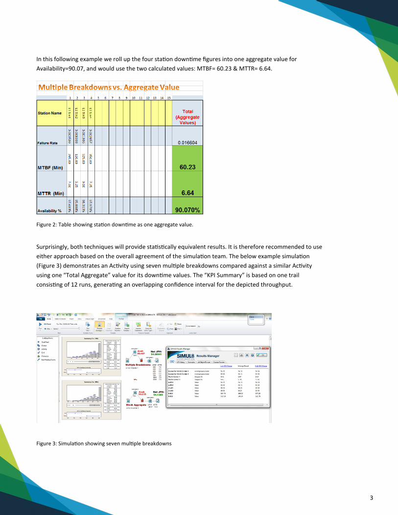
In this following example we roll up the four station downtime figures into one aggregate value for

Availability=90.07, and would use the two calculated values: MTBF= 60.23 & MTTR= 6.64.

Figure 2: Table showing station downtime as one aggregate value.

Surprisingly, both techniques will provide statistically equivalent results. It is therefore recommended to use

either approach based on the overall agreement of the simulation team. The below example simulation

(Figure 3) demonstrates an Activity using seven multiple breakdowns compared against a similar Activity

using one “Total Aggregate” value for its downtime values. The “KPI Summary” is based on one trail

consisting of 12 runs, generating an overlapping confidence interval for the depicted throughput.

Figure 3: Simulation showing seven multiple breakdowns

4

What distributions are associated with MTBF & MTTR?

It is recommended to use the widely recognized Exponential and Erlang distributions. These are proven

shapes that capture the randomness, range and provide realistic samples around the mean. If we examine

an Exponential Distribution using SIMUL8’s “Stat::Fit” we can see what a typical curve might resemble for a

MTBF. Notice when the standard deviation and mean are statistically equivalent we have an Exponential

distribution (Figure 4).

Figure 4: Exponential distribution.

Now that we have a curve that represents how often a failure occurs. Let’s look at what shape would be

appropriate to capture: “How long does it take to repair?” This is where the Erlang distribution fits; it has a

shape parameter that creates a nicely skewed distribution which again captures a wide range of typical

repair times. The below example uses “Stat::Fit” to examine a typical repair time of 7 minutes. Notice that

the Erlang can provide samples that reach out towards possible catastrophic samples such as 40 minutes

(see Figure 5). This type of curve provides the shape that mirrors many realistic repair times. There are many

values that fall below the mean which capture the minor occurrences, i.e. setting a reset button. The skewed

tail provide samples which require more sophisticated repair actions such as; possible electricians,

millwrights, etc. When using the Erlang distribution for repair times the shape parameter “k” is often set to 2

or 3.

Figure 5: Erlang distribution.

5

What about the time to react & travel?

We had mentioned that some simulation teams might want to include the time to react and travel to the

faulted line. This can be accomplished with SIMUL8’s “Combination” Distribution, which in this case would

use two named distributions. The first distribution represents the repair time; and the second distribution

captures the time to react & travel. The time to react & travel might be captured using a normal distribution

with an average of 3 minutes. The “Combination” Distribution simply adds the two respective sample values

together for a total value (Figure 6). The combination distribution allows the user to add as many “Named”

distribution as desired. Therefore, you could even use an additional distribution splitting up the reaction

and travel time.

Figure 6: Combination distribution.

How do we account for the Lockout Procedure?

A lockout procedure might be assumed to be followed on the lengthier repairs such as repair times that take

10 minutes or more. For example the lockout procedure time could be represented as a Normal Distribution

using an average of 3 minutes and a standard deviation of 2.5. Hence, the average of 3 minutes would be

added to all repair times that are greater or equal to 10. This will capture the time to lockout the equipment

according to the companies safety protocol. The resulting distribution will be in the form of a bimodal

distribution, where you will distinctly see the Erlangs’ tail values pick up the additional lockout time (Figure

7). This type of bi-modal distribution can be created in a separate simulation model; which uses the

referenced Visual Logic on Time Check. The Time Check is invoked every minute, and the simulation runs for

2000 minutes; thereby producing 2000 samples within a spreadsheet. The spreadsheet can then be copied

into a Probability Profile distribution within the overall simulation; capturing a particular lockout procedure.

Figure 7: Bimodal distribution.

6

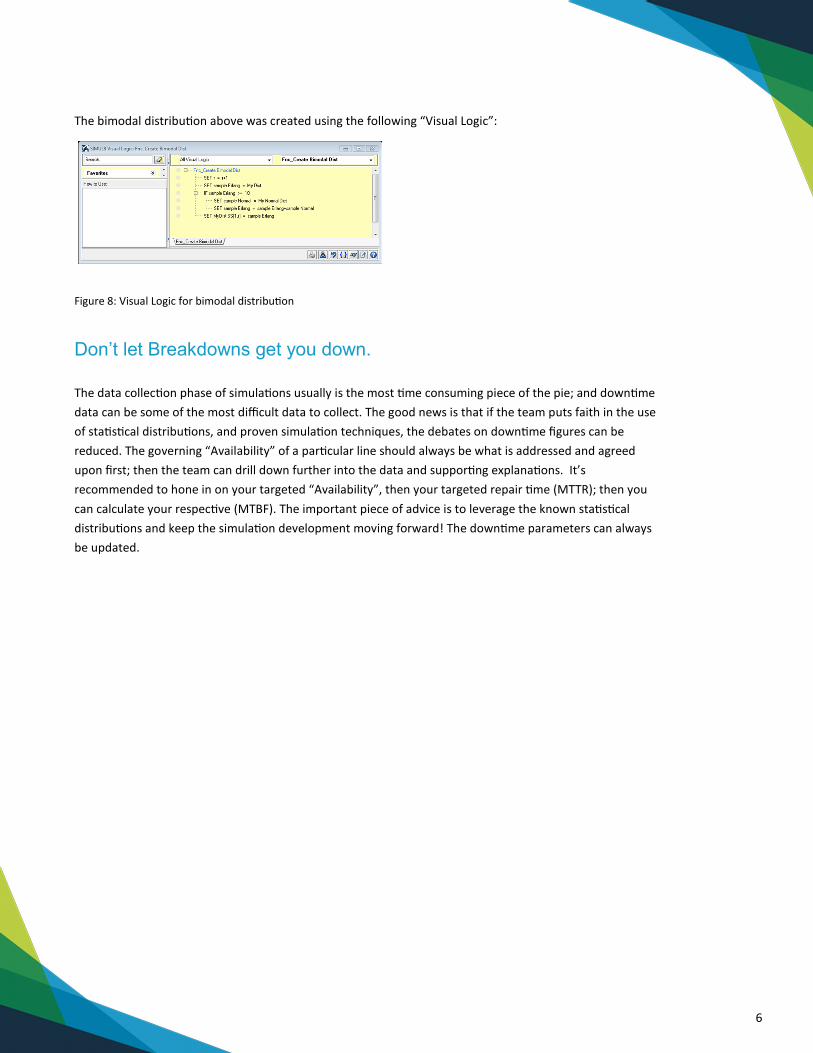
The bimodal distribution above was created using the following “Visual Logic”:

Figure 8: Visual Logic for bimodal distribution

Don‟t let Breakdowns get you down.

The data collection phase of simulations usually is the most time consuming piece of the pie; and downtime

data can be some of the most difficult data to collect. The good news is that if the team puts faith in the use

of statistical distributions, and proven simulation techniques, the debates on downtime figures can be

reduced. The governing “Availability” of a particular line should always be what is addressed and agreed

upon first; then the team can drill down further into the data and supporting explanations. It’s

recommended to hone in on your targeted “Availability”, then your targeted repair time (MTTR); then you

can calculate your respective (MTBF). The important piece of advice is to leverage the known statistical

distributions and keep the simulation development moving forward! The downtime parameters can always

be updated.

7

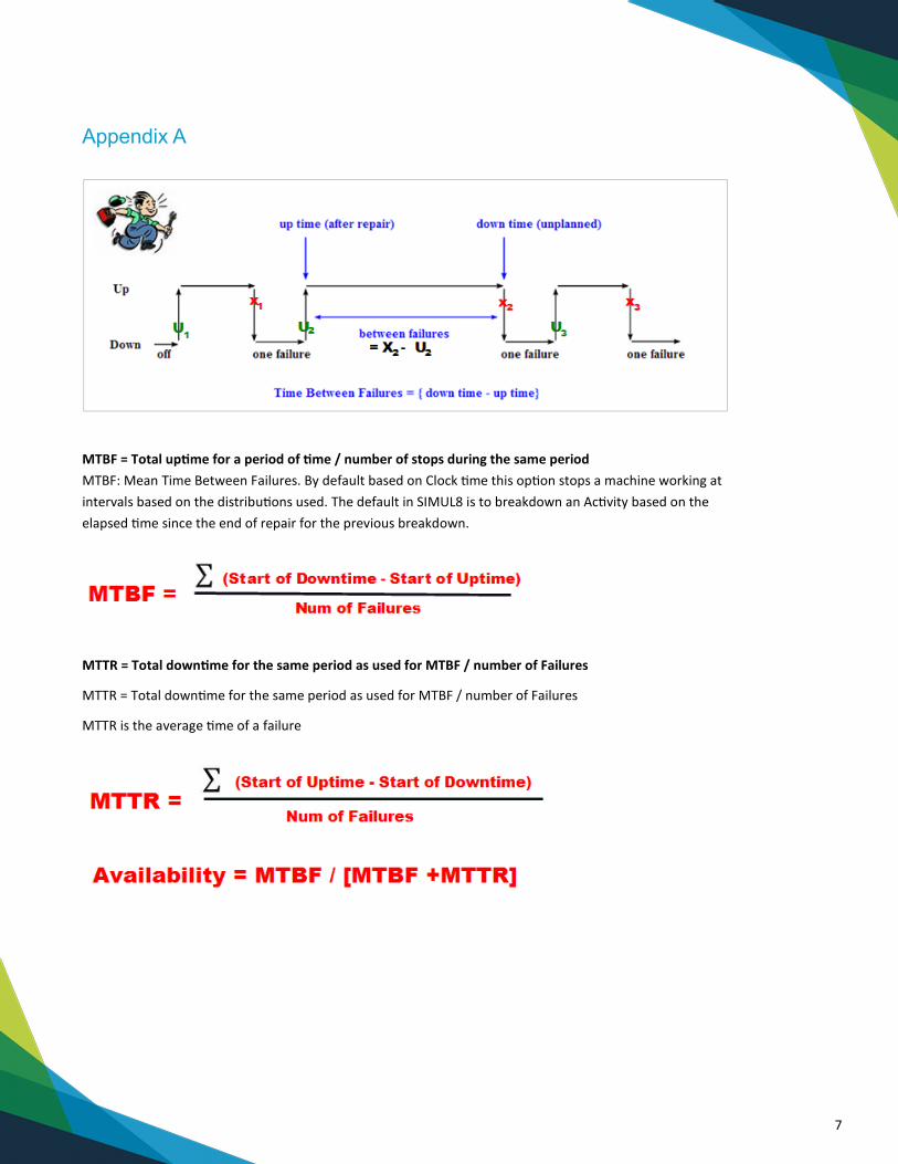
Appendix A

MTBF = Total uptime for a period of time / number of stops during the same period

MTBF: Mean Time Between Failures. By default based on Clock time this option stops a machine working at

intervals based on the distributions used. The default in SIMUL8 is to breakdown an Activity based on the

elapsed time since the end of repair for the previous breakdown.

MTTR = Total downtime for the same period as used for MTBF / number of Failures

MTTR = Total downtime for the same period as used for MTBF / number of Failures

MTTR is the average time of a failure