brexit and the impact of gradual economic integration on ...€¦ · brexit and the impact of...
TRANSCRIPT

Brexit and the impact of gradualeconomic integration on export
Rutger Teulings ∗
University of Amsterdam and Tinbergen Institute
July 27, 2017
Abstract
I develop an index for economic integration accounting for its gradual and bilat-
eral nature: the Gradual And Bilateral Integration (GABI) index. The graduality
captures differences in the depth and path of five stages in economic integration
and is an improvement over the use of binary dummy variables. Its bilateral na-
ture allows for country-pair differences, which is not possible with the multilateral
indexes in existing literature. I apply the GABI index to a gravity model for 18
OECD countries and estimate the impact of the five stages on export. The esti-
mates for these five stages allow me to investigate four different Brexit scenarios
in a general equilibrium analysis, ranging from soft to very hard Brexit. I find
that in the latter scenario real export of the UK decreases by a significant 32% in
the long run. Other EU countries also experience a decrease in real export, while
non-EU countries experience an increase due to trade diversion effects. Similarly,
I also investigate potential future free trade agreements like TTIP.
Key words: Balassa stages, economic integration, gravity model,
Brexit, TTIP.
JEL classification: F13; F14; F15.
∗Contact details. Address: Amsterdam School of Economics, PO Box 15867, 1001 NJ Amsterdam,The Netherlands; tel. +31-20-5254157; e-mail: [email protected] would like to thank Maurice Bun, Franc Klaassen and Yoto Yotov for their constructive feedback anduseful discussions helping to improve the paper. Furthermore, I would like to thank Ismael Valdes andAlfred Yong Chai Yee for their extensive work on the economic integration index.This paper is based on my MPhil thesis “The impact of gradual trade liberalization on export”.

1 Introduction
Economic integration is a time consuming process, it has a long path, and it differs in
depth across country-pairs. The most common way to estimate the effect of economic
integration agreements (EIA) on bilateral exports is by using bilateral dummy variables,
turning to one when economic integration commences and irrespective of how deep the
progress will go.
Dorrucci et al. (2005) has constructed a multilateral gradual integration index for
the EU-61, henceforth indicated by the ECB index. This index splits up EIAs into
smaller events. Each event is categorized into one of the five stages of economic in-
tegration, as defined by Balassa (1961), and gets weights assigned to based on the
contribution to the specific stage and total economic integration in general for all EU-6
countries combined. In this way it accounts for the depth and path of EIAs improv-
ing upon the binary dummy approach. However, the dummies are bilateral and can
account for differences in economic integration across country-pairs.
This paper proposes an alternative method. I construct a Gradual And Bilateral
Integration (GABI) index, based on the ECB index. The gradual aspects improves
upon the dummy variable and the bilateral aspect improves upon the ECB index. So,
I account for path and dept and differences across partners. The GABI index has
four advantages. First, the gradual aspect of the GABI index allows me to distinguish
the differences in depth and path of EIA. Second, it can identify all the different EIA
because the corresponding indexes reflect the differences in depth and path per EIA,
leading to more variation and less correlation between the respective variables. If one
captures all these EIAs by just adding more dummies they will start to overlap be-
cause they are only zero or one, potentially causing multicollinearity. Hence, dummy
variables cannot be added indefinitely to capture EIAs. This important property is
used to analyse the impact of Brexit later on. Third, the gradual aspect allows for the
identification of the dynamic impact of economic integration because lags no longer
also capture the gradual aspect of EIA. Finally, the bilateral aspect of the GABI in-
dex captures country-pair differences allowing me to use it as independent variable in
explaining bilateral exports, which is not possible with the multilateral ECB index.
There is a wide literature on the impact of economic integration on exports. Tin-
bergen (1962) is one of the first to study the impact of EIAs and in particular FTAs
on exports, by including among others an FTA dummy variable. He does not find a
significant effect. Today, the mainstream view in the economic literature is that eco-
1Belgium, France, Germany, Italy, Luxembourg and the Netherlands
2

nomic integration increases exports. In turn increasing exports increases GDP and
therefore welfare2. Among others, Baier & Bergstrand (2007), henceforth abbreviated
as BB2007, use a panel data model to show that bilateral exports of two FTA members
doubles after 10 years, where they use a dummy variable for countries that sign an FTA
and include lags to capture the phase-in. Roy (2010) distinguishes between an FTA
and a custom union (CU) dummy and finds that the CU is actually responsible for
the doubling of exports. Baier and Bergstrand further distinguish between 7 different
levels of economic integration in their multichotomous index (see Bergstrand’s website
http://www.nd.edu/jbergstr). Baier et al. (2014) use this index and find that economic
integration doubles trade and an FTA increases trade by 60%. Cipollina & Salvatici
(2010) show in their meta-analysis of 85 papers that the estimated impact on exports
of economic integration ranges between 12% and 285% a median of 46%. Dur et al.
(2014) have an extensive study of different type of economic integration agreements.
They remark the importance of the difference in depth of these agreements. They
develop a measure that varies between the integers 0 and 7. They also constructed
a similar measure using a latent trait analysis. Egger & Tarlea (2017) uses dummy
variables to capture different depths in FTAs. However, one cannot indefinitely add
dummies because this will lead to multicollinearity problems at some point. The GABI
index does not suffer from this problem.
As a framework for my empirical model I will use the extended real gravity model
by Klaassen & Teulings (2015a). The empirical model is applied to the export data of
18 OECD countries.
The empirical model is used to compare the estimated impact of dummy variables
capturing economic integration and GABI index. The results clearly display the two
advantages of using the GABI indexes over dummy variables, as discussed above. De-
pending on the estimation method, I find that aggregate of all five economic integration
stages increases exports between 35% and 108%.
Because it is now possible to obtain reliable estimates for the five different economic
integration stages using the GABI index, I can now use these estimates to evaluate
different Brexit scenarios, i.e. the UK leaving the EU. To that end I use a general
equilibrium (GE) analysis proposed by Anderson et al. (2015). The results show that
UK loses by far the most from Brexit in terms of exports, depending on the scenario
real exports decreases with 2− 32%, where the worst case scenario leads to the biggest
lose in exports. But also for other EU countries exports decreases as a consequence
2There are also disadvantages to economic integration, such as trade diversion. I will elaboratefurther on these disadvantages in Section 2.
3

of Brexit, especially Ireland for which real export decreases with 1 − 10%. Non-EU
countries mostly gain from Brexit, although the effects are small, due to the principle
of trade diversion, as proposed by Viner (1950), increasing real export with 0 − 1.2%.
In terms of real GDP it is not the UK that loses the most but Ireland, depending on
the scenario it loses between 0.4 − 1.4%.
The remainder of this paper is setup as follows. Section 2 discusses how to construct
the GABI index. Next, Section 3 shortly discuss the theoretical gravity model and use
it to justify the empirical model. The other data is described in Section 4. Section 5
displays the estimation results for the impact of the GABI indexes. The estimation
results are used in Section 6 to perform a GE analysis investigating different Brexit
scenarios, Transatlantic Trade and Investment Partnership (TTIP) and Comprehensive
Economic and Trade Agreement (CETA). In Section 7 I perform several robustness
checks. Finally, Section 8 concludes.
2 Economic integration
In this section I discuss the theoretical merits and costs of economic integration. Next,
I discuss the five stages of economic integration as proposed by Balassa (1961). Finally,
I explain how Dorrucci et al. (2005) construct the regional index based on these five
stages and how I extend and further improve this to the GABI index.
2.1 Theoretical views
Economic integration is when two or more countries are unifying economic policies, like
fiscal, trade, monetary, and social economic policies. The two extremes of economic
integration are autarky, no economic integration at all, and complete economic inte-
gration. In autarky a country is self-sufficient and has no access to other countries and
vice versa. Countries are completely integrated if they have full access to each other’s
markets. The motivation for economic integration can be both economical as well as
political.
The main economic motivation is to increase welfare in all participating countries
by allowing goods, services and production factors freely move between countries. This
is done by taking away both tariffs and non-tariff barriers (NTB), opening up foreign
markets and making trade worthwhile. Viner (1950) calls this trade creation and shows
that this by itself has a positive effect on welfare.
There are also other mechanisms that induces welfare gains from trade. The
Heckscher-Ohlin model (Heckscher (1919) and Ohlin (1933)) explain the gains from
4

trade with comparative advantage. A country has a comparative advantage in a cer-
tain good if it produces this good relatively more efficient than another country and
this leads to specialization. This leads to welfare gains. Rivera-Batiz & Romer (1991),
among others, argue that the opening up of foreign markets leads to larger markets.
Larger markets gives producers opportunity to expand leading to better economies of
scale, i.e. lower average cost per unit produced, and therefore a rise in welfare. On
a micro level, Melitz (2003) shows that intra industry trade leads to a reallocation
of resources to the more productive firms. This reallocation increases the aggregate
industry productivity, leading to a welfare gain.
The main political motivation is that economic integration is considered to be the
first step to a stable political union. For example, in 1951 the European Coal and Steel
Community (ECSC), the predecessor of the EU, was founded. The main goal of the
ECSC was preventing any future wars, like world war I and II, from happening again in
Europe by enforcing cooperation in the two most important resources for the defence
industry.
However, economic integration between countries also has its drawbacks. The re-
duction of trade barriers among participating countries and possibly implementing com-
mon trade barriers towards non-participating countries leads to trade diversion (Viner
(1950)). Trade diversion occurs when two countries, say, the Netherlands and Ger-
many, liberalize trade. As a consequence it might become cheaper for the Netherlands
to import a good, say, cars from Germany instead of importing it from a third more
efficiently car-producing non-participating country. Hence, the more efficient indus-
try loses market share to a less efficient industry leading to a decrease in the formers
welfare. At the same time the Netherlands receives less income from import tariffs
reducing its welfare.
Second, trade creation can lead to unemployment in the country with the relatively
least productive industry, because this industry might be forced to close down due
to increasing competition. Viner (1950) shows that trade creation is overall welfare
increasing, but there are countries that gain and countries that lose from trade creation
and only by redistributing the welfare gain it can be ensured that all countries gain
from trade creation. In practice this is often difficult to realize, offering an important
argument for protectionism, i.e. refraining from (further) economic integration.
Finally, the currently most topical drawback of economic integration is that the
bigger the depth of economic integration, the more sovereignty, concerning legislation,
monetary and fiscal policy et cetera, the individual countries lose. Recently, this has
lead to increasing economic and political tension in the EU, giving rise to strong anti-EU
5

movements in almost all EU member states.
2.2 The Balassa stages
Balassa (1961) divides economic integration into five stages, henceforth called Balassa
stages, where each subsequent stage is deepening the integration; so the stages are
cumulative. For example, if a group of countries reached stage 2 they automatically
reached stage 1 as well. The Balassa stages are:
FTA Free trade agreement: all member states abolish trade tariffs and import quotas
for goods and services with respect to other member states. Each member state
maintains its own trade barrier policies regarding non-member states. NTBs can
still prevent perfect free trade.
CU Custom union: an FTA, where in addition all members have uniform trade barrier
policies regarding non-member states.
CM Common market: a CU, where all other NTBs on export and restrictions on
factor movements between member states are abandoned and a common policy
regarding non-member states.
EUN Economic union: a CM, with advanced cooperation concerning economic policies
and standardization of relevant national laws.
TEI Total economic integration: a EUN, where all relevant economic policies, such as
monetary and fiscal policies, are arranged at a supranational level. To enforce
these policies supranational authorities and laws are installed.
2.2.1 Application to the EU
The EU’s economic integration history is a good example for the Balassa stages. In 1951
the EU-6 signed the treaty of Paris founding the European Coal and Steal Community
(ECSC). In 1957 the ECSC was extended with the rectification of the treaty of Rome.
This added, next to the political goal of peace and stability, the economic goal of trade
liberalization. In 1968 both the FTA and CU were completed.
In the Schengen Agreement in 1985, the member states agreed to abolish all borders
between the participating countries. Although the actual implementation is more than
10 years later. With the Single European Act (SEA) in 1986 the member states agreed
to reach a single market by the end of 1992, further abolishing NTBs. These two
6

agreements were a major step towards a CM. In the same period the EU was extended
with new members. Table C.1 displays all the EU-153 entry dates.
The foundations for an EUN were already laid down with the treaty of Rome,
starting to unify national laws and economic policies. Over time this was developed
further. The treaty of Maastricht in 1992 arranged, among others, a staged plan towards
a single currency and further unified national laws, economic and monetary policies, an
important step towards EUN and TEI. In 1999 the Euro became the common currency
in eleven EU countries4. Greece joined in 2001.
In the next 12 years the treaty of Amsterdam, Nice and Lisbon were signed to
reform the EU’s institutional structure contributing further to TEI and making future
extension of its members possible, especially towards Eastern Europe.
Important future steps towards TEI are: more labor mobility, extending unification
of the European capital market and aligning national structural and macroeconomic
policies.
2.3 Constructing the Gradual And Bilateral Integration index
I use the constructed ECB index by Dorrucci et al. (2005) to construct a Gradual And
Bilateral Integration (GABI) index that measures the depth and path of economic in-
tegration. First, I describe how the ECB index is constructed and measure multilateral
economic integration in the EU-15. Next, I explain how I extend this data set and how
I use it to create a bilateral GABI index.
2.3.1 The ECB index: multilateral economic integration
Dorrucci et al. (2002) construct the multilateral ECB index from 1957-2001 for the
EU-6 as a whole. Later on Dorrucci et al. (2005) specify the multilateral economic
integration for each of the EU-6 separately and extend the data-set by including the
remaining EU-15 countries. This partly involves the development within the EFTA
and EEA.5
3This are all EU countries before the May 2004 expansion: Belgium, France, Germany, Italy, Lux-embourg, Netherlands, Denmark, Ireland, United Kingdom, Greece, Portugal, Spain, Austria, Finlandand Sweden.
4Belgium, France, Germany, Italy, Luxembourg, Netherlands, Ireland, Portugal, Spain, Austria andFinland.
5Dorrucci et al. (2015) append the regional index by including the development and changes of theEconomic and Monetary Union (EMU) as a consequence of the financial and euro area crisis. This newindex allows for even deeper economic integration. However, since my data only goes up to 2011 I willrefrain from using this updated index.
7

The main idea of the multilateral ECB index is to divide the complete economic
integration into smaller events. Subsequently, each event is categorized into one of the
five Balassa stages and gets points assigned representing its contribution to the specific
stage. Events only receive points if they implement an EIA, while only signing a new
agreement to implement new EIA in the future gets zero points. For example, the
initial Schengen agreement is signed in 1985, while the actual abolishment of border
controls becomes only affective in 1995. Therefore, the former gets 0 points and the
latter gets 1 point.
Together all events in a Balassa stage have a maximum of 25 points, with the
exception of the FTA and CU stages, they get assigned 15 and 10 points, respectively.
So, countries that complete economic integration get 100 points, while countries in
autarky get 0 points. The point distribution for each of the five stages is only given
for the EU-6 as a hole. For all the 15 countries separately, they only report the total
number of points for all stages combined.
The assigning of points to different events allows for the distinction in the difference
of depth and path in EIA. Still, the distribution of points is subjective, regarding both
the number of points for a single event as well as the distribution of points over the five
stages. For some measures, like the abolishing of trade tariffs, the assigning of points
can be done in a relative objective way because tariffs are reduced in percentages and
the reduction steps are therefore comparable. For other more abstract measures, like
abolishing border controls, it is hard to define their individual contribution and mutu-
ally compare their contribution. However, dummy variables are even more subjective
because they capture EIA with different depths and paths with a binary variable. The
researcher has to determine when he lets the dummy variable switch to one, at the
beginning, halfway or at the end of reaching, say, a FTA and whether he treats all EIA
identical, even though they vary in depth and path, or that he leaves out the more
shallow EIA.
The contribution of the ECB index is twofold. First, it allows for the comparison
of the difference in depth and path of economic integration between different regions
and Balassa stages, while binary dummy variables do not allow for this distinction.
Second, it allows for the identification of the impact of EIA between different regions,
Balassa stages and the dynamic impact of EIA, while binary dummy variable cannot
identify all these different aspects at the same time because the largely overlap causing
potential multicollinearity problems between the different dummy variables. The ECB
index has one disadvantage, it is time consuming to construct compared to a dummy
variable.
8
The five stages in the ECB index can develop in parallel, that is opposite to the
Balassa stage, where the stages develop in progressive order. Furthermore, The stages
in the ECB index measure only the additional contribution to economic integration,
whereas the Balassa stages are cumulative. I indicate the additive nature of the stages
with a + in the superscript.
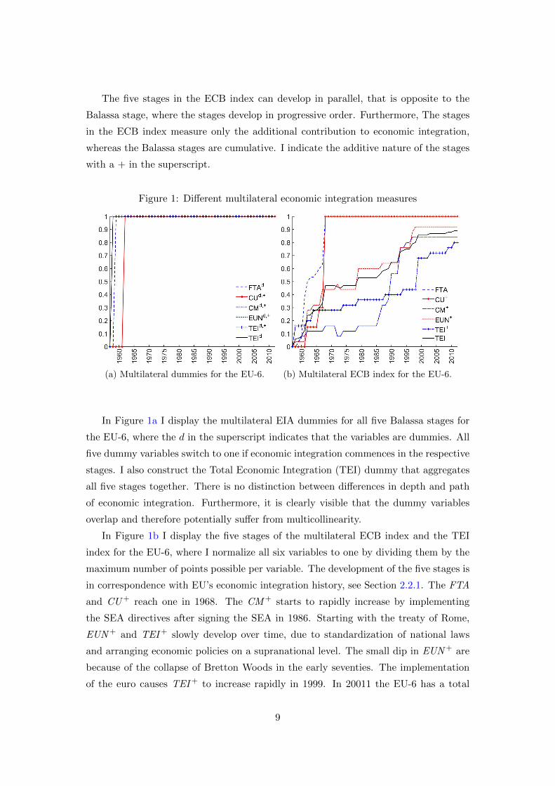
Figure 1: Different multilateral economic integration measures
(a) Multilateral dummies for the EU-6. (b) Multilateral ECB index for the EU-6.
In Figure 1a I display the multilateral EIA dummies for all five Balassa stages for
the EU-6, where the d in the superscript indicates that the variables are dummies. All
five dummy variables switch to one if economic integration commences in the respective
stages. I also construct the Total Economic Integration (TEI) dummy that aggregates
all five stages together. There is no distinction between differences in depth and path
of economic integration. Furthermore, it is clearly visible that the dummy variables
overlap and therefore potentially suffer from multicollinearity.
In Figure 1b I display the five stages of the multilateral ECB index and the TEI
index for the EU-6, where I normalize all six variables to one by dividing them by the
maximum number of points possible per variable. The development of the five stages is
in correspondence with EU’s economic integration history, see Section 2.2.1. The FTA
and CU + reach one in 1968. The CM + starts to rapidly increase by implementing
the SEA directives after signing the SEA in 1986. Starting with the treaty of Rome,
EUN + and TEI + slowly develop over time, due to standardization of national laws
and arranging economic policies on a supranational level. The small dip in EUN + are
because of the collapse of Bretton Woods in the early seventies. The implementation
of the euro causes TEI + to increase rapidly in 1999. In 20011 the EU-6 has a total
9

of 89 points out of 100. The two advantages of the regional index are clearly visible,
comparing it to the dummy variables. It is possible to have different depths and paths
of economic integration and to identify the five stages separately.
2.3.2 Extending the ECB index
The ECB index is updated and extended by me in three ways. First, based on the
original treaties6 I determine for each EU-15 country separately to which of the five
stages their points must be assigned, similar to the EU-6 as a whole in Dorrucci et al.
(2005). Hereby, I use their proposed distribution of points over the five stages.7
Second, I extend the data-set to 2011 and update and extend the events based on
the original treaties, making the accession of, say, Greece to the EU even more gradual.
Finally, I extend the data set by including the separate multilateral development of
CUSFTA and NAFTA, where I include the CUSFTA countries Canada and the USA,
and I include two additional EFTA members Norway and Switzerland and.8 Japan is
also added to the data set but no EIA is assigned to Japan with respect to any other
countries in the data set.9
Future extensions of the ECB index can be to include even more details of all the
EIA making it even more gradual, extend the ECB index to incorporate other countries
and including multilateral treaties such as the General Agreement on Tariffs and Trade
(GATT). We will leave this for future research.
2.3.3 The GABI index: bilateral economic integration
To construct the GABI index from the extended multilateral ECB index I have to take
into account that a country can sign an EIA with respect to a different set of countries.
For example, if in 1959 the UK joins the EFTA it engage in economic integration with
respect to all EFTA members, but when in 1973 the UK joins the EU-6 it engage in
economic integration with respect to the EU-6. So, I cannot simply add these two EIA
to obtain UK’s total economic integration, because the EIAs are signed with respect
to two different set of countries. So, I have to keep track with respect to what set of
countries a country signs an EIA. Furthermore, it is not enough to simply keep track of
which countries join the EU. For each EIA event one has to keep track which country
6http://eur-lex.europa.eu contains the different accession treaties of new member-states.7see Table A1.1 and A1.2 in their appendix for an extensive description8The newly added events are constructed with information from various sources, such as the EU,
EFTA, EEA, World Trade Organization, International Monetary Funds (IMF), Ministries of Trade andInternational Labor organizations.
9The FTA, signed in 2010, between Japan and Switzerland is not jet incorporated in the ECB index.
10

signed it and which did not taking into account that countries can enter or leave at
a later period in time. For example, when Greece enters the EU in 1981 it does not
join the European Monetary System (EMS). So, when Spain joins the EMS in 1989 it
does not get points with respect to Greece, even though Greece entered the EU like
Spain. Only when Greece enters the EMS in 1998, Greece gets the assigned points with
respect to all other EMS countries. By careful bookkeeping we can construct a GABI
index.
Figure 2: Total economic integration: multilateral versus bilateral
(a) Multilateral TEI of the EU-6. (b) Bilateral TEI ijt for Germany i-j.
To exemplify the importance to go from unilateral to bilateral, I compare Figure
2a with Figure 2b. The former displays the multilateral TEI of the EU-6 in, the
same as that in Figure 1b. The latter displays TEI ijt between Germany and five
different countries: France (FR), Greece (GR), United Kingdom (UK), Sweden (SD)
and Switzerland (SW), where again all five TEI ijt are normalized by dividing them
by the maximum number of points (100). By making the ECB index bilateral, each
country-pair has a different depth and path of TEI ijt, while the multilateral ECB index
can only capture TEI for the EU-6 as a whole. Not only is this possible for TEI ijt, the
aggregate of the five Balassa stages, but for all five Balassa stages separately as well.
If I capture the five TEI ijt series in Figure 2b with dummy variables, I can no
longer distinghuis between the differences in depth and path between the country-
pairs. Furthermore, I have to make a subjective choice when the dummy switches to
one. For example, at the beginning of economic integration or after passing a certain
threshold. If I chose, say, the former then I will not be able to distinguish the country-
pairs BD-SD from BD-SW and BD-UK will also be very similar. This exemplifies the
11

advantages of the GABI index over bilateral dummy variables.
3 Empirical approach
In this section I will shortly describe the theoretical gravity model that I use both as a
starting point for my empirical model, that I describe next, and in the GE analysis of
Brexit, TTIP and CETA. Finally, I elaborate on the estimation method.
3.1 The theoretical gravity model
The gravity model explains bilateral export with the basic idea that the larger two
countries are in economic terms the more they trade, where economic size is measured
by GDP. However, the further two countries are apart the less they trade. This can
be both physical and economic distance, for instance high bilateral tariff rate between
two countries. This is called the bilateral trade barrier.
Tinbergen (1962) is one of the first to use the gravity model to analyze trade flows,
since that time the model is used as a workhorse model in trade literature. Although its
theoretical motivation was missing in the beginning, its explanatory power was evident.
Anderson (1979) and Bergstrand (1985) are one of the first who give a theoretical
justification for the gravity model. Recently Anderson & van Wincoop (2003) make an
important contribution. They introduce the notion of multilateral export and import
resistance, measuring the weighted resistance to export and import respectively. Now
it is the bilateral trade barrier relative to the weighted trade barrier with respect to
the rest of the world (RoW) that matters for bilateral export and not only the bilateral
trade barrier itself. For example, if the RoW is relatively far away from these two
countries, then it becomes for them relatively cheaper to import from each other than
from the RoW. This paper gave a boost to the theoretical gravity literature and since
then various extensions and new insights are published.
In this paper I will use a recent extension by Klaassen & Teulings (2015a). They
introduce the exchange rate into the nominal gravity model and show how to rewrite this
into a real gravity model. Introducing the exchange rate has three advantages. First,
the exchange rate is important in explaining export. If the currency of the exporter
decreases, its goods become cheaper for the importing country leading to more exports.
Second, it also introduces the effective exchange rate of both the exporter and importer
through the multilateral resistance (MR) terms. If the effective exchange rate of, say,
the exporter depreciates vis-a-vis the RoW its good becomes cheaper for the RoW
leading to more demand and thus higher prices for its good. This crowds out import
12
from the importer. Finally, the exchange rate ensures that the currency dimensions on
both the left- and right-hand-side are the same.
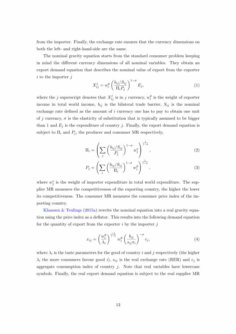
The nominal gravity equation starts from the standard consumer problem keeping
in mind the different currency dimensions of all nominal variables. They obtain an
export demand equation that describes the nominal value of export from the exporter
i to the importer j
Xjij = wyi
(bij/SijΠiPj
)1−σEj , (1)
where the j superscript denotes that Xjij is in j currency, wyi is the weight of exporter
income in total world income, bij is the bilateral trade barrier, Sij is the nominal
exchange rate defined as the amount of i currency one has to pay to obtain one unit
of j currency, σ is the elasticity of substitution that is typically assumed to be bigger
than 1 and Ej is the expenditure of country j. Finally, the export demand equation is
subject to Πi and Pj , the producer and consumer MR respectively,
Πi =
∑j
(bij/SijPj
)1−σwej
11−σ
, (2)
Pj =
(∑i
(bij/Sij
Πi
)1−σwyi
) 11−σ
, (3)
where wej is the weight of importer expenditure in total world expenditure. The sup-
plier MR measures the competitiveness of the exporting country, the higher the lower
its competitiveness. The consumer MR measures the consumer price index of the im-
porting country.
Klaassen & Teulings (2015a) rewrite the nominal equation into a real gravity equa-
tion using the price index as a deflator. This results into the following demand equation
for the quantity of export from the exporter i by the importer j
xij =
(wyiλi
) −11−σ
wyi
(bijsijπi
)−σcj , (4)
where λi is the taste parameters for the good of country i and j respectively (the higher
λi the more consumers favour good i), sij is the real exchange rate (RER) and cj is
aggregate consumption index of country j. Note that real variables have lowercase
symbols. Finally, the real export demand equation is subject to the real supplier MR
13

of country i πi
πi =
∑j
(bijsij
)1−σwej
11−σ
, (5)
where πj is similar to πi and wxji is the weight of bilateral export of country j to i in
total export by country j.
There are two striking difference between the real and the nominal model. The first
difference is the additional term on the right-hand-side(wyiλi
) −11−σ
. If the taste parameter
of good i increases, good i becomes more popular in the RoW increasing the price for
good i. Consequently, country j can consume less of good i. If the weighted output
of country i increases, good i is supplied more abundant decreasing the price for good
i. Consequently, country j can consume more of good i. The second difference is that
the consumer price index of the importer no longer plays a role.
3.2 The empirical model and estimation
I will use a three dimensional FE panel data model approach to model the real gravity
equation in (4), where I include a time dimension t as the additional third dimension.
BB2007 and Egger (2000) show that FE are preferred over random effects. Just as
Klaassen & Teulings (2015a) I will consider a log-linearized version of the real gravity
model (4) subject to (5). I will add multiple FE-types to capture most source of
unobserved heterogeneity. To prevent multicollinearity between all these FE-types, I
use the untangling normalization method as introduced in Klaassen & Teulings (2015b)
and as extended to a three dimensional panel data model in Klaassen & Teulings
(2015a). Hence, the benchmark empirical model becomes
expijt = GABI ′ijtβ+α+αxi +αmj +αij+τ ·t+τxi ·t+τmj ·t+τij ·t+θt+θxit+θmjt+εijt, (6)
where expijt is the log of real export from country i to j at time t and our main
independent variable GABI ijt with KGABI variables based on the GABI index. I
assume that all variables are uncorrelated with the error term. See Section 3.2.1 for
a more extensive discussion on this. I assume that the error term εijt is not cross-
sectionally correlated and I allow it to be heteroscedastic and serially correlated.
The GABI index is part of the bilateral trade barrier and varies over three di-
mensions. However, the bilateral trade barrier consists also of many different country
and country-pair specific characteristics, for example being landlocked and a common
language, respectively. Therefore, I will add exporter and importer FE, αxi αmj and
14

country-pair FE αij . Finally, I will also add an overall constant α.
Exporter τxi · t and importer trend FE τmj · t and country-pair trend FE τij · tare included, as proposed by Bun & Klaassen (2007). They show that trends in the
residuals, due to omitted variables, will lead to biased estimators, because the variables
partly pick up the trending behavior in the residuals. Finally, we also add an overall
trend τ · t as is common in the time-series literature.
Time FE θt are included to capture for example the development of world income
over time. Trade is affected by alternating periods of economic growth and economic
crises, such as the oil (1973) and financial crisis (2008).
Finally, I will use the exporter-time θxit and importer-time θmjt FE to capture all
variables that only vary over the exporter and time or the importer and time, e.g
both MR terms and the RER10, but also unobserved exporter-time and importer-time
heterogeneity. For my research question it does not matter that by adding country-time
FE the impact of these variables is not identified, as my focus is on GABI ijt and the
former is not multicollinear with the latter. While Anderson & van Wincoop (2003)
show that ignoring the MR terms leads to substantial biases. Fally (2015) shows that
the use of country FE in a cross-sectional analysis to capture the MR terms is consistent
with the structural approach of Anderson & van Wincoop (2003) and Egger & Larch
(2012) argue that the later actually leads to inconsistent estimates due to unobserved
country specific effects. The additional time dimension in my analysis implies that
country-time FE become the equivalent of country FE in a cross-section.
To estimate (6), I will use LSDV. One other commonly used method to estimate
gravity models is PPML, as proposed by Santos-Silva & Tenreyro (2006). This approach
has two main advantages. First, this approach is that it can deal with zero trade flows in
the data. However, there are no zero trade flows for the countries in my sample; so this
advantages plays no role of importance in this paper. Second, if one include exporter
and importer FE in PPML, the sum of the estimated trade flows per exporting and per
importing country equals the sum of the true value of the trade flows per exporting and
importing country respectively, see Fally (2015) and Arvis & Shepherd (2013), where
LSDV will consistently overestimates the sum of the true values per exporting or per
importing country due to Jensen’s-inequality. This nice property is important in our
general equilibrium analysis, see Section 6. Therefore, I will also estimate the gravity
model using PPML. In that case (6) the right-hand-side changes into an exponential
model and the dependent variable is in levels.
10Even though RER is an ijt variable it is multicollinear with a linear combination of exporter-timeand importer-time dummies because RERijt = RERiUSt − RERjUSt; so RERijt can be written as alinear combination of it and jt variables.
15

Throughout the paper I will use Newey-West standard errors with 3 lags11 (see
Newey & West (1987, 1994)) to correct for heteroscedasticity and serial-correlation in
εijt. I use a 5% significance level throughout the paper.
3.2.1 Endogeneity
One potential source of endogeneity is due to omitted variables. The broad range of FE-
types included in to the model capture different sources of unobserved characteristics,
such as country(-pair), country-(pair) trend, time and country-time characteristics pre-
venting an omitted variable bias in the GABI estimates. Even non-linear characteristics
can potentially be partly captured by the wide range of FE-types.
Simultaneity is another potential source for endogeneity. There are two potential
causes of simultaneity. First, exports has a positive effect on GDP so that GDP is
endogenous. However, I look at bilateral exports and GDP and therefore, because
the former is often small compared to the latter, the simultaneity effect is typically
neglected. This is supported by Frankel (1997). This argument does not hold for
intranational export flows. These are often between 70 − 60% of GDP. However, the
share of intranational exports with respect to GDP is very constant over time or has a
constant trend. Indeed, plots of these demeaned and detrended shares show that most
fluctuation is within 2%. So, the inclusion of country and country trend FE might
substantially mitigates endogeneity in this case. The second source of simultaneity
is that high or relatively fast increasing exports between country-pairs can induce an
FTA. BB2007 uses country-pair FE to capture the level and Bun & Klaassen (2007)
additionally include country-pair trend FE to capture the trend, together resolving this
simultaneity problem to a large extent.
Finally, the third source is measurement error. In particular the GABI index is
prone to measurement error. However, changing the EIA dummy variable into a GABI
index will only decrease the measurement error, because it becomes more realistic. So,
most likely the potential bias due to measurement errors in the economic integration
variable will be reduced compared to using an EIA dummy.
To analyse whether endogeneity is not biasing the estimates, one can perform an
IV regression. The literature offers many examples of such analysis. Bun & Klaassen
(2007) perform an IV regression using one period lagged FTA and Euro dummies as
instruments and find that this did not lead to significantly different estimates. So, given
that I use a similar model specification, I conclude that there is no indication that I
need to worry about endogeneity in this paper.
11The number of lags is selected by calculating 4 ∗ (T/100)2/9 and rounding it down.
16
4 Data
In this research I use 18 countries. I include all EU-15 countries excluding Belgium and
Luxembourg12, Canada (CN), Japan (JP), Norway (NW), the United States (US) and
Switzerland (SW). I include intranational export flows, export from country i to i, so I
have 324 country-pairs. The data ranges from 1965-2011 (T = 47) resulting into 15228
observations. Economic integration for the EU already starts in 1957, especially in the
first two Balassa stages, so I need to let the data start as early as possible. However,
data availability in general and the poor quality of the bilateral export data in the early
60s forces us to choose our starting data not earlier than 1965.
For export flows from country i to j I use monthly nominal export data in US dollars
from the IMF Direction Of Trade Statistics (DOTS) and convert it to exporter countries
currency with the exchange rate from the International Financial Statistics (IFS) of the
IMF. Next, I calculate yearly averages. To obtain real export I divide the obtained series
by the exporter price index from AMECO of the European Commission. Finally, to
ensure common scaling in real US dollars I divide by the purchasing power parity (PPP)
of the US dollar in i currency obtained from the OECD Economic Outlook, where we
use the base year 2010 because all other indexes use the same base year.
To construct intranational export flows I take the total trade flows from country i
to the world from DOTS and transform it from US dollars with the exchange rate from
the IFS into i currency. Next, I subtract this series from yearly nominal GDP obtained
from AMECO, where I use the exchange rate from AMECO to denominate the latter
in i currency. To obtain real trade flows I use the same approach as before.
To be able to compare our GABI index with a binary FTA dummy, used standardly
in the literature, we construct FTABBijt based on BB2007. Table C.1 (Appendix C)
displays all the different FTAs we take into account and all members’ entry and exit
dates.
We also created economic integration dummies based on our own GABI index. For
each stage we construct a binary variant that equals one if the corresponding stage
in the GABI index is non-zero, otherwise the binary variable is zero. These binary
economic integration dummy variables are indicated with a d in the superscript.
The remaining variables are the same as in Klaassen & Teulings (2015b) and I refer
to their data description for further information.
12Austria (OE), Denmark (DK), Finland (FN), France (FR), Germany (BD), Greece (GR), Ireland(IR), Italy (IT), the Netherlands (NL), Portugal (PT), Spain (ES), Sweden (SD), United Kingdom(UK).
17

5 Results
In this section I will analyze the results of estimating the impact of the GABI index.
First, I will focus on the first Balassa stage and explore the difference between the
GABI and the dummy variable to estimate the effect of an FTA. Next, I will discuss
the estimation results of all five Balassa stage. Throughout this section I will omit the
ijt subscript for brevity.
5.1 Free trade agreements
Table 1: Estimated impact of FTA based on different FTA variable definitions
Lags of FTA No Yes
No. of lags – – – 11 11 7
FTA variable FTABB FTAd FTA FTABB FTAd FTA
FTA 0.16 * 0.09 * 0.19 * 0.38 * 0.45 * 0.26 *(0.02) (0.02) (0.03) (0.04) (0.04) (0.04)
The dependent variable is expijt. For the three models with lags of the FTA variable I onlyreport the overall effect. Standard errors are between brackets. * indicates significance at5% level.
To be able to compare GABI index with the use of binary dummy variables I
estimate the impact of an FTA using three different specifications. The dummy variable
FTABB is based on an FTA dummy variable used by BB2007 (see Section 4), FTA is
the first stage of the GABI index, so a gradual variable, and the dummy variable FTAd
is 1 if FTA is non-zero. For a more extensive description of the latter two see also
Section 2.3.
In Table 1 in the first three columns I display the estimation results for the static
model. The estimation results for FTABB and FTA are similar. However, the FTAd
estimate is considerably smaller than both estimates. This is remarkable, especially
because FTAd and FTABB are very similar being both dummy variables. The difference
between these two variables is purely that FTABB does not take into account two
association agreements; Finland becomes associate EFTA member in 1961 and Greece
signs an association agreement with the EU-6 in 1962. In the GABI index these two
association agreements get both 2 points out of the possible 15, but the FTAd variable
cannot distinguish between a full and shallow FTA. So here it is better to omit shallow
FTAs. However, when is an FTA shallow and when is it full? This a subjective and
not so obvious choice that one has to make and the results show that it can influence
the estimates quite heavily.
18

The estimated impact of FTA is 0.19 implying a ([exp(0.19) − 1] ∗ 100 =) 21% in-
crease in exports. Similarly, the estimated impact of FTABB is 0.16.
This effect is considerably smaller than the estimated impact of 0.46 by BB2007
in a similar model (see BB2007 Table 5 p. 89). This can mostly be explained by my
inclusion of τij · t (Section 7.2 confirms and further explain their importance). If I do
not include τij · t I find an estimated impact of 0.51 for FTABB (not shown).
Next, I will incorporate lags of the FTA variable to take dynamic FTA effects into
account. The number of lags is based on significance. Possible dynamic effects are
habit formation of consumers and exporters and importers that need time to adjust to
the opening up of new markets due to a new FTA treaty. Besides the level effect I will
add (lagged) first differences to capture the dynamic component, such that the former
still captures the long-term effect and they are still comparable to the static estimates.
BB2007 also include lags in on of their model specification to model the time it
takes to actually reduce tariffs after the introduction of an FTA, so called phase-in.
However, the GABI index already captures this effects ensuring that including dynamics
only captures the lagged response of consumers, exporters and importers on an FTA.
So, the GABI index disentangles the phase-in dynamics from the actual dynamics on
exports.
The last three columns in Table 1 display the result when including dynamics. For
the GABI index variable I need to include seven lags indicating that it takes seven
years before consumers, exporters and importer fully adjust to the new FTA. As a
consequence the FTA effect increases to 0.26. For FTABB I need to include 11 lags,
substantially longer than for the FTA variable. BB2007 show that they need to include
10 year lags.13 Hence, due to the need to capture the phase-in one need to include
more lags for FTABB. The same holds for FTAd.
The estimated impact of both dummy FTA variables is substantially larger than
that of FTA. Still, the estimated impact for FTABB of 0.38, a 44% increase in exports,
is a lot smaller than the doubling found by BB2007 when including phase-in effects;
they find an increase in exports of 114%. This difference is again almost completely
explained by the addition of τij · t, omitting τij · t leads to an increase of 97% in exports
(not shown).
Summarizing, I show that including shallow FTAs in a dummy variable influences
the estimated impact. However, the researcher has to make a subjective decision when
an FTA is shallow and should therefore be omitted. The GABI index allows us to distin-
13They use data with a five year interval, so they only include two lags. However, this implies thatthe Phase-In period is 10 years.
19

guish between the depths of different FTAs and therefore circumventing this problem.
Furthermore, I show that the gradual aspect of the GABI index allows me to no longer
use FTA lags to capture the phase-in. Instead, the lags now solely capture the dynamic
impact of an FTA.
5.2 All stages in the GABI index
Table 2: Estimated impact of the GABI index using different model specifications
Incremental Balassa stages Aggregate Balassa stages
Description GABI Dum. GABI GABI, PPML GABI Dum. GABI GABI, PPML
FTA 0.06 * 0.14 * 0.24 *(0.02) (0.03) (0.06)
CU+ 0.19 * 0.17 * 0.22 *(0.05) (0.04) (0.04)
CM+ −0.11 −0.27 * −0.28 *(0.09) (0.06) (0.05)
EUN+ 0.01 0.03 0.18 *(0.03) (0.08) (0.06)
TEI+ 0.15 0.29 * 0.36 *(0.10) (0.14) (0.11)
TEI 0.08 * 0.47 * 0.65 *(0.02) (0.05) (0.07)∑
GABI 0.30 * 0.36 * 0.73 * – – –(0.03) (0.08) (0.09)
The dependent variable is expijt. All models are estimated with LSDV unless described otherwise.The inclusion of dynamics is not displayed. Using LSDV, only FTA has 7 significant lags (see Table1). The estimated FTA impact becomes 0.22 (0.04) and the estimated
∑GABI becomes 0.45
(0.09). All other estimates hardly change. Using PPML, both FTA and CU+ have 5 significantlags. The estimated impact of FTA hardly changes and that of CU+ becomes 0.33 (0.05). Theestimated
∑GABI becomes 0.85 (0.11). All other estimates hardly change. Standard errors are
between brackets. * indicates significance at 5% level.
In this section I will consider all five Balassa stages. In the first two columns I
estimate the impact of all five Balassa stages using dummy variables based on the
GABI index and the GABI index itself, respectively. In the third column I reestimate
the latter model using PPML instead of LSDV. Finally, I repeat this comparison in
column four to six using the TEI variable that aggregates all five stages. See Section
2.3 for a more extensive description of the variables.
The estimated FTA impact in column two is 0.14, that is a slight decrease compared
to Table 1. The decrease is possibly explained by the fact that FTA and CU + develop
rather similar. Therefore, estimating a model with only FTA will cause it to partly
capture the impact of CU +.14
14If I omit CU+, the estimated FTA impact increases to 0.17, close to the estimate in Table 1supporting this argumentation.
20

The estimated impact of CU + is 0.17. Hence, a CU , combining the first two Balassa
stages, has a significant estimated impact of 0.31. This is in line with Roy (2010), who
estimate that the impact of a CU is bigger than that of an FTA.
The third stage, CM +, is the only of the five stages that has a negative effect on
exports. I find an estimated impact of -0.27. This result may seems strange at first
glance, that is, more integration reduces exports. However, it might actually sheds new
light on the discussion of the relation between free factor movements, specifically that
of capital, and exports. There is an ongoing debate about the tradeoff between export
and foreign direct investment (FDI). If the cost of factor movement decreases it might
be bettor for firms to engage in FDI to serve the local market instead of exporting,
explaining a negative CM + effect. This is the so called proximity versus concentration
trade-off. Among others Brainard (1997) finds empirical support for this tradeoff.
Helpman et al. (2004) shows that the most productive firms engage into FDI and the
second most productive firms engage in export. A CM makes FDI easier, lowering the
threshold for less productive firms to engage in FDI and therefore reducing the average
productivity of exporting firms. So, my results show that CM + favours proximity over
concentration.
The estimated impact of EUN + is not significant. The fact that standardization of
relevant national laws and integration of economic policies does not have a big effect on
exports when a CM market is already realized seems plausible. This estimate is also in
line with Bun & Klaassen (2007) who find that the Euro only lead to a small increase
in exports, realizing that the introduction of the euro mainly leads to an increase of
EUN +. Another potential cause for the insignificant estimate is that EUN + and TEI +
are highly correlated leading to a collinearity problem. This is supported by the fact
that omitting TEI + leads to a significant estimated impact of EUN +.
The estimated impact of TEI + is 0.29. This is the largest contribution to an increase
in exports of all five stages implying that arranging policies at a supranational level
leads to the most additional gains in exports.
If I sum all estimated impact of the five stages I find that the total significant impact
on economic integration is 0.36, this leads to a 43% increase in exports. This is very
close to the median of 46% found by Cipollina & Salvatici (2010) in their meta-analysis,
but only half of their mean of 80%.
In column five I estimate the impact of TEI to be 0.47, implying a 60% increase
in exports. This is between the median and mean of the meta-analysis by Cipollina &
Salvatici (2010).
In general the model with dummy variables in column one results into mainly in-
21

significant estimates. A likely cause for this can be the high multicollinearity between
the five dummy variables because these variables cannot disentangle country-pair spe-
cific differences in the depth and path of economic integration (for example see Figure
1a). Only the estimated impacts of the dummy variables for FTA and CU + are sig-
nificant, because the dummy variables of different stages are very similar leading to
no or weak identification of the estimated impact of the five stages. The FTA dummy
variable estimate is still considerably smaller than its GABI index counterpart, while
that of CU + is similar to its GABI index counterpart. The sum of estimated impact
of the five stages is 0.30. That is similar to its GABI index counterpart. However, this
ignores the fact that there are substantial deviations in the dummy variable estimates
and that three stages are insignificant.
The estimated impact of TEI using a dummy variable is substantially smaller. I
find an estimated impact of 0.08. The reason for this small estimate is that the dummy
variable of TEI is very similar to the dummy variable of FTA because most country-
pairs start the economic integration process with the first Balassa stage. So it is difficult
to disentangle the first Balassa stage from TEI , when using dummies.
Finally, the estimated impact of the five stages in the GABI index when using
PPML are in general more pronounced but in line with its LSDV counterparts and
most estimate do not differ more than two times its corresponding standard error.
There are three notable differences. First, the estimated impact of FTA and CU + are
both larger leading to a combined significant estimated CU impact of 0.46. Second,
the estimated impact of EUN +, being 0.18, is much larger and significant. Finally,
the sum of the GABI index estimates is almost twice as large, being 0.73. However,
this result is mainly driven by the first and fourth Balassa stage that are substantially
larger than when we estimate the model with LSDV. The estimated impact of TEI is
0.65 and is already much closer to its LSDV counterpart than the sum of the GABI
index estimates.
Summarizing, economic integration can lead to substantial increase in exports. The
use of the GABI index allows us to identify both the impact of specific Balassa stages
as well as TEI , where this is not possible when using dummy variables because are to
collinear with each other. The PPML estimates are more pronounced but in line with
the LSDV estimates.
6 General equilibrium analysis
In this section I will use the estimation results from Section 5 for a general equilibrium
(GE) analysis on the effects of Brexit on exports, where I will investigate multiple
22

scenarios. Furthermore, I investigate the potential gains in exports due to an FTA
between the EU and the US, TTIP, and an FTA between the EU and Canada, CETA.
For the GE analysis I will use the approach proposed by Anderson et al. (2015).
Their approach is based on the nominal gravity model. I will apply their method to
both the nominal and real gravity model as defined in Section 6. The general idea
of the approach can be summarized in five steps, for a more extensive description see
Appendix A.
1. Estimate the gravity model, using PPML, by
Expijt = b1−σijt exp(θxit + θmjt
)ηijt, (7)
where the bilateral trade barrier is given by
b1−σijt = exp(GABI ′ijtβ + αij + τij · t
)(8)
and all other FE, see (6), are normalized to zero. Furthermore, the θmjt of Switzer-
land and all αij and τij , where Switzerland is either the exporting or importing
country, are normalized to zero. Output and expenditure are constructed based on
the theoretical market clearance condition, Yi =∑
j Expijt and Ej =∑
iExpijt,
respectively. Finally, use the estimate country-time FE and constructed output
and expenditure to construct the supplier and consumer MR.
2. Construct a counterfactual bc,(1−σ)ijt , where the c indicates that this is the counter-
factual variable. I take the year 2007 for the counterfactual to change, since this
year is most comparable with the current economic size and the level of export
flows.
3. Re-estimate θxit and θmjt using (7), while keeping bc,(1−σ)ijt fixed, to analyze the
consequences of the counterfactual on bilateral export flows conditional on output
and expenditure calculated in step 1; so only the MR will change in this step.
4. Next, allow output and expenditure to change as well, resulting into a full endow-
ment GE as follows. First, use the results from step 3 to construct equilibrium
prices with the estimated country-time FE and combine them with the MR to
construct a new bilateral export variable. Use the latter to re-estimate θxit and
θmjt using (7) keeping bc,(1−σ)ijt fixed. Subsequently, update output and expenditure
based on the estimated bilateral exports using the market clearance condition.
Next, use these two and the newly estimated country-time FE to re-construct both
23

MR. Finally, update the equilibrium prices with the newly estimated country-time
FE. Iterate by repeating step 4 until the equilibrium prices converge.
5. Finally, calculate the percentage change of the variables of interest in the full en-
dowment GE case calculated in step 4 with respect to the baseline case calculated
in step 1.
This GE analysis only works well when we use PPML to estimate the empirical gravity
model. This is because in step 4 the GE analysis uses the estimated bilateral exports
and the theoretical market clearance condition to update output and expenditure. Fally
(2015) and Arvis & Shepherd (2013) show that, if we include at least exporter and
importer FE, the exporter and importer specific sum of the estimated export flows are
equal to the exporter and importer specific sum of the actual export flows respectively,
due to the resulting moment conditions. However, if I uses LSDV instead of PPML, I
will consistently overestimate output and expenditure due to the Jensen’s inequality.
Note that this GE analysis assumes that the country-time FE only capture the MR
terms. However, it is possible that they capture other source of unobserved heterogene-
ity, for example measurement error. Klaassen & Teulings (2015a) already show that
this might be the case. So, it might be that the theoretical gravity model does not hold
empirically (see also Head & Mayer (2014) for a more extensive discussion). However,
this is beyond the scoop of this paper.
To be able to calculate the equilibrium prices I need to set σ, the elasticity of
substitution. Anderson & van Wincoop (2004) review different studies investigating
the size of the elasticity of substitution. They conclude that most findings are in the
range of five and ten. Therefore, I choose σ = 7, something in between.
Finally, I report bootstrapped 95% confidence bands throughout this section. To
construct these bands I use the residual bootstrap method with 200 draws. I keep i
fixed for each country-pair and randomly draw from all importers j to allow for exporter
heterogeneity. Furthermore, I divide the complete time period in blocks with size 10
and draw only from these blocks for these specific period to allow for time heterogeneity.
It is possible with residual bootstrap that the export flow becomes negative, in that
case I take the absolute value of the residuals and reconstruct the export flows.
If I use the real gravity model by Klaassen & Teulings (2015a), step 4 in the algo-
rithm is no longer needed, because real output does not change (as is also assumed in
the Nominal model) and changes in real expenditure are captured by the importer-time
FE, which is already updated in step 3.
24

6.1 Brexit
The countdown for Brexit started in March 2017 when the UK initiated article 50.
In two years time the UK and the EU have to negotiate an agreement, because after
March 2019 the UK will automatically leave the EU ending all EIAs. The outcome
of Brexit is uncertain, but there are several scenarios. The least disruptive is the soft
Brexit, where the UK is still part of the SEA and the CU but no longer takes part in
supranational bodies overlooking economic policy cooperation. In the hard Brexit the
UK leaves the SEA and the CU and only has an FTA with the EU. Finally, the worst
case scenario is when the negotiations fail, for example when there is no agreement
after two years, and the UK ends all EIAs with the EU, I call this very hard Brexit. I
can estimate these different Brexit scenarios using the estimated impacts of the GABI
index for the different Balassa stages from Section 5.2.
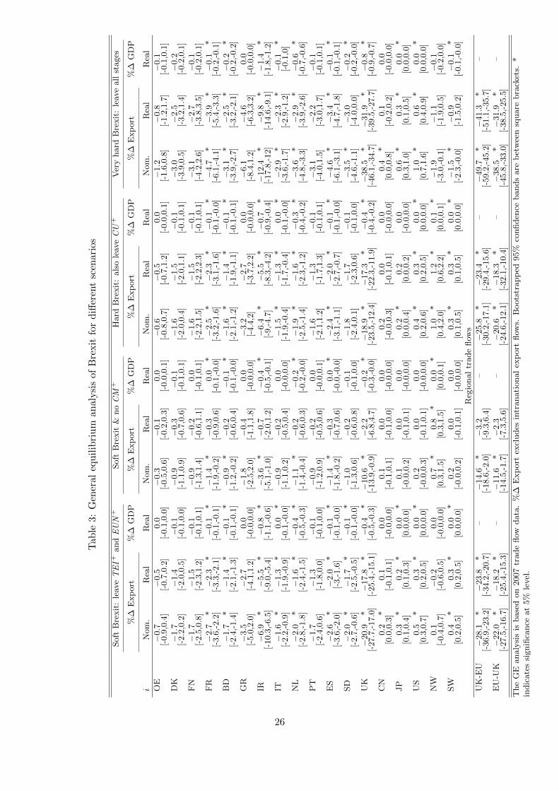
In Table 3 I display the result of four different Brexit scenarios ranging from soft to
very hard Brexit. In each scenario the UK leaves on additional stage. For each scenario I
will look at the country specific percentage change of nominal and real export, excluding
intranational export flows, and of real gdp, where the latter is derived using (A.20).
Finally, I also report the percentage change of nominal and real export for exports of
the UK to the EU and vice versa.
25
Tab
le3:
Gen
eral
equ
ilib
riu
man
alysi
sof
Bre
xit
for
diff
eren
tsc
enar
ios
Soft
Bre
xit
:le
aveTEI+
andEUN
+Soft
Bre
xit
&noCM
+H
ard
Bre
xit
:als
ole
aveCU
+V
ery
hard
Bre
xit
:le
ave
all
stages
%∆
Exp
ort
%∆
GD
P%
∆E
xp
ort
%∆
GD
P%
∆E
xp
ort
%∆
GD
P%
∆E
xp
ort
%∆
GD
P
iN
om
.R
eal
Rea
lN
om
.R
eal
Rea
lN
om
.R
eal
Rea
lN
om
.R
eal
Rea
l
OE
−0.7
−0.5
0.0
−0.3
−0.1
0.0
−0.6
−0.5
0.0
−1.2
−0.8
−0.1
[-0.9
,0.4
][-
0.7
,0.2
][-
0.1
,0.0
][-
0.5
,0.6
][-
0.2
,0.3
][-
0.0
,0.1
][-
0.8
,0.7
][-
0.7
,1.2
][-
0.0
,0.1
][-
1.6
,0.8
][-
1.2
,1.7
][-
0.1
,0.1
]D
K−
1.7
−1.4
−0.1
−0.9
−0.3
−0.1
−1.6
−1.5
−0.1
−3.0
−2.5
−0.2
[-2.2
,0.2
][-
2.0
,0.5
][-
0.1
,0.0
][-
1.1
,0.9
][-
0.7
,0.6
][-
0.1
,0.1
][-
2.0
,0.4
][-
2.0
,1.1
][-
0.1
,0.1
][-
3.9
,0.5
][-
3.2
,1.4
][-
0.2
,0.1
]F
N−
1.7
−1.5
−0.1
−0.9
−0.2
0.0
−1.6
−1.5
−0.1
−3.1
−2.7
−0.1
[-2.5
,0.8
][-
2.3
,1.2
][-
0.1
,0.1
][-
1.3
,1.4
][-
0.6
,1.1
][-
0.1
,0.1
][-
2.2
,1.5
][-
2.2
,2.3
][-
0.1
,0.1
][-
4.2
,2.6
][-
3.8
,3.5
][-
0.2
,0.1
]F
R−
2.7
*−
2.3
*−
0.1
*−
1.4
*−
0.3
0.0
*−
2.5
*−
2.3
*−
0.1
*−
4.7
*−
3.9
*−
0.1
*[-
3.6
,-2.2
][-
3.3
,-2.1
][-
0.1
,-0.1
][-
1.9
,-0.2
][-
0.9
,0.6
][-
0.1
,-0.0
][-
3.2
,-1.6
][-
3.1
,-1.6
][-
0.1
,-0.0
][-
6.1
,-4.1
][-
5.4
,-3.3
][-
0.2
,-0.1
]B
D−
1.7
*−
1.4
*−
0.1
*−
0.9
*−
0.2
−0.1
*−
1.6
*−
1.4
*−
0.1
*−
3.1
*−
2.5
*−
0.2
*[-
2.4
,-1.4
][-
2.1
,-1.3
][-
0.1
,-0.1
][-
1.2
,-0.2
][-
0.6
,0.4
][-
0.1
,-0.0
][-
2.1
,-1.2
][-
1.9
,-1.1
][-
0.1
,-0.1
][-
3.9
,-2.7
][-
3.2
,-2.1
][-
0.2
,-0.2
]G
R−
3.5
−2.7
0.0
−1.8
−0.4
0.0
−3.2
−2.7
0.0
−6.1
−4.6
0.0
[-5.0
,2.0
][-
4.1
,1.2
][-
0.0
,0.0
][-
2.5
,2.0
][-
1.1
,1.8
][-
0.0
,0.0
][-
4.4
,2]
[-3.7
,2.2
][-
0.0
,0.0
][-
8.4
,1.2
][-
6.3
,3.2
][-
0.0
,0.0
]IR
−6.9
*−
5.5
*−
0.8
*−
3.6
*−
0.7
−0.4
*−
6.4
*−
5.5
*−
0.7
*−
12.4
*−
9.8
*−
1.4
*[-
10.3
,-6.5
][-
9.0
,-5.4
][-
1.1
,-0.6
][-
5.1
,-1.0
][-
2.0
,1.2
][-
0.5
,-0.1
][-
9,-
4.7
][-
8.3
,-4.2
][-
0.9
,-0.4
][-
17.8
,-12]
[-14.6
,-9.1
][-
1.8
,-1.2
]IT
−1.6
*−
1.3
*0.0
*−
0.9
−0.2
0.0
−1.5
*−
1.3
*0.0
*−
2.9
*−
2.3
*−
0.1
*[-
2.2
,-0.9
][-
1.9
,-0.9
][-
0.1
,-0.0
][-
1.1
,0.2
][-
0.5
,0.4
][-
0.0
,0.0
][-
1.9
,-0.4
][-
1.7
,-0.4
][-
0.1
,-0.0
][-
3.6
,-1.7
][-
2.9
,-1.2
][-
0.1
,0]
NL
−2.0
*−
1.6
*−
0.4
*−
1.1
*−
0.2
−0.2
*−
1.9
*−
1.6
*−
0.3
*−
3.6
*−
2.9
*−
0.6
*[-
2.8
,-1.8
][-
2.4
,-1.5
][-
0.5
,-0.3
][-
1.4
,-0.4
][-
0.6
,0.3
][-
0.2
,-0.0
][-
2.5
,-1.4
][-
2.3
,-1.2
][-
0.4
,-0.2
][-
4.8
,-3.3
][-
3.9
,-2.6
][-
0.7
,-0.6
]P
T−
1.7
−1.3
−0.1
−0.9
−0.2
0.0
−1.6
−1.3
−0.1
−3.1
−2.2
−0.1
[-2.4
,0.6
][-
1.8
,0.0
][-
0.1
,0.0
][-
1.2
,0.9
][-
0.5
,0.6
][-
0.0
,0.1
][-
2.1
,1.2
][-
1.7
,1.3
][-
0.1
,0.1
][-
4.0
,1.5
][-
3.0
,1.7
][-
0.1
,0.1
]E
S−
2.6
*−
2.0
*−
0.1
*−
1.4
*−
0.3
0.0
*−
2.4
*−
2.0
*−
0.1
*−
4.6
*−
3.4
*−
0.1
*[-
3.6
,-2.0
][-
3,-
1.6
][-
0.1
,-0.0
][-
1.8
,-0.2
][-
0.7
,0.6
][-
0.0
,-0.0
][-
3.1
,-1.1
][-
2.7
,-0.7
][-
0.1
,-0.0
][-
6.1
,-3.1
][-
4.7
,-1.8
][-
0.1
,-0.1
]SD
−2.0
*−
1.7
*−
0.1
*−
1.0
−0.2
−0.1
−1.8
−1.7
−0.1
−3.5
*−
3.0
−0.2
*[-
2.7
,-0.6
][-
2.5
,-0.5
][-
0.1
,-0.0
][-
1.3
,0.6
][-
0.6
,0.8
][-
0.1
,0.0
][-
2.4
,0.1
][-
2.3
,0.6
][-
0.1
,0.0
][-
4.6
,-1.1
][-
4.0
,0.0
][-
0.2
,-0.0
]U
K−
20.9
*−
17.8
*−
0.4
*−
10.6
*−
2.2
−0.2
*−
18.9
*−
17.3
*−
0.4
*−
38.5
*−
31.9
*−
0.8
*[-
27.7
,-17.0
][-
25.4
,-15.1
][-
0.5
,-0.3
][-
13.9
,-0.9
][-
6.8
,4.7
][-
0.3
,-0.0
][-
23.5
,-12.4
][-
22.3
,-11.9
][-
0.4
,-0.2
][-
46.1
,-34.7
][-
39.5
,-27.7
][-
0.9
,-0.7
]C
N0.2
*0.1
0.0
0.1
0.0
0.0
0.2
0.0
0.0
0.4
*0.1
0.0
[0.0
,0.3
][-
0.1
,0.1
][-
0.0
,0.0
][-
0.1
,0.1
][-
0.1
,0.0
][-
0.0
,0.0
][-
0.0
,0.3
][-
0.1
,0.1
][-
0.0
,0.0
][0
.0,0
.8]
[-0.2
,0.2
][-
0.0
,0.0
]JP
0.3
*0.2
*0.0
*0.1
0.0
0.0
0.2
*0.2
0.0
0.6
*0.3
*0.0
*[0
.1,0
.4]
[0.1
,0.3
][0
.0,0
.0]
[-0.0
,0.2
][-
0.1
,0.1
][-
0.0
,0.0
][0
.0,0
.4]
[0.0
,0.2
][-
0.0
,0.0
][0
.3,1
.0]
[0.1
,0.5
][0
.0,0
.0]
US
0.5
*0.3
*0.0
*0.2
0.0
0.0
0.4
*0.3
*0.0
*1.0
*0.6
*0.0
*[0
.3,0
.7]
[0.2
,0.5
][0
.0,0
.0]
[-0.0
,0.3
][-
0.1
,0.1
][-
0.0
,0.0
][0
.2,0
.6]
[0.2
,0.5
][0
.0,0
.0]
[0.7
,1.6
][0
.4,0
.9]
[0.0
,0.0
]N
W0.1
−0.2
0.0
0.7
*0.8
*0.0
*1.0
*1.2
*0.1
*−
1.9
−1.1
−0.1
[-0.4
,0.7
][-
0.6
,0.5
][-
0.0
,0.0
][0
.3,1
.5]
[0.3
,1.5
][0
.0,0
.1]
[0.4
,2.0
][0
.6,2
.2]
[0.0
,0.1
][-
3.0
,-0.1
][-
1.9
,0.5
][-
0.2
,0.0
]SW
0.4
*0.3
*0.0
*0.2
0.0
0.0
0.3
*0.3
*0.0
*−
1.5
*−
0.9
−0.1
*[0
.2,0
.5]
[0.2
,0.5
][0
.0,0
.0]
[-0.0
,0.2
][-
0.1
,0.1
][-
0.0
,0.0
][0
.1,0
.5]
[0.1
,0.5
][0
.0,0
.0]
[-2.3
,-0.0
][-
1.5
,0.2
][-
0.1
,-0.0
]R
egio
nal
trade
flow
s
UK
-EU
−28.1
*−
23.8
*–
−14.6
*−
3.2
–−
25.8
*−
23.4
*–
−49.7
*−
41.3
*–
[-36.9
,-23.2
][-
34.2
,-20.7
][-
18.6
,-2.0
][-
9.3
,6.4
][-
30.2
,-17.1
][-
29.4
,-15.6
][-
59.2
,-45.2
][-
51.1
,-35.7
]E
U-U
K−
22.0
*−
18.2
*–
−11.6
*−
2.3
–−
20.6
*−
18.3
*–
−38.5
*−
31.9
*–
[-27.5
,-16.7
][-
25.4
,-15.3
][-
14.5
,-1.7
][-
7.3
,5.6
][-
24.6
,-12.1
][-
32.1
,-10.4
][-
45.8
,-33.0
][-
38.5
,-25.5
]
The
GE
analy
sis
isbase
don
2007
trade
flow
data
.%
∆E
xp
ort
excl
udes
intr
anati
onal
exp
ort
flow
s.B
oots
trapp
ed95%
confiden
cebands
are
bet
wee
nsq
uare
bra
cket
s.*
indic
ate
ssi
gnifi
cance
at
5%
level
.
26

In the first scenario, soft Brexit, the UK leaves Balassa stages 5 and 4, TEI +
and EUN +, respectively. These two stages encompass supranational bodies to arrange
cooperation on fiscal and monetary policy and standardization of national laws to
improve economic policy cooperation, respectively. It is most likely that this is going
to be the minimal outcome of Brexit. Both the EU countries and the UK lose in terms
of real exports, but not all loses are significant. The economic mechanism behind
this is that an increase in the bilateral trade barrier bijt leads to higher costs for the
UK to import from the EU reducing export and vice versa (see also Section 3.1).
The significant loses are somewhere between 2.3% and 1.4% except for Ireland that
loses more than double compared to the worst of all other EU countries. This can
be explained by the close Anglo-saxon ties between Ireland and the UK. However, no
EU country loses so much as the UK itself with 17.8%. But it is Ireland that suffers
the most in terms of real GDP, double that of the UK itself. The Netherlands is an
other country that is hit particularly hard with its small open economy. The UK loses
more than the EU in terms of the total export between the UK and the EU. The fall
in export from the UK to the EU is actually more than the overall fall implying that
the UK partially compensates the loss by exporting more to other non-EU countries,
i.e. trade diversion, mitigating the cost of Brexit. Because the exporter MR of the
UK rises, due to a higher bilateral trade barrier with the EU, there is less demand
for its goods leading to a drop in the price, so the UK becomes cheaper for non-EU
countries leading to more exports to non-EU countries. All non-EU countries gain,
from the Brexit, although the gains are small and not always significant. This is a
typical example of trade diversion (see Section 2.1).
The second scenario is a soft Brexit, where the UK additionally leaves Balassa stage
3, CM +; so leaving the SEA and restricting free movement of labour. Oddly enough
this scenario leads to lower real exports lose than the first scenario. This is because
CM + has a negative coefficient, see Table 2, due to the proximity versus concentration
trade-off. This does not necessarily imply that the second scenario is better than the
first scenario. One also has to analyze the effects of a decrease in labor and capital
mobility on real GDP through other channels like FDI and productivity. None of the
real export loses are significant, accept for Norway which gains due to trade diversion.
UK loses the most in terms of nominal exports, again followed by Ireland. The UK
is able to mitigate parts of the Brexit cost by trade creation with non-EU countries.
Ireland loses the most and twice as much as the UK in terms of real GDP.
The third scenario is a hard Brexit, where the UK leaves also Balassa stage 2, CU +.
In terms of size the effects are relatively comparable to a soft Brexit, the first scenario.
27

The UK loses by far the most from Brexit. The EU loses less from Brexit, but especially
Ireland is hit hard. The US, Norway and Switzerland gain from Brexit through trade
diversion.
Finally, the fourth scenario, the very hard Brexit, explores the consequences when
the negotiations completely fail and the UK stops all economic cooperation with the
EU leaving all five Balassa stages. This is by far the most harmful scenario for both the
UK and the EU. The UK’s real export is reduced by 31.9% leading to a 0.8% decrease
in real GDP, but similar to the other three scenarios the UK mitigates the cost of Brexit
partly by trade diversion to other non-EU countries. Also Ireland loses substantially
with 9.8% leading to a 1.4% decrease in real GDP. Ireland again loses by far the most in
terms of real GDP. Overall the pattern is similar to the other three scenarios. Note that
Switzerland and Norway, where it is only significant for the former, actually lose from
the very hard Brexit because the loss in exports due to the loss of an FTA with the UK
outweighs the export gains from trade diversion. All other non-EU countries gain from
a very hard Brexit thanks to trade diversion. This last scenario shows the importance
for the UK and the EU to agree upon an transition agreement for the years between
March 2019 and the day that they reach a final agreement. Because hammering out a
Brexit agreement takes likely more than two years after which automatically all treaties
between the EU and the UK are cancelled, as is specified by article 50.
As a final note I want to stress that these numbers, as presented above, should
not be considered as the final number for the cost of different Brexit scenarios. As I
mentioned before in this simple GE analysis I only look at the effects on exports and
completely ignore the effects on the financial sector, FDI, productivity et cetera. These
will most likely increase the impact of Brexit.
6.2 TTIP and CETA
In Table 4 I display the results of an FTA between the US and the EU (TTIP) and
between Canada and the EU (CETA). I assume that both FTAs are complete, i.e. FTA
gets full points. The setup of the table is similar as that of Table 3.
The US gains from TTIP are substantial with a 11.1% increase in real exports and
0.1% increase in real GDP. The gains in real exports for the US with only the EU are
even bigger, but the overall effect is smaller due to trade diversion. The UK and Ireland
gain the most from all the EU countries, most likely due to their close Anglo-saxon
ties with the US, where Ireland has the biggest increase in real GDP. All significant
gains of the EU countries are between 1.6%−2.1% increase in exports and 0.4%−0.1%
increase in real GDP. Non-EU countries experience a decrease in real exports due to
28
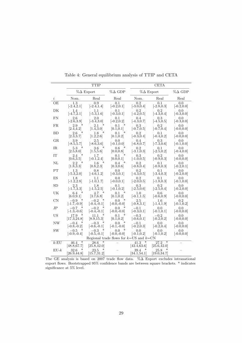
Table 4: General equilibrium analysis of TTIP and CETA
TTIP CETA
%∆ Export %∆ GDP %∆ Export %∆ GDP
i Nom. Real Real Nom. Real Real
OE 1.3 0.9 0.1 0.2 0.1 0.0[-2.4,2.1] [-2.4,1.4] [-0.2,0.1] [-3.0,0.4] [-2.8,0.3] [-0.2,0.0]
DK 1.4 1.1 0.1 0.2 0.2 0.0[-4.7,2.1] [-5.3,1.6] [-0.3,0.1] [-4.2,0.5] [-4.3,0.4] [-0.3,0.0]
FN 2.6 2.0 0.1 0.4 0.3 0.0[-2.6,3.9] [-3.4,3.0] [-0.2,0.2] [-4.3,0.7] [-4.5,0.5] [-0.3,0.0]
FR 2.9 * 2.1 * 0.1 * 0.3 0.2 0.0[2.4,4.2] [1.4,3.0] [0.1,0.1] [-0.7,0.5] [-0.7,0.4] [-0.0,0.0]
BD 2.6 * 1.8 * 0.1 * 0.2 0.1 0.0[2.3,3.7] [1.2,2.6] [0.1,0.2] [-0.3,0.4] [-0.4,0.2] [-0.0,0.0]
GR 3.9 2.5 0.0 0.4 0.3 0.0[-8.5,5.7] [-8.6,3.6] [-0.1,0.0] [-6.8,0.7] [-7.3,0.6] [-0.1,0.0]
IR 5.3 * 3.6 * 0.6 * 0.2 0.1 0.0[2.5,8.0] [1.5,5.6] [0.0,0.8] [-3.1,0.3] [-2.5,0.2] [-0.4,0.0]
IT 2.4 * 1.7 0.1 * 0.3 0.2 0.0[0.6,3.5] [-0.1,2.4] [0.0,0.1] [-1.0,0.5] [-0.9,0.3] [-0.0,0.0]
NL 2.2 * 1.6 * 0.4 * 0.2 0.1 0.0[1.8,3.3] [0.8,2.3] [0.3,0.6] [-0.8,0.4] [-0.8,0.3] [-0.2,0.1]
PT 1.3 0.8 0.0 0.2 0.1 0.0[-5.3,2.0] [-4.6,1.2] [-0.3,0.1] [-4.3,0.5] [-3.4,0.3] [-0.2,0.0]
ES 1.8 1.1 0.0 0.2 0.1 0.0[-1.2,2.8] [-1.0,1.7] [-0.0,0.1] [-2.0,0.5] [-1.8,0.3] [-0.1,0.0]
SD 2.3 1.8 0.1 0.3 0.2 0.0[-1.7,3.3] [-1.5,2.5] [-0.1,0.2] [-2.5,0.6] [-2.5,0.4] [-0.2,0.0]
UK 6.4 * 4.7 * 0.1 * 1.0 0.6 0.0[6.0,9.1] [3.7,6.8] [0.1,0.2] [-0.1,1.5] [-0.6,0.9] [-0.0,0.0]
CN −0.9 * −0.2 * 0.0 * 2.5 1.6 0.2[-1.7,-0.9] [-0.4,-0.1] [-0.0,-0.0] [-0.8,3.1] [-1.4,1.9] [-0.1,0.2]
JP −0.7 * −0.2 * 0.0 * −0.1 0.0 0.0[-1.3,-0.6] [-0.4,-0.1] [-0.0,-0.0] [-0.3,0.1] [-0.1,0.1] [-0.0,0.0]
US 17.9 * 11.1 * 0.1 * −0.3 −0.2 0.0[17.3,24.8] [8.9,15.3] [0.1,0.2] [-0.6,0.1] [-0.2,0.2] [-0.0,0.0]
NW −0.4 * −0.3 * 0.0 * −0.1 0.0 0.0[-0.8,-0.2] [-0.6,-0.1] [-0.1,-0.0] [-0.2,0.3] [-0.2,0.4] [-0.0,0.0]
SW −0.5 * −0.3 * 0.0 * 0.0 0.0 0.0[-0.9,-0.4] [-0.5,-0.1] [-0.0,-0.0] [-0.1,0.2] [-0.1,0.2] [-0.0,0.0]
Regional trade flows for k=US and k=CN
k-EU 46.4 * 28.6 * – 41.3 * 27.2 * –[48.8,67.7] [25.8,42.0] [42.4,63.6] [25.6,42.0]
EU-k 32.6 * 23.5 * – 39.4 * 25.8 * –[26.9,44.8] [15.7,31.2] [34.1,54.1] [19.0,34.7]
The GE analysis is based on 2007 trade flow data. %∆ Export excludes intranationalexport flows. Bootstrapped 95% confidence bands are between square brackets. * indicatessignificance at 5% level.
29

trade diversion. Surprisingly it is Norway and Switzerland that are hit hardest. One
would expect that Canada would suffer the most, being very close to the US, but it
actually suffers the least from all four non-EU countries.
The gains of CETA for Canada are small compared to the gains of TTIP for the
US and moreover they are insignificant. The same holds for all the EU countries and
non-EU countries. Still, the UK, of all EU countries, gains the most from CETA. Unlike
with TTIP, Ireland does not gain that much from CETA, it has actually one of the
smallest gains. The trade diversion effects for the non-EU countries are small. The US
is hit the hardest, most likely because it exports similar products as the EU to Canada.
This is supported by the two-digit Standard International Trade Classifications (SITC),
revision 3, of the UN Commodity Trade Statistics Database (UN Comtrade), which
shows that out of the ten most exported categories by the US to Canada and the EU
to Canada seven overlap. Hence, lower trade barriers between Canada and the EU
leads probably to trade diversion away from the US towards the EU. It is not clear why
CETA leads such smaller gains than TTIP. Further research must shed more light on
this result.
7 Robustness analysis
In this section I will perform two robustness checks. First, I relax the homogeneous
parameter assumption and allow for exporter and importer specific parameters. Second,
I investigate the effect of omitting τij · t on the GABI index estimates.
7.1 Parameter heterogeneity
In column 1 and 2 of Table 5 I investigate relaxing the homogeneous parameter as-
sumption. I allow for an overall parameter and both exporter- and importer-specific
parameters for the GABI index variables, for example
GABI ′ijtβ +∑i
GABI ′ijtβxi +
∑j
GABI ′ijtβmj , (9)
where I normalize the mean of both the exporter- and importer-specific parameters to
zero to prevent multicollinearity with the overall GABI variable. So, I untangle the
effects of the former two from the overall effect and the overall plus the exporter- or
importer-specific effect is the total exporter- or importer-specific effect, respectively.
For brevity I only report the overall effect in Table 5, but in Table C.2 I also report all
heterogeneous parameters. I do not consider country-pair specific parameters because
30
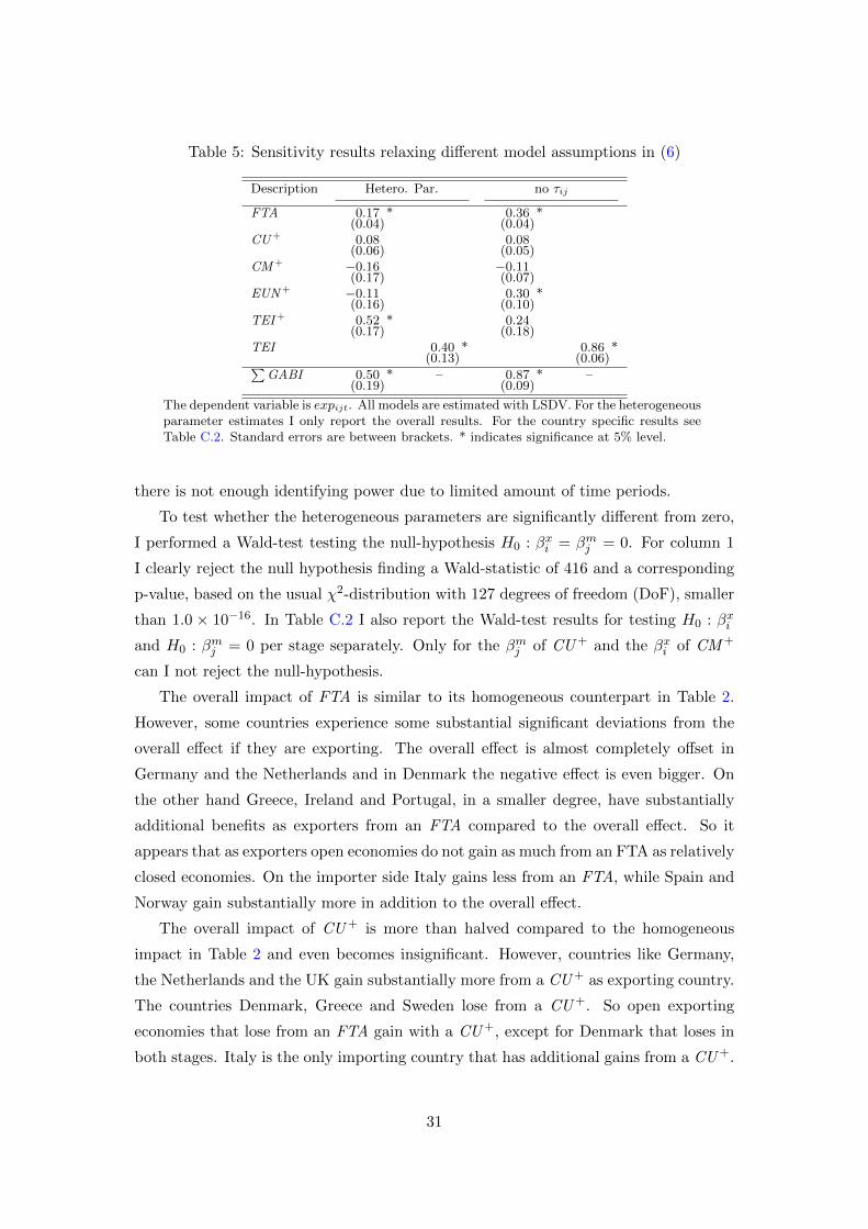
Table 5: Sensitivity results relaxing different model assumptions in (6)
Description Hetero. Par. no τij
FTA 0.17 * 0.36 *(0.04) (0.04)
CU+ 0.08 0.08(0.06) (0.05)
CM+ −0.16 −0.11(0.17) (0.07)
EUN+ −0.11 0.30 *(0.16) (0.10)
TEI+ 0.52 * 0.24(0.17) (0.18)
TEI 0.40 * 0.86 *(0.13) (0.06)∑
GABI 0.50 * – 0.87 * –(0.19) (0.09)
The dependent variable is expijt. All models are estimated with LSDV. For the heterogeneousparameter estimates I only report the overall results. For the country specific results seeTable C.2. Standard errors are between brackets. * indicates significance at 5% level.
there is not enough identifying power due to limited amount of time periods.
To test whether the heterogeneous parameters are significantly different from zero,
I performed a Wald-test testing the null-hypothesis H0 : βxi = βmj = 0. For column 1
I clearly reject the null hypothesis finding a Wald-statistic of 416 and a corresponding
p-value, based on the usual χ2-distribution with 127 degrees of freedom (DoF), smaller
than 1.0 × 10⁻¹⁶. In Table C.2 I also report the Wald-test results for testing H0 : βxi
and H0 : βmj = 0 per stage separately. Only for the βmj of CU + and the βxi of CM +
can I not reject the null-hypothesis.
The overall impact of FTA is similar to its homogeneous counterpart in Table 2.
However, some countries experience some substantial significant deviations from the
overall effect if they are exporting. The overall effect is almost completely offset in
Germany and the Netherlands and in Denmark the negative effect is even bigger. On
the other hand Greece, Ireland and Portugal, in a smaller degree, have substantially
additional benefits as exporters from an FTA compared to the overall effect. So it
appears that as exporters open economies do not gain as much from an FTA as relatively
closed economies. On the importer side Italy gains less from an FTA, while Spain and
Norway gain substantially more in addition to the overall effect.
The overall impact of CU + is more than halved compared to the homogeneous
impact in Table 2 and even becomes insignificant. However, countries like Germany,
the Netherlands and the UK gain substantially more from a CU + as exporting country.
The countries Denmark, Greece and Sweden lose from a CU +. So open exporting
economies that lose from an FTA gain with a CU +, except for Denmark that loses in
both stages. Italy is the only importing country that has additional gains from a CU +.
31

There are no importing countries that lose from a CU +.
The overall impact of CM + is almost halved compared to Table 2 and becomes
insignificant, although it is still negative. The Netherlands and Portugal have as ex-
porting countries an additional significant negative impact. That the Netherlands loses
so much from a CM + can be explained with proximity versus concentration trade off
and the fact that it has one of the biggest net inflows of FDI in percentage of GDP.
There is no exporting country that has an additional significant positive contribution.
As importer, Greece has an additional significant negative estimated impact and the
UK a positive estimated impact.
The overall impact of EUN + is insignificant like in Table 2. However, Finland,
Spain and the UK gain as exporter substantially from an EUN +. Italy and Spain have
additional gains importers from the EUN +. There is no significant negative exporter-
or importer-specific effect. So one can tentatively conclude that, if EUN + has any
significant overall effect, it is a positive effect.
Finally, the overall effect of the fifth Balassa stage TEI + is substantially larger than
in Table 2. For the exporting countries Denmark, Greece and Sweden have significant
substantial additional gains. On the other hand Ireland, Spain and the UK lose sub-
stantially. For the importing countries only Italy and Spain lose. Overall the estimated
exporter- and importer-specific effects of TEI + are the most dispersed of all Balassa
stages.
Summing all five overall Balassa stages, I find a larger estimate than what I find in
Table 2, but its standard error is also much bigger making this result hard to asses.
Finally, in column 2 of Table 5 I allow for heterogeneity in the estimated impact
of TEI . The Wald test cannot reject the null-hypothesis H0 : βxi = βmj = 0 finding
a Wald-statistic of 89 and a corresponding p-value, based on the usual χ2-distribution
with 29 DoF, of 5.4 × 10⁻⁸. The overall impact is slightly smaller than in Table 2.
The exporting countries Denmark, France, the Netherlands and the UK all have a sig-
nificant additional estimated positive gain. So in general, open economies gain more
from economic integration than other countries. Although Germany did not have a sig-
nificant additional gain. There were no exporting countries that suffer from economic
integration. Portugal and Norway have significant additional gains as importing coun-
tries from economic integration. The importing countries Finland and Ireland actually
have a net lose from economic integration.
Overall relaxing the homogeneous parameter assumption leads to more or less com-
parable results with the results in Table 2. Still, I reject the null-hypothesis that
the heterogeneous parameters are not significantly different from zero. The reduced
32
power, due to the heterogeneous parameters, might explain why I find more insignif-
icant estimates. The most important insight from heterogeneous parameters is that
open economies in general seem to benefit more from economic integration than closed
economies, except for the FTA stage where it is the other way around. Further research
in this area is needed to confirm this observation.
7.2 No country-pair trend FE
Although the inclusion of country-pair trend FE τij ·t is already becoming more common
after the paper of Bun & Klaassen (2007) (cf. Baier et al. (2014) and Bergstrand et al.
(2015)), it is still not a standard future in empirical gravity models.
In Table 5 I show in column 3-4 what happens with the estimated impact of different
Balassa stages, if I do not include τij · t. I find a more than doubling in the FTA effect
compared to Table 2 estimates, while the estimated CU + and CM + effect both halve
and even become insignificant. At the same time the estimated EUN + effect increases
ten fold and becomes significant. This supports Bun & Klaassen (2007), who find that
the effect of the euro on exports becomes highly significant if one does not add country-
pair trend FE. Finally, the estimated TEI + effect stays almost the same but the effect
becomes insignificant. The sum of the estimated effects increases substantially and is
almost identical to the estimated aggregate TEI effect in column 4, the latter is almost
double that of the estimate in Table 2.
If I perform a Wald-test to test H0 : τij = 0, I clearly reject the null-hypothesis
finding a Wald-statistic of 7661 and a corresponding p-value, based on the usual χ2-
distribution with 289 DoF, smaller than 1.0 × 10⁻¹⁶. Hence, omitting τij · t leads to
substantially biased estimates.
8 Conclusion
In this paper I have constructed a new way to measure the bilateral and gradual aspects
of economic integration, the gradual and bilateral integration (GABI) index. It uses the
principle of the multilateral ECB index, that divides EIAs into smaller events, assigning
each with a weighting to one of the five Balassa stages of economic integration. The
higher the weighting the bigger the contribution to economic integration. The GABI
is constructed for the five Balassa stages as well as for the aggregate of economic
integration.
This new measure has four advantages. First, it allows for differences in both the
depth and path of economic integration for all five Balassa stages in contrast with the
33
binary dummy variable, that is commonly used in the literature to capture economic
integration. Second, it allows for the identification of the different Balassa stages of
economic integration, which is often not possible with dummy variables because they
overlap causing potential multicollinearity. Third, it allows for identification of the
dynamic impact of the Balassa stages because lags solely capture the dynamics instead
of partly capturing the gradual aspect of economic, as is the case with dummy variables.
Finally, opposite to the multilateral ECB index, its bilateral aspects allows me to use
it as dependent variable in a bilateral export model.
I use a gravity model framework to estimate the impact of the GABI index for
the five Balassa stages using different model specifications and estimation methods.
We find that accounting for the depth and path of economic integration improves the
estimation results and therefore the GABI index indeed allows for a better identification
of both the long-run and the dynamic impact of the five Balassa stages.
Next, I use the estimated impact of the different Balassa stages in a GE analysis
to evaluate four different Brexit scenarios, ranging from a soft Brexit to a very hard
Brexit. The latter scenario leads to a 32% decrease in real exports and a 0.8% decrease
in real GDP for the UK. Other EU members also lose from Brexit, especially Ireland
and small open economies like the Netherlands. Non-EU members actually gain from
Brexit due to trade diversion effects. Similarly, to Brexit I investigate the impact of
TTIP and CETA on both the particpating countries and non-participating countries.
TTIP has a substantial effect on both the US and the EU, while CETA has a much
smaller and insignificant effect.
In future research the GABI index can be extended including more countries and
economic integration agreements. Another improvement is to find a more objective
way to establish the weighting of different economic integration events.
34

References
Anderson, James E. 1979. A Theoretical Foundation for the Gravity Equation. Amer-
ican Economic Review, 69(1), pp. 106–116.
Anderson, James E., & van Wincoop, Eric. 2003. Gravity with Gravitas: A Solution
to the Border Puzzle. The American Economic Review, 93(1), pp. 170–192.
Anderson, James E., & van Wincoop, Eric. 2004. Trade Costs. Journal of Economic
Literature, 42(3), pp. 691–751.
Anderson, James E., Larch, Mario, & Yotov, Yoto V. 2015. Estimating General Equi-
librium Trade Policy Effects: GE PPML. Tech. rept.
Arvis, Jean-Francois, & Shepherd, Ben. 2013. The Poisson quasi-maximum likelihood
estimator: a solution to the ‘adding up’ problem in gravity models. Applied Eco-
nomics Letters, 20(6), pp. 515–519.
Baier, Scott L., & Bergstrand, Jeffrey H. 2007. Do free trade agreements actually
increase members’ international trade? Journal of International Economics, 71(1),
pp. 72–95.
Baier, Scott L., Bergstrand, Jeffrey H., & Feng, Michael. 2014. Economic integra-
tion agreements and the margins of international trade. Journal of International
Economics, 93(2), pp. 339–350.
Balassa, Bela A. 1961. The theory of economic integration. Irwin series in economics.
R.D. Irwin.
Bergstrand, Jeffrey H. 1985. The Gravity Equation in International Trade: Some
Microeconomic Foundations and Empirical Evidence. The Review of Economics and
Statistics, 67(3), pp. 474–481.
Bergstrand, Jeffrey H., Larch, Mario, & Yotov, Yoto V. 2015. Economic integration
agreements, border effects, and distance elasticities in the gravity equation. European
Economic Review, 78, pp. 307–327.
Brainard, S. Lael. 1997. An Empirical Assessment of the Proximity-Concentration
Trade-off Between Multinational Sales and Trade. The American Economic Review,
87(4), pp. 520–544.
35
Bun, Maurice J. G., & Klaassen, Franc J. G. M. 2007. The Euro Effect on Trade is
not as Large as Commonly Thought. Oxford Bulletin of Economics and Statistics,
69(4), pp. 473–496.
Cipollina, Maria, & Salvatici, Luca. 2010. Reciprocal Trade Agreements in Gravity
Models: A Meta-Analysis. Review of International Economics, 18(1), pp. 63–80.
Dorrucci, Ettore, Fratzscher, Marcel, Mongelli, Francesco P., & Firpo, Stefano. 2002
(Oct.). European Integration: what lessons for other regions? The case of Latin
America. Working Paper Series. European Central Bank.
Dorrucci, Ettore, Firpo, Stefano, Fratzscher, Marcel, & Mongelli, Francesco Paolo.
2005. The Path of European Institutional and Economic Integration: What Lessons
for Latin America? Journal of Economic Integration, 20(2), pp. 217–251.
Dorrucci, Ettore, Ioannou, Demosthenes, Mongelli, Francesco, & Terzi, Alessio. 2015.
The four unions ”PIE” on the Monetary Union ”CHERRY”: a new index of Euro-
pean Institutional Integration. Occasional Paper Series 160. European Central Bank.
Dur, Andreas, Baccini, Leonardo, & Elsig, Manfred. 2014. The design of international
trade agreements: Introducing a new dataset. The Review of International Organi-
zations, 9(3), pp. 353–375.
Egger, Peter. 2000. A note on the proper econometric specification of the gravity
equation. Economics Letters, 66(1), pp. 25–31.
Egger, Peter, & Larch, Mario. 2012. Estimating Consistent Border Effects in Gravity
Models with Multilateral Resistance. The World Economy, 35(9), pp. 1121–1125.
Egger, Peter, & Tarlea, Filip. 2017. Comparing Apples to Apples: Estimating Consis-
tent Partial Effects of Preferential Economic Integration Agreements. CEPR Discus-
sion Papers 11894. C.E.P.R. Discussion Papers.
Fally, Thibault. 2015. Structural gravity and fixed effects. Journal of International
Economics, 97(1), pp. 76–85.
Frankel, Jeffrey A. 1997. Regional Trading Blocs in the World Economic System. Pe-
terson Institute Press: All Books, no. 72. Peterson Institute for International Eco-
nomics.
Head, Keith, & Mayer, Thierry. 2014. Gravity Equations: Workhorse,Toolkit, and
Cookbook. Handbook of International Economics, vol. 4. Elsevier. Chap. 3, pages
pp. 131–195.
36

Heckscher, Eli. 1919. The Effects of Foreign Trade on the Distribution of Income.
Ekonomisk Tidskrift, 21, pp. 497–512.
Helpman, Elhanan, Melitz, Marc J., & Yeaple, Stephen R. 2004. Export Versus FDI
with Heterogeneous Firms. American Economic Review, 94(1), pp. 300–316.
Klaassen, Franc, & Teulings, Rutger. 2015a. Untangling Multilateral Boundaries. Work-
ing Paper. University of Amsterdam.
Klaassen, Franc J. G. M., & Teulings, Rutger. 2015b (December 24). Untangling Fixed
Effects and Constant Regressors. Tech. rept. 15-137/VI. Tinbergen Institute Discus-
sion Paper.
Melitz, Marc J. 2003. The Impact of Trade on Intra-Industry Reallocations and Ag-
gregate Industry Productivity. Econometrica, 71(6), pp. 1695–1725.
Newey, Whitney K., & West, Kenneth D. 1987. A Simple, Positive Semi-definite, Het-
eroskedasticity and Autocorrelation Consistent Covariance Matrix. Econometrica,
55(3), pp. 703–708.
Newey, Whitney K., & West, Kenneth D. 1994. Automatic Lag Selection in Covariance
Matrix Estimation. Review of Economic Studies, 61(4), pp. 631–653.
Ohlin, Bertil. 1933. Interregional and international trade. Harvard University Press.
Rivera-Batiz, Luis A., & Romer, Paul M. 1991. Economic Integration and Endogenous
Growth. The Quarterly Journal of Economics, 106(2), pp. 531–555.
Roy, Jayjit. 2010. Do Customs Union Members Engage in More Bilateral Trade than
Free-Trade Agreement Members? Review of International Economics, 18(4), pp.
663–681.
Santos-Silva, Joao M. C., & Tenreyro, Silvana. 2006. The Log of Gravity. The Review
of Economics and Statistics, 88(4), pp. 641–658.
Tinbergen, J. 1962. Shaping the World Economy; Suggestions for an International
Economic Policy. Twentieth Century Fund, New York.
Viner, Jacob. 1950. The customs union issue. Studies in the administration of inter-
national law and organization. Carnegie Endowment for International Peace.
37

A General equilibrium analysis in the nominal model
Start with the nominal gravity model15 satisfying the following conditions
Xjijt = wyit
(bijt/SijtΠitPjt
)1−σEjt, (A.1)
Πit =
∑j
(bijt/SijtPjt
)1−σwej
11−σ
, (A.2)
Pjt =
(∑i
(bijt/Sijt
Πit
)1−σwyi
) 11−σ
, (A.3)
Yit =∑j
Xijt = pitQit, (A.4)
pit =
(wyitλit
) 11−σ 1
Πit, (A.5)
Yit = φitEit, (A.6)
where pit is the equilibrium price, wyit = YitYWt
and wejt =EjtEWt
(realize that YWt = EWt),
Qit is the total output of good i by country i at time t (where Qit =∑
i xijt) and φit is
an exogenous parameter allowing for unbalanced trade of country i at time t. I assume
that λit, Sijt, YWt and Qit are exogenous and do not change if bijt changes. Realize
that Sijt = SiUStSUSjt.
Besides (A.1)-(A.3), which are already presented in Section 3.1, we have three
additional underlying equations. First, (A.4) is the market clearing condition. This
helps us to derive (A.5), the equilibrium price. Finally, (A.6) is the balanced trade
condition, where φit allows for imbalanced trade.
So, in total I have six unknown variables that change when the trade barrier changes:
Xjijt, Yit, Ejt, Πit, Pjt and pit. To solve for these six unknowns Anderson et al. (2015)
developed the following iteration procedure based on (A.1)-(A.6).
15This section is in addition to Section 3.1.
38
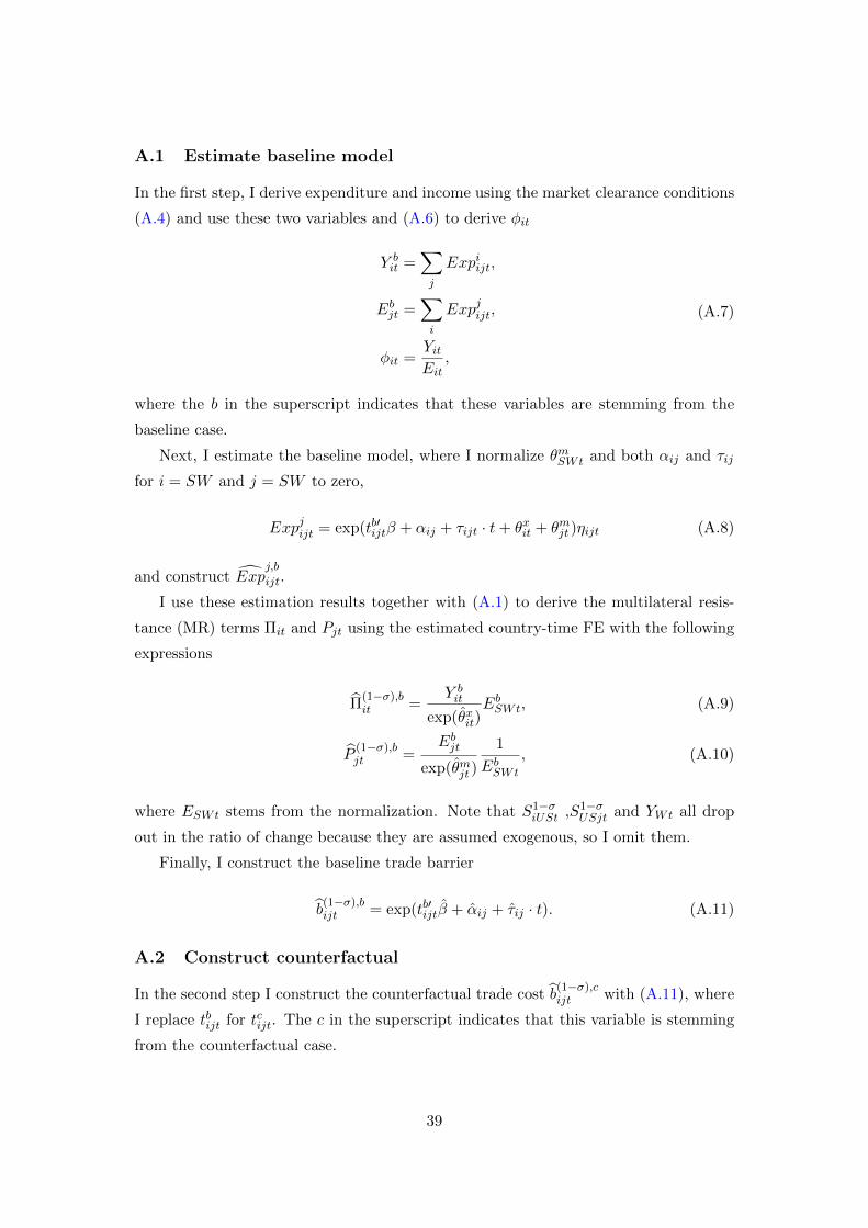
A.1 Estimate baseline model
In the first step, I derive expenditure and income using the market clearance conditions
(A.4) and use these two variables and (A.6) to derive φit
Y bit =
∑j
Expiijt,
Ebjt =∑i
Expjijt,
φit =YitEit
,
(A.7)
where the b in the superscript indicates that these variables are stemming from the
baseline case.
Next, I estimate the baseline model, where I normalize θmSWt and both αij and τij
for i = SW and j = SW to zero,
Expjijt = exp(tb′ijtβ + αij + τijt · t+ θxit + θmjt )ηijt (A.8)
and construct Expj,b
ijt.
I use these estimation results together with (A.1) to derive the multilateral resis-
tance (MR) terms Πit and Pjt using the estimated country-time FE with the following
expressions
Π(1−σ),bit =
Y bit
exp(θxit)EbSWt, (A.9)
P(1−σ),bjt =
Ebjt
exp(θmjt )
1
EbSWt
, (A.10)
where ESWt stems from the normalization. Note that S1−σiUSt ,S1−σ
USjt and YWt all drop
out in the ratio of change because they are assumed exogenous, so I omit them.
Finally, I construct the baseline trade barrier
b(1−σ),bijt = exp(tb′ijtβ + αij + τij · t). (A.11)
A.2 Construct counterfactual
In the second step I construct the counterfactual trade cost b(1−σ),cijt with (A.11), where
I replace tbijt for tcijt. The c in the superscript indicates that this variable is stemming
from the counterfactual case.
39

A.3 Estimate partial and conditional effect
In the third step I estimate the partial effect and the effect conditional on output and
expenditure being fixed.
A.3.1 Partial effect
The partial effect is estimate using (A.1)
Expp
ijt = Y bit
(bcijt
ΠbitP
bjt
)1−σ
Ebjt, (A.12)
where the p indicates that this estimate is stemming from the partial case. Note that
YWt and Sijt drop out when we calculate percentage change so we omit them here.
A.3.2 Conditional effect
Next I allow the multilateral resistance terms to change while keeping expenditure and
income fixed, the conditional effect.
I estimate the following model, while keeping b(1−σ),cijt fixed,
Expjijt = b(1−σ),cijt exp(θxit + θmjt )ηijt, (A.13)
and construct Expj,cnd
ijt , where cnd indicates that this estimate stems from the condi-
tional effect.
Next, I rederive the MR terms Π(1−σ),cndit and P
(1−σ),cndjt using the estimated country-
time FE and (A.9)-(A.10), respectively.
A.4 Estimate full endowment effect
In the fourth step I derive the full endowment case, allowing output and expenditure
to change as well, with an iteration procedure.
Therefore, I first need to construct the equilibrium price ratio as a starting value
for the iteration based on the expression for equilibrium prices (A.5):
pcndit
pbit=
(exp(θx,cndit )
exp(θx,bit )
EbSWt
EcndSWt
) 11−σ
,
pcndjt
pbjt=
(exp(θx,cndjt )
exp(θx,bjt )
EbSWt
EcndSWt
) 11−σ
.
(A.14)
40

Note that EcndSWt = EbSWt, so the expenditure ratio equals one. However, when I start
updating prices expenditure will start changing and therefore this ratio as well. Fur-
thermore, I will also use Expfull(1)
ijt = Expcnd
ijt , θx,full(2)it = θ
x,full(1)it = θx,cndit , θ
m,full(2)jt =
θm,full(1)jt = θm,cndjt and the ratios
(Πfull(1)it
Πfull(2)it
)1−σ=
(Πcndit
Πcndit
)1−σand
(Pfull(1)jt
Pfull(2)jt
)1−σ=(
P cndjt
P cndjt
)1−σas starting values. The full superscript indicates that these variables stem
from the full endowment GE analysis, where the numbers between bracket indicate the
iteration step.
A.4.1 Iterate to obtain full endowment effect
I start by updating the export variable with the following expression derived from (A.1)
Expj,full(2)
ijt =pfull(2)it
pfull(1)it
pfull(2)jt
pfull(1)jt
(Πfull(1)it
Πfull(2)it
Pfull(1)jt
Pfull(2)jt
)1−σ
Expj,full(1)
ijt , (A.15)
where I use that Yit = pitQit and, taking ratios, I getYfull(2)it
Yfull(1)it
=pfull(2)it
pfull(1)it
under the
assumption that Qit is exogenous.16 Note that Expj,full(2)
ijt has a tilde to distinguish it
from estimated export flows.
I use the newly generated export flows and the counterfactual trade cost to estimate
Expj,full(2)
ijt = b(1−σ),cijt exp(θ
x,full(3)it + θ
m,full(3)jt )εijt (A.16)
and construct Expj,full(2)
ijt .
Next, the predicted export flows can be used to derive income
Yfull(3)it =
∑j
Expj,full(2)
ijt . (A.17)
Consequently, expenditure Efull(3)jt follows from (A.6). I use the estimate exporter-time
16Note that Yit = pitQit seem to contradict each other Yit =∑j Xijt =
∑j bijtpitxijt, because the
latter shows that Yit depends on bijt as well. The intuition behind this is that there is a transportsector that contributes to the income of country i; this is different from the iceberg trade cost that isstandard in the literature. So to make these two definitions in line with each other we have to adjustthe former to Yit = pitQit
∑j bijt
xijtQit
. The problem of this expression is that it depends on real export.This leads to two problems. First, real export is hard to obtain in general because we need to agreeupon the appropriate deflator to deflate nominal export flows. Second, if we have agreed upon anappropriate deflator, say the exporter price index, we have to update the exporter price index withchanging equilibrium prices, complicating the GE analysis further. Solving this problem I leave forfuture research.
41

and importer-time FE and (A.14) to derive the new equilibrium price ratiospfull(3)it
pfull(2)it
andpfull(3)jt
pfull(2)jt
. Finally, I construct the new MR terms using the estimated θx,full(3)it and
θm,full(3)jt , output Y
full(3)it , expenditure E
full(3)jt and (A.9)-(A.10).
I iterate this process until the equilibrium price ratiopfull(3)it
pfull(2)it
does not change any-
more.
A.5 Derive full endowment GE effect
In the fifth and final step I derive the final equilibrium price ratiopfullit
pbitusing (A.14). I
use this ratio to generate income
Y fullit =
pfullit
pbitY bit (A.18)
and consequently expenditure Efulljt is constructed using (A.6). Next, the MR terms
are constructed using the estimated θx,fullit and θm,fulljt , output Y fullit , expenditure Efulljt
and (A.9)-(A.10).
Finally, I construct the new export flows based on (A.1)
Expj,full
ijt = Y fullit
(bcijt
Πfullit P fulljt
)1−σ
Efulljt . (A.19)
Now I can derive the percentage change in the full endowment GE with respect to
the baseline scenario as a consequence of a change in the counterfactual trade barrier.
Using the percentage change in the price ratiopfullit
pbitand the percentage change of P fulljt
I can also calculate the percentage change of full real GDP by
dyfullit
ybit= d
pfullit
pbit
−dP fulljt
P bjt, (A.20)
where dyfullit = yfullit − ybit and I use that yit = YitPit
implying that dyityit
= dYitYit
− dPitPit
,
where one has to realize that Yit = pitQit and Qit is exogenous.
42

B General equilibrium analysis in the real model
Start with the real gravity equation17 by Klaassen & Teulings (2015a) satisfying the
following equations
xijt =
(wyitλit
) −11−σ
wyit
(bijtsijtπit
)−σcjt, (B.1)
πit =
∑j
(bijtsijt
)1−σwejt
11−σ
, (B.2)
yit =∑j
xijt, (B.3)
pitPit
=
(wyitλit
) 11−σ 1
πit, (B.4)
cjt =1
φjt
pjtPjt
ψjtyjt, (B.5)
ψjt =∑i
bjitwxjit, (B.6)
where pitPit
is the relative equilibrium price,pjtPjtψjt is the terms of trade of country j
(an improvement increases the purchasing power of country j, while a deterioration
decreases the purchasing power of country j), wyit = yityWt
, wejt =cjtcWt
, wxjit =xjit∑i xjit
(realize that yWt = cWt) and φit is an exogenous parameter that allows for unbalanced
trade in country i at time t. I assume that yit, yjt, yWt, sijt, λit and λjt, are exogenous
and do not change if bijt changes.
Besides (B.1)-(B.2), which are already presented in Section 3.1, we have four addi-
tional underlying equations. First, (B.3) is the market clearing condition for quantity
of goods. This helps us to derive (B.4), the relative equilibrium price. Third, (B.5)
is the balanced trade condition, where φit allows for imbalanced trade. Finally, (B.6)
gives weighted bilateral trade cost.
So, in total I have five unknown variables that change when the trade barrier
changes: xijt,pitPit
, cjt, πit and ψjt. If I substitute (B.4) into (B.5) and the resulting
balanced trade expression into (B.1) and estimate the latter, I only have two unknowns
remaining: πit and ψjt. To solve for these final two unknowns I use a similar method
as in Section A. However, because I have only two unknowns that are fully captured
by the country-time FE, I no longer need to iterate; so there is no need to perform
step four from the nominal GE analysis, as described in Section A.4. Instead I can now
17This section is in addition to Section 3.1.
43
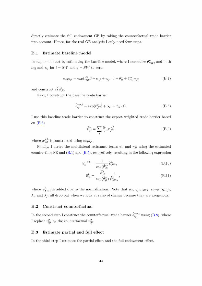
directly estimate the full endowment GE by taking the counterfactual trade barrier
into account. Hence, for the real GE analysis I only need four steps.
B.1 Estimate baseline model
In step one I start by estimating the baseline model, where I normalize θmSWt and both
αij and τij for i = SW and j = SW to zero,
expijt = exp(tb′ijtβ + αij + τijt · t+ θxit + θmjt )ηijt (B.7)
and construct expbijt.
Next, I construct the baseline trade barrier
b−σ,bijt = exp(tb′ijtβ + αij + τij · t). (B.8)
I use this baseline trade barrier to construct the export weighted trade barrier based
on (B.6)
ψbjt =∑i
bbjitwx,bjit , (B.9)
where wx,bjit is constructed using expijt.
Finally, I derive the multilateral resistance terms πit and πjt using the estimated
country-time FE and (B.1) and (B.5), respectively, resulting in the following expression
π−σ,bit =1
exp(θxit)ψbSWt, (B.10)
πbjt =ψbjt
exp(θmjt )
1
ψbSWt
, (B.11)
where ψbSWt is added due to the normalization. Note that yit, yjt, yWt, siUSt ,sUSjt,
λit and λjt all drop out when we look at ratio of change because they are exogenous.
B.2 Construct counterfactual
In the second step I construct the counterfactual trade barrier b−σ,cijt using (B.8), where
I replace tb′ijt by the counterfactual tc′ijt.
B.3 Estimate partial and full effect
In the third step I estimate the partial effect and the full endowment effect.
44

B.3.1 Partial effect
The partial effect is estimate by (B.1), resulting into
exppijt =
(bcijt
πbit
)−σψbjt
πbjt. (B.12)
Note that yit, yjt, yWt, sijt , λit and λjt drop out when we calculate percentage change
so we omit them here.
B.3.2 Full effect
Now I allow πit and πjt to change. I start by estimating the following model
expijt = b−σ,cijt exp(θxit + θmjt )ηijt (B.13)
and construct expfullijt . Note that b−σ,cijt is held fixed.
Next, I construct the weighted trade cost ψfulljt using the counterfactual trade barrier
bcjit and (B.9), where I use expfullijt to construct the export weights. Finally, I derive
the multilateral resistance terms πit and πit using the estimated country-time FE, ψfulljt
and (B.10)-(B.11).
B.4 Derive full endowment GE effect
In the fourth and final step I use the full endowment GE from Section B.3.2 to derive
the percentage change with respect to the baseline scenario from Section B.1 as a
consequence of the change in the counterfactual trade barrier.
C Additional tables
45

Table C.1: FTA starting dates and participating-countries for the FTA variable FTABBijt .
FTA name Start Participating countriesEuropean Union (EU) 1958 Austria (1995), Denmark (1973), Finland (1995), France,
Germany, Greece (1981), Ireland (1973), Italy, Netherlands,Portugal (1986), Spain (1986), Sweden (1995), United Kingdom (1973)
European Free Trade 1960 Austria (until 1995), Denmark (until 1973),Association (EFTA) Finland (1986-1995), Portugal (until 1986), Sweden (until 1995),
United Kingdom (Until 1973), Norway, SwitzerlandEU-EFTA 1973 Agreement between all EU and EFTA members
Finland enters in 1974 as associate EFTA memberCUSFTA 1989 United States and CanadaEuropean Economic Area (EEA) 1994 New agreement between all EU and EFTA membersNorth American Free 1994 United States, CanadaTrade Agreement (NAFTA)
Number between brackets are entry or exit dates of individual countries.
46
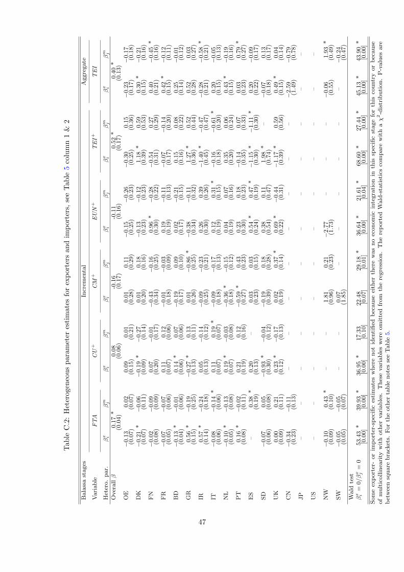
Tab
leC
.2:
Het
erog
eneo
us
par
amet
eres
tim
ates
for
exp
orte
rsan
dim
por
ters
,se
eT
able
5co
lum
n1
&2
Bala
ssa
stages
Incr
emen
tal
Aggre
gate
Vari
able
FTA
CU
+CM
+EUN
+TEI+
TEI
Het
ero.
par.
βx i
βm j
βx i
βm j
βx i
βm j
βx i
βm j
βx i
βm j
βx i
βm j
Over
allβ
0.1
7*
0.0
8-0
.16
-0.1
10.5
2*
0.4
0*
(0.0
4)
(0.0
6)
(0.1
7)
(0.1
6)
(0.1
7)
(0.1
3)
OE
−0.1
30.0
20.0
90.0
10.0
10.1
1−
0.1
5−
0.2
6−
0.3
00.1
5−
0.2
3−
0.1
7(0.0
7)
(0.0
7)
(0.1
5)
(0.2
1)
(0.2
8)
(0.2
9)
(0.2
5)
(0.2
3)
(0.2
5)
(0.3
6)
(0.1
7)
(0.1
8)
DK
−0.2
1*
−0.0
6−
0.1
9*
−0.2
70.0
10.1
8−
0.1
3−
0.1
21.1
8*
0.5
90.3
0*
−0.2
1(0.0
7)
(0.1
1)
(0.0
9)
(0.1
4)
(0.2
0)
(0.1
6)
(0.2
3)
(0.2
3)
(0.3
9)
(0.5
3)
(0.1
5)
(0.1
6)
FN
−0.0
2−
0.0
90.0
7−
0.0
1−
0.4
3−
0.1
60.9
6*
−0.2
8−
0.5
40.2
70.4
0−
0.4
5*
(0.0
8)
(0.0
9)
(0.2
0)
(0.1
7)
(0.3
4)
(0.2
5)
(0.3
0)
(0.2
2)
(0.3
1)
(0.2
9)
(0.2
1)
(0.1
6)
FR
−0.0
7−
0.0
70.1
10.1
2−
0.0
1−
0.0
30.1
9−
0.1
1−
0.0
7−
0.1
40.4
2*
−0.1
2(0.0
5)
(0.0
6)
(0.0
7)
(0.0
6)
(0.1
8)
(0.0
9)
(0.1
9)
(0.1
3)
(0.1
7)
(0.2
0)
(0.1
5)
(0.1
1)
BD
−0.1
3*
−0.0
10.1
4*
0.0
7−
0.1
90.0
90.0
2−
0.2
10.1
50.0
80.2
5−
0.0
1(0.0
4)
(0.0
6)
(0.0
6)
(0.0
6)
(0.1
7)
(0.1
0)
(0.1
7)
(0.1
5)
(0.1
6)
(0.2
2)
(0.1
4)
(0.1
2)
GR
0.5
6*
−0.1
9−
0.2
7*
0.1
30.0
1−
0.8
6*
−0.3
8−
0.1
11.2
7*
0.5
20.5
20.0
3(0.1
5)
(0.2
5)
(0.1
3)
(0.1
1)
(0.2
6)
(0.2
5)
(0.3
4)
(0.3
2)
(0.3
6)
(0.4
4)
(0.2
8)
(0.2
7)
IR0.5
7*
−0.2
40.0
5−
0.1
4−
0.0
9−
0.2
30.2
60.3
9−
1.4
0*
−0.4
7−
0.2
8−
0.5
8*
(0.1
4)
(0.1
8)
(0.1
3)
(0.1
2)
(0.2
5)
(0.2
1)
(0.3
0)
(0.2
6)
(0.4
5)
(0.4
7)
(0.2
1)
(0.2
1)
IT−
0.0
8−
0.1
4*
0.1
10.1
9*
−0.0
9−
0.1
70.1
20.3
1*
−0.1
6−
0.6
1*
0.2
0−
0.0
5(0.0
6)
(0.0
6)
(0.0
7)
(0.0
7)
(0.1
8)
(0.1
3)
(0.1
9)
(0.1
5)
(0.1
8)
(0.2
0)
(0.1
5)
(0.1
3)
NL
−0.1
0*
−0.1
30.1
9*
−0.0
3−
0.3
6*
−0.1
50.0
40.0
70.3
50.0
60.4
3*
−0.1
9(0.0
5)
(0.0
8)
(0.0
7)
(0.0
8)
(0.1
8)
(0.1
2)
(0.1
9)
(0.1
6)
(0.2
0)
(0.2
4)
(0.1
5)
(0.1
6)
PT
0.1
6*
−0.0
20.2
10.1
2−
0.5
9*
0.4
30.2
30.1
8−
0.1
40.0
70.0
30.7
9*
(0.0
8)
(0.1
1)
(0.1
9)
(0.1
6)
(0.2
7)
(0.2
3)
(0.3
0)
(0.2
3)
(0.3
5)
(0.3
3)
(0.2
3)
(0.2
7)
ES
–0.3
8*
0.2
0–
0.0
30.0
30.5
4*
0.4
7*
−1.1
5*
−1.1
1*
0.2
0−
0.0
9(0.1
9)
(0.1
3)
(0.2
3)
(0.1
5)
(0.2
4)
(0.1
9)
(0.3
0)
(0.3
0)
(0.2
2)
(0.1
7)
SD
−0.0
70.0
5−
0.9
3*
−0.0
4−
0.1
90.1
80.3
80.1
11.9
8*
–−
0.0
70.1
3(0.0
6)
(0.0
8)
(0.3
0)
(0.1
2)
(0.3
9)
(0.2
8)
(0.5
4)
(0.4
7)
(0.7
4)
(0.1
8)
(0.1
7)
UK
0.0
00.2
10.2
3*
−0.1
70.0
20.3
7*
0.6
9*
−0.4
4−
1.1
7*
0.5
90.4
9*
0.0
4(0.0
9)
(0.1
1)
(0.1
2)
(0.1
3)
(0.1
9)
(0.1
4)
(0.2
2)
(0.3
1)
(0.3
9)
(0.5
6)
(0.1
5)
(0.1
4)
CN
−0.3
4−
0.1
1–
––
––
––
–−
2.5
9−
0.7
9(0.2
3)
(0.1
3)
(1.4
9)
(0.7
8)
JP
––
––
––
––
––
––
US
––
––
––
––
––
––
NW
−0.1
00.4
3*
––
1.8
10.2
1−
2.7
7–
––
−0.0
61.9
3*
(0.0
9)
(0.1
0)
(0.9
6)
(0.2
3)
(1.7
3)
(0.5
5)
(0.4
9)
SW
−0.0
5−
0.0
5–
–0.0
7–
––
––
–−
0.2
4(0.0
5)
(0.0
7)
(1.8
5)
(0.4
7)
Wald
test
βx i
=0/βx j
=0
53.4
3*
39.9
3*
36.9
5*
17.3
322.4
829.1
8*
36.6
4*
21.6
1*
68.6
0*
27.4
4*
45.1
3*
43.9
0*
[0.0
0]
[0.0
0]
[0.0
0]
[0.1
0]
[0.0
7]
[0.0
1]
[0.0
0]
[0.0
4]
[0.0
0]
[0.0
0]
[0.0
0]
[0.0
0]
Som
eex
port
er-
or
imp
ort
er-s
pec
ific
esti
mate
sw
her
enot
iden
tified
bec
ause
eith
erth
ere
was
no
econom
icin
tegra
tion
inth
issp
ecifi
cst
age
for
this
countr
yor
bec
ause
of
mult
icollin
eari
tyw
ith
oth
erva
riable
s.T
hes
eva
riable
sw
ere
om
itte
dfr
om
the
regre
ssio
n.
The
rep
ort
edW
ald
-sta
tist
ics
com
pare
wit
haχ2-d
istr
ibuti
on.
P-v
alu
esare
bet
wee
nsq
uare
bra
cket
s.F
or
the
oth
erta
ble
note
sse
eT
able
5.
47