Discussion Papers

Brexit and Uncertainty in Financial Markets

Guglielmo Maria Caporale, Luis Gil-Alana and Tommaso Trani

1719

Deutsches Institut für Wirtschaftsforschung 2018

Opinions expressed in this paper are those of the author(s) and do not necessarily reflect views of the institute.

IMPRESSUM

© DIW Berlin, 2018

DIW Berlin German Institute for Economic Research Mohrenstr. 58 10117 Berlin

Tel. +49 (30) 897 89-0 Fax +49 (30) 897 89-200 http://www.diw.de

ISSN electronic edition 1619-4535

Papers can be downloaded free of charge from the DIW Berlin website: http://www.diw.de/discussionpapers

Discussion Papers of DIW Berlin are indexed in RePEc and SSRN: http://ideas.repec.org/s/diw/diwwpp.html http://www.ssrn.com/link/DIW-Berlin-German-Inst-Econ-Res.html

Brexit and Uncertainty in Financial Markets

Guglielmo Maria Caporale Brunel University London, CESifo and DIW Berlin

Luis Gil-Alana University of Navarra

Tommaso Trani University of Navarra

January 2018

Abstract

This paper applies long-memory techniques (both parametric and semi-parametric) to examine whether Brexit has led to any significant changes in the degree of persistence of the FTSE 100 Implied Volatility Index (IVI) and of the British pound’s implied volatilities (IVs) vis-à-vis the main currencies traded in the FOREX, namely the euro, the US dollar and the Japanese yen. We split the sample to compare the stochastic properties of the series under investigation before and after the Brexit referendum, and find an increase in the degree of persistence in all cases except for the British pound-yen IV, whose persistence has declined after Brexit. These findings highlight the importance of completing swiftly the negotiations with the EU to achieve an appropriate Brexit deal.

Keywords: Brexit, uncertainty, IVI index, British pound’s implied volatilities,

financial markets

JEL codes: C22, F30

Corresponding author: Professor Guglielmo Maria Caporale, Research Professor at DIW Berlin. Department of Economics and Finance, Brunel University, London, UB8 3PH, UK. Tel.: +44 (0)1895 266713. Fax: +44 (0)1895 269770. Email: Guglielmo-Maria.Caporale@brunel.ac.uk The second- and third-named authors gratefully acknowledge the financial support received from the Ministerio de Economía y Competitividad: ECO2014-55236 (Luis Alberiko Gil-Alana) and ECO2015-68815-P (Tommaso Trani) .

1

1. Introduction

The decision made by the UK to leave the EU as a result of the referendum held on 23

June 2016, commonly known as Brexit, undoubtedly represents a significant shock to

the UK economy. In particular, the resulting increase in uncertainty can be expected

to have a significant short-run impact on financial markets as well as sizeable long-

run effects on real economic activity owing to substantial structural changes to the

economy. The present study focuses on the former; more specifically, it applies long-

memory techniques (both parametric and semi-parametric) to examine whether Brexit

has led to any significant changes in the degree of persistence of the FTSE 100

Implied Volatility Index (IVI), which is a well-known measure of uncertainty in

European financial markets. To obtain further evidence we also examine the British

pound’s implied volatilities (IVs) vis-à-vis the main currencies traded in the foreign

exchange market (FOREX), namely the euro, the US dollar and the Japanese yen. In

all cases we split the sample and compare the stochastic properties of the series under

investigation before and after the Brexit referendum. To preview the results, we find

an increase in the degree of persistence of the IVI index as well as of the British

pound-US dollar IV and the euro-British pound IV, whilst there appears to have been

a decrease in the case of the British pound-yen IV.

Investor fear about the consequences of Brexit has already been reflected in

some asset prices. In particular, the perception of a higher sovereign default risk has

led to higher CDS spreads, and the greater uncertainty about future economic and

policy developments (see, e.g., Baker et al., 2016a) has been associated with wider

sovereign and corporate bond yield spreads as well as higher asset price volatility

(Kierzenkowski et al., 2016). Moreover, higher risk premia for the British pound have

2

led to an exchange rate depreciation, and a further fall of the British currency is

expected by most analysts.

The time series properties of expected risk indicators are clearly of great

interest. One of the most informative is the IVI index, which can be viewed as a

“fear” index. It is the European counterpart to the better known VIX index for the

Chicago stock market that most of the literature has examined. In particular, Whaley

(2000) suggests that the VIX can be interpreted as an ‘investor fear gauge’, that

reaches higher levels during periods of market turmoil. It is an implied volatility

index: the lower its level, the lower demand is from investors seeking to buy

protection against risk and thus the lower is the level of market fear. Most papers

analysing the VIX have focused on its predictive power for future returns (e.g., Giot,

2005; Guo and Whitelaw, 2006; Chow et al., 2014, 2016; Heydon et al., 2000).

Fleming et al. (1995) were the first to analyse the persistence of this index and found

that its daily changes follow an AR(1) process, whilst its weekly changes exhibit

mean reversion, and there is no evidence of seasonality. Long-memory behaviour in

the VIX was also detected by Koopman et al. (2005), Corsi (2009) and Fernandes et

al. (2014), as well as by Huskaj (2013) in its volatility. By contrast, Jo-Hui and Yu-

Fang (2014) found no evidence of long memory. Finally, Caporale et al. (2017) used

two different long-memory approaches (R/S analysis with the Hurst exponent method

and fractional integration) to assess the persistence of the VIX index over the period

2004-2016, as well as some sub-periods (pre-crisis, crisis and post-crisis). They found

that its properties change over time: in normal periods, the VIX exhibits anti-

persistence (there is a negative correlation between its past and future values), whilst

during crises its persistence increases.

3

In the present paper we analyse the effects of Brexit on the IVI index to assess

the extent to which the former has generated more persistent “fear” in financial

markets. Since the companies included in the FTSE 100 index make the majority of

their profits outside the UK, we extend our analysis to the British pound’s implied

volatilities (IVs) in order to obtain a more complete picture – in fact the suggestion

has been made by analysts that Brexit might have more pronounced and long-lasting

effects on the FOREX rather than on stock markets.

The layout of this paper is as follows. Section 2 describes the data, Section 3

outlines the methodology and discusses the empirical findings. Section 4 offers some

concluding remarks.

2. Data Description

Our sample consists of daily (end-of-the-day) observations on the following four time

series: the FTSE 100 Implied Volatility Index (IVI), the 3-month British pound-US

dollar IV, the 3-month euro-British pound IV, and the 3-month British pound-

Japanese yen IV.1 For the sake of brevity, henceforth we shall denote the latter three

series as GBP-USD IV, EUR-GBP IV and GBP-JPY IV respectively.

The FTSE 100 IVI is a series that measures the implied volatility of the

underlying FTSE 100 index. In particular, the IVI is an interpolation of 30, 60, 90,

180 and 360 day implied volatility estimates, which are based on the prices of out-of-

the-money options. As a result, the IVI provides an estimate of the market’s volatility

expectations on the underlying index between now and the index options’ expiration,

1 We focus on investors’ willingness to buy protection against fluctuations in the British pound over the following three months because this was the approach of various multinationals considering the likely effects of Brexit just before the date of the referendum (Kierzenkowski et al., 2016). Moreover, the volatility implied by 1-month currency options follows very similar patterns to the one implied by 3-month ones, the only difference being that the former display larger swings than the latter.

4

and therefore provides useful information to market participants for the purpose of

risk management. It is forward-looking, and can be seen as an indicator of market

sentiment/fear. Similarly, the British pound’s IV series are measures of markets

expectations of volatility conveyed by option prices. In particular, the British pound’s

IV series measure the market’s expectation of volatility implied in the prices of the

corresponding (at-the-money) currency options over a given time horizon, which is 3

months in our case. For example, the 3-month British pound-US dollar option gives

the right to exchange British pounds for US dollars depending on the expected swings

in the former vis-à-vis the latter over the following 90 days.

All the series are from Thomson Reuters Datastream and span the period from

1 January 2014 to 31 October 2017, therefore the post-Brexit subsample is

approximately 35 percent of the full sample. 2 This allows to make a meaningful

comparison between the estimated values before and after the Brexit referendum.

[Insert Figure 1 about here]

Figure 1 shows the four series under analysis, the vertical bar corresponding to

the date of the Brexit referendum (23 June 2016). Starting from mid-2015, the IVI has

peaked three times. The last peak coincides with the referendum, after which the IVI

has followed a downward trend. In comparison, the GBP-USD IV, EUR-GBP IV and

GBP-JPY IV all display wider fluctuations, both before and after the Brexit

referendum. Moreover, in the second subsample both GBP-USD IV and EUR-GBP

IV have reached much higher levels relative to those observed until the end of 2015;

2 In particular, all the series cover the period from the first available data point in January 2014 to the last one in October 2017. Please note that FOREX data are available for all the weekdays in the year, whilst there are slightly fewer observations for the stock market since the number of trading days is slightly lower owing to some holidays. More specifically, there are 1000 observations for the British pound’s IVs and 982 for the FTSE IVI.

5

the increase in the case of GBP-JPY IV is much less pronounced, which points to the

possibility that “fear” is not equally important for the three exchange rates analysed.

Overall, visual inspection of the data suggests that financial market

participants have shown long-lasting eagerness to buy protection against movements

in the value of the British pound, whilst concerns about the effects of Brexit on the

100 most highly capitalised companies of the London Stock Exchange may have

faded over time. Indeed, the movements of the IVI before and after the referendum

are consistent with stock market participants acting in anticipation of the referendum

and eventually realising that the major listed companies make most of their revenues

outside the UK and therefore there are fewer reasons to be concerned.3

[Insert Figure 2 about here]

The British pound depreciated sharply on 23 June 2016, falling against the US

dollar (from 1.49 to 1.37), the euro (from 1.31 to 1.23) and the yen (from 157.6 to

139.4). In all the three cases, the depreciation continued throughout the remaining

months of 2016. Although this protracted depreciation may have been beneficial for

the profits of British firms with a global outreach, it is also a sign of what many

commentators have remarked – that is, the Brexit shock has mainly been due to

political uncertainty (e.g., Baker et al., 2016b) given the prospect of considerably long

negotiations with a doubtful outcome (Philippon, 2016). Figure 2 shows the behaviour

of the UK Economic Policy Uncertainty (EPU) Daily Index, which has a spike on 23

June 2016 and has remained above its pre-2016 level thereafter. In other words,

Figure 1 and Figure 2 show that the British pound’s IVs have generally been high

since the Brexit referendum, consistently with the high degree of policy uncertainty,

whilst the IVI has persistently declined over the same period. In what follows, we test

3 See, for instance, Capital Group (2013) for some evidence on the much larger size of the revenues made outside the UK relative to those made inside the UK.

6

formally whether these patterns (a declining IVI and high IVs) are associated with

statistically significant changes in the degree of persistence of each of the series

examined.

3. Econometric Analysis

3.1 Methodology

The fractional integration methods used in this paper have the advantage of being

more general and flexible than those based on the classical dichotomy between I(0)

stationary (e.g., ARMA models) and I(1) nonstationary (e.g., ARIMA models) series.

Allowing for fractional degrees of differentiation provides more reliable information

on the effects of the shocks affecting the series, which are transitory if the order of

integration is strictly smaller than 1. More specifically, a process {xt, t = 0, ±1, …} is

said to be integrated of order d, and described as xt ≈ I(d), if it can be represented as

,...,1,0,)1( ±==− tuxL ttd (1)

where L is the lag-operator ( 1−= tt xLx ) and tu is ( )0I , which is defined for our

purposes as a covariance-stationary process with a spectral density function that is

positive and finite. Moreover, xt = 0 for t ≤ 0, and d > 0.

In this context, the fractional differencing parameter d plays a crucial

role. If d = 0, xt is said to exhibit short memory or to be I(0) with shocks disappearing

relatively fast, in contrast to the case of long memory that occurs if d > 0. Also, it is

important to distinguish between d < 0.5 and d ≥ 0.5, since in the former case the

series is still covariance stationary, whilst in the latter the variance increases with the

values of d. Finally, if d < 1 the series is mean-reverting and the effects of shocks

disappear in the long run, while d ≥ 1 implies lack of mean reversion. The estimation

7

of d is carried out below implementing both parametric and semi-parametric methods

and using the Whittle function in the frequency domain.

3.2 Empirical Results

As a first step, we estimate the following model over the full sample:

,...,2,1,)1(, ==−++= tuxBxty ttd

tt βα (1)

where yt is the series of interest, α and β are unknown parameters to be estimated

(corresponding respectively to the intercept and a linear time trend), and xt is assumed

to be I(d), where d is the differencing parameter. Initially, we apply a parametric

method, and assume that the errors ut in (1) are uncorrelated (white noise) and

autocorrelated in turn, using the Whittle function in the frequency domain (Dahlhaus,

1989; Robinson, 1994). In the case of autocorrelated errors, we employ a non-

parametric method proposed by Bloomfield (1973) that is well suited to

approximating highly parameterised AR(MA) processes with very few parameters

within I(d) contexts (see Gil-Alana, 2004). The model in (1) is estimated for the three

cases of i) no deterministic terms, ii) an intercept, and iii) an intercept with a linear

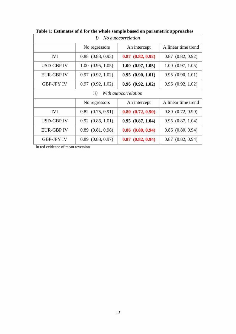
time trend. The results in Table 1 indicate that the time trend is not significant in any

case, the intercept being sufficient to describe the deterministic component of the

series. There is also evidence of mean reversion in some cases, namely for IVI (with

both autocorrelated and uncorrelated disturbances) as well as EUR-GBP IV and GBP-

JPY IV with autocorrelated disturbances, although the estimated values of d are

relatively high in all cases.

[Insert Tables 1 and 2 about here]

Next we apply a semi-parametric method (Robinson, 1995) that does not

require any assumptions on the behaviour of the error term. The results are displayed

8

in Table 2, which shows the estimated values for a selected group of bandwidth

parameters, m = 25, … (1), … (35), the results being very sensitive to the chosen

bandwidth. Here there is evidence of mean reversion in the case of IVI as well as

EUR-GBP IV for some bandwidth parameters; for GBP-USD IV and GBP-JPY IV

the estimated value of d is not statistically significantly different from 1.

Finally, we split the sample into two subsamples (before and after the Brexit

referendum), again using both parametric and semi-parametric methods. Table 3

displays the parametric results, distinguishing between the cases of uncorrelated

(Table 3i) and autocorrelated (Table 3ii) disturbances. In the latter case the estimated

value of d for IVI increases from 0.85 (which implies mean reversion) to 0.92

(suggesting lack of mean reversion since the unit root hypothesis cannot be rejected).

By contrast, the decrease in the degree of persistence observed for the IVs after the

break is not statistically significant. When allowing for autocorrelated disturbances,

the estimated value of d for IVI increases (from 0.78 to 0.83), and the same holds for

GBP-USD IV and EUR-GBP IV.

[Insert Table 3 and Figure 3 about here]

Finally, Figure 3 displays the semi-parametric estimates of d, before and after

the break, for all the possible bandwidth parameters. Consistently with the parametric

results, the evidence suggests an increase in the degree of persistence after the Brexit

referendum for IVI, GBP-USD IV and EUR-GBP IV, but not for GBP-JPY IV. In

other words, in the new economic environment created by the referendum there are

more long-lasting effects of shocks on market sentiment and investor fear, which

highlights the importance of completing swiftly the negotiations with the EU to agree

on the terms and conditions of Brexit and remove the existing (political) uncertainty.

9

At this stage concerns about economic growth and financial trading undoubtedly are

playing a role, and a well-structured Brexit deal would lessen if not eliminate them.

4. Conclusions

This paper examines the effects of Brexit on uncertainty in European financial

markets. More specifically, it applies (parametric and semi-parametric) fractional

integration methods to test for any changes of the degree of persistence of the FTSE

100 Implied Volatility Index (IVI) and of the British pound’s implied volatilities

(IVs) vis-à-vis the main currencies traded in the FOREX, namely the euro, the US

dollar and the Japanese yen.

Visual inspection of the data covering the period from the beginning of 2014

to the end of October 2017 suggests that the IVI reacted in anticipation of the Brexit

referendum and has been declining thereafter, whilst the British pound’s IVs have

remained above their initial level since the referendum. This evidence is consistent

with the fact that British firms with global outreach are in a better position to manage

the risk implied by the Brexit negotiations. On the other end, market participants seem

to feel the need to continue buying protection against future swings in the British

pound.

The econometric analysis provides evidence of a significant increase in the

persistence of all the series considered except the GBP-JPY IV, which indicates that

Brexit has had a noticeable impact (at least in the short run) on uncertainty. Since the

IVI and the British pound’s IVs can be interpreted as “investor fear gauge” (see

Whaley, 2000), it seems clear that investors have taken a dim view of the

consequences of Brexit, especially because of the prolonged political uncertainty

associated with this process and its uncertain future outcome, the “fear” factor

10

becoming more persistent as well as more sizeable in most cases and affecting

investment strategies. Although it is too early to express a view on the long-term

effects of Brexit (especially on the real economy), undoubtedly there has been a short-

term negative impact on financial markets. Achieving an appropriate Brexit deal in

the near future appears to be of paramount importance for the British economy.

11

References Baker, S.R., N. Bloom, and S.J. Davis, 2016a. "Measuring economic policy uncertainty," The Quarterly Journal of Economics, 131(4), 1593-1636. Baker, S.R., N. Bloom, and S.J. Davis, 2016b. “Policy uncertainty: Trying to estimate the uncertainty impact of brexit.” Presentation, September 2. http://www.policyuncertainty.com/media/Brexit_Discussion.pdf Bloomfield, P., 1973. “An exponential model in the spectrum of a scalar time series,” Biometrika, 60, 217-226. Capital Group, 2013. “Capital idea: Consider using economic exposure to map portfolios instead of country of domicile.” Investment Insights, London: Capital International Limited. https://fundspeople-repository.s3.amazonaws.com/system/audio_document/file/159/b35ec81d8c3f1149.pdf Caporale, G.M., L. Gil-Alana, and A. Plastun, 2017. “Is market fear persistent? A long-memory analysis”, WP no. 17-15, Department of Economics and Finance, Brunel University, London; also CESifo WP no. 6534 and DIW Berlin DP no. 1670. Chow, V., W. Jiang, and J. Li, 2014. “Does VIX truly measure return volatility?” West Virginia University, mimeo. Available at SSRN: https://ssrn.com/abstract=2489345 or http://dx.doi.org/10.2139/ssrn.2489345 Chow, V., W. Jiang, and J. Li, 2016. “VIX decomposition, the price of fear and stock return predictability,” West Virginia University, mimeo. Available at SSRN: https://ssrn.com/abstract=2747169. Corsi, F., 2009. “A simple approximate long memory model of realized volatility,” Journal of Financial Econometrics, 7, 174–196. Dahlhaus, R., 1989. “Efficient parameter estimation for self-similar processes,” Annals of Statistics, 17(4), 1749-1766. Fernandes M., M. C. Medeiros, and M. Scharth, 2014. “Modeling and predicting the CBOE market volatility index,” Journal of Banking and Finance, 40, 1-10. Fleming, J., B. Ostdiek, and R. E. Whaley, 1995, Predicting stock market volatility: A new measure,” Journal of Futures Markets, 15, 265–302. Gil-Alana, L.A., 2004. “The use of the model of Bloomfield (1973) as an approximation to ARMA processes in the context of fractional integration,” Mathematical and Computer Modelling, 39, 429-436. Giot, P., 2005. “Relationships between implied volatility indexes and stock index returns,” Journal of Portfolio Management, 26, 12-17.

12

Guo, H., and R. Whitelaw, 2006. “Uncovering the risk-return relationship in the stock market,” Journal of Finance, 61, 1433-1463. Heydon T., L. Ferreira, M. McArdle, and M. Antognelli, 2000. “Fear and greed in global asset allocation,” Journal of Investing, 9 (1), 27-35. Huskaj, B., 2013. “Long memory in VIX futures volatility,” Review of Futures Markets, 21(1), 31-48. Jo-Hui C. and H. Yu-Fang, 2014. “Memory and structural breaks in modelling the volatility dynamics of VIX-ETFS,” International Journal of Business, Economics and Law, 4, 1, 54-63. Kierzenkowski, R., N. Pain, E. Rusticelli, and S. Zwart, 2016. “The economic consequences of Brexit: A taxing decision,” OECD Economic Policy Papers 16, OECD Publishing. Koopman, S. J., B. Jungbacker, and E. Hol, 2005. “Forecasting daily variability of the S&P 100 stock index using historical, realised and implied volatility measurements,” Journal of Empirical Finance 12, 445–475. Philippon, T., 2016. “Brexit and the end of the Great Policy Moderation,” Brookings Papers on Economic Activity, 2, pp. 385-393. Robinson, P.M., 1994. “Efficient tests of nonstationary hypotheses,” Journal of the American Statistical Association, 89, 1420-1437. Robinson, P.M., 1995. “Gaussian semi-parametric estimation of long range dependence,” Annals of Statistics, 23, 1630-1661. Whaley, R., 2000. “The investor fear gauge,” Journal of Portfolio Management, 26, 12-17.

13

Table 1: Estimates of d for the whole sample based on parametric approaches i) No autocorrelation

No regressors An intercept A linear time trend

IVI 0.88 (0.83, 0.93) 0.87 (0.82, 0.92) 0.87 (0.82, 0.92)

USD-GBP IV 1.00 (0.95, 1.05) 1.00 (0.97, 1.05) 1.00 (0.97, 1.05)

EUR-GBP IV 0.97 (0.92, 1.02) 0.95 (0.90, 1.01) 0.95 (0.90, 1.01)

GBP-JPY IV 0.97 (0.92, 1.02) 0.96 (0.92, 1.02) 0.96 (0.92, 1.02)

ii) With autocorrelation

No regressors An intercept A linear time trend

IVI 0.82 (0.75, 0.91) 0.80 (0.72, 0.90) 0.80 (0.72, 0.90)

USD-GBP IV 0.92 (0.86, 1.01) 0.95 (0.87, 1.04) 0.95 (0.87, 1.04)

EUR-GBP IV 0.89 (0.81, 0.98) 0.86 (0.80, 0.94) 0.86 (0.80, 0.94)

GBP-JPY IV 0.89 (0.83, 0.97) 0.87 (0.82, 0.94) 0.87 (0.82, 0.94) In red evidence of mean reversion

14

Table 2: Estimates of d for the whole sample using semi-parametric approaches IVI IV USD-GBP IV EUR-GBP IV JPY-GBP

25 0.510 0.955 0.848 0.996 26 0.528 0.949 0.837 0.995 27 0.554 0.955 0.830 1.000 28 0.562 0.977 0.844 1.022 29 0.575 0.963 0.824 1.012 30 0.591 0.944 0.818 1.023 31 0.620 0.965 0.835 1.041 32 0.607 0.975 0.849 1.043 33 0.607 0.992 0.865 1.047 34 0.607 0.976 0.850 1.014 35 0.631 0.964 0.854 1.012

In red, evidence of mean reversion. In bold, evidence of unit roots.

15

Table 3: Estimates of d for the subsamples before and after the Brexit referendum based on parametric approaches

i) No autocorrelation

No regressors An intercept A linear time trend

IVI before 0.86 (0.80, 0.93) 0.85 (0.79, 0.92) 0.85 (0.79, 0.92)

IVI after 0.94 (0.88, 1.02) 0.92 (0.84, 1.00) 0.92 (0.84, 1.00)

USD-GBP IV before 0.93 (0.88, 0.99) 1.11 (1.03, 1.20) 1.11 (1.03, 1.20)

USD-GBP IV after 0.95 (0.88, 1.04) 1.03 (0.95, 1.12) 1.03 (0.95, 1.12)

EUR-GBP IV before 0.93 (0.87, 1.00) 1.11 (1.03, 1.20) 1.11 (1.03, 1.20)

EUR-GBP IV after 0.92 (0.85, 1.01) 0.97 (0.90, 1.07) 0.97 (0.90, 1.07)

GBP-JPY IV before 0.90 (0.86, 0.95) 1.06 (0.99, 1.15) 1.06 (0.99, 1.15)

GBP-JPY IV after 0.96 (0.89, 1.06) 0.94 (0.85, 1.04) 0.94 (0.87, 1.04)

ii) With autocorrelation

No regressors An intercept A linear time trend

IVI before 0.80 (0.68, 0.91) 0.78 (0.66, 0.91) 0.78 (0.66, 0.91)

IVI after 0.87 (0.76, 0.99) 0.83 (0.72, 1.01) 0.83 (0.71, 0.98)

USD-GBP IV before 0.94 (0.86, 1.07) 0.91 (0.82, 1.04) 0.90 (0.82, 1.04)

USD-GBP IV after 0.84 (0.74, 0.95) 0.91 (0.75, 1.08) 0.93 (0.81, 1.08)

EUR-GBP IV before 0.86 (0.78, 0.97) 0.89 (0.78, 1.06) 0.90 (0.78, 1.06)

EUR-GBP IV after 0.80 (0.71, 0.92) 0.87 (0.69, 1.05) 0.90 (0.77, 1.06)

GBP-JPY IV before 0.94 (0.88, 1.03) 0.90 (0.83, 1.02) 0.90 (0.82, 1.03)

GBP-JPY IV after 0.84 (0.74, 0.95) 0.62 (0.50, 0.87) 0.79 (0.68, 0.90)

16

Figure 1: The IVI and British pound’s IVs

The vertical red line corresponds to 23 June 2016, the date of the Brexit referendum. Figure 2: The UK EPU Index

The vertical red line corresponds to 23 June 2016, the date of the Brexit referendum. Source: the data are from Baker et al (2016a).

010

2030

1/1/20

14

1/1/20

15

1/1/20

16

1/1/20

17

1/1/20

18

ftse 100

IVI

510

1520

25

1/1/20

14

1/1/20

15

1/1/20

16

1/1/20

17

1/1/20

18

gbp-usd eur-gbpgbp-jpy

Pound's IVs0

500

1000

1500

2000

2500

01jan

2014

01jan

2015

01jan

2016

01jan

2017

01jan

2018

17

Figure 3: Estimates of d for each subsample using semi-parametric methods

IVI

USD-GBP IV

EUR-GBP IV

GBP-JPY IV

The estimated d prior to the Brexit referendum is in blue, the one after the Brexit referendum is in red

0

0,2

0,4

0,6

0,8

1

1,2

1,4

1,6

1,8

21 9 17 25 33 41 49 57 65 73 81 89 97 105 113 121 129 137 145 153 161 169 177 185 193 201

0,4

0,8

1,2

1,6

2

0,4

0,8

1,2

1,6

2

0

0,4

0,8

1,2

1,6

2

1 8 15 22 29 36 43 50 57 64 71 78 85 92 99 106 113 120 127 134 141 148 155 162 169