briefing paper no. 2 - office for budget responsibilityobr.uk/docs/dlm_uploads/briefing paper no2...

Briefing paper No. 2Estimating the output gap

April 2011

© Crown copyright 2011

You may re-use this information (not including logos) free of charge in any format or medium, under the terms of the Open Government Licence. To view this licence, visit http://www.nationalarchives.gov.uk/doc/open-government-licence/ or write to the Information Policy Team, The National Archives, Kew, London TW9 4DU, or e-mail: [email protected].

Any queries regarding this publication should be sent to us at: [email protected]

ISBN 978-1-84532-880-1 PU1180

1 Briefing paper No. 2

Estimating the output gap

Contents

Chapter 1 Introduction ......................................................................................... 3

Chapter 2 The OBR’s estimates of the output gap: an overview .............................. 5

Chapter 3 Aggregate composite estimates ............................................................ 9

Chapter 4 Principal components estimates .......................................................... 15

Chapter 5 Conclusion ........................................................................................ 21

Introduction



1 Introduction

1.1 The Office for Budget Responsibility has been tasked with producing economic and fiscal forecasts over a five year time horizon, and with using these forecasts to assess whether the government is on course to achieve the medium-term fiscal targets that it has set itself. Both require us to estimate the ‘output gap’, the difference between the current level of activity in the economy and the potential level it could sustain while keeping inflation stable.

1.2 This Briefing Note briefly sets out the three methods by which the output gap is usually estimated and then describes in detail the ‘cyclical indicators’ method that the OBR has used to date in its Economic and fiscal outlook publications. A forthcoming Briefing Note, which we plan to publish later this year, will set out more details of the approach and methodology we use to construct our overall economic forecast.

1.3 The two variants of the cyclical indicators method we use are refined from forecast to forecast, so readers should not assume that the precise variables and parameters set out here will remain unchanged in future publications. It is also important to bear in mind that these techniques are used to inform the judgement that the OBR makes about the size of the output gap in its central forecast, but that we do not apply them without question. We might make (and would clearly explain) a judgement that diverges from what they tell us if we felt that the weight of other evidence suggested that would be appropriate.

1.4 There is significant uncertainty around any estimate of the output gap and it would be unwise to base an assessment of economic prospects on the belief that any single approach will consistently deliver the ‘correct’ answer (even if we could be sure after the event what the correct answer was). So in our Economic and fiscal outlooks we are careful to describe how our central estimate of the output gap compares to those of other leading forecasters who may use different techniques. And we also use sensitivity analysis to estimate how the Government’s chances of hitting its targets would be affected if the output gap was larger or smaller than our central estimate and if it was to be closed more or less quickly.

1.5 Later this year we plan to publish a paper exploring the various methods of estimating the output gap in more detail, including a historical assessment of the output gap. (To date we have applied the techniques described in this paper only

Introduction

Briefing paper No.2 4 Estimating the output gap

back to the beginning of 2007.) In the meantime we would welcome comments on our current approach and alternatives.

1.6 Section 2 of this paper gives an overview of our need for output gap estimates and the cyclical indicator method of estimation that we focus on. Sections 3 and 4 describe the two main variants of this method that we use, the ‘aggregate composite estimates’ approach and the ‘principal components analysis’ approach respectively. Section 5 briefly concludes.

The OBR’s estimates of the output gap: an overview



2 The OBR’s estimates of the output gap: an overview

Methods of estimating the output gap 2.1 The output gap is the difference between the current level of output in the

economy and the potential level that could be supplied without putting upward or downward pressure on inflation. Estimating the output gap is difficult because we cannot observe the supply potential of the economy directly, even in retrospect.

2.2 The OBR needs to estimate the output gap in part because we have been asked to assess whether the Government is on course to achieve its ‘fiscal mandate’, a target requiring the current budget (the difference between government receipts and non-investment spending) to be in cyclically-adjusted balance at a rolling five-year horizon. The cyclically-adjusted current budget is that which would be recorded if the output gap was zero.

2.3 More fundamentally, we cannot assess the prospects for economic growth over a five-year period without taking some view – implicit or explicit – of the level of activity the economy can sustain, how that level is likely to change, and how far above or below that level the economy is currently operating. This means that some view of the likely evolution of potential output and the output gap would be necessary to judge progress towards any medium-term target for the public finances, not just a cyclically-adjusted one.

2.4 As we cannot observe the level of potential output directly, we have to estimate the size of the output gap from available indicators or from assumptions about the path of potential output. Estimating the output gap in real time is particularly difficult as changes in data may reflect movements in potential output, cyclical fluctuations, or both. Distinguishing between the underlying trend in potential output and cyclical fluctuations around it can be hard even once a much longer run of data becomes available.

2.5 The three most commonly used methods of estimating the output gap are:

Statistical filters: Statistical tools such as the Hodrick-Prescott and

Christiano-Fitzgerald filters can be used to extract a smoothed trend from



an output series. If the trend approximates the path of potential output, then the output gap can be measured as the gap between the trend and the actual level of output at any given time.

Production functions: Estimates of supply potential can be derived from assumptions about the potential level of factor inputs (capital and labour) and Total Factor Productivity, the efficiency with which factor inputs are used to produce output.

Cyclical indicators: This is the approach currently used by the OBR. A wide range of indicators of the cyclical position of the economy are used to inform an estimate of the current size of the output gap. These indicators include a variety of survey measures of spare capacity and recruitment difficulties, as well as ONS data, such as average earnings growth.

2.6 One advantage of using a cyclical indicator-based approach is that it does not

rely directly on estimates of output. Accordingly estimates of the output gap based on this approach are likely to be less susceptible to revisions to National Accounts data. In addition, estimating the output gap in this way does not require an estimate of what trend growth has been over the recent past, which would in turn require a quantitative judgement on the extent to which the recession had affected the economy’s supply potential. Such judgements are subject to significant uncertainty, particularly in the absence of a long run of data.

2.7 However, we recognise that it would be unwise to base an assessment of economic prospects on any single approach alone. So in forming a judgement we also assess how the estimates produced by the cyclical indicators method compares to those of other leading forecasters who may use different techniques, including those based on production function approaches and statistical filters.

The cyclical indicators method 2.8 Cyclical indicators need to be combined and weighted to produce an aggregate

output gap estimate. This is not straightforward: the indicators typically relate to different variables and are derived from different sources. Even when each series has been transformed into comparable units of measurement, it is not obvious how much weight should be given to each.

2.9 We use two approaches to combine the cyclical indicators:

‘aggregate composite’ estimates are based on a weighted average of survey indicators of capacity utilisation and recruitment difficulties, with the weights on each indicator based on factor income and sector shares. For




example, recruitment difficulties are weighted by the labour share of income, while survey indicators relating specifically to the service or manufacturing sectors are weighted according to the relevant sector shares. More information on this method is set out in Section 3.

the indicators can also be combined using ‘principal components analysis’, a statistical technique that enables the identification of the common determinant of a number of variables. Principal components analysis assigns weights to each of the variables according to the underlying properties of the dataset, rather than according to a priori information e.g. factor income or sector shares. Unlike aggregate composite estimates, the principal components estimates take into account ONS indicators of spare capacity as well as survey-based measures. Further information on this approach is set out in Section 4.

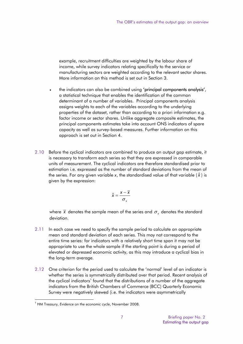
2.10 Before the cyclical indicators are combined to produce an output gap estimate, it

is necessary to transform each series so that they are expressed in comparable units of measurement. The cyclical indicators are therefore standardised prior to estimation i.e. expressed as the number of standard deviations from the mean of the series. For any given variable x, the standardised value of that variable ( x̂ ) is given by the expression:

x

xxx

ˆ

where x denotes the sample mean of the series and x denotes the standard deviation.

2.11 In each case we need to specify the sample period to calculate an appropriate

mean and standard deviation of each series. This may not correspond to the entire time series: for indicators with a relatively short time span it may not be appropriate to use the whole sample if the starting point is during a period of elevated or depressed economic activity, as this may introduce a cyclical bias in the long-term average.

2.12 One criterion for the period used to calculate the ‘normal’ level of an indicator is whether the series is symmetrically distributed over that period. Recent analysis of the cyclical indicators1 found that the distributions of a number of the aggregate indicators from the British Chambers of Commerce (BCC) Quarterly Economic Survey were negatively skewed (i.e. the indicators were asymmetrically

1 HM Treasury, Evidence on the economic cycle, November 2008.



distributed) in the period since the start of the series in 1989. This may reflect the fact that the series started near the local peak in GDP in the second quarter of 1990. The average of the entire span of the indicator will therefore tend to be biased by the fact that part of the up-phase of that economic cycle (i.e. the second half of the 1980s) will not be captured. By contrast, the BCC survey indicators generally showed stronger evidence of a normal distribution when the sample was restricted to the period from 1995.

2.13 To account for this, and to ensure a consistent approach across the cyclical indicators, most of the variables have been standardised using means and standard deviations based on the period since the first quarter of 1995. The exception to this is the set of indicators from the Bank of England Agent’s Summary of Business Conditions, which do not start until after 1995. These indicators have been standardised using means and standard deviation based on the period since the first quarter of 1998.

Aggregate composite estimates



3 Aggregate composite estimates

3.1 Aggregate composite estimates combine survey-based indicators of spare capacity using factor income and sector shares. This section sets out the underlying formulae used to construct these estimates. In all cases, the indicators have been standardised i.e. expressed in terms of standard deviations from their mean. References in the notation below to an indicator therefore correspond to the standardised version of that indicator.1 Table 3.1 provides a full summary of the indicators, the corresponding notation and the periods used to calculate the mean and standard deviation of each series.

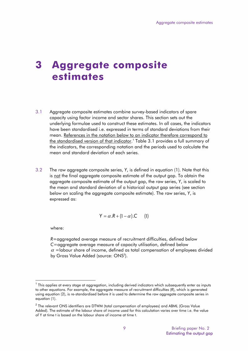
3.2 The raw aggregate composite series, Y, is defined in equation (1). Note that this

is not the final aggregate composite estimate of the output gap. To obtain the aggregate composite estimate of the output gap, the raw series, Y, is scaled to the mean and standard deviation of a historical output gap series (see section below on scaling the aggregate composite estimate). The raw series, Y, is expressed as:

)().(. 11 CRY

where:

R=aggregated average measure of recruitment difficulties, defined below C=aggregate average measure of capacity utilisation, defined below =labour share of income, defined as total compensation of employees divided by Gross Value Added (source: ONS2).

1 This applies at every stage at aggregation, including derived indicators which subsequently enter as inputs to other equations. For example, the aggregate measure of recruitment difficulties (R), which is generated using equation (2), is re-standardised before it is used to determine the raw aggregate composite series in equation (1). 2 The relevant ONS identifiers are DTWM (total compensation of employees) and ABML (Gross Value Added). The estimate of the labour share of income used for this calculation varies over time i.e. the value of Y at time t is based on the labour share of income at time t.



Aggregate measure of recruitment difficulties

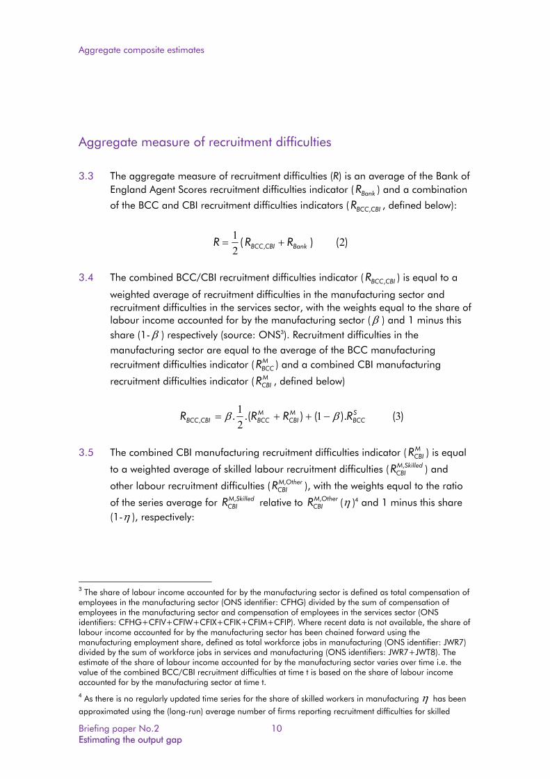
3.3 The aggregate measure of recruitment difficulties (R) is an average of the Bank of

England Agent Scores recruitment difficulties indicator ( BankR ) and a combination

of the BCC and CBI recruitment difficulties indicators ( CBIBCCR , , defined below):

)()( , 221

BankCBIBCC RRR

3.4 The combined BCC/CBI recruitment difficulties indicator ( CBIBCCR , ) is equal to a

weighted average of recruitment difficulties in the manufacturing sector and recruitment difficulties in the services sector, with the weights equal to the share of labour income accounted for by the manufacturing sector ( ) and 1 minus this share (1- ) respectively (source: ONS3). Recruitment difficulties in the manufacturing sector are equal to the average of the BCC manufacturing recruitment difficulties indicator ( M

BCCR ) and a combined CBI manufacturing

recruitment difficulties indicator ( MCBIR , defined below)

)().().(., 3121 S

BCCMCBI

MBCCCBIBCC RRRR

3.5 The combined CBI manufacturing recruitment difficulties indicator ( MCBIR ) is equal

to a weighted average of skilled labour recruitment difficulties ( SkilledMCBIR , ) and

other labour recruitment difficulties ( OtherMCBIR , ), with the weights equal to the ratio

of the series average for SkilledMCBIR , relative to OtherM

CBIR , ( )4 and 1 minus this share (1- ), respectively:

3 The share of labour income accounted for by the manufacturing sector is defined as total compensation of employees in the manufacturing sector (ONS identifier: CFHG) divided by the sum of compensation of employees in the manufacturing sector and compensation of employees in the services sector (ONS identifiers: CFHG+CFIV+CFIW+CFIX+CFIK+CFIM+CFIP). Where recent data is not available, the share of labour income accounted for by the manufacturing sector has been chained forward using the manufacturing employment share, defined as total workforce jobs in manufacturing (ONS identifier: JWR7) divided by the sum of workforce jobs in services and manufacturing (ONS identifiers: JWR7+JWT8). The estimate of the share of labour income accounted for by the manufacturing sector varies over time i.e. the value of the combined BCC/CBI recruitment difficulties at time t is based on the share of labour income accounted for by the manufacturing sector at time t. 4 As there is no regularly updated time series for the share of skilled workers in manufacturing has been

approximated using the (long-run) average number of firms reporting recruitment difficulties for skilled




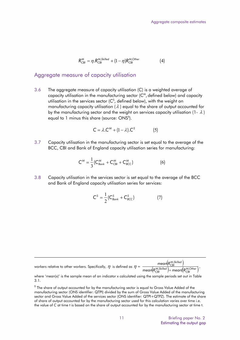
)()(. ,, 41 OtherMCBI

SkilledMCBI

MCBI RRR

Aggregate measure of capacity utilisation

3.6 The aggregate measure of capacity utilisation (C) is a weighted average of

capacity utilisation in the manufacturing sector (CM, defined below) and capacity utilisation in the services sector (CS, defined below), with the weight on manufacturing capacity utilisation ( ) equal to the share of output accounted for by the manufacturing sector and the weight on services capacity utilisation (1- ) equal to 1 minus this share (source: ONS5).

)().(. 51 SM CCC

3.7 Capacity utilisation in the manufacturing sector is set equal to the average of the BCC, CBI and Bank of England capacity utilisation series for manufacturing:

)()( 631 M

BCCMCBI

MBank

M CCCC

3.8 Capacity utilisation in the services sector is set equal to the average of the BCC and Bank of England capacity utilisation series for services:

)()( 721 S

BCCSBank

S CCC

workers relative to other workers. Specifically, is defined as =

OtherMCBI

SkilledMCBI

SkilledMCBI

RmeanRmean

Rmean,,

,

(,

where ‘mean(x)’ is the sample mean of an indicator x calculated using the sample periods set out in Table 3.1. 5 The share of output accounted for by the manufacturing sector is equal to Gross Value Added of the manufacturing sector (ONS identifier: QTPI) divided by the sum of Gross Value Added of the manufacturing sector and Gross Value Added of the services sector (ONS identifier: QTPI+QTPZ). The estimate of the share of share of output accounted for by the manufacturing sector used for this calculation varies over time i.e. the value of C at time t is based on the share of output accounted for by the manufacturing sector at time t.



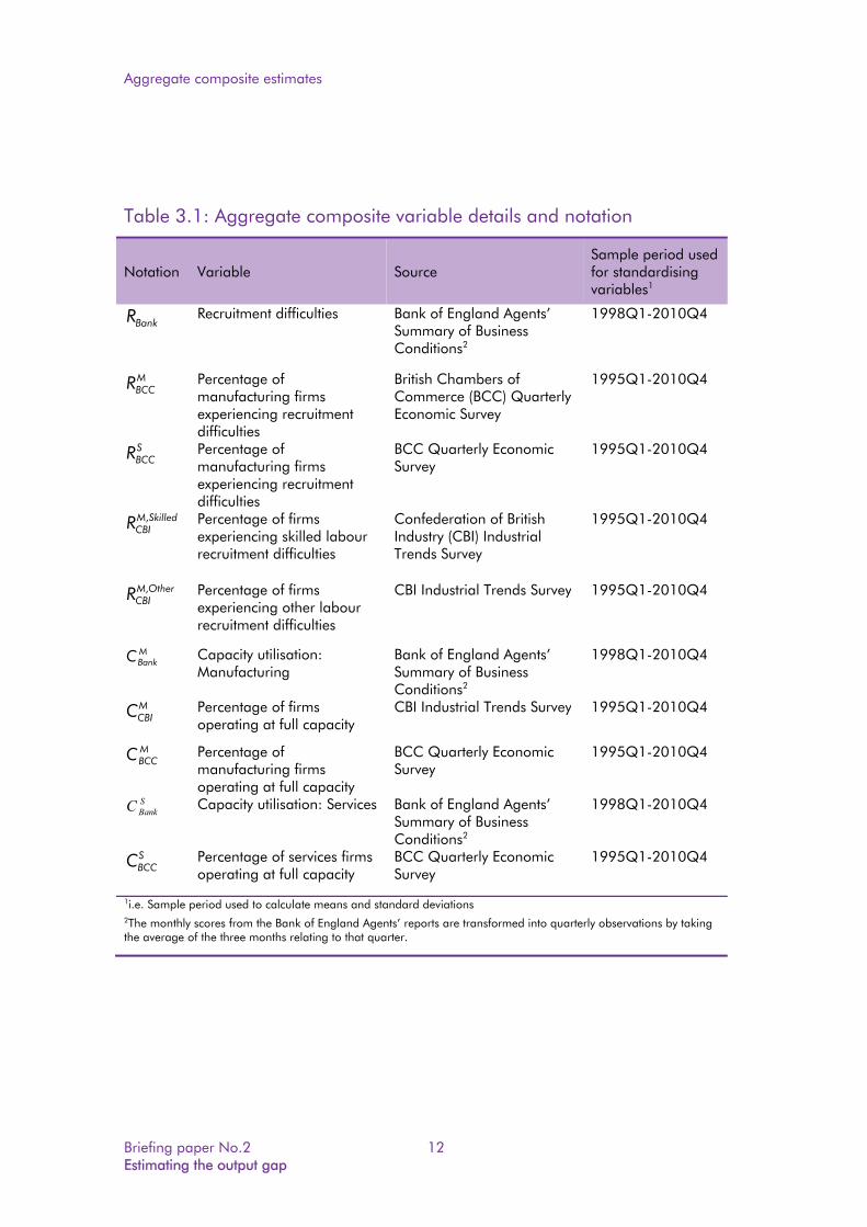
Table 3.1: Aggregate composite variable details and notation

Notation Variable Source Sample period used for standardising variables1

Recruitment difficulties Bank of England Agents’ Summary of Business Conditions2

1998Q1-2010Q4

Percentage of manufacturing firms experiencing recruitment difficulties

British Chambers of Commerce (BCC) Quarterly Economic Survey

1995Q1-2010Q4


BCC Quarterly Economic Survey

1995Q1-2010Q4

Percentage of firms experiencing skilled labour recruitment difficulties

Confederation of British Industry (CBI) Industrial Trends Survey

1995Q1-2010Q4

Percentage of firms experiencing other labour recruitment difficulties

CBI Industrial Trends Survey 1995Q1-2010Q4

Capacity utilisation: Manufacturing

Bank of England Agents’ Summary of Business Conditions2

1998Q1-2010Q4

Percentage of firms operating at full capacity

CBI Industrial Trends Survey 1995Q1-2010Q4

Percentage of manufacturing firms operating at full capacity


1995Q1-2010Q4

Capacity utilisation: Services Bank of England Agents’ Summary of Business Conditions2

1998Q1-2010Q4

Percentage of services firms operating at full capacity


1995Q1-2010Q4

1i.e. Sample period used to calculate means and standard deviations2The monthly scores from the Bank of England Agents’ reports are transformed into quarterly observations by taking the average of the three months relating to that quarter.

MBCCR

SBCCR

SkilledMCBIR ,

OtherMCBIR ,

MBankC

MCBIC

MBCCC

SBankC

BankR

SBCCC




Scaling the aggregate composite estimate

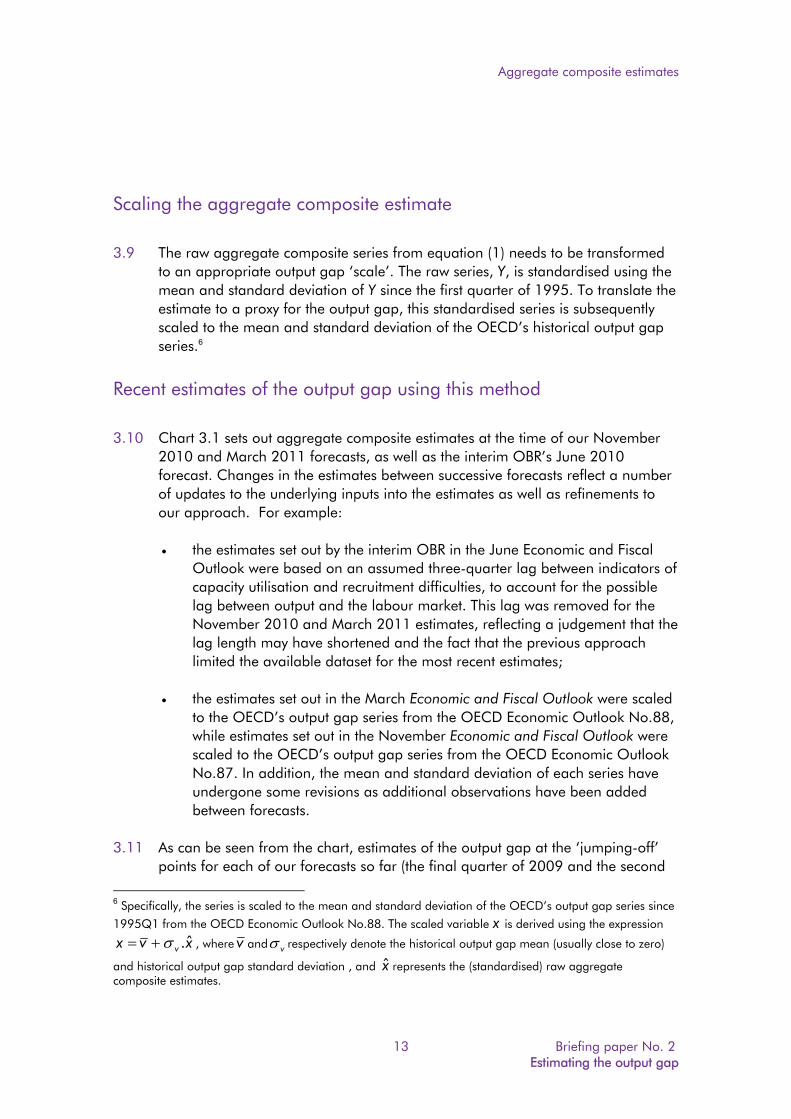
3.9 The raw aggregate composite series from equation (1) needs to be transformed

to an appropriate output gap ‘scale’. The raw series, Y, is standardised using the mean and standard deviation of Y since the first quarter of 1995. To translate the estimate to a proxy for the output gap, this standardised series is subsequently scaled to the mean and standard deviation of the OECD’s historical output gap series.6

Recent estimates of the output gap using this method

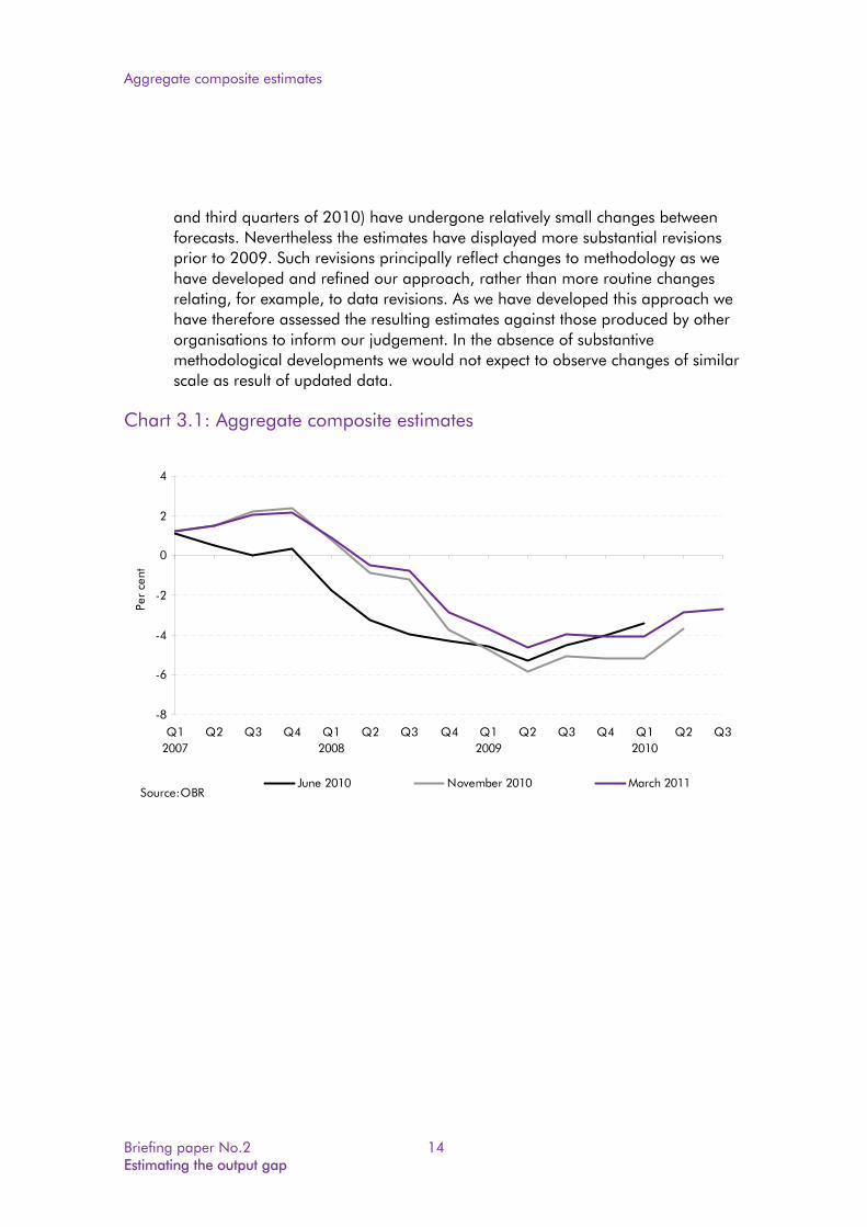
3.10 Chart 3.1 sets out aggregate composite estimates at the time of our November

2010 and March 2011 forecasts, as well as the interim OBR’s June 2010 forecast. Changes in the estimates between successive forecasts reflect a number of updates to the underlying inputs into the estimates as well as refinements to our approach. For example:

the estimates set out by the interim OBR in the June Economic and Fiscal Outlook were based on an assumed three-quarter lag between indicators of capacity utilisation and recruitment difficulties, to account for the possible lag between output and the labour market. This lag was removed for the November 2010 and March 2011 estimates, reflecting a judgement that the lag length may have shortened and the fact that the previous approach limited the available dataset for the most recent estimates;

the estimates set out in the March Economic and Fiscal Outlook were scaled to the OECD’s output gap series from the OECD Economic Outlook No.88, while estimates set out in the November Economic and Fiscal Outlook were scaled to the OECD’s output gap series from the OECD Economic Outlook No.87. In addition, the mean and standard deviation of each series have undergone some revisions as additional observations have been added between forecasts.

3.11 As can be seen from the chart, estimates of the output gap at the ‘jumping-off’ points for each of our forecasts so far (the final quarter of 2009 and the second

6 Specifically, the series is scaled to the mean and standard deviation of the OECD’s output gap series since

1995Q1 from the OECD Economic Outlook No.88. The scaled variable x is derived using the expression

xvx v ˆ. , where v and v respectively denote the historical output gap mean (usually close to zero)

and historical output gap standard deviation , and x̂ represents the (standardised) raw aggregate composite estimates.



and third quarters of 2010) have undergone relatively small changes between forecasts. Nevertheless the estimates have displayed more substantial revisions prior to 2009. Such revisions principally reflect changes to methodology as we have developed and refined our approach, rather than more routine changes relating, for example, to data revisions. As we have developed this approach we have therefore assessed the resulting estimates against those produced by other organisations to inform our judgement. In the absence of substantive methodological developments we would not expect to observe changes of similar scale as result of updated data.

Chart 3.1: Aggregate composite estimates

-8

-6

-4

-2

0

2

4

Q12007

Q2 Q3 Q4 Q12008

Q2 Q3 Q4 Q12009

Q2 Q3 Q4 Q12010

Q2 Q3

Per

cent

June 2010 November 2010 March 2011Source:OBR

Principal components estimates



4 Principal components estimates

4.1 Principal components analysis (PCA) is a commonly used statistical technique that enables the identification of the common determinant of a number of variables. In the case of a set of cyclical indicators, the PCA technique can be used to distinguish the common cyclical component from other components (such as the trend) of a set of indicators. To do this, PCA chooses the weights (also referred to as ‘loadings’) for each indicator. 1 The combination of indicators based on these weights can then be used to construct a series for the output gap.

4.2 Principal components analysis estimates are generated by statistical methods and can be computed using specialist statistical/econometric software, such as E-Views or STATA.2 Note that unlike the aggregate composite estimates, the weights on different indicators in PCA approach are determined ‘statistically’ (i.e. according to the properties of the dataset), rather than being imposed from a priori information (e.g. sector/factor income shares). One advantage of this is that PCA can used to combine a variety of different types of indicator where a priori information on appropriate weights may not exist (e.g. the relative weight of ONS indicators compared to survey-based measures).

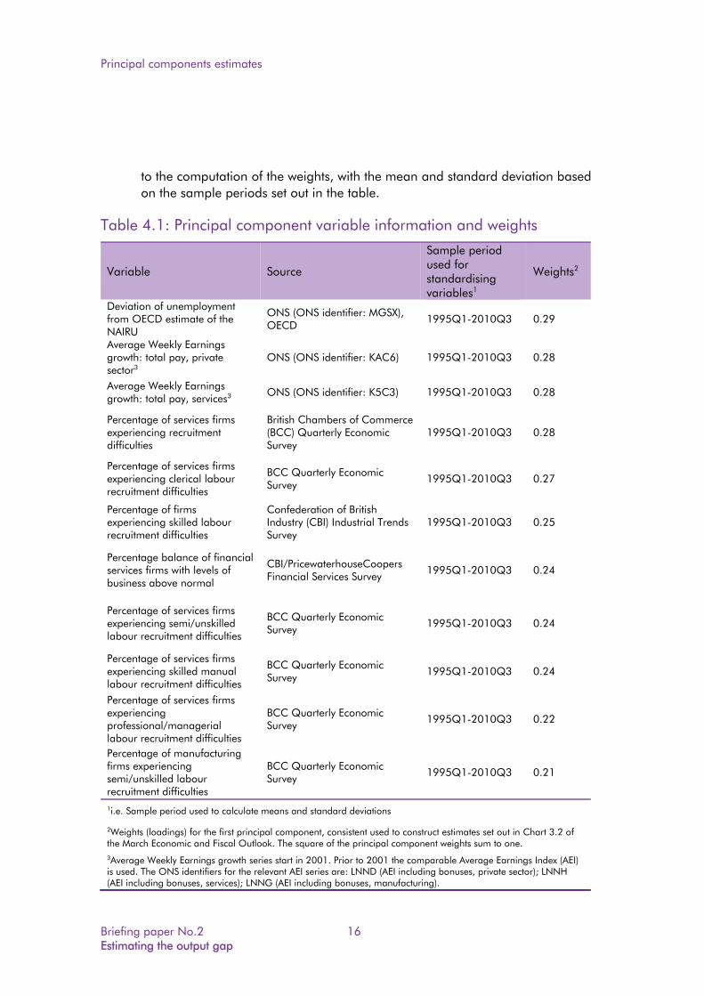
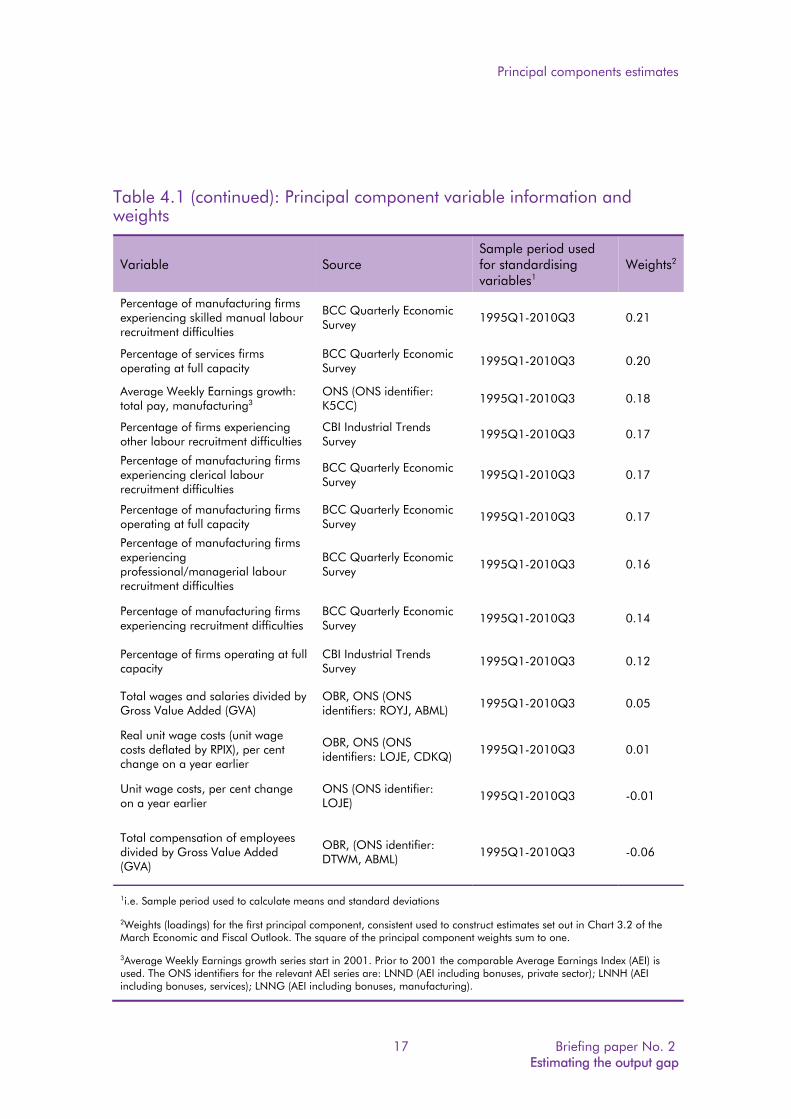
4.3 Table 4.1 sets out the variables used in the principal component estimates, along with the derived weights on each indicator. The variables are standardised prior

1 Principal components analysis specifies a number of different linear combinations of the underlying variables which (i) are uncorrelated with each other; and (ii) contain the maximum variance. The first principal component is the linear combination which has the greatest variance. This component is interpreted as a proxy for the output gap as it is assumed that the output gap is the most important common determinant of the cyclical indicators. 2 The STATA command (based on STATA version 11.1) used to generate the PCA estimates set out here is ‘PCA [VAR], components(1) covariance’, where’[VAR]’ is the list of variable names, ‘components(1)’ denotes the command to retain only the first component and ‘covariance’ denotes the use of the covariance matrix . This command can also be selected from the drop-down menu at Statistics/Multivariate analysis/Factor and principal component analysis/Principal Component Analysis. The PCA command produces the weights (or loadings) for the first principal component. The weighted combination of the PCA variables using these weights i.e. the raw PCA output used to construct the output gap estimates, are referred to as the ‘PCA scores’ and can be retrieved using the post-estimation command ‘predict [VARNAME], score’, where ‘[VARNAME]’ is the user-assigned name to the output series. This command can also be selected from the drop-down menu at Statistics/Postestimation/Predictions, residuals etc..., and selecting the option ‘Scores based on the components (default)’.



to the computation of the weights, with the mean and standard deviation based on the sample periods set out in the table.

Table 4.1: Principal component variable information and weights

Variable Source

Sample period used for standardising variables1

Weights2

Deviation of unemployment from OECD estimate of the NAIRU

ONS (ONS identifier: MGSX), OECD

1995Q1-2010Q3 0.29

Average Weekly Earnings growth: total pay, private sector3

ONS (ONS identifier: KAC6) 1995Q1-2010Q3 0.28

Average Weekly Earnings growth: total pay, services3

ONS (ONS identifier: K5C3) 1995Q1-2010Q3 0.28

Percentage of services firms experiencing recruitment difficulties

British Chambers of Commerce (BCC) Quarterly Economic Survey

1995Q1-2010Q3 0.28

Percentage of services firms experiencing clerical labour recruitment difficulties


1995Q1-2010Q3 0.27

Percentage of firms experiencing skilled labour recruitment difficulties

Confederation of British Industry (CBI) Industrial Trends Survey

1995Q1-2010Q3 0.25

Percentage balance of financial services firms with levels of business above normal

CBI/PricewaterhouseCoopers Financial Services Survey

1995Q1-2010Q3 0.24

Percentage of services firms experiencing semi/unskilled labour recruitment difficulties


1995Q1-2010Q3 0.24

Percentage of services firms experiencing skilled manual labour recruitment difficulties


1995Q1-2010Q3 0.24

Percentage of services firms experiencing professional/managerial labour recruitment difficulties


1995Q1-2010Q3 0.22

Percentage of manufacturing firms experiencing semi/unskilled labour recruitment difficulties


1995Q1-2010Q3 0.21

1i.e. Sample period used to calculate means and standard deviations 2Weights (loadings) for the first principal component, consistent used to construct estimates set out in Chart 3.2 of the March Economic and Fiscal Outlook. The square of the principal component weights sum to one. 3Average Weekly Earnings growth series start in 2001. Prior to 2001 the comparable Average Earnings Index (AEI) is used. The ONS identifiers for the relevant AEI series are: LNND (AEI including bonuses, private sector); LNNH (AEI including bonuses, services); LNNG (AEI including bonuses, manufacturing).




Table 4.1 (continued): Principal component variable information and weights

Variable Source Sample period used for standardising variables1

Weights2

Percentage of manufacturing firms experiencing skilled manual labour recruitment difficulties


1995Q1-2010Q3 0.21

Percentage of services firms operating at full capacity


1995Q1-2010Q3 0.20

Average Weekly Earnings growth: total pay, manufacturing3

ONS (ONS identifier: K5CC) 1995Q1-2010Q3 0.18

Percentage of firms experiencing other labour recruitment difficulties

CBI Industrial Trends Survey

1995Q1-2010Q3 0.17

Percentage of manufacturing firms experiencing clerical labour recruitment difficulties


1995Q1-2010Q3 0.17

Percentage of manufacturing firms operating at full capacity


1995Q1-2010Q3 0.17

Percentage of manufacturing firms experiencing professional/managerial labour recruitment difficulties


1995Q1-2010Q3 0.16



1995Q1-2010Q3 0.14

Percentage of firms operating at full capacity

CBI Industrial Trends Survey

1995Q1-2010Q3 0.12

Total wages and salaries divided by Gross Value Added (GVA)

OBR, ONS (ONS identifiers: ROYJ, ABML) 1995Q1-2010Q3 0.05

Real unit wage costs (unit wage costs deflated by RPIX), per cent change on a year earlier

OBR, ONS (ONS identifiers: LOJE, CDKQ)

1995Q1-2010Q3 0.01

Unit wage costs, per cent change on a year earlier

ONS (ONS identifier: LOJE)

1995Q1-2010Q3 -0.01

Total compensation of employees divided by Gross Value Added (GVA)

OBR, (ONS identifier: DTWM, ABML)

1995Q1-2010Q3 -0.06

1i.e. Sample period used to calculate means and standard deviations 2Weights (loadings) for the first principal component, consistent used to construct estimates set out in Chart 3.2 of the March Economic and Fiscal Outlook. The square of the principal component weights sum to one.

3Average Weekly Earnings growth series start in 2001. Prior to 2001 the comparable Average Earnings Index (AEI) is used. The ONS identifiers for the relevant AEI series are: LNND (AEI including bonuses, private sector); LNNH (AEI including bonuses, services); LNNG (AEI including bonuses, manufacturing).



4.4 The ‘raw’ series, X, from the principal component analysis can then be written as:

)(81

i

n

iiZX

4.5 where iZ denotes the (standardised) cyclical indicator and i the weight (or

‘loading’) corresponding to that indicator, as set out in Table 4.1; i.e. the series X represents a linear combination of the cyclical indicators.

4.6 As with the ‘aggregate composite’ estimates the raw output from the principal components analysis is transformed to make the results meaningful. The raw series, X, is standardised using the mean and standard deviation of X since the first quarter of 1995. To translate the estimate to a proxy for the output gap, this standardised series is subsequently scaled to the mean and standard deviation of the OECD’s historical output gap series.3

4.7 The resulting series produced by this approach can be relatively volatile, which is likely to reflect the fact that principal components analysis aims to find combinations of the variables with the greatest variance. A three-quarter moving average is therefore applied to the series to adjust for the volatility of the series.

Recent estimates of the output gap using this method

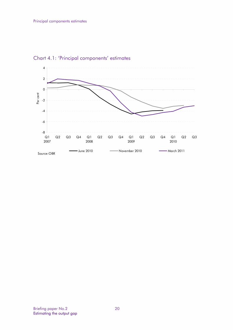
4.8 Chart 4.1 sets out principal components estimates at the time of our November 2010 and March 2011 forecasts, as well as the interim OBR’s June 2010 forecast. Changes in the estimates between successive forecasts reflect both refinements to methodology and changes to the underlying data. For example:

a four-quarter backward moving average was used for the estimates presented in the November Economic and Fiscal Outlook. This was refined to a three-quarter centred moving average in the March Outlook as this was judged to provide a better balance between adjusting for the volatility of the series and retaining information from the underlying data;

as with the aggregate composite estimates, the principal component estimates set out by the interim OBR in the June Economic and Fiscal Outlook were based on an assumed three-quarter lag for a number of labour market variables. This lag was removed for the November 2010 and

3 Specifically, the series is scaled to the mean and standard deviation of the OECD’s output gap series since

1995Q1 from the OECD Economic Outlook No.88. The scaled variable x is derived using the expression

xvx v ˆ. , where v and v respectively denote the historical output gap mean (usually close to zero)

and historical output gap standard deviation , and x̂ represents the (standardised) raw principal components estimates.




March 2011 estimates, reflecting a judgement that the lag length may have shortened and the fact that the previous approach limited the available dataset for the most recent estimates;

the estimates set out in the March Economic and Fiscal Outlook were scaled to the OECD’s output gap series from the OECD Economic Outlook No.88, while estimates set out in the November Economic and Fiscal Outlook were scaled to the OECD’s output gap series from the OECD Economic Outlook No.87. The scaling procedure was also modified between successive updates,4 while the mean and standard deviation of each series have undergone some revisions as additional observations have been added between forecasts;

for the estimates presented in the interim November Economic and Fiscal Outlook, the principal components estimates were based on a number of Average Earnings Index (AEI) series. The Average Earnings Index has since been discontinued by the ONS and replaced by the Average Weekly Earnings (AWE) series as the headline indicator of earnings growth. The estimates set out in the March Economic and Fiscal Outlook were therefore based on AWE series rather than AEI series (see Table 4.1).

4.9 As with the aggregate composite estimates, estimates of the output gap at the ‘jumping-off’ points for each of our forecasts so far (the final quarter of 2009 and the second and third quarters of 2010) have undergone relatively small changes between forecasts, although the estimates have displayed more substantial revisions prior to 2009. Again, such revisions principally reflect changes to methodology as we have developed and refined our approach, rather than more routine changes relating, for example, to data revisions. In the absence of substantive methodological developments we would not expect to observe changes of similar scale as result of updated data.

4 Specifically, for the March 2011 estimates the raw output was scaled according to the

expression xvx v ˆ. , with notation as set out in footnote 3, while for the June 2010 and November

2010 the raw output was scaled using the procedure vvxx /)ˆ( . This modification meant that the

procedure used to scale the March 2011 principal component estimates was consistent with the procedure used to scale the ‘aggregate composite’ estimates (see section 3).



Chart 4.1: ‘Principal components’ estimates

-8

-6

-4

-2

0

2

4

Q12007

Q2 Q3 Q4 Q12008

Q2 Q3 Q4 Q12009

Q2 Q3 Q4 Q12010

Q2 Q3

Per

cent

June 2010 November 2010 March 2011Source:OBR

Conclusion



5 Conclusion

5.1 The Office for Budget Responsibility has been tasked with producing economic and fiscal forecasts over a five year time horizon, and with using these forecasts to assess whether the government is on course to achieve the medium-term fiscal targets that it has set itself. Both require us to estimate the ‘output gap’, the difference between the current level of activity in the economy and the potential level it could sustain while keeping inflation stable.

5.2 There are a number of different approaches to estimating the output gap. Our approach is based on estimating the output gap using contemporaneous indicators of spare capacity, although we also assess how the estimates produced by this method compares to those of other leading forecasters who may use different approaches. We also use sensitivity analysis to estimate how the Government’s chances of hitting its targets would be if the output gap differed from our central estimate.

5.3 The methods set out in this note are refined from forecast to forecast, so the exact variables and techniques set out in this note may be subject to change. Revisions to estimates between successive forecasts have reflected a number of changes to methodology as we have refined and developed our approach. It should also be borne in mind that the estimates produced by these methods form part one of the factors that inform our judgement, alongside estimates produced by other organisations using different techniques.

5.4 Despite various changes to variables and methods, we have not changed the central judgements we have made for the ‘jumping off’ quarters for each forecast. These include the judgement that the output gap was around -4 per cent in the final quarter of 2009; and around -3½ per cent and -3¼ per cent in the second and third quarters of 2010 respectively.

5.5 Later this year we plan to publish a paper exploring various methods of estimating the output gap in more detail, including a historical assessment of the output gap. In the meantime, we would welcome comments on methodology or alternatives. A forthcoming Briefing Note will also put our approach to the output gap into the broader context of our overall approach to the economic forecast.

briefing paper no. 2 - office for budget responsibilityobr.uk/docs/dlm_uploads/briefing paper no2...

Documents