broad-scale geographical evolution of ferns marc
TRANSCRIPT

BROAD-SCALE GEOGRAPHICAL EVOLUTION OF FERNS
Marc David Bogonovich
Submitted to the faculty of the University Graduate School
in partial fulfillment of the requirements
for the degree
Doctor of Philosophy
in the Department of Biology,
Indiana University
December 2012

ii
Accepted by the Graduate Faculty, Indiana University, in partial fulfillment of the requirements
for the degree of Doctor of Philosophy.
Doctoral Committee
_____________________________
Maxine Watson, Ph.D.
_____________________________
James Bever, Ph.D.
_____________________________
Leonie Moyle, Ph.D.
_____________________________
Scott Robeson, Ph.D.
August 29th, 2011

iii
Copyright © 2012
Marc David Bogonovich

iv
To my parents, David and Sheila Bogonovich

v
Acknowledgements
I thank Maxine Watson, my advisor, for her continual support and guidance. I also thank
my committee members, James Bever, Leonie Moyle, and Scott Robeson for their attention,
collaboration, and excellent feedback. Michael Tansey was a valuable mentor. I thank Gretchen
Clearwater for her patience and sense of humor. I gratefully acknowledge the support of the
Floyd fellowship.
I would like to thank collaborator Michael Barker for his enthusiasm for ferns and
lycophytes. Bever lab members provided endless feedback and company. Heather Reynolds and
Keith Clay were original committee members. Stephen Friesen provided critical feedback that
greatly influenced the conceptual structure of this dissertation in its final year. The members of
the Watson lab, Immaculate Kyampeire, Erica Waters, and Timothy Griffith, deserve my
gratitude. The following individuals helped in many different ways. Caroline Angelard, Marina
Antonio, Collin Hobbes, Daniel Johnson, Elizabeth Koziol, Kerry Woods, and my students
Taylor Wahlig, Kevin Sapp, Tara Florida, and Josh Pecenica.
Most importantly I would like to thank my family and close friends. These people include
my friends Mary Damm, Jason Dolmetsch, and Matthew Rhodes, my parents David and Sheila
Bogonovich, grandparents Victor and Marion Lalli and George and Madeline Bogonovich, and
my sisters Megan and Meredith Bogonovich.

vi
Marc David Bogonovich
Broad-scale geographical evolution of ferns
In this dissertation I explore broad-scale regularities in the distribution of North American
ferns and lycophytes. I test models for the evolution of these regularities. To this end, I construct
a comprehensive database of all North American fern and lycophyte species. In the final
empirical chapter I extend my analyses to New World mammals and global amphibians.
First, I describe patterns of North American fern and lycophyte species and family
richness and describe the relationships of these patterns with climate. Next, I explore the
geography of fern polyploid species and present biogeographical evidence that most polyploid
speciation events are evolutionary dead-ends. These results contrast with notions that polyploid
speciation leads to evolutionary novelty and adaptive geographical expansion. Next, I test the
“Out of The Tropics” model (OTT) for the evolution of latitudinal gradients in diversity. The
OTT model proposes that higher taxa tend to originate in the tropics, and subsequently expand
into temperate regions while maintaining a tropical presence. The OTT model predicts that older
and diverse higher taxa will have expanded from their region of tropical origin, while younger
and less diverse higher taxa will still be located in the tropics. I find partial support for the OTT
model. Endemic fern families are found only in the tropics suggesting fern families more
frequently originate in the tropics than the extra-tropics. Fern families with many species extend
further into temperate regions than do less diverse families. However, family age is not
correlated with the degree of extension from the tropics.
In the final empirical chapter, I describe a global biogeographical rule observed in ferns,
mammals and amphibians. The new rule states that diversity of a taxon at the taxon's richness
peak predicts the amount of geographical expansion of that taxon from its center, and the number

vii
of species completely outside the taxon's center. I call these patterns diversity-expansion
relationships, and I explore these patterns using multiple measures of diversity and geographical
breadth (expansion). I propose alternative explanations for the existence of diversity-expansion
patterns and discuss their macroevolutionary implications.
______________________________
______________________________
______________________________
______________________________

viii
Table of contents
Section Page
Dedication......................................................................................................................................iv
Acknowledgments..........................................................................................................................v
Abstract..........................................................................................................................................vi
List of Tables...................................................................................................................................x
List of Figures................................................................................................................................xi
Chapter 1. Introduction............................................................................................................1
Chapter 2. Patterns of North American fern and lycophyte richness at three taxonomic
levels Abstract..................................................................................................................12
Introduction............................................................................................................12
Methods..................................................................................................................17
Results....................................................................................................................21
Discussion..............................................................................................................24
Figures and Tables..................................................................................................32
Chapter 3. Biogeography of North American fern polyploid species Abstract..................................................................................................................42
Introduction............................................................................................................43
Methods..................................................................................................................47
Results....................................................................................................................50
Discussion..............................................................................................................52
Figures and Tables..................................................................................................58
Chapter 4. Using species elevation data and range maps to infer thermal niche range of
North American fern and lycophyte families Abstract..................................................................................................................68
Introduction............................................................................................................69
Methods..................................................................................................................71
Results....................................................................................................................75
Discussion..............................................................................................................76
Figures....................................................................................................................78

ix
Table of contents, continued
Section Page
Chapter 5. The Russian doll pattern: A test of the Out of the Tropics (OTT) hypothesis
with North American ferns Abstract..................................................................................................................83
Introduction............................................................................................................84
Methods..................................................................................................................87
Results....................................................................................................................90
Discussion..............................................................................................................92
Figures and Equations............................................................................................96
Chapter 6. The relationship between taxon richness and geographical breadth: a
biogeographical rule
Abstract................................................................................................................103
Introduction..........................................................................................................103
Methods................................................................................................................107
Results..................................................................................................................111
Discussion............................................................................................................114
Figures and Tables................................................................................................120
Chapter 7. Discussion Geography as a Lens for Macroevolution............................................................135
Diversity-Expansion Patterns in Historical Context............................................141
Final Thoughts.....................................................................................................144
References...................................................................................................................................145
Curriculum vitae........................................................................................................................161

x
List of Tables
Chapter 1.
none
Chapter 2.
Table 2.1 Chapter 2 climate variables and sources.
Table 2.2 R-squared values and equation coefficients for regressions climate and
Monilophyte richness.
Chapter 3.
Table 3.1 Summary of variables and their sources for Chapter 3.
Table 3.2 R-squared values for correlations presented in Chapter 3.
Chapter 4.
none
Chapter 5.
none
Chapter 6.
Table 6.1 Variables used to represent diversity and geographical breadth (expansion) of
higher taxa.
Table 6.2 Taxon thermal variables. Variables used in Chapter 6 to describe the thermal niche
of higher taxa.
Chapter 7.
none

xi
List of Figures
Chapter 1.
none
Chapter 2.
Figure 2.1 (a) Fern species richness. (b) Fern genus richness. (c) Fern family richness. (d)
Map of residuals of the regression of fern family richness on mean annual
temperature (MAT), annual rainfall (RAN), and precipitation seasonality (Bio15).
(e) Pteridophyte (ferns and lycophytes) species richness. (f) Lycophyte species
richness.
Figure 2.2 (a) Binned scatter plot of family richness in North America with actual
evapotranspiration (AET) on the x-axis and mean annual temperature is on the y-
axis (MAT). (b) Similar to Figure 2.2a, except that annual rainfall (RAN) is
represented on the x-axis rather than AET.
Figure 2.3 Species richness maps of fern and lycophyte families. (a) Anemiaceae. (b)
Aspleniaceae. (c) Blechnaceae. (d) Dennstaedtiaceae. (e) Dryopteridaceae. (f)
Equisetaceae.
Figure 2.4 Species richness maps of fern and lycophytes families. (a) Gleicheniaceae. (b)
Hymenophyllaceae. (c) Isoetaceae. (d) Lindsaeaceae. (e) Lomariopsidaceae. (f)
Lycopodiaceae.
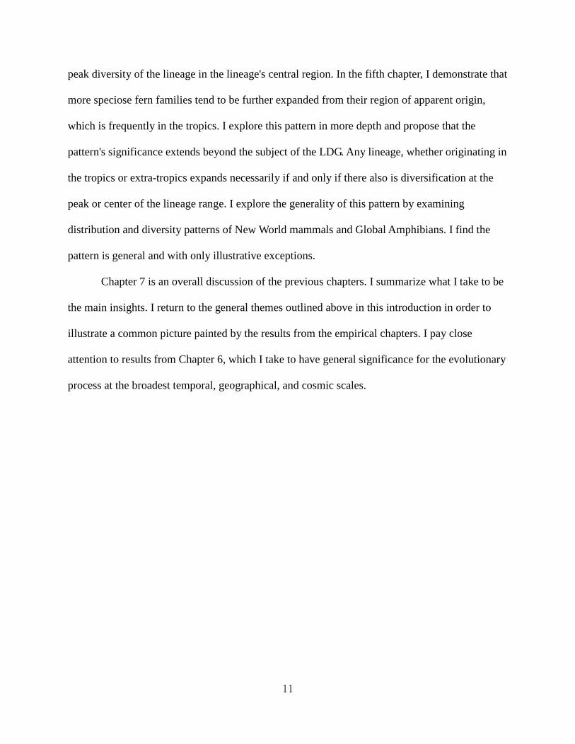
Figure 2.5 Species richness maps of fern and lycophytes families. (a) Lygodiaceae. (b)
Marsileaceae. (c) Onocleaceae. (d) Ophioglossaceae. (e) Osmundaceae. (f)
Polypodiaceae.
Figure 2.6 Species richness maps of fern and lycophytes families. (a) Psilotaceae. (b)
Pteridaceae. (c) Salviniaceae. (d) Schizaeaceae. (e) Selaginellaceae. (f)
Tectariaceae.
Figure 2.7 Species richness maps of fern and lycophytes families. (a) Thelypteridaceae. (b)
Woodsiaceae.
Chapter 3.
Figure 3.1 Hypothetical relationships between polyploid potential and tetraploid richness.
Figure 3.2 Monilophyte species richness.
Figure 3.3 Frequency histogram of ploidy level of species within the study region.
Figure 3.4 Percent of monilophytes that are tetraploid.
Figure 3.5 Mean chromosome number of monilophytes.
Figure 3.6 Median chromosome number of monilophytes.
Figure 3.7 Scatter plot of mean chromosome number of monilophytes on mean annual
temperature.
Figure 3.8 Monilophyte tetraploid richness on polyploid potential.
Figure 3.9 Hypothetical phylogeny representing polyploid species as evolutionary dead-ends,
reprinted from Wagner (1970)
Chapter 4.
Figure 4.1 Example species range map (Astrolepis integerrima) from the EX-NAM fern

xii
distributional database.
Figure 4.2 Plot of thermal range within Mexican state-elevation operational geographic units
(OGUs).
Figure 4.3 Comparison of minimum mean annual temperature found within fern family
ranges as estimated by two different datasets, GBIF and EX-NAM.
Figure 4.4 Comparison of minimum mean annual temperature found within fern family
ranges as estimated by two different datasets, GBIF and NAM.
Figure 4.5 Comparison of minimum mean annual temperature found within fern family
ranges as estimated by two different datasets, EX-NAM and NAM.
Chapter 5.
Figure 5.1 Fern and lycophyte family richness including Mexico.
Figure 5.2 Latitudinal ranges of North American fern and lycophyte families.
Figure 5.3 Thermal niche ranges of North American fern and lycophyte families.
Figure 5.4 Scatter plot of the minimum mean annual temperature within a family's range
(minMAT) plotted on the number of species in the family (taxon richness).
Figure 5.5 Scatter plot of the minimum mean annual temperature within a family's range
(minMAT) plotted on family age.
Figure 5.6 Illustrations of potential scenarios whereby a “Russian doll” pattern can emerge.
Chapter 6.
Figure 6.1 Hypothesis graphs for the relationship between diversity and expansion.
Figure 6.2 Scatter plot of the minimum mean annual temperature within a family's range
(minMAT) plotted on the number of species in the family (taxon richness).
Figure 6.3 Scatter plot of the minimum mean annual temperature within a family's range
(minMAT) plotted on the peak richness of a family.
Figure 6.4 Mammal family latitudinal range plotted on mammal family taxon richness.
Figure 6.5 North American fern genera thermal range plotted on taxon richness (of each
genus).
Figure 6.6 North American fern genera thermal range plotted on taxon richness (of each
genus). Broken down by family.
Figure 6.7 Maximum elevation on taxon richness of North American families from the order
Polypodiales.
Figure 6.8 Outside richness on peak richness of North American fern families.
Figure 6.9 Outside richness on peak richness of New World mammal families.
Figure 6.10 Outside richness on peak richness of global amphibian families.
Figure 6.11 Composite graph of families plotted in Figures 6.8-6.10 illustrating fit lines of
outside richness on peak richness.
Figure 6.12 Number ecoregions inhabited on taxon richness of global amphibian families.
Figure 6.13 Number ecoregions inhabited on peak richness of global amphibian families.
Figure 6.14 Fern family minMAT on fern family peak N (N represents a proxy of the number
of individuals in a fern family).
Chapter 7.
none

1
Chapter 1. Introduction
Background
I can trace the inspiration for the content of this dissertation to 2002 when Kerry Woods,
my undergraduate advisor at Bennington College handed me a copy of Areography by Eduardo
Rapoport (1982). Areography as Rapoport suggests is the study of the size, shape, position, and
other spatial attributes of a species range. Areography is essentially a book filled with creative
ways to think about species ranges. My first scientific research project was a review of
Rapoport's rule, named after Eduardo Rapoport by Stevens (1989). Species at higher latitudes
often have larger range sizes, and this pattern is known as Rapoport's rule.
Macroecology, by James Brown (1996) was another influential book. In Macroecology,
and earlier publications, James Brown did several things relevant to this dissertation. First, he
coined the term macroecology (in Brown and Maurer, 1989); much of my work might be
classified as macroecology, though geographical macroevolution or biogeography would be
appropriate as well. Second, Brown claimed that broad-scale ecology was under-explored. He
demonstrated this claim by revealing, without much effort, some broad-scale regularities in the
distribution of organisms. I have discovered similar geographical regularities. In this dissertation
I will present those patterns that are most likely to be biologically meaningful
One year after I arrived in Bloomington I began work on ferns. There were several
reasons for this move, both practical and scientific. First, several people at IU were involved in
fern research. Michael Barker, my collaborator on Chapter 3, was a principal influence. Next,
ferns were a tractable group for my biogeographical questions. The reasons why ferns were a
tractable taxon are detailed below. Towards the end of this dissertation, I expand my analyses to
include other groups of organisms. I find that some of the patterns I detect first in ferns,

2
extrapolate to other taxa. This is unsurprising because life has a set of core attributes or themes
from which one might extrapolate general characteristics. Individual taxa have their peculiar
attributes, but the attributes taxa share in common lead to general patterns observable in all. The
exploration of life through its geography reveals common patterns. The purpose of this
dissertation is to describe these patterns and consider their meanings.
Research themes
Several themes permeate the research presented in this dissertation. These are discussed
below, and will be returned to in subsequent chapters.
Ferns and lycophytes
There are several reasons why I selected ferns as a study group. I wanted to explore the
biogeography of a large and complete group of organisms, over a substantial portion of the Earth.
The angiosperms are simply too large to analyze to the species level, both computationally, and
organizationally. Ferns are the second most speciose division of vascular plants, but are also
small enough to be tractable for a single computational biogeographer. North American ferns and
lycophytes are covered in two excellent flora treatments, the Flora of North America Vol. 2, and
the Pteridophytes of Mexico. From species range maps, state presence/absence records, and
species elevational ranges reported in these treatments I was able to put together a large GIS
database of all species from two plant divisions (ferns and lycophytes).
Ferns have unique attributes, including fertilization that requires moisture, independent
gametophytic and sporophytic stages, and dispersal via microscopic, highly motile, spores. The
latter attribute, spore dispersal, figures into the importance of ferns as an object of

3
biogeographical interest, discussed below.
Fern dispersability
Ferns in general have high dispersal relative to other groups of organisms. Ferns disperse
through spores that range in range in size from ~20-100 μm (Tryon and Lugardon, 1991). Fern
spores are wind-dispersed, and often disperse widely because of their small size (Tryon, 1970).
Ferns are not dispersal limited, or are at least much less so than other organisms. Barrington
(1993) recognized the biogeographical importance of this fact. Ferns disperse widely enough so
that two regions with similar climates that are not geographically adjacent are nonetheless
accessible to fern lineages that can tolerate those conditions. Thus the geographical distribution
and limits of fern taxa are more strongly affected by climate and constraints on evolutionary
potential than dispersal barriers. To quote Barrington, “The geography of ferns thus illustrates a
record ecological persistence”. Recent research has suggested that ferns species aren't completely
spatially unrestricted (Schaefer, 2011); however, the general conclusion that ferns are less
dispersal limited than other groups of organisms is well supported.
Climate niche space
The concept of the multi-dimensional niche was developed by Hutchinson (1957). The
niche can refer to any set of conditions in which a species persists and makes a living, or any set
of food source types on which a species feeds. A bird species may utilize seed sizes ranging from
1mm to 3mm in size. And the species may persist in conditions ranging from 1° Celsius mean
annual temperature (MAT) to 15° Celsius mean annual temperature. These figures describe the
boundaries of that species' multi-dimensional niche, in two niche dimensions.

4
Some niche dimensions describe average conditions in particular geographical locations.
Thus some niche dimensions correspond to a place or places containing such conditions. If the
range of MATs in which a species persists is 1° to 15° Celsius, then this means the species exists
in locations with MAT values within that range. Two particular climate niche dimensions, one
temperature variable and one moisture variable (e.g. MAT and mean annual rainfall, RAN),
strongly associate with species observed geographical distributions. Species or lineages are
expected to expand to the geographical boundaries of the conditions in which they can persist.
Further expansion can only occur through adaptive evolution for persistence to novel conditions
outside the species range. Thus geographical space is paralleled by climate niche space and vice
versa. The shapes and dimensions of the Cartesian climate niche space occupied by a species is
implied by its geographical distribution. Throughout this dissertation the concept of climate
niche space is used in lieu of geographical space.
Species and lineages are plotted in Cartesian climatic niche space, often under the
assumption that lineages have access to conditions just outside their climatic conditional
boundaries. Species distributional models (SDM) can be thought of as an application of the niche
concept to geo-climatic gradients and the success of SDMs can be viewed as evidence of the
utility of the niche concept. Each species has a set of conditions in which its constituent
populations can persist, and distributions frequently correspond to locations that match a set of
climatic requirements. SDMs are highly successful at predicting species distribution (Guisan and
Zimmermann, 2000; Guisan et al., 2002; Guisan and Thuiler, 2005; Elith et al., 2006; Randin et
al., 2006; Pearman et al., 2008).
Related to the 'climate niche space' is the concept of the 'world'. A world is a region
accessible through dispersal to members of a lineage. Thus within a world, if a species or taxon

5
is not found in a particular region, individuals within the taxon cannot persist in the conditions
(biotic and abiotic) found in the region. An isolated oceanic island is outside of a world for many
organisms. Importantly, what constitutes a world varies for different groups of organisms. The
familiar New World and Old World are probably really genuine worlds for many amphibian
families. Amphibians do not disperse over vast stretches of salt-water, and many families are
restricted to either the New World or the Old. Contrarily, many fern families are cosmopolitan,
found in all major regions of the world under conditions in which they can persist. There are pan-
tropical and pan-temperate fern taxa. Thus the world for a fern corresponds, very roughly and
with exceptions, to the planet.
Within a continent, vast and contiguous regions possess similar climatic conditions. Often
regions with conditions that differ by a small degree are adjacent each other, so even for
organisms with poor dispersal, a world can encompass a whole continent. A rodent species may
not be able to disperse from one end of the continent to another in one lifetime, but can disperse
over hundreds of generations through contiguous space entering ever slightly differing conditions
until the lineage reaches the limit of its ability to persist. The lineage thus can access all regions
in which it can persist. These considerations render the concept of climate niche space valuable
and realistic.
Geography as a lens for evolution
Geography can be thought of as a lens for evolution. Geographical distribution implies
something about the climate niche of an organism. One can track macroevolutionary changes in
that particular organismal attribute by examining extant differences between taxa in geographical
distribution in comparison to a phylogeny. If a species currently persists in regions with a MAT

6
of -6° Celsius presumably either that lineage originated in regions with -6° MAT, or in regions
with different MAT conditions (either warmer or colder) and evolved the necessary adaptations
to expand into and persist in -6° regions. If a lineage can disperse to a region into which it can
persist, in geological time it will quickly occupy such regions. For a lineage to expand into
regions with conditions alien to its current range, evolution to the novel condition is required
(Griffith and Watson, 2006). Nakazato et al. (2008) demonstrate that within a species range
various physiological and morphological phenotypes track climate. Further climate niche
expansion would plausibly require commensurate expansions of these phenotypes. Current
distribution therefore preserves a record of previous evolution to conditions of currently
occupied regions.
Few if any phenotypic attributes are characterized for every species in a division of
plants, animals, or fungi. Geographical data is collected for every species, and often those data
are very good. Thus, the inferred association between geographical change and evolutionary
change is a uniquely powerful tool for tracking any sort of evolutionary change over wide
phylogenetic and temporal stretches. This power is currently not available for other kinds of
evolutionary change, genetic or phenotypic. This evaluation of evolutionary change with an
unusual comprehensiveness is part of the general strategy of this dissertation, and is described
later.
The logic that geographical expansion requires evolutionary change brings up an apparent
evolutionary paradox. Timothy Griffith, a former member of the Watson lab, liked to refer to this
problem as Mayr's paradox in reference to its eloquent expression by Ernst Mayr (1963, pg. 523)
in the following quote.

7
The stability of species [or taxa] range limits challenges our notion of natural selection. Why
shouldn't populations of a species on the edges of the species range adapt to conditions just outside
the range - and the species range expands like a tree adding rings to its diameter?
What Mayr was observing was that species range boundaries display a remarkable
stability at least over short periods of time. Further, this apparent fact is not expected if natural
selection is operating as we might expect. Species or lineages will expand to the geographical
limits of their climate niche and then as they are dispersed further, natural selection should take
over, further expanding the climate niche. However, when massive climate change has occurred
species have tended to track the appropriate climate rather than expanding or retracting in
climate niche space.
There are several different classes of solutions to Mayr's paradox. Natural selection at
range margins may be limited by constraints, trade-offs, or lack of genetic variation (Antonovics,
1976; Bradshaw, 1991; Bridle and Vines, 2007). There are many potential mechanisms to limit
adaptation. An alternative kind of solution emphasizes the illusory nature of the paradox. Perhaps
when observing apparent stasis in eco-climatic range limits we are looking at the wrong time
scale. Perhaps if one looks over long time periods at the ranges of species with respect to climate
we would see that this stasis is only just apparent. This issue will be discussed in future chapters.
There are empirical reasons to expect that the time scale for geographical evolution is
long. Ricklefs and Latham (1992) and Qian and Ricklefs (2004a) demonstrate that disjunct taxa
with presences in Eastern North America and Eastern Asia, tend to maintain similar ecological
characteristics and latitudinal ranges despite long periods of separation. This kind of data shows
that despite being separated for many thousands (and millions) of years, all the while glacial and

8
interglacial periods shifting the spatial location and arrangement of climate conditions on the
continent, lineages maintain their climate niche space. This demonstrates that evolution through
climate niche space takes a long time (or doesn't happen regularly), and also that ephemeral
thousand year scale changes and glacially induced re-arrangements of climate conditions in
geographical space, do not alter the climate niche space of a lineage. Lineages track their
appropriate climate niche despite regional and historical vicissitudes. These findings bolster the
notion that we can use extant range-climate associations and phylogenies to evaluate patterns of
long term evolution.
Comprehensiveness
Comprehensiveness is a central strategy in this dissertation. Extrapolation from anecdote
is a common means of building narratives in the biological sciences where comprehensive
information is rarely available. The high diversity of life itself places this restriction on
biological sciences. Biologists often study a process observed in one species, and then use
imagination and theory to extrapolate to provide a richer view of the wider set of organisms.
Comprehensiveness is rare in biological science, but is becoming less so with the development of
ecoinformatics and bioinformatics. When analyzing North American fern geography and
evolution, I am observing all the lineages of a major group on a substantial portion of the Earth.
This scale comes with unique advantages and disadvantages. The disadvantages are obvious,
experimental precision is lacking, my conclusions will need to be qualified, and alternative
explanations are often possible. The advantage is that from the available data, whatever qualified
insight can be gleaned, that insight has generality. Observed patterns can be thought of as
representations of evolution rather than examples of evolution.

9
The chapters
I will present a brief overview of the following chapters. The second chapter, in
collaboration with Maxine Watson and Scott Robeson, will explore the family, genus, and
species richness patterns of ferns and lycophytes. These geographical patterns will be regressed
on several combinations of water and temperature variables to explore potential controls of fern
richness.
The third chapter, in collaboration with Michael Barker, will explore patterns of fern
polyploid species geography. We ask several questions. Are geographical patterns of polyploid
ferns consistent with an “opportunities for formation” model? In other words, is the main
predictor of the number of allopolyploid species (polyploid species formed through the
hybridization of two related parent species) in a region some function of the number of potential
parent species that contemporaneously overlap in the same region? We then ask if allopolyploid
species tend to be restricted to the region where their parent species contemporaneously overlap
or if they occasionally persist in regions outside the region of parental overlap or outside the
ranges of both parents entirely. The evidence we present is consistent with an opportunities for
formation model. Secondly, we demonstrate that most polyploid species are restricted to regions
of parental geographical overlap, consistent with the idea that most polyploid species are
evolutionary dead-ends (Wagner, 1970). However, a small number of polyploids do extend into
regions inhabited by neither parent suggesting that polyploids occasionally establish an existence
independent of their parents.
The fourth chapter outlines a methodology for constructing a GIS species distribution
database combining range map and elevational range data available in two Flora treatments. I ask

10
if the resulting database can be used in conjunction with GIS climate maps to generate realistic
estimates of fern taxa climate niches. Having answered this question in the affirmative, the
resulting niche data are used throughout the remaining chapters.
The fifth chapter tests the Out of the Tropics (OTT) model outlined by Jablonski (1993)
and Jablonski et al. (2006) using North American ferns and lycophytes. The OTT model
proposes that the latitudinal diversity gradient has the following evolutionary pattern of
construction. The OTT model states that more higher taxa originate in the tropics than the extra-
tropics (Jablonski, 1993). Then as higher taxa diversify over time they immigrate into extra-
tropical regions while retaining their tropical presence. A latitudinal diversity gradient (LDG)
emerges because some higher taxa have not yet expanded northward from their tropical place of
origin. This model is associated with several predictions about the age and distribution of extant
families, that are outlined in Jablonski et al. (2006). For example, more families are expected to
be endemic to the tropics than the extra-tropics. Older and more speciose families are expected to
have expanded into extra-tropical regions, while newer and less speciose tropical families are not
expected to have expanded from their region of tropical origin. My results are largely consistent
with the OTT model with one exception. Older families are not more likely to be more speciose
or more expanded from the tropics than younger families. My results are also interpreted in terms
of the tropical conservatism hypothesis (TCH), which also could account for some of the
observed patterns.
In the final empirical chapter, Chapter 6, I propose a new biogeographical rule where
geographical breadth or climate niche expansion is necessarily related to taxon richness, or peak
richness at the family range center. This geographical rule proposes that geographical expansion,
or climate niche expansion, necessarily expands or retracts with the expansion or retraction of
11
peak diversity of the lineage in the lineage's central region. In the fifth chapter, I demonstrate that
more speciose fern families tend to be further expanded from their region of apparent origin,
which is frequently in the tropics. I explore this pattern in more depth and propose that the
pattern's significance extends beyond the subject of the LDG. Any lineage, whether originating in
the tropics or extra-tropics expands necessarily if and only if there also is diversification at the
peak or center of the lineage range. I explore the generality of this pattern by examining
distribution and diversity patterns of New World mammals and Global Amphibians. I find the
pattern is general and with only illustrative exceptions.
Chapter 7 is an overall discussion of the previous chapters. I summarize what I take to be
the main insights. I return to the general themes outlined above in this introduction in order to
illustrate a common picture painted by the results from the empirical chapters. I pay close
attention to results from Chapter 6, which I take to have general significance for the evolutionary
process at the broadest temporal, geographical, and cosmic scales.

12
Chapter 2. Patterns of North American fern and lycophyte richness at three taxonomic levels
(Co-authored with Maxine Watson and Scott Robeson)
Abstract
North American monilophyte (fern) and lycophyte richness patterns are examined at three
taxonomic levels (species, genus, and family). We determine: (1) if fern richness patterns are
associated with water and energy variables that are predicted by the productivity-diversity
hypothesis and (2) whether the pattern or strength of the relationship varies with taxonomic
level. We present species richness maps for individual families of ferns and lycophytes allowing
us to identify taxa with unique distributional patterns and taxa with patterns comparable to ferns
in general. To accomplish these goals, we use data from the Flora of North America project for
continental North America north of Mexico plus Greenland. We construct 479 GIS fern species
range maps and tabulate fern and lycophyte richness in a gridded map with 2500km2 squares. We
perform regressions of fern richness on water and energy climate variables (with squares as data
points) in order to identify which variables most influence fern richness. We find that fern
richness correlates with water and energy variables in ways consistent with the productivity-
diversity hypothesis. A multiple regression model that includes mean annual temperature (MAT)
and annual rainfall (RAN) explains 78.1% of the variation in fern family richness. The
relationship between fern family richness and climate is stronger than the relationship between
fern species richness and climate.
Introduction
Scientists have long been aware of latitudinal richness patterns, where richness tends to

13
decrease from low to high latitudes in a wide array of organisms (Wallace, 1878). Plants are
believed to play a central role in governing broad latitudinal gradients in species richness (Kier et
al., 2005; Kreft and Jetz, 2007; and references therein) because they constitute the primary
trophic level and their physiological requirements are proximally affected by environmental
factors related to climate, primarily water and energy availability (Currie and Paquin, 1987;
O'Brien, 1993; Field et al., 2005; O'Brien, 2006). The important effect of climatic variables on
richness is supported by recently developed empirical climate models in which factors related to
water and energy availability are highly successful in predicting woody plant species richness
(Field et al., 2005).
A number of similar hypotheses for plant latitudinal diversity gradients hold that
gradients in productivity drive gradients in diversity, where higher productivity leads to greater
diversity (Hawkins et al., 2003; Field et al., 2009), which we refer to as the productivity-
diversity hypothesis. In this study we examine the relationship between climate and monilophyte
(fern) richness at three taxonomic levels, in order to test the productivity-diversity hypothesis.
We use the Smith et al. (2006) fern taxonomic classification system. First, we test a number of
regression models that employ linear combinations of simple climate variables to determine
whether these variables predict fern richness. We also test whether one particular richness-
climate model, the interim general model I (IGM I), accurately predicts fern richness. We employ
the IGM I because it successfully predicts richness gradients in other plant groups and it has a
plausible theoretical basis (O'Brien, 2006).
A theoretical basis for linking the generation of plant diversity with climate factors is
provided in water-energy dynamics theory (WED; O'Brien, 1998; O'Brien, 2006), which can be
included among productivity-diversity hypotheses. WED states that plant biological activity is

14
related to liquid water and energy availability, which foster higher productivity, and finally lead
to greater biological richness. Climate factors associated with greater plant productivity also lead
to greater rates of molecular evolution (see Rohde, 1992; Wright et al., 2003; Wright et al., 2006)
or greater amounts of biological activity in general (generation time, faster growth, more
individuals). Higher rates of molecular evolution lead to more population divergence (Martin and
Mckay, 2004), which eventually leads to greater numbers of species. The WED hypothesis is
related to the evolutionary rates hypothesis (ERH) which predicts that diversity will be
associated with conditions that cause higher rates of molecular evolution (Evans and Gaston,
2005). For plants, regions with higher (or optimal) temperatures and more liquid water are likely
to be associated with higher rates of molecular evolution and higher rates of productivity.
The interim general model (IGM I) is a climate model designed to predict plant richness
based on the principles of WED theory (Field et al., 2005) taking the following form:
Richness = β1 RAN + β2 PETmin−β3 PETmin2 + β0
Where PETmin is the minimum monthly potential evapotranspiration and RAN is annual
rainfall. Before each term are empirically fitted coefficients. Rainfall is included to reflect that
plants require the liquid form of water. PET (potential evapotranspiration) is an index of energy;
its relationship with richness is expected to be nonlinear. WED predicts greatest richness where
water and energy climate conditions are most favorable for plant productivity and biological
activity, while the IGM provides a hypothesis for, and quantification of, what these conditions
would be.
For many organisms, species richness correlates with water and energy variables in a
similar way as taxonomic richness at higher levels. We know of no reason a priori why ferns
would be unusual in this regard. Family richness, additionally, may serve as a proxy of species

15
richness patterns (Gaston and Blackburn, 1995; Balmford et al., 1996; Francis and Currie, 2003;
Qian and Ricklefs, 2004b) if for some reason doubt is placed on the completeness of species
level data. To test whether richness-climate relationships are similar across taxonomic levels, all
climate models are examined with respect to species, genus and family richness.
Ferns and lycophytes
As separate clades of vascular plants, ferns and lycophytes may be compared to seed
plants to assess the generality of richness patterns and richness-climate relationships. Ferns and
lycophytes share with other plants the same basic requirements of water, light, and nutrients that
have been shown to be key factors in determining plant species distribution (Salisbury, 1926;
Holdridge, 1947; Woodward, 1987; Hengeveld, 1990; O'Brien, 1998) and, thus, we expect them
to have similar richness-climate relationships as other plant groups. However, ferns and
lycophytes differ from other plants in key morphological and life-history traits. First, ferns and
lycophytes have a unique life cycle that includes external fertilization during the gametophytic
stage, requiring environmental liquid water (Raven et al., 1992). This reliance on external water
during reproduction may impose limitations on the geographic distribution of fern species and
gradients in species richness (Given, 1993; and references therein), although the existence of
xeric adapted ferns demonstrates that this limitation is surmountable. Ferns have evolved a
variety of aridity adaptations (Kessler and Siorak, 2007; Hietz, 2010). However, a recent analysis
of global pteridophyte (ferns and lycophytes) richness patterns by Kreft et al. (2010) found that,
relative to seed plants, fern and lycophyte richness more strongly correlates with liquid water
regimes. Fern and lycophyte richness dropped more rapidly than seed plant richness when
moving toward drier climates.

16
Second, fern and lycophyte spores are readily dispersed over extremely long distances;
thus their distributions are less likely to be limited by dispersal barriers and more likely to be
limited by the ability to adapt and persist under climates outside their current range (Barrington,
1993). Fern and lycophyte species distribution could be expected to match the climatic
conditions that allow a species to become established and persist, or at least more so than other
groups. In examining fern and lycophyte distribution the effect of dispersal on distributional
patterns can be evaluated by comparison with groups with more constrained dispersal
(Barrington, 1993). In addition, fern richness patterns have been studied on several continents
allowing us to compare our results to other regions of the world. Fern richness patterns (or
pteridophyte richness patterns) have been studied at regional scales in Northeast Iberia (Pausas
and Saez, 2000), Japan (Guo et al., 2003) and Argentina (Ponce et al., 2002); along elevational
gradients (Hemp, 2002; Bhattarai et al., 2004; Watkins et al., 2006), and at continental scales
including Africa (Aldasoro et al., 2004), Australia (Bickford and Laffan, 2006) and Europe
(Birks, 1976). Kreft et al. (2010) analyzed patterns of global pteridophyte diversity.
Objectives
The objectives of this study are to characterize the geography of North American fern and
lycophyte richness (north of Mexico) and to explore their potential climatic controls. Ferns and
lycophytes are mapped and analyzed separately and most analyses apply to ferns. In order to
accomplish these goals we map geographical patterns of fern richness at family, genus, and
species levels and compare these patterns to the patterns found in other groups of organisms.
Second, we examine the relationships between richness and climate variables that are known to
be related to plant productivity (Table 2.1; Stephenson, 1998) at the three taxonomic levels.

17
Among the regression models tested is the interim general model I (IGM I; Field et al., 2005;
here fitted with coefficients matched to fern richness). Third, we map and compare the species
richness patterns of individual fern and lycophyte families. We identify taxa with unusual
distributional patterns and taxa with patterns comparable to ferns in general.
Methods
Study system
The North American ferns and lycophytes (pteridophytes) are two divisions of vascular
plants. Ferns and lycophytes together (pteridophytes) are a paraphyletic grouping, but each taxon
alone is monophyletic (Pryer et al., 2004). The majority of species in this study are ferns (387
out of 479). Fern and lycophyte distribution data for this study derive from the Flora of North
America Vol. 2 (FNA editorial committee, 1993). We used the more recent Smith et al. (2006)
fern taxonomic classification system for reported analyses and maps instead of the FNA
taxonomic classification system. Results are similar regardless which taxonomic system is
chosen. The study region contains 23 families, 67 genera, and 387 species of ferns and 3
families, 9 genera, and 92 species of lycophytes. We treat the eighty-five hybrids, varieties, and
subspecies as species in the same manner as Tryon (1972). The use of sub-specific designations
in ferns allow pteridologists to provide information about their beliefs with respect to the amount
of divergence between populations - certain populations can be designated as subspecies or
varieties - putatively in different stages of divergence, which would otherwise be considered
separate species by some taxonomists (Tryon, 1969). It is common for fern taxonomists to use
subspecific designations to distinguish similar but distinct non-intergrading taxa (Hickey et al.,
1989; Yatskievych and Moran, 1989). Regardless, many of these types are geographical

18
subspecies and so the species would not be counted twice in any one location. Richness patterns
are largely unchanged when hybrids are excluded and subspecies or varieties are considered as
single species.
Range maps
We used published non-GIS fern range maps from the Flora of North America North of
Mexico Vol. 2, Pteridophytes and Gymnosperms (FNA editorial committee, 1993) to produce
geo-referenced range map polygons for GIS analysis. Image files were obtained on-line at
http://www.fna.org/. The image files were used as a template on which to produce 479 polygon
shape files in the ArcView 9.1 GIS software (Esri, 2005). The non-GIS range maps were
produced by the author of each taxon treatment in the Flora by hand drawing shaded regions
from herbarium records (see Flora of North America volume 2).
Richness maps
All analyses were performed on a North American Lambert conformal conic projection
with standard parallels at 20°and 60°N latitude and the central meridian at 96°W. A polygon
shapefile layer with a grid of 50 km x 50 km (2,500 km2) was created over North America using
Hawth's Analysis Tools for ArcGIS (Beyer, 2004) and used as a base-map. All maps were
generated with this grid with a total of 8,760 squares. Regression analyses were applied to a sub-
sample of this grid, 88 squares, in order to account for the effect of spatial autocorrelation on the
regression results (described below). The Lambert conformal conic projection has low areal
distortion in our region of analysis (Bolstad, 2005) and is not expected to affect the results.
Richness in each grid square was determined by summing the number of species range

19
map polygons that overlapped each grid square. This was accomplished using Hawth’s tools
polygon in polygon analysis (Beyer, 2004). The number of families and genera occurring in each
grid square was tabulated similarly.
Climate variables and regression models
The climate variables tested and their sources are listed in Table 2.1. Worldclim variables
represent climate normals for the period 1950-2000 (Hijmans et al., 2005), while actual
evapotranspiration (AET) and potential evapotranspiration (PET) are the normals from 1931-
1960 (Leemans and Cramer, 1991). Annual Rainfall (RAN) is calculated as the sum of
precipitation of months with a mean temperature greater than zero degrees Celsius. Worldclim
climate maps were 2.5 minute resolution. Maps of climate variables were converted to vector
point maps when necessary and summarized in each 2,500 km2 grid square using a spatial join in
Arcview 9.1 (Esri, 2005); the average value of the points in the climate layer in each grid square
was then determined. Ordinary least-squares (OLS) regressions were performed between
richness variables and climate variables with 2,500 km2 grid squares forming the sample points.
Regressions also were performed on an 88 square sub-sample of the total set of 8,760 squares to
assess spatial autocorrelation issues. Regression analyses were performed with the R statistical
package (R core development team, 2009).
We present the univariate regressions between each richness level and each climate
variable (Table 2.1) with the highest r-squared values (Table 2.2). We also perform and present
several multiple regressions (Table 2.2). We performed two, two-variable multiple regressions
with the first regression using mean annual temperature (MAT) and AET and the second using
MAT and RAN. Finally, we test the interim general model I (IGM I) on our fern richness data

20
(equation above). The models presented in Table 2.2 correspond closely with the best performing
models based on Mallow's CP (Mallow, 1973) and a best subsets regression, performed using
variables from Table 2.1. AIC values for each regression model are provided. We report adjusted
r-squared values throughout.
Biogeographical patterns are frequently explored with summary statistics without
considering geographical pattern (Ruggiero and Hawkins, 2006). Here we present and discuss
maps and explicitly evaluate model performances with respect to geography. Mapping residuals
of richness-climate regression models allows us to identify specific regions and taxa responsible
for model shortcomings, potentially identifying causal factors through spatial association.
Spatial autocorrelation
In a spatial regression, if residuals are spatially autocorrelated this can potentially mean
that the effective sample size is lower than the actual sample size (Fortin and Dale, 2005). As a
result, we assess the impacts of spatial autocorrelation by calculating the effective sample size of
our data set. Then we use a subsample of grid squares from our full data set (that is even smaller
than the effective sample size) to evaluate the robustness of our results.
Equation 5.17 from Fortin and Dale (2005) allows one to find the effective sample size of
a spatial data set for a given spatial autocorrelation ρ between adjacent grid squares:
n' ≈ n1−ρ
1+ρ= nΘ
Where n is the sample size, n' is the effective sample size, and Θ is the approximate correction
factor Θ = (1-ρ)/(1+ρ). To find the effective sample size of our data set, we first calculated the
autocorrelation coefficient ρ between the regression residuals of adjacent squares in a regression
using all 8,760 squares. We used residuals from the regression model with fern family richness as

21
a response and MAT, RAN, and Bio15 (precipitation seasonality) as predictors, mapped in Figure
2.1d. For this model ρ = 0.8946 between adjacent squares. We obtain similar results for the
residuals of other regressions presented in the study. Plugging this value into equation 5.17 from
Fortin and Dale (2005) yields an effective sample size n' = 487. We conservatively selected only
88 grid squares from our map using a hexagonal sampling grid with points spaced ~500km apart
(which is equivalent to a ρ = 0.98). Using this conservative subsample, we perform standard OLS
regressions in the same fashion as the 8,760 grid values. Equation coefficients and r-squared
values were very similar whether we used the subsample, or the full data-set.
Results
Species richness
A coarse latitudinal pattern in fern species richness is observed with generally higher
richness found at lower latitudes (Figure 2.1a). Species richness centers occur in the southern
half of the continent whereas species poor areas are found in the northern third. Species richness
does not reach its peak in a single latitudinal band, nor is the pattern unimodal. Instead there are
four richness peaks each with between 60 – 82 species (per grid square). These include two mid-
latitude centers, one surrounding Washington state (herein Northwest) which reaches 62 species
per square and another surrounding the Appalachians and the Great Lakes region (herein
Northeast) which reaches 75 species per square. Two richness centers are identifiable farther
south, one centered around Arizona and New Mexico (herein Southwest) reaching 70 species per
square and a second, the highest richness peak, in Florida with 82 per square. The Northeastern
richness center is the largest in geographical area, stretching from Nova Scotia and New England
to the Great Lakes and extending south along the Appalachians. Richness poor regions include

22
the Great Plains, the Canadian Arctic, and a richness trough between Florida and the northeast.
Lycophytes, like ferns, have species richness peaks in the U.S. northeast and northwest,
though lycophyte richness and lycophyte richness peaks are comparably more northern, and the
Great Plains is a species poor region for both groups. Unlike ferns, lycophytes lack species
richness centers in Florida and the Southwest (Figure 2.1f). The pattern of pteridophyte species
richness is dominated by ferns, the larger constituent taxon (Figure 2.1e).
Fern richness at higher taxonomic levels
There are large differences in patterns of fern richness at the three taxonomic levels
(Figures 2.1a-c). Richness patterns observed at genus and family levels more closely approach a
unimodal pattern than does species richness. The southwestern richness peak observed for
species does not exist at the family level, and is much reduced at the genus level. Similarly, the
rise in Northwestern species richness relative to surrounding areas is not as large at the family
level. The Northeastern species richness center, observed at the species level, shifts south and is
less pronounced at the family level and nearly merges with the Floridian richness peak. At the
family level there is essentially a single richness center in the eastern United States, reaching its
maximum in Florida, the subtropical region of the study area.
Richness-climate relationships
Regressions between climate variables and fern species, genus, and family richness
reveal interesting patterns (Table 2.2). The strongest relationships found are with fern family
richness (with AET, r-squared = 0.678; MAT, r-squared = 0.676). The same climate variables
explain substantially less variation in species richness (AET, r-squared = 0.449; MAT, r-squared

23
= 0.539). Climate relationships are consistently stronger for fern family richness than genus
richness. Most of our discussion below on richness-climate models concerns fern family
richness.
As expected, multiple regressions incorporating two variables explain more variation in
richness than single variable regressions. MAT and AET explain 77.6% and MAT and RAN
explain 78.1% of the variation in fern family richness (Table 2.2; Figure 2.2), roughly 10% more
than any single variable. Warmer and wetter regions generally contain more fern families (Figure
2.2a-b). Warmer regions that are also wet have slightly more families than regions that are warm
but not as wet. Additionally, dry regions that are very cold have fewer families than similarly dry
regions that are warmer.
These simple multiple regressions incorporating one temperature variable and one liquid
water variable slightly out-performed the IGM I (r-squared = 0.781 vs. 0.711 with family
richness as the response variable). A best subsets regression on the variables included in Table
2.1, confirmed that the best two-variable model was simply MAT and RAN. The best three
variable model included MAT, RAN, and precipitation seasonality (Bio15, Table 2.1), and
explained 80.7 % of the variation in fern family richness (Table 2.2). Again, as found for
univariate regressions, the multiple regressions consistently explained more variation in family
richness than species richness.
A map of the residuals of the regression of fern family richness as a function of MAT,
RAN, and Bio15 (precipitation seasonality) illustrates regions where this regression model over-
predicts and under-predicts family richness (Figure 2.1d, presented are the residuals of the model
using all 8,760 squares). There are more families along western North American coastal
mountain ranges than predicted by this regression and fewer fern families in the mid-longitude

24
Great Plains region of North America. There is some correspondence between positive residuals
in this relationship and identified species richness peaks and negative residuals and species
richness troughs (Figure 2.1a and 2.1d).
Family species richness patterns
Figures 2.3-2.5 present maps of the 24 fern and lycophyte families of the study region.
Families can be classified roughly by which of the four richness peaks correspond to their
richness peak or peaks. Several families have one primary richness peak in Florida, such as the
Thelypteridaceae, and the Polypodiaceae. Many families are barely in the study region, only
appearing in Florida or surrounding areas with one or two species (e.g. Tectariaceae).
Blechnaceae has a richness peak in Florida, but also has a small concentration of two species in
the northwest. Several families have richness peaks in both northeast and northwest. The
Pteridaceae has a large richness peak in the southwest.
Discussion
Climate models
The relative ranks in performance, based on r-squared values, of all richness-climate
regressions that were tested are roughly the same whether the response variable was fern species,
genus, or family richness (Table 2.2). However, all models have more explanatory power when
applied to family richness. Much of our discussion on richness-climate models herein will
concern explanatory models applied to fern family richness.
Richness at all taxonomic levels is positively correlated with water and temperature
variables. Other continent-level studies of fern richness, in Africa (Aldasoro et al., 2004) and

25
Australia (Bickford and Laffan, 2006) reveal similar patterns, indicating the broad geographic
universality of these relationships. The IGM I is not the most explanatory model. Instead, a
simple two-variable linear model, including MAT and RAN, explains more variation in fern
family richness (Table 2.2, Figure 2.2b). More rainfall or higher average temperatures, however,
may not always lead to higher fern richness. An optimum MAT might be expected instead, with
extremely high MAT associated with lower fern family richness. However, within the
geographical confines and conditions of the study region, the relationship appears linear (Figure
2.2). Adding precipitation seasonality (Bio15) to the MAT and RAN model raised the model’s
explanatory power to 80.7%. This is the best performing model in this study with the model
explaining a surprisingly high percentage of variation considering that it does not incorporate
spatial climatic variation within each 2,500 km2 grid square.
There is further room for exploration of alternative fern richness-climate models. For
example, the timing and duration of precipitation may matter for ferns as they lack deep root
systems such as those possessed by many woody plants, and liquid water is essential for their
reproduction. Incorporating terms for summer snow melt may account for some of the negative
residuals observed along the wetter coastal ranges of North America (Figure 2.1d). In addition,
broad patterns may differ as more tropical regions are included in future studies.
The equation for IGM I (Table 2.2) includes the minimum monthly potential
evapotranspiration (PETmin). If PETmin of one month of the year is zero this term falls to zero,
as does the PETmin2 term. Thus, in many temperate regions, including much of our study region,
the only term left in the IGM I is annual rainfall (RAN). Hawkins et al. (2007) tested an IGM
model on temperate trees and found that the IGM predicted tree richness effectively (r-squared =
0.651) and that most of the explanatory power was derived from the rainfall term. Since much of

26
our study region is temperate, our test of IGM represents another validation of this model's
predictive power in temperate systems and our results for family richness confirm its predictive
power is high (71.1%). Though the fact that the MAT + RAN model performed better than IGM I
shows that IGM I lacks climate terms that could further resolve variation in plant richness, or at
least fern richness, in temperate regions even though the difference in performance between IGM
I and the MAT + RAN model is relatively small (9.6%, Table 2.2).
Fern richness patterns
North American ferns exhibit characteristics that are unusual among North American
terrestrial organisms, both plant and animal. Ferns exhibit multiple species richness peaks in
North America north of Mexico and two of these peaks are at mid-latitudes. Plants in general
tend to display a more continuous decrease in species richness south to north (Currie and Paquin,
1987; Currie, 1991; Kreft and Jetz, 2007). Non-plant groups also exhibit more regular patterns.
Amphibians have a species richness center in the Southern Appalachians, while reptiles show a
relatively smooth decrease in richness south to north (Currie, 1991). Mammals are more like
ferns, exhibiting irregular geographical richness patterns (Simpson, 1964). The multi-modality of
fern species richness peaks may contribute to the low climate-species richness relationship
relative to the family level relationship. Fern family richness patterns resemble the patterns seen
in other groups more than fern species richness.
Surprisingly, fern family richness, followed by genus and then species richness, is most
closely related to climate variables. These patterns differ from those found in other organisms, or
in ferns from other regions, where r-squared values tend to decrease or stay the same from
species to family richness levels. In a stepwise multiple regression including several climate

27
variables, Aldasoro et al. (2004) found a decay in the strength of the relationship between
climate and African fern richness from species to families (r-squared = 0.676, species; 0.654,
genus ; 0.584, family). Similarly, O'Brien et al. (1998) explained roughly 79% of the variation in
Southern African woody plant species and genus richness using models including either two or
three water and energy variables; but explained only 70-75% of the variation for families,
depending on the model. These comparisons make the pattern reported here more puzzling.
The fact that family richness patterns are similar to those found in other regions and with
other organisms, while species richness patterns are more unusual, suggests that species level
patterns may emerge as an artifact of imperfect data at the species level. It is conceivable that
fern species richness is not sufficiently well sampled to adequately describe fern species richness
patterns, which might explain the weaker species richness-climate relationships. In contrast, the
fern family richness pattern may be better understood because family distributions are relatively
rapidly determined in the process of botanical exploration and can thus be used as a surrogate of
species richness (Balmford et al., 1996). However, studies of botanical exploration challenge the
interpretation that species richness may be insufficiently sampled in North America north of
Mexico. Pteridologists can determine the pattern of species richness even before full sampling,
even in regions as diverse as Bolivia (Soria-Auza and Kessler, 2008). The region of the U.S.,
Canada, and Greenland is probably more completely sampled than Bolivia, and has fewer ferns,
providing confidence that the observed pattern of North American species richness is an
adequate signal of the true pattern.
There are several other reasons why genus and family richness may be more strongly
related to climate variables than is species richness in this study. First, characteristics that
distinguish genera or families may mediate the impact climate has on the distribution of species

28
more than traits that typically distinguish species. Many traits that distinguish fern species seem
trivial as environmental adaptations (e.g. sori position on pinnae), while traits that distinguish
genera include frond architecture and trophic type of the gametophyte. Second, families and
genera may be more evolutionarily stable than species or, at least, less sensitive to short time-
scale perturbations. Finally, the mid-latitude richness peaks might result from glacial processes,
as the mid-latitude richness centers coincide with the glacial maximum. Glacial processes that
promote speciation include recolonizations, founder effects, isolation, hybridization and
polyploidization. Cold temperatures are known to foster polyploidization in plants (Otto and
Whitton, 2000) and polyploidization is common among ferns (Wood et al., 2009). High fern
richness could have been generated by these processes in the last glaciation or by accumulation
over repeated cycles of glaciation.
Broader scales may put these patterns in perspective. Mexico has over 1000 fern species
(Mickel and Smith, 2004), more than twice as many as in the much larger, more northern study
region. On a global scale, fern species richness patterns may be less unusual and species
richness-climate relationships stronger, as temperate richness centers are swamped out by much
larger richness centers closer to the Equator. Fern richness-climate regression models should be
tested in future studies that incorporate larger areas and lower latitudes.
Further observations
The proportion of the continental fern flora found in highly diverse regions differs among
taxonomic levels. The highest fern species richness is found in regions around Florida followed
by the northeast. They contain 82 and 75 species, respectively, or ~20% of the continental pool
of 387 species. The percentages increase with taxonomic level. The highest concentrations of

29
genera and families occur in Florida, with 42 genera, or 62.7% of the continental pool of 67
genera, and 21 families, or 91.3% of the pool of 23 families. Together with the climate
relationships, this suggests that most fern families are tropical or subtropical in origin with
differential expansion (of families) into temperate regions. This can be thought of as a climatic
filtering of families toward regions of lower rainfall and temperature. This pattern is consistent
with the out of the tropics hypothesis (OTT) articulated by Jablonski (1993) and Jablonski et al.
(2006) to explain the evolutionary construction of the latitudinal diversity gradient. However,
this pattern is also consistent with the tropical conservatism hypothesis (TCH; Wiens and
Donoghue, 2004).
The species richness patterns of individual fern and lycophyte families may provide clues
about overall fern and lycophyte richness patterns. The Southwest species richness center (Figure
2.1a) is largely composed of species from one family, the Pteridaceae (42 out of 70; Figure 2.6b);
many of which are triploids. This pattern has been recognized before (Tryon, 1969). On the other
hand the Northeast richness center appears to be the result of high numbers of species from
several families including the Dryopteridaceae, Osmundaceae, and Ophioglossaceae among
others. Together these observations suggest that multiple explanations may be required to explain
fern species richness patterns, but also suggests that the northeast and northwest richness peaks
are a general phenomenon and not the result of one or two aberrant fern families. Interestingly,
the two lycophyte families which are only distantly related to fern families have richness peaks
corresponding to the northeast and northwest fern richness peaks. Other than the Pteridaceae,
only the lycophyte family Selaginellaceae (Figure 2.6b) reaches its peak richness in the
southwest.
Other groups including mammals and other plants (trees) have lower richness in Florida

30
than in surrounding areas (Simpson, 1964; Currie and Paquin, 1987). This pattern has been
hypothesized to result from the so-called peninsular effect, related to island biogeography theory
(Taylor and Regal, 1978; but see Jenkins and Rhine, 2008). Peninsulas share spatial properties
with islands, namely separation and distance from continental species pools. Therefore, like
islands, peninsulas are expected to have fewer species than is typical for the environment due to
limitations on dispersal of appropriate lineages into the peninsular regions. In contrast, ferns
actually experience a high richness peak in Florida. Few Florida ferns are endemic and most also
exist in the West Indies or South America, with fewer affinities to the Mexican fern flora. One
explanation for the pronounced fern richness center in Florida may involve ferns’ long-range
dispersal capacity (Spurr, 1941). Other geographical patterns of ferns are consistent with this
hypothesis. The vascular plant floras of isolated oceanic islands tend to have higher percentages
of pteridophytes than the mainland (Tryon 1970, Kreft et al., 2010). The observed high species
richness of ferns and low species richness of other groups in Florida is consistent with the
interpretation that ferns are less limited by barriers to dispersal than other groups.
Conclusion
North American ferns have unusual mid-latitude species richness peaks, while family
richness patterns are more comparable to those reported for species in other organisms. The fern
species richness peaks occur in diverse climates, with different composition and numbers of
higher taxa, suggesting that there may be more than one explanation required to understand fern
species richness patterns. In contrast, fern family richness is strongly correlated with a small
number of climate variables, suggesting a parsimonious explanation is sufficient to explain
family richness patterns.

31
The best regression model included three variables – mean annual temperature, annual
rainfall, and precipitation seasonality – and explained 80.7% of the variation in fern family
richness. The result that fern richness, particularly at the family level, is strongly related to water
and energy variables supports the most general prediction of the productivity-diversity
hypothesis. More work is needed to explore and evaluate alternative fern richness-climate
models.

32
Figures and Tables
Figure 2.1 (pg. 33). (a) Fern species richness. (b) Fern genus richness. (c) Fern family richness.
Richness values are tabulated by counting numbers of species, genera, or families in 2500km2
grid squares. (d) Map of residuals of the regression of fern family richness on mean annual
temperature (MAT), annual rainfall (RAN), and precipitation seasonality (Bio15). Projections are
Lambert Conformal Conic. (e) Pteridophyte (ferns and lycophytes) species richness. (f)
Lycophyte species richness.
Figure 2.2 (pg. 34). (a) Binned scatter plot of family richness in North America with actual
evapotranspiration (AET) on the x-axis and mean annual temperature is on the y-axis (MAT).
Family richness is represented by shade; the shade scale is identical to Figure 2.1c. In generating
this plot the points are the 2500km2 grid squares. These points are binned into x-y dataspace
cells, the average value of points with a particular combination of climate values (represented by
bins) determines the z-value, or family richness, represented in the graph with shade. More than
one location on the continent may have similar climate values and so the average family richness
of these locations will be represented in this figure. (b) Right panel. Otherwise similar to Figure
2.2a, except that annual rainfall (RAN) is represented on the x-axis rather than AET.
Figures 2.3-2.7 (pgs. 35-39). Species richness maps of the 24 individual fern and lycophyte
families. The lycophyte families are Isoetaceae (Figure 2.4c), Lycopodiaceae (Figure 2.4f), and
Selaginellaceae (Figure 2.6e). All other families are ferns (monilophytes).

33

34

35

36
37

38

39

40
Table 2.1: Summary of environmental variables used in this study
Abbreviation Environmental variable Units Source
AET Mean annual actual evapotranspiration mm Global Climate Database1
PETmin Minimum month potential evapotranspiration mm Global Climate Database
PET Mean annual potential evapotranspiration mm Global Climate Database
RAN Annual rainfall mm Global Climate Database
MAT Mean annual temperature °C Worldclim2
Bio4 Temperature seasonality (st. dev. of monthly temperature) °C Worldclim
Bio13 Precipitation of the wettest month mm Worldclim
Bio15 Precipitation seasonality (st. dev. of monthly precipitation) mm Worldclim
Bio16 Precipitation of driest quarter mm Worldclim
1 (Leemans and Cramer, 1991.) 2 (Hijmans et al., 2004)
Table 2.1. Climate variables and sources.

41
Table 2.2: R-squared values and equations from regressions of climate and Monilophyte richness.
Parameter coefficients & significance
Model Resp. adj. R2
MAT AET RAN PETmin PETmin2 Bio15 Intercept AIC
MAT Fam. 0.676 0.325 7.66 408.79
Gen. 0.678 0.609 12.09 518.27
Spp. 0.539 1.23 26.02 693.11
AET Fam. 0.678 0.0114 3.09 408.26
Gen. 0.624 0.0204 3.89 532.05
Spp. 0.449 0.0392 10.26 708.67
RAN Fam. 0.675 8.99e-3 3.89 409.02
Gen. 0.611 0.0160 5.38 534.91
Spp. 0.460 0.031 12.85 706.96
MAT + AET Fam. 0.776 0.186 6.55e-3 5.04 377.49
Gen. 0.747 0.390 0.0103 7.97 498.03
Spp. 0.570 0.876 0.0164 19.44 687.93
MAT + RAN Fam. 0.781 0.188 5.19e-3 5.49 375.19
Gen. 0.748 0.399 7.97e-3 8.76 497.80
Spp. 0.580 0.850 0.014 20.06 685.91
IGM I. Fam. 0.711 7.67e-3 0.15 -2.02e-3 * 3.69 400.86
RAN + (PETmin Gen. 0.665 0.012 0.273 -2.57e-3 5.16 523.66
- PETmin2) Spp. 0.470 0.027 0.418 -4.88e-3 12.39 707.33
MAT + RAN + Fam. 0.807 0.180 4.30e-3 -0.0413 7.74 365.26
Bio15 or precip. Gen. 0.762 0.387 6.67e-3 -0.060* 12.02 493.81
seasonality Spp. 0.616 0.809 9.70e-3 * -0.211 31.55 678.93
bold P < 0.001; * P < 0.01
Table 2.2. Richness-climate regressions. Listed are seven models, three univariate, and four multiple
regressions – one of which is the interim general model (IGM I). Each model was tested with
species, genus, and family richness as response variables. r-squared, model AIC, and regression
equation coefficients are listed for each model for each response variable.

42
Chapter 3. Biogeography of North American fern polyploid species
(Co-authored with Michael Barker)
Abstract
A frequently observed pattern is that polyploids and taxa with higher chromosome numbers are
found at higher frequencies relative to overall richness in higher latitudes than in lower latitudes.
Herein this pattern is termed the polyploid latitudinal frequency gradient (PLFG).
To explain this pattern a number of hypotheses have been advanced.
We evaluate three hypotheses regarding the initiation and subsequent development of polyploids
all of which predict a higher frequency of polyploids in Northern latitudes. The proposed
mechanisms include reproductive advantage of polyploids in cold regions, greater resistance to
harsh conditions, and greater polyploid formation with the historical population processes
associated with glacial retreat and advance phenomena.
To evaluate these hypotheses we examined the distribution of ferns, a taxon with relatively high
levels of polyploidy. First, we ask if the PLFG is supported, as would be predicted by the three
hypotheses, using comprehensive distribution data and current polyploid species assignment
methods. Second, we determine the association between fern mean chromosome number and
mean annual temperature. Finally, we develop a null model of polyploid distribution that we term
polyploid potential. This model predicts that polyploid richness distribution will be comparable
to what would be expected if polyploid species were formed based solely on the availability of

43
extant spatially overlapping diploid progenitors.
We fail to demonstrate a PLFG, thus rejecting hypotheses for its formation. Instead, a null model
of polyploid distribution, polyploid potential, predicts polyploid richness distribution. This result
suggests that many polyploid species exist due to recurrent formation and underscores the
theoretical difficulties facing polyploids in permanent establishment. We find that the average
chromosome number of fern floras is geographically associated with mean annual temperature
and latitude, thus demonstrating that average chromosome number and polyploid frequency
display independent geographical distributions. Earlier botanists used a threshold chromosome
number to assign a species' polyploid status. The resulting errors of polyploid assignment
together with the latitudinal chromosome number pattern reported here may have led to the
misidentification of an association between polyploidy and latitude.
Introduction
Polyploidy, or speciation by the multiplication of entire nuclear genomes, accounts for a
substantial fraction of biological diversity. Many genera of flowering plants and ferns contain
between 30% and 40% polyploids (Wood et al., 2009), and many ferns (and other plants) have
experienced at least one ancient genome duplication (Blanc and Wolf, 2004; Cui et al., 2006;
Barker et al., 2008; Barker et al., 2009; Soltis et al., 2009). Polyploids can form via
hybridization of two parent species (allopolyploidy) or via a multiplication of the chromosomes
of a single species (autopolyploidy).
The role of polyploidy in both long term and short term evolution is a topic of debate
(Otto and Whitton, 2000). Some researchers argue that polyploidy has a creative role in

44
evolution because polyploidy generates redundant copies of every gene in an organism, or a
complete set of paralogous genes. This allows a redundant copy of a duplicated gene to be
modified through mutation without the loss of a vital function performed by the original gene.
Polyploids are thus thought to possess the raw genetic material for future evolution, phenotypic
novelty, and ecological diversification. Other researchers argue that polyploidy plays a minor
role in at least short term evolution, or even retards evolution of lineages by diluting the
phenotypic effects of future mutations.
The idea that polyploids are genetically special leads some authors to speculate that
polyploid have special ecologies. Polyploids are argued to possess greater ecological breadth,
and greater adaptability for new ecologies (Hegarty and Hiscock, 2008). Polyploidy has even
been argued to facilitate survival of mass extinctions (Fawcett et al., 2009). Much of this
discussion on the putative special ecologies of polyploids has been inspired by the observation
that northern latitudes appear to have higher relative frequencies of polyploid species than
southern latitudes. Herein this pattern is termed the polyploid latitudinal frequency gradient
(PLFG). A PLFG has been argued to exist ever since the first chromosome counts were collected
in the early 20th century (reviewed by Löve and Löve, 1974; Stebbins, 1984). Northern species
often have on average higher chromosome numbers than southern species. If high chromosome
numbers are taken as an indication that a species is polyploid (as was commonly held to be true)
than this pattern suggests a PLFG.
Over the years a variety of hypothesis, not mutually exclusive, have been proposed to
explain the putative PLFG (Briggs and Walters, 1997). Polyploids are suggested to be “hardier”
than diploids and have enhanced survival during periods of extreme environmental change and
survival of cold conditions (e.g., Fawcett et al., 2009). Polyploids have high rates of selfing and

45
apomixis; these breeding systems are argued to be valuable in northern latitudes with short
growing seasons. Under these constrained growing conditions selfing and apomixis may confer
on polyploids greater reproductive assurance; hence a PLFG. Perhaps most plausibly, Stebbins
(1984) proposed that secondary contact between vicariant species, i.e. those separated during
glaciation, may yield abundant new hybrids, some of which become established as
allopolyploids. These new species would become established in the novel habitats created by the
advance and retreat of glaciers rather than habitats already occupied by their parent species.
These new polyploid species would thereby avoid minority cytotype disadvantage, a potentially
significant barrier to the establishment of incipient polyploids (Levin, 1983). In essence,
according to Stebbins, the retreat of glaciers presents opportunities for polyploid species
formation by reintroducing vicariant species through the shifting climates, while polyploidy
provides the genetic fuel for adaptation to the opening habitats presented by these retreating
glaciers.
These hypotheses predict higher frequencies of polyploids toward seasonal, cold, and
formerly glaciated areas. These conditions are all associated with higher latitudes. Therefore,
distinguishing between these hypotheses using geographical data alone would be difficult.
However, biogeographical analyses may reject all of them simultaneously. With this in mind, we
address these hypotheses by examining the geographical patterns of 309 North American fern
diploids and polyploids to determine if the PLFG, previously observed, holds up with
comprehensive distribution data and current methods of polyploid status assignment. Ferns have
the highest degree of polyploidy among vascular plants (Wood et al., 2009) making them an
ideal group for this analysis.
Historically, determination of polyploidy relied on threshold chromosome number

46
measures, where species with chromosome numbers above a certain threshold were deemed
likely polyploids and those with numbers below the threshold were deemed likely diploids (e.g.,
Grant, 1981). This approach has a number of drawbacks particularly the confounding of ancient
polyploidy or aneuploid changes with recent polyploidy. Recent approaches such as probabilistic
chromosome number modeling (Mayrose et al., 2010), have improved on this method. However
such methods rely on well resolved phylogenies which are not yet available for many genera of
ferns. A significant improvement over the threshold method that does not rely on a phylogeny is
to assume that the set of species with the lowest chromosome number in a genus are diploids and
species with multiples of these bases are likely polyploids. Using this approach, the ploidy level
of fern species from the Flora of North America was assessed and the biogeography of
polyploids was evaluated. Similarly, the data available in the FNA descriptions were used to
determine if polyploids were allopolyploids, hybrid origin, or autoploids. The biogeography of
chromosome numbers was also analyzed to determine if it demonstrates a pattern independent of
polyploidy.
Finally, we develop a null model of polyploid geography where opportunity for polyploid
formation is hypothesized to be the primary driver of polyploid richness; we term this polyploid
potential. In this model, range overlap of potential diploid parent species (i.e. parent proximity)
is taken as an indicator of polyploid formation opportunity. The number of polyploids expected
in a location is based on the number of locally present diploid species pairs potentially capable of
producing polyploids. Polyploids are frequently observed near their parent diploid species (Marc
Bogonovich, Mike Barker, personal observation). This observation suggests an important role for
parental species proximity in polyploid formation and distribution. We hypothesize that
polyploid species are formed haphazardly, based on the opportunities for formation, and that the
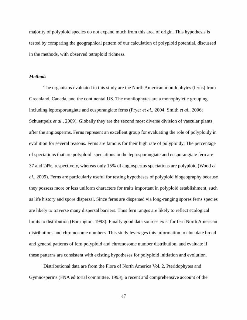
47
majority of polyploid species do not expand much from this area of origin. This hypothesis is
tested by comparing the geographical pattern of our calculation of polyploid potential, discussed
in the methods, with observed tetraploid richness.
Methods
The organisms evaluated in this study are the North American monilophytes (ferns) from
Greenland, Canada, and the continental US. The monilophytes are a monophyletic grouping
including leptosporangiate and eusporangiate ferns (Pryer et al., 2004; Smith et al., 2006;
Schuettpelz et al., 2009). Globally they are the second most diverse division of vascular plants
after the angiosperms. Ferns represent an excellent group for evaluating the role of polyploidy in
evolution for several reasons. Ferns are famous for their high rate of polyploidy; The percentage
of speciations that are polyploid speciations in the leptosporangiate and eusporangiate fern are
37 and 24%, respectively, whereas only 15% of angiosperms speciations are polyploid (Wood et
al., 2009). Ferns are particularly useful for testing hypotheses of polyploid biogeography because
they possess more or less uniform characters for traits important in polyploid establishment, such
as life history and spore dispersal. Since ferns are dispersed via long-ranging spores ferns species
are likely to traverse many dispersal barriers. Thus fern ranges are likely to reflect ecological
limits to distribution (Barrington, 1993). Finally good data sources exist for fern North American
distributions and chromosome numbers. This study leverages this information to elucidate broad
and general patterns of fern polyploid and chromosome number distribution, and evaluate if
these patterns are consistent with existing hypotheses for polyploid initiation and evolution.
Distributional data are from the Flora of North America Vol. 2, Pteridophytes and
Gymnosperms (FNA editorial committee, 1993), a recent and comprehensive account of the

48
continental North American ferns north of Mexico. This volume, henceforth FNA, has shaded
range maps for all 481 pteridophyte species, subspecies, and varieties. The ferns are a
monophyletic subset of the pteridophytes. Range maps in FNA were produced from herbaria
records by authors of each taxon treatment in the volume. For a full description of how these
shaded range maps were produced see the volume. From the FNA shaded range maps
geographical information system (GIS) polygon vector range maps were generated (by
Bogonovich) using ArcView 9.1 (ESRI, 2005). The chromosomal and ploidy level data came
from descriptions in the Flora of North America. We had distributional, chromosomal, and ploidy
level data for 309 fern taxa, encompassing most ferns in the study region. Status as allopolyploid
or autopolyploid was determined for 66 polyploids (52 allopolyploids, 14 autopolyploids).
All analyses were performed on a North American Lambert conformal conic projection
with standard parallels at 20°and 60°N latitude and the central meridian at 96°W. A gridded map
with 8732 50 X 50 km cells (2500 km2) was created over North America using Hawth's Analysis
Tools for ArcGIS (Beyer, 2004) and used as a base-map. All analyses were applied to this grid.
There is some distortion of area in Lambert conformal conic projections, but it is low in the
region of analysis (Bolstad, 2005) and is not expected to affect general results. Climate data
(mean annual temperature, MAT) were sourced from the Worldclim dataset (Hijmans, 2005;
http://worldclim.org/). A 2.5 minute resolution raster map of MAT was converted to a point
vector map. Using a spatial join, average MAT was calculated for each grid cell.
Using the above geographic and climate data, the chromosome number and ploidy level
for the North American fern flora was calculated for each 2500 km2
grid square. Genomic
variables for each species were associated with the appropriate GIS range map and overlaid onto
the gridded base map. Several floristic measurements were calculated for each 2500 km2
grid

49
square based on the set of species overlapping each square. These floristic measurements include
the chromosomal mean, median, species and polyploid richness variables, and polyploid species
percentages (Table 3.1). A glaciation variable was constructed in the following manner. Grid
cells were coded as being glaciated or not depending on whether they were within the limits of
the Wisconsin glacial maximum. Using these variables the association of latitude and
temperature with polyploidy and chromosome number was evaluated. The existence or non-
existence of a PLFG was determined.
A null model for polyploid species distribution was developed which we term polyploid
potential. Polyploid potential is based on the premise that polyploids form haphazardly where the
opportunities for formation exist, namely where potential parent species geographically overlap.
Thus where a greater number of potential parent species overlap, a greater number of polyploid
species should be found. Polyploid potential, takes into account all co-occurring species which
could putatively produce polyploid hybrid species. This metric is conceived on the premise that
only closely related species (congeners) may produce polyploids. The following equations were
used to calculate polyploid potential for each 2500 km2
grid square.
Equation 1. Polyploid potential excluding autopolyploids
∑i=1
n1
2xi
2−
1
2xi
Equation 2. Polyploid potential including autopolyploids
∑i=1
n1
2xi
2+
1
2x i
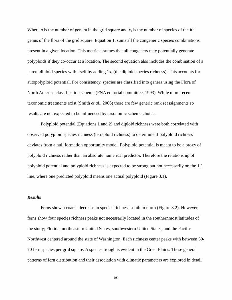
50
Where n is the number of genera in the grid square and xi is the number of species of the ith
genus of the flora of the grid square. Equation 1. sums all the congeneric species combinations
present in a given location. This metric assumes that all congeners may potentially generate
polyploids if they co-occur at a location. The second equation also includes the combination of a
parent diploid species with itself by adding 1xi (the diploid species richness). This accounts for
autopolyploid potential. For consistency, species are classified into genera using the Flora of
North America classification scheme (FNA editorial committee, 1993). While more recent
taxonomic treatments exist (Smith et al., 2006) there are few generic rank reassignments so
results are not expected to be influenced by taxonomic scheme choice.
Polyploid potential (Equations 1 and 2) and diploid richness were both correlated with
observed polyploid species richness (tetraploid richness) to determine if polyploid richness
deviates from a null formation opportunity model. Polyploid potential is meant to be a proxy of
polyploid richness rather than an absolute numerical predictor. Therefore the relationship of
polyploid potential and polyploid richness is expected to be strong but not necessarily on the 1:1
line, where one predicted polyploid means one actual polyploid (Figure 3.1).
Results
Ferns show a coarse decrease in species richness south to north (Figure 3.2). However,
ferns show four species richness peaks not necessarily located in the southernmost latitudes of
the study; Florida, northeastern United States, southwestern United States, and the Pacific
Northwest centered around the state of Washington. Each richness center peaks with between 50-
70 fern species per grid square. A species trough is evident in the Great Plains. These general
patterns of fern distribution and their association with climatic parameters are explored in detail

51
in Chapter 2.
130 species or 42% of North American ferns are polyploid (Figure 3.3). Most of the
polyploid species in our study are tetraploid but 26 species are triploid, three species are
pentaploid and four species are hexaploid. The overall pattern of polyploid richness is illustrated
in Figure 3.4. The peak in the southwestern U.S. is largely composed of triploid autopolyploids,
and these species contribute largely to the southwestern species richness peak observed in Figure
3.2.
Maps of percent tetraploids, mean chromosome number, and median chromosome
number are shown in Figures 3.4-3.6. Visual inspection of Figure 3.4 reveals there is no strong
association between percent tetraploids and latitude. Percent polyploidy does not strongly scale
with temperature or latitude (Figure 3.4, Table 3.2); neither does overall polyploid richness
(Table 3.2). We do not find that polyploid species are at higher relative frequency in formerly
glaciated regions than unglaciated regions (Table 3.2).
A strong positive chromosomal latitudinal pattern is evident in Figure 3.5. Median
chromosome number displays a similar geographical pattern (Figure 3.6). The geographical
pattern is not entirely explained by latitude. Coastal regions have lower average chromosome
numbers than interior regions at the same latitude. Interior regions, particularly in western North
America, have higher average chromosome numbers as compared to other regions of similar
latitude. These geographical patterns suggest a relationship between temperature and
chromosome number. Indeed chromosome number scales inversely with mean annual
temperature (MAT) and the correlation is high, 72% (Figure 3.7, Table 3.2). Median
chromosome number also scales inversely with temperature albeit the relationship is somewhat
weaker (r-squared = 0.62). This nonetheless strong relationship suggests that the pattern of

52
association between average chromosome number of a region and mean annual temperature is a
robust relationship and not solely a result of the influence of a few outlier taxa with high
chromosome numbers.
Polyploid potential equation 2 strongly correlates with with observed tetraploid richness
(Table 3.2, Figure 3.8). In Figure 3.8 each point represents a single 2500 km2
grid square.
Diploid richness also strongly correlates with tetraploid richness. Thus overall diploids and
tetraploids have similar geographical richness patterns. The slope of the regression of tetraploid
richness on polyploid potential is 0.130 and the intercept is close to zero. This means that within
each region (2500 km2
grid square) about 0.13 or ~1/8 of potential polyploids are actually
formed according to the congener relatedness criterion. In Figure 3.8, a majority of regions fall
along the regression line. However there are some locations approaching the 1:1 line. These
regions correspond to Florida and a small region in the southwestern U.S. Polyploid potential is a
slightly poorer predictor of tetraploid richness than diploid richness, presumably in part because
of this pattern.
Discussion
The expectation that polyploids are in greater frequency in northern, colder, and formerly
glaciated regions, was not confirmed in the overall geographical pattern of polyploids (Figure
3.4, Table 3.2). Instead a null model, based on extant opportunities for polyploid formation,
predicts observed polyploid geographical distribution (Figure 3.8, Table 3.2). The geographical
pattern of fern tetraploid richness is highly correlated with diploid richness (Table 3.2)
suggesting no systematic directional distributional evolutionary changes experienced by
polyploids compared to their diploid progenitors, either in their formation, or subsequent
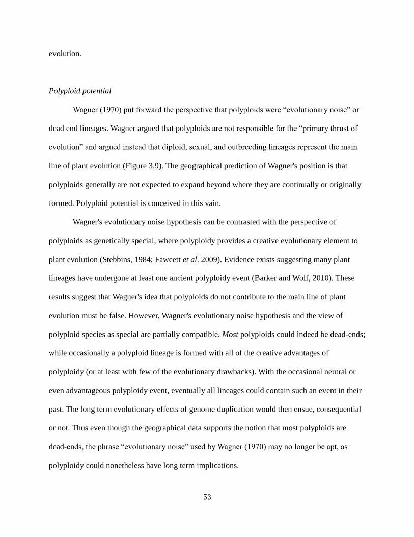
53
evolution.
Polyploid potential
Wagner (1970) put forward the perspective that polyploids were “evolutionary noise” or
dead end lineages. Wagner argued that polyploids are not responsible for the “primary thrust of
evolution” and argued instead that diploid, sexual, and outbreeding lineages represent the main
line of plant evolution (Figure 3.9). The geographical prediction of Wagner's position is that
polyploids generally are not expected to expand beyond where they are continually or originally
formed. Polyploid potential is conceived in this vain.
Wagner's evolutionary noise hypothesis can be contrasted with the perspective of
polyploids as genetically special, where polyploidy provides a creative evolutionary element to
plant evolution (Stebbins, 1984; Fawcett et al. 2009). Evidence exists suggesting many plant
lineages have undergone at least one ancient polyploidy event (Barker and Wolf, 2010). These
results suggest that Wagner's idea that polyploids do not contribute to the main line of plant
evolution must be false. However, Wagner's evolutionary noise hypothesis and the view of
polyploid species as special are partially compatible. Most polyploids could indeed be dead-ends;
while occasionally a polyploid lineage is formed with all of the creative advantages of
polyploidy (or at least with few of the evolutionary drawbacks). With the occasional neutral or
even advantageous polyploidy event, eventually all lineages could contain such an event in their
past. The long term evolutionary effects of genome duplication would then ensue, consequential
or not. Thus even though the geographical data supports the notion that most polyploids are
dead-ends, the phrase “evolutionary noise” used by Wagner (1970) may no longer be apt, as
polyploidy could nonetheless have long term implications.

54
Polyploid potential is designed to predict the overall whole flora patterns of polyploid
distribution. It is meant to predict the general patterns of polyploids, not outlier cases where a
polyploid event has initiated geographical expansion and evolution. The outliers may be of more
interest than the general pattern. The long term importance of polyploidy in evolution could be a
consequence of the few successful polyploids out of many dead-ends. The match between
polyploid potential and actual polyploid distribution simply highlights the difficulties faced by
new polyploid species.
We are presenting a perspective where polyploids are formed based on parent proximity
and opportunities for formation; and possibly most polyploids exist due to continual formation.
This perspective leads to predictions which could be explored in future research. One, many
extant polyploids may have multiple geneses. A single genesis requires the extant distribution of
a polyploid species to be the result of expansion and survival from the time and place of a single
founding event. A multiple geneses origin lacks this requirement and is more consistent with the
hypothesis that a polyploid species exists due to continual formation rather than a successful
establishment. The existence of polyploids with multiple geneses has been confirmed already. A
second prediction is that many extant polyploids should be young, because many of them are
maintained by continual formation. Current populations should trace their lineages to a formation
event in the recent past. Molecular clocks could give order of magnitude estimates on polyploid
species age. Three, experimental taxonomy techniques should show that of the congeners that
overlap geographically, the ones that most easily produce hybrid polyploids in the lab are the
ones that have done so in nature. Finally, where polyploid parentage is known, polyploids should
generally be confined either to the region of their parents geographical overlap, or at least be
confined to regions where one of their parents is present. To test this prediction polyploid and

55
parent species distributions should be mapped together, and regions of overlap evaluated. In
angiosperms, polyploid species tend to possess smaller ranges than diploid species (Martin and
Husband, 2009). This pattern is consistent with the preceding prediction because the region of
overlap of two diploid parental species should be the same size or smaller than the smallest range
of two parental species. Mapping polyploids and their parents together will provide a more
precise test of the prediction. Our results (in preparation) generally confirm the prediction that
polyploids are restricted to the area of parental species overlap.
For the calculation of polyploid potential, generic rank is used as a proxy for relatedness.
However, generic rank may be too strict or loose a criterion for the degree of relatedness
allowing hybrid polyploid formation. Genera, as they have been circumscribed by taxonomists,
probably vary in how much their constituent species are related both temporally and molecularly.
Additionally, there may be natural variation between taxa in how related their species must be to
produce polyploids. For these reasons polyploid potential was expected to be a proxy of
polyploid richness not an absolute numeric predictor; results matched these expectations, r-
squared between polyploid potential and tetraploid richness was high (0.62), but the slope of the
regression line was much lower than one (β = 0.130). There may be congeners within many
genera that are too distantly related to produce polyploids (even if they overlap geographically).
This would result in a relationship between polyploid potential and polyploid richness on a line
below the 1:1 line as found. Alternatively, a similar low slope may be expected if polyploid
formation is dependent on a degree of relatedness similar to what is found among congeners, but
the actual formation of polyploids is rare and stochastic such that only a percentage of the
potential polyploids will successfully form and establish. Future research will be needed to
resolve these issues.

56
Polyploidy potential (Equation 2) is based on extant distributions and extant opportunities
for polyploid formation. If a diploid parent species was present in a region and had since become
extirpated or its range shifted northward, perhaps following retreating glaciers, the daughter
polyploid species may still nonetheless be present in the region. Additionally, if the polyploid
daughter experienced directional selection and range expansion, it could expand beyond its
parent species range (if autopolyploid) or beyond the region where its parent species ranges
overlap (if allopolyploid). Either of these kinds of polyploid presences are not accounted for in
polyploid potential. However, there are several plausible reasons why polyploid potential
nonetheless successfully predicts tetraploid richness. First, if most current polyploids were
recently formed this would mean less time for obfuscating range shifts to occur. Second, taxa are
evolutionarily conservative in their environmental tolerances (Ricklefs and Latham, 1992; Qian
and Ricklefs, 2004a). Parent species ranges overlap presumably because their climatic
environmental tolerances overlap. The daughter polyploid species will inherit the additive
genetic variation for the climate environmental tolerances from this region of overlap. Therefore,
even if climate change occurs and species ranges shift in response, one can expect that
polyploids may follow its parents range overlap in climate condition niche space and hence
geographical space. There is evidence for long term stasis in the climate tolerances of lineages
despite shorter term climatic shifts (Ricklefs and Latham, 1992; Qian and Ricklefs, 2004a).
Finally, the observation that hybrids frequently occur where their parents are found at a local
level suggests an important role for proximity in polyploid formation. Theories have been
developed suggesting that initiated polyploids would have a minority cytotype disadvantage.
Perhaps, consistent with theory, many or most observed polyploids species are simply
continually formed in regions of parental overlap and infrequently expand beyond this, because

57
they fail to overcome minority cytotype disadvantage. Under this circumstance the overall
pattern of polyploid richness would match polyploid potential.
Chromosome geography
A very strong correlation (r-squared = 0.72) exists between mean chromosome number
and temperature. Earlier polyploid assignments were based on threshold chromosome numbers
as an indicator of polyploid status. Species above a certain threshold chromosome number were
deemed polyploids. Earlier authors may have misidentified the high chromosome numbers of
northern species as an indication of greater polyploid frequency in northern latitudes.
The latitudinal chromosome pattern may have implications for hypotheses on polyploid
distribution. If diploidization of polyploids proceeds at a rapid rate relative to any process that
generates polyploids at higher frequency in colder northern regions compared to warmer
southern regions, then a higher frequency of polyploid formation in higher latitudes could
countered by this rapid diploidization. Higher chromosome numbers would persist in higher
latitudes as a remnant of this long term higher rate of polyploidization. However, a higher rate of
polyploidy in northern latitudes could plausibly result from more neutral factors. In the lab cold
temperatures have been demonstrated to cause polyploid formation through induction of errors in
meiosis and mitosis. If this observation extrapolates to nature, then polyploid formation
frequency is increased by cold temperatures. The high average chromosome numbers in northern
latitudes could reflect influence of temperature on rate of polyploidization (again followed by
rapid diploidization).

58
Figures and Tables
Figure 3.1. Plotted are conceivable relationships between polyploid potential and tetraploid
richness, where polyploid potential of a region is on the x axis, with the number of tetraploids in
the region on the y axis. Data points would be individual regions, in this case 2500km2 grid
squares. If our criteria for polyploid formation are valid, namely that tetraploid species are only
formed by congeners and only by parents currently present where the tetraploid is present, then
we would expect no regions to have higher tetraploid richness than polyploid potential would
indicate, corresponding to the data region above the 1:1 line. Relationships that fall below the 1:1
line would suggest either that our congeneric formation criteria is too phylogenetically broad, or
that many potential polyploids fail to form despite the proximity of their potential parent species.

59
Figure 3.2. Monilophyte richness. Note how the distribution of richness is centered in at least
four peaks, one in the Southwest, Pacific Northwest (U.S.) and Southwestern Canada, Florida,
and the Northeastern U.S./Southeastern Canada, surrounding the Great Lakes region and
Northern Appalachians. The latter peak is the largest in geographical area.
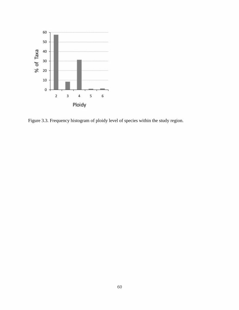
60
Figure 3.3. Frequency histogram of ploidy level of species within the study region.

61
Figure 3.4. Percent tetraploids. Note the poor relationship with latitude.

62
Figure 3.5. Mean chromosome number of species found in each map cell. Note the strong
relationship with latitude.

63
Figure 3.6. Median chromosome number of species found in each map cell. Note that the strong
relationship with latitude is similar to that pattern found in Figure 3.5.

64
Figure 3.7. Scatter plot of mean chromosome number on mean annual temperature. Points are
individual 2500km2 grid squares. R-squared is 0.72.

65
Figure 3.8. Scatter plot of tetraploid richness on polyploid potential (Equation 2). Plotted are
individual 2500km2 grid squares. Most locations fall on a general relationship where about 13%
of predicted polyploids are present. Some locations are outliers to this relationship with nearly as
many tetraploids as would be predicted by polyploid potential equation 2 (points close to the 1:1
line). Few locations possess more tetraploids than predicted by polyploid potential (absence of
locations above the 1:1 line). In other words, there are rarely more polyploids than would be

66
accounted for by polyploid potential equation 2. Locations that possess many fewer polyploids
than expected given the fitted relationship are noticeably absent (lower right region of scatter
plot). Positive outliers correspond to the American Southwest (Arizona) and Florida.
Figure 3.9. Polyploids as evolutionary noise. Reprinted from Wagner (1970), Figure 1. Original
text: Main lines represent normal, diploid, sexual, outbreeding species; broken lines indicate
polyploids, apomicts, and inbreeders; dots stand for hybrids.

67
Table 1: Summary of variables used in this study
Type Variable Source
Predictor Glaciation binary
'' Latitude degrees GIS
'' Mean annual temperature °C * 10
'' Polyploid potential species Equation 1.
'' Diploid richness species
Response Mean chromosome number chromosomes
'' Median chromosome number chromosomes FNA
'' Allopolyploid richness species
Autopolyploid richness species
'' Tetraploid richness species
'' Percent tetraploid % species
'' Percent polyploid % species
Units
Worldclim1
FNA2
1 (Hijmans et al. 2005) 2 (FNA editorial committee 1993)
Table 3.1. Variables in this study, calculated or collected for each map grid square.
Table 2: R-squared values
Latitude Mean annual temp. Polyploid potential Diploid richness
Tetraploid richness 0.02 0.24 0.62 0.71
% Tetraploid 0.01 0.07 0.01 0.01
% Polyploid 0.00 0.05 0.00 0.00
Mean chr. number 0.09 0.73 0.07 0.43
Median chr. number 0.08 0.66 0.11 0.48
Allo. richness 0.01 0.18 0.57 0.64
Auto. richness 0.06 0.33 0.04 0.25
Table 3.2. R-squared values. Predictor variables are in columns, response variables in rows. R-
squared values over 0.50 are in bold type.
68
Chapter 4. Using species elevation data and range maps to infer thermal niche range of North
American fern and lycophyte families
Abstract
This paper describes the methodology employed to create GIS species range maps for
North American ferns using two floras, the Flora of North America Vol. 2 (Continental United
States, Canada, and Greenland) and The Pteridophytes of Mexico (Mexico). GIS range maps are
constructed utilizing information from both floras, and both kinds of distribution information
contained within them - species geographical range and elevational range. First, using GIS
software species range map polygons are constructed. Then, with a digital elevation map (DEM;
a raster based map of elevation), areas within each species ranges that are either above or below
the reported elevational range of the species are excised from the species range maps. These new
range maps form the bases for many analyses in the following two chapters where they are used
to infer the thermal niches of fern taxa. These maps will be referred to as EX-NAM, EX for the
elevational excision, NAM for North America. The primary purpose of this chapter is to test if
thermal niche of fern taxa can be accurately estimated using these elevation adjusted maps. To
this end, minimum mean annual temperature (minMAT) of fern families is estimated from the
species range maps of the EX-NAM database and these estimates are compared with fern family
minMAT estimates two other fern distributional databases (NAM and GBIF). The first database
is the EX-NAM range maps prior to elevational excision (or simply NAM). The second database
is an herbarium record database constructed from the global biodiversity information facility
(GBIF). We ask if EX-NAM minMAT estimates are well correlated with GBIF minMAT
estimates. We find that the NAM estimates underestimate family minMAT in comparison to both
69
EX-NAM and GBIF estimates. EX-NAM and GBIF estimates are strongly correlated and similar
in magnitude. Since EX-NAM minMAT estimates are close to minMAT estimate derived from
and herbarium record database, we conclude that taxon thermal niche can be realistically
estimated using the elevational excision technique employed in the EX-NAM database.
Introduction
Plants are known to be distributed in highly predictable ways across elevational zones
(see Humboldt, 1805). Thus, in addition to species range data (e.g. shaded species range maps or
political unit presence maps) floras often report species elevational range data. Two floras
covering the ferns and lycophytes of North America contain both kinds of data. Flora of North
America (FNA) covers ferns from the regions of the continental United States, Canada, and
Greenland. The Pteridophytes of Mexico (POM) covers the Mexican ferns.
Species distributions are often reported as shaded species range map polygons as is the
case in FNA. In Chapter 2, GIS range maps were generated from the shaded range maps from
FNA. Alternatively, species range maps can be reported by presence in political units like
counties or states, such as is the case in POM. The latter system can be thought of as species
range map polygons, with species boundaries being confined to arbitrary political units. FNA and
POM data are ultimately based on specimen records, but this raw information is lost in the
reported species distribution summaries.
Species range maps present a species as present everywhere within the polygon, when in
reality there are often large regions within a species range polygon where individuals are not
present. These false positives or errors of commission can lead to substantial differences in the
estimation of species distribution or species richness between databases using species range

70
maps vs. databases based directly on specimen records (Hurlbert and White, 2005). Hurlbert and
White (2005) discovered that estimate differences between specimen record databases and range
map databases of North American birds were particularly pronounced in regions with elevational
variation. Of interest here, these errors of commission are also likely to influence estimates made
of species or family thermal niche parameters from such distribution databases.
When species elevational range data are available, regions above and below the
elevational range of a species can be excised from the species range maps, thus potentially
mitigating the false positive problem inherent in the use of raw species range maps. This type of
fine tuning should be particularly useful when examining parameters like thermal niche. This
excision technique is employed on the the combined range maps from FNA and POM, and the
resulting maps will be called the post-excision NAM database, or EX-NAM. The pre-excision
database will be referred to as NAM (combined range maps of FNA and POM prior to an
elevational excision).
The purpose of this study is to determine if maps with elevational excisions (EX-NAM
maps) can be used to generate reasonable estimates of the thermal niche of fern families. To
determine if this is likely to be true, I perform several analyses. First I ask if particular
elevational zones within Mexican states have low variation in MAT compared to Mexico's
thermal range as a whole. If true, this would mean that knowledge of the presence of a particular
species in such a state-elevation region gives a good idea of the MAT conditions under which
that species is persisting, relative to the total range of MAT variation within Mexico. Next, I ask
whether a fern family's minMAT (the minimum MAT within a family's range) is similar if
estimated by the EX-NAM database versus a specimen record database (GBIF database, Global
Biodiversity Information Facility). If estimates are similar, this would demonstrate that the

71
elevational excision technique effectively mitigates problems associated with errors of
commission inherent in species range map data, as identified by Hurlbert and White (2005).
Finally, I ask if fern family minMAT estimates made using the EX-NAM versus NAM databases
are similar or if NAM tends to underestimate minMAT relative to EX-NAM. The latter would be
expected if simple range maps tended to mark species as present in regions where they were not,
such as on mountaintops.
Broadly, results show that the elevational excision technique mitigates the problems with
species range maps identified by Hurlbert and White (2005). Estimates of fern family thermal
niche made using the EX-NAM database are comparable to estimates derived from the GBIF
herbaria record database, while the pre-excision database (NAM) consistently generates colder
estimates for fern family minMAT. These results suggest that the elevational excision technique
will allow floristic elevational and range map data to be combined to make decent estimates of
taxa thermal niche parameters.
Methods
Species range map generation
FNA species descriptions provide shaded species range maps, while POM reports species
presences in Mexican states. Both floras require at least one herbarium record in a state/province
(U.S., Canadian, or Mexican) to mark a species as present in that state/province, or (for FNA) to
shade in some portion of that state/province. FNA species range maps are not constrained by
political polygons. For example a species that exists only in southern Ontario could be drawn as
such. Additionally, FNA and POM report elevational range data for their respective regions for
each species. For a full description of species distribution data, reference the volumes.

72
Initial GIS species range maps were generated from FNA (see Chapter 2) and POM, and
these range maps were merged and now will be referred to as the NAM distribution database.
Then using a DEM (digital elevation map, 2.5 arcminute resolution) regions were excised from
NAM species range polygons that were either above or below that species elevational range.
Elevation ranges were available for FNA and POM separately so for species straddling the US-
Mexican border elevational excisions were applied to those regions separately. So for example,
Astrolepis integerrima is reported as present in the state of Coahuila, Mexico (Figure 4.1). The
elevational range in Mexico for A. integerrima is 800-2600m. Regions in Coahuila which are not
within that range of elevation are excised from that species range polygon for that state. Figure
4.1 illustrates the resulting EX-NAM species range map polygon. The range maps are complex,
often with both non-contiguous regions and lacunae (holes). To generate the EX-NAM database,
elevational ranges are rounded to the nearest 100 meters.
The regions that are removed using the elevational excision technique are often
geographically small (such as the top of a mountain) but are often environmentally (and
thermally) different from surrounding regions. When determining thermal niche range
parameters for a species, for example, the erroneous inclusion of unoccupied mountaintops in the
species range would lead to underestimates of the minimum mean annual temperature within the
species range (species minMAT).
Mexican species ranges are reported in POM by their presence or absence in Mexican
states. Recall, to construct the EX-NAM range maps, elevations throughout North America are
rounded into 100m bins. Therefore, within Mexico, in EX-NAM range maps, species are
reported as present or absent within a finite number of state-elevation operational geographical
units (state-elevation OGUs). For example, there is a region in the state of Veracruz between 0-

73
100 meters elevation in which all Mexican species are either determined as present or absent.
Species range maps with elevational excisions generated from FNA are merged with their
corresponding range map in Mexico (POM) when the species exists in both regions. The entire
study region contains 1339 fern and lycophyte species, with 1033 in Mexico and 481 in North
America north of Mexico. The resulting database is referred to as the EX-NAM distribution
database.
Analyses
Temperature range within Mexican state-elevation OGUs
The question I address here is the following. What is the range of mean annual
temperatures (MAT) found within Mexican state-elevation OGUs? A Mexican state-elevation
range would be regions between certain elevations within a single Mexican state (e.g. 0-100m in
Veracruz). If the range of MAT values within most or all state-elevation OGUs is small in
comparison to the total range in variation of MAT across Mexico then a distribution database
based on such OGUs can be used to estimate the thermal niche (MAT niche) of a species within
Mexico. However, if the range of MAT values within the state-elevation OGUs is frequently high
then estimating the thermal niche of a species based on species state-elevation OGU presences
would lead to substantial error. For example, a species might be recorded in a particular state-
elevation OGU, but may only persist in regions of that OGU that have high MAT. The species
plausibly would not persist in other regions of the OGU that have lower MAT. However, because
the range map is based on state-elevation OGU presence/absence, the species range map would
incorporate these regions of low MAT. Thus, in this case, the minimum MAT of the species will
be substantially underestimated.

74
The range of MATs within Mexican state-elevation OGUs was determined using MAT
data from the Worldclim dataset (Hijmans, 2005). Twenty sample points were generated within
each OGU and the MAT values of these points were determined by overlaying them on the
Worldclim MAT map with a resolution of 2.5 arcminutes (an arcminute is ~4.65 km). OGU MAT
ranges (plotted in Figure 4.2) were obtained from the sample points.
EX-NAM vs. GBIF database comparison
I compare fern family minMAT as estimated using the EX-NAM database to minMAT as
estimated using the GBIF database (Global Biodiversity Information Facility), a database of
specimen records with precise coordinates.
The EX-NAM range maps are still polygons and so the concern remains that a species
will be represented in a region in which that species is not actually present. This could lead to
errors in estimation of a species (and family's) thermal range. This error might be large even after
the employment of the elevational region excision technique described earlier. This EX-NAM vs.
GBIF comparison is meant to test if estimates of thermal niche derived from the EX-NAM
database are distorted. If the EX-NAM and GBIF databases yield similar estimates of minMAT
we can conclude that the EX-NAM database is roughly as effective as herbaria records for
estimating minMAT and thermal niche.
Using the EX-NAM distributional database, family ranges are generated by merging the
species range map polygons of all species in the family. For each family minMAT was
determined by overlaying the family range on the Worldclim MAT map. GBIF data were used to
estimate fern family minMAT in the following manner. 99,316 fern electronic specimen records
were accessed on October 2nd
2010 from GBIF (http://www.gbif.org). Records were classified by

75
family and the minMAT for each family was determined by overlaying the points onto the
Worldclim MAT map. The two sets of estimates are regressed onto each other, and presented in a
scatter plot (Figure 4.3).
NAM vs. GBIF database comparison
Estimates of fern family minMAT were also generated from the pre-excision NAM
database. These estimates were generated in a similar manner with the Worldclim MAT map, and
were then correlated with the GBIF estimates.
Results
Temperature range within Mexican state-elevation OGUs
MAT values in Mexico range over 27.1 degrees Celsius. There are 935 state-elevation
OGUs in Mexico, only 19 (or 2%) contain a range of MAT values greater than 20% of the total
MAT range of 27.1 degrees in Mexico (Figure 4.2). The state-elevation OGU with the highest
range of MAT values, has an MAT range of 7.9 degrees, only 29% of the total (Puebla 1100-
1199m).
Correlations between thermal niche estimates based on fern distributional databases
EX-NAM and GBIF estimates for family minMAT are strongly correlated and close to
the 1:1 line (Figure 4.3; r-squared = 0.8763; Lycopodiaceae excluded). Lycopodiaceae is an
outlier with the GBIF minMAT estimate for that family being much warmer than the EX-NAM
estimate. Lycopodiaceae is excluded from remaining plots.
Estimates of fern family minMAT made from the pre-excision NAM database do

76
correlate with GBIF estimates (Figure 4.4). However, the r-squared is slightly lower than the r-
squared for EX-NAM and GBIF (0.825 vs. 0.8763). More importantly, EX-NAM fern family
minMAT estimates tend to be lower than GBIF estimates. This is reflected in Figure 4.4, by the
fact that the relationship is positioned to the left of the 1:1 line.
Finally, EX-NAM and NAM fern family minMAT estimates are correlated, but the NAM
estimates tend to be lower than EX-NAM estimates (Figure 4.5). Again, this is reflected by the
fact that the relationship is positioned the left of the 1:1 line.
Discussion
The assessment tests performed indicate that the fern distributional dataset using an
elevational excision technique can be used to assess thermal niche ranges of fern families,
genera, and species. The first test demonstrates that Mexican state-elevation OGUs do not
contain a wide range of MAT values within their boundaries in comparison to the full range of
MAT within Mexico. Thus, knowledge that a species exists within a state-elevation OGU gives a
reasonably accurate description of MAT conditions that that species tolerates. The comparison
tests show that the thermal niche estimates based on the EX-NAM database are comparable to
estimates based on a raw specimen record database (Figure 4.3). This result suggests that EX-
NAM range maps (range maps with elevational excisions) do not cause distortions of niche
parameter estimation such as one would expect with typical range maps. Next, estimates made
from the NAM prior to elevational excision tend to underestimate fern family minMAT relative
to EX-NAM estimates. This is the result that would be expected if NAM range maps erroneously
included regions with low MAT (such as mountaintops).
The EX-NAM database is constructed from distribution summaries (shaded species range

77
maps, state presence/absence, and elevation ranges) found in the original volumes, FNA and
POM. However, these summaries are ultimately based on specimen records, many of which are
probably identical to the set of GBIF specimen records (this raw specimen information is lost in
the FNA and POM distribution summarizations). Potentially, FNA, POM, EX-NAM (based on
FNA and POM), and GBIF might represent similarly incomplete estimates. To allay this concern,
one can point to studies of botanical exploration. Soria-Auza and Kessler (2008) retrospectively
examined the accumulation of specimen records of ferns in Bolivia. They show that the pattern
of species diversity was determined early on in the process of exploration. North America is
comparatively less diverse and probably better sampled providing confidence that distribution
estimates of species (and especially families) probably reflect genuine distribution patterns.
If the GBIF and EX-NAM databases yield similar estimates of thermal niche, then why
generate and use the EX-NAM estimates? While GBIF has the potential to eventually become
the system for storing global biodiversity knowledge, currently the GBIF database is still
relatively incomplete (Guralnick et al., 2007; Yesson et al., 2007); at the time of writing, the
GBIF database did not have enough specimen records to make fine taxonomic scale estimates as
the EX-NAM. Therefore, the EX-NAM database is used throughout the remaining chapters.

78
Figures
Figure 4.1. Range map of Astrolepis integerrima (dark grey region on map). This is a typical
range map within the EX-NAM fern distributional database. Data north of the Mexico-United
States boundary, derive from FNA. Data south of the Mexico-United States boundary derive
from POM. Each volume, FNA and POM report elevation range data for each species for their
respective regions. The black dotted line represents the outline of the species range map polygon
for A. integerrima north of Mexico. Regions either above or below the reported elevational range
of A. integerrima are excised from this species range map polygon and the result is the complex
elevational regions visible within the black dotted line. South of the Mexico-United States
boundary, the reported elevational range of the species in Mexico is used in a similar way, except
that species range polygons in Mexico correspond to the set of states in which the species is
reported as present.

79
Figure 4.2. Plot of thermal range within Mexican state-elevation OGUs (operational
geographical units). OGUs are ordered from left to right by the minimum MAT found within
their boundaries. Note that each OGU has a range of MAT values much less than the full range of
MAT values over the whole region of Mexico (degrees Celsius).

80
Figure 4.3. Scatter plot of North American of fern family thermal niche minimum (minMAT,
minimum mean annual temperature within family range) as estimated by two different datasets,
EX-NAM and GBIF (see text). The GBIF minMAT estimate in on the y-axis, and the EX-NAM
minMAT estimate is on the x-axis. Note the strong relationship, close to the 1:1 line.

81
Figure 4.4. Scatter plot of North American of fern family thermal niche minimum (minMAT,
minimum mean annual temperature within family range) as estimated by two different datasets,
the pre-excision NAM database and the GBIF database (see text). The GBIF minMAT estimate is
on the y-axis, the NAM minMAT estimate is on the x-axis. Note that the relationship is
positioned left of the 1:1 line.

82
Figure 4.5. Scatter plot of North American of fern family thermal niche minimum (minMAT,
minimum mean annual temperature within family range) as estimated by two different datasets,
the pre-excision NAM and post-excision EX-NAM database (see text). The EX-NAM minMAT
estimate is on the y-axis, the NAM minMAT estimate is on the x-axis. Note that the relationship
is positioned left of the 1:1 line.

83
Chapter 5. The Russian doll pattern: A test of the Out of the Tropics (OTT) hypothesis with
North American ferns
Abstract
The distribution patterns of extant North American ferns and lycophytes are evaluated for
consistency with the out of the tropics (OTT) hypothesis. The OTT hypothesis describes one
possible scenario for the evolutionary and geographical dynamics underlying the latitudinal
diversity gradient (LDG). The OTT hypothesis has been evaluated chiefly for marine higher
taxa; here I extend the analysis to a terrestrial group, the speciose North American ferns and
lycophytes. The OTT proposes that higher taxa more frequently originate in the tropics than the
extra-tropics and that some of these lineages then expand into temperate and polar regions while
maintaining their presence in the tropics. Jablonski et al. (2006) outlined consistency tests of the
OTT hypothesis. Predictions include the following. (1) Taxa confined to the tropics (endemic to
the tropics) will be more common than taxa confined to the extra-tropics. (2) The average age of
extra-tropical higher taxa will be older than tropical higher taxa because it takes time for taxa to
expand from their tropical place of origin. (3) Taxon richness (the number of species in a taxon)
should predict how far north a taxon extends. These predictions are evaluated using fern family
distribution data from two taxonomic treatments of North American ferns together with a recent
fossil constrained dated phylogeny. Higher taxa are individual fern families. Latitude and
minimum mean annual temperature within family geographical range (minMAT) are used as
tropical/extra-tropical variables. We find exceptionally strong support for two of the predictions.
The number of species in a fern family predicts its northern extension and minMAT. Secondly,
endemism is high in the tropics; family ranges display a nearly perfect pattern of nestedness

84
centered on the tropics, meaning endemic families are only found in the tropics, never in the
extra-tropics. However, contrary to expectations, families that extend into temperate and polar
regions are not, on average, older than families that are confined to the tropics. Alternative
explanations for observed patterns are considered (tropical conservatism hypothesis, TCH). In
summary the distribution of ferns partially conforms to the predictions of the OTT model.
However, direct tests of the OTT model are needed.
Introduction
A major feature of the geography of life on Earth is the latitudinal gradient in taxon and
species richness, with lower latitudes containing greater numbers of taxa. This pattern is referred
to as the latitudinal diversity gradient (LDG). Three parameters control the number of species in
a region: rates of origination, extinction and immigration (Equations 1 and 2, with figures below;
Jablonski, 1993). Asymmetries in these parameters along the latitudinal gradient could produce
the LDG; various combinations of these parameters have been proposed to account for the LDG.
For example Wallace (1878) proposed that the high biological diversity of the tropics resulted
from higher origination rates in the tropics than temperate and polar regions.
More recently Jablonski (1993) proposed that in addition to higher rates of origination in
the tropics, migration was also an important factor in generating the LDG. Jablonski's model is
called the out of the tropics (OTT) hypothesis, and essentially represents one concept about the
relative contributions of origination, extinction, and migration/expansion to the LDG. First, the
OTT model states that higher taxa more frequently originate in the tropics than the extra-tropics.
Second, these lineages expand over time into temperate and then polar regions while retaining
their presences in the tropics. Since many tropical taxa have only recently originated and, hence,

85
have not yet expanded into the extra-tropics, the OTT model predicts that younger higher taxa
should be found mostly in the tropics and only older taxa should be found in the extra-tropics.
The differences between tropics and extra-tropics in these two parameters alone, origination and
migration (without extinction) are thought to suffice to generate the LDG. Results from recent
papers are consistent with the OTT model's premise that origination rates (or rates of
diversification) are higher in the tropics (birds and butterflies, Cardillo, 1999; birds, Cardillo et
al., 2005; ocean plankton, Allen et al., 2006; plants, Eo et al., 2008).
The OTT model also predicts that more speciose higher taxa are expected to have
extended father north and into colder regions. Lineages that accumulate more species are
consequently expected to have more opportunities for dispersal and adaptive mutations allowing
one of these constituent species to expand into northern and colder regions. Additionally, older
higher taxa have had more time to accumulate species and will be expected to have expanded
further into the tropics.
To date the OTT model has been tested largely with shelled marine organisms that have
detailed fossil records (Jablonski et al. 2006; see Martin et al. 2007). Ideally, the OTT hypothesis
can be tested, relatively directly, by assessing the origination, migration and extinction rates in
the tropics and extra-tropics by examining lineage appearance and disappearance dates in the
fossil record. Jablonski et al. (2006), recognizing that not all lineages are as well characterized in
the fossil record as shelled marine organisms, outlined several consistency tests for the OTT
hypothesis to be used when detailed lineage origination and extinction times and location data
were not available. Instead, these consistency tests require extant distribution data and taxon ages
which can be derived from a dated phylogeny.
I test the OTT model on North American fern and lycophyte families. Ferns and

86
lycophytes disperse widely, so their distributions are likely strongly affected by climate and
constraints on evolutionary potential rather than dispersal barriers (Barrington, 1993). Therefore,
a cold thermal limit for a fern or lycophyte lineage likely reflects the coldest temperature in
which that lineage can persist not just the coldest temperature in which that lineages does persist.
Latitudinal gradients in fern and lycophyte richness have been found globally (Kreft et al., 2010)
and in the continental United States, Canada, and Greenland (Chapter 2) making ferns and
lycophytes appropriate taxa for the testing of the OTT model. My study region provides a good
stage against which to evaluate fern and lycophyte evolution because it encompasses climates
ranging from polar to tropical. Regions in Mexico, particularly southern Mexico, incorporate a
wide variety of tropical climatic conditions. Mexico contains 1033 fern and lycophyte species,
while North America north of Mexico contains 481 species. The entire study region contains
1339 of the roughly 12,000 – 15,000 fern and lycophyte species worldwide (worldwide estimate
by Roos, 1996). Thus, the study flora represents a substantial fraction of total global fern
diversity (~10%).
I investigate three predictions of the OTT model: (1) the tropics have a higher number of
endemic taxa than the extra-tropics (2) more speciose taxa extend farther north and farther into
colder regions (3) taxa that have extended to northern and colder regions are on average older
than taxa that have not expanded northward.
The following data were collected, fern family age, fern family latitudinal distribution
(latitudinal maximum and minimum), and minimum and maximum mean annual temperature
within family range (minMAT, maxMAT). (see Chapter 4 for a detailed description of the
distributional database and thermal niche ranges). Fern family ages (time since origination) were
determined using a recent fossil constrained and dated fern phylogeny (Schuettpelz and Pryer,

87
2009).
Results consistent with predictions confirm the OTT as a possible explanation for the fern
and lycophyte LDG. However, alternative explanations (various combinations of origination,
extinction, and migration rates) are still possible; these are explored in the discussion. Particular
attention is paid to the tropical conservatism hypothesis (TCH). Results leave explanations open,
but strongly curtail the set of possible and parsimonious explanations.
Methods
A fern family richness map was constructed by first combining the species range maps of
each family as detailed in Chapter 4. Then family range maps were overlaid onto a grid of 10,039
2500km2 grid squares (50 by 50km) covering North America and family richness in each cell
was tabulated by counting the number of overlapping family range maps (Figure 5.1).
OTT Consistency tests
Three predictions of the OTT model are tested. The prediction that the tropics should
have a higher number of endemic higher taxa is tested by plotting family latitudinal and mean
annual temperature (MAT) ranges in which high temperatures and low latitudes correspond to
the tropics (Figures 5.2 and 5.3). In this context, the term endemic families, refers to those that
are present in only the tropics or extra-tropics, but not both. A family that is endemic to the
tropics would be present only in low latitudes and high temperatures, and not in high latitudes
and low temperatures. To test whether more speciose taxa range farther north and into colder
regions I plotted fern families by their minMAT on their taxon richness, i.e., the number of
species in the family (Figure 5.4). I also test if peak richness of a family (the highest richness

88
observed in one location within the study region) predicts family northern range limit or
minMAT. Finally, to test the third prediction, that northern and colder regions will on average
possess older families, fern families were plotted by their minMAT on their age (Figure 5.5).
Fern family geographical distribution
Fern family range maps were obtained from the EX-NAM distribution database described
in Chapter 4. Family range maps were generated by merging all species range maps of the
family. Climate data were from a MAT map with a resolution of 2.5 arcminutes (~4.65 km) from
the Worldclim database (Hijmans et al., 2005). Thermal niche data for each fern family
(minMAT, maxMAT) was determined by overlaying each fern family on an MAT map
(converted from a raster MAT map to a vector point MAT map) and selecting the minimum and
maximum MAT values contained within the family range (minMAT, maxMAT). See Chapter 4
for a detailed description of the generation and evaluation of maps and taxon thermal niche range
inferred from these maps.
Latitude vs. MAT
We analyze patterns of family distributions primarily with respect to their MAT niche (the
range of mean annual temperatures of the regions in which families persist) rather than latitude.
Latitude is a spatial variable. Latitude can be thought of more as a proxy of factors such as MAT
and less of a variable of interest in itself (Hawkins, 2004).
Focusing on latitudinal range alone can be misleading. High mountains in tropical regions
often have very low temperatures and ecologies comparable to regions that are typically found
much farther north while northern regions tend not to possess the obverse, small patches of

89
tropical conditions. Temperate families might be expected to persist in high elevation regions in
tropical latitudes, while families suited for tropical conditions would not be expected much
farther north. This scenario would lead to a pattern where many or most lineages exist at low
latitudes (including climatically temperate families), but few climatically tropical families exist
farther north. Tropical regions would possess latitudinally endemic families, while northern
colder regions would not possess latitudinally endemic families, even though extra-tropical
regions would possess thermally endemic families. Thus, families that are thermally endemic,
could have originated in extra-tropical regions (inconsistent with the OTT model) and are merely
in the tropics because there are temperate conditions in tropical areas. This pattern would
spuriously appear consistent with an OTT model. Examination of the temperature ranges of
families allows an assessment of whether or not a family is genuinely present in tropical thermal
conditions, or simply at high elevation in low latitudes.
Taxonomy and fern family age
Fern family ages were determined from a recent fern phylogeny constructed by
Schuettpelz and Pryer (2009) that is dated with fossil constraints. Fern family ages were
determined by reading the age of the node sub-tending the species of the family. Family ages
were also determined from a fern phylogeny prepared by Michale Barker (in preparation).
Family age estimates determined from the two phylogenies are very similar (r-squared = 0.8593).
For generating family range maps the Smith et al. (2006) taxonomic scheme was employed.
Family level fern taxonomy has remained relatively stable for some time.

90
Ferns and Lycophytes
OTT tests were conducted on ferns (Division Polypodiophyta). Lycophytes (Division
Lycopodiophyta) were included in all but one test. Family age data were not available for
lycophytes from the Schuettpelz and Pryer (2009) phylogeny; thus, tests involving family age
data did not include lycophytes. For all other tests, results were similar whether lycophytes were
included or excluded.
Results
Ferns display a latitudinal diversity gradient (LDG) in North America (Figure 5.1).
Highest family richness values are found in Chiapas and Oaxaca, Mexico and richness decreases
to the north. The correlation between latitude and fern family richness is high (r-squared =
0.5796). A plot of the latitudinal ranges of individual families, demonstrates that ferns display a
strong LDG at the family level (Figure 5.2). Thirty-five families exist at the lowest latitude of the
study, and the number of families present diminishes moving northward.
Latitude/MAT and endemism
North American fern and lycophyte families have a strong latitudinal pattern of
endemism; lower latitude regions, and regions with higher MAT possess a greater number of
endemic families (Figures 5.2 and 5.3). There are families present in tropical latitudes or
temperatures but not present in extra-tropical latitudes and temperatures; however, the reverse is
not true. The pattern of endemism is nearly perfect; all endemic families are thermally and
latitudinally tropical. The extra-tropics are not only less diverse than the tropics, but represent a
near perfect subset of tropical lineages. The single exception is the Marsiliaceae, a monospecific

91
family that is not present at the lowest latitude of the study. Interestingly this exception is not
apparent in the temperature distributions. Otherwise, each family range in latitude or MAT
extends to the lowest latitude of the study or (roughly) the highest temperatures; the resulting
pattern observable in Figures 5.2 and 5.3 resembles a Russian doll, with smaller family ranges
nested within larger ranges.
Age vs. northern extension (range latitudinal maximum or thermal minimum)
Older fern families do not tend to extend into colder regions than younger families
(Figure 5.5). Instead, the regression illustrated in Figure 5.5 illustrates a very weak positive
relationship between family age and family minMAT (r-squared = 0.0225). So, in contrast to
expectations, older families are not more likely than younger families to extend into colder and
more northern regions.
Taxon richness and northern extension (MAT)
There was a strong relationship between taxon richness (the number of species in a
family) and the minimum MAT within a family range (all families, r-squared = 0.5403; families
with temperate richness peak, r-squared = 0.5162; families with tropical richness peak, r-squared
= 0.6463; Figure 5.4). More diversified families extend into colder regions. Interestingly, several
families do not have peak richness in the tropics even though all families are present in the
tropics (maps and figures not shown). Regardless, the region of peak richness for most families is
below 25 degrees latitude. The correlation between peak richness (usually in the tropics) and
northern extension (minMAT) is, r-squared = 0.4154. The correlation between peak richness and
northern minMAT for families with temperate peaks is, r-squared = 0.6385; for families with

92
tropical peaks, r-squared = 0.5730.
The order Polypodiales, the largest order of fern families, contains 14 fern families in the
study region. A regression between family taxon richness and minMAT, using families from this
order alone, yields a strong relationship, r-squared = 0.6161 (figure not shown).
Discussion
Results were partially consistent with OTT predictions. Family taxon richness predicts
family minMAT and maximum latitude, and the tropics contain more (all) endemic families than
the extra-tropics. One prediction is not supported. There is not a positive association between
family age and northern or thermal extension. Other processes described by the OTT model can
operate even if there is not a relationship between age and extra-tropical extension. If families
evolved to novel thermal conditions at very different rates, an age and extra-tropical extension
correlation might not be observed. Families that expand, but later retract would destroy a
correlation between age and expansion into the tropics.
In this study the OTT model is tested along a thermal gradient in addition to a latitudinal
gradient. This analysis demonstrates that patterns consistent with the OTT model aren't simple
artifacts of the spatial and elevational arrangement of thermal conditions. To understand why,
consider the following argument. The latitudinal Russian doll pattern, the pattern of near
complete nestedness of families centered on the tropics, could plausibly result from thermally
temperate families present in the tropics in colder, higher elevations. However, a Russian doll
pattern is visible in the thermal ranges of fern families as well, suggesting that the pattern of
endemism is not an artifact of the spatial arrangement of climatic conditions (temperate
conditions present in tropical latitudes without the obverse).

93
One apparent difference between Figures 5.2 and 5.3 is notable. All fern families (except
the Marsiliaceae) are present at the lowest latitude. On the other hand, the temperature (MAT)
containing the most fern families is not precisely the warmest temperature of the continent, but
around 18-19 degrees Celsius. Many families are not present in colder temperatures. Several
families are also not present in warmer temperatures; families appear to be filtered out moving
away from the 'optimal' mean annual temperature of 18-19 degrees Celsius. These thermal
distribution patterns may suggest that the region of greatest origination is at an optimal
temperature at around 18-19 degrees Celsius, and then over time higher taxa evolve and expand,
though at different rates, from this optimal origination temperature in both thermal directions.
Consistent with this interpretation, most of the families that have not expanded into the warmest
temperatures of the continent (MAT nearly 30 degrees Celsius), are also the families that have
undergone the least expansion into colder temperatures (i.e. endemic families on the right side of
Figure 5.3). Adaptive geographical evolution would be required to expand in any direction along
the thermal niche axis, from the center of origin.
Alternative explanations
Alternative processes could generate the observed distributional patterns (Figure 5.6).
Figure 5.6 illustrates the OTT process (Figure 5.6a), and three alternative underlying processes
(Figures 5.6b-5.6d). The Russian doll pattern (family range nestedness pattern) and the
association between tropical richness and northern/thermal extension constrains potential
underlying processes.
Figure 5.6b illustrates a scenario where origination is just as frequent at any latitude.
However, to generate a Russian doll pattern, any origination occurring in the extra-tropics would

94
need to be followed by a rapid expansion of that family southward. Otherwise, if this expansion
did not always occur, or took a very long time, some families would appear endemic in the extra-
tropics (contrary to what is observed). Additionally this migration/expansion southward would
need to be accompanied by an accumulation of species in the tropical distribution of that family
that matched the degree of northern extension of that family (not necessarily the same as the
latitude of origin). Figure 5.6b illustrates a possible (though apparently not plausible) process
underlying observed patterns. Figure 5.6c illustrates a process that is perhaps more plausible than
the process illustrated in Figure 5.6b. Still, the latitudinal depth of extirpations (how far south
extirpations extend latitudinally) would need to be proportional to the number of species in a
family.
The process illustrated in Figure 5.6d is perhaps the most plausible alternative to the OTT
process. Here, only two things need to occur. First, periodically, or recently, all lineages would
need to become extirpated in the extra-tropics. Second the re-expansion of lineages into colder
temperatures, would need to be proportional to the number of species in a family in its tropical
regions. Glaciers obviously cause a temporary extirpation in northern latitudes. However,
glaciers misleadingly resemble the required extirpation pattern. Glacial extirpations are spatial,
and do not necessarily remove species entirely but instead temporarily shift their ranges south.
Many species will simply track the climates to which they are suited and return to northern
regions when glaciers retreat. Indeed, many species ranges appear to be shifting to current
climate changes occurring over a very short time. Ferns, given their high level of dispersal
(Barrington, 1993), are especially likely to simply follow their required climatic conditions as the
move up and down the continent. Species ranges, when viewed in climate space (thermal niche
space), are more stable in comparison to the movement of species ranges in geographical space.

95
This has been referred to as phylogenetic niche conservatism in the literature (Wiens and
Donoghue, 2004; Wiens and Graham, 2005).
Counter-intuitively ancient global climate warming is more likely to produce the process
illustrated in Figure 5.6d than glaciation and associated global cooling events. A global warming
could remove all northern climates, and species adapted to that niche would become extinct (A
global cooling would not remove such climates from the globe). After a warming event, when
northern cool climates return, populations of families would have to newly adapt to such
conditions since their temperate representatives would have earlier gone extinct. Species in
families would adaptively evolve to colder climates to different degrees and at different rates.
This would lead to the observed Russian doll pattern. Families would still need to expand into
cool climates in proportion to their species richness in the tropics to be consistent with observed
patterns.
The tropical conservatism hypothesis (TCH; Wiens and Donoghue, 2004), essentially
outlines the above scenario. TCH suggests contrary to OTT, that history or the recent extirpation
of lineages in northern thermal conditions would play a major role in observed distribution.
Consistent with the TCH a global warming event occurred relatively recently, in the Eocene, 30-
40 mya (Behrensmeyer et al., 1992). According to the TCH, and contrary to the OTT, temperate
and tropical regions do not need to differ in diversification or taxon origination rate to produce a
LDG. According to the TCH, higher taxa merely have not had enough time to expand into and
diversify within temperate regions because these climates have been available for much less
time.
Results presented in this paper are consistent with both OTT and TCH. Nonetheless, I
believe the TCH is not likely to be the best explanation for the LDG. Global warming would
96
result in the disappearance of large areas of cold condition regions. However, some cold regions
would remain. Cool habitats associated with higher elevations would remain, enough for many
families to persist during warm periods. We will see in the following chapter that taxon richness
also predicts elevational extension.
Ultimately more information will be required to distinguish between the TCH and the
OTT model. If temperate lineages of many fern families are shown to be older than 30 or 40
million years, this could falsify the TCH. If most temperate lineages of fern families are more
recent then this would be strong support for the TCH. Regardless, the number of species in a fern
family is strongly correlated with its extension into regions with colder temperatures (r-squared =
0.4514); this is an interesting pattern in its own right. The number of species of a family that
exist in the tropics predict the geographical extension of that lineage in a geographically distinct
region. This pattern will be explored in more depth in the following chapter.
Figures and Equations
DT =OT−ET +IT
DE =OE−EE +IE
Equations 1 and 2. These equations appeared in Jablonski et al. (2006). Equation 1 represents the
diversity of the tropics, equation 2 represents the diversity of the extra-tropics. DT is equal to the
number of taxa in the tropics (Eq. 1). OT is the number of originations in the tropics and ET is the
number of extinctions in the tropics. IT represents the number of taxa that immigrated into the
tropics. Equation two has the same parameters as equation one, except the subscripts indicate
that the region is the extra-tropics.

97
Figure 5.1. Map of North American fern and lycophyte family richness. The Mexican state of
Chiapas is highlighted in orange. All fern families except one, the Marsiliaceae, are present in
Chiapas.

98
Figure 5.2. Latitudinal ranges of North American fern and lycophyte families. Families are
ordered from left to right in ascending order by their maximum latitude. Note the nested pattern
of family ranges. Families towards the left are increasingly more endemic to the tropics. Note
that no families are endemic to temperate latitudes.

99
Figure 5.3. Thermal niche ranges of North American fern and lycophyte families. Families are
plotted by the minimum and maximum MAT within their ranges (minMAT, maxMAT). As in
Figure 5.2, family ranges display a nested pattern. In this case, nearly all families are present at
one particular middle value MAT; the dotted line at 18-19 degrees Celsius.

100
Figure 5.4. Scatter plot of the minimum mean annual temperature within a family's range
(minMAT) plotted on the number of species in the family (taxon richness). Data points are
individual North American fern and lycophyte families. Because all lineages are thermally
tropical, that is, they are present in regions with high temperatures, the amount of expansion
from the tropics can be estimated by ascertaining minMAT. While all families are present in
tropical latitudes (see Figure 5.2), six families have richness peaks in extra-tropical latitudes
rather than tropical latitudes. These are plotted as filled diamonds. Open circles are families with
richness peaks in tropical latitudes.
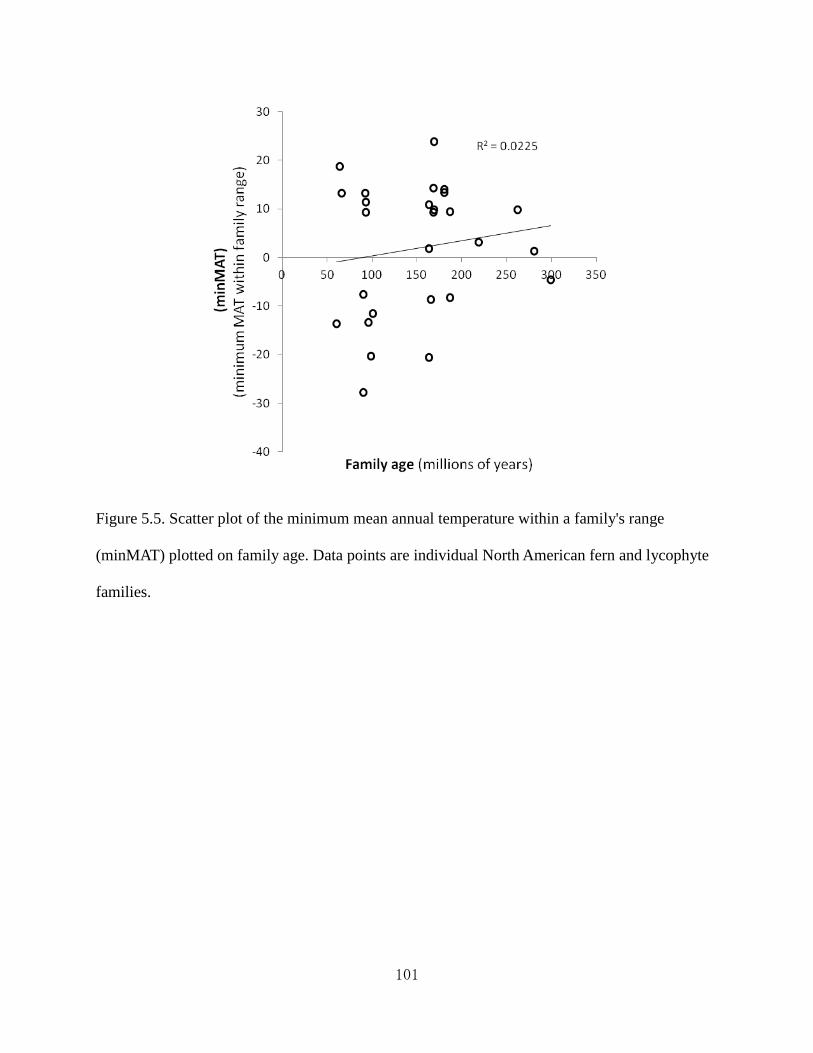
101
Figure 5.5. Scatter plot of the minimum mean annual temperature within a family's range
(minMAT) plotted on family age. Data points are individual North American fern and lycophyte
families.
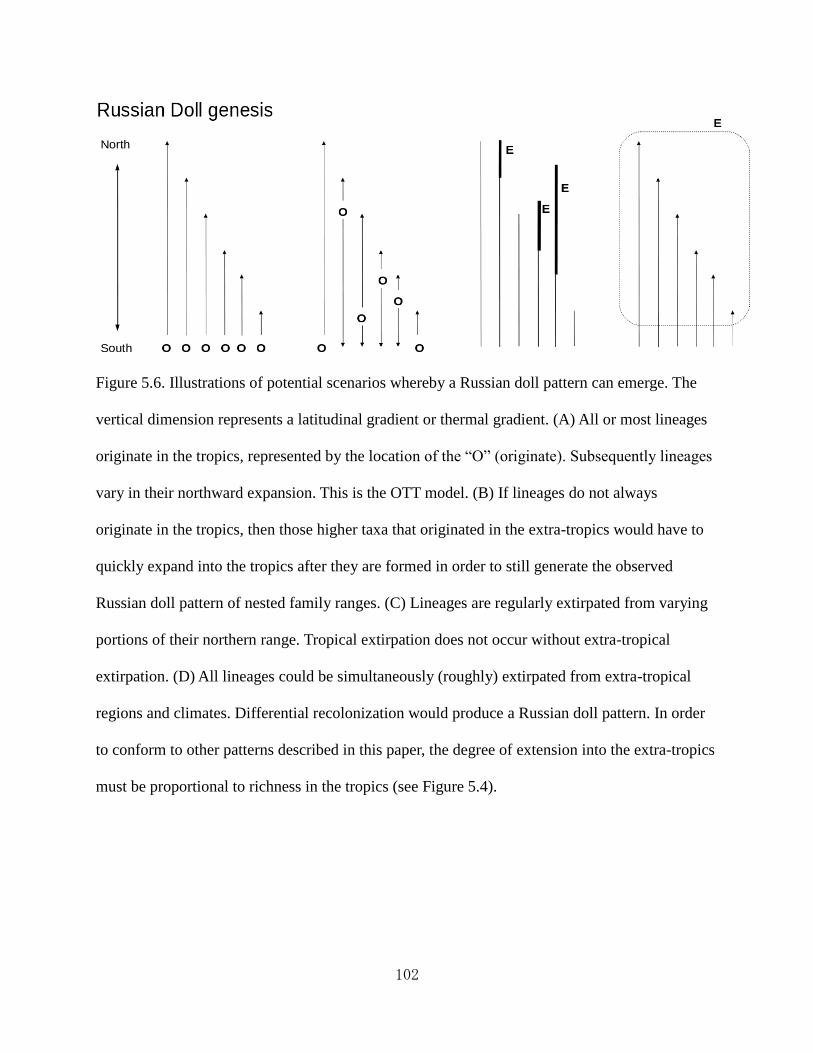
102
Figure 5.6. Illustrations of potential scenarios whereby a Russian doll pattern can emerge. The
vertical dimension represents a latitudinal gradient or thermal gradient. (A) All or most lineages
originate in the tropics, represented by the location of the “O” (originate). Subsequently lineages
vary in their northward expansion. This is the OTT model. (B) If lineages do not always
originate in the tropics, then those higher taxa that originated in the extra-tropics would have to
quickly expand into the tropics after they are formed in order to still generate the observed
Russian doll pattern of nested family ranges. (C) Lineages are regularly extirpated from varying
portions of their northern range. Tropical extirpation does not occur without extra-tropical
extirpation. (D) All lineages could be simultaneously (roughly) extirpated from extra-tropical
regions and climates. Differential recolonization would produce a Russian doll pattern. In order
to conform to other patterns described in this paper, the degree of extension into the extra-tropics
must be proportional to richness in the tropics (see Figure 5.4).

103
Chapter 6. The relationship between taxon richness and geographical breadth: a
biogeographical rule
Abstract
The relationship between family taxon diversity and spatial niche breadth is explored in
ferns, mammals, and amphibians. These patterns will be called diversity-expansion relationships.
Multiple measures of both taxon diversity and taxon expansion are employed. Strong
associations between diversity and expansion are found in all groups examined, and with all
diversity and expansion metrics. Major taxonomic groups differ from each other in their
relationships between diversity and expansion, having characteristic relationship slopes and
intercepts. Taxon diversity is correlated with taxon expansion regardless whether the lineage is
centered in the tropics or in temperate regions. The strong diversity-expansion relationships
suggest some kind of causal relationship exists between taxon diversification and large scale
geographical expansion; though direction and nature of causation remain undetermined. The
science of biogeography is likely to benefit from an understanding of this relationship.
Introduction
The following question motivates this study. Why do lineages differ in their geographical
breadth? Progress can be made by asking what attributes of a lineage are associated with lineage
geographical breadth (henceforth, expansion). In Chapter 5, taxon age was demonstrated not to
be a strong correlate with expansion. A taxon's diversity is another taxon attribute that could be
causally related to a taxon’s expansion. The relationship between a taxon's diversity and
geographical breadth will be referred to throughout as the diversity-expansion relationship,

104
where diversity refers to some aspect of the diversity of a taxon, and expansion refers to some
measurement of the spatial niche breadth of the taxon.
Species and populations are adapted to the abiotic and biotic conditions in the regions in
which they are found (Darwin, 1859; Wallace, 1878; Matyas, 1996; Nakazato et al. 2008).
Species will quickly diffuse to contiguous regions where they can persist and reproduce. To
expand beyond such regions, organisms must adapt to novel conditions (Mayr, 1963;
Antonovics, 1976). In this sense, why one lineage expands and why another does not is
fundamentally a question about why one lineage evolves and another does not. Diversification of
a taxon in place represents adaptation allowing wider niche breadth along multiple niche axes –
where the niche dimensions occur within a region. Expansion, on the other hand, involves a
similar process of niche expansion, but in this case the relevant niche dimensions correlate with
macrospatial gradients like latitude (for definition of the niche see Hutchinson, 1957). Therefore,
why lineages diversify could plausibly be related to why lineages expand geographically; both
are dependent on adaptive evolutionary change.
In this study expansion refers not merely to spatial extension of a lineage distribution, but
extension through a variety of conditions. Spatial niche breadth is the factor of interest herein;
ultimately, large scale geographical expansion requires evolutionary change to tolerate novel
conditions. I measure lineage expansion in several different ways (Table 6.1) in order to assess
generality of results. Diversity also will be estimated in several ways (Table 6.1).
Few studies have explored the relationship between taxon diversity and expansion. This
study addresses this need, making extensive comparisons of taxon richness and taxon expansion.
Recently generated species distribution databases, made by the author and others, allow more
extensive exploration of diversity-expansion patterns with finer resolution than previously

105
possible.
Family taxon richness and geographical/niche breadth could be related in a variety of
ways. These alternative relationships correspond to alternative evolutionary processes. Figure 6.1
(a-d) illustrates four alternative scenarios. Individual points represent higher taxa, such as
families. In the first scenario (Figure 6.1a) taxon geographical expansion (e.g., breadth on a
thermal niche gradient) is a strict function of the number of species in that lineage (taxon
richness). A lineage that does not diversify does not expand geographically and, conversely, a
lineage that increases in taxon richness necessarily expands into colder regions. Such a
relationship might be found if (a) The likelihood of an adaptive mutation allowing expansion
(occurring within any species within a family) increases with the number of species in the taxon.
More species simply means more chances for the occurrence of such events. Here, taxon
richness results in geographical expansion. (b) Alternatively, taxon expansion and diversity may
be two effects of the same cause. Namely, a taxon could possess a tendency for adaptive
evolution (evolvability; see Pigliucci, 2008) that results in both expansion and diversification.
A second scenario is illustrated in Figure 6.1b, where there is no strong relationship
between taxon richness and geographical expansion. This pattern would be expected if there
were no causal relationship (either directly or through another factor) between diversity and
expansion or if that relationship is obscured by other factors.
The remaining two scenarios are triangular relationships. Each lacks families in one
corner of the graph-space, the upper left or the lower right. In scenario three (Figure 6.1c)
families do not exist in the lower right region of the graph-space. These would be families with
high diversity and low expansion. High diversity may necessarily result in expansion, but
geographical expansion may not necessarily depend on high diversity.

106
In scenario four (Figure 6.1d) the upper left corner of the graph-space lacks families
rather than the lower right. Families in the lower right hand corner are families that have
diversified extensively but failed to expand. Widespread expansion may not be possible without
substantial diversification; however, diversification may not necessarily result in expansion. For
example, certain conditions, like cold temperatures, may present a hard constraint for a lineage.
There may be no possible evolutionary innovation that would allow a particular family of ferns
(a family of tree ferns for example) to persist in regions with a temperature below a particular
threshold. This family would then be constrained within a temperature isotherm. However, while
the lineage could not evolve a solution for survival and reproduction in cold temperature regions,
there is in principle no reason why it could not proliferate in place, within the tropical regions,
and realm where the lineage can persist.
To determine if diversity-expansion relationships observed in ferns generalize to other
major taxa, analyses were extended to other major taxa. When possible, all patterns were
evaluated first in ferns, but then additionally in mammals and amphibians. Ferns, mammals, and
amphibians are extremely different organisms, but they are similar in that to expand
geographically they must adapt to conditions alien to their present range. Thus, similar
relationships between diversity and expansion are possible, though likely with different
coefficients.
The quantity called “outside richness” is introduced in this study (see Table 6.1). Outside
richness is the number of species that aren't located in the peak richness region of the taxon
range. The peak or center of diversity of a lineage often corresponds to the center of origin of
that lineage (Cain, 1944; Ricklefs, 2006), if not in geographical space then at least in climate
niche space. This concept has been challenged by theoretical models (Goldberg et al., 2005), but

107
is certainly true in many circumstances, and is postulated as true herein. Outside richness can
thus be taken as an estimate of the number of species that are completely adapted to conditions
outside the center of origin of the lineage. Outside richness then is meant to be a very general
way of estimating the amount of expansion of a taxon.
Methods
The relationships between the diversity and expansion of North American ferns, New
World mammals, and global amphibians are explored predominantly with semi-log or log-log
scatter plots. Points in these relationships are individual higher taxa, usually families (but also
fern genera).
GIS range maps for most amphibian species (n = 6,148) were available on-line (IUCN,
2010). Species range maps were merged in GIS into 60 family range maps. New World mammal
species range maps were available on-line (Patterson et al., 2007). Some species range maps
were available as point files rather than species range polygons and these were not included in
analyses. In total 1,693 mammal species range maps were included in analyses. These were
merged into 59 family range maps using the classification scheme in the GIS database
(Patternson et al., 2007).
Relationships are expected to be characteristic for each larger taxonomic grouping
(typically orders). For example, constituent families of the mammal orders Rodentia,
Artiodactyla, and Chiroptera could have very different relationships between their diversification
and geographical expansion. Therefore, in many plots, families are colored by their order and
fitted with separate regression lines.

108
Spatial niche breadth
Expansion was measured in four ways (Table 6.1). (1) Latitudinal breadth is the range of
latitudes a family's range overlaps. This variable is a purely spatial variable. (2) Thermal niche
breadth is the range of temperatures encountered by the family within its range. Family range
maps were overlaid onto GIS climate maps of mean annual temperature MAT (sourced from the
Worldclim database, Hijmans et al., 2005) and minimum and maximum MAT (minMAT,
maxMAT; see Table 6.2 for a list of taxon thermal variables used in this study) within the range
were determined. Since most fern families extend into the tropics (warm temperatures), the
range of temperatures in which a fern family exists can be estimated by using the minimum
MAT (minMAT) found within that family's range. Many fern genera do not extend into warm
tropical regions, and so thermal niche range of fern genera must be determined by subtracting the
minMAT within the genus range from the maxMAT within the family range or from the peak
richness MAT (prMAT, see Table 6.2).
Thermal niche breadth was determined for fern families and fern genera only. Fern
species range maps use elevation range data (see Chapter 4) to produce more accurate range
maps from which thermal range can be realistically obtained. Maps of mammals and amphibians
are species range map polygons. However, comprehensive elevation data were not available for
mammals and amphibians, so good estimates of thermal niche breadth were not possible. For
these two taxa, latitudinal breadth, a coarse and indirect estimate of spatial niche, was used in
lieu of thermal niche breadth.
(3) For all groups, the number of ecoregions inhabited was used as an estimate of
expansion. This statistic was obtained by overlaying family range maps over a global ecoregion
map. A description of the ecoregions map and the criteria used to define ecoregions can be found

109
in Olson et al. (2001). Ecoregion number represents an index or composite estimate of taxon
environmental expansion along multiple biotic and abiotic niche gradients. Ecoregion number
contrasts with thermal niche breadth in that the latter represents expansion on a particular
(thermal) macrospatial niche gradient.
(4) Elevational extension data were available for fern families, and were an additional
estimate of spatial niche breadth probably similar to thermal niche breadth. Like thermal niche
breadth, maximum elevation can be used as a metric for elevational breadth for fern families,
because all fern families extend to lower elevations but vary in their maximum elevation.
Dispersal limitation may plausibly prevent a southern lineage from inhabiting colder northern
latitudes (though this is not the judgment of the author). However, dispersal limitation is much
less likely to prevent a lineage from expanding up an elevational gradient. If a lineage does not
persist at higher elevations within the tropics, this is unambiguously a consequence of a failure to
adapt to the colder conditions. The analysis of elevational extension is useful for this reason.
Finally, (5) outside richness, which is listed as a diversity variable in Table 6.1 can also be
thought of as an expansion measure, because outside richness is a measure of the number of
species that are completely adapted to conditions unlike the conditions in which the lineage
originated (center of diversity). The comparison between peak richness and outside richness is
considered to be a diversity-expansion comparison.
Diversity/Numbers
Diversity of taxa was estimated in several ways. (1) Taxon richness is simply the number
of species in the taxon (within the regions of analysis). (2) Peak richness, is the highest richness
observed for a family corresponding to usually one region in the world. Peak richness for fern

110
families and genera was estimated by overlapping all species ranges and identifying the region
with the most overlapping ranges (GIS union command). For mammals and amphibians, the
richness of each family was estimated on a 2-degree grid; peak richness was the number of
species in the richest 2-degree grid cell for each family. (3) Outside richness, described above, is
simply taxon richness minus peak richness.
(4) Peak N is the number of specimen records below the 25th
degree of latitude. Peak N is
intended to estimate the number of individuals of a higher taxon (family) present in tropical
regions of North America. This proxy is valid under the assumption that higher taxa that have
greater numbers of individuals are easier to find, and are also collected more frequently. The
number of specimen records is a crude estimate of family population size. Fern species specimen
records from Mexico, the continental U.S., Canada, and Greenland were accessed from the
Global Biodiversity Information Facility (GBIF), and grouped into GIS point shapefiles by
family. For each family, the number of specimens below 25 degrees north latitude was
determined in a GIS. Most fern families have richness centers below 25 degrees north so this
roughly corresponds to the number of individuals in the region of peak species richness of the
family.
Central diversification vs. horizontal expansion
I use comparisons of the following two variables, peak richness and outside richness, as
one manner of plotting and exploring diversity-expansion relationships (see Table 6.1). The peak
richness/outside richness dichotomy is essentially the most general manner of comparing
diversity vs. expansion; the comparison partitions all species in a taxon into those that increase
diversity in the geographical center and species that “explore” non-central space, or are

111
“expanders”. If the center of origin is inferred to be near the region of peak richness (see Cain,
1944), then species not present at the center of origin, have adapted to conditions unlike the
conditions in which the lineage originated.
Statistics
Throughout this study an emphasis is placed on multiple lines of evidence and generality
as a means of verifying patterns. Whenever possible, very large or comprehensive sample sizes
are obtained to dispel any doubt that patterns could be attributed to chance. Attention will be
given to high r-squared values.
Results
Taxon richness, peak richness, and thermal or latitudinal expansion
Fern family taxon richness predicts fern family minMAT (Figure 6.2; this figure is
identical to Figure 5.4). Since most fern families extend into the tropics and have peak richness
in the tropics (below 25N) the minimum MAT within the family range (minMAT) likely
estimates the lineage's total thermal niche expansion of most fern families. The highest richness
regions of some fern families are north of the 25th
parallel. These families are illustrated as filled
diamonds in Figure 6.2. Regression lines are fitted for both types of families (families with
tropical richness centers, r-squared = 0.651; families with temperate richness centers, r-squared =
0.516; all families, r-squared = 0.5403). Northern families tend to have lower minMAT than
tropical families for a given taxon richness, indicated by the lower intercept of the fit line.
Fern taxon peak richness also predicts taxon minMAT (Figure 6.3; families with tropical
richness centers, r-squared = 0.5730; families with temperate richness centers, r-squared =

112
0.6390; all families, r-squared = 0.4154). Thus, the number of species found at the region of peak
richness for a taxon predicts how expanded that lineage is in thermal niche space, usually
corresponding to locations thousands of kilometers distant from the peak richness region. For a
given peak richness, families with richness peaks in northern regions have extended further into
colder regions than families with tropical richness peaks.
For all mammal families the relationship between mammal family taxon richness and
latitudinal range (Figure 6.4) is moderate (r-squared = 0.2713). Using peak richness instead of
taxon richness the relationship is also moderate (r-squared = 0.2811). However, r-squared values
of this relationship are much stronger when evaluated for families of individual mammal orders
(Figure 6.4; Carnivora, r-squared = 0.8362; Artiodactyla, r-squared = 0.9051; Marsupials, r-
squared = 0.9753; Chiroptera, r-squared = 0.5336; Rodentia, r-squared = 0.2107; families from
other orders not including primates, r-squared = 0.6431). Given the strong relationship between
latitude and temperature, Figure 6.4 for mammals is comparable to Figures 6.2 and 6.3 for ferns.
Fern genera, like fern families display a relationship between taxon richness and thermal
expansion (Figure 6.5, r-squared = 0.5394). Several genera are outliers, as highlighted in Figure
6.5. R-squared values for the relationship are higher for particular families of genera than all
genera (Figure 6.6, Lycophytes, r-squared = 0.9298; Polypodiaceae, r-squared = 0.6345;
Pteridaceae, r-squared = 0.6380; Woodsiaceae, r-squared = 0.6409).
Fern family taxon richness and elevational extension
Fern family taxon richness is strongly associated with the taxon maximum elevation, (r-
squared = 0.4600). This relationship is much stronger for the largest order of fern families, the
Polypodiales (Figure 6.7, r-squared = 0.7933).
113
Central diversification vs. horizontal expansion
Taxon peak richness predicts taxon outside richness. Figures 6.8-6.10 plot peak richness
on outside richness, for North American ferns, New World mammals, and global amphibians. All
groups show similar patterns. The slope of the fit line tends to be greater than one. So families
with a large number of species at their richness center tend to have relatively more species
completely outside their richness center. This relationship is non-linear; a family that has a high
species richness peak tends to have a lot more species in total than a family with a low species
richness peak. The r-squared values are relatively high and characteristic for different orders
(Figure 6.11). The frog family Mantellidae, confined to Madagascar, is an outlier family with
lower outside richness than expected given its peak richness.
Diversity and expansion - Ecoregion expansion
Amphibian families with greater taxon richness or peak richness (Figures 6.12 and 6.13)
inhabit more ecoregions than amphibian families with lower diversity. Therefore, the use of
ecoregions as an estimate of expansion yields results similar to those observed in Figures 6.2 -
6.11. The Malagasy frog family, Mantellidae is an outlier in Figures 6.12 and 6.13 (as in previous
figures), occupying few ecoregions given its peak richness. Positive correlations also exist
between taxon richness and ecoregions for ferns (figure not shown; r-squared = 0.6783) and
mammals (figure not shown; r-squared = 0.3598).
Peak N and expansion
The number of herbarium records collected from a family below the 25th
parallel is a

114
good predictor of that family's minMAT (Figure 6.14). Fit lines were calculated for three groups,
families with temperate richness centers (r-squared = 0.6082), families with tropical richness
centers (r-squared = 0.4862), and families from the order Polypodiales (r-squared = 0.6826).
Peak N also predicts the latitudinal extent of taxa (r-squared = 0.3627).
Discussion
Results generally support scenario one (Figure 6.1a) as opposed to scenarios two, three,
or four (Figures 6.1b-d). For the organisms and phylogenetic scales evaluated, taxon diversity
and expansion are correlated without exception, though sometimes with considerable scatter.
These relationships are consistent across a variety of measures of diversity and expansion (Table
6.1). Thus, lineages that have failed to expand (either into new thermal zones, ecoregions, or
latitudes) but have diversified in place do not exist; lineages that expand in place (diversify)
always expand, both in space and in the range of environmental conditions tolerated.
The relationship between diversity and expansion is a general phenomenon not
specifically tied to the out of the tropics model (Chapter 5) or the latitudinal diversity gradient. In
Chapter 5, the pattern observed was that the amount of expansion from the tropics correlated
with taxon richness. Patterns outlined in this chapter, demonstrate that the amount of expansion
(regardless where the lineage is centered) correlates with taxon diversity, not the amount of
extension from the tropics per se. Several mammal families are not tropical, and it is their
latitudinal ranges rather than their extension from the tropics correlates with their taxon richness
(Figure 6.4). Similarly, not all fern genera have their richness peak in the tropics. Fern genus
taxon richness correlates with genus thermal range, regardless whether the lineage is centered in
the tropics or temperate region (Figures 6.5 and 6.6). Fern families with temperate richness peaks

115
extend into colder regions for a given level of richness than families with their center in the
tropics (Figures 6.2 and 6.3).
The absence of lineages that fail to expand if they diversify falsifies scenario four. This
pattern suggests something about the long term evolutionary capacity of lineages, at least as it
relates to terrestrial biogeography. Conceivably, a taxon or family could exist that had very little
chance to evolve a set of integrated adaptations required for expansion beyond a particular
isotherm. In other words, a taxon may possess a constraint on its evolutionary potential in a
particular niche dimension (e.g. a thermal gradient). This phenomenon of evolutionary limitation
probably does occur. A plausible example may be plants with respect to marine environments.
Plants (and many constituent taxa) have diversified extensively, but none have succeeded in
extensively occupying marine environments. However, within the theater of the terrestrial
environment, the relationship between diversity and expansion suggests that such constraints do
not exist. If a lineage is able to diversify in place, that lineage will inevitably achieve an adaptive
solution allowing expansion on a thermal gradient.
Diversity-expansion patterns strongly suggest that causal relationships exist between
taxon diversity and taxon geographical expansion. Contrary to the aphorism “correlation does
not imply causation”, correlation does provide a strong hint of causal relationships, at least
through common cause if not more directly (Tufte, 2003). Nonetheless, directions of causality
remain unknown.
The existence of the outlier frog family Mantellidae (Figures 6.10, 6.12, and 6.13) is
interesting for the following reason. By being restricted to the island of Madagascar, this lineage
is in a sense artificially restricted in its expansion. However, this lineage is nonetheless able to
diversify in place (proliferate “vertically”). This suggests that lineages do not need to undergo

116
horizontal geographical expansion to diversify. So either diversity causes expansion or a third
variable such as evolvability causes both. This does resolve some questions about potential
causal relationships.
Elevational extension was among the tested expansion metrics (Table 6.1). Dispersal
limitation is much less likely to prevent a family from expanding up an elevational gradient than
a latitudinal or continental thermal gradient. Yet, the diversity-expansion pattern exists in both
cases (with expansion measured along a latitudinal or elevational gradient). Dispersal limitation
is not a likely explanation for either pattern (especially for widely dispersing ferns); instead
parsimony suggests that both patterns are due to similar evolutionary causes. Variation between
lineages in the quantity of accrued adaptive evolution can explain both patterns; dispersal
limitation cannot.
Results are characteristic for different groups (Figures 6.4, 6.6, 6.8-6.11, 6.14). This is
especially true for mammals (Figure 6.4). As lineages undergo adaptive evolutionary
geographical expansion, reproductive isolation may occur at characteristic intervals in
geographical or environmental niche space. For rodents due to their short dispersal distances,
that distance may be short. For Artiodactylans, or Chiropterans, that distance may be long. Thus
one would expect a larger number of rodent species than bat species, given a particular level of
adaptive evolutionary geographical expansion. This is what is observed in Figure 6.4.
An interesting pattern is apparent in Figure 6.11. The positions of fit lines in Figure 6.11
are roughly proportional to the likely dispersal capacity of these higher taxonomic groups. Fit
lines from Figures 6.8-6.10 are superimposed onto Figure 6.11 to illustrate this pattern. Highly
dispersing taxa - bats and polypod ferns - have the lowest positions in Figure 6.11;
Artiodactylans are in between Polypodiales and bats. Carnivorans and marsupials have the next
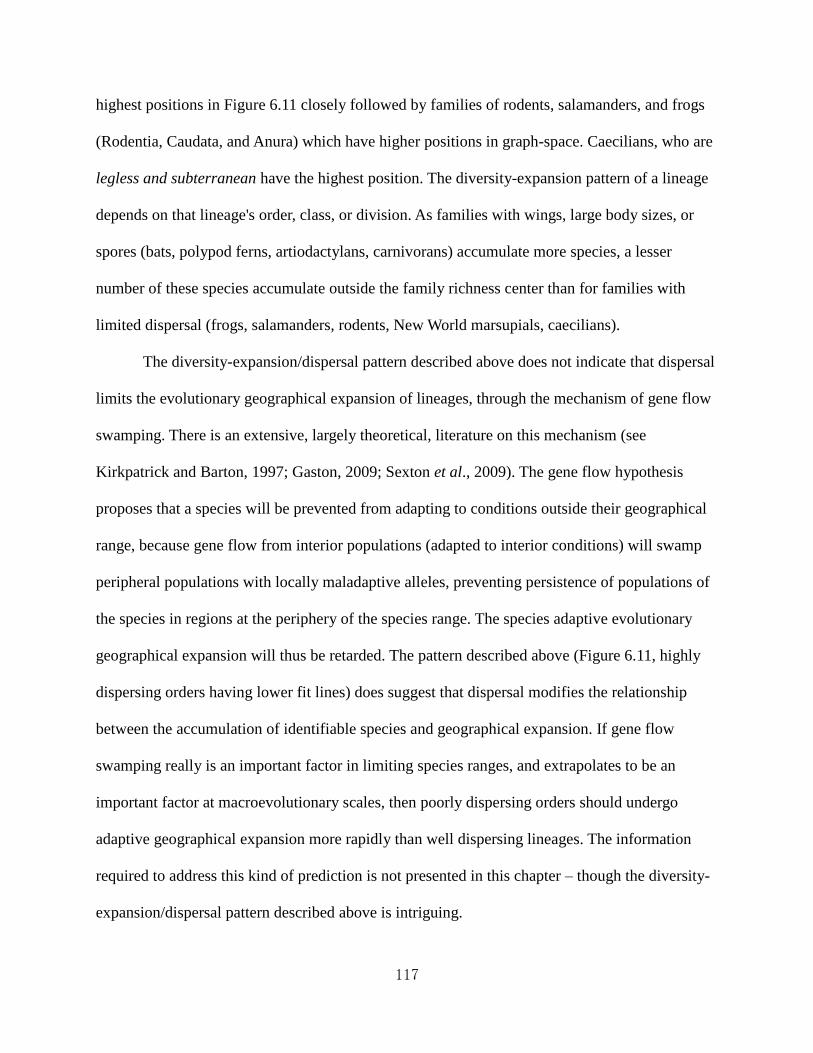
117
highest positions in Figure 6.11 closely followed by families of rodents, salamanders, and frogs
(Rodentia, Caudata, and Anura) which have higher positions in graph-space. Caecilians, who are
legless and subterranean have the highest position. The diversity-expansion pattern of a lineage
depends on that lineage's order, class, or division. As families with wings, large body sizes, or
spores (bats, polypod ferns, artiodactylans, carnivorans) accumulate more species, a lesser
number of these species accumulate outside the family richness center than for families with
limited dispersal (frogs, salamanders, rodents, New World marsupials, caecilians).
The diversity-expansion/dispersal pattern described above does not indicate that dispersal
limits the evolutionary geographical expansion of lineages, through the mechanism of gene flow
swamping. There is an extensive, largely theoretical, literature on this mechanism (see
Kirkpatrick and Barton, 1997; Gaston, 2009; Sexton et al., 2009). The gene flow hypothesis
proposes that a species will be prevented from adapting to conditions outside their geographical
range, because gene flow from interior populations (adapted to interior conditions) will swamp
peripheral populations with locally maladaptive alleles, preventing persistence of populations of
the species in regions at the periphery of the species range. The species adaptive evolutionary
geographical expansion will thus be retarded. The pattern described above (Figure 6.11, highly
dispersing orders having lower fit lines) does suggest that dispersal modifies the relationship
between the accumulation of identifiable species and geographical expansion. If gene flow
swamping really is an important factor in limiting species ranges, and extrapolates to be an
important factor at macroevolutionary scales, then poorly dispersing orders should undergo
adaptive geographical expansion more rapidly than well dispersing lineages. The information
required to address this kind of prediction is not presented in this chapter – though the diversity-
expansion/dispersal pattern described above is intriguing.
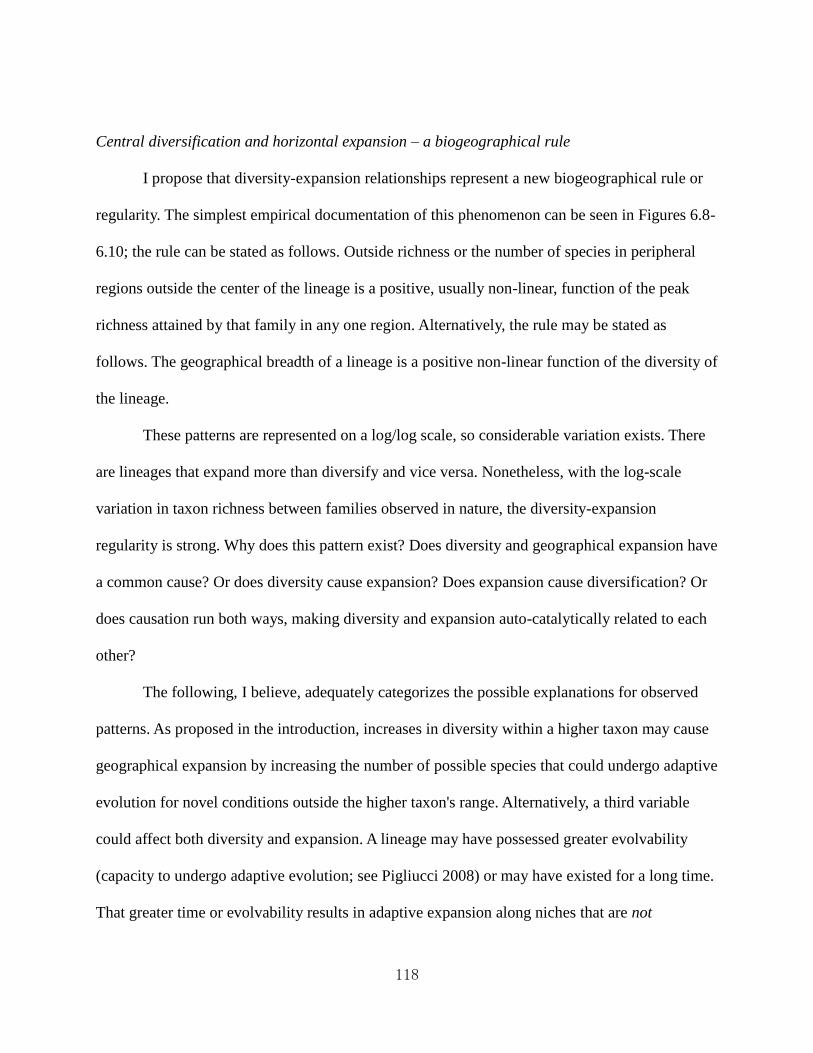
118
Central diversification and horizontal expansion – a biogeographical rule
I propose that diversity-expansion relationships represent a new biogeographical rule or
regularity. The simplest empirical documentation of this phenomenon can be seen in Figures 6.8-
6.10; the rule can be stated as follows. Outside richness or the number of species in peripheral
regions outside the center of the lineage is a positive, usually non-linear, function of the peak
richness attained by that family in any one region. Alternatively, the rule may be stated as
follows. The geographical breadth of a lineage is a positive non-linear function of the diversity of
the lineage.
These patterns are represented on a log/log scale, so considerable variation exists. There
are lineages that expand more than diversify and vice versa. Nonetheless, with the log-scale
variation in taxon richness between families observed in nature, the diversity-expansion
regularity is strong. Why does this pattern exist? Does diversity and geographical expansion have
a common cause? Or does diversity cause expansion? Does expansion cause diversification? Or
does causation run both ways, making diversity and expansion auto-catalytically related to each
other?
The following, I believe, adequately categorizes the possible explanations for observed
patterns. As proposed in the introduction, increases in diversity within a higher taxon may cause
geographical expansion by increasing the number of possible species that could undergo adaptive
evolution for novel conditions outside the higher taxon's range. Alternatively, a third variable
could affect both diversity and expansion. A lineage may have possessed greater evolvability
(capacity to undergo adaptive evolution; see Pigliucci 2008) or may have existed for a long time.
That greater time or evolvability results in adaptive expansion along niches that are not

119
correlated with macrospatial dimensions, resulting in diversification within the center of origin
of the lineage. Simultaneously, populations (eventually being recognized as new species) with
capacity for adaptive evolution (bestowed by time or evolvability) would also expand on niche
dimensions that are correlated with macrospatial dimensions (adaptation to novel conditions
outside the taxon range). I hypothesize that diversity-expansion relationships exist because both
diversification and geographical expansion and are dependent on the same phenomenon,
adaptive evolution along niche dimensions (Hutchinson, 1957).
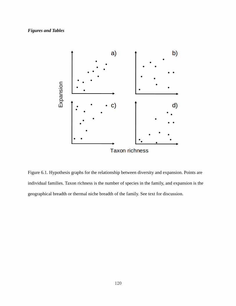
120
Figures and Tables
Figure 6.1. Hypothesis graphs for the relationship between diversity and expansion. Points are
individual families. Taxon richness is the number of species in the family, and expansion is the
geographical breadth or thermal niche breadth of the family. See text for discussion.

121
Figure 6.2. Relationship between a North American fern family's taxon richness and the
minimum mean annual temperate within its range (minMAT). Data are from North America
(Mexico, Continental United States, Canada, and Greenland). Since all families extend into the
warm areas (Chapter 5) minMAT is an estimate of total amount of thermal niche expansion of a
family. Points represent individual North American fern families. Open circles represent families
with peak richness centers in tropical latitudes. Solid black diamonds represent families that have
richness centers in temperate latitudes.

122
Figure 6.3. This graph is similar to Figure 6.2 except that peak richness is plotted on the x-axis
instead of taxon richness.

123
Figure 6.4. Mammal family latitudinal range plotted on mammal family taxon richness. Data are
from the New World. Points represent individual New World mammal families. Regression fit
lines are plotted for different orders or higher taxonomic groupings of mammal families
(Marsupials, Artiodactyla, Carnivora, Chiroptera, Rodentia, and other non-primate mammal
families).

124
Figure 6.5. Thermal range of individual North American fern genera plotted on taxon richness
(of each genus). Points represent individual North American fern genera. Thermal range is
estimated here as genus prMAT – minMAT (mid-value mean annual temperature of the genus
richness peak minus the minimum mean annual temperature within the genus range).

125
Figure 6.6. North American fern genera thermal range plotted on taxon richness (of each genus).
Points represent individual fern genera. Thermal range is estimated here as genus prMAT –
minMAT, the difference between the lowest MAT within a genus range, and the mid-value MAT
value of the region of peak richness for the genus. Genera are colored by larger taxonomic
groupings. Regression fit lines are plotted for these larger taxa.

126
Figure 6.7. Maximum elevation on taxon richness of North American families from the order
Polypodiales.

127
Figure 6.8. Outside richness on peak richness of North American fern families. A fit line is
plotted for all families (black). Families of the Polypodiales are colored orange and fitted with a
separate regression fit line (orange).
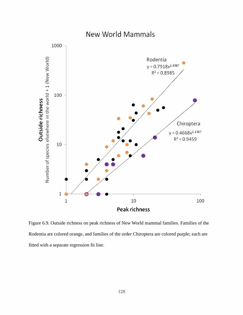
128
Figure 6.9. Outside richness on peak richness of New World mammal families. Families of the
Rodentia are colored orange, and families of the order Chiroptera are colored purple; each are
fitted with a separate regression fit line.

129
Figure 6.10. Outside richness on peak richness of global amphibian families. Families of Anura
(frogs) are colored green, families of Caudata (salamanders) are colored red, and families of
Gymnophiona (caecilians) are colored blue; each are fitted with a separate regression fit line.
Note that the Mantellidae a family of frogs endemic to Madagascar is an outlier, with lower
outside richness than expected given the peak richness of the family.

130
Figure 6.11. Outside richness on peak richness. This is a composite graph of families plotted in
Figures 6.8-6.10. Individual families (points) are not shown, instead regression fit lines of many
higher taxonomic units are plotted together. R-squared values for each regression fit line are
provided at right.

131
Figure 6.12. Number ecoregions inhabited on taxon richness of global amphibian families. Note
again, that the Mantellidae family is an outlier, inhabiting fewer ecoregions than expected given
its taxon richness.

132
Figure 6.13. Similar to Figure 6.10. except that peak richness rather than taxon richness is plotted
on the x-axis.

133
Figure 6.14. minMAT on peak N of North American fern families (monilophytes). Peak N is the
number of GBIF herbarium records. Peak N is thought to represent a rough indicator of number
of individuals of the family from the tropical region. For most families the tropical region
corresponds to the region of peak species richness. Families with richness peaks in temperate
regions are colored green, and are plotted with a separate regression fit line. All other families
(black and orange points) have tropical richness peaks and are plotted with a regression fit line
(black). The orange points are families of the Polypodiales.

134
Table 6.1. Taxon diversity and expansion variables used in this study. Outside richness as
described in the text could be thought of as both a diversity variable and an expansion variable.
Table 6.2. Taxon thermal variables. Temperatures are expressed in degrees Celsius.

135
Chapter 7. Discussion
In this final chapter I will summarize major findings. What have we learned? How can we
interpret the diverse set of geographical patterns and results presented in this dissertation? I'll
provide an overview and develop a narrative in order to address these questions. I'll do so by
returning to the research themes presented in the introduction (Chapter 1). Special attention will
be placed on geography as a lens for evolution.
Geography as a lens for Macroevolution
“Geography as a lens for evolution” was presented as a research theme in the
introduction. I'll suggest now that the biogeographical patterns studied in this dissertation speak
mostly on macroevolution. Macroevolution can be defined as evolution at or above the species
level. This dissertation largely focused on continental to global geographical scales, and
phylogenetic scales corresponding to class or division levels. The evolution of these lineages
over these spaces takes place over tens and hundreds of millions of years. Every chapter in this
dissertation involved many species. Graphs, maps, and tables presented species, regions, or even
higher taxa as the underlying data points. The analysis of patterns at such scales will be useful
for providing insights into macroevolution.
Microevolutionists have identified a diverse range of evolutionary processes. The job of a
macroevolutionist or biogeographer is in part to identify which processes operate most
frequently, which processes are most important, or most dramatically contribute to observed
patterns over such immense distances and time. Several scholars have argued that some
phenomena exist exclusively at immense scales, and cannot be studied at microevolutionary
scales (Stanley, 1975; Lloyd and Gould, 1993; Lieberman and Vrba, 1995; Gould and Lloyd,

136
1999; Jablonski, 2000; Jablonski, 2007; Jablonski, 2008; Pigliucci, 2008; see Pigliucci, 2010).
This debate will not be entered into. Suffice it to say that even if macroevolutionary processes
and macrogeographical patterns are straightforward cumulations of microevolutionary processes,
outcomes at broad-scales will still exist that are not predictable from our knowledge at micro-
scales. Determining what microevolutionary mechanisms operate to produce broad-scale
patterns, and what broad-scale patterns microevolutionary mechanisms will produce, are distinct
problems from the original identification and description of the microevolutionary mechanisms.
Biogeographers and macroevolutionists may begin analyses with the descriptive approach of
identifying the endpoint biotic patterns. I will now go through the chapters, and present what I
believe are the most important biogeographical and macroevolutionary insights.
Chapter 2.
The second chapter demonstrates that North American fern and lycophyte richness are
highly related to two very simple climatic variables, mean annual temperature (MAT) and
rainfall (RAN). This result is not at all novel, and in line with similar observations in other taxa
and ferns elsewhere in the world, including regions like Australia (Bickford and Laffan, 2006)
with very different histories and spatial arrangements of climatic conditions. That similar
biogeographical relationships emerge in regions with different histories and geographies suggests
that universal processes operate to produce the latitudinal diversity gradient (Krug et al., 2009).
However, one result from Chapter 2 was not expected and is not easy to put into context. The
correlation between climatic variables and fern species richness is lower than the correlation
between these climatic variables and fern family richness.

137
Chapter 3.
Researchers have speculated that polyploid species have high evolutionary capacity due
their extra compliment of genes. Within the third chapter scrutiny was placed on this idea using
comprehensive geographical evidence. My collaborator Michael Barker and I found that the
number of polyploid species found in a region is predicted by extant opportunities for polyploid
species formation. Allopolyploid richness is a function of the number of congeners present in a
location that could potentially combine to produce an offspring allopolyploid. Rather than
suggesting that a typical polyploid species has great evolutionary capacity, this result is instead
consistent with a scenario where many polyploids exist largely due to continual formation.
However, we speculate that the long term implications of polyploidy on plant evolution may be
the result of exceptional polyploid species that do survive well beyond initial formation.
Chapter 4.
The primary purpose of the fourth chapter was the construction and evaluation of a North
American fern and lycophyte distribution database. The constructed GIS database utilized
species range data and elevational range data in combination to produce more refined estimates
of species distribution. The resulting GIS database was used to estimate thermal niche
parameters of fern families. Despite the utilitarian purpose of this chapter, several things are
learned from the success of the database in its purposes. Humboldt (1805) described a regular
species latitude-elevation distributional pattern, where species at temperate latitudes at sea-level
would exist at predictable elevational levels as one moves toward the equator. The analyses in
Chapter 4 demonstrate that the relationship fern taxa have with climate and elevation is highly
regular. Finally, Chapter 4 demonstrates that required data exist for comprehensive evaluations of

138
climate niche evolution.
Chapter 5.
The fifth chapter returns to continental scale richness patterns of North American ferns
and lycophytes but explores beyond simply the geographical variation in total numbers of
species. The primary question driving the study was the following. What is the pattern of
evolutionary construction of the latitudinal diversity gradient (LDG)? The out of the tropics
(OTT) model developed by Jablonski (1993) served as the model to address the question. Results
were striking. The great regularities in the distribution of numbers of fern species with respect to
climate found in Chapter 2 are mirrored by great regularities in the numerical and distributional
structure of fern lineages from which those numbers are drawn. Fern families display a nearly
perfect nested structure with all families rooted in warm and wet south tropical areas. Moving
away from these regions fern families are continually lost, without gaining new endemic
temperate families. Two alternative models were presented explain the observed patterns: the
OTT model and tropical conservatism hypothesis (TCH). The demands on explanations for the
LDG are now higher, such explanations must conform to a highly ordered biotic pattern.
Chapter 6.
Chapter 6 contains a documentation and description of diversity-expansion relationships.
Family taxon richness (or peak richness) is correlated with family geographical breadth. For a
particular order of families the relationship between these two variables is often strong. This
represents a global and continental biogeographical regularity, and it is observed among North
American ferns, New World mammals, and global amphibians - all taxa examined in Chapter 6.

139
Diversity-expansion relationships illustrate a global picture of evolution. Diversity-
expansion relationships suggest something about lineages that are going extinct, or decreasing in
relative number. Not all lineages are positively expanding. Which particular lineages are
retracting (negative expansion) may be unknown. However, the fact that the relationship between
taxon richness and geographical breadth is maintained for almost all higher taxa examined
demonstrates that retracting lineages have a particular pattern of retraction that mirrors the
pattern of expansion observed in other lineages. Peripheral elements of a family are extirpated
first, while simultaneously the central diverse region of a family decreases in number as well.
This kind of pattern is understandable when looking at biogeography as a process of adaptive
evolution over space. The central lineages have existed for a longer time in central region
environments than peripheral lineages have existed in peripheral environments. Central lineages
therefore could be expected to be more finely adapted to their environment than peripheral
lineages, and therefore the last to disappear in a long-term competitive struggle with adjacent
life.
What about higher taxa that are in the process of expanding? Higher taxa that are
successful in the production of new species in their (referring to higher taxa) peripheral
environments, are presumably successful at producing new adaptive phenotypic variety.
Geographical expansion into alien environments requires adaptive evolution (Mayr, 1963;
Antonovics, 1976; Griffith and Watson, 2006). Higher taxa that successfully expand beyond their
periphery could be expected to originate new higher taxa as well; originations may often take
place in a higher taxon's central regions where most of the species of the taxon reside.
Diversity-expansion graphs in Chapter 6 can be understood as snap-shots of the
evolutionary process, with higher taxa in different stages of their ontogeny. Some lineages are

140
retracting, slowly decreasing in diversity, in geographical breadth, and in absolute number of
individuals. Other lineages are recently originated, most frequently in the tropics but
occasionally elsewhere, and are beginning their increase in diversity, breadth, and numbers.
Finally, some lineages have expanded greatly in all dimensions, and are generating high species
diversity that in time would generate the new phenotypic diversity that eventually would be
recognized as new families by biologists in the future. These new families would again begin an
expansion process. Preliminary results indicate that the diversity, geographical breadth, and
absolute number of individuals of a taxon are associated with a fourth variable, taxon
morphological breadth (in preparation). Again, these observations point to a picture of
biogeography as a process of adaptive evolution over space.
What causes diversity-expansion relationships is unknown, though there are several
possibilities. A lineage might expand while others do not because one lineage has an advantage
over others. Two kinds of advantages come to mind. (1) A lineage could possess greater capacity
to generate adaptive variation (greater evolvability). (2) Or a lineage could possess a “general
adaptation” (see Darlington, 1959). A general adaptation is useful in all or most environments
and can be contrasted with a specific adaptation which is useful in particular environments only.
Lineages with general adaptations would have general competitive advantages over other
lineages. In other words one lineage could be universally competitively dominant over others,
and over time expand at the expense of competitors.
Diversity-expansion relationships could also emerge randomly. Imagine two species,
species A and B, each the progenitor of a future family (family A and B). Species A may produce
a new species entirely by chance. At this stage the family founded by species A, family A, now
has a greater chance of producing a third species by virtue of having two species. Family A also

141
now has a greater chance of acquiring an adaptive mutation or mutations that will allow
geographical expansion. This process could be expected to lead to great asymmetries between
families simultaneously in their diversity, geographical breadth, numbers, and phenotypic range.
Diversity-expansion patterns could be caused by random processes or may result from
differences between lineages in evolvability or dominance. At the moment, the underlying cause
of diversity-expansion patterns is not determined. Nonetheless, the results do show that what
must be explained is a whole syndrome of expansion or retraction on multiple variables.
Diversity-expansion patterns in historical context
I'll now provide a short historical note in order to gain insight on how to proceed in the
analysis of diversity-expansion relationships. I argue that Darwin identified some patterns that
are related to or are examples of diversity-expansion relationships. Darwin developed concepts
related to long-term evolution surrounding his empirical work on “botanical arithmetic”
(Browne, 1980). Darwin's work and views on botanical arithmetic have been largely overlooked
because they receive only a brief treatment in Chapter 2 of the Origin of Species (Tammone,
1995). This contrasts with the time spent on these questions in his “big species book”, Natural
Selection, in which Darwin had written nearly fifty pages of notes on the subject.
Darwin saw continuity between varieties, populations, and species (Mayr, 1992). This
perspective in addition to Darwin's principle of divergence was rejected by evolutionists in the
late 20th century (Mayr, 1992; Mallet, 2010; Schemske, 2010). However, recently some
researchers are returning to views on species, ecotypes, and divergence similar to Darwin's
(Schemske, 2010; Lowry, 2012). Because of Darwin's view on variation and species, he saw
continuity between the ability to generate adaptive variation and the ability to generate new
142
species. Darwin (1859, pg. 156) expressed the belief that common lineages were common because
they were able to generate great variation.
...the more diversified the descendants from any one species become in structure, constitution, and habits,
by so much they will be better enabled to seize on many and widely diversified places in the polity of
nature, and so be enabled to increase in numbers.
Darwin turned to botanical arithmetic to explore these ideas empirically (Browne, 1980).
He observed that species with varieties tend to be in genera with many species. These varieties,
so the argument went, were in the process of forming incipient species. To Darwin, the presence
of varieties in a species within a genus and the large number of species in the genus were linked
facts. Genera that were producing many new varieties and species were colorfully referred to as a
manufactory of species. The manufactory of species hypothesis has been tested recently with
birds and results are consistent with the hypothesis (Haskell and Adhikari, 2009). Using genera
as higher taxa for comparison Darwin made several comparisons of species number,
geographical breadth, and commonness (which can be taken as a proxy for absolute number of
individuals). For example, in one analysis he found that genera that contain common species had
on average four species, while genera without common species had on average 1.8 species
(Browne, 1980; Stauffer, 1975). Darwin also compared geographical range size to commonness
and found a slight association. The ability to generate adaptive variation was seen as the cause
underlying the association between these three attributes: diversity, commonness, and
geographical breadth.
Darwin clearly believed that higher taxa varied in their capacity to generate adaptive
variation and that this capacity was heritable within a higher taxon like a genus (Darwin, 1859;

143
Chapter 2). This capacity might be labeled evolvability in the contemporary vocabulary. Darwin,
like Darlington, (1959) also believed that some taxa were competitively superior or dominant
over others, and that this dominance would facilitate diversification, expansion, and numerical
proliferation of such taxa. Regardless whether randomness, evolvability, or competitive
superiority drive diversity-expansion relationships, contemporary databases and processing
technology will allow a more comprehensive exploration of these problems. As diversity-
expansion relationships are explored further, Darwin's concepts regarding long term evolution
should receive renewed scrutiny.
Dispersability and family geographical breadth
Fern dispersability has been highlighted repeatedly throughout this dissertation. There are
reasons to believe other groups have the ability to disperse to appropriate environments within
contiguous regions on continents even though they do not disperse via microscopic spores. The
only families that are outliers in the diversity-expansion biogeographical rule described in
Chapter 6, are amphibian lineages located on the Seychelles and Madagascar. These islands are
formerly part of continental Gondwanaland. The amphibian families inhabiting these landmasses
are unable to disperse to the contemporary continents of Asia or Africa given the great distances
involved. Nonetheless, they continue to diversify in place. If a lineage diversifies on a continent,
that lineage expands geographically. These observations suggests that dispersal limitation does
not typically restrict a fern, mammal, or amphibian family from geographical expansion. Instead
if a family does fail to expand this is related to its failure to diversify.

144
Final thoughts
Many results presented in this dissertation are macroevolutionary regularities - highly
non-random outcomes not directly prescribed from microevolutionary theories. For example, in
Chapter 2, further evidence is provided for a global climate-richness relationship. Non-random
and repeated regularities point to particular kinds of generalizations regarding the evolutionary
process at broad-scales. Historical vicissitudes while important, are not consequential enough to
disrupt the generation of regularities. Macroevolution appears instead to be predictable, with
coordinated change in lineages in multiple dimensions.
Macroevolutionary concepts, due to their scale, may not be easily amenable to many tools
of the scientific methods. This does not mean that such scales are not amenable to systematic
reflection. And with large collections of data at global scales, the situation can change.
How, for example, will ultimate explanation be found for the diversity-expansion
relationship observed and described in Chapter 6? Theories will need to be developed that
specify the component forces and processes that give rise to such a global scale regularity. We
may already know much about the possible candidate forces, but we do not have an answer for
how these forces operate together or individually to manifest the global patterns we observe.
The analyses in this dissertation have allowed me to make positive and plausible
statements regarding what typically happens to a polyploid species, or what we can expect of the
geographical expansion (or retraction) of a lineage given a specified amount of diversification
(or extinction). Such statements would not be possible without a biological research strategy
aimed at comprehensiveness, its requisite available global data, technology for collating such
data, and people willing to do the necessary work.

145
References
Aldasoro, J.J., Cabezas, F., and Aedo, C. (2004) Diversity and distribution of ferns in Sub-
Saharan Africa, Madagascar and some islands of the South Atlantic. Journal of
Biogeography, 31 (10): 1579-1604.
Allen, A.P., and Gillooly, J.J. (2006) Assessing latitudinal gradients in speciation rates and
biodiversity at the global scale. Ecology Letters, 9 (8): 947-954.
Antonovics, J. (1976) The nature of limits to natural selection. Annals of the Missouri Botanical
Garden, 63 (2): 224-247.
Balmford, A., Green, M.J.B., and Murray, M.G. (1996) Using higher-taxon richness as a
surrogate for species richness. 1. Regional tests. Proceedings of the Royal Society of
London. Series B: Biological Sciences, 263: 1267-1274.
Barker, M.S., Kane, N.C., Matvienko, M., Kozik, A., Michelmore, R.W., Knapp, S.J., and L.H.
Rieseberg (2008) Multiple paleopolyploidizations during the evolution of the compositae
reveal parallel patterns of duplicate gene retention after millions of years. Molecular
Biology and Evolution, 25 (11): 2445-2455.
Barker, M.S., Vogel, H., and Schranz, M.E. (2009) Paleopolyploidy in the brassicales: analyses
of the cleome transcriptome elucidate the history of genome duplications in arabidopsis
and other brassicales. Genome Biology and Evolution, 1 (1): 391-399.
Barker, M.S., and Wolf, P.G. (2010) Unfurling fern biology in the genomics age. BioScience, 60:
177-185.
Barrington, D.S. (1993) Ecological and historical factors in fern biogeography. Journal of
Biogeography, 20: 275-279.

146
Behrensmeyer, A.K., Damuth, J.D., DiMichele, W.A., and Potts, R. eds. (1992) Terrestrial
ecosystems through time: evolutionary paleoecology of terrestrial plants and animals.
University of Chicago Press, Chicago.
Beyer, H.L. (2004) Hawth's Analysis Tools for ArcGIS. Available at
http://www.spatialecology.com/htools.
Bhattarai, K.R., Vetaas, O.R., and Grytnes, J.A. (2004) Fern species richness along a central
Himalayan elevational gradient, Nepal. Journal of Biogeography, 31: 389-400.
Bickford, S.A., and Laffan, S.W. (2006) Multi-extent analysis of the relationship between
pteridophyte species richness and climate. Global Ecology and Biogeography, 15: 588-
601.
Birks, H.J.B. (1976) Distribution of European pteridophytes - numerical-analysis. New
Phytologist, 77: 257-287.
Blanc, G., and Wolfe, K.H. (2004) Widespread paleopolyploidy in model plant species inferred
from age distributions of duplicate genes. The Plant Cell, 16 (7): 1667-1678.
Bolstad, P. (2005) GIS fundamentals: A first text on geographic information systems, 2nd
edition. Eider Press, White Bear Lake, MN.
Bradshaw, A.D. (1991) Genostasis and the limits to evolution. Philosophical Transactions of the
Royal Society of London. Series B: Biological Sciences, 333 (1267): 289-305.
Bridle, J.R., and Vines, T.H. (2007) Limits to evolution at range margins: when and why does
adaptation fail? Trends in Ecology & Evolution, 22 (3): 140-147.
Briggs D., and Walters, S.M. (1997) Plant Variation and Evolution, 3rd
edition. University Press,
Cambridge.
Brown, J.H. (1995) Macroecology. University of Chicago Press, Chicago.

147
Brown, J.H., and Maurer, B.A. (1989) Macroecology: the division of food and space among
species on continents. Science, 243 (4895): 1145-1150.
Browne, J. (1980) Darwin's botanical arithmetic and the principle of divergence, 1854-1858.
Journal of the History of Biology, 13 (1): 53-89.
Cain, S.A. (1944) Foundations of plant geography. Harper and Brothers, New York.
Cardillo, M. (1999) Latitude and rates of diversification in birds and butterflies. Proceedings of
the Royal Society of London. Series B: Biological Sciences, 266 (1425): 1221-1225.
Cardillo, M., Orme, C.D.L., and Owens, I.P.F. (2005) Testing for latitudinal bias in
diversification rates: an example using New World birds. Ecology, 86 (9): 2278-2287.
Cui, L., Wall, P.K., Leebens-Mack, J.H., Lindsay, B.G., Soltis, D.E., Doyle, J.J., Soltis, P.S.,
Carlson, J.E., Arumuganathan, K., Barakat, A., Albert, V.A., Ma, H., and dePamphilis,
C.W. (2006) Widespread genome duplications throughout the history of flowering plants.
Genome Research, 16 (6): 738-749.
Currie, D.J. (1991) Energy and large-scale patterns of animal-species and plant-species richness.
American Naturalist, 137: 27-49.
Currie, D.J., and Paquin, V. (1987) Large-scale biogeographical patterns of species richness of
trees. Nature, 329: 326-327.
Darlington, P.J. (1959) Area, climate, and evolution. Evolution, 13 (4): 488-510.
Darwin, C. (1859) On the origin of species by means of natural selection. J. Murray, London.
Elith, J., Graham, C.H., Anderson, R.P., Dudík, M., Ferrier, S., Guisan, A., Hijmans, R.J.,
Huettmann, F., Leathwick, J.R., Lehmann, A., Li, J., Lohmann, L.G., Loiselle, B.A.,
Manion, G., Moritz, C., Nakamura, M., Nakazawa, Y., McC. Overton, J., Peterson, A.T.,
Phillips, S.J., Richardson, K., Scachetti-Pereira, R., Schapire, R.E., Soberón, J., Williams,

148
S., Wisz, M.S., and Zimmermann, N.E. (2006) Novel methods improve prediction of
species' distributions from occurrence data. Ecography, 29 (2): 129-151.
Eo, S.H., Wares, J.P. and Carroll, J.P. (2008) Population divergence in plant species reflects
latitudinal biodiversity gradients. Biology Letters, 4 (4): 382-384.
ESRI, Environmental Systems Resource Institute (2009) ArcMap 9.2. ESRI, Redlands,
California.
Evans, K. L. and K. J. Gaston. (2005) Can the evolutionary-rates hypothesis explain species-
energy relationships? Functional Ecology, 19: 899-915.
Fawcett, J.A., Maere, S., and Van de Peer, Y. (2009) Plants with double genomes might have had
a better chance to survive the Cretaceous-Tertiary extinction event. Proceedings of the
National Academy of Sciences of the United States of America, 106 (14): 5737-5742.
Field, R., Hawkins, B.A., Cornell, H.V., Currie, D.J., Diniz-Filho, A.F., Guegan, J.F., Kaufman,
D.M., Kerr, J.T., Mittelbach, G.G., Oberdorff, T., O'Brien, E.M., and Turner, J.R.G. (2009)
Spatial species-richness gradients across scales: a meta-analysis. Journal of
Biogeography, 36: 132-147.
Field, R., O'Brien, E.M., and Whittaker, R.J. (2005) Global models for predicting woody plant
richness from climate: Development and evaluation. Ecology, 86: 2263-2277.
Flora of North America Editorial Committee (1993) Flora of North America north of Mexico,
pteridophytes & gymnosperms, Vol 2. Oxford University Press, New York and Oxford.
Fortin, M.J., and Dale, M.R.T. (2005) Spatial analysis: a guide for ecologists, Cambridge
University Press.
Francis, A.P., and Currie, D.J. (2003) A globally consistent richness-climate relationship for
angiosperms. American Naturalist, 161: 523-536.
149
Gaston, K.J. (2009) Geographic range limits: achieving synthesis. Proceedings of the Royal
Society B: Biological Sciences, 276: 1395-1406.
Gaston, K.J., and Blackburn, T.M. (1995) Mapping biodiversity using surrogates for species
richness: Macro-scales and new world birds. Proceedings of the Royal Society of London.
Series B: Biological Sciences, 262: 335-341.
Given, D.R. (1993) Changing aspects of endemism and endangerment in Pteridophyta. Journal
of Biogeography, 20: 293-302.
Goldberg, E.E., Roy, K., Lande, R., and Jablonski, D. (2005) Diversity, endemism, and age
distributions in macroevolutionary sources and sinks. American Naturalist, 165 (6): 623-
633.
Gould, S.J., and Lloyd, E.A. (1999) Individuality and adaptation across levels of selection: how
shall we name and generalize the unit of Darwinism? Proceedings of the National
Academy of Sciences of the United States of America, 96 (21): 11904-11909.
Grant, V. (1981) Plant speciation. 2nd ed. Columbia University Press, New York.
Griffith, T.M., and Watson, M.A. (2006) Is evolution necessary for range expansion?
Manipulating reproductive timing of a weedy annual transplanted beyond its range.
American Naturalist, 167 (2): 153-164.
Guisan, A., Edwards, T.C., and Hastie, T. (2002) Generalized linear and generalized additive
models in studies of species distributions: setting the scene. Ecological Modeling, 157:
89-100.
Guisan A., and Thuiller, W. (2005) Predicting species distribution: offering more than simple
habitat models. Ecology Letters, 8: 993-1009.
Guisan, A., and Zimmermann, N.E. (2000) Predictive habitat distribution models in ecology.

150
Ecological Modeling, 135: 147-186.
Guo, Q.F., Kato, M., and Ricklefs, R.E. (2003) Life history, diversity and distribution: A study of
Japanese pteridophytes. Ecography, 26: 129-138.
Guralnick, R.P., Hill, A.W., and Lane, M. (2007) Towards a collaborative, global infrastructure
for biodiversity assessment. Ecology Letters, 10: 663-672.
Haskell, D. G., and Adhikari, A. (2009) Darwin’s manufactory hypothesis is confirmed and
predicts the extinction risk of extant birds. PLoS One, 4: e5460.
Hawkins, B.A. (2004) 'Latitude' and geographic patterns in species richness. Ecography, 27 (2):
268-272.
Hawkins, B.A., Field, R., Cornell, H.V., Currie, D.J., Guegan, J.F., Kaufman, D.M., Kerr, J.T.,
Mittelbach, G.G., Oberdorff, T., O'Brien, E.M., Porter, E.E., and Turner, J.R.G. (2003)
Energy, water, and broad-scale geographic patterns of species richness. Ecology, 84:
3105-3117.
Hawkins, B.A., Montoya, D., Rodriguez, M.A., Olalla-Tarraga, M.A., and Zavala, M.A. (2007)
Global models for predicting woody plant richness from climate: comment. Ecology, 88:
255–259.
Hegarty, M.J., and Hiscock, S.J. (2008) Genomic clues to the evolutionary success of polyploid
plants. Current Biology, 18: R435-R444.
Heitz, P. (2010) Fern adaptations to xerix environments. In: Fern Ecology. Klaus Mehltreter,
Lawrence R. Walker, and Joanne M. Sharpe (eds.). Cambridge University Press, New
York, New York, USA, pp. 140-176.
Hemp, A. (2002) Ecology of the pteridophytes on the southern slopes of Mt. Kilimanjaro - I.
Altitudinal distribution. Plant Ecology, 159: 211-239.

151
Hengeveld, R. (1990) Dynamic biogeography. Cambridge University Press, Cambridge.
Hickey, R.J., Taylor, W.C., and Luebke, N.T. (1989) The species concept in Pteridophyta with
special reference to Isoetes. American Fern Journal, 79: 78-89.
Hijmans, R.J., Cameron, S.E., Parra, J.L., Jones, P.G., and Jarvis, A. (2005) Very high resolution
interpolated climate surfaces for global land areas. International Journal of Climatology,
25: 1965-1978.
Holdridge, L.R. (1947) Determination of world plant formations from simple climatic data.
Science, 105: 367-368.
Humboldt, A.Von. (1805) Essai sur la geographie des plantes; accompagne d'un tableau physique
des regions equinoxiales. Par Al. de Humboldt et A. Bonpland, redige par Al. de
Humboldt. 155 pp. Paris, Levrault, Schoell et Cie.
Hurlbert, A.H., and White, E.P. (2005) Disparity between range map- and survey-based analyses
of species richness: patterns, processes and implications. Ecology Letters, 8 (3): 319-327.
Hutchinson, G.E. (1957) Population studies: Animal ecology and demography – concluding
remarks. Cold Spring Harbor Symposia on Quantitative Biology, 22: 415-427.
IUCN, Conservation International, and NatureServe. (2006) Global Amphibian Assessment.
Available at http://www.globalamphibians.org.
Jablonski, D. (1993) The tropics as a source of evolutionary novelty through geological time.
Nature, 364 (6433): 142-144.
Jablonski, D. (2000) Micro- and macroevolution: scale and hierarchy in evolutionary biology and
paleobiology. Paleobiology, 26 (suppl. 4): 15-52.
Jablonski, D. (2007) Scale and hierarchy in macroevolution. Palaeontology, 50: 87-109.
Jablonski, D. (2008) Species selection: theory and data. Annual Review of Ecology, Evolution,

152
and Systematics, 39: 501-524.
Jablonski, D., Roy, K., and Valentine, K.W. (2006) Out of the tropics: evolutionary dynamics of
the latitudinal diversity gradient. Science, 314 (5796): 102-106.
Jenkins, D.G., and Rhine, D. (2008) Red herring or low illumination? The peninsula effect
revisited. Journal of Biogeography, 35: 2128-2137.
Kessler, M., and Siorak, Y. (2007) Dessication and rehydration experiments on leaves of 43
Pteridophyte species. American Fern Journal, 97: 175-185.
Kier, G., Mutke, J., Dinerstein, E., Ricketts, T.H., Kuper, W., Kreft, H., and Barthlott, W. (2005)
Global patterns of plant diversity and floristic knowledge. Journal of Biogeography, 32:
1107-1116.
Kirkpatrick, M., and Barton, N.H. (1997) Evolution of a species' range. American Naturalist, 150
(1): 1-23.
Kreft, H., and Jetz, W. (2007) Global patterns and determinants of vascular plant diversity.
Proceedings of the National Academy of Sciences of the United States of America, 104:
5925-5930.
Kreft, H., Jetz, W., Mutke, J., and Barthlott, W. (2010) Contrasting environmental and regional
effects on global pteridophyte and seed plant diversity. Ecography, 33 (2): 408-419.
Krug, A.Z., Jablonski, D., Valentine, J.W., and Kaustuv, R. (2009) Generation of Earth's first-
order biodiversity pattern. Astrobiology, 9 (1): 113-124.
Leemans, R., and Cramer, W. (1991) The IIASA database for mean monthly values of
temperature, precipitation and cloudiness on a global terrestrial grid. Rr-91-18,
International institute of applied systems analysis, Luxembourg.
Levin, D.A. (1983) Polyploidy and novelty in flowering plants. American Naturalist, 122: 1-25.

153
Lieberman, B.S., and Vrba, E.S. (1995) Hierarchy theory, selection, and sorting. Bioscience, 45
(6): 394-399.
Lloyd, E.A., and Gould, S.J. (1993) Species selection on variability. Proceedings of the National
Academy of Sciences of the United States of America, 90 (2): 595-599.
Lowry, D. (2012) Ecotypes and the controversy over stages in the formation of new species.
Biological Journal of the Linnean Society, 106: 241-257.
Löve, A., and Löve, D. (1974) Origin and evolution of the arctic and alpine floras. In Arctic and
alpine environments, ed. J. D. Ives & R. G. Barry, pp. 571-603. Methuen, London.
Mallet, J. (2010) Why was Darwin's view of species rejected by twentieth century biologists?
Biology and Philosophy, 25 (4): 497-527.
Mallows, C.L. (1973) Some comments on CP. Technometrics, 15: 661–675.
Martin, P.R., Bonier, F., and Tewksbury, J.J. (2007) Revisiting Jablonski (1993): cladogenesis
and range expansion explain latitudinal variation in taxonomic richness. Journal of
Evolutionary Biology, 20 (3): 930-936.
Martin, P.R., and Mckay, J.K. (2004) Latitudinal variation in genetic divergence of populations
and the potential for future speciation. Evolution, 58: 938-945.
Martin, S.L., and Husband, B.C. (2009) Influence of phylogeny and ploidy on species ranges of
North American angiosperms. Journal of Ecology, 97: 913-922.
Matyas, C. (1996) Climatic adaptation of trees: Rediscovering provenance tests. Euphytica, 92
(1-2): 45-54.
Mayr, E. (1963) Animal Species and Evolution. Harvard University Press, Cambridge, MA.
Mayr, E. (1992) Darwin's principle of divergence. Journal of the History of Biology, 25 (3): 343-
359.

154
Mayrose, I., Barker, M.S., and Otto, S.P. (2010) Probabilistic models of chromosome number
evolution and inference of polyploidy. Systematic Biology, 59: 132-144.
Mickel, J.T., and Smith, A.R. (2004) The Pteridophytes of Mexico. New York Botanical Garden,
Bronx, N.Y.
Nakazato, T., Bogonovich, M., and Moyle, L.C. (2008) Environmental factors predict adaptive
phenotypic differentiation within and between two wild Andean tomatoes. Evolution, 62
(4): 774–792.
O'Brien, E.M. (1993) Climatic gradients in woody plant-species richness - towards an
explanation-based on an analysis of southern Africa woody flora. Journal of
Biogeography, 20: 181-198.
O'Brien, E.M. (1998) Water-energy dynamics, climate, and prediction of woody plant species
richness: An interim general model. Journal of Biogeography, 25: 379-398.
O'Brien, E.M. (2006) Biological relativity to water – energy dynamics. Journal of Biogeography,
33: 1868-1888.
O'Brien, E.M., Whittaker R.J., and Field, R. (1998) Climate and woody plant diversity in
Southern Africa: Relationships at species, genus and family levels. Ecography, 21: 495-
509.
Olson, D.M., Dinerstein, E., Wikramanayake, E.D., Burgess, N.D., Powell, G.V.N., Underwood,
E.C., D'amico, J.A., Itoua, I., Strand, H.E., Morrison, J.C., Loucks, C.J., Allnutt, T.F.,
Ricketts, T.H., and Kassem, K.R. (2001) Terrestrial ecoregions of the world: a new map
of life on Earth. BioScience, 51 (11): 933-938.
Otto, S.P., and Whitton, J. (2000) Polyploid incidence and evolution. Annual Review of Genetics,
34: 401-437.

155
Patterson, B.D., Ceballos, G., Sechrest, W., Tognelli, M.F., Brooks, T., Luna, L., Ortega, P.,
Salazar, I., and Young, B.E. (2007) Digital Distribution Maps of the Mammals of the
Western Hemisphere, version 3.0. NatureServe, Arlington, Virginia, USA.
Pausas, J.G., and Saez, L. (2000) Pteridophyte richness in the NE Iberian peninsula:
Biogeographic patterns. Plant Ecology, 148: 195-205.
Pearman, P.B., Guisan, A., Broennimann, O., and Randin, C.F. (2008) Niche dynamics in space
and time. Trends in Ecology & Evolution, 23 (3): 149-158.
Pigliucci, M. (2008) Is evolvability evolvable? Nature Reviews Genetics, 9: 75-82.
Pigliucci, M., and Müller, G.B. (Eds.) (2010) Evolution: The Extended Synthesis. MIT press,
Cambridge, Ma.
Ponce, M., Mehltreter, K., and De La Sota, E.R. (2002) Biogeographical analysis of the
pteridophyte diversity of continental Argentina and Chile. Revista Chilena De Historia
Natural, 75: 703-715.
Pryer, K.M., Schuettpelz, E., Wolf, P.G., Schneider, H., Smith, A.R., and Cranfill, R. (2004)
Phylogeny and evolution of ferns (monilophytes) with a focus on the early
leptosporangiate divergences. American Journal of Botany, 91(10): 1582-1598.
Qian, H., and Ricklefs, R.E. (2004a) Geographical Distribution and Ecological Conservatism of
Disjunct Genera of Vascular Plants in Eastern Asia and Eastern North America. Journal
of Ecology, 92 (2): 253 265.
Qian, H., and Ricklefs, R.E. (2004b) Taxon richness and climate in angiosperms: Is there a
globally consistent relationship that precludes region effects? American Naturalist, 163:
773-779.
R core development team (2009) R: A language and environment for statistical computing. R

156
Foundation for Statistical Computing, Vienna, Austria. ISBN 3-900051-07-0, URL
http://www.R-project.org.
Randin, C.F., Dirnböck, T., Dullinger, S., Zimmermann, N.E., Zappa, M., and Guisan, A. (2006)
Are niche-based species distribution models transferable in space? Journal of
Biogeography, 33: 1689-1703.
Rapoport, E.H. (1982) Areography: geographical strategies of species. Pergamon Press, Oxford
[Oxfordshire]; New York.
Raven P.H., Evert, R.F., and Eichhorn, S.E. (1992) Biology of Plants, Ed 5. Worth Publishers,
New York, 791 pp.
Ricklefs, R.E. (2006) Evolutionary diversification and the origin of the diversity-environment
relationship. Ecology, 87(Suppl.): S3-S13.
Ricklefs, R.E., and Latham, R.E. (1992) Intercontinental correlation of geographical ranges
suggests stasis in ecological traits of relict genera of temperate perennial herbs.
American Naturalist, 139 (6): 1305-1321.
Rohde, K. (1992) Latitudinal gradients in species-diversity - the search for the primary cause.
Oikos, 65: 514-527.
Roos, M. (1996) Mapping the world's pteridophyte diversity – systematics and floras. In
Pteridology in Perspective, ed. J. M. Camus, M. Gibby, and R. J. Johns. Kew: Royal
Botanic Gardens, pp. 29-42.
Ruggiero, A., and Hawkins, B.A. (2006) Mapping macroecology. Global Ecology and
Biogeography, 15: 433-437.
Salisbury, E.J. (1926) The geographical distribution of plants in relation to climatic factors. The
Geographical Journal, 67: 312- 335.

157
Schaefer, H. (2011) Dispersal limitation or habitat quality – what shapes the distribution ranges
of ferns? In Biogeography of microscopic organisms: is everything small everywhere?,
ed. D. Fontaneto, pp. 234-243. Cambridge University Press.
Schemske, D.W. (2010) Adaptation and The Origin of Species. The American Naturalist, 176
(S1): S4-S25.
Schuettpelz, E., and Pryer, K.M. (2009) Evidence for a Cenozoic radiation of ferns in an
angiosperm-dominated canopy. Proceedings of the National Academy of Sciences of the
United States of America, 106: 11200-11205.
Sexton, J.P., McIntyre, P.J., Angert, A.L., and Rice, K.J. (2009) Evolution and ecology of species
range limits. Annual Review of Ecology, Evolution, and Systematics, 40: 415-436.
Simpson, G.G. (1964) Species density of north american recent mammals. Systematic Zoology,
13: 57-73.
Smith, A.R., Pryer, K.M., Schuettpelz, E., Korall, P., Schneider, H., and Wolf, P.C. (2006) A
classification for extant ferns. Taxon, 55: 705-731.
Soltis, D.E., Albert, V.A., Leebens-Mack, J., Bell, C.D., Paterson, A.H., Zheng, C., Sankoff, D.,
dePamphilis, C.W., Wall, P.K., and Soltis, P.S. (2009) Polyploidy and angiosperm
diversification. American Journal of Botany, 96 (1): 336-348.
Soria-Auza, R.W., and Kessler, M. (2008) The influence of sampling intensity on the perception
of the spatial distribution of tropical diversity and endemism: A case study of ferns from
Bolivia. Diversity and Distributions, 14 (1): 123-130.
Spurr, S.H. (1941) Factors determining the distribution of Florida ferns. American Fern Journal,
31: 91-97.
Stanley, S.M. (1975) A theory of evolution above the species level. Proceedings of the National

158
Academy of Sciences of the United States of America, 72 (2): 646-650.
Stauffer, R.C. ed. (1975) Charles Darwin's Natural Selection; being the second part of his big
species book written from 1836 to 1858. Cambridge: Cambridge University Press.
Stebbins, G.L. (1984) Polyploidy and the distribution of the arctic-alpine flora: new evidence and
a new approach. Botanica Helvetica, 94: 1-13.
Stephenson, N.L. (1998) Actual evapotranspiration and deficit: Biologically meaningful
correlates of vegetation distribution across spatial scales. Journal of Biogeography, 25:
855-870.
Stevens, G.C. (1989) The latitudinal gradients in geographical range: how so many species co-
exist in the tropics. American Naturalist, 133 (2): 240-256.
Tammone, W. (1995) Competition, the division of labor, and Darwin's principle of divergence.
Journal of the History of Biology, 28: 109-131.
Taylor, R.J., and Regal, P.J. (1978) Peninsular effect on species-diversity and biogeography of
Baja California. American Naturalist, 112: 583-593.
Tryon, R. (1969) Taxonomic problems in geography of North American ferns. Bioscience, 19:
790-795.
Tryon, R. (1970) Development and evolution of fern floras of oceanic islands. Biotropica, 2: 76-
84.
Tryon, R. (1972) Endemic areas and geographic speciation in tropical American ferns.
Biotropica, 4: 121-131.
Tryon, F.T., and Lugardon, B. (1991) Spores of the Pteridophyta: surface, wall structure, and
diversity based on electron microscope studies. Springer-Verlag; New York.

159
Tufte, E.R. (2003) The Cognitive Style of PowerPoint. Cheshire, Connecticut: Graphics Press.
Wagner, W. H., Jr. (1970) Biosystematics and evolutionary noise. Taxon, 19: 146-151.
Wallace, A.R. (1878) Tropical nature and other essays. Macmillan, London.
Watkins, J.E., Cardelus, C., Colwell, R.K., and Moran, R.C. (2006) Species richness and
distribution of ferns along an elevational gradient in Costa Rica. American Journal of
Botany, 93: 73-83.
Wiens, J.J., and Donoghue, M.J. (2004) Historical biogeography, ecology, and species richness.
Trends in Ecology & Evolution, 19 (12): 639-644.
Wiens, J.J., and Graham, C.H. (2005) Niche conservatism: integrating evolution, ecology, and
conservation biology. Annual Review of Ecology, Evolution, and Systematics, 36: 519-
539.
Wood, T.E., Takebayashi, N., Barker, M.S., Mayrose, I., Greenspoon, P.B., and Rieseberg, L.H.
(2009) The frequency of polyploid speciation in vascular plants. Proceedings of the
National Academy of Sciences of the United States of America, 106: 13875-13879.
Woodward, F.I. (1987) Climate and plant distribution. Cambridge University Press, Cambridge.
Wright, S., Gray, R.D., and Gardner, R.C. (2003) Energy and the rate of evolution: Inferences
from plant rDNA substitution rates in the Western Pacific. Evolution, 57: 2893-2898.
Wright, S., Keeling, J., and Gillman, L. (2006) The road from Santa Rosalia: A faster tempo of
evolution in tropical climates. Proceedings of the National Academy of Sciences of the
United States of America, 103: 7718-7722.
Yatskievych, G., and Moran, R.C. (1989) Primary divergence and species concepts in ferns.
American Fern Journal, 79: 36-45.
Yesson, C., Brewer, P.W., Sutton, T., Caithness, N., Pahwa, J.S., Burgess, M., Gray, W.A., White,

160
R.J., Jones, A.C., Bisby, F.A., and Culham, A. (2007) How Global Is the Global
Biodiversity Information Facility? PLoS ONE, 2: e1124.

Curriculum Vitae
Marc Bogonovich
Indiana University Department of Biology
1001 East Third Street
Jordan Hall rm 142
Bloomington, IN 47405
Ph: (413) 884-4467
a. Education
2003 – B.A. Ecology and Evolutionary Biology, Bennington College, Bennington, Vermont.
2012 – Ph.D. Ecology and Evolutionary Biology, Indiana University, Bloomington, Indiana.
b. Publications
Bogonovich, M. (2011) Intelligence's likelihood and evolutionary time frame. International
Journal of Astrobiology, 10 (2): 113–122.
Nakazato, T., Bogonovich, M., and Moyle, L.C. (2008) Environmental factors predict adaptive
phenotypic differentiation within and between two wild Andean tomatoes. Evolution, 62
(4): 774–792.
Bogonovich, M., and Watson, M.A. Patterns of North American fern and lycophyte richness at
three taxonomic levels. submitted to American Fern Journal.
Bogonovich, M. The Russian doll pattern: A test of the Out of the Tropics (OTT) hypothesis with
North American ferns. Manuscript draft in preparation, to be submitted to Evolution.
Bogonovich, M., and Barker, M.S. Biogeography of North American fern polyploid species.
Manuscript draft in preparation.
Bogonovich, M. The relationship between taxon richness and geographical breadth: a
biogeographical rule. Manuscript draft in preparation.
c. Teaching
Associate Instructor: B364 Flowering plants (undergraduate course) 2012.
Associate Instructor: L113 Biology laboratory (undergraduate course) Fall 2011.
Associate Instructor: B300 Vascular plants (undergraduate course) Spring 2011.
Associate Instructor: L100 Humans & the Biological World (undergraduate course) Fall 2010.
Associate Instructor: L111 Evolution & Diversity (undergraduate course) Spring 2010.
Associate Instructor: B300 Vascular plants (undergraduate course) Spring 2009.
Associate Instructor: L111 Evolution & Diversity (undergraduate course) Fall 2007.

Associate Instructor: L111 Evolution & Diversity (undergraduate course) Spring 2007.
Associate Instructor: L111 Evolution & Diversity (undergraduate course) Spring 2006.
Associate Instructor: L113 Biology laboratory (undergraduate course) Fall 2005.
Associate Instructor: L113 Biology laboratory (undergraduate course) Spring 2005.
Associate Instructor: L100 Humans & the Biological World (undergraduate course) Fall 2004.
d. Mentoring experience
Fall 2008 to Summer 2011. Data mining: worked with undergraduate students to develop a
protocol using the Perl programming language to automatically extract distribution data from
fern flora treatments. Applied to Mexican, Chilean, and Puerto Rico fern flora treatments. Taylor
Wahlig received the Hutton honors scholarship to pursue this project.