Document prepared by the “Reliability” Committee

BRUCETONStatistical Method

dddddddddddddddddddddddddddddddddddddddddddddd

Document GTPS N°11CMarch 2011 Edition

D dddddddddddddddddddddddddddddddddddddddddddddddd

Recommendation for designing and mastering

reliable pyrotechnic devices

GTPS N°11F

2

CONTENTS: A. GENERAL......................................... .....................................................................................3

A.1 PURPOSE ..................................................................................................................3

A.2 BIBLIOGRAPHIC REFERENCES...............................................................................3 A.2.1 REFERENCE DOCUMENTS...................................................................................................3 A.2.2 OTHER DOCUMENTS ............................................................................................................4

A.3 SPECIFIC TERMINOLOGY ........................................................................................4

B. PART ONE: RECOMMENDATION FOR DESIGNING AND MASTE RING RELIABLE PYROTECHNIC DEVICES.....................................................................................................5

B.1 SCOPE.......................................................................................................................5

B.2 METHODOLOGY BY PHASE .....................................................................................5 B.2.1 GENERAL RULES...................................................................................................................5 B.2.2 FEASIBLITY.............................................................................................................................6 B.2.3 PRE-PROJECT........................................................................................................................7 B.2.4 DEVELOPMENT......................................................................................................................8

B.3 PRESENTATION OF THE STATISTICAL METHODS USED ....................................10 B.3.1 PURPOSE OF METHODS ....................................................................................................10 B.3.2 CONDITIONS FOR IMPLEMENTING METHODS ................................................................10

B.4 COMPARISON OF METHODS FOR ASSESSING PYROTECHNIC DEVICES RELIABILITY ...................................................................................................................13

C. PART TWO: USING THE BRUCETON METHOD ............. ..................................................14

C.1 NOTATION CONVENTIONS ....................................................................................14

C.2 GENERAL PRINCIPLE OF THE METHOD ...............................................................14 C.2.1 SPECIAL CONDITIONS: SELECTING TEST PARAMETERS .............................................15 C.2.2 PERFORMING THE TEST SEQUENCE...............................................................................15 C.2.3 USING TESTS .......................................................................................................................18

C.3 RECOMMENDATIONS FOR USING THE METHOD.................................................24

D. EXAMPLES OF APPLICATION......................... ..................................................................25

D.1 CASE OF A SUCCESSFUL BRUCETON..................................................................25 D.1.1 Case covered.........................................................................................................................25 D.1.2 Test Execution .......................................................................................................................25 D.1.3 Using test results ...................................................................................................................27

D.2 CASE OF A SUCCESSFUL BRUCETON WITH PITCH ADJUSTMENT ....................28 D.2.1 Test Execution .......................................................................................................................28 D.2.2 Using test results ...................................................................................................................29

D.3 CASE OF A DISPERSED BRUCETON (NOT USABLE)......................................................30

E. CONCLUSION .....................................................................................................................31

APPENDIX 1: VERIFICATION OF REPRESENTATIVENESS OF SAMPLES TESTED............................33

APPENDIX 2: CHART ΦE(U,Θ)................................................................................................34

APPENDIX 3: TABLE OF STANDARD NORMAL DISTRIBUTION ......................................................35

APPENDIX 4: TABLE OF PEARSON CHI-SQUARE DISTRIBUTION ................................................36

APPENDIX 5: RECAP SUMMARY .............................................................................................37

APPENDIX 6: BIBLIOGRAPHY ON THE BRUCETON METHOD .......................................................39

GTPS N°11C

3

A. GENERAL A.1 PURPOSE

This document is a translation of the French versio n of GTPS 11C.

GTPS thanks “ASTRIUM SPACE TRANSPORTATION” company for the completion of this translation.

The first part of this recommendation is intended for designers to enable them to create and master the manufacturing of reliable pyrotechnic products. It should provide a basis for discussions between customers and suppliers whenever a contract binding them requires reliability specifications. It covers:

� the type of design phases,

� the procedures for ensuring reliability for each of these phases,

� a presentation of various statistical methods available to designers including: o suitable methods for each of the design phases, o the advantages and drawbacks of each of the methods explained.

The second part of this recommendation sets out the procedure of implementing the Bruceton statistical method. This method is used to evaluate the probability of success or failure during the operation of a one-shot device (pyrotechnic device) from a limited number of tests.

A.2 BIBLIOGRAPHIC REFERENCES

A.2.1 REFERENCE DOCUMENTS

GTPS 1. Dictionary of pyrotechnics 2. N° 11A: Probit statistical method 3. N° 11B: One-Shot statistical method 4. N° 11F: Severe test method

AFNOR/ISO

5. Recueil de normes françaises AFNOR – Statistique Tome 1, éd. 7, 2008 : Vocabulaire, estimation et tests statistiques,

6. Groupe fiabilité (éd. 1, 1981) : Guide d’évaluation de fiabilité en mécanique par l’A.F.C.I.Q,

7. NFX 06-021 (01/10/1991): Principes du contrôle statistique de lots - application de la statistique,

8. NFX 06-050 (01/12/1995): Etude de la normalité d’une distribution - application de la statistique,

9. NFX 07-009, NF EN ISO 10012 (01/09/2003): Measurement management - systems Requirements for measurement processes and measuring equipment,

10. NFX 50-130, NF EN ISO 9000 (01/10/2005): Quality management systems - Fundamentals and vocabulary,

11. FD X50-127 (01/04/2002): Maîtrise du processus de conception et développement - Outils de management,

12. NFX 60-500 (October 1988): Terminology relating to reliability, maintainability and availability,

GTPS N°11C

4

A.2.2 OTHER DOCUMENTS

13. BNAe - RE Aéro 703.05, Mars 2000 : Guide pour la maîtrise de la fiabilité,

14. ARMP 1, 08/2008: NATO requirements for reliability and maintainability

15. IEC 60812, CEI 60812 (2006-01-01): Analysis techniques for system reliability - Procedure for failure mode and effects analysis (FMEA)

16. IEC 61025, CEI 61025 (2006-12-01): Analyse par arbre de panne (AAP)

The bibliography used in whole or in part to prepare this recommendation is found in Appendix 6. The Bruceton method advocated is limited to the "Saubade" method, detailed in documents Nº 32, 33, 34 and 35, the only method for which a mathematical justification exists today for small samples.

A.3 SPECIFIC TERMINOLOGY

In order to avoid any misunderstanding in this recommendation, it was decided that the following concepts should be clearly defined:

� Design: based on expressed needs and existing knowledge, is a creative activity which leads to product definition compliant with these needs and industrially feasible,

� Product: a term covering any item resulting from a production operation or any service provided such as production of components (raw materials, semi-finished or finished products, ingredients, parts, components, hardware, systems, etc.),

� A functional parameter is a quantifiable physical magnitude, associated with the product, whose value affects the success-failure criteria during their implementation,

� The success or failure criterion is a way of characterising the response of the product to a stimulus,

� The operating threshold of a product is defined as being the value of the functional parameter for which the probability of success is equal to reliability R.

GTPS N°11C

5

B. PART ONE: RECOMMENDATION FOR DESIGNING AND MASTERING RELIABLE PYROTECHNIC DEVICES

B.1 SCOPE

This document is intended for all industrial designers who need to respond to a formal quantitative reliability requirement of a pyrotechnic device. It covers:

� In conformity with [10], design activities, including feasibility, pre-project and development phases, during which reliability must be taken into account to define a product which can be manufactured at optimised cost.

� Continuous design activities to improve the reliability of a given product.

It applies to products using pyrotechnic devices defined in the document cited at paragraph 1 at § A.2.1 (one-shot devices).

B.2 METHODOLOGY BY PHASE

B.2.1 GENERAL RULES

1. Determine the objectives to be achieved in terms of performance, characteristics, costs and timeframe,

2. Integrate and manage reliability during the project design phases,

3. Have a systematic dialogue structure between the parties concerned,

4. Ensure consistency of the objectives with:

� Actions planned,

� Results obtained,

5. Ensure that the technical and human resources used correspond to the product being designed.

Associated with these rules are certain tasks such as management, calculation, analysis or testing. In particular, they are due to the necessary iteration between the dimensioning of the product and its reliability expressed in terms of margins and design factors.

GTPS N°11C

6

B.2.2 FEASIBLITY B.2.2.1 PURPOSE

The purpose of this phase is to show if the stated requirements can be met, by detailing the possible concepts, technological routes and architectures. Such requirements are generally expressed in terms of the mission objectives, information concerning the operational environment (life cycle with associated environmental conditions) and reliability objectives.

It has to work towards establishing the reliability requirements to be included in the functional performance specifications, and possible reliability management requirements.

B.2.2.2 TASKS

For each proposed technological solution, the tasks to be accomplished are:

� Preliminary risk/hazard analysis,

� Risk assessment by: o literature survey and/or experience acquired with similar products,

especially regarding anomalies or incidents encountered; reliability database research,

o computed simulation to gain quantitative and qualitative understanding of the phenomena involved and to highlight certain critical design features,

o use of an experimental design to establish the predominant parameters, their sensitivity on performance and their interactions,

o implementation of one of the methods recommended in the table § B.4 to estimate the mean for certain specific parameters,

� Appraisal of critical points highlighted for each solution, and comparison of solutions with respect to the stated requirements.

By the end of this phase, qualitative assessment criteria should comprise the input data necessary to start the next phase. Accordingly, they should be set down in the functional performance specifications in the chapter on reliability requirements.

GTPS N°11C

7

B.2.3 PRE-PROJECT

B.2.3.1 PURPOSE

The purpose of this phase is to investigate the possible approaches at the end of the feasibility study so as to suggest what can be developed.

It enables the preliminary product definition file to be prepared in accordance with the reliability requirements of the functional performance specifications established during the previous phase.

B.2.3.2 TASKS

For each solution considered feasible:

� Modelling : draw up a reliability block diagram in order to establish product architecture and identify the interfaces concerned by the reliability study. This approach is used to define the "product" tree diagram whose level of breakdown stops at the basic components with measurable characteristics,

� Allocation : distribute the overall reliability objective among items on the tree, allocating a predicted reliability objective to each of the itemised components and interfaces to indicate the probability of the function being fulfilled for each component, allowing for life cycle and/or its life time,

� Analysis : for each component listed, perform a Failure Mode, Effects, and Criticality Analysis (FMECA) to highlight the points considered critical based on: o existing databases and/or feedback on similar components, o possibly, and depending on the products developed, a specific

experiment using the method(s) specified in the table § B.4 to first confirm the initial assessment of the average m (see § B.2.2.2), and secondly to provide an initial estimate of the standard deviation σ of the dispersion around the mean value.

� Forecast : using the reliability block diagram model, piece together partial assessments in accordance with the product tree to assess how the proposed solution matches the requirement.

� Validation plan : draw up a pre-project development - reliability product plan to estimate what technical work is necessary to develop the product satisfactorily in terms of cost and timeframe.

� Trade-off : considering all the solutions, choose the one which best meets the stated requirement, and which will be developed in the subsequent phase, while justifying why the other solutions are rejected.

GTPS N°11C

8

B.2.4 DEVELOPMENT B.2.4.1 PURPOSE

The purpose of this phase is:

� to draw up the product definition file to meet the reliability requirements as expressed in the Technical Specifications ,

� to validate the design using the results of theoretical studies, tests, and exploitation of technical fact,

� to prepare production and operational phases, specifying which procedures will be necessary for ensuring reliability during these two phases.

B.2.4.2 TASKS

For the adopted solution:

� Conduct a reliability predicted study in order to: o rework and refine the previous reliability block diagram, o optimise the environmental constraints applied to each

component, o possibly, update the reliability allocations and negotiate

reliability requirement,

� Identify feared events by a fault tree analysis. Deductive analysis is a statistical analysis which does not take the sequential aspect of events into account. Limits inherent in implementing fault tree analysis are:

o To correctly define the feared event (origin of the tree) o To define elementary events, o To ensure the independence of the elementary events listed,

� Carry out FMECA for each elementary event listed,

� Define all the solutions needed to meet the required levels of reliability, by means of:

o studies and tests up to the product qualifying phase (design reliability ), by implementing the methods recommended in the table § B.4,

o manufacturing and acceptance procedures (manufacturing reliability),

� A posteriori, check and assess the independence of the events,

GTPS N°11C

9

� Undertake long-term actions to ensure reliability throughout the life time of the product. In particular, define the ageing programme to be conducted in order to :

o ensure that the assumed level of reliability has been attained, o assess what advance warning is required to prevent or

overcome a possible long-term failure, o upgrade the databases, especially those used for reliability

analysis during development.

The associated sampling policy should be consistent with the operational needs.

At the end of the development phase, the product design shall meet reliability objectives.

The development phase is finalised by the approval dossier, qualification and/or certification report (definition file and supporting evidence, industrial file).

GTPS N°11C

10

B.3 PRESENTATION OF THE STATISTICAL METHODS USED

B.3.1 PURPOSE OF METHODS

The purpose of these methods is to:

� Characterize the distribution of product operation thresholds by sensitivity tests (either sequential or simultaneous).

� Check the appropriate probability distribution for these operating thresholds,

� Use this distribution to assess a probability of success or failure during operation of the product tested for a given confidence level.

B.3.2 CONDITIONS FOR IMPLEMENTING METHODS

B.3.2.1 DEFINITION OF TEST SAMPLES

The definition of test samples has to take the three following points into account:

1. Nominal definition of test specimen:

� The nominal definition of test specimen complies with a Definition File and the sample is representative of a given population (see Appendix 1).

� The test specimen can be:

o A functional object (e.g., an initiator, the couple formed by a shear and the rod to be cut, etc.),

o A defined quantity of a product.

2. Definition of the population:

� The test specimen belongs to a clearly identified population.

� It is recommended that a homogeneous batch, manufactured at the same time and place, using the same raw materials, methods and personnel, be used, and in any event, in accordance with the methods and equipment defined (see Appendix 1).

GTPS N°11C

11

3. Definition of the test sample:

It is chosen from the population following a sampling plan defined by:

� The type of test,

� The particular sampling scheme required to ensure the validity of the test results,

� The size of sample to be tested. It depends on the method used, as explained in the table § B.4. However it is recommended that a reserve for additional specimens is established for contingencies.

� The relationship between the tests results and the test acceptance criteria.

B.3.2.2 TEST REPRODUCTIBILITY

Test reproducibility has to take the following four points into account:

1. Identification of test support equipment:

� Consumable test support equipment compliant with a Definition File,

� Reusable test support equipment for which compliance with a Definition File and stability of functional characteristics will be checked.

2. Identification of test facilities:

� Environmental conditions [9],

� Power sources,

� Calibrated measuring equipment.

3. Control of stresses applied to the specimens:

� The uncertainty of stresses applied has to be less than the assumed standard deviation for the population.

4. Control of test conditions:

� Stable environmental and test conditions during a test sequence,

� Representative conditions and / or test specimens from the actual configuration (confinement, critical diameter, heat exchange ...),

� Test facilities,

� Procedures,

� Personnel.

GTPS N°11C

12

B.3.2.3 PREREQUISITES

1. Choice of the functional parameter:

It must meet the following criteria:

� To be adjustable,

� To behave in a known and continuous manner in the field to be investigated.

2. Choice of the success/failure criterion:

� It must be clearly defined, after analysis of all possible responses of the product studied.

� It is necessary to understand how the probability of success or failure varies according to the variation rate of the chosen functional parameter.

3. Assumptions:

It is assumed that:

� The resolution of the functional parameter for the test should be approximately 1/10 of the initial evaluation of the estimated standard deviation.

� The functional threshold of the selected functional parameter is a random variable.

� The density probability of this random variable follows a normal (1) or a log normal (2) law. It should take into account experience feedback.

(1) NOTE: Concerning the assumption of normality, it shall be ensured that the selected functional parameter is leaded by only one physical phenomenon in the field trials. Indeed, some cases may be governed by several physical phenomena that lead to multimodal statistical laws, like the initiation gap between an explosive relay and a detonator:

(2) NOTE: If a log-normal probability density function is used, a change of variable will be done in order to reduce the studied case to a normal statistical law.

X = Initiation gap

1rst initiation mode 2nd initiation mode

Detonation pressure Screening plate (Detonator cap)

Small gap Big gap

V

X = Initiation gap

1rst initiation mode 2nd initiation mode

Detonation pressure Screening plate (Detonator cap)

Small gapSmall gap Big gap

V

GTPS N°11C

13

B.4 COMPARISON OF METHODS FOR ASSESSING PYROTECHNIC DEVICES RELIABILITY

Table 1 below lists the advantages and drawbacks of each of the statistical methods.

Method No. of tests

Advantages Drawbacks

Probit

GTPS 11A (see para. 2 of § A.2.1)

≥ 72

Non sequential test Possible to adjust levels during tests Best estimator of standard deviation

Define at least 5 levels Significant risk that the method will fail (estimated at 16%), even under ideal test conditions.

One-shot

GTPS 11B

(see para. 3 of § A.2.1)

≥ 30

All test results can be used Choice of initial test value does not alter results accuracy Convergence toward the mean is assured and very fast for a small sample tested:

• possibly poorly known, • whose probability distribution

law is unimodal

Sequential test involving management of test constraints with levels unknown in advance

Bruceton

GTPS 11C (See Part

Two of this document)

≥ 30

Provides statistical estimators for mean and standard deviation, with good precision for the mean

Sequential test involving management of test constraints, but with a fixed pitch Results depend on the pitch value

Severe tests

GTPS 11F

(see para. 4 of § A.2.11)

≥ 1

≤ 10

Method suitable to confirm functional margins with respect to its nominal operating point, with less than 10 trials. Analytical approach taking into account the contents of the FMECA as a complementary tool. Enables one failure in implementing the severe test plan, through:

• either a degraded reliability assessment (compared to the initial value intended)

• or an increase in the number of specimens tested

Requires knowledge of the coefficients of variation of predominant parameters Results depend closely on the coefficients of variation associated with widely scattered parameters. Does not provide the distribution of the functional parameter being tested.

Table 1

GTPS N°11C

14

C. PART TWO: USING THE BRUCETON METHOD C.1 NOTATION CONVENTIONS

. d = Pitch between two test levels (of rank i and i+1) . F = Standard normal distribution . F-1 = Inverse function of standard normal distribution . H = Functional parameter, dimensioned variable (lognormal distribution) . i = Test level index; i is a positive integer or zero (0 ≤ i ≤ k) . k = Number of test levels used . Log 10 = Decimal logarithm . m = Mean of the probability distribution of a population . n i = Number of tests on test level i . N = Number of tests . NS = Number of tests in the closed sequence . R = Reliability to be assessed . s = Estimator of the standard deviation of the probability distribution of a

population . X = Functional parameter, dimensioned variable

. X = Estimator of the mean of the probability distribution of a population

. XF = Functioning threshold of reliability level R

. Xi = Test level of rank i (operating level of tests of this parameter)

. XM = Maximum test level of closed sequence

. Xm = Minimum test level of closed sequence

. XNF = Non-functioning threshold of reliability level R

. Xnom = Nominal level of functional parameter

. Xref = Reference level corresponding to the required reliability

. εεεε = Variation rate factor of the functional parameter and the probability of success (ε = +1 or -1)

. νννν = Number of degrees of freedom

. σ = Standard deviation of the probability distribution of a population

. χχχχ²(νννν,αααα) = Chi-square distribution – Chi-square test

. 1 - α = Confidence level required for evaluating reliability

NOTE: Failures are represented by O and successes by X in this document.

C.2 GENERAL PRINCIPLE OF THE METHOD

For a given batch of products, and in relation with the functional parameter studied, this method can be used to evaluate the estimators of the mean and standard deviation of the probability distribution of functional thresholds, for a given confidence level.

It uses a sequence of tests where the stress level applied at each step is a function of the results obtained in the previous step (sequential approach).

GTPS N°11C

15

C.2.1 SPECIAL CONDITIONS: SELECTING TEST PARAMETERS

It is necessary:

a) To know the type of distribution of the functional thresholds XF or XNF (function of the functional parameter X), the method is only applicable in the case of a normal distribution (*).

b) To have an initial evaluation of estimators x and s of the probability of the functional parameter studied, using numerical simulations, databases or a dichotomous approach for the "One-Shot" method (mentioned in paragraph 3 of §A.2.1), that give an initial evaluation of these estimators.

c) To choose a starting level X0,close to x in order not to waste too

many tests converging on usable tests (closed sequence: refer to C.2.2).

d) To choose pitch d (constant differential between two test levels) whose value should be close to standard deviation σσσσ.

e) To check, that the two following conditions on the pitch are satisfied: 0.5 < d/s < 2, with the value of the first estimate of the standard deviation.

(*) NOTE: If the selected functional parameter H follows a log-normal law, a change is made to variable X = Log10 (H), and the test is performed on the transformed variable X.

C.2.2 PERFORMING THE TEST SEQUENCE

All of the test levels are separated in pairs by a constant difference (pitch d).

The first test starts at level X0, (see § C2.1).

Then, the successive test levels are determined as follows:

� If there is a failure at rank i (test level Xi), the following test i+1 is done at level Xi+1 = Xi + εd,

� If there is a success at rank i (level Xi), the following test i+1 is done at level Xi+1 = Xi -εd.

With ε = +1, if the probability of success varies in the same direction as the functional parameter and ε = -1 otherwise (See chart on the next page)

GTPS N°11C

16

Variation rate of the probability of success and th e functional parameter:

Conventionally, the sequence of tests to be used so-called "closed sequence":

� Starts at the first changeover success / failure.

� Stops when: o The sequence is closed: the test following the last test of the closed

sequence could be the same as the first one of the sequence (same level; usually this final test that does not belong to the closed sequence is not performed).

And o Enough usable tests have been obtained in a closed sequence (at

least 30 tests).

Graphic representation of a closed sequence:

pitch d

Etc...

test N°1test N°2

test N°3test N°4test N°5test N°6

test N°7test N°8test N°9test N°10test N°11test N°12test N°13

0

0

00

0

0

0

0

X

X

X

X

test N°14 X

X

Closed sequence

4 to 7 usable levels

at least

30 usable

tests

X

XMin XMax

failures successε = +1ε = +1ε = +1ε = +1

σσσσ2

≤≤≤≤ σσσσ2≤≤≤≤ ∗∗∗∗d

?test not performed

P(X)

pitch d

Etc...

test N°1test N°2

test N°3test N°4test N°5test N°6

test N°7test N°8test N°9test N°10test N°11test N°12test N°13

0

0

00

0

0

0

0

X

X

X

X

test N°14 X

X

Closed sequence

4 to 7 usable levels

at least

30 usable

tests

X

XMin XMax

failures successε = +1ε = +1ε = +1ε = +1

σσσσ2

≤≤≤≤ σσσσ2≤≤≤≤ ∗∗∗∗d

?test not performed

P(X)

pitch dpitch d

Etc...

test N°1test N°2

test N°3test N°4test N°5test N°6

test N°7test N°8test N°9test N°10test N°11test N°12test N°13

00

00

0000

00

00

00

00

XX

XX

XX

XX

test N°14 XX

XX

Closed sequence

4 to 7 usable levels

at least

30 usable

tests

X

XMinXMin XMaxXMax

failures successε = +1ε = +1ε = +1ε = +1

σσσσ2

≤≤≤≤σσσσ2

≤≤≤≤ σσσσ2≤≤≤≤ ∗∗∗∗ σσσσ2≤≤≤≤ ∗∗∗∗dd

???test not performed

P(X)

P(x)

X

1

0.84

0.5

0.16

0σσσσ mm m- +σσσσ

ε = ε = ε = ε = −−−−1 :1 :1 :1 :P(x)

X

1

0.84

0.5

0.16

0

ε = +1 :ε = +1 :ε = +1 :ε = +1 :

σσσσ mm m- +σσσσ

P(x)

X

1

0.84

0.5

0.16

0σσσσ mm m- +σσσσσσσσ mm m- +σσσσ

ε = ε = ε = ε = −−−−1 :1 :1 :1 :P(x)

X

1

0.84

0.5

0.16

0

ε = +1 :ε = +1 :ε = +1 :ε = +1 :

σσσσ mm m- +σσσσσσσσ mm m- +σσσσ

GTPS N°11C

17

The results of step by step tests will be used to:

� Check that the test does not diverge: otherwise, testing must be stopped and the initial assumptions made in § C2.1 must be challenged (see example of a divergent BRUCETON below),

� Optimise the number of tests to obtain the closed sequence as long as possible,

� Correct the value of pitch d when usable results levels in the closed sequence are not between 4 and 6 (refer to recommendation 1 of C3):

o If there are less than 4 levels, the pitch is divided by two and the test sequence is continued by reusing tests already done to complete the new closed sequence (functional parameter less scattered than anticipated),

o If there are more than 6 levels, the pitch is multiplied by two and the test sequence is continued by reusing tests already done to complete the new closed sequence (functional parameter more scattered than anticipated).

Example of BRUCETON Test with pitch correction (Pit ch too large):

1 2 3 4 5 6 7 8 9 10 11 12 13 14 15 16 17 18 19 20 21 22 23 24 25 26 27 28 29 304' 3' 6' 8' 10' 5' 9'

16 x 16

15

14 x 14

13

12 x x x 12 x x x11 0 x x x 0 0 x x x x

10 0 x 0 0 10 0 x 0 0 x 0 0 x 0 x x 09 0 0 0 0 0

8 0 8

Xi(mm)

7' 8' 9' 10'

Preliminary tests (d=2mm) Tests of the closed sequen ce (after correction of the pitch : d=1mm)Xi

(mm)1' 2' 3' 4' 5' 6'

Example of a non-usable BRUCETON test (divergent te st):

1 2 3 4 5 6 7 8 9 10 11 12 13 14 15 16 17 18 19 20 21 22 23 24 25

25 023 0 x 0 0 0 021 x x x x 0 019 x 0 017 x 0 015 x 0 013 x 011 0

Xi(mm)

This step by step operation is advisable in the design stage of a product (performance characterisation of the product).

GTPS N°11C

18

If a BRUCETON test is done in a batch acceptance phase (from mass production), the results may be analyzed after the tests have been completed, as long as:

� The equipment is known (compliance of the product to its nominal design),

� The procedure is fixed as part of a batch acceptance procedure (success / failure criteria, initial level and pitch imposed),

� The aim is to identify a deviation in manufacturing.

C.2.3 USING TESTS

The purpose of this chapter is to use the test results from the largest closed sequence:

� To determine the estimators x and s of the probability law of the functional parameter studied,

� To calculate the confidence intervals of these estimators

� To evaluate the probability R of success (or 1-R of failure) with a given confidence level, when the pyrotechnic product is stressed to its reference level Xref.

� To find a functional threshold XF or non-functional threshold XNF, associated with a reliability R with a given confidence level

Depending on the case the reference level Xref is:

� The nominal level of the functional parameter,

� The nominal value of the functional parameter, affected by a margin factor specified by the customer or by standards.

� An upper bound or lower bound of a need expressed as deterministic.

� The level corresponding to a tolerance interval boundary of the nominal level.

� The level corresponding to a boundary of ± 3 standard deviations of the nominal level.

� Etc.

GTPS N°11C

19

C.2.3.1 VERIFICATION OF INITIAL HYPOTHESIS

C.2.3.1.1 RESOLUTION OF THE FUNCTIONAL PARAMETER

Check that the effective resolution of the functional parameter is at least 10 times smaller than the calculated standard deviation estimator.

C.2.3.1.2 VERIFICATION OF NORMALITY

A Chi-Square test can be done if the number of tests Ns of the closed sequence is greater than 150 shots.

This test will be done on the successes (or failures) of the closed sequence to check if the distribution of test levels follows a normal law .

Hypothesis H 0: the distribution of functional thresholds follows the theoretical probability law selected (Normal or Log-Normal).

Hypothesis H 1: results obtained follow a probability law of the type considered (Normal or Log-Normal).

A test of the proposition H0 = H1 is proposed:

� If the test is positive (χ² calculated < χ²(ν,α)), the proposition H0 = H1

cannot be rejected at risk α:

o The Normality (or Log-Normality) hypothesis is validated,

� If the test is negative (χ² calculated > χ²(ν,α)), the proposition H0 = H1 can then be rejected at risk α:

o The Normality (or Log-Normality) hypothesis is invalidated ,

C.2.3.1.3 PITCH VALUE

The condition 0.5 < d/s < 2 will be checked after performing the tests and calculating the estimator s of the standard deviation (see § C.2.3.3.2).

GTPS N°11C

20

C.2.3.2 DETERMINATION OF INTERMEDIATE PARAMETERS A, B, AND U

To use the tests, weight i=0 is assigned to the extremum of the test levels of the selected closed sequence, depending on ε value:

� If the functional parameter and the probability of success vary in the same direction (ε= +1), then weight i = 0 is assigned at the minimum level of closed sequence Xm,

� In the opposite case (ε = -1), weight i = 0 is assigned at the maximum level of closed sequence XM.

For each level i (0 ≤ i ≤ k) of the closed sequence the number ni of tests done is calculated.

The number of tests used NS is therefore equal to: ∑=

=

=ki

iiS nN

0

The following intermediate parameters are then calculated:

∑=

=

=ki

iiinA

0 ∑

=

=

=ki

iiniB

0

2

−

−−

=4

1

2 2

2

S

S

S

S

N

ABN

N

NU

ΘΘΘΘ = fractional part of A/NS NOTE :

� Θ computing is necessary if and only if 0.3 < U < 0.4 � If θ>1/2, make the change θ � 1-θ

The distribution of successes (or failures) of the closed sequence follows a logistic law: operating the tests of the closed sequence to evaluate the mean and standard deviation (average levels and confidence intervals) of the population is detailed in paragraphs C2.3.3 and C.2.3.4 accordingly.

C.2.3.3 MEAN AND STANDARD DEVIATION OF THE POPULATI ON

C.2.3.3.1 EVALUATION OF THE MEAN

The estimator X of the mean m of the population is evaluated using one of the two formulae below, taking into account one of the two extreme levels of the closed sequence (Xm or XM):

� If the functional parameter and probability of success varies in the same

direction (ε= +1), then: Sm NdAXX /+=

� In the opposite case (ε = -1), then: SM NdAXX /−=

GTPS N°11C

21

C.2.3.3.2 EVALUATION OF THE STANDARD DEVIATION

The estimator s of the standard deviation σ of the population is a function of pitch d, U and Θ:

S = 1.7dϕ(U,Θ)

Where ϕ(U,Θ) is determined from the following values of U:

� U < 0.3 The test is not usable

The test sequence should be followed using reserve specimens (see paragraph 3 of § B.3.2.1), after having adjusted the test levels by dividing the pitch by 2.

�0.3 ≤ U < 0.4 ϕ(U,Θ) = Φe(U,Θ) The parameter ΦΦΦΦe(U,ΘΘΘΘ) vs. U is calculated using previous ΘΘΘΘ value either by solving the equation below (*) or graphically using the chart in Appendix 2.

�U ≥ 0.4 ϕ(U,Θ) = U -

(*) ( ) ( ) ( )( )( )

ΘΘΦ+ΘΦ=ΘΦ ,2

2

2

2cos,81,

U

ee

ee

UUU

π

ππ

Solve this equation to find ΦΦΦΦe(U,ΘΘΘΘ) either by successive approximations or by using the EXCEL solver.

C.2.3.4 CALCULATION OF CONFIDENCE INTERVALS

C.2.3.4.1 CONFIDENCE INTERVAL ON THE MEAN

The estimator of the mean follows a normal distribution.

To calculate the bounds of the confidence interval of the mean, the fractile uα/2

of the standard normal distribution (confidence level 1-α) is calculated using the table in Appendix 3.

For large NS (NS > 30), the bilateral confidence interval on the mean m at confidence level 1-α is such that:

+− =+≤≤−= mXVaruXmXVaruXm )()( 2/2/ αα

With: SN

sd

s

dXVar

7.12

18.03.1)(2

−+= for 0.5 ≤ d/s ≤ 1

[ ]SN

sdXVar

7.12

3.1)( 2= for 1 ≤ d/s ≤ 2

GTPS N°11C

22

C.2.3.4.2 CONFIDENCE INTERVAL ON STANDARD DEVIATION

The estimator of the standard deviation follows a chi-square distribution.

The table in Appendix 4 gives the fractiles 2)2/,( ανχ and 2

)2/1,( ανχ − for the 2χ law,

as a function of the number of degrees of liberty ν, for a given confidence level 1-α.

For large NS (NS ≥ 30), the bilateral confidence interval on the standard deviation σ at confidence level 1-α is such that:

+−

− =≤≤= σχ

νσχ

νσαναν

2)2/,(

2)2/1,(

ss

The number of degrees of freedom ν is the closest integer to SN29.0

.

C.2.3.5 EVALUATION OF A PROBABILITY OF SUCCESS OR F AILURE AND THE ASSOCIATED THRESHOLDS

If the functional parameter H follows a Log-Normal law then the variable X must be changed to Log10(H) .

Therefore the functional thresholds are calculated by the inverse transformation:

FXFh 10=

NFXNFh 10=

GTPS N°11C

23

C.2.3.5.1 IF Xref > m+

As the normal distribution law is symmetrical:

� Probability R of success (ε=+1) or failure (ε=-1) is calculated with a confidence level (1-α/2)² at reference level Xref:

( ) ( )

−==−

+

+

σα

mXFuFXR Réf

XRéf Réf

2)2/1(,

� The functional thresholds XF (ε=+1) or non-functional thresholds XNF (ε=-1), for probability R of success (or failure) associated with a confidence level (1-α/2)², are given by the expression:

( ) ( ) +−

+ +=−=− σαα )()2/1(,)2/1(, 122 RFmRXRX NFF C.2.3.5.2 IF Xref < m-

As the normal distribution law is symmetrical:

� The probability of success (or failure) R is calculated with a confidence level (1-α/2)² at reference level Xref:

( ) ( )

−==−

+

−

σα Réf

XRéf

XmFuFXR

Réf

2)2/1(,

� The functional thresholds XF (ε=-1) or non-functional thresholds XNF (ε=+1), for probability R of success (or failure) associated with a confidence level (1-α/2)², are given by the expression:

( ) ( ) +−

− −=−=− σαα )()2/1(,)2/1(, 122 RFmRXRX NFF

GTPS N°11C

24

C.3 RECOMMENDATIONS FOR USING THE METHOD Tests and studies, conducted within CNES research programs (see documents ref 39 and 40 in Appendix 6), have led to the following recommendations: Recommendation N°1: A strong dependence of the standard deviation estimate as a function of

the pitch value has been established: � A too low value of pitch d may result in a significant

underestimation of the value s of standard deviation σ, � This case occurs when d/σ tends towards 0.5 (in this case, it is

easy to have 7 usable levels in the closed sequence).

Therefore, in this case the pitch value should be increased to approach the ideal value (d/σ close to 1).

Practically, when the appearance of seven usable levels (closed sequence) is found experimentally, it is recommended to adjust the pitch to avoid this risk.

Recommendation N°2: Multiplying or dividing by 2 may be done to adjust the pitch value. This allows easy reuse of tests already done on the preliminary sequence:

� This correction (by 2) may sometimes be too severe and may disturb the test exploitation (see recommendation Nº1),

� It is possible in this case to make a less severe correction (multiplying or dividing by 1.5),

In this case, to reuse tests already done, take the tests already done at different levels, which will have the same results as new tests. For example, in the case of an electric igniter:

� A failure of operating at a stimulus of 3A may also be a failure with a current of 2.7A (test 4' is recovered for test 4),

� A successful operation at a stimulus of 4.2A will always be a success at a current of 4.5A (test 8' is recovered for test 10).

Level 1' 2' 3' 4' 5' 6' 7' 8' 9' 10' 11' 12' Level 1 2 3 4 5 6 7 8 9 10 11 12 13 14 15 16 17 18 19 20 21 22 …3' 4' 7' 5' 6' 12' 8' 10' 11' 9'

5,44,8 x 5,4 x4,2 x o o 4,5 x x o x x x x3,6 x o o 3,6 x o x o o o x o o ?3 o o 2,7 x o o o

2,4 o 1,8 o1,8 o1,2 o Tests with d=0.6 reused directly (identical test levels) for tests with d=0.9

Tests with d=0.6 reused as overestimated tests with d=0.9 : - successes obtained on lower levels - failures obtained on higher levels

Tests with pitch d=0,6 Tests with pitch increase : d=0,9

Recommendation N°3: The overall results for statistical tests have shown that for each Bruceton test there are deviations compared with the "true" law:

� To determine reliability at level Xref, an increase (or decrease as appropriate) in the level of Xref by 10% is recommended before calculating reliability.

� To determine a functional or non-functional threshold, an increase (or decrease as appropriate) of 10% in the value of the functional or non-functional threshold calculated is also recommended.

Two examples of applying this recommendation are shown in §D.

GTPS N°11C

25

D. EXAMPLES OF APPLICATION

D.1 CASE OF A SUCCESSFUL BRUCETON

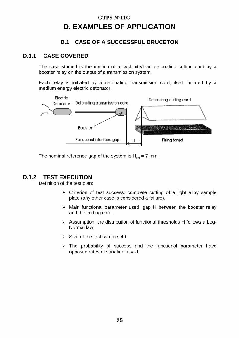
D.1.1 CASE COVERED

The case studied is the ignition of a cyclonite/lead detonating cutting cord by a booster relay on the output of a transmission system.

Each relay is initiated by a detonating transmission cord, itself initiated by a medium energy electric detonator.

The nominal reference gap of the system is HRef = 7 mm.

D.1.2 TEST EXECUTION Definition of the test plan:

� Criterion of test success: complete cutting of a light alloy sample plate (any other case is considered a failure),

� Main functional parameter used: gap H between the booster relay and the cutting cord,

� Assumption: the distribution of functional thresholds H follows a Log-Normal law,

� Size of the test sample: 40

� The probability of success and the functional parameter have opposite rates of variation: ε = -1.

GTPS N°11C

26

Procedure:

� Change of variable: X = Log10(H)

� hi: gap between relay and cord (in mm) at test level i

� xi = Log10(hi): operating level assigned to rank i (dimensionless variable)

� d: operating test pitch (d = xi – xi-1)

� ni: number of tests done at rank i

� N: total number of tests done (N ≤ 40)

� ε = -1

Performing the test sequence:

� Preliminary tests (N°1 ’ to 5 ') were made to conv erge towards the closed sequence (which begins in Test N°1 below)

� 3 preliminary tests (N°3 ', 4 ' and 5 ') were reus ed in the closed sequence (respectively for tests N°10, 5 and 2)

� The test sequence was conducted following the method and recommendations described in paragraph C.2.

� Testing stopped when a closed sequence of 32 tests was obtained..

1 2 3 4 5 6 7 8 9 10 11 12 13 14 15 16 17 18 19 20 21 22 23 24 25 26 27 28 29 30 31 32 33

5' 4' 3'

12.59 1.10 0 0 0 0 0 0 ?11.22 1.05 x x 0 0 0 0 0 0 0 x x x 0 x 0 x10.00 1.00 x x x 0 x x x x x x x8.91 0.95 x x7.94 0.90 x7.08 0.85 x

Closed sequence

3' 4' 5'hi (mm)

Xi =

Log( h i)1' 2'

Test N°33 has not been achieved: it is indicated on the diagram to show it is at the same level that Test N°1 of the closed sequence.

GTPS N°11C

27

D.1.3 USING TEST RESULTS

Use of closed sequence tests results in the following table:

h i (mm) x i i (ε = -1) n i n i*i i n i*i² i

12.59 1.10 0 6 0 0 11.22 1.05 1 15 15 15 10.00 1.00 2 10 20 40 8.91 0.95 3 1 3 9

32 38 64 Totals NS A B

NOTE: Since ε = -1, rank i=0 is assigned to the maximum level xM = 1.10 (or hM = 12.59 mm)

Evaluation of the mean:

� The estimator of the mean is equal to: 041.1/ =−= SM NdAxX

� Resulting in a mean of: mmH X 99.1010 ==

Evaluation of standard deviation:

� We calculate 3625.041

2 2

2

=

−−

−=

S

S

S

S

N

ABN

N

NU

� ϕ(U,Θ) is therefore determined for: 0.3 < U < 0.4

� We calculate the ratio A/NS = 1.1875, for which we take the fractional part to calculate Θ: Θ = 0.1875 = 3/16

� For Θ=3/16 and U=0.3625, the chart in Appendix 2 gives: ( ) 359.0, =ΘΦ Ue

� Then we calculate the estimator of standard deviation:

( ) 03052.0,7.1 =ΘΦ= Uds e

Validity check of the test:

� The test validity is checked by: 0.5 < d/s=1.64 < 2

Confidence interval on the mean (1-α = 90%):

� Using the table of normal distribution in Appendix 3, we determine the fractile uα/2 for a confidence level of 1-α = 90% (α/2=0.05): uα/2 = 1.645

� The mean variance can then be calculated: 52 10.4798.9

7.12

)3.1()( −==SN

sdXVar , giving a standard deviation of 0.0097365

� We deduce the bounds of the interval at 90% confidence on the mean:

+− =+=≤≤=−= mXVaruXmXVaruXm )(0566.10246.1)( 2/2/ αα

GTPS N°11C

28

Confidence interval on the standard deviation (1-α = 90%):

� We calculate 4.1429.0 =SN , allowing us to determine the number of degrees of

freedom (closest integer): ν= 14

� Using the Chi-Square table in Appendix 4, we determine the following values: 57.62

)2/,( =ανχ And 68.232)2/1,( =−ανχ

� We deduce the bounds of the interval at 90% confidence on the standard deviation:

+−

− ==≤≤== σχ

νσχ

νσαναν

2)2/,(

2)2/1,(

065.0018.0ss

Calculation of confidence level reliability (1-α/2)² = 90%:

� The reference level chosen is HRef = 7 mm.

� Resulting in a level Xref = Log10(HRef) = Log10(7) = 0.845,

� Reference level used for calculating reliability (increase of 10% - refer to recommendation Nº3 at C3): 1.1xXRef = 0.9295

� We then calculate the reliability: 928.0065.0

9295.00246.1 =

−=

−=

+

− FXm

FR Réf

σ

NOTE: Without using recommendation Nº3 of C3, the reliability calculated at reference level 0.845 would have been 0.997.

D.2 CASE OF A SUCCESSFUL BRUCETON WITH PITCH ADJUST MENT

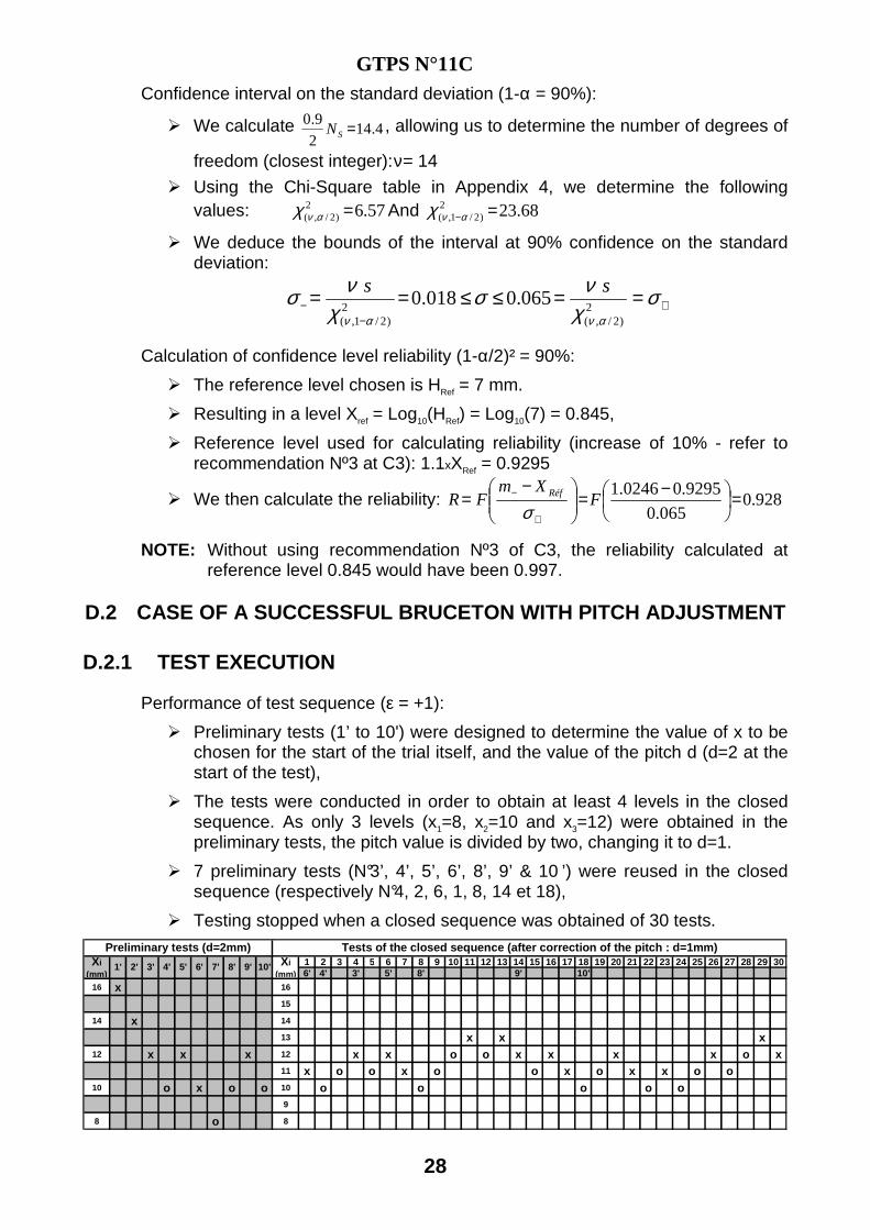
D.2.1 TEST EXECUTION

Performance of test sequence (ε = +1):

� Preliminary tests (1’ to 10') were designed to determine the value of x to be chosen for the start of the trial itself, and the value of the pitch d (d=2 at the start of the test),

� The tests were conducted in order to obtain at least 4 levels in the closed sequence. As only 3 levels (x1=8, x2=10 and x3=12) were obtained in the preliminary tests, the pitch value is divided by two, changing it to d=1.

� 7 preliminary tests (N°3’, 4’, 5’, 6’, 8’, 9’ & 10 ’) were reused in the closed sequence (respectively N°4, 2, 6, 1, 8, 14 et 18),

� Testing stopped when a closed sequence was obtained of 30 tests.

1 2 3 4 5 6 7 8 9 10 11 12 13 14 15 16 17 18 19 20 21 22 23 24 25 26 27 28 29 306' 4' 3' 5' 8' 9' 10'

16 x 16

15

14 x 14

13 x x x12 x x x 12 x x o o x x x x o x

11 x o o x o o x o x x o o10 o x o o 10 o o o o o

9

8 o 8

Preliminary tests (d=2mm) Tests of the closed sequen ce (after correction of the pitch : d=1mm)Xi

(mm)1' 2' 3' 4' 5' 6' Xi

(mm)7' 8' 9' 10'

GTPS N°11C

29

D.2.2 USING TEST RESULTS

Use of closed sequence tests gives the following table:

x i i (ε = +1) n i n i*i n i*i²

13 3 3 9 27 12 2 10 20 40 11 1 12 12 12 10 0 5 0 0

30 41 79 Totals NS A B

NOTE: Since ε = +1, the rank i=0 is attributed to the minimum level xm = 9.

Evaluation of the mean:

� The estimator of the mean is equal to: 37.11/ =+= Sm NdAxX

Evaluation of standard deviation:

� Calculate 5524.041

2 2

2

=

−−

−=

S

S

S

S

N

ABN

N

NU

� ϕ(U,Θ) is therefore determined for: U > 0.4

� Therefore Φe(U,Θ) = U = 0.5524

� Then calculate the estimator of standard deviation: ( ) 939.0,7.1 =ΘΦ= Uds e

Validity check of the test:

� The test validity is checked by: 0.5 < d/s=1.064 < 2

Confidence interval on the mean (1-α = 90%):

� Using the table of normal distribution in Appendix 3, we determine the fractile uα/2 for a confidence level of 1-α = 90% (α/2=0.05): uα/2 = 1.645

� The variance of the mean can be calculated: 22 10.62.67.12

)3.1()( −==SN

sdXVar ,

giving a standard deviation of 0.2495

� We deduce the bounds of the interval at 90% confidence on the mean:

+− =+=≤≤=−= mXVaruXmXVaruXm )(778.11956.10)( 2/2/ αα

GTPS N°11C

30

Confidence interval for standard deviation (1-α = 90%):

� We calculate 5.1329.0 =SN , allowing us to determine the number of degrees of

freedom (nearest integer number): ν= 14,

� Using the Chi-Square table in Appendix 4, we determine the following values: 57.62

)2/,( =ανχ and 68.232)2/1,( =−ανχ

� We deduce the bounds of the interval at 90% confidence on the standard deviation:

+−

− ==≤≤== σχ

νσχ

νσαναν

2)2/,(

2)2/1,(

0008.25551.0ss

Calculation of a functional threshold at the confidence level (1-α/2)² = 90%:

� The desired reliability level is R = 0.999, � Then calculate the functional threshold:

( ) mmRFmRX F 96.17)()2/1(, 12 =+=− +−

+ σα

� The functional threshold level used after increasing by 10% (See recommendation Nº3 at §C3): ( ) mmRX F 76.19)2/1(,1,1 2 =−× α .

NOTE: Without using recommendation Nº3 of §C3, the reliability calculated at the functional threshold used of 19.76mm would be 0.999967.

D.3 CASE OF A DISPERSED BRUCETON (NOT USABLE)

During a Bruceton test, we obtained the following closed sequence (ε = -1):

1 2 3 4 5 6 7 8 9 10 11 12 13 14 15 16 17 18 19 20 21 22 23 24 25 26 27 28 29 30 31 32 33 34

13 0 012 0 x 0 0 0 x 011 x 0 0 x x x 0 x 010 x x 0 0 0 x x9 0 x x 0 x8 x 0 x7 x

Xi

(mm)Closed sequence

Use of closed sequence tests gives the following table:

x i i (ε = -1) n i n i*i n i*i²

13 0 2 0 0 12 1 7 7 7 11 2 9 18 36 10 3 7 21 63 9 4 5 20 80 8 5 3 15 75 7 6 1 6 36

34 87 297 Totals NS A B

GTPS N°11C

31

Evaluation of the mean:

� The estimator of the mean is equal to: 44.10/ =−= SM NdAxX

Evaluation of standard deviation:

� Calculate 0588.241

2 2

2

=

−−

−=

S

S

S

S

N

ABN

N

NU

� ϕ(U,Θ) is therefore determined for: U > 0.4

� Therefore Φe(U,Θ) = U = 2.0588

� Then calculate the estimator of standard deviation: ( ) 5.3,7.1 =ΘΦ= Uds e

Validity check of the test:

� The test validity criteria is not met: d/s=0.29 < 0.5

Therefore, this Bruceton test cannot be used.

NOTE: The result of test 24 induces 7 levels in the usable sequence, and it would have been appropriate at this time to correct the pitch value before continuing the tests and their use (See recommendation Nº1 at §C3).

E. CONCLUSION

This recommendation outlines the procedure for using the Bruceton method applicable to the evaluation of a probability of success or failure, during the operation of a one-shot device at a given reference level.

It relies on using the "Saubade" method, for which a mathematical justification now exists (refer to 35 in appendix 6).

This method makes explicit the approach to be followed (implementation conditions strictly speaking) with particular emphasis on:

� Determination of test levels,

� Conduct of these tests.

It assumes that the probability distribution law of functional thresholds of the functional parameter used follows a normal distribution law (or a Log-Normal, by changing a variable).

It can be used to evaluate the estimators of the mean and standard deviation from a sample consisting of at least 30 specimens.

Evaluation of these estimators, associated with a given confidence level, can be used to evaluate the probability of successful operation of a one-shot device under the effect of a defined stimulus level.

GTPS N°11C

32

This recommendation gives operating limits not to be exceeded through examples of applications in Bruceton tests:

� Successful,

� Successful with pitch adjustment,

� Deemed unusable.

This method integrates into the general approach of reliability study (or safety study) of a pyrotechnic system.

It is applied during the design phase of a product (pre-project, development).

It may also be applicable to the phases of mass production, use and dismantling of the product.

GTPS N°11C

33

APPENDIX 1: VERIFICATION OF REPRESENTATIVENESS OF S AMPLES TESTED

Note: The specimen includes the product and its means of testing if it is consumable (e.g. targets for explosives).

What is the permitted capability for this means of manufacture for the

tolerance requested:extraction of mean and standard

deviation

is the technology used planned for mass production?

Manufacture and Inspection of test specimens

Estimate of risk that the specimens manufactured will not belong to the

mass production population

Is the risk acceptable?

Start again with new test specimens

no

yes

yes

Is the risk acceptable?

Manufacture of test specimens using another known and

controlled means

no

no

no

yes

yes

Production Meanstest specimens

Specimens manufactured are usable for tests

use of feedback from prior

similar projects

Flowchart input

Is there feedback on the

technology used?

What is the permitted capability for this means of manufacture for the

tolerance requested:extraction of mean and standard

deviation

is the technology used planned for mass production?

Manufacture and Inspection of test specimens

Estimate of risk that the specimens manufactured will not belong to the

mass production population

Is the risk acceptable?

Start again with new test specimens

no

yes

yes

Is the risk acceptable?

Manufacture of test specimens using another known and

controlled means

no

no

no

yes

yes

Production Meanstest specimens

Specimens manufactured are usable for tests

use of feedback from prior

similar projects

Flowchart input

Is there feedback on the

technology used?

G

TP

S N

°11C

34

AP

PE

ND

IX 2: C

HA

RT

ΦΦΦ ΦE (U

,ΘΘΘ Θ)

0

1/6 1/8

3/16 1/4

5/16 3/8

7/16 1/2

ΘΘΘ Θ

0 0.1667

0.125 0.1875

0.25 0.3125

0.375 0.4375

0.5

0.28

0.29

0.3

0.31

0.32

0.33

0.34

0.35

0.36

0.37

0.38

0.39

0.4

0.41

0.3 0.31 0.32 0.33 0.34 0.35 0.36 0.37 0.38 0.39 0.4

Θ=0Θ=1/16Θ=1/8Θ=3/16Θ=1/4Θ=5/16Θ=3/8Θ=7/16Θ=1/2

ΦΦΦΦe(U,ΘΘΘΘ)

U

Θ Θ Θ Θ = = = = 1111////2222

Θ Θ Θ Θ = = = = 0000

GTPS N°11C

35

APPENDIX 3: TABLE OF STANDARD NORMAL DISTRIBUTION Overlooking the value of the fractile uα/2 depending of α/2

αααα/2/2/2/2 0.000 0.001 0.002 0.003 0.004 0.005 0.006 0.007 0.008 0.009 0.01

0.00 3.090 2.878 2.748 2.652 2.576 2.512 2.457 2.409 2.366 2.326 0.01 2.326 2.290 2.257 2.226 2.197 2.170 2.144 2.120 2.097 2.075 2.054 0.02 2.054 2.034 2.014 1.995 1.977 1.960 1.943 1.927 1.911 1.896 1.881 0.03 1.881 1.866 1.852 1.838 1.825 1.812 1.799 1.787 1.774 1.762 1.751 0.04 1.751 1.739 1.728 1.717 1.706 1.695 1.685 1.675 1.665 1.655 1.645 0.05 1.645 1.635 1.626 1.616 1.607 1.598 1.589 1.580 1.572 1.563 1.555 0.06 1.555 1.546 1.538 1.530 1.522 1.514 1.506 1.499 1.491 1.483 1.476 0.07 1.476 1.468 1.461 1.454 1.447 1.440 1.433 1.426 1.419 1.412 1.405 0.08 1.405 1.398 1.392 1.385 1.379 1.372 1.366 1.359 1.353 1.347 1.341 0.09 1.341 1.335 1.329 1.323 1.317 1.311 1.305 1.299 1.293 1.287 1.282 0.1 1.282 1.276 1.270 1.265 1.259 1.254 1.248 1.243 1.237 1.232 1.227

0.11 1.227 1.221 1.216 1.211 1.206 1.200 1.195 1.190 1.185 1.180 1.175 0.12 1.175 1.170 1.165 1.160 1.155 1.150 1.146 1.141 1.136 1.131 1.126 0.13 1.126 1.122 1.117 1.112 1.108 1.103 1.098 1.094 1.089 1.085 1.080 0.14 1.080 1.076 1.071 1.067 1.063 1.058 1.054 1.049 1.045 1.041 1.036 0.15 1.036 1.032 1.028 1.024 1.019 1.015 1.011 1.007 1.003 0.999 0.994 0.16 0.994 0.990 0.986 0.982 0.978 0.974 0.970 0.966 0.962 0.958 0.954 0.17 0.954 0.950 0.946 0.942 0.938 0.935 0.931 0.927 0.923 0.919 0.915 0.18 0.915 0.912 0.908 0.904 0.900 0.896 0.893 0.889 0.885 0.882 0.878 0.19 0.878 0.874 0.871 0.867 0.863 0.860 0.856 0.852 0.849 0.845 0.842 0.2 0.842 0.838 0.834 0.831 0.827 0.824 0.820 0.817 0.813 0.810 0.806

0.21 0.806 0.803 0.800 0.796 0.793 0.789 0.786 0.782 0.779 0.776 0.772 0.22 0.772 0.769 0.765 0.762 0.759 0.755 0.752 0.749 0.745 0.742 0.739 0.23 0.739 0.736 0.732 0.729 0.726 0.722 0.719 0.716 0.713 0.710 0.706 0.24 0.706 0.703 0.700 0.697 0.693 0.690 0.687 0.684 0.681 0.678 0.674 0.25 0.674 0.671 0.668 0.665 0.662 0.659 0.656 0.653 0.650 0.646 0.643 0.26 0.643 0.640 0.637 0.634 0.631 0.628 0.625 0.622 0.619 0.616 0.613 0.27 0.613 0.610 0.607 0.604 0.601 0.598 0.595 0.592 0.589 0.586 0.583 0.28 0.583 0.580 0.577 0.574 0.571 0.568 0.565 0.562 0.559 0.556 0.553 0.29 0.553 0.550 0.548 0.545 0.542 0.539 0.536 0.533 0.530 0.527 0.524 0.3 0.524 0.522 0.519 0.516 0.513 0.510 0.507 0.504 0.502 0.499 0.496

0.31 0.496 0.493 0.490 0.487 0.485 0.482 0.479 0.476 0.473 0.470 0.468 0.32 0.468 0.465 0.462 0.459 0.457 0.454 0.451 0.448 0.445 0.443 0.440 0.33 0.440 0.437 0.434 0.432 0.429 0.426 0.423 0.421 0.418 0.415 0.412 0.34 0.412 0.410 0.407 0.404 0.402 0.399 0.396 0.393 0.391 0.388 0.385 0.35 0.385 0.383 0.380 0.377 0.375 0.372 0.369 0.366 0.364 0.361 0.358 0.36 0.358 0.356 0.353 0.350 0.348 0.345 0.342 0.340 0.337 0.335 0.332 0.37 0.332 0.329 0.327 0.324 0.321 0.319 0.316 0.313 0.311 0.308 0.305 0.38 0.305 0.303 0.300 0.298 0.295 0.292 0.290 0.287 0.285 0.282 0.279 0.39 0.279 0.277 0.274 0.272 0.269 0.266 0.264 0.261 0.259 0.256 0.253 0.4 0.253 0.251 0.248 0.246 0.243 0.240 0.238 0.235 0.233 0.230 0.228

0.41 0.228 0.225 0.222 0.220 0.217 0.215 0.212 0.210 0.207 0.204 0.202 0.42 0.202 0.199 0.197 0.194 0.192 0.189 0.187 0.184 0.181 0.179 0.176 0.43 0.176 0.174 0.171 0.169 0.166 0.164 0.161 0.159 0.156 0.154 0.151 0.44 0.151 0.148 0.146 0.143 0.141 0.138 0.136 0.133 0.131 0.128 0.126 0.45 0.126 0.123 0.121 0.118 0.116 0.113 0.111 0.108 0.105 0.103 0.100 0.46 0.100 0.098 0.095 0.093 0.090 0.088 0.085 0.083 0.080 0.078 0.075 0.47 0.075 0.073 0.070 0.068 0.065 0.063 0.060 0.058 0.055 0.053 0.050 0.48 0.050 0.048 0.045 0.043 0.040 0.038 0.035 0.033 0.030 0.028 0.025 0.49 0.025 0.023 0.020 0.018 0.015 0.013 0.010 0.008 0.005 0.003 0.000

Example: If 1-α=90%, α/2 = 0.05: reads Uα/2 = 1.645 at the intersection of "0.05" line and

« 0.000 » column Remark: It is recommended to use confidence levels between 0.9 and 0.95.

GTPS N°11C

36

APPENDIX 4: TABLE OF PEARSON CHI-SQUARE DISTRIBUTIO N Overlooking the value of 2

)2/,( ανχ depending on αααα/2/2/2/2 and the number of degrees of freedom νννν

αααα/2 νννν 0.995 0.990 0.950 0.900 0.800 0.700 0.600 0.500 0.400 0.300 0.200 0.100 0.050 0.010 0.005

1 7.88 6.63 3.84 2.71 1.64 1.07 0.71 0.45 0.27 0.15 0.064 0.016 0.004 0.0002 0.00004 2 10.60 9.21 5.99 4.61 3.22 2.41 1.83 1.39 1.02 0.71 0.446 0.211 0.103 0.020 0.010 3 12.84 11.34 7.81 6.25 4.64 3.66 2.95 2.37 1.87 1.42 1.01 0.58 0.35 0.11 0.07 4 14.86 13.28 9.49 7.78 5.99 4.88 4.04 3.36 2.75 2.19 1.65 1.06 0.71 0.30 0.21 5 16.75 15.09 11.07 9.24 7.29 6.06 5.13 4.35 3.66 3.00 2.34 1.61 1.15 0.55 0.41 6 18.55 16.81 12.59 10.64 8.56 7.23 6.21 5.35 4.57 3.83 3.07 2.20 1.64 0.87 0.68 7 20.28 18.48 14.07 12.02 9.80 8.38 7.28 6.35 5.49 4.67 3.82 2.83 2.17 1.24 0.99 8 21.95 20.09 15.51 13.36 11.03 9.52 8.35 7.34 6.42 5.53 4.59 3.49 2.73 1.65 1.34 9 23.59 21.67 16.92 14.68 12.24 10.66 9.41 8.34 7.36 6.39 5.38 4.17 3.33 2.09 1.73 10 25.19 23.21 18.31 15.99 13.44 11.78 10.47 9.34 8.30 7.27 6.18 4.87 3.94 2.56 2.16

11 26.76 24.72 19.68 17.28 14.63 12.90 11.53 10.34 9.24 8.15 6.99 5.58 4.57 3.05 2.60 12 28.30 26.22 21.03 18.55 15.81 14.01 12.58 11.34 10.18 9.03 7.81 6.30 5.23 3.57 3.07 13 29.82 27.69 22.36 19.81 16.98 15.12 13.64 12.34 11.13 9.93 8.63 7.04 5.89 4.11 3.57 14 31.32 29.14 23.68 21.06 18.15 16.22 14.69 13.34 12.08 10.82 9.47 7.79 6.57 4.66 4.07 15 32.80 30.58 25.00 22.31 19.31 17.32 15.73 14.34 13.03 11.72 10.31 8.55 7.26 5.23 4.60 16 34.27 32.00 26.30 23.54 20.47 18.42 16.78 15.34 13.98 12.62 11.15 9.31 7.96 5.81 5.14 17 35.72 33.41 27.59 24.77 21.61 19.51 17.82 16.34 14.94 13.53 12.00 10.09 8.67 6.41 5.70 18 37.16 34.81 28.87 25.99 22.76 20.60 18.87 17.34 15.89 14.44 12.86 10.86 9.39 7.01 6.26 19 38.58 36.19 30.14 27.20 23.90 21.69 19.91 18.34 16.85 15.35 13.72 11.65 10.12 7.63 6.84 20 40.00 37.57 31.41 28.41 25.04 22.77 20.95 19.34 17.81 16.27 14.58 12.44 10.85 8.26 7.43

21 41.40 38.93 32.67 29.62 26.17 23.86 21.99 20.34 18.77 17.18 15.44 13.24 11.59 8.90 8.03 22 42.80 40.29 33.92 30.81 27.30 24.94 23.03 21.34 19.73 18.10 16.31 14.04 12.34 9.54 8.64 23 44.18 41.64 35.17 32.01 28.43 26.02 24.07 22.34 20.69 19.02 17.19 14.85 13.09 10.20 9.26 24 45.56 42.98 36.42 33.20 29.55 27.10 25.11 23.34 21.65 19.94 18.06 15.66 13.85 10.86 9.89 25 46.93 44.31 37.65 34.38 30.68 28.17 26.14 24.34 22.62 20.87 18.94 16.47 14.61 11.52 10.52 26 48.29 45.64 38.89 35.56 31.79 29.25 27.18 25.34 23.58 21.79 19.82 17.29 15.38 12.20 11.16 27 49.64 46.96 40.11 36.74 32.91 30.32 28.21 26.34 24.54 22.72 20.70 18.11 16.15 12.88 11.81 28 50.99 48.28 41.34 37.92 34.03 31.39 29.25 27.34 25.51 23.65 21.59 18.94 16.93 13.56 12.46 29 52.34 49.59 42.56 39.09 35.14 32.46 30.28 28.34 26.48 24.58 22.48 19.77 17.71 14.26 13.12 30 53.67 50.89 43.77 40.26 36.25 33.53 31.32 29.34 27.44 25.51 23.36 20.60 18.49 14.95 13.79

31 55.00 52.19 44.99 41.42 37.36 34.60 32.35 30.34 28.41 26.44 24.26 21.43 19.28 15.66 14.46 32 56.33 53.49 46.19 42.58 38.47 35.66 33.38 31.34 29.38 27.37 25.15 22.27 20.07 16.36 15.13 33 57.65 54.78 47.40 43.75 39.57 36.73 34.41 32.34 30.34 28.31 26.04 23.11 20.87 17.07 15.82 34 58.96 56.06 48.60 44.90 40.68 37.80 35.44 33.34 31.31 29.24 26.94 23.95 21.66 17.79 16.50 35 60.27 57.34 49.80 46.06 41.78 38.86 36.47 34.34 32.28 30.18 27.84 24.80 22.47 18.51 17.19 36 61.58 58.62 51.00 47.21 42.88 39.92 37.50 35.34 33.25 31.12 28.73 25.64 23.27 19.23 17.89 37 62.88 59.89 52.19 48.36 43.98 40.98 38.53 36.34 34.22 32.05 29.64 26.49 24.07 19.96 18.59 38 64.18 61.16 53.38 49.51 45.08 42.05 39.56 37.34 35.19 32.99 30.54 27.34 24.88 20.69 19.29 39 65.48 62.43 54.57 50.66 46.17 43.11 40.59 38.34 36.16 33.93 31.44 28.20 25.70 21.43 20.00 40 66.77 63.69 55.76 51.81 47.27 44.16 41.62 39.34 37.13 34.87 32.34 29.05 26.51 22.16 20.71

41 68.05 64.95 56.94 52.95 48.36 45.22 42.65 40.34 38.11 35.81 33.25 29.91 27.33 22.91 21.42 42 69.34 66.21 58.12 54.09 49.46 46.28 43.68 41.34 39.08 36.75 34.16 30.77 28.14 23.65 22.14 43 70.62 67.46 59.30 55.23 50.55 47.34 44.71 42.34 40.05 37.70 35.07 31.63 28.96 24.40 22.86 44 71.89 68.71 60.48 56.37 51.64 48.40 45.73 43.34 41.02 38.64 35.97 32.49 29.79 25.15 23.58 45 73.17 69.96 61.66 57.51 52.73 49.45 46.76 44.34 42.00 39.58 36.88 33.35 30.61 25.90 24.31 46 74.44 71.20 62.83 58.64 53.82 50.51 47.79 45.34 42.97 40.53 37.80 34.22 31.44 26.66 25.04 47 75.70 72.44 64.00 59.77 54.91 51.56 48.81 46.34 43.94 41.47 38.71 35.08 32.27 27.42 25.77 48 76.97 73.68 65.17 60.91 55.99 52.62 49.84 47.34 44.92 42.42 39.62 35.95 33.10 28.18 26.51 49 78.23 74.92 66.34 62.04 57.08 53.67 50.87 48.33 45.89 43.37 40.53 36.82 33.93 28.94 27.25 50 79.49 76.15 67.50 63.17 58.16 54.72 51.89 49.33 46.86 44.31 41.45 37.69 34.76 29.71 27.99

Example: If 1-αααα=90% and if νννν = 14 degrees of freedom: � α/2 = 0.05 and reads 2

)2/,( ανχ = 6.57 at the intersection of "0.05" column

and « 14 » line. � 1-α/2 = 0.95 and reads 2

)2/1,( ανχ − = 23.68 at the intersection of "0.95"

column and « 14 » line. Remark: It is recommended to use confidence levels between 0.9 and 0.95.

GTPS N°11C

37

APPENDIX 5: RECAP SUMMARY

Normal or Log-Normal distribution law:

If the probability law of the functional parameter studied is Log-Normal, the following principles are applied:

� H: functional parameter studied, and hi the test levels of this parameter,

� Change of variable: o X = Log10 (H): transformed variable is dimensionless, o Xi = Log10 (hi): levels of exploitation of this parameter.

Direction of variation:

If the probability law of success and functional parameter studied are:

� In the same direction of variation: ε = +1,

� In opposite directions of variation: ε = -1.

Statistical estimators:

Estimator of the mean x :

� Sm NdAXx /+= if ε = +1,

� SM NdAXx /−= if ε = -1.

Estimator of the standard deviation s:

� s = 1.7dΦe(U,Θ) if 0.3 ≤U < 0.4,

� s= 1.7dU if U ≥ 0.4,

� Test unusable without adjusting the pitch if U < 0.3

Confidence intervals at level (1- αααα):

Confidence interval on the mean m:

� +− =+≤≤−= mxVaruxmxVaruxm )()( 2/2/ αα with:

o SN

sd

s

dxVar

7.1

218.03.1)(

2

−+= for 0.5 ≤ d/s ≤ 1

o [ ]SN

sdxVar

7.1

23.1)( 2= for 1 ≤ d/s ≤ 2

Confidence interval on the standard deviation σ:

� +−

− =≤≤= σχ

νσχ

νσαναν

2)2/,(

2)2/1,(

ss

o With SN2

9.0=ν (ν is an integer)

GTPS N°11C

38

Evaluation of reliability at confidence level (1- αααα/2)²:

If Xref > m+

� ( ) ( )

−==−

+

+

σα

mXFuFXR Réf

XRéf Réf

2)2/1(,

� ( ) ( ) +

−+ +=−=− σαα )()2/1(,)2/1(, 122 RFmRXRX NFF

If Xref < m-:

� ( ) ( )

−==−

+

−

σα Réf

XRéf

XmFuFXR

Réf

2)2/1(,

� ( ) ( ) +

−− −=−=− σαα )()2/1(,)2/1(, 122 RFmRXRX NFF

GTPS N°11C

39

APPENDIX 6: BIBLIOGRAPHY ON THE BRUCETON METHOD

1. BASTENAIRE F. - REGNIER L.

"Etude des propriétés statistiques des estimateurs des paramètres d'une courbe de réponse obtenue par la méthode de l'escalier" Revue de statistique appliquée. vol. 31. pages 5 to 24 (1983).

2. BAUER R.J. - AYRES J.N.

"A method for estimating the upper Iîmit of the variability parameter in two and three levels symetrieal Bruceton tests" Naval Surface Weapons Center White Oak Lab., Silver SprÎl1g, Final report 75-77,35 pages. Contract MIPR-2311-BO 33 (20/10/80) ou M.Report WONSWCNVOLITR-77-134.

3. BOWKER AH. - LlEBERMAN G.J.

"Méthodes statistiques de l'ingénieur" DUNOD (1965).

4. BROWNLEE KA - HODGES J.L. - ROSENBLATT M.

"The up and down method with small samples" Journal of the American Statistical Association, vol. 48, pages 262 to 277 (1953).

5. CULLING H.P. (*)

"Statistical methods appropriate for evaluation of fuze explosive train safety and reliability" US NOL, White Oak. Navord Report 2101, AD 066-428 (10/53).

6. DESROCHES A.

"Quelques modèles statistiques non classiques utilisables dans les tests de sensibilité" Revue de statistique appliquée, vol. 30, (3), pages15 to 25 (1982).

7. DIXON W.J. - MOOD AM. (*)

"A method for obtaining and analysing sensitivity data" American Statistical Association Journal, vol. 43, pages 109 to 126 (1948).

8. DIXON W.J. - MOOD AM. (*)

"Introduction to statistical analysis" McGRAW-HILL Book Company. INC, second edition (1957).

9. DIXON W.J. (*)

"The up and down method for small samples" American Statistical Association Journal, vol. 60, pages 967 to 978 (12/1965).

10. EFAB

"Exploitation statistique de tests de sensibilité - Méthode logistique logarithmique". Etablissement d'études et de fabrications d'armement de Bourges. Note documentaire.

11. GRANT R.L. - VAN DOLAH R-W.

"Use of the up and down method with factorial designs" US Army Research Office, Box CM, Duke Station, Durham, North Carolina. ARODR 62-2. Proceedings of the seventh Conference of the design of experiments in Army research development and testing, pages 39 to 65 (1964).

12. G.T.P.S. (*)

"Méthodes statistiques - Méthode de Bruceton" Doc N°11C (09/82).

GTPS N°11C

40

13. G.T.P.S. (*)

"Méthodes statistiques - Méthode de Bruceton - Application aux faibles échantillons" Doc W11 D (09/89).

14. HAMPTON L.D. "Monte Carlo investigations on small sample Bruceton tests"

US NOL, White Oak. Navord Report 66, AD 117-649 (255/17).

15. HAMPTON L.D. - BLUM G.D. - AYRES J.N. "Logistical analysis of Bruceton data" US NOL. White Oak. NOLTR 73-91, AD 766-780 (23/07/73).

16. de JONCKERE R. (*)

"Les essais de sensibilité par la méthode up and down" Service Technique De La Force Terrestre. Revue X - Tijdschrift N° 2 (1975).

17. LANIER E. – THIVET R.

"Méthode Bruceton et programme de calcul" (Annexe 3, NT 118/80/CRB/NP). NT 25/81/CRB/NP : "Seuil de sensibilité à un choc standard"

18. LAURENT M.

"Utilisation pratique de la méthode séquentielle de Bruceton en variable logarithmique" Etablissement Technique de Bourges. ETBS/CT/N° 139/ Cds176 (26/10/76).

19. LEJUEZ W. (*)

"Méthode de Bruceton - Application aux faibles échantillons" SEP Etudes générales de fiabilité. Note GT/M 938290 (10/02/89).

20. LEJUEZ W. (*)

"Méthode de Bruceton - Etude théorique dans le cas d'une sollicitation appliquée avec ou sans incertitude" SEP. Etudes générales de fiabilité TP 29631/83. marché DTEN 115/1983 (25/01/84).

21. LEJUEZ W. (*)

"Nouvelle approche de l'exploitation du test de Bruceton" SEP. 5ème colloque international de fiabilité et de maintenabilité, Biarritz (1986).

22. LEJUEZ W. (*)

"Méthode de Bruceton - Dépouillement du test dans le cas de sollicitations appliquées avec ou sans incertitude" SEP. Etudes générales de fiabilité TP 431077 WL/yn, marché DTEN 115/1983 (19/03/84).

23. MALABIAU R (*)

"Méthodes statistiques utilisables pour déterminer la sensibilité des dispositifs électro-pyrotechniques à diverses excitations d’origine électrique ou électromagnétique". Groupe d'Etude et Recherche de Pyrotechnie, DCAN Toulon. Colloque "Explosifs et pyrotechnie" en Applications spatiales, Toulouse (23-25/10/79). CNES/ESA SP 144, pages 179 to 200 (01/80).

24. MALABIAU R.

"Tests statistiques utilisables en électro-pyrotechnie" Groupe d'Etude et Recherche de Pyrotechnie, DCAN Toulon.

GTPS N°11C

41

25. MARTIN J.W. - SAUNDERS J. "Bruceton tests - Results of a computer study an small sample accuracy” Procedings of electrIc Symposium, AD 4407 64 (1963) or International conference on sensitivity and hazards of explosives, London (1-3/10/63) or Note TBA (25/06/70)

26. NASA (*)

"A guide for the application of the Bruceton method to electro explosive devices" NASA-MSC. N70-35807 (09/66).

27. NOL

"Comparison of the Probit method and the Bruceton up and down method as applied to sensitivity data" US NOL, White Oak. NOLM 9910, AD 106-866 (11/48).

28. PECKHAM H. (*)

"Flow chart for Bruceton analysis" Holex Incorporated, rev. A, San Juan Road, Hollistor, California. Mercury 7-5306.

29. PFEFFER G. (*)

"Degré de confiance de l'évaluation de la fiabilité en sécurité ou en sûreté d'une chaine pyrotechnique" Thomson Armement. Colloque sur les applications modernes de la pyrotechnie, Toulon, pages 77 to 105 (19-22/06/73).

30. PINON I.G. (*)

"Exploitation statistique de tests de sensibilité - Emploi pratique de la méthode séquentielle de Bruceton" Etablissement d'Etudes et de Fabrication d'Armement de Bourges, Département Etudes Pyrotechnie. Note documentaire (1969).

31. PINON I.G. (*)

"Note complémentaire sur les tests de sensibilité - Tests de Bruceton en variable logarithmique" Etablissement d'Etudes et de Fabrication d'Armement de Bourges, Département Etudes Pyrotechnie. Note documentaire W 29502 (03/07/69).

32. RASPAUD L. (*)

"Essais de sensibilité par les méthodes Bruceton et probits" Interface SA. (02/92). Commande 843/91/CNES6310 du 06/12/91.

33. RASPAUD L. - AUGER P. (*)

"Essais de sensibilité par les méthodes one-shor, Bruceton et probits" Interface SA. CNES NT-397/CT/AE/MT/2P (17/06/94).

34. RASPAUD L. (*)

"Essais de sensibilité" Interface SA (10/94). Commande 840/2/94/CNES/0115 of 19/09/94.

35. SAUBADE Ch. (*)

"Essais de sensibilité par la méthode Bruceton" Aérospatiale/Aquitaine. Note NT 12282/AQES/D (05/04/82).

36. STECKER E.J. (*)

"Bruceton test method" Holex Incorporated, rev. A, San Juan Road, Hollistor, California. Mercury 7-5306 or Note 47/71 GERPY (06/04/71).

GTPS N°11C

42

37. THOMSON BRANDT

"Proposition technique concernant la comparaison des efficacités des tests de Bruceton, one-shot et Probit" Note technique 23.110 : Etablissement de la fiabilité expérimentale d'éléments et systèmes monocoups.

38. G.T.P.S. (*)

"Méthodes statistiques - Méthode de Bruceton" Doc N°11C (09/98).

39. CNES (*)

"Comparaison expérimentale des méthodes One-Shot, Bruceton et Probits - DLA-NT-0-988-AP" Note de Synthèse de l'activité PAQTE 2004-DLA-05

40. CNES (*)

"Etude des méthodes de fiabilité en pyrotechnie - LIGERON (10/08)" Commande n°4700024528/DCT 094 of 29/05/08

(*) Note: Documents analysed in this study