bruker-microct method note: automated trabecular...
TRANSCRIPT
Page 1 of 18
Automated trabecular and
cortical bone selection
Method note

Page 2 of 18
2 Bruker-MicroCT method note: Automated trabecular and cortical bone selection
Introduction
In practice, quantitative analysis of long bone morphology is subdivided into analysis
of the trabecular bone and analysis of the cortical bone. To do so, one has to
adequately set a region of interest corresponding to either the trabecular bone or the
cortical bone. This is very time-consuming as it has to be done manually for every
individual bone.
The goal of this application note is to demonstrate how this can be done in an
automated way using custom processing, which is much faster and more accurate
than the manual way, increasing reproducibility of the results and lowering variation.
Part 1: Regions of interest (ROI) page
Before opening the dataset in CTAn, make sure the long axis of the bone is aligned
along the Z-axis. If not, one can reorient the dataset using dataviewer and save the
dataset in the right orientation. Upon opening of the dataset in CTAn, browse to the
‘Regions of interest’ page. The first and only manual step is to save 2 new
datasets: a subset of slices in the long bone metaphysis to run the trabecular
analysis (‘VOI trab’), and a subset of slices in the long bone diaphysis to run the
cortical analysis (‘VOI cort’). Typically, one will select the growth plate as a reference
point and define a specific offset and height to select the appropriate region
(described in detail in the method note ‘mouse bone analysis method’). Yet, and in
contrast to what used to be done, no specific ROI has to be created on the slices
themselves to separate the trabecular bone from the cortical bone.
Slice of metapyseal ROI Slice of diapyseal ROI
Page 3 of 18
3 Bruker-MicroCT method note: Automated trabecular and cortical bone selection
Part 2: Custom processing page
Starting from the ROI datasets that have been saved, one used to manually draw a
ROI separating the trabecular bone from the cortical bone in order not to contaminate
the trabecular analysis with (parts of the) cortical bone and the other way around.
However, using custom processing, it is possible to run an automated task list to do
so. First a protocol will be set up to automatically select the trabecular part of the
bone (the bone marrow cavity in principal), and a few more steps will be added to this
protocol in case a cortical selection is required.
A. Trabecular selection
After opening the ‘VOI trab’ dataset, one first has to browse to the binary page to
select an appropriate threshold to segment the bone from the soft tissue and
background. In this case, a threshold of 80 was selected. Once the correct threshold
values are selected, proceed to the ‘Custom processing’ page.
A copy of the dataset will be loaded. Three very important buttons are on the right
side of the plug-ins bar:
image view
image inside ROI view
ROI view
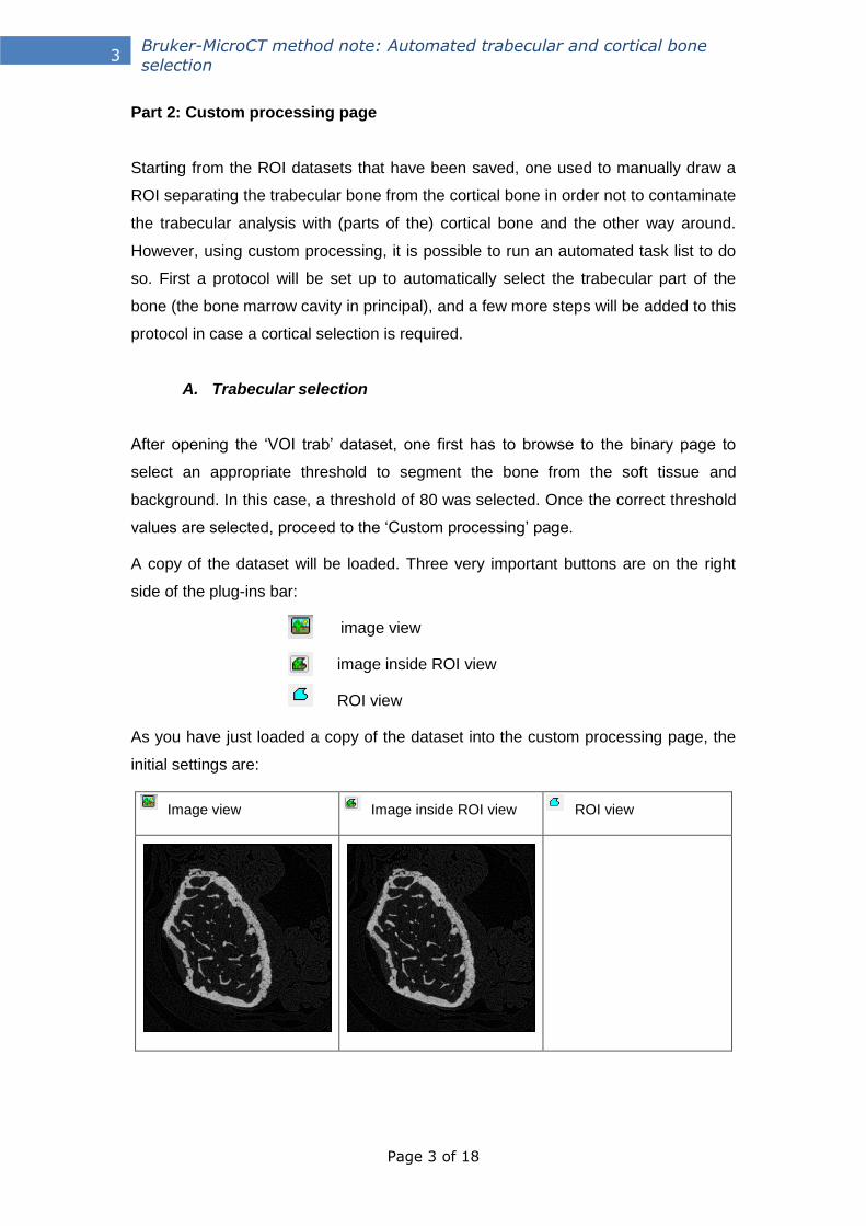
As you have just loaded a copy of the dataset into the custom processing page, the
initial settings are:
Image view Image inside ROI view ROI view

Page 4 of 18
4 Bruker-MicroCT method note: Automated trabecular and cortical bone selection
The idea behind an automated trabecular selection is in fact delineating the bone
marrow cavity, including all trabecular bone and excluding any cortical bone.
Therefore a region of interest has to be selected corresponding to the bone cross-
sectional area (step 1). To do so, a (global) threshold will be applied to adequately
segment the bone tissue from the soft tissue and background.
Image view Image inside ROI view ROI view
Other parts of the bone besides the tibia or femur metaphysis or other segmented
structures (such as the fibula or noise speckles) can be included in the binary
selection. These can easily be removed by running a sweep function in 3D removing
all except the largest object (step 2).

Page 5 of 18
5 Bruker-MicroCT method note: Automated trabecular and cortical bone selection
Image view Image inside ROI view ROI view
In the next step, a ROI shrink-wrap function is applied in 2D to limit the ROI to the
outside borders of the cortical bone (step 3). The stretch over holes function is
activated to ignore pores running through the cortical bone towards the bone marrow.
If not, one might risk to exclude the bone marrow from the ROI at slices where the
bone marrow is connected to the space outside of the bone through pores in the
cortical bone.
Page 6 of 18
6 Bruker-MicroCT method note: Automated trabecular and cortical bone selection
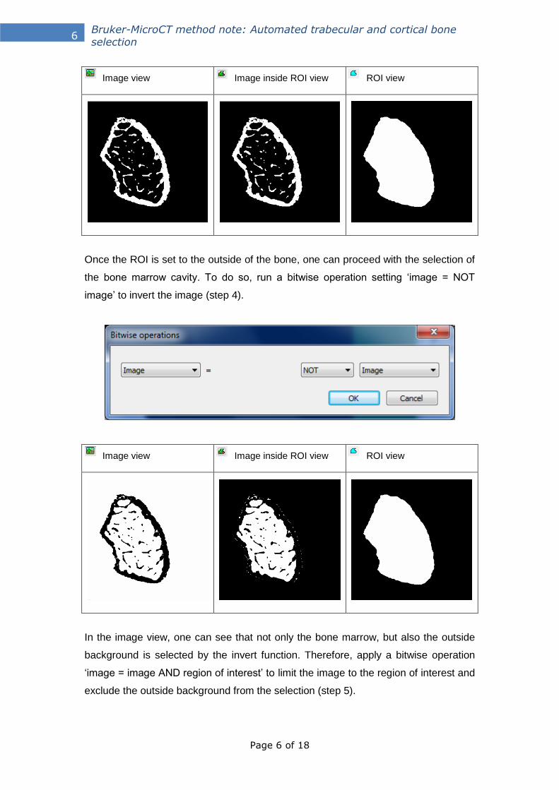
Image view Image inside ROI view ROI view
Once the ROI is set to the outside of the bone, one can proceed with the selection of
the bone marrow cavity. To do so, run a bitwise operation setting ‘image = NOT
image’ to invert the image (step 4).
Image view Image inside ROI view ROI view
In the image view, one can see that not only the bone marrow, but also the outside
background is selected by the invert function. Therefore, apply a bitwise operation
‘image = image AND region of interest’ to limit the image to the region of interest and
exclude the outside background from the selection (step 5).

Page 7 of 18
7 Bruker-MicroCT method note: Automated trabecular and cortical bone selection
Image view Image inside ROI view ROI view
Due to the ROI shrink wrap stretch over holes function, several white speckles
appear at the periosteal surface of the bone which have to be excluded from the
selection. Several despeckling functions can be applied to do so, although a small
opening procedure is more effective in this specific case (step 6).

Page 8 of 18
8 Bruker-MicroCT method note: Automated trabecular and cortical bone selection
Image view Image inside ROI view ROI view
Optionally, remaining white speckles, if any are still present, can be removed by
applying a sweep function in 3D, removing all except the largest object (step7).
Image view Image inside ROI view ROI view

Page 9 of 18
9 Bruker-MicroCT method note: Automated trabecular and cortical bone selection
At this point, the bone marrow is selected but the trabecular bone is not included in
this selection and appears as black speckles or gaps inside the bone marrow
selection. These gaps can be removed by applying a closing function in 2D with a
large radius (step 8). Setting the radius too small will not include trabecula in the
selection that have a thickness larger that the closing radius.
Image view Image inside ROI view ROI view
Following the closing procedure, the bone marrow cavity including the trabecular
bone is selected. However, at slides showing a pore running through the cortical
bone, the selection might include these pore spaces. To limit the bone marrow cavity
selection to the endosteal surface, an opening function can be applied in 2D with a
rather large radius which will result in removal of these spikes and smoothing of the
bone marrow cavity selection (step 9).

Page 10 of 18
10 Bruker-MicroCT method note: Automated trabecular and cortical bone selection
Image view Image inside ROI view ROI view
To make sure the bone marrow cavity selection doesn’t include any parts of thye
cortical bone, a small erosion function is applied, resulting in a bone marrow cavity
selection starting only a few pixels away from the endocortical surface (step 10).

Page 11 of 18
11 Bruker-MicroCT method note: Automated trabecular and cortical bone selection
Image view Image inside ROI view ROI view
In order to be able to save this bone marrow cavity selection as a region of interest
delineating the trabecular bone, as well as a new dataset from this selection, one has
to copy the bone marrow cavity selection to the region of interest by running a bitwise
operation ‘region of interest = COPY image’ (step 11).
Image view Image inside ROI view ROI view
The second last step of the trabecular selection tasklist involves reloading the image
in orde to be able to save a new dataset from the region of the ROI (step 12).

Page 12 of 18
12 Bruker-MicroCT method note: Automated trabecular and cortical bone selection
Image view Image inside ROI view ROI view
The last step is to save a new dataset containing the bone marrow cavity selection
only, as well as the bone marrow cavity selection dataset as a region of interest.
Therefore, save the image inside the region of interest, as well as the region of
interest dataset as a binary selection (step 13).

Page 13 of 18
13 Bruker-MicroCT method note: Automated trabecular and cortical bone selection
Two new folders will be created by default in the ‘VOI trab’ dataset folder, the first
one being the first dataset saved, the second one being the second dataset saved.
The binary ROI dataset can be loaded as a region of interest in the regions of interest
tab in CTan, selecting bitmap files to be loaded instead of a .roi file, either on the
‘VOI trab’ dataset or the newly saved bone marrow cavity selection dataset.
Original 'VOI trab' dataset
with ROI applied
New trabecular selection dataset
with ROI applied

Page 14 of 18
14 Bruker-MicroCT method note: Automated trabecular and cortical bone selection
B. Cortical selection
For the cortical selection, open the ‘VOI cort’ dataset and browse to the custom
processing page. First part of the cortical selection tasklist is basically a
recapitulation of the trabecular selection tasklist. Repeat steps 1 to 10 from the
trabecular selection tasklist (A), to end up with a region of interest corresponding to
the bone cross-sectional area and an image view being the bone marrow cavity
selection.
Image view Image inside ROI view ROI view
Selection of the cortical area now involves dilating the region of interest with a few
pixels to be sure all of the cortical bone is included in the region of interest, followed
by substraction of the bone marrow cavity selection to exclude the trabecular
selection from the cortical region of interest.
First, the region of interest is dilated with a few pixels in 2D to ensure all cortical bone
being included in the region of interest.
Page 15 of 18
15 Bruker-MicroCT method note: Automated trabecular and cortical bone selection
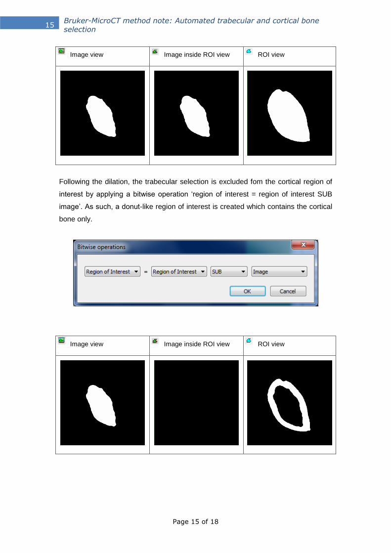
Image view Image inside ROI view ROI view
Following the dilation, the trabecular selection is excluded fom the cortical region of
interest by applying a bitwise operation ‘region of interest = region of interest SUB
image’. As such, a donut-like region of interest is created which contains the cortical
bone only.
Image view Image inside ROI view ROI view

Page 16 of 18
16 Bruker-MicroCT method note: Automated trabecular and cortical bone selection
In analogy with the trabecular seletion tasklist, the image is now reloaded to allow
saving the region of interest as a binary selection, as well as a new dataset of this
region of interest for further analysis.
Image view Image inside ROI view ROI view
Again, the final step is to save a new dataset containing the cortical selection only, as
well as the cortical selection dataset as a region of interest. Therefore, save the
image inside the region of interest, as well as the region of interest dataset as a
binary selection.

Page 17 of 18
17 Bruker-MicroCT method note: Automated trabecular and cortical bone selection
This binary ROI dataset can be loaded as a region of interest in the regions of
interest tab in CTan, selecting bitmap files to be loaded instead of a .roi file, either on
the ‘VOI cort dataset or the newly saved cortical selection dataset.
Original 'VOI cort' dataset
with ROI applied
New cortical selection dataset
with ROI applied

Page 18 of 18
18 Bruker-MicroCT method note: Automated trabecular and cortical bone selection
Part 3: Run the tasklist on multiple datasets using Batch Manager
For high throughput analysis, one can make trabecular and cortical regions
of interest automatically by running the corresponding tasklist to a batch of
bones. To do so, select the ‘Batch manager’ icon in the custom processing tab. The
different steps of the protocol (thresholding, despeckle, bitwise operations, ….) can
be saved in a task list. Therefore each plug-in needs to be added to the task list by
clicking the ‘+’ button (custom processing tab) or ‘add’ button (top level Batch
manager). You can apply the task list to several datasets using batch manager, by
adding the datasets into the bottom part of the batch manager window. Both the task
list and the sample list can be exported if wanted.