Nova Hedwigia . 53 1-2 27-71 Stuttgart, August 1991

Bryophyte response surfaces along climatic, chemical, and physical gradients in peatlands of western Canada

by

L. Dennis Gignac1, Dale H. Vitt2, Stephen C. ZoltaP and Suzanne E. Bayley2

With 10 figures and 6 tables

Gignac, L.D., D.H. Viti, S .C . Zollai & S.E. Bayley (1991): Bryophyte response surfaces along climatic, chemical, and physical gradients in peatlands of western Canada. - Nova Hedwigia 53: 27-71 .

Abstract: The bryophyte component o f peatland vegetation i s analysed for 395 stands o n 335 study sites in western Canada. Sites are located along a broad transect from the Queen Charlotte Islands, British Columbia to southeastern Manitoba. The climate in the study area is divided into five zones: hyper­oceanic, oceanic, suboceanic, subcontinental. A TWINSPAN anl\lysis separated the stands into six groups and selected indicator species for each group. A DCCA ordination showed that surface water che­mistry, climate, and height above the water surface are the most influential gradients distinguishing be­tween stand groups and indicator species. Response surfaces are generated for 31 indicator species along three gradients: pH, height above the water table, and climate as determined by calculating an aridity index. Hyperoceanic , oceanic, and suboceanic fens and bogs are characterized by Sphagnum tenellum. S. austi­nii, S. rubellum, S. papil/osum, Rhytidiadelphus loreus, and Racomitrium lanuginosum. Continental fens and bogs are, in general. characterized by Aulacomnium palustre. These continental mires are further classified into neutral and acidic fens (and bogs) characterized by Sphagnum warnstorjii and wet, extreme-rich fens having Calliergon trijarium, Scorpidium scorpioides. Drepanocladus revol­vens and Campylium stellatum as indicator species . Sphagnum-dominated fens and bogs are dominated by S. magellanicum. S. angustijolium and S. /uscum. Further divisions of the stand classification recog­nized wet poor fens with Sphagnum riparium and S. jensenii; dry fens and bogs with Polytrichum stric­tum, Dicranum undulatum, and Drepanocladus uncinatus; dry poor fens and bogs with Pleurozium schreberi; dry rich/ens with Tomenthypnum nitens, and moderate-rich fens with such indicators as Dre­panocladus aduncus, D. polycarpus. and D. vernicosus. Response surfaces quantify the abundances of individual species along several gradients and are an effi­cient means of determining responses of bryophyte species to various chemical and physical gradients over a broad cimatic regime.

Introduction

Bryophytes are important components of peatland vegetation and in some mire types may dominate all other vegetation. In such oligotrophic acid mires as bogs and poor fens, bryophytes and, in particular, Sphagnum species almost completely cover the peat surface (Sjors 1963, Moore & Bellamy 1974, Horton et al. 1979, Gauthier 1980, Crum 1988). Because of their water holding capabilities and production of H + ions, species of Sphagnum are vital in maintaining high water levels and low pHs that are characteristic of these ecosystems (Clymo 1964, 1967, Hemond 1980, Clymo & Hayward 1982, Hayward & Clymo 1983, Rydin 1985, Rydin & McDonald 1985). In more mesotrophic and alkaline peatlands (rich fens), sedges and other grassy species, as well as bryophytes, characterize the vegetation (Slack et al. 1 980, Karlin & Bliss 1984, Chee & Vitt 1990). Bryophytes may be as abundant in these mires as they are in poor fens and bogs, and play a critical role in nutrient cycling in the ecosystems (Vitt 1 990). Sphagnum species are much less conspicuous in these peatlands, and may be completely absent in those having circumneutral and higher pHs (Slack et at. 1980, Chee & Viu 1990). Other bryophytes, principally brown mos­ses, that are more tolt'iant of high alkalinity and calcium concentrations, are com­mon in these rich fer.>.

The presence, absenCe, and abundance of many bryophyte species have been exten­sively used to define peatland plant communities or associations (Du Rietz 1949, 1954, Sjors 1948, Dansereau & Segadas-Vianna 1952, Ruuhijllrvi 1960, Eurola 1 962, Gauthier 1980, Vitt et al. 1975, Slack et al. 1 980, Chee & Vitt 1990). The plant com­munities have also been characterized by surface water chemistry variables and depth to the water table (Sjors 1952, 1963, Gorham 1956, Gorham & Pearsall 1956). Characteristic or indicator species of these communities are also defined by these variables and thus become not only indicators of the communities but also of ecolo­gical variables (Jeglum 1 971 , Pakarinen 1979, Vitt & Slack 1984). Niche and habitat analyses of Sphagnum species have shown that many of these species have remark­ably high fidelities to such surface water chemistry parameters as pH, conductivity, and Ca + + and Mg + + concentrations, as well as depth to the water table (Vitt et at. 1975, Vitt & Slack 1 975, Horton et al. 1979, Gauthier 1980, Andrus et al. 1983, Vitt & Slack 1984, Gignac & Vitt 1990, Viu et al. 1990). However, the indicator value of a characteristic species is: I) only useful within its geographic range (Chee & Vitt 1990); and 2) may change with regional variation in ecological variables and community structure (pakarinen 1 979). Thus, large scale geographical studies may provide more useful indicators of the vegetation and environmental gradients than regional analyses.

Within the past 20 years, several studies have described plant communities found on a wide variety of peatlands in western Canada (Jeglum 1971, 1972, 1973, Vitt et al. 1975, Zoltai et al. 1 975, Horton et al. 1979, Slack et al. 1980, Zoltai & Pollett 1983, Banner et al. 1986, Banner et al. 1988, Zoltai 1988, Zoltai et al. 1 988, Roche­fort & Vitt 1988, Kubiw et al. 1989, Chee & Vitt 1990, Gignac & Vitt 1990, Nichol­son & Vitt 199Oa, b). Some of these studies have also described the distribution and abundance of the more important bryophyte species within the communities (Hor-

28

ton et al. 1979, Slack et al. 1980, Chee & Vitt 1 990). However, most of these studies were limited to relatively small areas and focussed on the effects of local environ­mental variables on peatland vegetation. These local gradients include: surface water chemistry, height relative to the water table, and shade. Since there is little climatic variation within these relatively small geographic areas, effects of climate on community structure and on individual species distributions were not included. Most studies covering broad geographic areas in western Canada have focussed on producing an inventory of the various types of peatlands found in those areas and describing plants characteristic of them (Zoltai et al. 1975, Zoltai & Pollett 1 983, Banner et al. 1986, Banner et al. 1 988, Zoltai et al. 1988). Although a climatic gra­dient was implicit in these regional studies, their main orientation was towards mire classification or the analysis of the effects of such local environmental variables as surface water chemistry and height above the water surface on the vegetation.

Several studies have shown that peatland development and the distribution of dif­ferent mire complexes are a function of the climate (SjOrs 1 948, Eurola 1962, Moore & Bellamy 1974, Damman 1 977, 1 979). Furthermore, most taxonomic studies o f peatland bryophytes indicate that climate plays a n important role in limiting the geographic distribution of each species (Vitt & Andrus 1 977, Andrus 1980, Janssens 1 983). Thus local or small scale regional gradients that limit species abundances and distribution may be overshadowed by climate. Gignac & Vitt (1990) demonstrated that climate and surface water chemistry were the most important gradients limiting the abundance and distribution of Sphagnum species in western Canada. They also showed that climate and surface water chemistry were highly negatively correlated and that pH, conductivity, and Ca + + concentrations in the surface water generally increased as rainfall and length of the growing season decreased from coastal to con­tinental peatlands in western Canada. Since effects of climate cannot be clearly sep­arated from those of surface water chemistry, any study of climatic effects on peat­land vegetation and species distributions in western Canada must also include sur­face water chemistry variables.

Previous studies of bryophyte species niches or ecotopes (sensu Whittaker et al. 1 983) along several ecological gradients have graphically presented abundance data either as a series of histograms (Watson 1981, Slack 1977, 1982, 1982, Vitt & Slack 1 984) or as smoothed curves (V itt et al. 1975, Slack et al. 1 980, Slack & Glime 1985), where each gradient is treated separately. Although these methods effectively repre­sent the data, they do not show interrelationships either between gradients or be­tween species. Two-dimensional niche analyses have in general produced rectangles or ellipsoids, each representing a different species on one graphic, thus providing valuable ecological information on relationships between species (Watson 1 98 1 , Shaw 1 982, Slack 1982, Dierssen 1 983, Vitt & Slack 1 984, Daniels & Eddy 1985, Gig­nac 1 987). However, rectangles and ellipsoids do not accurately portray species niches along each gradient, since they assume that: 1) species abundances are sym­metrical about a mean, and 2) there are no interactions between gradients. Both as­sumptions are either wrong, or never adequately tested (Watson 198 1 , Jongman et al. 1987).

29

An alternative method of presenting species niche dimensions is to plot species re­sponse surfaces along several gradients simultaneously (Gignac et aI. 1991). This method takes into account the combined effects of two or more gradients on species abundances and for this reason is more accurate than using rectangles to delimit spe­cies niches. Although this method cannot be universally applied since it requires a relatively large data b2.se, it is useful for the more abundant indicator species. In this study, three-dimel·sional response surfaces along three important gradients are generated for importaut species and are used to delimit species ecotopes along those gradients.

The objectives of this study are to: I) distinguish between different communities found in peatlands of western Canada by grouping similar communities based on bryophyte species abundances; 2) select characteristic (indicator) species for each community group; 3) quantify indicator species ecotopes along climatic, physical, and chemical gradients simultaneously using response surfaces.

Study area

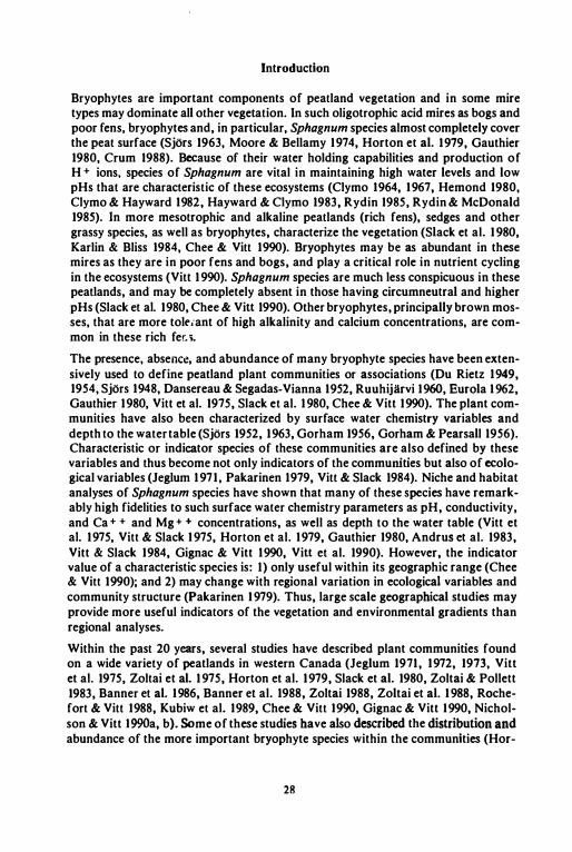
The study area in western Canada includes the central and northern portions of Brit­ish Columbia (including the Queen Charlotte Islands), Alberta, Saskatchewan, and Manitoba, as well as the lowest easternmost corner of Manitoba (Fig. 1 ). This vast geographical area encompasses a wide variety of landforms that include three major mountain ranges and several more topographically homogeneous areas. The study area is bounded to the west by the Coast Mountains, including the Queen Charlotte M ountains, that have elevations between 1 ,500 and 3,000 m, and parallel the coast line (Banner et aL 1988), and to the east and northeast by the Canadian Shield, a peneplain composed of rounded hills having a local relief of less than 1 00 m (Zoltai et al. 1988). The Canadian Shield forms an arc from the northeastern corner of Al­berta the southeastern corner of Manitoba. The two remaining mountain ranges are found in British Columbia and also parallel the coast line. The Hazelton Mountains are adjacent to the Coast Mountains while the Rocky Mountains are on the eastern side of British Columbia. Elevations reach 2,700 m in the Hazelton Mountains and 3,900 m in the Rocky Mountains (Holland 1964). Topographically flatter areas are found between these landforms and include: the Hecate Depression, the Nechako Plateau and Plain, and the Interior Plains (Gignac & Vitt 1990).

The Queen Charlotte Mountains are separated from the Coast Mountains by the ocean-filled Hecate Depression. The terrestrial lowlands of the Hecate Depression include the Queen Charlotte Lowland and several geographically isolated areas on the fringe of the mainland and some of the offshore islands. Elevations in these low­lands are generally below 150 m (Banner et aL 1988). The Netchako Plateau and Plain are found between the Hazelton Mountains and the Rocky Mountains and lie between 1 ,230 and 1 ,500 m above sea level (Holland 1964). The Interior Plains stretch eastward from the Rocky Mountains Foothills to the Canadian Shield and are divided into three parts based on the elevation of the underlying bedrock: 1) the Alberta High Plain (elevation 610-1 ,600 m); 2) the Saskatchewan Plain (elevation 3 20-610 m); 3) the Manitoba Lowland (elevation 220-335 m) (Adams 1988).

10

Figure 1 . Location of the 393 stands studied in western Canada. Ecoclimatic regions are: Gp = prairie grassland; GCD = cordilleran grassland; CB = boreal coniferous; CCD = cordilleran coniferous; CCO = coastal coniferous; SL = low subarctic.

The geomorphology of these landforms is also quite varied. The portions of the Queen Charlotte, Coast, and Hazelton Mountains that are within the study area, and the Canadian Shield are mostly granitic. Granitic bedrock and the soil parent material that is derived from it produce soils that are low in nutrients and CaC03 levels. However, pockets of glacio-lacustrine deposits derived from other sources may occasionally occur in those areas and these deposits can contain higher nutrient levels and CaC031eveis (Zo!tai 1965). The Rocky Mountains, Nechako Plateau and Plain, and Interior Plains are underlain by sedimentary sandstone, limestone, shale, dolomite, and/or coal that are covered by glacial, lacustrine, of fluvial materials (Allan 1943, Green 1 972). Surficial materials generally contain high levels of nu­trients and CaC03 contents are normally very high (Smith et a!. 1 975). However, in some areas CaC031eveis may vary depending on the bedrock from which the soils were formed.

The climate ranges from maritime temperate humid with relatively cool summer temperatures and no long periods of drought along the windward side of the Coast Mountains, to subarctic in isolated pockets in northern Alberta, in northeastern Sas­katchewan, and in northern Manitoba (Zoltai et a!. 1988). A continental, subarctic climate is characteristic by cold winters and short cool summers with extended periods having little precipitation during the growing season. Climatic changes oc­cur abruptly on the western edge of British Columbia because of the effects of the Coast and Hazelton Mountains on the Pacific air masses as they move eastward.

31

East of the Hazelton Mountains, temperature and precipitation gradients are rela­tively small and the climate can be characterised as either subcontinental or conti­nental with cold winters and warm summers (Ecoregions Working Group 1 989). Within the subcontinental region, there is a north-south temperature gradient and an east-west precipitation gradient where the west has lower precipitation than the east.

Materials and methods

Study sites Three-hundred and ninety-three stands were studied on 335 peatlands between 1975 and 1989 (Table I). In this study. peatlands are defined as wetlands having a minimum accumulation of 40 em of peat and a water table that is at or near the peat surface for most of the growing season. Study sites having two or more distinctly different vegetation patterns were divided into stands. All types of peatlands were stu­died including: bogs. poor and rich fens. swamps and some marshes. At least one releve or several quad­rats were taken for each different stand that was present at each site. Based on the Canadian Regional Wetland Classification system (Zoltai 1988 ), study sites are located in the following wetland regions: I ) British Columbia: Oceanic, Oceanic Mountain, and Mid-Boreal; 2 ) Alberta: High. and Mid-Boreal, and Subarctic; 3) Saskatchewan: High- and Mid-Boreal; 4) Manitoba: High-. Mid-. and Low-Boreal.

Table 1. Generalized location. number of �ds studied by each source, sampling year. and vegetation sampling method for 93 stands in western Canada. LocaIion Number

CenIra1 Alberta 1 Northern Alberta 2 CenIra1 Alberta 7 Yukoo 1 CenIraI Alberta 55 CenIra1 Manitoba !1J CoasIaI British Columbia 6 Southern Manitoba 65 CenIra1 Alberta 14 CenIra1 Saskatchewan "Ki CenIra1 Alberta 2 Nor1hem Alberta 1 CoasIaI British Columbia 10 CenIraI British Columbia 0 CenIra1 Alberta 4 CenIra1 Alberta 1 Nor1hem Alberta 1 CenIraI Alberta 63 Nor1hem Alberta 9

Meteorological variables

Source Vitteta!. 1975 Horton et a!. 1979 Slaclt et a!. 1980 Horton(un� ZoItai &: J �unpubR ZoItai .t. Johnson unjlubl Vittetal.l990 Zoltai .t. Johnson (unpubl) Chee.t. Vittl990 Zoltai .t. Jolmson (unpubl) Kubiw et a!. 1989 Nicholson .t. Vilt 1990b Gignac .t. Vilt 1990 Gignac .t. Vilt 1990 Gignac .t. Vilt 1990 RoChefort .t. Vilt 1988 Nicholso n ��bl) Nicholson itt 19908 Zoltai .t. Johnson (unpubl)

Yea- MeIhod 1974 quadrat 1976 quadrat 1976 quadrat 1918 meve 1981 ldev6 1982 JeIcve 1983 JeIcve 1983 JeIcve 1984 quadrat 1984 meve 1984-85 JeIcve 1984-85 JeIcve 1985-87 quadrat 1986 quadrat 1986 quadrat 1986 quadrat 1988 JeIcve 1988-89 JeIcve 1989 JeIcve

MeteorOlogical data w�s obtained from 3O-year means (1951- 1980) measured at the nearest permanent weather station to each site (Anonymous 19818, b, 1986) (Table 11). The following variables were calcu· lated for each station: I) Length of growing season (OS), calculated as the number of days having mean temperatures above ZOC; 2) Precipitation (P). calculated as the total amount of rainfall during the grow­ing season; 3) biotemperature (Bt), which is the summation of mean monthly temperatures above 2°C divided by 12 (Tuhkanen 1980, 1984). A temperature threshold of 2°C was used to calculate each vari· able. since there is no measureable amount growth for mosses below that temperature (OUme 1982). An aridity index (AI) was calculated as:

P AI= ---

T+lO

where T is the mean annual temperature.

Vegetation sampling Bryophyte abundance was estimated as percentage cover by the canopy method (Daubenmire 1959. Vilt et al. 1915) for each stand present on a site. Quadrat sizes and sampling designs are as follows: 25 X 25 cm restricted random (Vilt et al. 1915. Horton et al. 1919. Slack et a1. 1980. Chee & Vilt 1990); 50x 100 cm systematic (Gignac & Vilt 1990); I x I m systematic (Rochefort & Vilt 1988). Releve sizes and samp­ling techniques also varied: 3 (6 x 6 m) random (Nicholson & Vilt 199Ob); SO m diameter circular random (Nicholson & Vilt 19903. Kubiw et al. 1989); systematic by stand (Zoltai & Johnson unpublished). Of the 110 bryophyte species found in this study. the ninety most abundant are reported here. Nomenclature follows Ireland et a1. 1981. with the exception of Sphagnum austinii (Andrus 1987) and Sphagnum pacifi­cum (Flatberg 1989).

Environmental variables Water samples were collected for each stand. either from surface water in natural depressions or. where no surface water was available. from the water that accumulated in shallow pits dug in the peat. pH measurements were taken either in situ by inserting the probe directly into the surface water. or from water samples shortly after they were collected. Conductivity was also measured shortly after sampling. and calculated as corrected conductivity (kcorr) by correcting to 20·C and for H + ions (Sjllrs 1952). Elemental concentrations (Ca. Mg. Na. K) were measured in each water sample either on an atomic ab­sortion spectrophotometer or on an inductively coupled argon plasma spectrophotometer. For the purpo­ses of this study. elemental concentration units are reported as mg I-I.

The height of moss plants above the water surface was also determined for each stand. Height measure­ments were either taken directly be measuring the distance from the surface water to the top of the moss plants or peat surface (Gignac and Vilt 1990. Zoltai & Johnson unpUblished) or indirectly by assigning a microtopographc category to a Quadrat or releve (Chee & Vilt 1990). Microtopographic categories were based on decimetre classes from -I to 9 where -I = 0 to 10 cm below the surface of the water and 9 = 90 to 100 cm above the surface water. Height measurements that were taken directly were rounded to the nearest decimeter.

Water levels vary from year to year and may fluctuate up to 1.5 dm between spring runoff and summer drought conditions (0kland 1989). Measurement of height above the water surface are also affected by the amount of rain that has fallen prior to sampling and the length of time between sampling and rain events. Since water level fluctuations are specific to each peatland. accurate water level measurements require sampling each study site several times over the course of several years. However. because of the distances involved and the large numbers of sites. height above the water surface measurements were tak­en only once. usually during the summer. and seasonal variations were not recorded. Undoubtedly. height measurements would have been much more accurate if they were corrected to the same distance below the high water mark on each site. However. because of the lack of seasonal data. no altempt was made to correct for yearly water level fluctuations. fluctuations during the summer. or yearly differences. As a result. species response surfaces may be wider along the height gradient than if the measurements had been corrected to the same level on each site.

Data analyses Species abundances were subjected to a TWINSPAN analysis. a divisive hierarchial method the produces a two-way clasification of species and stands (Hill 1919). This analysis also identifies species that are diagnostic of each stand division in the classification (indicator species). Species abundances and environ­mental and climatic variables were ordinated simultaneously using a detrended canonical correspondence analysis (DCCA) (ter Braak 1981). All 110 species were used in both analyses.

Three-dimensional response surfaces are generated for indicator species along climatic, surface water chemistry, and depth to the water table gradients. Response surfaces are produced by gridding observed

33

abundance data using distance-weighted means (Gignac et at. 1991). This method also sets outlier abun­dance values using distance-weighted means. Other results of the smoothing process are to: I) interpolate abundance values within species ranges, thus filling sampling gaps; 2) extrapolate species ranges by one grid node along all three gradients.

All computations and statistical analyses were done on a microcomputer using the Statistical Analysis System (SAS) package. Three-dimensional response surfaces were graphed using Proc G3D from SAS graph.

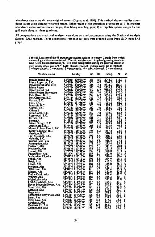
Table II. Location of !he 98 �t weather stations in western canada from which meteorological data was obtilined_ Climatic variables are: length of growing season in days (GS); biotemperature in "C (Bt); IOtaI JRCipitation during !he growing season in mm' aridity index in mm "C" I (AI); c:1imafc lDIIC (Z). Climate zones are as follows: I = hyperoceanic; 2 = oceanic; 3 = suboceanic; 4 = subcontinental; 5 = continental.

Weather station Locality GS Bt Ptec:ip />J Z

Bonilla Island, B.C. 53"30'N \30038'W 36S 8.0 2041.0 113.3 I Prince Rupert A, B.C. S4°18'N 130"26'W 302 6.7 2369.0 151.1 I Prince Rupert Mont Cin: S4°19'N 130"26'W 346 7.4 2334.9 180.1 I Prince Rupert S4°17'N 130023'W 347 7.4 2334.9 138.1 1 Prince Rupert � S4°1S'N l3O"2O'W 302 6.7 2185.3 178.6 1 Prince Rupert hawadans S4OZ0'N 13O"15'W 346 7.4 2957.9 170.0 I Falls River, B.C. 53°59'N 129°44'W 297 6.7 3358.7 178.7 1 Pon Clements, B.C. 53°41'N 132°llW 315 7.5 1328.2 82.1 2 Masset, B.C. S4002'N 132°08'W 326 7.1 1237.8 78.0 2 Tlell,B.C. 53OZ9'N 131°S6'W 335 7.4 1091.2 62.7 2 Sandspit. B.C. 53°15'N 131°49W 36S 7.9 1199.7 67.0 2 Kitimat, B.C. S4003'N 128°42'W 242 7.0 1282.0 78.2 3 Kitimat2 S4000'N 128°42'W 251 7.3 1253.0 77.1 3 Bella Coola, B.C. 52OZ2'N 126°41 'W 267 7.8 1092.0 81.4 3 Rosswood. B.C. 54°51'N 128°4S'W Z26 6.6 so 1.3 52.6 4 Terrace, B.C. S4 "JO'N 128°37'W 241 7.1 564.7 58.0 4 TenaceA. S4"28'N 128°35'W 231 6.8 605.1 58.8 4 Prince George, B.C. 53°53'N 122°4O'W 20S 5.5 473.9 40.4 4 Dome Creek. B.C. 53°44'N IZOO59'W 20S 5.5 473.9 40.5 4 Mount Robson Ranch, B.C. 53001'N 119°14'W 196 5.2 285.8 41.0 4 Tapley Landing, B.C. S4°59'N 126°10'W 194 5.2 267.8 22.9 5 HaZelton, B.C. SS012'N 127°44'W 220 6.1 320.8 27.4 5 Fort St-James, B.C. S4OZ7'N 124° 15'W 197 5.5 266.1 23.6 5 Mcbride. B.C. 53°16'N 120009'W 212 6.3 330.9 28.6 5 Watson Lake, Yuk. 60007'N 128°49'W 165 4.6 216.2 27.1 5 Assumption, Alia 58°42'N 118°41 'W 178 5.3 275.4 35.8 5 �Alla 53OZ2'N 117°42'W 195 5.3 341.2 28.S 5 NotikewlO, Alia 57001'N 117°34W 182 5.5 251.5 28.5 5 Hinton, Alia 53OZ5'N 117°34 'W 196 5.4 388.0 31.3 5 Peace River, Alia S6°14'N 117°26'W 189 5.7 252.0 25.1 5 Valleyview RS, Alia 55004'N 1I7°16W 200 6.1 326.6 29.6 5 Fabler, Alia 55°44'N 117°12'W 190 5.8 294.9 28.1 5 Robb,Al1a 53°14'N I J6058'W 188 4.9 413.3 36.2 5 Ed.wn,AlIa 53"35'N 1160Z7'W 188 5.1 386.0 36.1 5 Nordegg, Alia 52OZ9'N 116005'W ISS 4.3 382.1 35.8 5 WhiteCOwt. Alia S400s'N 11S"4O'W 191 5.5 385.4 35.3 5 Kinuso, Alia 55OZ0'N 115°26'W 194 5.8 357.0 33.6 5 Prairie CreeIc, Alia 5Z015'N 11S"18'W In 4.3 422.4 42.2 5 Wap:r, Alia 55OZI'N 114°59'W 188 5.5 306.2 30.1 5 Moon Lake. Alia 53OZ8'N 1l4"59'W 194 5.7 380.0 32.8 5 Fan Assiniboine, Alia S4OZ2'N 1l4"55'W 187 5.6 356.3 33.1 5 Rock}' Mountain House, Alia 52OZ3'N 114°55'W 197 5.8 385.8 30.9 5 Slave Lake. Alia 55°17'N 114°46'W 191 5.7 340.2 32.2 5 Glenevis, Alia 53°48'N 114°3 rw 196 5.8 379.9 32.7 5 Vega, Alia 54OZ4'N 1l4"23'W 194 6.0 389.4 33.7 5 Edmonton Stoney Plain, Alia 53°33'N 114006W 198 6.2 380.3 32.3 5 Smi1h,A11a 55°10'N lWOZ'W 187 5.6 359.2 35.6 5 Cross Lake, Alia 54°38'N 113°S4'W 188 5.4 377.7 38.5 5 A�1a S4°49'N I W32W 195 6.1 346.4 30.9 5 Meanook S, Alia S4"37'N 1130zrW 196 6.2 354.0 30.0 5 Calling Lake. Alia 55°15'N 113°11'W 193 5.6 353.2 34.6 5

34

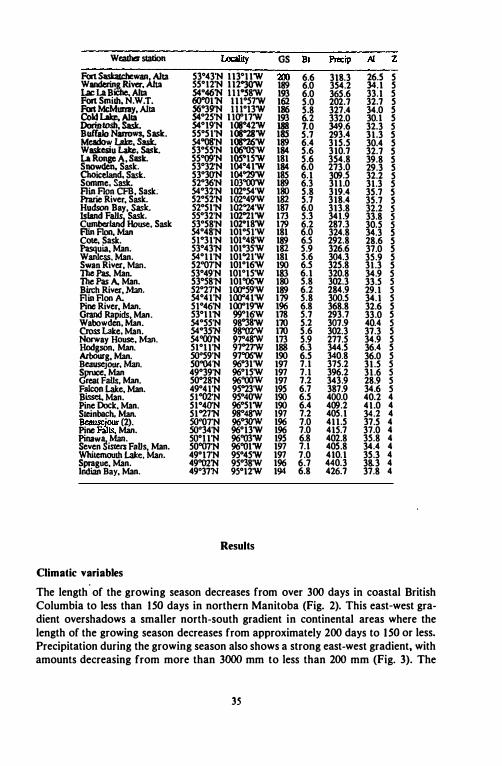
Wtalber station Locality GS Bt Precip />l Z Fort Sasblcbcwan Alta 53°43'N 113°11'W :m 6.6 318.3 26.5 5 Wandering River, Ahi S5°12'N 112"3O'W 189 6.0 354.2 34.1 5 Lac La BiChe. Alta S4°46'N lllOS8'W 193 6.0 365.6 33.1 5 Fort Smilil, N.W.T. 6()OO1'N 111°S7'W 162 5.0 202.1 32.1 5 Fort MtMunay,Alta S6"l9'N lllol3'W 186 5.8 327.4 34.0 5 Cold LaIce, Alta S4"2S'N 1l0"11'W 193 6.2 332.0 30.1 5 DorinIOSh. Sask. S4°19'N 108"42'W 188 1.0 349.6 32.3 S Buffalo Nanows, SasIc. 55°51'N 1(J802g'W ISS 5.1 293.4 31.3 5 Meadow Lab:, Sask. S4008'N 108"26'W 189 6.4 315.5 30.4 5 Wastesiu Lab:, Sask. 53°55'N 10600S'W 1&4 5.6 310.1 32.1 5 La Rooge A. Sask. 55009'N 10s015'W 181 5.6 354.8 39.8 5 SlIOwdCII. Sask. 53"l2'N 104°41'W 1&4 6.0 213.0 29.3 5 Choiceland. SasIc. 53°3O'N 104"29'W ISS 6.1 309.5 32.2 5 Somme, SasIc. 52'36'N 103"OO'W 189 6.3 311.0 31.3 5 Flin FIon CFB. Sask; S4°32'N 102°S4'W lllO 5.8 319.4 35.1 5 Prarie River. Sask. 52°52'N 10'2"49'W 182 5.1 318.4 35.1 5 Hudson Bay. Sask. S2°SI'N 102"24'W 187 6.0 313.8 32.2 S Island Fr!/ Sask. Sso32'N 102"21'W 113 S.3 341.9 33.8 S Cumberlan House. Sask S3°58'N 10'2"18'W 179 6.2 281.3 30.S S FUn Ron. Man S4°48'N 101oSl'W 181 6.0 324.8 34.3 5 COle. Sask. Sl°31'N 10Io48'W 189 6.S 292.8 28.6 5 �uia.Man. S3°43'N 101"lS'W 182 S.9 326.6 37.0 5 Wariless. Man. S4°11'N 101"21'W 181 S.6 304.3 3S.9 5 Swan River. Man. 5200TN 10lo16'W 190 6.S 325.8 31.3 5 The Pas, Man. S3°49'N 10101S'W 183 6.1 320.8 34.9 S The Pas A. Man. 53°S8'N 1010Q6'W lllO S.8 302.3 33.S S Birch River. Man. S2"2TN l00"S9'W 189 6.2 284.9 29.1 S Rill Ron A. S4°41'N l00"41'W 179 S.8 300.S 34.1 S Pine River. Man. Slo46'N l00"19'W 196 6.8 368.8 32.6 5 Grand Rapids. Man. S3°11'N WI6'W 178 S.1 293.7 33.0 5 Wabowden. Man. S4°SS'N 98"3&'W 110 5.2 301.9 40.4 S Cross Lake, Man. S4°3m 98"02'W 110 5.6 302.3 31.3 5 Norway House. Man. S4"OO'N 97"48'W 113 5.9 271.S 34.9 5 Hodgson. Man. SI°11'N 91"21'W 188 6.3 344.5 36.4 5 ArbOurg. Man. s00S9'N 970Q6'W 190 6.5 340.8 36.0 S Beausejour, Man. SOOO4'N 96"lI'W 197 7.1 37S.2 31.S S �.Man 49'39'N 96°1S'W 197 7.1 396.2 31.6 S

real Falls, Man. SO"28'N 96"OO'W 197 1.2 343.9 28.9 S FaIcQn Lake. Man. 49°41'N 9S"23'W 195 6.7 387.9 34.6 S Bisset. Man. SI002'N 9S°4O'W 190 6.5 400.0 40.2 4 Pine Dock, Man. SI°4O'N 96°S1'W 190 6.4 409.2 41.0 4 Steinbach, Man. SI"27'N 98"48'W 197 7.2 405.1 34.2 4 Beausejour (2). SOOOTN 96"3O'W 196 7.0 411.5 37.5 4 Pine Falls. Man. s0034'N 96°13'W 196 7.0 41S.7 37.0 4 PinaW� Man. sool1'N 96003'W 195 6.8 402.8 3S.8 4 Seven isters FaDs. Man. SOOO7'N 96001'W 197 7.1 405.8 34.4 4 Whilel1loulil Lake. Man. 49°1TN 9so4S'W 197 7.0 410.1 35.3 4 Sptague. Man. 49"02'N 9S"l8'W 196 6.7 440.3 38.3 4 Iridian Bay. Man. 49"l7'N 9so12'W 194 6.8 426.1 37.8 4

Results

Climatic variables

The length' of the growing season decreases from over 300 days in coastal British Columbia to less than ISO days in northern Manitoba (Fig. 2). This east-west gra­dient overshadows a smaller north-south gradient in continental areas where the length of the growing season decreases from approximately 200 days to ISO or less. Precipitation during the growing season also shows a strong east-west gradient. with amounts decreasing from more than 3000 mm to less than 200 mm (Fig. 3). The

35

north-south gradient in continental areas is more complex: 1) in eastern British Co­lumbia. Alberta. and Saskatchewan. precipitation is approximately 200 mm in the south. increases to over 300 mm in the central areas and decreases again to approxi­mately 200 in the northern portions of those provinces: 2) in Manitoba precipitation decreases from north to south. Both east-west and north-south gradients are again prevalent for biotemperature. but the south to north gradient is more important than the east-west gradient. The biotemperature decreases south to north from 1 0 to 6°C i n continental areas.

The aridity index is more complex than the other climatic variables. combining both temperature and precipitation factors. Index values decrease from coastal British Columbia to Alberta then increase to eastern Manitoba (Fig. 5). Values also increase from southern Alberta to northeastern Manitoba. An aridity index value of 20 mm °C-I in the southern portion of the study area roughly coincides with the Great Plains semiarid and 10 ..... elevation Cordilleran grasslands (Fig. 1). A value of 30 mm °C-I in the southern areas approximately the transitional grassland and the conifer­ous forest. This line aiso indicates the southern limit of peatiand formation in we­stern Canada (Zoltai 1975). The index value of 50 in northern Manitoba and north­eastern Saskatchewan coincides with the low subarctic ecological region.

Figures 2-5. lsopleths of four climatic variables plotted for western Canada. - 2. Length of growing sea­son (days). - 3. Precipitation during growing season (mm). - 4. Biotemperature (0C). - S. Aridity index (mm OC-I).

Based on length of growing season and precipitation during the growing season, the climate in the study area can be divided into 5 zones (Table II). Hyperoceanic areas have growing seasons of 300 or more days, and over 2,000 mm of precipitation. Oceanic areas also have growing seasons over 300 days, but less precipitation ( 1000 to 1600 mm). Suboceanic areas have growing seasons between 200 and 280 days and over 1 000 mil) of precipitation. The subcontinental zone has more than 190 growing days and between 400 and 700 mm of precipitation. Continental areas have less than 400 mm of. rain during the growing season.

Chemical variables

Water chemistry variables vary widely between sites and climatic zones (Table Ill). With the exception of Na and K concentrations, mean values for all chemical vari­ables are higher in subcontinental and continental areas than for the other climatic zones. Mean Na concentrations are highest in oceanic areas, while K concentrations are highest in suboceanic areas. pH and Ca values ranges from 3.7 to 6.9, and 0.05 to 14.81 mg I-I in hyperoceanic areas. In oceanic areas, pH and Ca values range from 4.1 to 4.5, and 0.25 to 1 .27 mg I-I . In the suboceanic climate zone, pH values are constant at approximately 5 . 1 and Ca concentrations range from 0.66 to 4. 1 1 mg I-I . These narrow pH and Ca ranges are related to the small number of study sites in the suboceanic zone. In subcontinental and continental areas, minimum pH (3.0) and Ca concentrations (0.01 mg H are slightly lower and maximum pH (8.2) and Ca (146.61 mg I-I ) are higher than in any other climate zone. Among the chemical variables analysed in surface water, pH, Kcorr, Ca and Mg val­ues are highly significantly correlated (p>O.OOI) (Table IV). These variables are sig­nificantly negatively correlated (p<O.OS) with such climatic variable as growing sea­son, precipitation, and aridity index. Sodium is not significantly correlated with Ca and Mg (p<O.OS). All climatic variables are highly significantly correlated (p<O.OOI), however correlation coefficients are highest for the relationship between precipitation, growing season, and aridity index.

Table III. Mean ± SIaIIdard deviation for pH. com:cled conductivity , kcorr (IJS). and elemental concenlllllions (mg 1,1) for surface water collected from 393 stands in western Canada. CIimaIe zones are: 1 .. byperoceanic; 2 .. oceanic: 3. suboceanic: 4 = subcontinental; S. conlinental. n .. number of sites within each climate zone.

zme pH talT 01 f>i NIl K n

1 s.2±l.o 25.0£18.9 O.81±1.26 0.46±O.23 2.23±O.86 O.I5±O.29 :& 2 4.2±O.1 82.1±19.1 O.43±O.l7 1.61±O.34 13.96±2.01 O.lS±O.4S 10 3 S.l±O.l SO.0±39.3 2.6l±1.77 O.43±O.19 4.06±Z.23 4.22±2.01 3 4 S.7±l.1 33S.8±23S.4 2S.48±2S.00 9.94±7.08 3.00±1.83 1.4O±O.76 44 S S.7±1.1 2OS.3±218.S 19.83±23 .91 6.S2±7.66 6.1l±22.08 l.SO±2.08 3U1

37

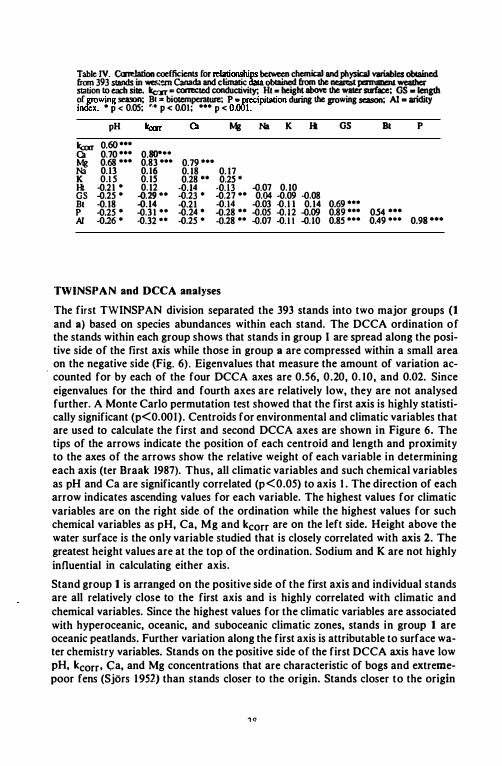
Table IV. CmeIaliOll coefficients for relationships between chemical and physical variables obcained from 393 SI8IIds in ..-.= Canada and climatic daJa obIained from the IIe8Iat � wcaIhcr station 10 each site. Itcarr .. corrected conductivity; Ht .. height above the water surface; OS -lengdl of growing season; BI" biolempemture; p .. precipitation during the growing season; AI .. aridity index. • p < O.OS; , .• P < O.ol; ••• p < 0.001.

� � K HI OS Bt P )J

pH

0.60··· 0.70··· 0.68··· 0.13 O.IS

.o.21 • .o.2S • .o.18 .o.2S • .o.26 •

0.80*·· 0.83··· 0.16 0.15 0.12 '().29 ••

'()J4 .o.31·· .o.32··

Mg Na K Il

0.79··· 0.18 0.17 0.28·· 0.25·

.oJ4 .oJ3 .o.07 0.10

.o.23 · .o.27·· 0.04 .o.09 .o.08

.o.21 .oJ4 .o.03 .oJ I 0.14 .o.24· .().28·· .o.OS .o.t2 .o.09 .o.2S· .().28·· .o.07 .oJ I .o.tO

TWINSPAN and DCCA analyses

OS Bt P

0.69··· 0.89··· 0.54 ••• 0.85 ••• 0.49 ••• 0.98 •••

The first TWINSPAN division separated the 393 stands into two major groups (1 and a) based on species abundances within each stand. The DCCA ordination of the stands within each group shows that stands in group I are spread along the posi­tive side of the first axis while those in group a are compressed within a small area on the negative side (Fig. 6) . Eigenvalues that measure the amount of variation ac-

. counted for by each of the four DCCA axes are 0.56, 0.20, 0. 10, and 0.02. Since eigenvalues for the third and fourth axes are relatively low, they are not analysed further. A Monte Carlo permutation test showed that the first axis is highly statisti­cally significant (p<O.OOI). Centroids for environmental and climatic variables that are used to calculate the first and second DCCA axes are shown in Figure 6. The tips of the arrows indicate the position of each centroid and length and proximity to the axes of the arrows show the relative weight of each variable in determining each axis (ter Braak 1987). Thus, all climatic variables and such chemical variables as pH and Ca are significantly correlated (p<0.05) to axis 1 . The direction of each arrow indicates ascending values for each variable. The highest values for climatic variables are on the right side of the ordination while the highest values for such chemical variables as pH, Ca, Mg and kcorr are on the left side. Height above the water surface is the only variable studied that is closely correlated with axis 2. The greatest height values are at the top of the ordination. Sodium and K are not highly influential in calculating either axis. Stand group 1 is arranged on the positive side of the first axis and individual stands are all relatively close to the first axis and is highly correlated with climatic and chemical variables. Since the highest values for the climatic variables are associated with hyperoceanic, oceanic, and suboceanic climatic zones, stands in group 1 are oceanic peatlands. Further variation along the first axis is attributable to surface wa­ter chemistry variables. Stands on the positive side of the first DCCA axis have low pH, kcorr, ea, and Mg concentrations that are characteristic of bogs and extreme­poor fens (Sjors 1 952) than stands closer to the origin. Stands closer to the origin

1Q

400

200

C\I � 0

-200

-400 -200

r·····················-·-···-··· .. ············� 300 [HII ! ConUnental t.oos & � �rICh fen. poor tent i Ln ........................................... _.; go o

o

-100

o o

o

o

! I I

f ! I : : :

i 00 111

1 1, � 9 f f ! ! f····································oceanic················································1 I bogs. ! lmoderale-rlch fens ... treme-poor fens ! t .................................... ......................................................... .3

100 200 300 400 500 Axis 1

Figure 6. DCCA ordination of the 393 stands analysed in western Canada. Stand group one (I) is separa· ted from remaining continental stands (a) - see Fig. 8. Insert: DCCA ordination of climatic and environ­mental variables. Heads of arrows indicate the coordinates of the centroid for each variable. Parentheses indicate variables that are significantly correlated (p<O.05) with the first axis. Brackets indicate signifi­cant correlations with the second axis. Abbreviations are: Ht = height of moss plants above the water surface; Bt = biotemperature; GS = length of growing season; P = precipitation during growing sea­son; AI = aridity index; kcorr = corrected conductivity; plus standard ionic and elemental abbreviations (pH, Ca, K, Mg, Na).

have high pH, kcorr, Ca, and Mg values that are associated with rich fens (Sjors 1952). Thus, although stands in group 1 are all found in oceanic areas, they also ordinate along a water chemistry gradient.

Group a contains 344 stands that are almost exclusively found along the negative side of the first axis and are thus found in subcontinental and continental areas. Stands within these climatic zones are also ordinated along a surface water chemis­try gradient. Stands closer to the origin have relatively low pH, kcorr, Ca, and Mg values and are bogs and poor fens. Stands having high negative values have high pH, kcorr, Ca, and Mg concentrations and are rich fens.

Because of the large number and the distribution of stands in group a, it is difficult to determine where subsequent TWINSPAN divisions lay on the DCCA ordination, and as a result, it was also difficult to determine effects of the environmental varia­bles on stand groups. Therefore, stands in group a were subjected to further TWIN­SPAN and DCCA analyses in an attempt to clearly demonstrate the eff eets of envi­ronmental and climatic variables on stand groupings and their ordination. The

39

TWINSPAN analysis of continental mires separates the stands into five groups (Fig. 7). 11Ie first separation divides group 6 (eigenvalue = 0.62) from the remaining stands. The next division (eigenvalue = 0.48) separates group 5, while the third divi­sion (eigenvalue = 0.33) separates group 2 from the remaining stands. Groups 3 and 4 are separated by the fourth division (eigenvalue = 0.29) and are the most similar.

Eigenvalues for the four axes resulting from the DCCA analysis of continental stands are 0.49. 0.23. 0. 1 1 , and 0.04. As is the case for the original DCCA analysis, eigel1Ylllues for the third and fourth axes are relatively low and are not analysed further. A Monte Carlo test for the DCCA ordination of continental stands indi­cates that axis I is highly significant (p<O.O I ). Such chemical variables as pH, kcorr •• and Mg are significantly correlated (p<O.OS) with the first axis while height above the water surface (Ht) is significantly correlated with the second axis (Fig. 8). The directions of the two arrows indicate that the lowest pH. kcorr• and Mg values are oa the positive side of the first axis and the highest values are on the negative side. The greatest height above the water surface values are on the positive sides of both lXes I and 2. Sodium, K. and all climatic variables are not significantly corre­lated with either the first or second axis.

STAND GROUPS

-Rich lens

Figure 1. Dendogram showing the six stand groups resulting from two TWINSPAN analyses of 393 stands ill western Canada. The first TWINSPAN analysis produced stand group 1. The second analysis dividedlhe remaining 344 continental stands into stand groups 1 to 6. Values. descriptions. and abbrevia­tions • each division indicate eigenvalues. peat land types. and indicator species. respectively for each cut level. Abbreviations correspond to the first three letters of species names as listed in Table VI.

400

200

C\I

'00

WeI moderale.nch lens __ -::=-*" ____ Axis t 5 5 .... ...

55 5'>§�

(Mol 5 �6 6 Dry tllccm) -200 515 gs 5 5 rich fens Ails 2 6�5 5 5SS� 5 5 3

i 0 6 � tfss5 �� 4 �� 6 ��s%�!�!\4�:���;f 3

.

lif 5 '55 65 1 3 2 � 2 . rYpoorlens & bogs

-200 ��,,'W'6 5 425 22 i'ijl'<> WeI poor lens

6 WeI extreme-rich lens

-400T-------�----�------�------�----� - 300 -200 -100 o 100 200

Axis 1

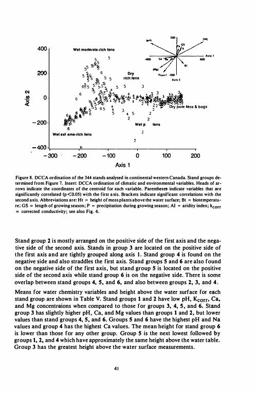
Figure 8. DCCA ordination of the 344 stands analysed in continental western Canada. Stand groups de­termined from Figure 7. Insert: DCCA ordination of climatic and environmental variables. Heads of ar­rows indicate the coordinates of the centroid for each variable. Parentheses indicate variables that are significantly correlated (p<O.05) with the first axis. Brackets indicate significant correlations with the second axis. Abbreviations are: Ht = height of moss plants above the.water surface; Bt = biotemperatu­re; GS = length of growing season; P = precipitation during growing season; AI = aridity index; kcorr = corrected conductivity; see also Fig. 6.

Stand group 2 is mostly arranged on the positive side of the first axis and the nega­tive side of the second axis. Stands in group 3 are located on the positive side of the first axis and are tightly grouped along axis 1_ Stand group 4 is found on the negative side and also straddles the first axis. Stand groups 5 and 6 are also found on the negative side of the first axis. but stand group 5 is located on the positive side of the second axis while stand group 6 is on the negative side. There is some overlap between stand groups 4, 5, and 6, and also between groups 2, 3, and 4 . Means for water chemistry variables and height above the water surface for each stand group are shown in Table V. Stand groups 1 and 2 have low pH, Kcorr• Ca, and Mg concentraions when compared to those for groups 3, 4, 5, and 6. Stand group 3 has slightly higher pH. Ca. and Mg values than groups 1 and 2. but lower values than stand groups 4, 5, and 6. Groups 5 and 6 have the highest pH and Na values and group 4 has the highest Ca values. The mean height for stand group 6 is lower than those for any other group. Group 5 is the next lowest followed by groups 1, 2, and 4 which have approximately the same height above the water table. Group 3 has the greatest height above the water surface measurements.

41

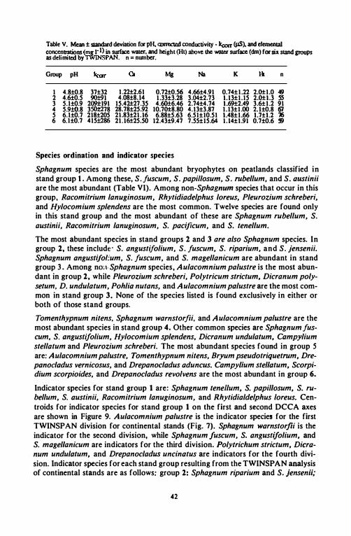
Table V. Mean ± standard deviation foe PH. COIRICIed conductivity - kcorr WS), and e1emenlal concenlJations (mg I-I) in surface water, and height (Ht) above !he water surface (elm) for six stand groups as delimited by lWINSP AN. n = nmober.

Group pH

I 4.8±O.8 37±32 2 4.6±O.S 9O±91 3 S.I±O.9 209±191 4 S.9±O.8 350±278 S 6.I±O.7 218±2OS 6 6.I±O.7 4IS±286

1.22±2.61 4.08±8.14

IS.42±27.3S 28.78±2S.92 2\.83±21.\6 21.16±2S.SO

Mg Na K n

O.72±O.S6 4.66±4.91 O.74±1.22 2.0±1.0 49 1.33±3.28 3.04±2.73 1.13±I.IS 2.0±1.3 55 4.60±6.46 2.74±4.74 1.69±2.49 3.6±1.2 91

IO.70±8.80 4.13±3.87 1.13±I.00 2.1±O.8 61 6.88±S.63 6.SI±IO.SI 1.48±1.66 1.7±1.2 "Xi

12.43±9.47 7.SS±IS.64 1.14±1.91 O.7±O.6 !9

Species ordination and indicato r species

Sphagnum species are the most abundant bryophytes on peatlands classified in stand group 1. Among these, S. juscum, S. papi/losum, S. rubellum, and S. austinii are the most abundant (Table VI). Among non-Sphagnum species that occur in this group. Racomitrium lanuginosum, Rhytidiadelphus loreus, Pleurozium schreberi, and Hylocomium splendens are the most common. Twelve species are found only in this stand group and the most abundant of these are Sphagnum rubellum, S. austin ii, Racomitrium lanuginosum, S. pacijicum, and S. tenellum.

The most abundant species in stand groups 2 and 3 are also Sphagnum species. In group 2, these include' S. angustijolium, S. juscum, S. riparium, and S. jensenii. Sphagnum angustijot:um, S. juscum, and S. magellanicum are abundant in stand group 3 . Among nml· Sphagnum species. Aulacomnium palustre is the most abun­dant in group 2, while Pleurozium schreberi, Polytricum strictum. Dicranum poly­setum, D. undulatum, Pohlia nutans, and Aulacomnium palustre are the most com­mon in stand group 3. None of the species listed is found exclusively in either or both of those stand groups.

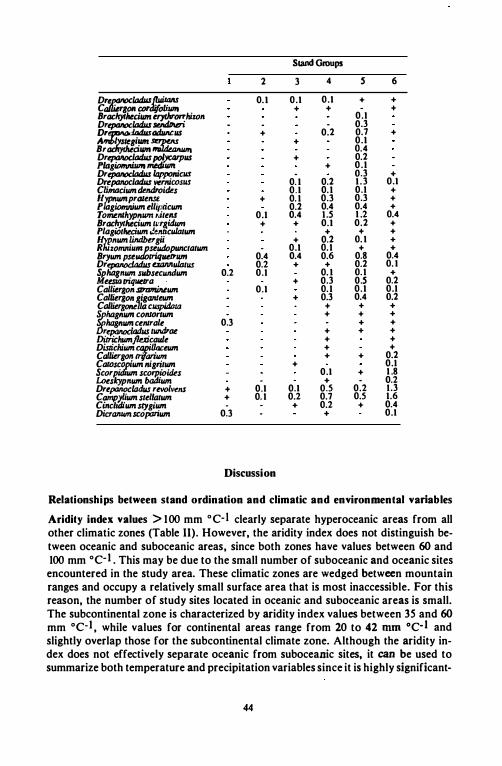
Tomenthypnum nitens, Sphagnum warnstorjii, and Aulacomnium palustre are the most abundant species in stand group 4. Other common species are Sphagnum jus­cum, S. angustijolium, Hylocomium splendens, Dicranum undulatum. Campylium stellatum and Pleurozium schreberi. The most abundant species found in group 5 are: Aulacomnium palustre, Tomenthypnum nitens, Bryum pseudotriquetrum. Dre­panoc/adus vernicosus, and Drepanoc/adus aduncus. Campy/ium stellatum. Scorpi­dium scorpioides, and Drepanoc/adus revolvens are the most abundant in group 6. Indicator species for stand group 1 are: Sphagnum tenellum. S. papillosum. S. ru­bellum, S. austinii, Racomitrium lanuginosum, and Rhytidialdelphus loreus. Cen­troids for indicator species for stand group 1 on the first and second DCCA axes are shown in Figure 9. Aulacomnium palustre is the indicator species for the first TWINSPAN division for continental stands (Fig. 7). Sphagnum warnstorfii is the indicator for the second division, while Sphagnum juscum, S. angustijolium. and S. magellanicum are indicators for the third division. Polytrichum strictum. Diera­num undulatum. and Drepanocladus uncinatus are indicators for the fourth divi­sion. Indicator species for each stand group resulting from the TWINSP AN analysis of continental stands are as follows: group 2: Sphagnum riparium and S. jensen;;;

42

group 3: P/eurozium sehreberi; group 4: Hypnum pratense and Tomenthypnum ni­tens; group S: Drepanoc/adus aduneus, D. vernieosus, D. /apponieus, D. po/year­pus, and Braehythecium mildeanum; group 6: Campylium stellatum, Calliergon tri­

larium, Seorpidium seorpioides, and Drepanoc/adus revo/vens. Although not shown on the TWINSP AN analysis, several species are characteristic of both stand groups Sand ·6 (Table VI). Among these species, some of the more abundant are: Cine/idium stygium, Meesia triquetra, and Cal/iergon giganteum. Centroids for in­dicator species for the TWINSP AN divisions of continental stands on the first and second DCCA axes are shown in Figure 9.

Table VI. Mean abundances for 90 mire bryophyteS in western Canada within 6 SWld �ps as delimited by TWINSPAN. 3 .. cover values > 50%. + .. abundances of % or less. - '" absent in stand group.

Loeskypnum wiclcuiae f!:.ha8num subnhens qmpylopus Q/Tovirens

DiuanMm maius K� P� :Ciatum Elphus weus S num tenellum rc::!nnum pafificum

acomitrium ltin'!8inosum �gnum austinu �gnum rubellum �gnum papillosum �lIainum girgensohnij hagnum�,um rohagnum ' rgii rohagnum mogell¥cum r;hagnum rllSSOwll rohagnum rlf1a!ium r"hag"um /I1O}US rohagnum angusdfolium r"hagnum /uscum �gnum nemoreum 'yliD onomaIa

Tomenlhy�umfalCifolium Pohlia sp nicOla Pleurozuun schreberi Hy/ocomium sp/endens PiJludella �OSQ Dicranum polyselum Plilium cris/Q-castrensis rohagnum oblusum '}I:;hag"um wuljianum OhlUl nUlOns Pol�1wm striClum

W gnumjensenii icranum iutduJaIum

Dr�lodus uncinaIus Ptagiolhecium /oe/U171 Brach]fhecium salebrosum M 1Ia� �numfimbrialum . " um recognilum M«siauli�

Helodium dowii Calliugon richordJonii Aulacomnium pa/uslre rohagnum squarrosum �1Iai"um teres

hagnum warnstorfii hizomnium ghlbrescens

+ + + + + +

O.S 0.8 1.0 1.2 1 .7 1.9 2.7

+ 0.4 1 . 1 1.2 +

-1 .0 2.2 1 .2 0.4

-0.6 O .S

+ -0.2 0.4

+ +

+ + +

2

1 .6 0. 1 0.6 0.1 2.S l.S 0.1 O.S 0.1

+ 0.4

+

+ 0.1

-0.2 O.S O.S 0.2

+ + +

+

0.6 0.1 0. 1 0.3

43

Slalld Groups

3 4 S 6

+ + +

+ + 0.8 0.3 +

+ +

1.0 0.8 0. 1 2.3 1 . 1 0.1 + O.S 0.1 + O.S 0.3 + + 0.1 0.2 +

+ 1.8 0.9 + + 0.7 0.8 0.1 +

+ + 0.7 0.1 + O.S 0.3 +

+ + 0.1

0.6 0.3 0.2 0.7 0.3 0.1 +

+ + 0.8 0.7 0.2 + 0.2 0.2 + + 0. 1 + + 0.2 0.2 0.1 +

+ 0.1 + + +

+ 0.2 + + 0. 1 + + 0.3 0.3 + + 0.1 0.1 -

0.9 1.2 1 .2 0.2 + 0.2 0.1 + + 0.2 0.1 +

0.4 1 .7 0.4 0.2 + 0.2 + +

D�/odus= C . 'lOll (;QI\ • 0Iium Brachyihecium irytlJrorrhizoll DrepDllOC/odus siitdDteri �tldtmcus =i","� Brac CIIIIII DrqKlllOCladMs poJJCfITPus Plagiomlliuna tMdium DrepDllOC/odus IDppolticus DreponocladMs verllicosus CliMocium dendroides H'{!.num pralellS£ l' agiomltium e/liplicum Tomell/hypmun ,.ilellS Brachy/liedum II.''lidum I'lagiolhecium .2l11lcu/alum Hl!,"um lindbergii R %Omni"':J,St!UdoPunclalum Bryum pSt! triquetrum Drepatiocladus UOIIIIu/alus Sp/iogllum subsecundum Meesr.a triquetra . Calliergoll.stramineum CalHergOIl 5f!allleum CalHergone cu.rpidata �hagnum cOlllOnum

IJa8num cell/rale rqHJllOCladMs lundrae

Ditrichumj1exicaule Distichium=.eum CalHer II . arium CalOsc�um ltigrilum Scorpidium scorpio ides Loes/cypllum boiJium DrefXlllOC/odus revalvells Comp1!ium slellalum CincUdium stygium Dicranum scoporium

2

0.1

+

+

0.1 +

-0.4 0.2

0.2 0.1

0.1

0.3

+ 0.1 + 0. 1 -

0.3

Discussion

Slalld Groups

3 4 S 6

0.1 0.1 + + + + +

0.1 - 0.3

0.2 0.7 + + 0.1

0.4 + 0.2

+ 0.1 - 0.3 +

0. 1 0.2 1 .3 0.1 0.1 0. 1 0.1 + 0. 1 0.3 0.3 + 0.2 0.4 0.4 + 0.4 l.S 1 .2 0.4

+ 0.1 0.2 + + + +

+ 0.2 0. 1 + 0.1 0. 1 + + 0.4 0.6 0.8 0.4

+ + 0.2 0. 1 0. 1 0. 1 +

+ 0.3 O.S 0.2 0. 1 0.1 0.1

+ 0.3 0.4 0.2 + + + + + +

+ + + + + + + + + + + 0.2

+ 0.1 0.1 + 1 .8

+ - 0.2 0.1 0.5 0.2 1.3 0.2 0.7 0.5 1.6

+ 0.2 + 0.4 + 0.1

Relationships between stand ordination and climatic and environmental variables

Aridity index values > 1 00 mm °e-l clearly separate hyperoceanic areas from all other climatic zones (Table II). However, the aridity index does not distinguish be­tween oceanic and suboceanic areas, since both zones have values between 60 and 100 mm °e-1 . This may be due to the small number of suboceanic and oceanic sites

encountered in the study area. These climatic zones are wedged between mountain ranges and occupy a relatively small surface area that is most inaccessible. For this reason, the number of study sites located in oceanic and suboceanic areas is small. The subcontinental zone is characterized by aridity index values between 3S and 60 mm °e-1, while values for continental areas range from 20 to 42 mm °e-1 and slightly overlap those for the subcontinental climate zone. Although the aridity in­dex does not effectively separate oceanic from suboceanic sites, it can be used to summarize both temperature and precipitation variables since it is highly significant-

44

50

30

10

·10

·30

8ra mil . ,""w • Dre lap +-:' ... , .. ,... ... A •• , . "",,_ -

Dre ver •

Cal gig • • Dre adu Mee tri .

.to .,.".1 ___ .,. • .....

Aul pal Pol str Tom nit . '" Sph (us PIe seh

Pla ell -,- · . S h _� . � H 71 p war . ... • • Die une yp pr Dre une . f\" Cal tri • -c Cm sty Sph mag 1 Dre rev Sph jen • Sph ang " Sea sea • Die und

Cam ste

Sph rip •

• 50 +---.-----.--.,.----.---..----.-----. ·40 ·30 ·20 ·1 0 o 1 0 20 3 0

Axis 1

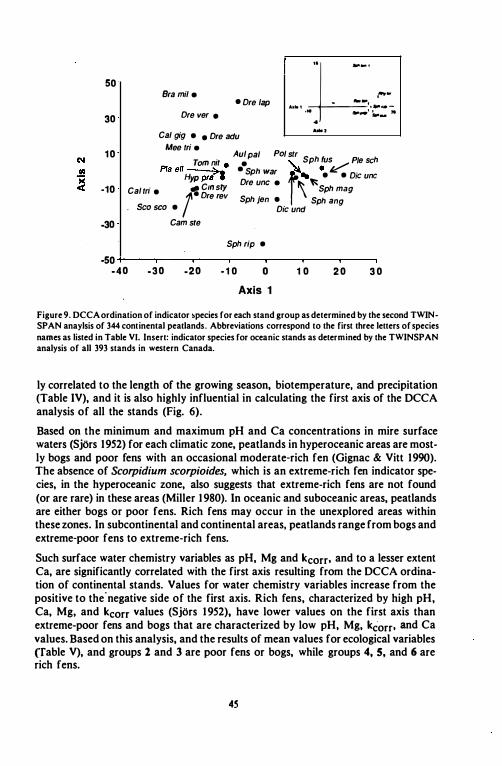
Figure 9. DCCA ordination of indicator .pecies for each stand group as determined by the second TWIN­SPAN anaylsis of 344 continental peatlands. Abbreviations correspond to the first three letters of species names as listed in Table VI. Insert: indicator species for oceanic stands as determined by the TWINSPAN analysis of all 393 stands in western Canada.

ly correlated to the length of the growing season, biotemperature, and precipitation (Table IV), and it is also highly influential in calculating the first axis of the DCCA analysis of all the stands (Fig. 6).

Based on the minimum and maximum pH and Ca concentrations in mire surface waters (Sjors 1952) for each climatic zone, peatlands in hyperoceanic areas are most­ly bogs and poor fens with an occasional moderate-rich fen (Gignac & Vitt 1990). The absence of Scorpidium scorpioides. which is an extreme-rich fen indicator spe· cies, in the hyperoceanic zone, also suggests that extreme-rich fens are not found (or are rare) in these areas (Miller 1 980). In oceanic and suboceanic areas, peatlands are either bogs or poor fens. Rich fens may occur in the unexplored areas within these zones. In subcontinental and continental areas, peatlands range from bogs and extreme-poor fens to extreme-rich fens.

Such surface water chemistry variables as pH, Mg and kcorr, and to a lesser extent Ca, are significantly correlated with the first axis resulting from the DCCA ordina­tion of continental stands. Values for water chemistry variables increase from the positive to the"negative side of the first axis. Rich fens, characterized by high pH, Ca, Mg, and kcorr values (Sjors 1 952), have lower values on the first axis than extreme-poor fens and bogs that are characterized by low pH, Mg, kc"orr, and Ca values. Based on this analysis, and the results of mean values for ecological variables (fable V), and groups 2 and 3 are poor fens or bogs, while groups 4, S, and 6 are rich fens.

4S

Variation in stand position along the second axis resulting from the DCCA analysis of the continental stands is highly correlated with the height above the water surface (Fig. 8). Stand position along this gradient is determined by a line drawn at right angle between the DCCA ordination of that point and the line indicating the height above the water surface (ter Braak 1 987). Based on this analysis. and the mean height above the water surface measurements for each stand group (Table V). stands in group 6 are found closest to the water table. Stands in group 5 occupy the next highest position followed by stands in groups 2 and 4. Stands in group 3 occupy the highest position along the height above the water level gradient. Stand group 1 is found at approximately the same height as groups 2 and4 (Table V).

Stand Groups

Stands in group 1 are separated from stands in group a by the first division resulting from the TWINSPAN analysis of all the stands. This group is found exclusively on the positive side of the first DCCA axis which corresponds to hyperoceanic. oceanic. and suboceanic peatlands (Fig. 6). These oceanic peatlands range from bogs and extreme-poor fens to moderate-rich fens. Stands in group a are found on the nega­tive side of the first axis and are located in subcontinental and continental areas.

Further analyses of these continental stands indicate that stand group 6 is separated from mthe remaining groups by the first division of the TWINSPAN analysis for continental sites. Stands in this group have high pH. kcorr, Ca, and Mg values that are associated with extreme-rich fens, and are found close to the water surface. Stand group 5 is separated from the remaining sites by the second TWINSPAN divi­sion. Stands in this group have slightly lower values for pH, kcorr, Ca, and Mg when compared to those in group 6. On the height above the water surface gradient, stands in group 5 are intermediate between stands in groups 6 and 4. Thus. group 5 contains moderate-rich fens and the second TWINSPAN division separates them from stand groups 2, 3, and 4 that are either drier or have lower pH, kcorr• Ca, and Mg values. The most abundant species in stand groups, 2, 3, and 4 are Sphag­num species while for stand groups 5 and 6 they are brown mosses (Table VI).

Stands in group 2 are separated from those in groups 3 and 4 by the third TWIN­SPAN division. Stands in this group have low pH. kcorr• Ca. and Mg values that are associated with poor fens. On the height above the water surface gradient, these stands are found at approximately the same mean height as stands in group 4 but, more detailed analysis of the standard deviation about the mean (Table V) and DCCA positions reveal that several stands in group 2 are found closer to the water surface than any stand in group 4. Thus, stand group 2 contains wet poor fens and the third TWINSPAN division separates this stand group from the sligtly drier stand group 4 and the much drier stand group 3. Stands in group 3 are distinguished from those in group 4 by the fourth TWIN­SPAN division. Stands in group 3 have lower pH, kcorr, Ca, and Mg values than those in group 4 and could be considered poor fens. However. stands in this group have a wider distribution along the first DCCA axis than those in stand group 2 (Fig.

41l

8). The majority stands in group 3 have lower pH, kcorr, Ca, and Mg values than those in stand group 2 and these are bogs and extreme-poor fens. Stands in group 4 have relatively high pH, kcorr, Ca, and Mg values and are rich fens. The fourth TWINSPAN dividion has thus separated dry rich fens from dry poor fens and bogs.

Indicator species

Hyperoceanic, oceanic, and suboceanic mires

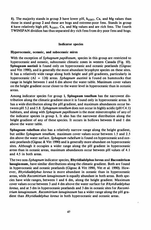
With the exception of Sphagnum papil/osum, species in this group are restricted to hyperoceanic and oceanic, suboceanic climatic zones in western Canada (Fig. 10). Sphagnum austinii is found only on hyperoceanic and oceanic peatlands (Gignac and Vitt 1 990), and is generally the most abundant bryophyte species on these sites. It has a relatively wide range along both height and pH gradients, particularly in hyperoceanic (AI = 1 26) areas. Sphagnum austinii is found on hummocks that range in height between 1 and 6 dm above the water table. Maximum cover values on the height gradient occur closer to the water level in hyperoceanic than in oceanic areas.

Among indicator species for group I, Sphagnum tenellum has the narrowest dis­tribution along the climatic gradient since it is found only in hyperoceanic areas. It has a wide distribution along the pH gradient, and maximum abundances occur be­tween pH 5.2 and 5.8. Sphagnum tenellum does not occur in highly acidic (pH <4. 1) habitats, and along with Sphagnum papillosum i s the most minerotrophic of any of the indicator species in group 1. It also has the narrowest distribution along the height gradient of any of these species. It occurs in hollows between 0 and 1 dm above the water table.

Sphagnum rubellum also has a relatively narrow range along the height gradient, but unlike Sphagnum tenel/um, maximum cover values occur between 1 .5 and 2.5 dm above the water surface. Sphagnum rubel/um is found on hyperoceanic and oce­anic peatlands (Gignac & Vitt 1990) and is generally more abundant on hyperoceanic sites. Although it occupies a wider range along the pH gradient in hyperoceanic areas than in oceanic areas, maximum abundances occur between pH values of 4. 1 and 4.5 in both areas.

The two non-Sphagnum indicator species, Rhytidiadelphus loreus and Racomltrium lanuginosum, have similar distributions along the climatic gradient. Both are found in hyperoceanic and oceanic peatlands (Gignac & Vilt 1990, Vitt et a!. 1990). How­ever, Rhytidiadelphus loreus is more abundant in oceanic than in hyperoceanic areas, while Racom;tr;um lanuginosum is equally abundant in both areas. Both spe­cies have wide ranges, between 1 and 6 dm, along the height gradient. Maximum cover values occur between 3 and 4 dm above the water surface for R hyt;diadelphus loreus, and at 5 dm in hyperoceanic peatlands and 3 dm in oceanic sites for Racom;­tr;um lanuginosum. Racomitrium lanuginosum has a wider range along the pH gra­dient than Rhytidiadelphus loreus in both hyperoceanic and oceanic areas.

47

Sphagnum papillosum has the widest distribution among indicator species for group 1 along the climatic gradient. It is found in both suboceanic and subcontinental areas where none of the other species occurs. Its maximum abundance occurs in hyperoceanic (AI = 126) peatlands where it is the second most abundant species. Maximum abundances are approximately the same in oceanic, suboceanic (AI =

72), and subcontinental (AI = 45) areas. Sphagnum papillosum has a narrow height range, with maximum abundance values occurring between 2 and 3 dm above the water surface in all climatic zones. In hyperoceanic areas, pH values range from 3.4 to 6.7, and maximum cover occurs between 5.6 and 6.3. In oceanic, suboceanic, and subcontinental areas it has a much narrower range along the pH gradient and maxi­mum cover values occur between 4 . 1 and 5.2.

Continental peatlands

Aulacomnium palustre is the only indicator species that is common to almost all continental peatlands regardless of their water chemistry and depth to the water table. It is found in all climatic zones, but is most abundant in subcontinental (AI

= 45) and continental (AI = 27) areas, and relatively rare in the hyperoceanic (AI = 1 26) climatic zone. Abundances increase along both pH and height gradients as the aridity index decreases from hyperoceanic (AI = 1 26) to subcontinental areas. Response surfaces are almost identical for both subcontinental and continental cli­matic zones. In all climatic zones, cover values are relatively small at both low pH and low height values. Maximum cover values occur at pH 5.6 in the oceanic, sub­oceanic (AI = 72) zone, and between 6.3 and 7 .0 in the subcontinental and conti­nental zones. With the exception of the hyperoceanic zone, maximum abundance values are found between 2 and 3 dm along the height gradient.

Continental neutral and acidic fens

Sphagnum warnstorfii is the only indicator species for these fens. It is found in all climatic zones, but m�ximum cover values are found in the subcontinental (AI =

45) and continental (AI = 27) climatic zones. This species' range and maximum abundance along the pH gradient increase with decreasing aridity index values, par­ticularly between hyperoceanic (AI = 1 26) and subcontinental areas. With the ex­ception of oceanic, suboceanic areas (AI = 72), maximum cover values along the height gradient are found at 2 dm above the surface. In oceanic, suboceanic areas, maximum abundances are found at 1 dm above the water surface.

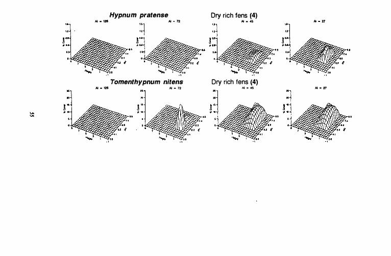
Figure 10. Species response surfaces for 31 indicator species of six stand groups along height above the water surface (dm) and pH gradients for four ccoclimatic regions of western Canada. AI = aridity index. Hypcroceanic: AI = 126; oceanic, suboceanic: AI = 72; subcontinental: AI = 4S; Continental: AI =

27 - from left to right. Sec Figs. 6-8 for delimits of stand groups.

48

"

�

!

Rhytidladelphus loreus AI - 128 AJ • 72

Sphagnum papil/osum N - � N - n

r -

. .

Oceanic fens and bogs ( 1 )

" N - 45 N - 27

"

... ..

Oceanic fens and bogs ( 1 ) N - 45 N - 27

..

Oceanic fens and bogs ( 1 ) AI - 45 N - 27

t

'Jo :::>

..

r ' . .. os

"

! •

AI . ,"

AI • 126

Sphagnum austin;; AI .. 72

'"

f'

Sphagnum tenellum AI '" 72

! . • I

..

Sphagnum rubel/um AI - 72

Oceanic fens and bogs (1 ) AI .. 4S AI .. 27

"J "' , :J ! "

Oceanic fens and bogs (1 ) AI .. 4S AI .. 27

"

I. ..

Oceanic fens and bogs (1 ) AI _ <5 "

:

-� � . In ,

...., � � ...., �

- If) <0 c: , � N - .2 If) "0 c: 'Q ·0 � � , CU , 1ij '1 "0 '1 - c: c: CU CI> 1ij c: :;:: .... -c: :l 0 . CI> () • Z ...., � ...., �

� � .-� 7 :;: - ... /I) '1 Q ;:, -- /I) as E Q.

E � � • . E c: E ...., � ;:, ...., �

Q c: u 01 .s as .c: ;:, � q:

� � , , '1 '1

51

IA ....

50 ..

r " _ ..

.. ..

r " . ..

Sphagnum magellanicum Sphagnum-dom. fens and bogs (2-4)

N . l28

AI • 72

.. j " i !" # 1O� .... �� # 10

AI • 45

...... Sphagnum angustifolium Sphagnum-dom. fens and bogs (2-4)

AI - n AI - 45 50

.. ..

f O . .. !

• f O . ..

" u

'0 ...... .,

Sphagnum fuscum Sphagnum-dom. fens and bogs (2-4) AI - 126 AI - n AI - 45 50

.. ..

! •

... .. ...

AI • 27

AI _ 27

...

� •

r'� IA . .. .... ! :j

Sphagnum rlparium Wet poor fens (2) fJ,J - 126 N - 72 AI • 45

"

� •

Sphagnum jensen Ii Wet poor fens (2) N - 126 N - 72 AI _ 45 2$-

,.

�� . . ! :1 � !:.

>---- 1$ S . .

, , . j .

. ,

Pleurozium schreberi M _ 126 N - 72

"'1 .. �/?r_ � :J �//h'

...... Dry poor fens and bogs (3)

"'1

C]

Ad _ 45

:7j,&'W/A .'1.. .A.... ... .

"'1

! " n .

N - 27

/IJ · 27

/IJ • 27

v. �

j •

j •

& •

� - 128

Po/ytr/chum strictum AI :III 72

"

! . • •

Dlcranum undulatum N - n

! . · ,

..

" I " �

! . . ,

Drepanocladus unclnatus N - n

j ! • •

Dry fens (3-4) AI '" 45 AJ • 27 " ,

"

.i • · .

Dry fens (3-4) AI - 45 N • 27

! ' · ,

�x�u ..

Dry fens (3-4) AJ - 45 AJ - %7

j •

""

.... ....

Hypnum pratense Dry rich fens (4) N · � N - n N . �

j � r] � J0'" � J � o.� �_ .. 0 � '#U� � .,.

l •

'"

Tomenthypnum nitens 14 - 128 f:iJ - 72 os

j " . ..

Dry rich fens (4) AI • 45 ..

..

.. ..

N - 1:7 .. ..

..

Drepanocladus aduncus Moderate-rich fens (5) fIJ • 128 AI • 72 /OJ - ..

j ' . , r . , .. ..

•

h.p,,' , Brachythecium mildeanum Moderate-rich

-'fens (5)

AI • 126 AI • 72 AI - 45 AI _ 27

j ' g:

...... Drepanocladus polycarpus

H · 126 Moderate-rich fens (5)

/OJ _ v

! • !

•

'" ......

! . . .

! •

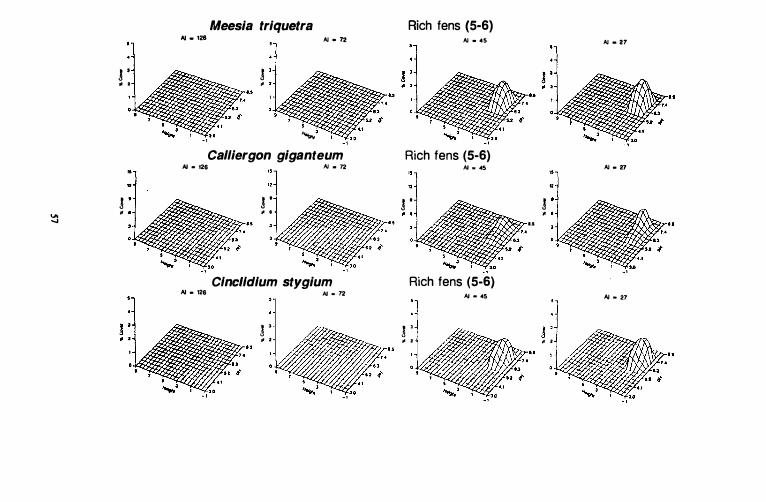
AI . 128 Meesia triquetra

AI - n

! ·

"­Call1ergon giganteum

AI - 126 AJ _ 72

! . · .

Clnclldlum stygium AI • 126 AI · n

! ' · .

Rich fens (5-6) AI _ 45 AI - 27

Rich fens (5-6) AI . 45 AI _ 27

"

! . ! •

.. ..

Rich fens (5-6) AJ - 45 AI - 27

! 3 . . . .

'" 00 � •

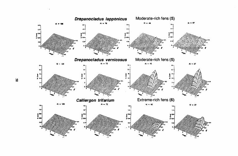
, . AI - 126

..

Drepanocladus lapponicus " AI _ no "

"

Drepanocladus vernicosus AI _ 72 " "

"

! . • •

..

Call1ergon trlfar/um

..

Moderate-rich fens (5) AI • •• AI _ .,

Moderate-rich fens (5) AI = 45 AI - 27

u

Extreme-rich fens (6)

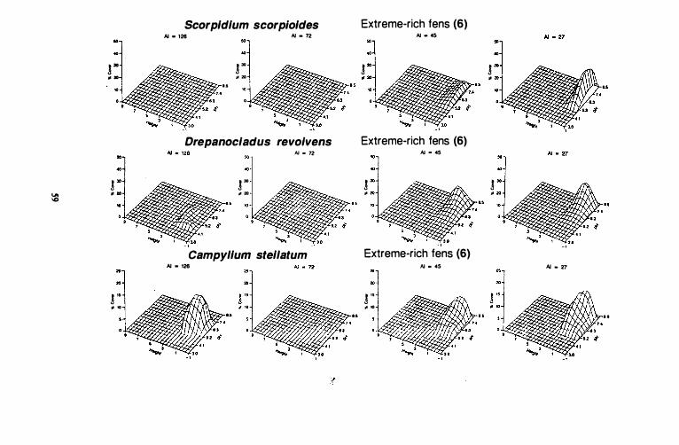
Scorpldlum scorpioldes Extreme-rich fens (6) AJ - 126 AJ - 72 AJ - OS

50

� ,. ! " ! ! . .. . .. • • .. ..

Drepanocladus revolvens Extreme-rich fens (6) AI - 72 AI - 45

..

! ! " ! ! � • . .. . .

...... .. Campy/lum stel/atum Extreme-rich fens (6)

JI,J - 128 ,. AI _ 45 AJ - V

..

! " ! " . .. . .. I t

Continental Sphagnum-dominated fens and bogs Abundance values for Sphagnum magellanicum are highest in the oceanic, suboce­anic zone (AI = 72). This species has a relatively narrow range on the pH gradient that extends from pH 3.4 to 5.6 and maximum abundances occur at pH 4. 1 in all climatic zones. On the height gradient, Sphagnum magellanicum is found between 1 and 5 dm. With the exception of the oceanic, suboceanic zone, maximum abun­dances are found between 2 and 3 dm above the water surface. Although it has a wide range along this gradient, cover values are greater at heights above 3 dm when compared to abundances at lower heights. With the exception of the oceanic, sub­oceanic zone, there appears to be no difference in its distribution along the height and pH gradients between climatic zones.

Although Sphagnum angustifolium is slightly more abundant in, oceanic (AI =

1 26) areas and slightly less abundant in oceanic, suboceanic ones (AI = 72), it shows little climatic preference. Its distribution ranges between pH 3.0 and 6.7 and it has the most acidic range among indicator species for this group. Maximum abundance occurs between pH 4.1 and 4.5 in all climatic zones with the exception of the oceanic one (AI = 126) where it reaches maximum abundance at pH 4.8. Sphagnum angu­stifolium also has the narrowest range on the height gradient among indicator spe­cies for this group. It is found between 0 and 4.5 dm above the water surface and, with the exception of the hyperoceanic zone, it maximum cover occurs relatively close to the water surface at approximately 2 dm in all climatic zones. In the hyper­oceanic areas, maximum abundance occurs at approximately 4 dm above the water table.

Sphagnum fuscum is the most abundant species among those in this group. Al­though it is abundant in all climatic zones, it reaches its maximum cover in subconti­nental (AI = 45) areas. It occurs on peatlands that have pHs ranging between 3.4 and 7.4, but, it is not as abundant on peatlands having high pH values (>5.2) in hyperoceanic (AI = 1 26) and oceanic, suboceanic (AI = 72) areas. As is the case for Sphagnum angustifolium, S. fuscum has a bimodal distribution on the pH gra­dient. The distribution of S. fuscum along the height gradient is between 1 and 7 dm above the surface of the water, however, it has a relatively narrow distribution along this gradient in hyperoceanic peatlands (AI = 1 26). Its maximum cover on the height gradient appears to be' negatively correlated with the climatic gradient. The height above the water table at which the maximum cover values occur increases as the aridity index decreases. At low heights above the water table, the abundance of S, fuscum is negatively correlated with the pH gradient.

Continental dry fens and bogs

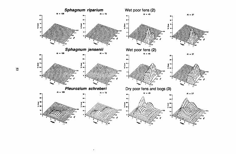
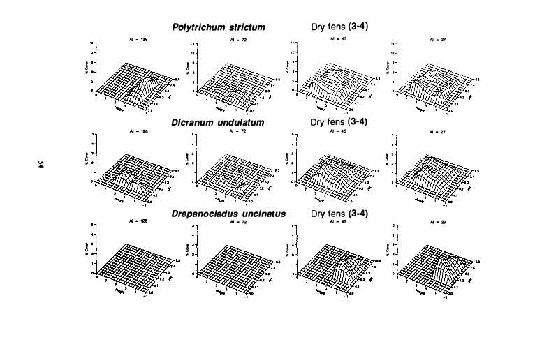
Polytrichum strictum is found in all climatic zones but is much less abundant in oce­anic, suboceanic areas (AI = 72). This species reaches its maximum cover on sub­continental (AI = 45) and continental sites (AI = 27). Polytrichum strictum occurs over a broad pH range however, it achieves its maximum cover between pH 3.4 and 5.6. In oceanic, suboceanic areas, it is not abundant at higher pH values (>5.2).

60

Although P. strictum occupies a wide range on the height gradient in continental and subcontinental peatlands, it has a relatively narrow range in oceanic areas (AI>72). Maximum cover values for this species on the height gradient are relative­ly close to the water surface (2 dm) on hyperoceanic (AI = 1 26) and oceanic, sub­oceanic peatlands when compared to subcontinental and continental sites 4 to 6 dm). In all climatic zones, the abundance of P. strictum decreases at lower heights as pH values increase above 5.3. Dicranum undulatum is also found in all climatic zones in western Canada but is more abundant in continental (AI;S45) than in oceanic (AI>45) areas. Maximum abundances for Dicranum undulatum are slightly greater in subcontinental (AI =

45) than continental (AI = 27) areas. Although it is found over a wide range along the pH gradient, it is more abundant at pH values less than 5.6. Its range along the pH gradient gradual\y increases from hyperoceanic (AI = 1 26) to subcontinental areas. However, maximum cover values occur between pH 4.4 and 4.8 in al\ climatic zones. Response surfaces are bimodal along the pH gradient in the subcontinental and continental zones. Heights above the water surface range from I to 6 dm in al\ climatic zones. Maximum abundances along the height gradient increase from hype­roceanic to subcontinental areas. With the exception of slight differences in maxi­mum abundances', response surfaces in subcontinental and continental areas are al­most identical.

Drepanoc\auds uncinatus is only found on subcontinental (AI = 45) and continen­tal (AI = 27) peatlands in western Canada, and cover values are slightly higher in continental areas. pH values for this species range between 4.4 and 7.4 and it has a bimodal distribution along this gradient. Maximum abundances for D. uncinatus are found at 5 .2 on the pH gradient and at 2 dm above the water table.

Continental moderate- and extreme-rich fens

Neither Calliergon giganteum nor Meesia triquetra is found on peatlands in hypero­ceanic, oceanic, and suboceanic zones (AI >72). Both species occupy approximately the same ranges along the pH and height gradients, and neither is very abundant in peatlands on which they are found. Calliergon giganteum has a skewed distribu­tion along the pH gradient, and it is more abundant at high values. Meesia triquetra also has a slightly skewed distribution and is more abundant at higher pH values. Differences between these two species along the pH gradient are that Calliergon gi­ganteum is abundant at pH 7 .8 while Meesia triquetra is not. Meesia triquetra achieves its maximum abundance between 0 and 0.5 dm above the water surface, while Calliergon giganteum is most abundant between 1 and 1 .5 dm.

Cinclidium stygium can be found between pH 5.6 and 7.8 with maximum cover val­ues occurring between 6.3 and 7.8. This species has a relatively wide range along the height gradient and can be found between 0 and 3 dm. Maximum cover values along this gradient change depending on the pH. At pH values less than 6.7, maxi­mum abundances occur between 1 and 3 dm above the water surface. At high pH values (>6.7), maximum cover values are found closer to the water surface, be­tween 0 and I dm.

61

Continental wet poor fens

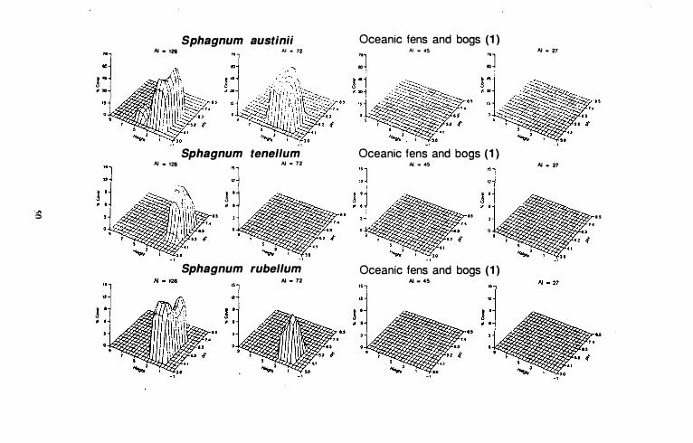
Response surfaces for Sphagnum riparium are almost identical in both subcontinen­tal and continental areas. Sphagnum riparium has a relatively narrow range along the pH gradient that does not extend beyond 5 .6, and maximum cover values occur below pH 4. I . Maximum abundances for Sphagnum riparium also occur at the sur­face of the water, but it is not abundant below the surface. Sphagnum jensenii has the highest abundance values among indicator speCies in this group. As with Sphagnum riparium, response surfaces for this species are almost identical in subcontinental and continental areas. It has a relatively wide range on the pH gradient, between 3.0 and 6.7 and maximum abundances occur between 5 . 2 and 6.0. O n the height gradient, Sphagnum jensenii i s located between -1 and 3 dm above the water surface. Maximum abundances are found at the surface of the wa­ter surface.

Continental dry poor fens and bogs

Pleurozium schreberi is much less abundant in hyperoceanic (AI = 1 26) and ocean­ic, suboceanic (AI = 72) peatlands than on subcontinental (AI = 45) and continen­tal (AI = 27) sites in western Canada. This species occurs in peatlands having pH values ranging from 3.4 to 8. 1 in all climatic zones but i t is not very abundant at high pH values (>5.2) in hyperoceanic areas. Pleurozium schreberi is found be­tween I and 7 dm above the water table at low pH values in all climatic zones. At higher pH values, heights above the water surface at which it is found gradually in­crease from hyperoceanic areas to continental areas. It achieves its maximum abun­dance at 6 dm above the water surface and between pH 6.3 and 7.4. At heights less than 3 dm, its abundance is negatively correlated with the pH gradient in all climatic zones. Cover values steadily decrease as pH increases from 4.1 to 7.4.

Continental dry rich fens

Tomenthypnum nitens has the highest abundance values among indicator species in group 4. It is found in all climatic zones with the exception of the hyperoceanic zone. pH values range between 4.5 and 7.8 in all climatic zones. However, maxi­mum abundances occur at pH 5.6 in oceanic, suboceanic (AI = 72) areas, while they are found between 5.8 and 7.4 in subcontinental (AI = 45) and continental (AI =

27) areas. Response surface dimensions along the height gradient are slightly nar­rower in the oceanic, suboceanic climatic zone, than in other zones. Maximum abundances are found at 2 dm above the surface of the water in all climatic zones.

Abundances for Hypnum pratense are much lower than those for Tomenthypnum nitens. Unlike Tomenthypnum nitens it is only found in continental and subconti­nental and it is more abundant in continental than subcontinental areas. It is found between pH 4.8 and 7.0 and maximum cover values along the pH gradient occur between pH 5.6 and 6.3. Maximum values along the height gradient are found be­tween 1 and 2 dm above the water surface.

62

Continental moderate-rich fens

With the exception of Drepanocladus aduncus, indicator species for this group are only found on carpets and lawns between 0 and 3 dm above the surface of the water table and do not occur in oceanic areas (AI >72). Also, with the exceptions of Dre­panocladus aduncus and Drepanocladus vernicosus, species ranges along the pH gradient are narrow. Drepanocladus ad uncus is the only group 5 indicator that is found in the oceanic, suboceanic climatic zone (AI = 72). It is also the only species that is more abundant in subcontinental (AI = 45) areas than in continental (AI = 27) areas. pH values for this species range betwen 5.0 to 7.4. Maximum cover values occur at pH 6.0 in the oceanic, suboceanic climatic zone and at pH 6.7 in other areas. Drepanocladus aduncus is found between -I and 3 dm along the height gradient and is the only spe­cies that is abundant below the surface of the water. However, maximum abun­dances are found between I and 2 dm above the water surface. Although Brachythecium mildeanum is found in both subcontinental (AI = 45) and continental (AI = 27) areas it is more abundant in the latter. It has a narrow pH range, between 6.0 and 7 .8, and maximum abundances in both climatic zones occur between pH 7.0 and 7.4. Brachythecium mildeanum also has narrow range along the height gradient, with maximum cover values occurring between I and 2 dm. Drepanocladus polycarpus is less abundant in subcontinental (AI = 45) than in con­tinental (AI = 27) areas. However, ranges for response surfaces along pH and height gradients are the same in both climatic zones. This species is found between pH 6.3 and 7.4, and maximum cover values occur between 7.0 and 7.4. Along the height gradient, Drepanocladus po!ycarpus is found between I and 3 dm, and maxi­mum abundances are at 2 dm. Drepanocladus lapponicus has almost identical response surfaces in both subconti­nental and continental areas. It also has the lowest abudances values and the nar­rowest response surface dimensions along both height and pH gradients among indi­cator species for 5. It is found between pH 6.0 and 7.0 and maximum abundances occur between pH 6.6 an 7.0. Along the height gradient it is found between 0 and I dm. Drepanocladus vernicosus is slightly more abundant in continental (AI = 27) than in subcontinental (AI = 45) areas. Response surface dimensions for both climatic zones are similar. This species has a relatively wide pH range compared to other in­dicator species in group 5, with values ranging between 5.2 and 7.4. However, this species is less abundant at lower pH values within its range and maximum cover val­ues are found between pH 6.6 and 7.4. Along the height gradient, Drepanocladus vernicosus is found between I and 3 dm above the water surface. Maximum cover values occur between I and 2 dm above the water surface.

Continental wet extreme-rich fens

Group 6 indicator species can all be found below the surface of the water table and are only found in subcontinental (AI = 45) and continental (AI = 27) peatlands.

63

J\.UllUUgU dU .)Vl.\..U •• .) dH ! ,ihJi \.. dUUUU41U.L J.H \,.uU. ... U1\ ... J,u" .u. ""h .. ","') UJ.cUl hi 4Uy ()lU�l �11-matic zones, the shape of the response surfaces are very similar for both continental and sub-continental areas.

Among species in group 6, Calliergon trifarium has the lowest abundances. It has a relatively narrow range along the pH gradient and is found between pH 5 .6 and 7.4. Maximum abundances are found between pH 6.6 and 7.0. It can be found be­tween -\ and 2 dm along the height gradient but is most often found at the surface of the water.

Scorpidium scorpioides has a wide range along the height gradient and can be found between pH 5.2 and 8.5. Maximum cover values occur between 7.4 and 8. 1 . Scorpi­dium scorpioides is the only species among indicators for group 6 that is more abun­dant below the surface of the water than above. Maximum cover values occur be­tween 0 and - I dm and abundances rapidly decrease above the surface of the water.

Drepanocladus revolvens is found in all climatic zones but is not abundant in ocean­ic areas (AI = 72).Drepanocladus revolvens is found on peatlands having surface water pH values between 4.5 and 8 . 1 , but it is only found at low pH values « 5.2) in t he hyperoceanic zone. Apart from hyperoceanic areas, maximum abundances are found between pH 7.4 and 8 . 1 . Height values range between -I and 2 dm and maximum abundances are found between 0 and I dm.

Along with Drepanocladus revolvens, Campylium stellatum is found in all climatice zones, but abundances are relatively low in the hyperoceanic areas (AI = 1 26), and even lower in the oceanic, suboceanic zone (AI = 72). This species has its widest distribution along the pH gradient in subcontinental and continental areas and its maximum abundances are found at high pH values (>7.8). Campylium stel/atum occurs between -I and 2.5 dm relative to the surface of the water and can occasional­ly be found below -1 dm in subcontinental and continental areas. Maximum abun­dances however are found between the surface of the water and I dm. At low height abundances increase with increasing pH .

Summary

Bryophyte species that occur in mires in western Canada clearly respond to gradients of climate, surface water chemistry, and height above the water surface. Several di­stinctive habitat patterns are present for the indicator species selceted in this study.

Species of oceanic fens and bogs generally occur at greater heights above the water level as the climate changes from oceanic to hyperoceanic. This trend can be easily seen in the response surfaces for Racomitrium lanuginosum and to a lesser extent for Sphagnllm austinii. Both S. rubel/um and S. austinii occur at higher pH's as aridity decreases. Whereas the response of Sphagnum papil/osum to height remains fairly constant over the climatic gradient, its response to pH is markedly different in hyperoceanic climates when compared to oceanic and subcontinental climates.

Widespread species such as Aulacomnium palustre and Sphagnum warnstorJii are

64

l;I,;Ul,;ldUj I,;UIIIlUU,1 W1 UUglluul l,,� MUUY ilU;a, llUweVCJ lilt: aUUlluaJlt:e 01 both 01 these species is clearly greatest in continental rich fens. Both species occur higher above the water surface in continental areas than they to in oceanic and hyperocean­ic areas, perhaps due to increased competition from other species of bryophytes in the latter areas. Likewise, both of these species are more common in rich fens than in poor fens and bogs, especially S. warnstorfii that is able to tolerate higher alkali­nities than other sphagna.

Although Sphagnum mage/lanicum, S. angustifolium, and S. fuscum all occur throughout the climatic zones of western Canada, these three species are a much more prevalent component in suboceanic, subcontinental, and continental mires than in oceanic and hyperoceanic areas. Sphagnum mage/lanicum is much more re­stricted to lower pH's than are either S. angustifolium or S. fuscum. Both of these latter two species have bimodal distributions, and occur higher above the water sur­face in rich fens than in poor fens. The bimodal distributions are present due to the fewer number of peatlands having pH's around pH 5.5. Sphagnum angustijolium is able to occur higher above the water surface in hyperoceanic mires than in more continental ones. Sphagnum fuscum is more restricted in its occurrence in hyper­oceanic and oceanic areas and only becomes the dominant hummock species in sub­continental and continental conditions, where such oceanic species as S. austinii are lacking. Polytrichum strictum and Dicranum undulatum have similar response sur­faces. Both species are more abundant and widespread in continental mires than in oceanic and hyperocanic ones. In this regard, both species follow the responses of Sphagnumfuscum closely, occurring on relatively high (and dry) hummocks. Dicra­num undulatum is more abundant in rich fens, while Polytrichum strictum is more common in poor fens and bogs. Although Drepanoc/adus uncinatus is a widespread species of temperate and boreal upland forests, in continental and subcontinental areas it also occurs in rich fens and poor fens as well as in bogs. According to our data, it does not occur (or is very rare) in mires in oceanic and hyperoceanic areas, there largely replaced by such mosses as Rhytidiadelphus lorells.

Large, continental poor fens, often patterned, are characterized by Sphagnum ripa­rium and S. jensenii. Both of these carpet species have similar response surfaces; S. riparium is more restricted in its pH response, while S. jensenii is more abundant at higher pH's and in somewhat deeper water. Neither of these species occurs in oce­anic or hyperoceanic climatic zones, there replaced by S. tenellllln and other sphag­na (e.g.: S. lindbergii, S. pacificum and S. mendocinum).

In dry, forested peatlands of continental Canada, Pleurozium schreberi can become a dominant species. Although common in bogs and poor fens, it is largely excluded from the highest and driest hummocks in these mires, probably due to the abun­dance of Sphagnum fuscum (and S. nemoreum), while in rich fens it reaches its highest abundance on dry hummocks. In hyperoceanic and oceanic areas, its abun­dance is greatly reduced, there replaced mostly by a variety of Sphagnum species and by Racomitrium lanuginosum. On the driest hummocks in continental bogs, Pleurozium, along with species of Cladina, are often dominant, however these dry hummocks are not present in hyperoceanic areas, where the hummock tops are usually dominated by species of Sphagnum, particularly S. austinii and S. rubel/um.

65

Whereas nch lens are the mOSl common nllre lype 111 SUbcolll1llelltal allu cont1l1ental western Canada, in hyperoceanic and oceanic regions of Canada these mire types are rare. As a result, bryophyte species that are abundant in rich fens are either ab­sent, rare, or if present then not abundant in oceanic areas of.the continent. Hyp­num pratense is a rare species of lawns and hummock sides, restricted to rich fens in subcontinental and continental areas. Although much more restricted in distribu­tion, its response suc;'ace is somewhat similar to that of Tomenthypnum nitens, which is the predominant hummock-forming species of rich fens. The change in re­sponse of this specks to pH between subcontinental and suboceanic-oceanic cli­mates is probably due to the lack of habitats at the higher pH's in these latter cli­mates. Species of bryophytes that are characteristic of rich fens consistently occur only above pH's of 5.5 . Species with broad responses to pH such as Meesia trique­tra, Calliergon giganteum and Cinciidium stygium are largely restricted to subconti­nental and continental climates. These species can be abundant in both moderate­and extreme-rich fens, although they are normally more abundant in mires with the higher pH's. Cinc/idium stygium becomes more abundant at lower heights as pH incrases, suggesting that it is more tolerant of higher pH's.

Species that occur in moderate-rich fens become more common as aridity increases. These species all appear to be tolerant of fluctuating water leveis and have been shown to tolerate higher nutrient levels than species of extreme-rich fens (Vitt & Chee 1 99 1 ). All of these species have response surfaces limited to pH's of less than 7.4 and greater than about 5.2. Drapanociadus aduncus and D. /apponicus both oc­cur submerged or emergent (or higher in the former species), while D. vernicosus and D. polycarpus are more abundant at somewhat drier habitats. These four spe­cies can be considered as two species pairs; D. aduncus occurring submerged and in emergent carpets replaced by D. polycarpus in drier (and higher) sites and similar­ly for D. lapponicus being replaced by the more drought tolerant D. vernicosus.

Wet extreme-rich fens are clearly characterized by Scorpidium scorpioides, Callier­gon trijarium, Drepanociadus revolvens, and Campylium stellatum. Whereas all of these species can occur at pH's as low as 5.2, they all extend into habitats with pH's above 7.4. Differences in tolerance to height above the water surface is clearly shown by the response surfaces of Scorpidium scorpioides, Drepanoc/adus revol­vens, and Campylium stellatum.

Bryophytes are among the best indicators of mire types along climatic, chemical, and physical gradients. Species responses to these important gradients can be quan­tified and used to characterize the habitat preferences of critical indicator species. The marked differerences in responses to pH and height gradients when compared over the climatic gradient present in western Canada strengthens the view that cli­mate often has an over-riding effect on the distribution of bryophyte species and that species may respond to chemical and physical gradients differently under diffe­rent climatic regimes. These individualistic responses can be used to inter individual species as well as general vegetation responses to climatic changes, both past and present.

66

Acknowledgments

We wish to thank W.L. Chee, D.G. Horton, J.D. Johnson, H.J. Kubiw, B.J. Nicholson, and L. Roche· fon for being able to use their data sets. This project was funded by a Strategic Grand from the Natural Sciences and Enginering Research Council of Canada (NSERC) to S.E. Bayley, D.H. Vitt and D.W. Schindler. Data sets of D.H. Vitt were obtained from research suppon largely by NSERC operating grant A6390, for which we are grateful.

literature cited

ADAMS, G.D. (1988): Wetlands of the prairies of Canada. pp. 157-198. - In: Wetlands of Canada. Na· tional Wetlands Working Group. Ecological Land Classification Series, No. 24. Sustainable Develop· ment Branch, Environment Canada, Ottawa, Ontario and Polyscience Publications Inc., Montreal.

ALLAN, J.A. (1943): Province of Alberta: Geology. - Research Council of Alberla. Report No. 34. Ed· monton, Alberta. 196 p.

ANDRUS, R.E. (1980): Sphagnaceae (Peat moss family) of New York State. 89 pp. - In: Contributions to a Flora of New York State III. R.S. Mitchell (ed.). Bulletin No. 442. New York State Museum.

ANDRUS, R.E., D.J. WAGNER & J.E. TITUS (1983): Vertical zonation of Sphagnum mosses along hummock-hollow gradients. - Canadian J. Bot. 61: 2138-3139.

ANDRUS, R.E. (1987): Nomenclatural changes in Sphagnum imbricatum sensu lato. - Bryologist 90: 217-220.

ANONYMOUS. ( 1982a): Canadian climate normals. Temperature and precipitation 195 1 -1980 British Columbia. A publication of the Canadian Climate Program MDC: 551-582 (7 1 1). 268 p.

ANONYMOUS. ( 1982b): Canadian climate normals, Vol. 3. Precipitation 1951- 1980. A publication of the Canadian Climate Program MDC: 551-582. 602 p.

ANONYMOUS. 1986. Climate of Alberta. Tables of temperature, precipitation and sunshine. Report 1986. Alberta Environment. 84 p.

BANNER, A., R.J. HEBDA, E.T. OSWALD, J. POJAR, & R. TROWBRIDGE (1988): Wetlands of Pacific Canada, pp. 308-346. In: Wetlands of Canada. National Wetlands Working Group. Ecological Land Classification Series, No. 24. Sustainable Development Branch, Environment Canada, Ottawa, Ontario and Polyscience Publications Inc., Montreal.

BANNER, A., J. POJAR & R. TROWBRIDGE ( 1986): Representative Wetland Types of the Northern Part of the Pacific Ocean Wetland Region, British Columbia". Ministry Forest Research Report RR85008-PR. Victoria.

CHEE, W.L. & D.H. VITI 1990. The vegetation, surface water chemistry and peat chemistry of moderate-rich fens in central Alberta, Canada. - Wetlands 9: 227-26 1 .

CLYMO, R.S. ( 1964): The origin o f acidity i n Sphagnum bogs. - Bryologist 67: 427-43 1 .

CL YMO, R.S. (1967): Control of cation concentrations, and in particular of pH, in Sphagnum domi­nated communities. pp. 273-284. In: H.L. Golterman & R.S. Clymo (eds.). Chemical Environment in the Aquatic Habitat. Proceedings of an International Biological Program Symposium. North Holland Publishing Co. Amsterdam.

CLYMO, R.S. & P.M. HAYWARD (1982): The ecology of Sphagnum. pp. 229-289. In: A.J.E. Smith (ed.). Bryophyte Ecology. Chapman & Hall. London.

CRUM, H. (1988): A focus on peatlands and peat mosses. The University of Michigan Press. Ann Arbor. 306 p.

DAMMAN, A.W.H. (1977): Geographical changes in the vegetation pattern of raised bogs in the Bay of Fundy region of Maine and New Brunswick. - Vegetatio 35: 137-1 5 1 .

67

DAMMAN. A.W.H. ( 1979): Geographical patterns in peatland development in eastern North America, pp. 42-57. In: Kivinen. E., L. Heikurainen, and P. Pakarinen (eds.). Proceedings of the International Symposium on Classification of Peat and Peatlands. Hyytiaill.

DANIELS. R.E. & A. EDDY ( 1985): Handbook of European Sphagna. Institute of Terrestrial Ecology. Natural Environment Research Council. Abbots Ripton, Great Britain. 262 p.

DANSEREAU. P. & F. SEGADAS-VIANNA (1952): Ecological study of the peat bogs of eastern North America . I. Structure and evolution of vegetation. - Canadian J. Bot. 64: 2576-458 1 .

DAUBENMIRE, R .F. (1959): A canopy-coverage method o f vegetation analysis. - Northwest Science 33: 43-64.

D1ERSSEN, K. (1983)� Zur Verbreitung und Soziologie von Sphagnum ,ipa,ium Angstr. in Mitteleuro­pa. - Andria 2: 9-22.

DU RIETZ. G.E. ( 1 949): Huvidenheter och huvidgrllnser i Svensk myrvegetation. Summary: Main units and main limits in Swedish mire vegetation. - Svensk Bot. Tidskr. 43: 274-309.

DU RIETZ. G.E. ( 1954): Die Mineralbodenwasserzeigergrenze als Grundlage einer natarlichen Zweiglie­derung der Nord- und Mitteleuropllischen Moore. - Vetetatio 5-6: 571-585.

ECOREGIONS WORKING GROUP ( 1989): Ecoclimatic Regions of Canada: First Approximation. Ecological and Classification Series, No. 23 , Sustainable Development Branch, Canadian Wildldife Ser­vice. Conservation and Protection. Environment Canada. Ottawa, Canada. 1 19 p.

EUROLA, S. (1962: Ober die regionale Einteilung der sUdfinnischen Moore. - Vanamo 33: 1-243.

FLATBERG. K.l . (1989): Sphagnum (Cuspidata) pacificum, sp. nov. - Bryologist 92: 1 16':1 19.

GAUTHIER, R. (1980): La vegetation des tourbieres et les sphaignes du Pare des Laurentides, Quebec. Etudes .:cologiques No. 3. Laboratoire d'ecologie forestiere, Universite Laval, Quebec.

G IGNAC. L.D. (1987): La distribution des bryophytes sur des tourbieres contaminees par des metaux dans la region de Sudbury, Ontario, Canada. - Cryptogamie, Bryologie Lichenologie 8: 339-35 1 .

GIGNAC, L.D. & D.H. VITI ( 1990): Habitat limitations of Sphagnum along climatic, chemical and physical gradients . . Bryologist 93: 7-22.

G IGNAC, L.D., D.H. VITI, & S.E. BAYLEY (1991): Bryophyte response surfaces along ecological and climatic gradients . . Vegetatio (in press).

GLlME, J .M. ( 1982): Response of Fonlinalis hypnoides to seasonal temperature variation. - J. Hattori Bot. Lab. 53: 1 8 1 · 193.

GORHAM, E. (1956): The ionic composition of some bog and fen waters in the English Lake District. - J. Ecol. 44: 142·152.

GORHAM, E. & W.H. PEARSALL ( 1956): Acidity, specific conductivity and calcium content of some bog and fen waters in northern Britain . . J. Ecol. 44: 129·141 .

GREEN. R. ( 1972): Geological Map of Alberta. Research Council of Alberta. Map 35. Edmonton, Alberta.

HAYWARD, P.M. & R.S. CLYMO ( 1983): The growth of Sphagnum: Experiments .of light flux and water table depth. - J . Ecol. 71: 845-863.

HEMOND, H. (1980): Bicgeochemistry of Thoreau's bog, Concord, Massachusetts. - Ecol. Monographs SO: 507-526.

H I LL, M .O. ( 1979): TWINSPAN - A Fortran program for arranging multivariate data in an ordered two-way table by classification of individuals and attributes. Ecology and Systematics, Cornell Universi­ty, Ithaca.

HOLLAND, S.S. ( 1964): Landforms of British Columbia. A physiographic outline. B.C. Department Mines and Petroleum Resource Bulletin No. 48. Victoria.

68

HORTON, D.G., D.H. VITT, & N.G. SLACK ( 1979): Habitats of circumboreal-subarctic sphagna: I . A quantitative analysis and review of species in the Caribou Mountains, northern Alberta. Canadian J. Bol. 57: 2283-23 17.

IRELAND, R.R., G.R. BRASSARD, W.B. SCHOFIELD, & D.H. VITI (1987): Checklist of the mosses of Canada. II. Lindbergia 13: 1-62.

JANSSENS, J.A. (1983): Past and extant distribution of D,epanocladus in North America, with notes on the differentiation of fossil fragments. - J. Hattori Bot. Lab. 54: 25 1-298 .

. JEGLUM, J.K. (1971): Plant indicators of pH and water level in peatlands at Candle Lake, Saskatche· wan . • Canadian J. Bot. 49: 1661· 1676.

JEGLUM, J.K. (1972): Boreal forest wetlands near Candle Lake, central Saskatchewan . • Musk·ox 1 1 : 4 1 ·58.

JEGLUM, J.K. ( 1973): Boreal forest wetlands near Candle Lake, central Saskatchewan. Part II. Rela· tionships of vegetational variation to major environmental gradients . • Musk·ox 1 1 : 41·58.

JONGMAN, R.H.G., G.J.F. TER BRAAK, & O.F.R. VAN TONGEREN (1987): Data Analysis in Community and Landscape Ecology. Centre for Agricultural Publishing and Documentation. Wagenin· gen, Netherlands. 299 p.

KARLIN, E.F. & L.C. BLISS ( 1984): Variation in substrate chemistry along microtopographical and wa· ter chemistry gradients in peatlands . . Canadian J. Bol. 62: 142·153.

KUBIW, H., M. HICKMAN, & D.H. VITI (1989): The developmental history of peatlands at Muskiki and Marquerite Lakes, Alberta . • Canadian J. Bol. 67: 3534·3544.

MILLER, N.G. ( 1980): Mosses as paleoecologcial indicators of lateglacial terrestrial environments: some North American studies . • Bull. Torrey Bol. Club 107: 373·39 1 .

MOORE, P.D, & D.J. BELLAMY (1974): Peatlands. Springer·Verlag, New York. 222 p.

NICHOLSON, B.J. & D.H. VITI ( l990a): The wetlands of Elk Island National Park, Alberta. Supply and Services Canada. Report No. K3482·8-0122101 SS.

NICHOLSON, B.J. & D.H. VITI ( l990b): The paleoecology of a peat land complex in continental western Canada, • Canadian J. Bol. 68: 121 · 138.

0KLAND, R.H. (1989): A phytoecological study of the mire Northern Kisselbergmosen, SE Norway. I. Introduction, nora vegetation, and ecological conditions . • Sommerfeltia 8: 1· 172.

PAKARINEN, P. (1979): Ecological indicators and species groups of bryophytes in boreal peatlands. pp. 121· 134. IN: Kivinen, E., L. Heikurainen, and P. Pakarinen (eds.). Proceedings of the International Symposium on Classification of Peat and Peatlands, Hyytililli.

ROCHEFORT, L. & D.H. VITI (1988): Effects of simulated acid rain on Tomenthypnum nitens and Sco,pidium sco,pioides in a rich fen . • Bryologist 91: 121· 129.

RUUHUARVI, R. ( 1960): Ober die regionale Einteilung der Nordfinnischen Moore . • Annales Botanid Societatis Zoologicae Botanicae Fennid Vanamo 31: 1 ·360.

RYDlN, H. (1985): Effect of water level on desiccation of Sphagnum in relation to surrounding Sphag· na . • Oikos 45: 374·379.

RYDlN, H. & A.J.S. McDONALD (1985): Tolerance of Sphagnum to water level. • J. Bryol. 13: 511·578.

SHAW, A.J. ( 1982): Ecological diversification among nine species of Pohlia (Musci) in western North America . • Canadian J. Bol. 59: 2359·2379.

SJORS, H. ( 1948): Myrvegetation i Bergslagen. Summary: Mire vege in Bergslagen, Sweden . • Acta Phy· togeographic;' Suecica 21: 1·299.

SJORS, H. ( 1952): On the relation between vegetation and electrolytes in Swedish mire waters . • Oikos 2 (1950): 241·258.

69

SJORS. H. ( 1 963): Bogs and fens on Altawapiskat River. northern Ontario . . National Museums of Ca· nada Bulletin 186: 45·133.

SLACK. N.G. (1911): Species diversity and community structure in bryophytes: New York State Studies. NYS Museum Bulletin 428: 70 pp.

SLACK. N.G. (1982): Bryophytes in relation to ecological niche theory . • J. Hattori Bot. Lab. 52: 199·217 .

SLACK. N.G. & J .M. GLiME (1985): Niche relationships of mountain stream bryophytes . • Bryologist 88: 1·18.

SLACK. N.G . • D.H. VITI. & D.G. HORTON (1980): Vegetation gradients of minereotrophically rich fens in western Alberta . . Canadian J. Bot. 58: 330·350.

SMITH. R.E .• C. TARNOCAI. & G.F. MILLS (1915): Soils of the Red Rose·Washow Bay area Manito· ba Soil Survey. Soils Report No. 19. Winipeg. Manitoba. 156 p.

TER BRAAK. C. (1987): CANOCO - a FORTRAN program for canonical community ordination by (partial) [detrended) (canonical) correspondence analysis. principal components anaJysis and redundancy analysis (Version 2.1). TNO Institure of Applied Computer Science. Wageningen. The Netherlands. 95 p.

TUHKANEN. S. (1980): Climatic parameters and indices in plant geography . • Acta Phytogeographiea Suecica 67: 1 · 105.

TUHKANEN. S. (1984): A circumboreal system of climatic·phytogeographical regions . . Acta Botanici Fennici 127: 1 ·50.

VITI. D.H. (1 990): Growth and production dynamics of boreal mosses over climatic. chemical and to· pographic gradients . . Bot. J. Linnean Soc. 104: 31·59.

VITT. D.H .• P. ACHUFF. & R . E. ANDRUS (1975): The vegetation and chemicaJ properties of pat· terned fens in the Swan Hills. north central Alberta . • Canadian J. Bot. 53: 2776·2795.

VITI. D.H. & R.E. ANDRUS (1971): The genus Sphagnum in Alberta. · Canadian J. Bot. 55: 331·351.

VITI. D. H. & W.L. CHEE ( 1990): The relationships of vegetation to surface water chemistry and peat chemistry in fe�s of Alber'a. Canada . • Vegetatio 89: 81·106. VITI. D.H . • H. CRUM & J.A. SNIDER (1975): The vertical zonation of Sphagnum species in hummock·hollow complexes in northern Michigan . • Michigan Botanist 14: 190·200.

VITT. D.H . • D.G. HORTON. N.G. SLACK. & N. MALMER (1990): Sphagnum dominated peatlands of the hyperoceanic British Columbia coast: patterns in surface water chemistry and vegetaion . . Cana· dian J. Forest Research 20: 696-7 1 1 .

VITI. D.H. & N.G. SLACK (1975): An analysis of the vegetation of Sphagnum-<iominated kettle·hole bogs in relation to environmental gradients . • Canadian J. Bot. 53: 332·359.

VITI. D.H. & N.G. SLACK (1984): Niche diversification of Sphagnum relative to environmental factors in northern Minnesota peatlands . . Canadian J. Bot. 62: 1409·1430.

WATSON. M .A. (1981): Patterns of microhabitat occupation of six closely related species of mosses along a complex altitudinaJ gradient . . Ecology 62: 1067·1078.

WHITIAKER. R.H . • S.A. LEVIN. & R.B. ROOT (1973): Niche. habitat and ecotope. · American Nat· uralist 107: 321 ·338.

ZOLTAI. S.C. (1965): Glacial features of the Quetieo·Nipigon area. Ontario . • Canadian J. Earth Sci· ences 2: 247·269.

ZOLTAI . S.C. (1915): Southern limit of coniferous trees on the Canadian prairies. Environment Cana· da. Forestry Service. Northern Forest Research Centre, Information Report NOR·X·128. 1 1 p.

ZOLTAI . S.C. (1988): Wetland environments and classification, pp. 1 ·26. In: Wetlands of Canada. Na· tional Wetlands Working Group. Ecological Land Classification Series. No. 24. Sustainable Develop­ment Branch. Environment Canada. Ottawa. Ontario and Polyscience Publications Inc., MontreaJ.

70

ZOLTAI. S. & F.e. POLLETT (1983): Wetlands in Canada: Their classification. distribution and use. pp. 1-479. In: A.J.P. Gore (ed.). Mire. Swamp. Bog. Fen and Moor. B. Regional Studies. Amsterdam.

ZOL TAl. S.C .• F.C. POLLETT. J .K. JEGLUM. & G.D. ADAMS (1975): Developing a wetland classi­fication for Canada. pp. 497-5 1 1 . In: Bernier. B. & C.H. Winget (eds.). Proceedings. 4th North Ameri­can Forest Soils Conference. Laval University Press. Quebec.

ZOLTAI. S.C .• S. TAYLOR. J .K. JEGLUM. G.F. MILLS. & J.D. JOHNSON (1988): Wetlands of bo­real Canada. pp. 99- 154. In: Wetlands of Canada. National Wetlands Working Group. Ecological Land Classification Series, No. 24. Sustainable Development Branch, Environment Canada, Ottawa, Ontario and Polyscience Publications Inc., Montreal.

7 I