bs mixing at tevatron - tu dresden main injector and recycler runi: 1992 – 1996 data taking period...
TRANSCRIPT

Bs mixing results from Tevatron
Ulrich Kerzel, University of Karlsruhe
Institutsseminar, Dresden, 18th May 2006
18th May 2006 U.Kerzel, Institutsseminar Dresden 2
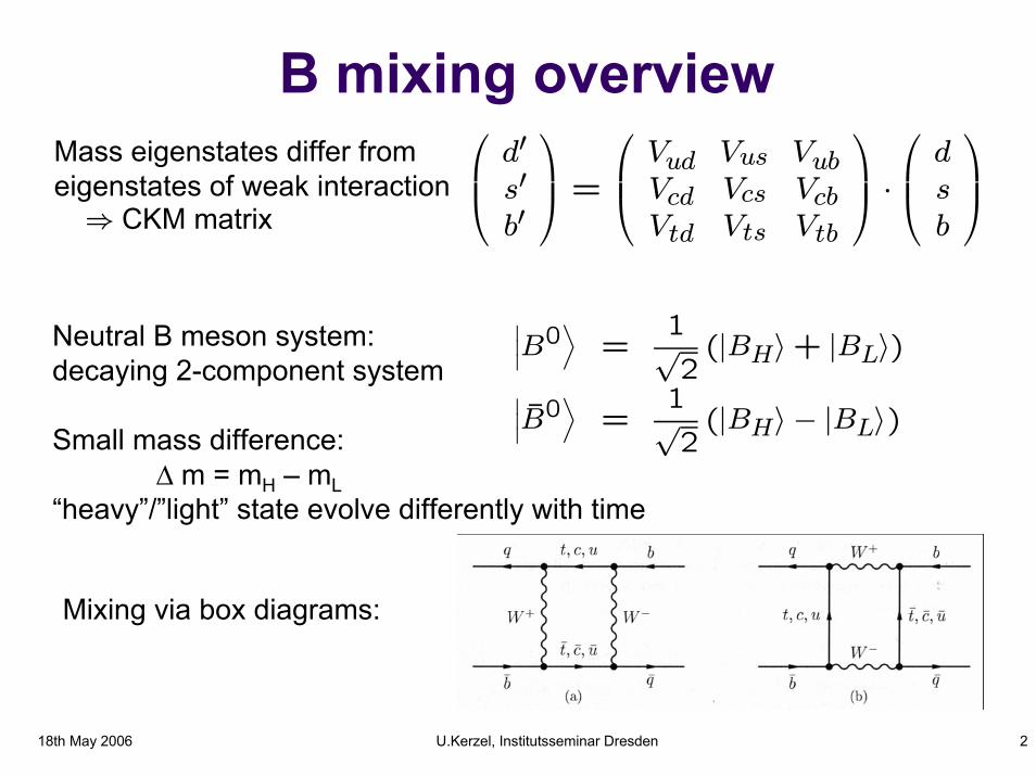
B mixing overview⎛⎜⎝ d0s0b0
⎞⎟⎠ =⎛⎜⎝ Vud Vus VubVcd Vcs VcbVtd Vts Vtb
⎞⎟⎠ ·⎛⎜⎝ dsb
⎞⎟⎠Mass eigenstates differ from eigenstates of weak interaction ⇒ CKM matrix
¯̄̄B0
E=
1√2(|BHi+ |BLi)¯̄̄
B̄0E=
1√2(|BHi− |BLi)
Neutral B meson system:decaying 2-component system
Small mass difference: Δ m = mH – mL
“heavy”/”light” state evolve differently with time
Mixing via box diagrams:

18th May 2006 U.Kerzel, Institutsseminar Dresden 3
B mixing overview
Δmq ∝ mBqB̂Bqf2Bq¯̄̄VtbV
∗tq
¯̄̄2From theory:
Uncertainties cancel in ratio: ΔmsΔmd
∝ |Vts|2|Vtd|2
w/o CDF Δ ms measurement
From CKM fit (EPS 2005):
Δms= 18.3+6.5−1.5 ps
−1
measure Δ ms:• determine ratio of CKM elements• probe for new physics

18th May 2006 U.Kerzel, Institutsseminar Dresden 4
B mixing overviewexperimentally accessible:
need to:• reconstruct Bs
(including decay vertex/lifetime)• tag flavour at production and decay
challenges:• momentum resolution• vertex resolution• tagging power
A(t) =Nmix(t)−Nunmix(t)Nmix(t)+Nunmix(t)
∝ cos(Δmqt)

18th May 2006 U.Kerzel, Institutsseminar Dresden 5
B mixing overviewFigure of merit: significance of mixing signal Moser, Roussarie (NIMA 384 491)
signi =
rS²D2
2 e−(Δmsσcτ )2
2
rS
S+B
S√S+B
optimise Bs candidate selection
σcτ optimise resolution
ε D2 optimise tagging performance² = NRS+NWS
N
D =NRS−NWSNRS+NWS
efficiency
dilution: Ameas = D Atrue

18th May 2006 U.Kerzel, Institutsseminar Dresden 6
Δ mq measurement: Amplitude method
assume fixed value of Δmq → fit for Amplituderepeat for different values of Δmq
e.g. B0 → D- π+
A(t) ∝ A × cos(Δ mq t)
A = 1 for correct Δ mqA = 0 else

18th May 2006 U.Kerzel, Institutsseminar Dresden 7
Δms from combined amplitude
combines:• LEP• CDF RunI• SLD

18th May 2006 U.Kerzel, Institutsseminar Dresden 8
CDF D0
Tevatron
Main injectorand recycler
RunI: 1992 – 1996data taking period at
RunII: 2001 – 2009major upgrades tocollider anddetectors
√s = 1.8TeV
The Tevatron
√s = 1.96 TeV
pp̄ collisions

18th May 2006 U.Kerzel, Institutsseminar Dresden 9
Tevatron performance
Running well - both peak luminosity and integrated luminositybefore shutdown: ~15-20 pb-1 / week delivered
1 fb-1 delivered in beginning of June 2005 .
1 fb-1

18th May 2006 U.Kerzel, Institutsseminar Dresden 10
CDF:• precise tracking:
silicon vertex detector and drift chamber• important for B physics:
direct trigger for displaced vertices
D0:• excellent muon system and coverage• large forward tracking coverage• new in RunII: magnetic field
⇒ D0 has joined the field of B physics

18th May 2006 U.Kerzel, Institutsseminar Dresden 11
Physics at the Tevatron• large b production rates:
⇒ 103 times bigger than !
• spectrum quickly falling with pt
• Heavy and excited states not produced at B factories:
• enormous inelastic cross-section:
⇒ triggers are essential
• events “polluted” by fragmentation tracks, underlying events
⇒ need precise tracking and good resolution!
Υ(4S)
Bc, Bs, B∗∗,Λb,Σb, . . .
σ(pp̄, |η| < 1.0) ≈ 20μb
`S
Belle engineering run

18th May 2006 U.Kerzel, Institutsseminar Dresden 12
Trigger in hadronic environment
• Dimuon: “easy” trigger, clean signal• sensitive to J/ ψ→ μ+ μ-
• low branching fraction
• Semi-leptonic B decays CDF: (μ, e) + displaced trackD0 : single (μ, e)
• Fully hadronic B decays (CDF)• BR ≈ 80%• require two displaced tracks• needs high precision tracking
at trigger level !
Primary Vertex
Secondary Vertex
d0 = impact parameter
B
Lxy
require:• pt > 2 GeV/c• 120 μm<|d0|<1mm
(not used for mixing analysis)
almost “offline” resolution

18th May 2006 U.Kerzel, Institutsseminar Dresden 13
Some sample events
recorded by J/ψ→ μ+ μ- trigger (CDF)
J/ ψ→ μ+ μ-
what all this fuzz about hadronic environment...

18th May 2006 U.Kerzel, Institutsseminar Dresden 14
Some sample events
recorded by J/ψ→ μ+ μ- trigger (CDF)
... well, usually events are like this...

18th May 2006 U.Kerzel, Institutsseminar Dresden 15
plot courtesy C. Lecci
B physics at low pt⇒ no “jet” structure
CDF RunII Simulation
Some sample events

18th May 2006 U.Kerzel, Institutsseminar Dresden 16
Hadronic vs. semi-leptonic B decays
hadronic decaysfully reconstructedhigh cτ resolutionlow candidate yield
semileptonic decayshigh yieldneutrino not reconstructed⇒ worse cτ resolution
Lxy =(~xdecay−~xprim)·~pt
|~pt|decay
PV
cτ = LxyM(B)
pt(B)
= LxyM(`D)
pt(`D)× K
hadronic
semi-leptonic
from simulation

18th May 2006 U.Kerzel, Institutsseminar Dresden 17
Bs reconstruction
Ds ≈ 26.7k events
D± ≈ 7.4k events
Exploit excellent muon coverage (single μ trigger):Bs → μ+Ds
-X, Ds- → φ π-, φ→ K+ K-

18th May 2006 U.Kerzel, Institutsseminar Dresden 18
Signal Yield Summary: Semi-leptonic
Bs → l Ds X Yield
Ds → (φπ) 32k
Ds → (K* K) 11k
Ds → (3π) 10k
Total 53k

18th May 2006 U.Kerzel, Institutsseminar Dresden 19
Signal Yield Summary: Hadronic
Yield
Bs→ Dsπ (φπ) 1600
Bs→ Dsπ (K* K) 800
Bs→ Ds π (3π) 600
Bs→ Ds3π (φ π) 500
Bs→ Ds3π (K*K) 200
Total 3700
oscill. fit range
partially reconstructed Bs

18th May 2006 U.Kerzel, Institutsseminar Dresden 20
Mixing measurement outline“same side”:(semi) exclusively reconstructed Bs
“opposite side”
1) decay flavour fromdecay products
2) proper time measurement
e, μoppositeside kaon
3) production flavour fromopposite side tag andsame-side Kaon tagger

18th May 2006 U.Kerzel, Institutsseminar Dresden 21
Flavour tagging methodssame side
oppositeside
opposite side: (CDF and D0)• jet charge
• (soft) lepton ID• flavour from semi-leptonic B decay (BR ≈ 20%)• dilution due to oscillation and cascade decays
(b → c → l X)
same side: (new at CDF)• same side Kaon tagging
kaon is (often) leading fragmentation partner of Bs⇒ particle ID is essential!
Qjet =Pi wiQiPi wi

18th May 2006 U.Kerzel, Institutsseminar Dresden 22
Flavour taggers at D0Deploy opposite side taggers:• lepton jet charge (in cone around lepton)
Ql = ∑i qi pti / ∑i pt
i
• secondary vertex jet chargeQSV = ∑i (qi pL
i)0.6 / ∑i (pLi)0.6
• event jet charge (outside cone around Bs)QEV = ∑i qi pt
i / ∑ pti
dtag=1−z1+z ; z = Πi
f b̄i (xi)
f bi (xi)combine via:
gives: ²D2 = 2.48± 0.21(stat)+0.08−0.06(syst)%

18th May 2006 U.Kerzel, Institutsseminar Dresden 23
Flavour taggers at CDF
Opposite side (OS) taggers: calibrated on l+SVT data• soft μ±, e±
• jet charge: with secondary vertex, with displaced tracks,other high pt jets
Same side (SS) tagger : calibrated in Bs → Ds π channel
most powerful tagger!• use one OS tag and SS tag to determine initial flavour,
• OS taggers mutually exclusive.
tagger ²D2[%]
combined OS 1.54± 0.04± 0.05SS Kaon 4.0+0.9−1.2

18th May 2006 U.Kerzel, Institutsseminar Dresden 24
Neural jet charge tagger
TrackNet:combines track quantities (e.g. pt,impact parameter, rapidity w.r.t., etc.)via NeuroBayes network⇒ probability to originate from B
B-Jet network:combines TrackNet + jet quantitiesvia NeuroBayes network⇒ identify B jets
⇒ significant improvementw.r.t. method based on impact parameter alone
note log-scale

18th May 2006 U.Kerzel, Institutsseminar Dresden 25
Same side kaon tagging
Kaon is (often) leading fragmentation partner• identified Kaon ⇒ identify Bs• charge of Kaon determines production flavour
⇒ very powerful tagger !
Challenges:• need good PID to identify Kaon: dE/dx + ToF (no RICH!)• has to be calibrated using simulation
→ difficult in hadronic environment

18th May 2006 U.Kerzel, Institutsseminar Dresden 26
Calibrating SSKTuse combined PID likelihood (ToF + dE/dx), select most “kaon-like” track in cone around B as tagging trackverify kinematic distributions (pT, tagging track pT, multiplicity, isolation) of light B mesons in Pythia simulationverify particle ID simulationtest for dependences on:
fragmentation modelbb production mechanismsdetector/PID resolutionmultiple interactionsPID content around B mesondata/MC agreement
test on high statistics lightB meson sample

18th May 2006 U.Kerzel, Institutsseminar Dresden 27
Δ ms measurement⇒ all ingredients there, determine Δ ms
• Amplitude method: scan Δ ms range, fit for asymmetry amplitude
• unbinned likelihood fit:
signal
combinatorial background
prompt background
“physics” background(other particle decays)
each part: contribution from mass, cτ, σ(cτ)
L = fsigLsig +fcombLcomb+fpromptLprompt+fphysLphys

18th May 2006 U.Kerzel, Institutsseminar Dresden 28
Bs mixing result
most probable value: Δ ms = 19 ps-1
17 < Δ ms < 21 ps-1 at 90% C.L.
resolution not sufficientto measure oscillationin this region
A/σA (19 ps-1) = 2.5
probability of bg fluctuation: (5.0 ± 0.3)%

18th May 2006 U.Kerzel, Institutsseminar Dresden 29
A/σA (17.25 ps-1) = 3.5
Bs mixing result
Δms = 17.33 +0.42 (stat) ± 0.07 (syst) ps-1-0.21
Δms in [17.00, 17.91] ps-1 at 90% CL Δms in [16.94, 17.97] ps-1 at 95% CL
Probability of bg fluctuation: 0.5%

18th May 2006 U.Kerzel, Institutsseminar Dresden 30
Systematic uncertainties on Δms
evaluated using toy MCsample compositionindividual event vertex uncertaintydilutiondetector resolution
Result is limited by statisticsdominant: lifetime measurement
Syst. Unc.
SVX Alignment 0.04 ps-1
Track Fit Bias 0.05 ps-1
PV bias from tagging 0.02 ps-1
All Other Sys < 0.01ps-1
Total 0.07 ps-1
All relevant systematic uncertainties are common between hadronic and semileptonic samples

18th May 2006 U.Kerzel, Institutsseminar Dresden 31
Impact on CKM fit
prior to new CDF result: with new CDF result:

18th May 2006 U.Kerzel, Institutsseminar Dresden 32
Impact on CKM fit
|Vtd||Vts| = 0.208
+0.08−0.07 (stat ⊕ syst)

18th May 2006 U.Kerzel, Institutsseminar Dresden 33
Further improvementsCDF:
Improved selection in hadronic modes using Neural NetworksUse partially reconstructed hadronic modesUse semileptonic events from other triggersImprove vertex resolution
D0:Addition of other taggersUse of other semileptonicdecay modesUse of hadronic decay modesImprove vertex resolution (inclusion of Layer0)

18th May 2006 U.Kerzel, Institutsseminar Dresden 34
Further improvementsdevelop inclusive B analysis package using NeuroBayes inspired by BSAURUS (DELPHI)
exploit all availableinformation vianeural networks

18th May 2006 U.Kerzel, Institutsseminar Dresden 35
NeuroBayes (1)Inspired by nature:Neuron in brain “fires” if stimuli received from other neurons exceed threshold. (very simple model. . . )
Construct Neural NetworkOutput of node j in layer n is given by weighted sum of output of all nodes in layer n-1:
xnj = g³P
k wnjk · xn−1k + μnj
´g(t) μnjsigmoid function threshold (“bias-node”)
→ information is stored in connections

18th May 2006 U.Kerzel, Institutsseminar Dresden 36
NeuroBayes (2)
Output
Input
Sign
ifica
nce
cont
rol
Postprocessing
Preprocessing
f t
Probability that hypothesisis correct
(classification)or probability densityfor variable t
t
Historic orsimulated data
Data seta = ...b = ...c = .......t = …!
NeuroBayesNeuroBayes®®TeacherTeacher
NeuroBayesNeuroBayes®®ExpertExpert
Actual (new real) data
Data seta = ...b = ...c = .......t = ?
ExpertiseExpertise
Expert system

18th May 2006 U.Kerzel, Institutsseminar Dresden 37
Classical ansatz:f(x|t)=f(t|x)
approximately correctat good resolution
far away fromphysical boundaries
Bayesian ansatz:takes into accounta priori- knowledge f(t):•Lifetime never negative•True lifetime exponentially
distributed
NeuroBayes (3)example: measured lifetime distribution

18th May 2006 U.Kerzel, Institutsseminar Dresden 38
Inclusive B analysisidentify B decay products and construct “best” B vertex

18th May 2006 U.Kerzel, Institutsseminar Dresden 39
Inclusive B analysisflavour tagging on track level:

18th May 2006 U.Kerzel, Institutsseminar Dresden 40
Inclusive B analysis(preliminary MC studies,for illustration only)

18th May 2006 U.Kerzel, Institutsseminar Dresden 41
Inclusive B analysisexploit all information
combined flavour tag

18th May 2006 U.Kerzel, Institutsseminar Dresden 42
Conclusions
Good performance of Tevatron and detectorsΔ ms (almost) measured
D0: two sided limit: 17 < Δ ms < 21 ps-1
A/σA ≈ 2.5 (for amplitude method) at 19 ps-1
Probability of background fluctuation: 5.0 ± 0.3 %
CDF: A/σA ≈ 3.5 (for amplitude method)Probability of background fluctuation: 0.5%
Aim for “5σ” discovery at summer conferencesextensive list of further improvements... no “new physics” here, it seems...
Δms= 17.33+0.42−0.21(stat)± 0.07(syst.)

18th May 2006 U.Kerzel, Institutsseminar Dresden 43
BACKUP

18th May 2006 U.Kerzel, Institutsseminar Dresden 44
• observe at• 1 fb-1 luminosity delivered early June• huge inelastic cross-section:≈ 5000 times bigger than for⇒ triggers are essential!
• events “polluted” by fragmentation tracks, underlying events⇒ need precise tracking and good resolution
pp̄ collision
Physics at the Tevatrons√s = 1.96 TeV
• dedicated trigger for J/Ψ→ μ+ μ-
• trigger events where m(μ+μ-) around m(J/Ψ)⇒ high quality J/Ψ events with large statistics
• channel J/Ψ→ e+e- much more challenging in hadronic environment
bb̄

18th May 2006 U.Kerzel, Institutsseminar Dresden 45
SVT based Triggers hadronic channelrequire two SVT tracks
pT>2GeV/cpT1+pT2 > 5.5 GeV/copposite charge 120 μm < SVT IP < 1 mmLxy > 200 μm
semileptonic channel require 1 Lepton + 1 SVT track
1 muon/electron pT> 4 GeV1 additional SVT track with
pT > 2 GeV120 μm < SVT IP < 1 mm
DP.V.
Lepton
Bν
SVT trackDP.V.
SVT track
B SVT track

18th May 2006 U.Kerzel, Institutsseminar Dresden 46
“Classic” B Lifetime Measurement
reconstruct B meson mass, pT, Lxycalculate proper decay time (ct)extract cτ from combined mass+lifetime fitsignal probability:psignal(t) = e-t’/τ⊗ R(t’,t)
● background pbkgd(t) modeled from sidebands
pp collision B decays
ct · pt/m

18th May 2006 U.Kerzel, Institutsseminar Dresden 47
Hadronic Lifetime Measurement
SVT trigger, event selection sculpts lifetime distributioncorrect for on average using efficiency function:
p = e-t’/τ⊗ R(t’,t) ·ε(t)efficiency function shape contributions:
event selection, triggerdetails of efficiency curve
important for lifetime measurementinconsequential for mixing measurement
pattern limit|d0| < 1 mm
“trigger” turnon
0.0 0.2 0.4proper time (cm)

18th May 2006 U.Kerzel, Institutsseminar Dresden 48
Hadronic Lifetime Results
ModeLifetime [ps](stat. only)
B0 → D- π+ 1.508 ± 0.017
1.638 ± 0.017
1.538 ± 0.040
B- → D0 π-
Bs → Ds π(ππ)
World Average:
B0 → 1.534 ± 0.013 ps-1
B+ → 1.653 ± 0.014 ps-1
Bs → 1.469 ± 0.059 ps-1
Excellent agreement!

18th May 2006 U.Kerzel, Institutsseminar Dresden 49
Semileptonic Lifetime Measurement
neutrino momentum not reconstructed
correct for neutrino on average

18th May 2006 U.Kerzel, Institutsseminar Dresden 50
lDs ct* Projections
Bs lifetime in 355 pb-1: 1.48 ± 0.03 (stat) psWorld Average value: 1.469 ± 0.059 ps
Lepton
Ds- vertex
P.V.Bs vertex

18th May 2006 U.Kerzel, Institutsseminar Dresden 51
Unbinned Likelihood Δmd Fits
hadronic: Δmd = 0.536 ± 0.028 (stat) ± 0.006 (syst) ps-1
semileptonic: Δmd = 0.509 ± 0.010 (stat) ± 0.016 (syst) ps-1
world average: Δmd = 0.507 ± 0.005 ps-1
fit separately in hadronic and semileptonic sampleper sample, simultaneouslymeasure
tagger performanceΔmd
projection incorporatesseveral classes of tags
semileptonic, lD-, muon tag

18th May 2006 U.Kerzel, Institutsseminar Dresden 52
Systematic uncertaintiesSilicon detector alignment
Effect of imperfect alignment of silicon vertex detector on lifetime measurement. Tested by introducing distortions into realistic simulation measuring lifetime with default alignment
Track-fit biasMis-measurement of pt introduces mis-measurement of Lxy and lifetime. Tested with realistic simulation.
Primary vertex biasMis-measurement of primary vertex leads to mis-measurement of Lxyand lifetime, cause a bias when tracks from opposite side are incorporated into primary vertex. Studied with large sample of fully reconstructed B events comparing reconstructed primary vertex with average beam position

18th May 2006 U.Kerzel, Institutsseminar Dresden 53
Conditional probability densities f(t|x)
Conditional probability densities f(t|x) are functions of x, but also depend on marginal distribution f(t).
Conditional probability densities f(t|x) are functions of x, but also depend on marginal distribution f(t).
Conditional probability density for a special case x
(Bayesian Posterior)
Conditional probability density for a special case x
(Bayesian Posterior)
Inclusive distribution(Bayesian Prior)
Inclusive distribution(Bayesian Prior)
Marginal distribution f(t)Marginal distribution f(t)
Bayesian approach

18th May 2006 U.Kerzel, Institutsseminar Dresden 54