bubble velocity, size and interfacial area measurements in bubble columns

WASHINGTON UNIVERSITY

SEVER INSTITUTE OF TECHNOLOGY

DEPARTMENT OF CHEMICAL ENGINEERING

BUBBLE VELOCITY, SIZE AND INTERFACIAL AREA

MEASUREMENTS IN BUBBLE COLUMNS

By

Junli Xue

Prepared under the direction of

Prof. M. P. Duduković, Prof. M. H. Al-Dahhan & Prof. R. F. Mudde

Thesis presented to the Sever Institute of Washington University

in partial fulfillment of the requirements of the degree of

DOCTOR OF SCIENCE

December 2004

Saint Louis, Missouri

WASHINGTON UNIVERSITY

SEVER INSTITUTE OF TECHNOLOGY

DEPARTMENT OF CHEMICAL ENGINEERING

ABSTRACT

BUBBLE VELOCITY, SIZE AND INTERFACIAL AREA MEASUREMENTS IN

BUBBLE COLUMNS

By Junli Xue

ADVISOR: Professor M. P. Duduković, Professor M. H. Al-Dahhan and

Professor R. F. Mudde

December 2004

Saint Louis, Missouri

The knowledge of bubble properties, including bubble velocity, bubble size, gas holdup,

and specific interfacial area, is of importance for the proper design and operation of

bubble columns. A four-point optical probe was adopted in this study to measure bubble

properties in such systems. An improved algorithm for data processing was developed,

which extends the capability of the probe and improves the accuracy of the measurement.

The new algorithm provides both the magnitude and direction angles of the bubble

velocity vector. The results from the probe and the algorithm were validated against

video imaging and it was established that the bubble velocity distribution, bubble chord

length distribution, local gas holdup, and specific interfacial area obtained by the four-

point optical probe are reliable.

The four-point optical probe measurements of bubble properties were taken in an air-

water system using a 16.2cm (6.4”) diameter bubble column at elevated pressure, up to

1.0 MPa, and at high superficial gas velocity, up to 60 cm/s, equipped with three different

gas spargers.

It was established that gas holdup radial profiles evolve from flat at low superficial gas

velocity to highly parabolic at high superficial gas velocity. Specific interfacial area

profiles, bubble mean velocity profiles, and bubble frequency profiles exhibit the same

trends. Bubble velocity distributions change from unimodal to bimodal with increase in

superficial gas velocity. However, only unimodal bubble size distributions were

observed. The effects of pressure, spargers, and elevation in the column are also

illustrated.

This study establishes the four-point probe as a useful tool for study of bubble properties

in actual bubble columns.

iii

Contents

List of Tables ................................................................................................................ v

List of Figures............................................................................................................... vi

Acknowledgements ...................................................................................................... xii

Nomenclature ............................................................................................................... xiv

1. Introduction............................................................................................................. 1

1.1 Motivation....................................................................................................... 1

1.2 Research Objectives........................................................................................ 4

2. Background ............................................................................................................. 6

2.1 Bubbles’ Behavior in (Slurry) Bubble Columns............................................. 6

2.1.1 Bubble Shape, Motion, and Size Distribution ................................... 6

2.1.2 Gas Liquid Flow Patterns and Flow Regimes (Hydrodynamics) ...... 11

2.1.3 Effect of Operating Conditions on Hydrodynamics .......................... 14

2.1.4 Specific Interfacial Area .................................................................... 16

2.2 Type of Probes Used in Multiphase Systems ................................................. 25

3. Suggested Algorithm for the Four-Point Optical Probe ..................................... 38

3.1 Analysis of Measurement Errors of Two-Point Probes .................................. 38

3.2 The Configuration and Principle of the Four-Point Optical Probe................. 44

3.2.1 The Configuration of the Four-Point Optical Probe ........................... 44

3.2.2 Working Principle of the Four-Point Optical Probe ........................... 48

3.2.3 Signal Analysis ................................................................................... 51

3.2.4 Measurement Errors of the Four-Point Optical Probe (Old Algorithm)

............................................................................................................. 56

3.3 New Data Processing Algorithm for the Four-Point Probe ............................ 68

4. Validation of Measurements by the Four-Point Optical Probe.......................... 79

4.1 Validation of the Bubble Velocity Vector ...................................................... 79

4.2 Validation of the Specific Interfacial Area ..................................................... 96

iv

4.3 Validation of the Local Gas Holdup ............................................................... 100

5. Bubble Properties in Bubble Columns Obtained by the Four-Point Optical

Probe .................................................................................................................... 110

5.1 Experimental Setup......................................................................................... 110

5.2 Comparison of the Gas Holdup Profile Obtained by Probe and by CT.......... 113

5.3 The Effect of Superficial Gas Velocity........................................................... 117

5.4 The Effect of Pressure..................................................................................... 129

5.5 The Effect of Spargers .................................................................................... 135

5.6 The Effect of Axial Position ........................................................................... 140

5.7 The Sauter Mean Bubble Diameter ................................................................ 147

5.8 The Bubble Size Distribution ......................................................................... 149

5.9 The Mean Gas-Liquid Slip Velocity............................................................... 156

6. Conclusions and Future Works ............................................................................. 159

Appendix A. The Plastic Fiber Optical Probe........................................................... 163

Appendix B. Derivation of the Transformation Matrix ........................................... 165

Appendix C. The Natural Frequency of the Optical Probe ..................................... 166

Appendix D. Additional Bubble Properties in Bubble Columns Obtained by the

Four-Point Optical Probe ..................................................................... 167

D.1 Comparison of the Gas Holdup Profile Obtained by Probe and by CT......... 167

D.2 The Effect of Superficial Gas Velocity.......................................................... 172

D.3 The Effect of Pressure.................................................................................... 176

D.4 Transformation from Bubble Size Distribution to Bubble Chord Length

Distribution.................................................................................................... 176

D.5 Summary ........................................................................................................ 180

Appendix E. Testing of Phase Transition At Subcritical and Supercritical

Conditions Using Four-Point Optical Probe....................................... 181

Appendix F. Derivation of The Bubble Size and Aspect Ratio................................ 183

References ..................................................................................................................... 185

Vita ................................................................................................................................ 195

v

Tables

2-1. Existing Data Sets for Specific Interfacial Area Taken in Bubble Columns

(Hibiki and Ishii, 2002)...................................................................................... 22

4-1. Statistical Parameters for the Bubble Velocity Distributions ............................ 89

4-2. Statistical Parameters for the Bubble Direction Angle Distributions................ 91

4-3. Comparison of Specific Interfacial Areas.......................................................... 100

4-4. Local Gas Holdup Obtained by the Probe and by the Camera .......................... 105

5-1. Column Dimensions and Selected Operating Conditions.................................. 112

5-2. Sparger Configurations ...................................................................................... 112

5-3. Comparison of the Integrated Cross-Sectional Gas Holdup and the Overall

Gas Holdup at High Pressures (Sparger #3, Ug=30 cm/s) ................................ 116

5-4. Comparison of the Predicted Initial Bubble Size and Mean Bubble Chord

Length Obtained by the Four-Point Optical Probe ............................................ 137

D-1. Comparison of the Local Gas Holdup Obtained by CT and by Probe............... 169

D-2. Comparison of the Local Gas Holdup Obtained by CT and by Probe

(Sparger#3, Ug=30 cm/s, z/D=5.1).................................................................... 170

D-3. Comparison of the Integrated Cross-Sectional Gas Holdup and the Overall

Gas Holdup ........................................................................................................ 171

D-4. Statistical Parameters of the Bubble Velocity Distribution............................... 175

D-5. Pressure Effect on the Mean and Standard Deviation of the Bubble Velocity

Distribution ........................................................................................................ 176

D-6. Change of Bubble Properties with Operating Conditions ................................. 180

vi

Figures

2-1. Sketches of Various Bubble Shapes Observed in Infinite Newtonian Liquid

(Bhaga and Weber, 1981) .................................................................................. 7

2-2. Flow Regimes in a 3-D Bubble Column (Chen, Reese and Fan, 1994) ............ 11

2-3. Flow Structure in the Vortical-spiral Flow Regime in a 3-D Gas-Liquid

Bubble Column (Chen, Reese and Fan, 1994)................................................... 12

2-4. Various Tip Configuration of Two-point Probes (Choi and Lee, 1990) ........... 26

2-5. Schematic Diagram of a Double-Sensor Conductivity Probe (Wu and Ishii,

1999) .................................................................................................................. 27

2-6. Schematic Diagram of a Five-Sensor Conductivity Probe (Burgess and

Calderbank, 1975).............................................................................................. 28

2-7. Schematic of the Multineedle Conductivity Probe and the Bubble Shape

Detected (Iguchi, Nakatani and Kawabata, 1997) ............................................. 29

2-8. A Light Transmittance Probe (Kuncova, Zahradnik and Mach, 1993) ............. 30

2-9. A Light Transmittance Probe (Kreischer, Moritomi and Fan, 1990) ................ 31

2-10. A Reflective Fiber Optic Sensor (Farag et al., 1997) ........................................ 32

2-11. Schematic of the Snell’s Law (Abuaf et al., 1978)............................................ 33

2-12. The Effect of a Thin Liquid Film on the Probe Tip (Frijlink, 1987) ................. 34

2-13. Schematic Representation of an Optical Probe (Abuaf et al., 1978)................. 35

2-14. A U-Shape Light Reflective Probe (Yu and Kim, 1988)................................... 35

2-15. A Spherical Bulb Dual Optical Fiber Probe (Chabot et al., 1992) .................... 36

2-16. Examples of the Probe Tips Produced by Etching Optical Fibers (O.D. 140

µm) (Cartellier, 1998) ........................................................................................ 37

3-1. Schematic of the Bubble Behavior Measurement by a Two-Point Probe ......... 40

3-2. Curvature Correction ......................................................................................... 41

3-3. Relative Error in (a) the Bubble’s Vertical Velocity and (b) the Bubble Chord

Length Obtained by a Two-Point Probe ............................................................ 44

3-4. Configuration of the Four-Point Optical Probe ................................................. 46

vii

3-5. Jig for the Fabrication of the Four-point Probe ................................................. 47

3-6. The Four-point Optical Probe Installed in a 2D Bubble Column...................... 48

3-7. The Schematic of the Light Splitter ................................................................... 49

3-8. Response of the Four-Point Probe to a Bubble Pierced Through ...................... 50

3-9. Schematic of the Response of the Four-Point Probe to a Bubble Pierced

Through.............................................................................................................. 51

3-10. A Sample of the Probe’s Responses .................................................................. 53

3-11. Relationship between Gas Holdup and the Threshold Selected ........................ 54

3-12. Schematic of the Selection Function of the Four-point Probe........................... 55

3-13. Schematic of the Probe Tips and Bubble Velocity Vector ................................ 57

3-14. Coordinate Transformation................................................................................ 58

3-15. Relative Errors in Bubble Velocity Measurements due to the Deviation of

Bubble motion from the Probe’s Axial Direction (r=0.6mm, L=1.5mm) ......... 61

3-16. The Tolerance for Tip1 When Bubbles Deviated from the Probe’s Axial

Direction ............................................................................................................ 62


Direction ............................................................................................................ 63


Direction ............................................................................................................ 64

3-19. Bubbles in a 2D Bubble Column (181.5×49.0×1.3 cm) at Superficial Gas

Velocity Ug=1.85 cm/s ...................................................................................... 65

3-20. Bubble Chord Length Measured by the Probe................................................... 67

3-21. Schematic of the Principle of the New Data Processing Algorithm.................. 69

3-22. Determination of the Bubble Size and Aspect Ratio ......................................... 72

3-23. The Physical Situation of the Bubble Velocity Measurements ......................... 74

3-24. The Physical Situation of the Measurements of the Specific Interfacial Area

by the Four-Point Probe..................................................................................... 76

4-1. The Calibration Setup ........................................................................................ 80

4-2. Bubble Hits the Probe Tip (field of view 1.3cm×1.3cm) .................................. 81

4-3. Influence of Probe and Bubble Interaction on Bubble Velocity........................ 81

viii

4-4. Comparison of Bubble Velocity and Bubble Chord Length, Error = (value by

probe- value by camera)/ value by camera × 100%........................................... 82

4-5. Setup of the 2D Bubble Column for the Probe Validation ................................ 84

4-6. Rotation of Bubbles in the 2D Bubble Column................................................. 85

4-7. Comparison of Bubble Velocity Distributions Obtained by the Four-Point

Optical Probe and by Video Imaging ................................................................ 88

4-8. Comparison of Bubble Direction Angle Distributions ...................................... 91

4-9. Projection of the Velocity Vector on Camera Photos........................................ 92

4-10. Setup for the Validation of Bubble Velocity ..................................................... 93

4-11. Relative Errors in the Mean Bubble Velocity vs. (a) Bubble Reynold Number

and (b) Bubble Eotvos Number (Morton Number = 2.65×10-11) ...................... 95

4-12. Relative Error in the specific Interfacial Area Obtained by Equation (4.3) ...... 98

4-13. Setup for the Validation of Local Gas Holdup .................................................. 101

4-14. Measurement of Gas Holdup by the Optical Probe ........................................... 102

4-15. Comparison of Local Gas Holdup Obtained by Probe and by Camera ............. 105

4-16. Distribution of the Time Intervals that the Probe’s Central Tip Spends in

Bubbles .............................................................................................................. 106

4-17. Deformation of the Bubble’s Leading Edge due to the Interaction with the

Probe Tip............................................................................................................ 107

5-1. The Configuration of the Bubble Column ......................................................... 111

5-2. Sparger Configurations ...................................................................................... 112

5-3 Comparison of Gas Holdup by CT and by Probe at Atmospheric Pressure

(Sparger #2) ....................................................................................................... 115

5-4. Comparison of Radial Profiles of Gas Holdup by CT and Probe at High

Pressures (Sparger #3, 30 cm/s, z/D=5.1).......................................................... 116

5-5. The Radial Profile of Local Gas Holdup and Specific Interfacial Area

(Sparger #2, z/D=5.1) ........................................................................................ 118

5-6. The Radial Profile of Mean Bubble Velocity and Its Change with Ug

(Sparger #2, z/D=5.1) ........................................................................................ 120

ix

5-7. Bubble Velocity Distribution in the Wall Region at Different Superficial Gas

Velocities (z/D=5.1, Sparger #2) ........................................................................ 123

5-8. Bubble Velocity Distribution at Different Superficial Gas Velocities (r/R=0,

z/D=5.1, Sparger #2).......................................................................................... 124

5-9. Bubble Chord Length Distribution at Different Superficial Gas Velocities

(Sparger #2, 0.1MPa, z/D=5.1).......................................................................... 125

5-10. The (a) Mean and (b) Standard Deviation of the Bubble Chord Length

Distribution at Different Superficial Gas Velocities.......................................... 126

5-11. Bubble Velocity and Bubble Chord Length Distribution at Different Radial

Positions (Sparger #2, Ug=60 cm/s, z/D=5.1) ................................................... 127

5-12. Bubble Velocity vs. Bubble Chord Length........................................................ 129

5-13. Pressure Effect on (a) Gas Holdup and (b) Specific Interfacial Area (Sparger

#3, 30 cm/s, z/D = 5.1)....................................................................................... 130

5-14. Pressure Effect on Bubble Frequency (Sparger #3, 30 cm/s) ............................ 131

5-15. Pressure Effect on Mean Bubble Velocity (Sparger #3, 30 cm/s, z/D = 5.1) .... 132

5-16. Pressure Effect on Bubble Velocity Distribution (Sparger #3, 30 cm/s, z/D =

5.1) ..................................................................................................................... 133

5-17. Pressure Effect on the Bubble Chord Length Distribution and Mean Bubble

Chord Length (Sparger #3, 30 cm/s) ................................................................. 134

5-18. Sparger Effect on Bubble Frequency in the Sparger Zone (z/D=1.7,

Ug=30cm/s, 0.1 MPa) ........................................................................................ 135

5-19. Sparger Effect on Bubble Chord Length Distribution and Local Gas Holdup

(0.1MPa, 30 cm/s, z/D = 1.7, r/R=0) ................................................................. 136

5-20. Sparger Effect on Bubble Velocity Distribution and Local Gas Holdup

(0.1MPa, 30 cm/s, z/D = 1.7)............................................................................. 138

5-21. Sparger Effect on Specific Interfacial Area (0.1MPa, 30 cm/s, z/D = 1.7) ....... 139

5-22. Bubble Properties at z/D=5.1 for Different Spargers ........................................ 140

5-23. Gas Holdup Profile at Different Axial Positions at High Pressure (Sparger

#3, Ug=30 cm/s) ................................................................................................ 142

5-24. Large Bubble and Small Bubble Holdups (r/R=0) ............................................ 143

x

5-25. Bubble Frequency Profile at Different Axial Positions (Sparger #3,

Ug=30cm/s) ....................................................................................................... 144

5-26. Bubble Chord Length Distributions at High Pressure (r/R=0) .......................... 145

5-27. Specific Interfacial Area Profile at High Pressure............................................. 146

5-28. Mean Bubble Velocity Profile at Different Axial Positions (Sparger #2,

0.1MPa).............................................................................................................. 147

5-29. Sauter Mean Bubble Diameter at Different Ug (Sparger #2, 0.1 MPa,

z/D=5.1) ............................................................................................................. 148

5-30. Sauter Mean Bubble Diameter at Different Pressures (Sparger #3,

Ug=30cm/s, z/D=1.7) ........................................................................................ 149

5-31. Gas Holdup Model in Bubble Columns Proposed by Krishna, Wilkinson, and

van Dierendonck (1991) .................................................................................... 150

5-32. Time Based Bubble Chord Length Distribution Obtained by the Probe ........... 151

5-33. Local Gas Holdup Obtained by the Probe ......................................................... 152

5-34. Time Based Bubble Chord Length Distribution ................................................ 153

5-35. Effect of Pressure on Time Based Bubble Chord Length Distribution and Gas

Holdups (Sparger #3, Ug=30 cm/s, r/R=0, z/D=5.1)......................................... 154

5-36. Volume Based Bubble Chord Length Distribution............................................ 153

5-37. Bubble Slip Velocity at Different Conditions.................................................... 158

A-1. The Tip Shape and the Response of a Single Plastic Optical Fiber to a Bubble

Passage............................................................................................................... 164

D-1. Comparison of Radial Profiles of Gas Holdup by CT and by Probe ................. 167

D-2. The Radial Profile of Bubble Frequency (Sparger #2, z/D=5.1) ....................... 173

D-3. Comparison of the Bubble Velocity Distribution Obtained by Two-Point

Probe and Four-Point Probe (r/R=0, z/D=5.1, Sparger #2) ............................... 174

D-4. Volume Based Bubble Chord Lengths Distribution Obtained by Four-Point

Optical Probe (r/R=0, z/D=5.1) ......................................................................... 177

D-5. The Bubble Size and Chord Length Distribution Calculated ............................ 179

E-1. Setup for the Detection of Phase Transition at Subcritical and Supercritical

Conditions .......................................................................................................... 182

xi

F-1. Comparison of Bubble’s Aspect Ratio and the Length of Major Axis

Obtained by Camera and by Four-Point Optical Probe (mean bubble velocity

32.2 cm/s, mean bubble size 0.23cm) ................................................................ 184

xii

Acknowledgements

The accomplishments presented in this thesis would not have been possible without the

support of many people. I wish to express my deepest gratitude to my advisors Prof. M.

P. Dudukovic, Prof. M. H. Al-Dahhan and Prof. R. F. Mudde for their guidance,

encouragement and constructive criticism. I would like to thank the members of my

committee, Prof. P. A. Ramachandran, Prof. R. A. Gardner, Prof. Sureshkumar and Dr. B.

A. Toseland of Air Products and Chemicals, Inc. for investing their valuable time in

examining my thesis and providing me with useful comments. Especially Dr. B. A.

Toseland for the numerous discussions and comments that helped me to better focus on

the real goals of my research in keeping it relevant to industrial practice.

I would like to acknowledge partial support from DOE Contract FC 2295 PC 95051 via

Air Products and Chemicals Inc. and CREL industrial sponsors, which financially made

this work possible.

I want to thank the members of CREL for their help. My special thanks goes to Dr. P.

Chen and Dr. Rafiq for sharing their knowledge with me and their valuable discussions

and suggestions.

During the course of my study numerous devices and pieces of equipment needed to be

designed and machined. I am very thankful to Mr. Pat Harkins and Jim Linders for their

fine work in machining of these devices. I am also thankful to Steve Picker whose large

experience helped me in solving various technical issues effectively.

Furthermore, I would like to thank Professor James Ballard of the Technical Writing

Center for helping me to improve the language in my thesis.

xiii

I wish to thank the secretaries of the Department of Chemical Engineering for their

prompt help in numerous administrative issues. I wish to thank to faculty, associates and

students of the Department of Chemical Engineering for making my overall graduate

school experience enjoyable.

And last but not least, my deepest gratitude is to the each and every member of my

family for their absolute support. Especially, I am grateful to my wife Yingjian Zhao and

my son Jiarui Xue for sharing all ups and downs, for their support and most of all, for

their understanding.

Nomenclature

a gas-liquid specific interfacial area, m2/m3

b the length of minor axis of an ellipsoidal bubble, cm

c the length of major axis of an ellipsoidal bubble, cm

D column diameter, cm

ds Sauter mean bubble diameter, mm

de volume equivalent bubble diameter, mm

DH the hydraulic equivalent diameter of the flow channel, cm

Eob bubble Eotvos number

g acceleration of gravity, m/s2

Li the bubble chord length pierced by the ith tip of the probe, cm

Mo Morton number

n bubble’s normal vector

HI the initial liquid phase height, cm

HD dynamic height of the gas-liquid system, cm

L the axial distance between peripheral tips and the central tip of the probe, cm

r the radial distance between peripheral tips and the central tip, mm

Reb Bubble Reynolds number

r/R radial position in the bubble column

∆T measurement time, s

∆ti time intervals between a bubble hitting the central tip T0 and it hitting tip Ti, s

Ti the time interval during which the ith, i=0,1,2,3, tip of the probe is inside the

bubble, s

th bubble discarding threshold

v the bubble velocity, cm/s

V the total volume of the gas-liquid mixed phase, m3

xiv

xv

Web bubble Weber number

z axial position, cm

Greek Letters

α aspect ratio of the ellipsoidal bubble, α=(length of vertical axis)/(length of

horizontal axis)

δv bubble selection tolerance

εg gas holdup

ϕ the angle of the projection of the bubble velocity vector on the xy plane to the x

axis, degree

θ the angle between the bubble velocity vector and the probe’s axial direction,

degree

φ the angle between the velocity vector and the normal vector of the gas-liquid

interface, degree

ρ density, Kg/m3

σ surface tension, N/m

µ viscosity, mPa⋅s

ν kinematic viscosity, m2/s

Subscripts

g gas phase

l liquid phase

T time based

V volume based

1

Chapter 1 Introduction

1.1 Motivation

Bubble column reactors are used extensively to perform a wide variety of gas/liquid or

gas/liquid/solid reactions, such as oxidation, hydrogenation, chlorination, aerobic

fermentation, waste water treatment, and coal liquefaction (De Swart and Krishna, 1995;

Jager and Espinoza, 1995; Shollenberger et al., 1997; Eisenberg et al., 1994; Davis,

2002). The main advantages of bubble columns over other multiphase reactors (stirred

vessels, packed towers, trickle bed reactors etc.) include simple construction, low

maintenance due to the absence of moving parts, excellent heat transfer properties, easy

temperature control, and reasonable interphase mass transfer rates at low energy input.

The knowledge of bubble properties, including bubble velocity, bubble size, gas holdup,

and specific interfacial area, is of considerable importance for the proper design and

operation of bubble columns. For example, the overall mass transfer rate per unit volume

of the dispersion in a bubble column is governed by the liquid-side volumetric mass

transfer coefficient (kla), assuming that the gas-side resistance is negligible. In a bubble

column reactor, the variation in kla is primarily due to variations in the specific interfacial

area, a. The specific gas-liquid interfacial area, a, is related to the gas holdup, εg, and the

bubble size distribution, while the gas holdup is determined by the bubble size

distribution, bubble velocity (i.e., bubble residence time), and bubble frequency. In the

same way, bubble properties play key roles in determining the heat transfer rate in bubble

columns (Yang et al., 2000). Furthermore, bubble size distribution and bubble velocity

distribution are key parameters in evaluating the drag forces on bubbles and in using the

bubble population balance in Computational Fluid Dynamics (CFD).

2However, the measurement of bubble size, bubble velocity, and specific interfacial area

in two and three-phase systems has always been a challenging problem. The problem is

even much more complex when the system being considered is no longer in the bubbly

flow regime, but rather in the chaotic churn-turbulent flow regime and at high pressure,

conditions which are of industrial interest.

The appeal of non-invasive techniques has led to attempts to capture the bubble size

distribution bubble velocity distribution by video imaging techniques (Patel, Daly and

Buckar, 1990; Idogawa, 1997; Luewisutthichat, Tsutsumi and Yoshida, 1997a; Mihai and

Pincovschi, 1998; Marques et al., 1999). However, video imaging can be used only in 2-

D transparent columns at low gas holdup, where light can penetrate the system. In real 3-

D columns, even with transparent walls, this technique provides no hope of capturing

anything beyond the reactor wall. Video imaging also cannot be used in systems where

the columns are operated at high temperature and high pressure and thus cannot be made

of transparent materials. Thus, invasive techniques are still the state of the art when it

comes to bubble size and bubble velocity measurements in practical 3-D multiphase

systems.

In recent years, optical and conductivity microprobes have been most frequently

employed to investigate bubble properties (Vince et al., 1982; Matsuura and Fan, 1984;

Lee, De Lasa and Bergougnou, 1986; Saxena, Rao and Saxena, 1990; Chabot et al., 1992;

Kuncova, Zahradnik and Mach, 1993; Groen et al., 1996; Farag et al., 1997; Luo et al.,

1998; A. Cartellier, 1998; Mudde and Saito, 2001). Conductivity probes utilize the

difference in electrical conductivity between the liquid phase and the gas phase. Optical

fiber probes make use of the difference in the refractive index between the gas phase and

the liquid phase and provide a sequence of voltage pulses when a bubble passes by the

probe. In comparison with conductivity probes, optical probes offer significant

advantages: 1) They can be used in conductive as well as non-conductive (organic)

systems, which are important in the petrochemical industry. 2) The presence of a liquid

film on the sensor tip reduces the effectiveness of a conductivity probe but not that of an

3optical probe. Therefore the sensitivity of optical probes is higher than that of

conductivity probes (van der Lans, 1985). 3) Optical probes achieve a much better

signal/noise ratio than conductivity probes.

At present, optical probes have been used mainly to determine bubble size and velocity

for individual bubbles in bubbly flows of modest gas holdup. There is no firm

experimental data or theory that can guide us as to how to use these probes and interpret

their signals in churn-turbulent flow with significant bubble coalescence and re-

dispersion and with a wide distribution of bubble sizes. The goal of this work is to

explore what bubble phase information can be obtained in churn-turbulent flows using

optical probe and make necessary modifications to the data processing algorithm.

For many years now, Washington University’s Chemical Reaction Engineering

Laboratory (CREL) has used Computer Tomography (CT) and Computer Automated

Radioactive Particle Tracking (CARPT) to investigate the gas holdup distribution and the

liquid phase recirculation in bubble columns. The gas holdup obtained by the optical

probe in the current study can be compared with values already obtained by CT for

validation. Moreover, gas holdup is qualitatively determined by the bubble velocity and

the bubble size distribution. Hence, by investigating these bubble properties, the

mechanism for changes in the gas holdup profiles with changing operating conditions can

be disclosed. Furthermore, in bubble columns the liquid recirculation derives from and

interacts with bubble properties. Hence, the combination of the measurement results from

CARPT with bubble properties obtained by the probe can give a clearer understanding of

the hydrodynamics in bubble columns.

In CFD, the population balance model, applied to gas bubbles, is needed to provide a

statistical formulation to describe the gas phase in bubble columns. The bubble size and

velocity distribution functions are employed in the population balance model. So far,

either a ‘mean’ bubble size is assumed or the bubble size distribution is predicted from

the bubble breakup and coalescence model. This can be much improved by comparing

4the experimental results for the bubble velocity and size distribution obtained by the

probe with the predictions generated by the model. Furthermore, two-fluid model based

codes (e.g., FLUENT, CFX, CFDLIB) cannot predict well the observed gas holdup radial

profiles, even in 3D simulations. With the bubble velocity and size distribution obtained

by the probe, the prediction of the gas holdup profile in CFD can be improved, which

would substantially increase the capability of CFD modeling of bubble column reactors.

This improvement, however, is beyond the scope of this thesis.

1.2 Research Objectives

The overall objective of this work is to investigate the bubble velocity distribution,

bubble chord length distribution, local gas holdup, and specific interfacial area as a

function of operating conditions (i.e., superficial gas velocity, pressure etc.) in both

bubbly flow and in churn-turbulent flow in bubble columns. Four major research goals

are:

(1) Modify the data processing algorithm to improve the capability of the four-point

optical probe to set up a practical tool for investigating bubble properties in bubble

columns in both bubbly flow and churn-turbulent flow.

(2) Validate the four-point optical probe and the developed novel data processing

algorithm versus video imaging in validation setups, e.g., a 2-D bubble column, at

different conditions.

(3) Use this probe in a 6.4” bubble columns to study the bubble velocity distribution,

bubble chord length distribution, gas holdup, and the specific interfacial area at

superficial gas velocity up to 60 cm/s, pressure up to 1.0 MPa, and for different spargers.

These operating conditions are the same as those at which the CT and CARPT

experiments were carried out in CREL (Bong Cheng Ong, 2003). These data are

nonexistent in the literature.

5

(4) Obtain deeper understanding of the hydrodynamics of bubble columns by analyzing

such data.

6

Chapter 2 Background

2.1 Bubbles’ Behavior in (Slurry) Bubble Columns

The research presented in the literature has captured some aspects of the behavior of

bubbles in bubble columns and slurry bubble columns. The following are the results

pertinent to this study.

2.1.1 Bubble Shape, Motion, and Size Distribution

Bubbles in motion are generally classified by shape as spherical, oblate ellipsoidal, and

spherical/ellipsoidal cap, etc. (Figure 2-1). The actual bubble shape depends on the

relative magnitudes of the forces acting on the bubble, such as surface tension and inertial

forces (Bhaga and Weber, 1981). When the bubble size is small (for example, volume

equivalent bubble diameter de<1mm in water), the surface tension force predominates

and the bubble is approximately spherical.

For bubbles of intermediate size, the effects of both surface tension and the inertia of the

medium flowing around the bubble are important. As a result, intermediate-size bubbles

exhibit very complex shapes and motion characteristics. While called ellipsoidal bubbles,

they often lack fore-and-aft symmetry and, in extreme circumstances, cannot be

described by any simple regular geometry, due to significant shape fluctuations (Bhaga

and Weber, 1981). This complex shape results from the superposition of various modes

of fluctuations that are of different amplitudes and take place at different frequencies

(Hibino, 1969). The dominant mode of shape fluctuations has been noted to be quite

periodic and characterized by the extension/contraction of the bubble height/width or vice

versa, i.e., variation in the bubble aspect ratio (Bhaga and Weber, 1981).

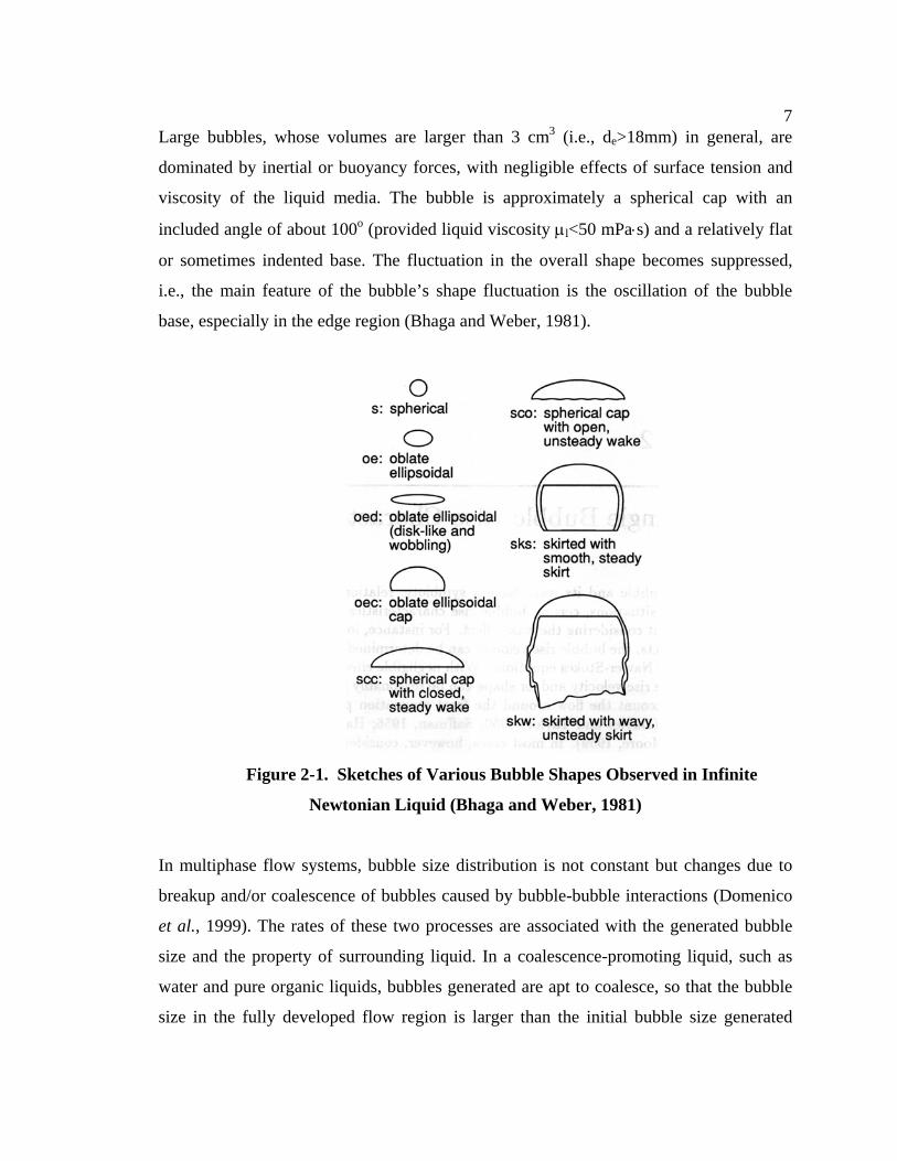
7 Large bubbles, whose volumes are larger than 3 cm3 (i.e., de>18mm) in general, are

dominated by inertial or buoyancy forces, with negligible effects of surface tension and

viscosity of the liquid media. The bubble is approximately a spherical cap with an

included angle of about 100o (provided liquid viscosity µl<50 mPa⋅s) and a relatively flat

or sometimes indented base. The fluctuation in the overall shape becomes suppressed,

i.e., the main feature of the bubble’s shape fluctuation is the oscillation of the bubble

base, especially in the edge region (Bhaga and Weber, 1981).

Figure 2-1. Sketches of Various Bubble Shapes Observed in Infinite

Newtonian Liquid (Bhaga and Weber, 1981)

In multiphase flow systems, bubble size distribution is not constant but changes due to

breakup and/or coalescence of bubbles caused by bubble-bubble interactions (Domenico

et al., 1999). The rates of these two processes are associated with the generated bubble

size and the property of surrounding liquid. In a coalescence-promoting liquid, such as

water and pure organic liquids, bubbles generated are apt to coalesce, so that the bubble

size in the fully developed flow region is larger than the initial bubble size generated

8from the sparger. When a coalescence hindering liquid, such as electrolytes and alcohols,

are added to an aqueous solution, the initial bubbles generated at the sparger essentially

do not change in size in the course of rising to the free surface. Accordingly, higher gas

holdup and specific interfacial area than those encountered in a coalescence-promoting

liquid can be achieved in a coalescence hindering liquid (Hikita et al., 1980; Heijnen and

van’t Riet, 1984). It has been reported that whatever the liquid phase, in multiphase flow

systems the bubble size distributions are very asymmetric and can be represented well by

the log-normal distribution (Luewisutthichat, Tsutsumi and Yoshida, 1997a;

Rajarathinam and Nafis, 1996; Chanson, 1997).

No broadly applicable model for the determination of rates of coalescence and breakup

has yet been presented, due to both the inaccurate understanding of the physical

mechanisms that lead to bubble breakup and coalescence, and the enormous difficulty in

obtaining reliable data, especially at high gas flow rates. The latter is the reason why

bubble size distribution measurements are not so common in literature, and, often,

different techniques lead to different measured values. Actually, bubble size in bubble

columns, including 2D bubble columns, cannot be measured directly, i.e., without any

assumptions on bubble shape, by any available technique so far, except at some extreme

conditions, e.g., single bubble rise or a extremely thin 2D bubble column (Spicka et al.,

1999). Methods now available to derive the bubble size distribution include:

(1) Video imaging (Bhaga and Weber, 1981; Domenico et al., 1999; Spicka et al., 1999).

(2) Point probes (Burgess and Calderbank, 1975; Manabu et al., 1995; Wu and Ishii,

1999; Sanaullah, Zaidi and Hills, 2001; Vince et al., 1982; Yu and Kim, 1988; Chabot et

al., 1992; Farag et al., 1997; Mudde and Saito, 2001; Xue et al., 2003).

(3) Dynamic gas disengagement technique (Krishna, Wilkinson and van Dierendonck,

1991; Daly, Patel and Bucker, 1992; Deshpande, Dinkar and Joshi, 1995).

9The bubble size distribution obtained by the dynamic gas disengagement method is not

reliable, due to unrealistic assumptions and too many approximations, e.g., the bubble

size is obtained from the correlation of bubble size and the terminal rise velocity in a still

medium and the bubble rise velocities were calculated very roughly (Daly, Patel and

Bukur, 1992).

Video imaging has been frequently employed to study the behavior of bubbles in bubble

columns and other gas-liquid contactors. However, it can be used only in transparent

systems, e.g., 2D systems and 3D systems with very low gas holdup. At high gas holdup,

video imaging can investigate only the near wall section. Furthermore, to employ video

imaging, the wall of the multiphase systems investigated must be made of transparent

material, i.e., glass or Plexiglas, which hinders its application to high pressure systems.

Hence, video imaging is not suitable for practical systems, which are usually 3D, with

high gas holdup and opaque walls.

Various point probes can be used in opaque systems. They can be employed at high gas

holdup and in high pressure systems. However, the model assumed for the bubble shape

is an important factor affecting the accuracy of the measurement results for the bubble

size distribution. In general the measurement by point probes requires the transformation

of bubble chord length distribution, obtained by probes, to bubble size distribution.

Usually, simple symmetric geometric models are employed to represent bubbles’ shapes.

The following axially symmetric geometric shape models were customarily used as

approximations of real bubbles:

(1) In the case of small bubbles, bubbles are modeled as spheres (Batchelor, 1967;

Harmathy, 1960).

(2) Large bubbles (e.g., over 1.5mm diameter in air-water systems) are represented as

ellipsoids with a larger horizontal than vertical dimension (Harmathy, 1960; Clark and

Turton, 1988).

10

(3) Very large bubbles, with strong wakes in liquids, are cap-shaped (Hills and Darton,

1975; Batchelor, 1967), and can be modeled as the top lesser section of an ellipsoid or

sphere (refer to Figure 2-1).

(4) In fluidized beds, the bubble shape is often termed “spherical cap” (Reuter, 1966;

Rowe and Widler, 1973), and is modeled by the top greater section of a sphere or

ellipsoid.

The shape of splitting and coalescing bubbles is very complicated. Data interpretation in

such circumstances is very difficult, for the shape is not well defined. Furthermore, in

many situations, e.g., in churn-turbulent flow, due to the bubble shape fluctuation

mentioned above, the shape of many bubbles is highly irregular and is not constant, so

that it cannot be represented by any simple geometric model at all.

In gas-liquid upflow, bubbles move faster than the surrounding liquid (due to buoyancy),

and large bubbles rise more quickly than small bubbles. The motion of bubbles is very

complex. The rise path and change in orientation of the bubble are known to be strongly

related to the bubble shape (Fan and Tsuchiya, 1990). The motion of spherical bubbles is

usually rectilinear. Once the bubble becomes deformed into an oblate ellipsoid, instability

sets in, and results in a spiral or zigzag trajectory. Luewisutthichat, Tsutsumi and Yoshida

(1997b) found that both the bubble shape and bubble velocity of oblate ellipsoidal

bubbles exhibit chaotic features. In turn, the fluctuation of the bubble shape is likely to

cause oscillation of the drag force, leading to the chaotic fluctuation of bubble velocity in

the streamwise direction. Therefore, in spite of the periodic macroscopic motion, bubbles

exhibit highly chaotic fluctuations in both the lateral and axial components along the

zigzag path of the bubble ascent. At the same time, the bubble orientation changes in

such a way that the bubble major axis tends to be perpendicular to the direction of

instantaneous motion (Haberman and Morton, 1953).

11 As the bubble size increases further, the bubble changes from an ellipsoidal to spherical-

cap shape, the radius of the spiral or the amplitude of the zigzag path gradually decreases

as bubble size increases, and the motion eventually becomes rectilinear style, but with a

oscillating component. This rule is generally valid in systems of low Morton number,

3

4gMoρσµ

= , where g is the acceleration of gravity, ρ, σ and µ are the density, surface

tension and viscosity of the liquid.

2.1.2 Gas Liquid Flow Patterns and Flow Regimes (Hydrodynamics)

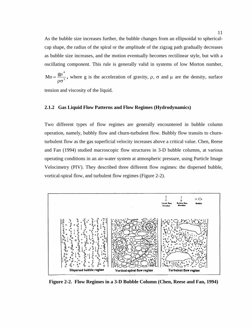
Two different types of flow regimes are generally encountered in bubble column

operation, namely, bubbly flow and churn-turbulent flow. Bubbly flow transits to churn-

turbulent flow as the gas superficial velocity increases above a critical value. Chen, Reese

and Fan (1994) studied macroscopic flow structures in 3-D bubble columns, at various

operating conditions in an air-water system at atmospheric pressure, using Particle Image

Velocimetry (PIV). They described three different flow regimes: the dispersed bubble,

vortical-spiral flow, and turbulent flow regimes (Figure 2-2).

Figure 2-2. Flow Regimes in a 3-D Bubble Column (Chen, Reese and Fan, 1994)

12 At low gas velocities, bubble streams are observed to rise rectilinearly with relatively

uniform size distribution along the column radius. Bubble coalescence and breakup are

insignificant in this dispersed bubble regime.

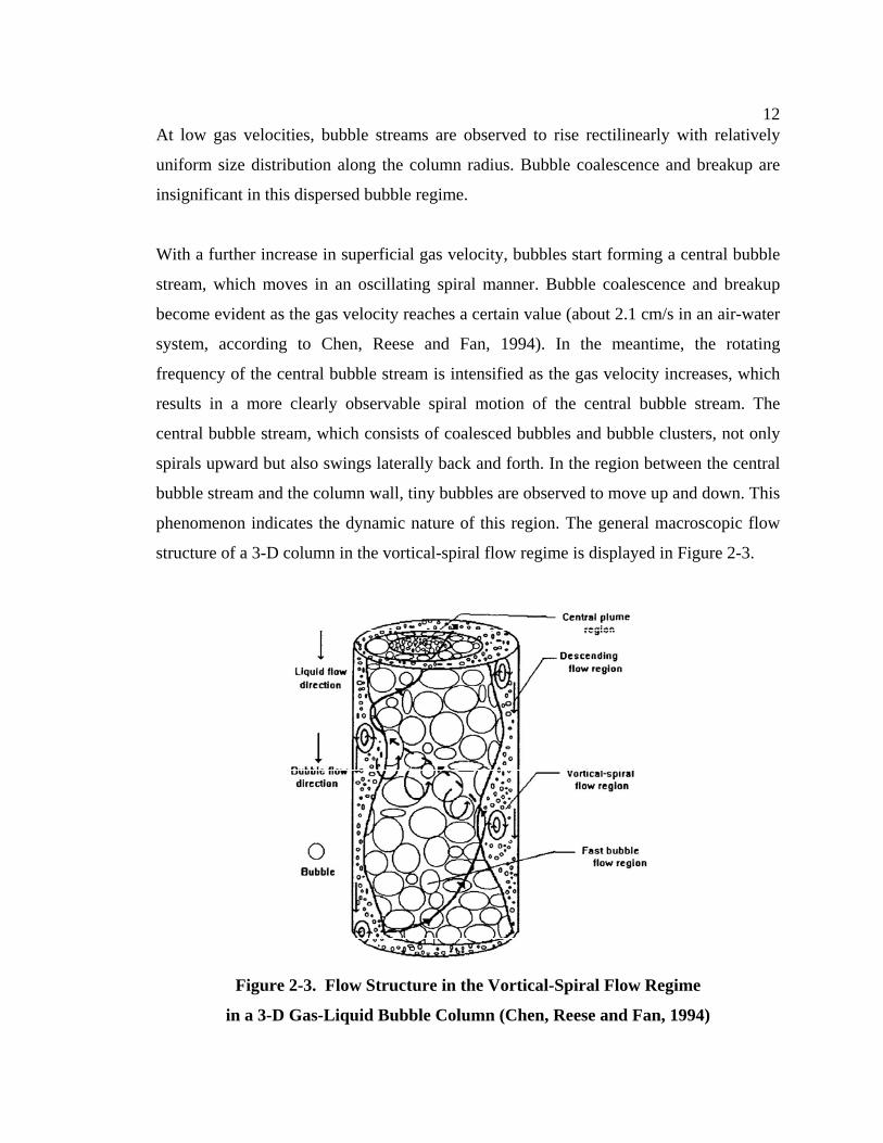
With a further increase in superficial gas velocity, bubbles start forming a central bubble

stream, which moves in an oscillating spiral manner. Bubble coalescence and breakup

become evident as the gas velocity reaches a certain value (about 2.1 cm/s in an air-water

system, according to Chen, Reese and Fan, 1994). In the meantime, the rotating

frequency of the central bubble stream is intensified as the gas velocity increases, which

results in a more clearly observable spiral motion of the central bubble stream. The

central bubble stream, which consists of coalesced bubbles and bubble clusters, not only

spirals upward but also swings laterally back and forth. In the region between the central

bubble stream and the column wall, tiny bubbles are observed to move up and down. This

phenomenon indicates the dynamic nature of this region. The general macroscopic flow

structure of a 3-D column in the vortical-spiral flow regime is displayed in Figure 2-3.

Figure 2-3. Flow Structure in the Vortical-Spiral Flow Regime

in a 3-D Gas-Liquid Bubble Column (Chen, Reese and Fan, 1994)

13

For still higher gas velocity ranges (4.2~4.9 cm/s, Chen, Reese and Fan, 1994), large

bubbles start forming by intensive bubble coalescence, and moving in a sort of “discrete”

manner, i.e., discrete large bubbles are separated by a certain distance. The spiral flow

pattern of the central bubble stream gradually breaks down.

Krishna, Wilkinson and van Dierendonck (1991) inferred from gas disengagement

experiments that there are both large and small bubbles in churn-turbulent flow; large

bubbles constitute the so-called “dilute” phase, and rise rapidly through the core of the

column, which causes the radial gas holdup profile to be almost parabolic. This non-

uniform gas holdup profile drives liquid circulation, i.e., the liquid rises in the center and

falls by the wall. The smaller bubbles form the “dense” phase and closely follow the

liquid, thereby undergoing recirculation with the liquid. Large bubbles rise fast through

the column virtually in plug flow, while small bubbles display a wide residence time

distribution. Beyond a certain transition gas velocity, the small bubble holdup remains

constant, while the large bubble holdup keeps increasing with the gas velocity. Such a

‘bimodal’ bubble size distribution is reported by Krishna, Wilkinson and van

Dierendonck (1991) as a characteristic feature of the churn-turbulent flow regime.

However, Deshpande, Dinkar and Joshi (1995) provided another explanation for the gas

disengagement experimental results. They thought that the initial faster gas

disengagement is partly due to internal liquid recirculation instead of due to only the

presence of very large bubbles, and, hence, claimed that the bimodal bubble size

distribution is not necessarily proven by results of gas disengagement experiments.

As mentioned before, the video imaging method is limited to 2D systems and 3D systems

of very low gas holdup. Fan et al. (1999) found that under high-pressure conditions

bubble coalescence is suppressed, bubble breakup is enhanced, and the distributor tends

to generate smaller bubbles. All these factors contribute to small bubble sizes and narrow

bubble size distributions. However, their observation was conducted in bubble columns

14of small diameter (2” and 4”) and at low gas holdup. Hence, there are no visual or video

observations available for 3D bubble columns, of larger size and operated at high

superficial gas velocity and high pressure, to clarify the existence or lack of the bimodal

bubble size distribution in churn-turbulent flow. By measuring the bubble chord length

distribution with a four-point optical probe in a bubble column of 6.4” diameter and at

high superficial gas velocity (up to 60 cm/s) and high pressure (up to 10 bar) in this

research, it is expected that this issue can be clarified.

2.1.3 Effect of Operating Conditions on Hydrodynamics

The superficial gas velocity is one of the most important factors that affect the

hydrodynamics in bubble columns. As the superficial gas velocity increases, the flow

condition in bubble columns changes from bubbly flow to churn-turbulent flow; at the

same time, the liquid recirculation is enhanced; the Sauter mean bubble diameter

increases, and the bubble size distribution becomes wider (Olmos et al., 2001). The gas

holdup radial profile is flat in bubbly flow, and it is parabolic in churn-turbulent flow; in

bubbly flow the gas holdup increases more rapidly with gas velocity than in churn-

turbulent flow (Chen, Reese and Fan, 1994; Kemoun et al., 2001; Lin et al., 2001).

Pressure and temperature affect the behavior of bubbles mainly by varying physical

properties of fluids (gas density, liquid viscosity, surface tension). In detail, gas density

increases with pressure and decreases with temperature, the liquid surface tension

decreases with both pressure and temperature, the liquid viscosity decreases with

temperature, and the effect of pressure on liquid viscosity is negligible.

It was found that the Sauter mean bubble diameter decreases with an increase in pressure

or temperature; the rise velocity of bubbles decreases with an increase in pressure and a

decrease in temperature (Fan et al., 1999; Lin, Tsuchiya and Fan, 1998). At elevated

pressure, the transition from bubbly flow to churn-turbulent flow is delayed (Letzel et al.,

1997). The effect of pressure on gas holdup in the homogeneous regime is insignificant

(Kolbel et al., 1961; Deckwer et al., 1980). In churn-turbulent flow, gas holdup increases

15with pressure, and the radial profile of the gas holdup becomes more parabolic (Jiang et

al., 1995; Fan et al., 1999; Chen et al., 1999b). Consequently, the volumetric mass

transfer coefficient increases also with pressure (Stegeman et al., 1996). Some

researchers (Wilkinson and Haringa, 1994; Jiang et al., 1995; Luo et al., 1998) believe

that as pressure is increased, the bubble size at the distributor is reduced; bubble

coalescence is suppressed; and large bubbles tend to break up, so that higher pressure

(gas density) leads to smaller bubbles, and hence to an increase in gas holdup. However,

in bubbly flow, this could not be confirmed by studies at Sandia National Laboratory

(Shollenberger et al., 1997). Generally an increase in temperature leads to higher gas

holdup (Bach and Pilhofer, 1978; Zou et al., 1988; Wilkinson and van Dierendonck,

1990). The reasons are: (1) Both the surface tension and the liquid viscosity decrease if

the temperature increases, and lower surface tension and liquid viscosity leads to a higher

gas holdup. (2) A higher temperature also increases the vapor pressure of the liquid. If the

feed gas to a bubble column is not saturated, the evaporation of the liquid phase can lead

to a substantial increase in the volumetric gas flow rate, which subsequently increases the

gas holdup.

It was reported that column diameters larger than about 15 cm do not affect gas holdup

much (Chen et al., 1998). On the other hand, the liquid recirculation in a large diameter

column is stronger than that in a small diameter column (Joshi et al., 1998; Chen et al.,

1998).

The gas distributor also has important effects on bubbles in bubble columns.

Jamialahmadi and Muller-Steinhagen (1993) found that in the bubbly flow regime,

bubble size was a strong function of the orifice diameter and the wettability of the gas

distributor, and a weak function of superficial gas velocity. In the churn-turbulent flow

regime, this functionality was reversed, i.e., the effect of the sparger on the gas holdup

and the liquid velocity profile is weak in the fully developed flow region in bubble

columns. Mikkilineni and Knickle (1987) studied the effect of various porous-plate gas

distributors (polyethylene, polypropylene, SiC, Al2O3, etc.) on gas holdup and flow

16pattern in the bubbly flow regime in a bubble column. They reported the following: (1)

Gas holdup increased with the pore size and distributor thickness, (2) Hydrophobic

distributor plates gave higher gas holdup than the hydrophilic ones because the

hydrophilic plates promote bubble coalescence, which results in decreased gas holdup,

due to different wetting characteristics, and (3) The bubble size was dependent on the

pore size, gas velocity, and column height and not on the distributor thickness and

material.

The situation in slurry bubble columns is more complicated. Whether a rising bubble

behaves as if it were in a “homogeneous” or “heterogeneous” medium depends primarily

on the ratio of the particle diameter to bubble diameter, i.e., the effect of solid particles on

bubble characteristics is entirely different in different particle size ranges. In case of

small particles (less than 100 µm as reported by Luewisutthichat, Tsutsumi and Yoshida,

1997), no significant difference in bubble size and velocity distribution was observed in

comparison with two-phase systems. A liquid-solid mixture of small, light particles is

often regarded as a pseudo-homogeneous medium. On the other hand, in large particle

systems (larger than 500 µm), increased bubble coalescence and breakup due to the

presence of large particles take place, resulting in a broader bubble size distribution with

larger Sauter mean diameter, causing a drop in gas holdup (Darton and Harrison, 1974;

Lee, Soria and De Lasa, 1990; Luewisutthichat, Tsutsumi and Yoshida, 1997).

2.1.4 Specific Interfacial Area

Gas-liquid mass transfer in multiphase reactors, e.g., bubble columns, is most frequently

characterized by the overall volumetric mass transfer coefficient kLa. The specific

interfacial area, a, varies significantly with the hydrodynamic conditions in reactors. For

the commonly used local two fluid models in Computational Fluid Dynamics (CFD),

prediction of the interfacial area is one of the major weaknesses. Thus, experimental data

for the distribution of interfacial area in the entire reactor are of great interest for the

validation of two fluid models, and for locating zones of low mass transfer in real

17 reactors (Kiambi et al., 2001). Furthermore, the specific interfacial area is one of the key

parameters that determine the heat and mass transfer in multiphase systems. Hence, it is

crucial for the design, simulation, and scaleup of bubble columns.

Various physical and chemical methods have been applied to measure the specific

interfacial area in multiphase flows.

The physical methods include gas disengagement (Patel, Daly and Bukur, 1990), video

imaging (Akita and Yoshida, 1974; Luewisutthichat, Tsutsumi and Yoshida, 1997; Lage

and Esposito, 1999; Pohorecki, Moniuk and Zdrojkowski, 1999), Laser Doppler

Anemometry (LDA) (Kulkarni et al., 2001), and probes (Kiambi et al., 2001; Wu and

Ishii, 1999). In all the physical methods except video imaging and some probes, the

specific interfacial area for unit of the bubble column volume, a, is determined from the

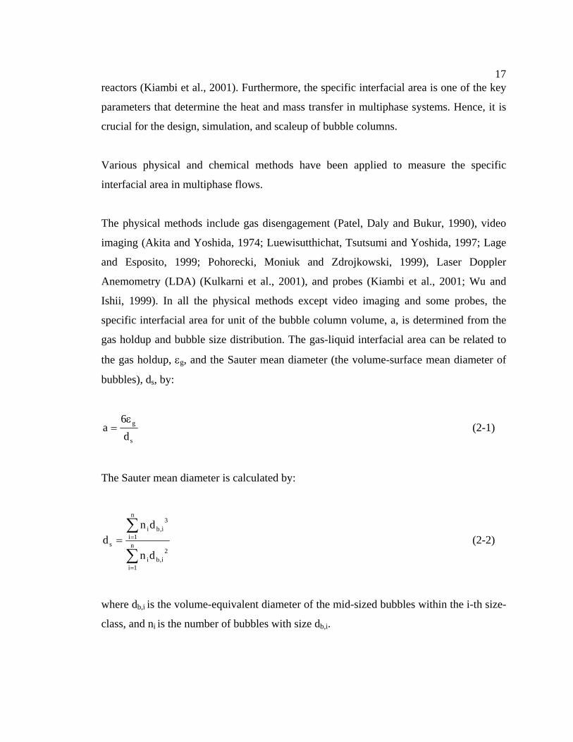
gas holdup and bubble size distribution. The gas-liquid interfacial area can be related to

the gas holdup, εg, and the Sauter mean diameter (the volume-surface mean diameter of

bubbles), ds, by:

s

g

d6

aε

= (2-1)

The Sauter mean diameter is calculated by:

∑

∑

=

== n

1i

2i,bi

n

1i

3i,bi

s

dn

dnd (2-2)

where db,i is the volume-equivalent diameter of the mid-sized bubbles within the i-th size-

class, and ni is the number of bubbles with size db,i.

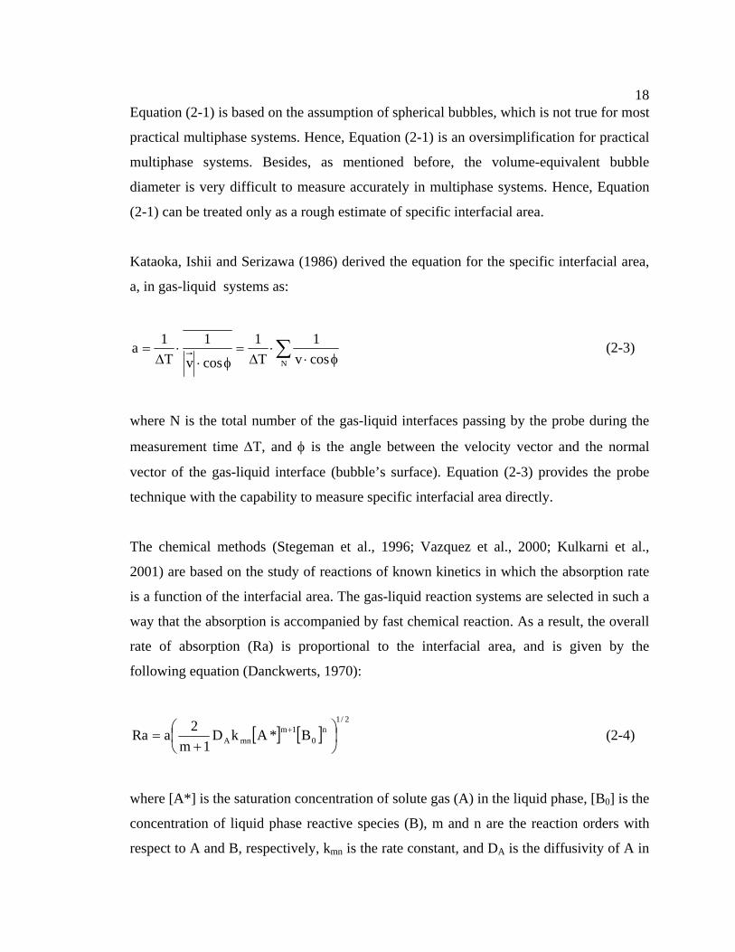
18 Equation (2-1) is based on the assumption of spherical bubbles, which is not true for most

practical multiphase systems. Hence, Equation (2-1) is an oversimplification for practical

multiphase systems. Besides, as mentioned before, the volume-equivalent bubble

diameter is very difficult to measure accurately in multiphase systems. Hence, Equation

(2-1) can be treated only as a rough estimate of specific interfacial area.

Kataoka, Ishii and Serizawa (1986) derived the equation for the specific interfacial area,

a, in gas-liquid systems as:

∑ φ⋅⋅

∆=

φ⋅⋅

∆=

N cosv1

T1

cosv

1T

1a (2-3)

where N is the total number of the gas-liquid interfaces passing by the probe during the

measurement time ∆T, and φ is the angle between the velocity vector and the normal

vector of the gas-liquid interface (bubble’s surface). Equation (2-3) provides the probe

technique with the capability to measure specific interfacial area directly.

The chemical methods (Stegeman et al., 1996; Vazquez et al., 2000; Kulkarni et al.,

2001) are based on the study of reactions of known kinetics in which the absorption rate

is a function of the interfacial area. The gas-liquid reaction systems are selected in such a

way that the absorption is accompanied by fast chemical reaction. As a result, the overall

rate of absorption (Ra) is proportional to the interfacial area, and is given by the

following equation (Danckwerts, 1970):

[ ] [ ]2/1

n0

1mmnA B*AkD

1m2aRa ⎟

⎠⎞

⎜⎝⎛

+= + (2-4)

where [A*] is the saturation concentration of solute gas (A) in the liquid phase, [B0] is the

concentration of liquid phase reactive species (B), m and n are the reaction orders with

respect to A and B, respectively, kmn is the rate constant, and DA is the diffusivity of A in

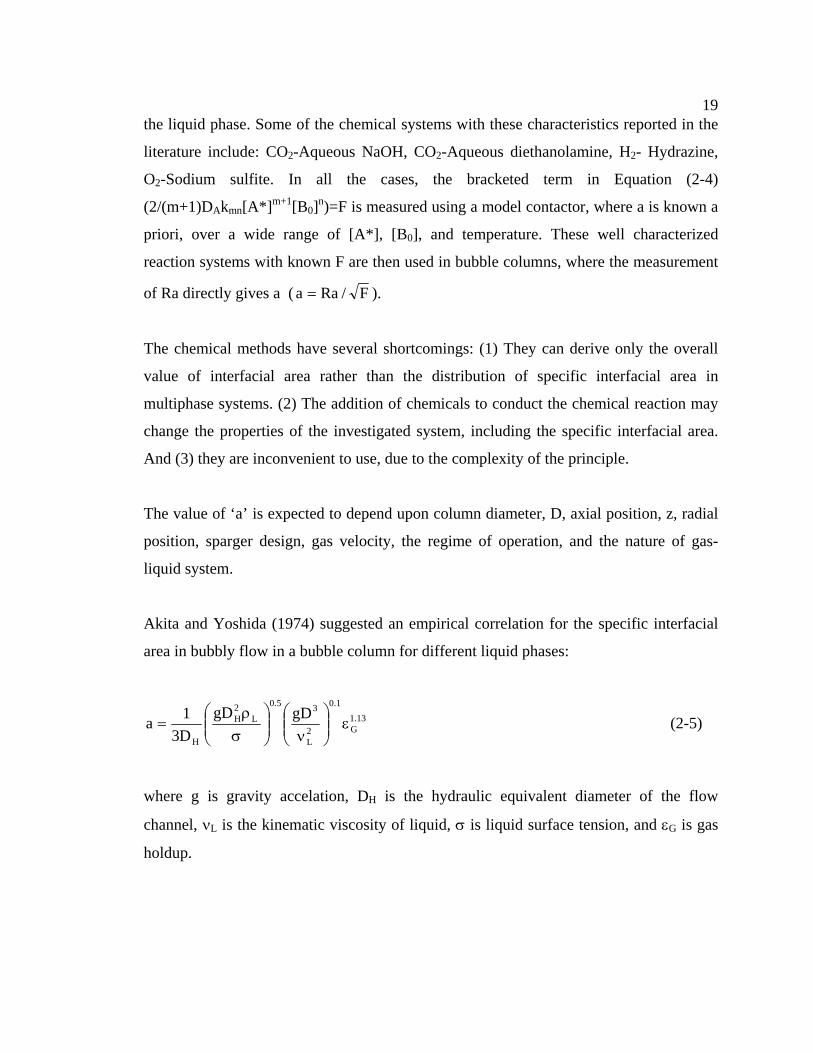
19 the liquid phase. Some of the chemical systems with these characteristics reported in the

literature include: CO2-Aqueous NaOH, CO2-Aqueous diethanolamine, H2- Hydrazine,

O2-Sodium sulfite. In all the cases, the bracketed term in Equation (2-4)

(2/(m+1)DAkmn[A*]m+1[B0]n)=F is measured using a model contactor, where a is known a

priori, over a wide range of [A*], [B0], and temperature. These well characterized

reaction systems with known F are then used in bubble columns, where the measurement

of Ra directly gives a ( F/Raa = ).

The chemical methods have several shortcomings: (1) They can derive only the overall

value of interfacial area rather than the distribution of specific interfacial area in

multiphase systems. (2) The addition of chemicals to conduct the chemical reaction may

change the properties of the investigated system, including the specific interfacial area.

And (3) they are inconvenient to use, due to the complexity of the principle.

The value of ‘a’ is expected to depend upon column diameter, D, axial position, z, radial

position, sparger design, gas velocity, the regime of operation, and the nature of gas-

liquid system.

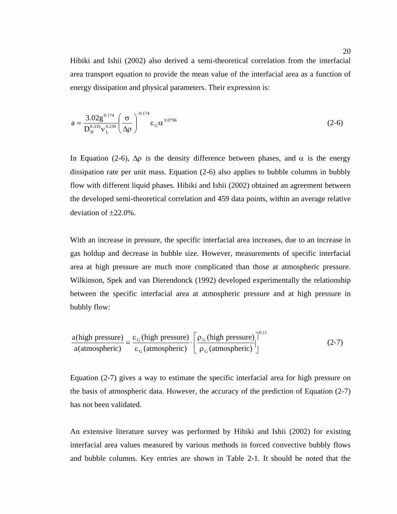
Akita and Yoshida (1974) suggested an empirical correlation for the specific interfacial

area in bubbly flow in a bubble column for different liquid phases:

13.1G

1.0

2L

35.0

L2H

H

gDgDD31a ε⎟⎟

⎠

⎞⎜⎜⎝

⎛ν⎟⎟

⎠

⎞⎜⎜⎝

⎛σρ

= (2-5)

where g is gravity accelation, DH is the hydraulic equivalent diameter of the flow

channel, νL is the kinematic viscosity of liquid, σ is liquid surface tension, and εG is gas

holdup.

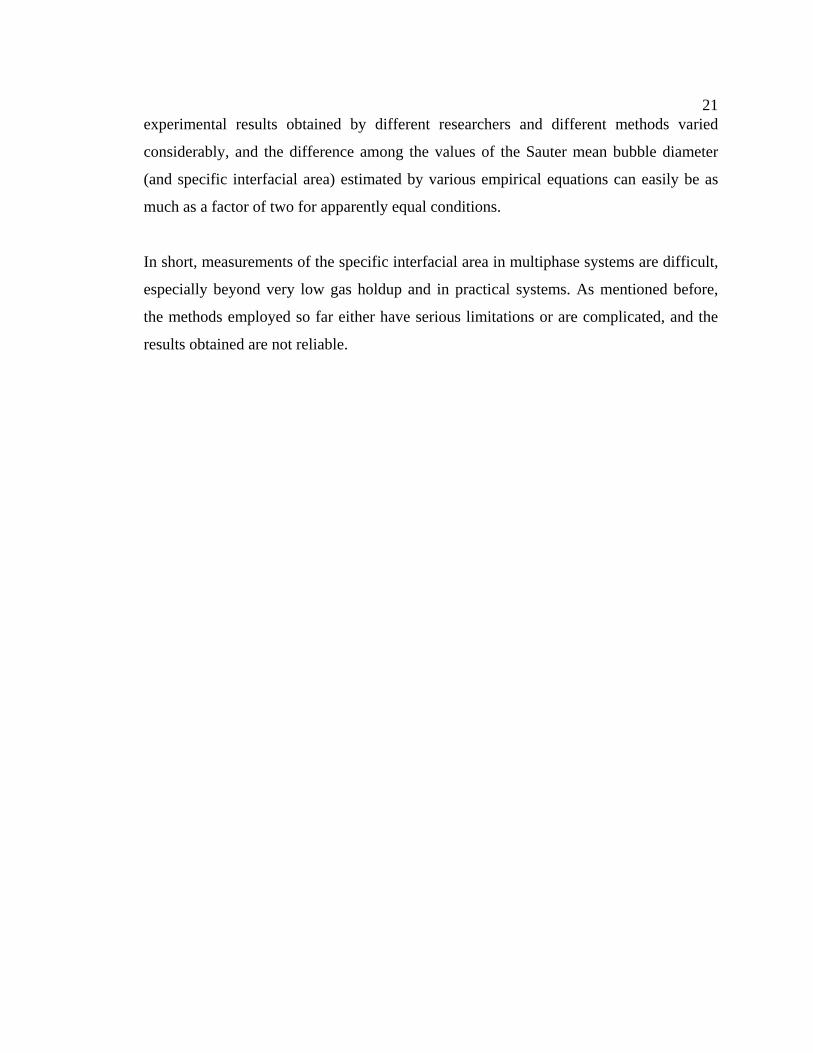
20 Hibiki and Ishii (2002) also derived a semi-theoretical correlation from the interfacial

area transport equation to provide the mean value of the interfacial area as a function of

energy dissipation and physical parameters. Their expression is:

0796.0G

174.0

239.0L

335.0H

174.0

Dg02.3a αε⎟⎟

⎠

⎞⎜⎜⎝

⎛ρ∆σ

ν=

−

(2-6)

In Equation (2-6), ∆ρ is the density difference between phases, and α is the energy

dissipation rate per unit mass. Equation (2-6) also applies to bubble columns in bubbly

flow with different liquid phases. Hibiki and Ishii (2002) obtained an agreement between

the developed semi-theoretical correlation and 459 data points, within an average relative

deviation of ±22.0%.

With an increase in pressure, the specific interfacial area increases, due to an increase in

gas holdup and decrease in bubble size. However, measurements of specific interfacial

area at high pressure are much more complicated than those at atmospheric pressure.

Wilkinson, Spek and van Dierendonck (1992) developed experimentally the relationship

between the specific interfacial area at atmospheric pressure and at high pressure in

bubbly flow:

11.0

G

G

G

G

)catmospheri()pressurehigh(

)catmospheri()pressurehigh(

)catmospheri(a)pressurehigh(a

⎥⎦

⎤⎢⎣

⎡ρρ

⋅εε

= (2-7)

Equation (2-7) gives a way to estimate the specific interfacial area for high pressure on

the basis of atmospheric data. However, the accuracy of the prediction of Equation (2-7)

has not been validated.

An extensive literature survey was performed by Hibiki and Ishii (2002) for existing

interfacial area values measured by various methods in forced convective bubbly flows

and bubble columns. Key entries are shown in Table 2-1. It should be noted that the

21experimental results obtained by different researchers and different methods varied

considerably, and the difference among the values of the Sauter mean bubble diameter

(and specific interfacial area) estimated by various empirical equations can easily be as

much as a factor of two for apparently equal conditions.

In short, measurements of the specific interfacial area in multiphase systems are difficult,

especially beyond very low gas holdup and in practical systems. As mentioned before,

the methods employed so far either have serious limitations or are complicated, and the

results obtained are not reliable.

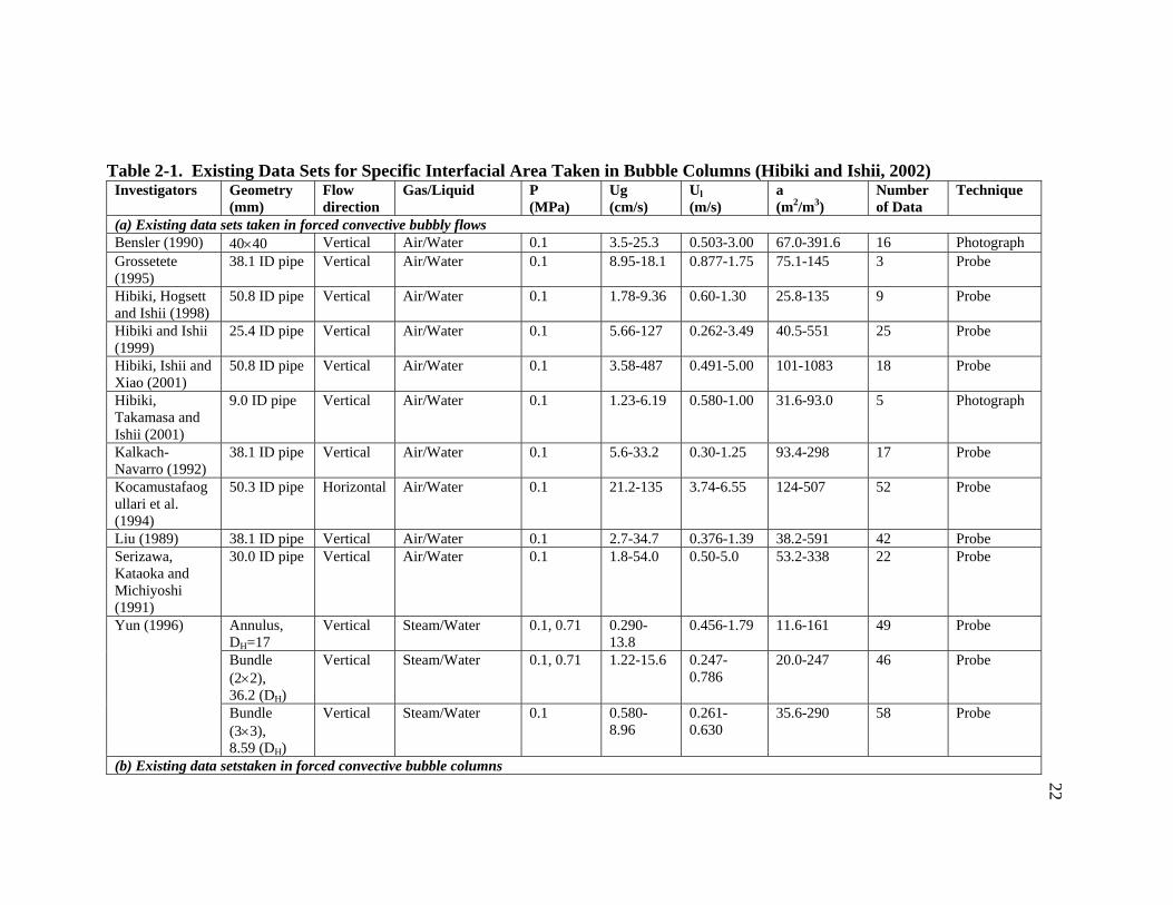
Table 2-1. Existing Data Sets for Specific Interfacial Area Taken in Bubble Columns (Hibiki and Ishii, 2002) Investigators Geometry

(mm) Flow direction

Gas/Liquid P(MPa)

Ug (cm/s)

Ul(m/s)

a (m2/m3)

Number of Data

Technique

(a) Existing data sets taken in forced convective bubbly flows Bensler (1990) 40×40 Vertical Air/Water 0.1 3.5-25.3 0.503-3.00 67.0-391.6 16 PhotographGrossetete (1995)

38.1 ID pipe Vertical Air/Water 0.1 8.95-18.1 0.877-1.75 75.1-145 3 Probe

Hibiki, Hogsett and Ishii (1998)


Hibiki and Ishii (1999)

25.4 ID pipe Vertical Air/Water 0.1 5.66-127 0.262-3.49 40.5-551 25 Probe

Hibiki, Ishii and Xiao (2001)

50.8 ID pipe Vertical Air/Water 0.1 3.58-487 0.491-5.00 101-1083 18 Probe

Hibiki, Takamasa and Ishii (2001)

9.0 ID pipe Vertical Air/Water 0.1 1.23-6.19 0.580-1.00 31.6-93.0 5 Photograph

Kalkach-Navarro (1992)


Kocamustafaogullari et al. (1994)

50.3 ID pipe Horizontal Air/Water 0.1 21.2-135 3.74-6.55 124-507 52 Probe

Liu (1989) 38.1 ID pipe Vertical Air/Water 0.1 2.7-34.7 0.376-1.39 38.2-591 42 Probe Serizawa, Kataoka and Michiyoshi (1991)


Annulus, DH=17

Vertical Steam/Water 0.1, 0.71 0.290-13.8

0.456-1.79 11.6-161 49 Probe

Bundle (2×2), 36.2 (DH)

Vertical Steam/Water 0.1, 0.71 1.22-15.6 0.247-0.786

20.0-247 46 Probe

Yun (1996)

Bundle (3×3), 8.59 (DH)

Vertical Steam/Water 0.1 0.580-8.96

0.261-0.630

35.6-290 58 Probe

(b) Existing data setstaken in forced convective bubble columns

22

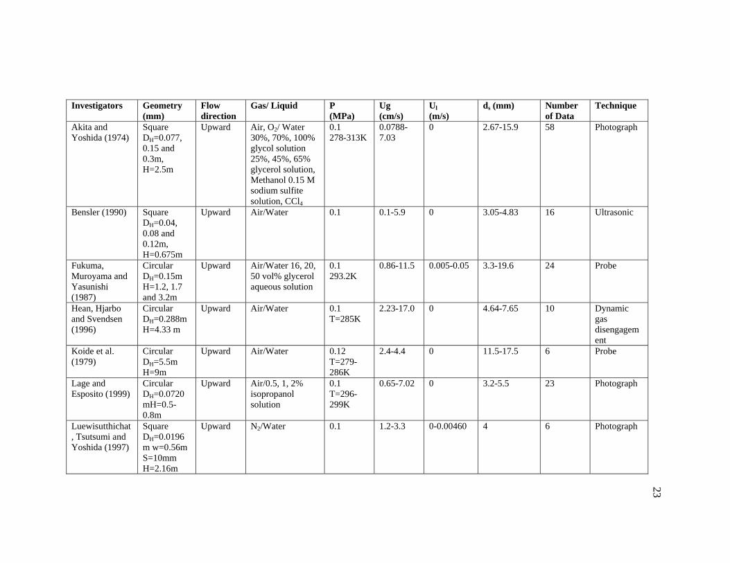
Investigators Geometry(mm)

Flow direction

Gas/ Liquid P (MPa)

Ug (cm/s)

Ul(m/s)

ds (mm) Number of Data

Technique

Akita and Yoshida (1974)

Square DH=0.077, 0.15 and 0.3m, H=2.5m

Upward Air, O2/ Water 30%, 70%, 100% glycol solution 25%, 45%, 65% glycerol solution, Methanol 0.15 M sodium sulfite solution, CCl4

0.1 278-313K

0.0788-7.03

0 2.67-15.9 58 Photograph

Bensler (1990) Square DH=0.04, 0.08 and 0.12m, H=0.675m

Upward Air/Water 0.1 0.1-5.9 0 3.05-4.83 16 Ultrasonic

Fukuma, Muroyama and Yasunishi (1987)

Circular DH=0.15m H=1.2, 1.7 and 3.2m

Upward Air/Water 16, 20,50 vol% glycerol aqueous solution

0.1 293.2K

0.86-11.5 0.005-0.05 3.3-19.6 24 Probe

Hean, Hjarbo and Svendsen (1996)

Circular DH=0.288m H=4.33 m

Upward Air/Water 0.1T=285K

2.23-17.0 0 4.64-7.65 10 Dynamicgas disengagement

Koide et al. (1979)

Circular DH=5.5m H=9m

Upward Air/Water 0.12T=279-286K

2.4-4.4 0 11.5-17.5 6 Probe

Lage and Esposito (1999)

Circular DH=0.0720mH=0.5-0.8m

Upward Air/0.5, 1, 2% isopropanol solution

0.1 T=296-299K

0.65-7.02 0 3.2-5.5 23 Photograph

Luewisutthichat, Tsutsumi and Yoshida (1997)

Square DH=0.0196m w=0.56m S=10mm H=2.16m

Upward N2/Water 0.1 1.2-3.3 0-0.00460 4 6 Photograph

23

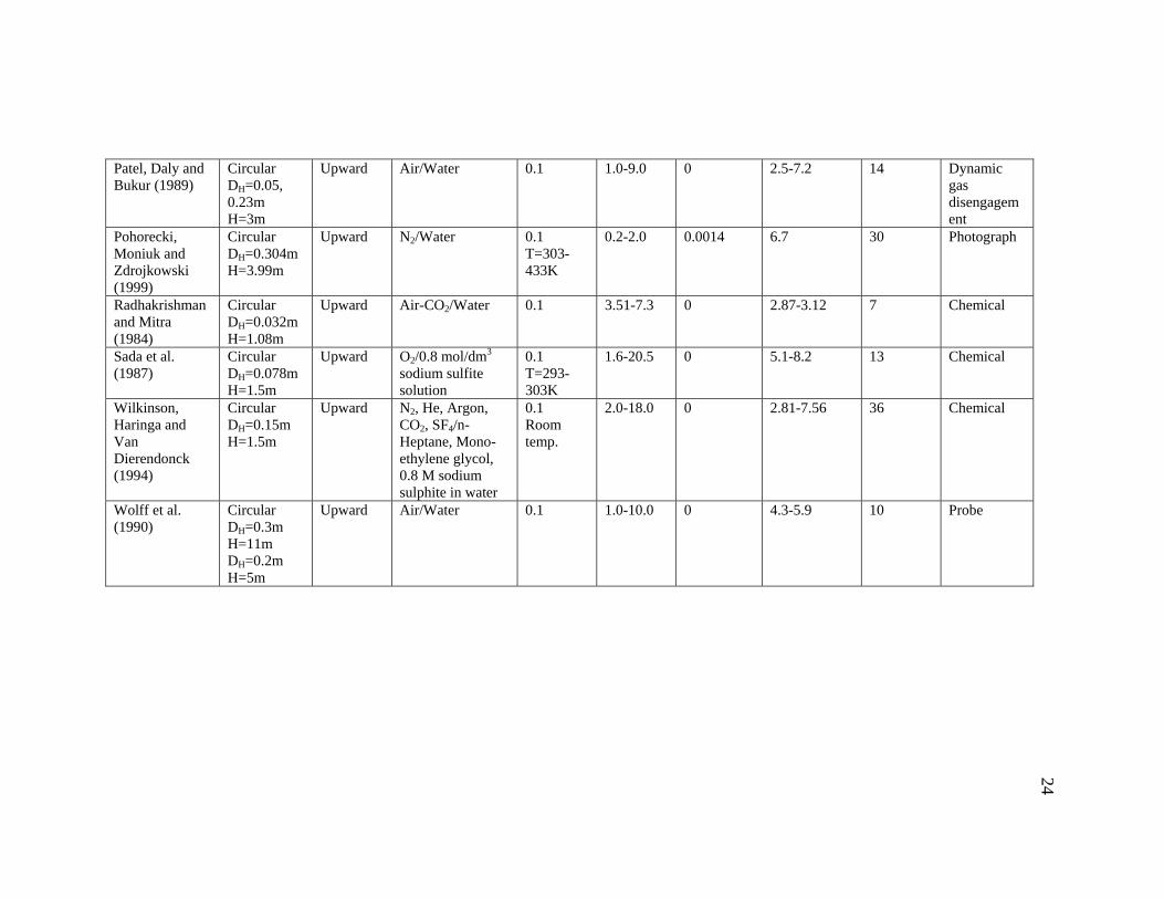
Patel, Daly and Bukur (1989)

Circular DH=0.05, 0.23m H=3m

Upward Air/Water 0.1 1.0-9.0 0 2.5-7.2 14 Dynamicgas disengagement

Pohorecki, Moniuk and Zdrojkowski (1999)

Circular DH=0.304m H=3.99m

Upward N2/Water 0.1T=303-433K

0.2-2.0 0.0014 6.7 30 Photograph

Radhakrishman and Mitra (1984)


Upward Air-CO2/Water 0.1 3.51-7.3 0 2.87-3.12 7 Chemical

Sada et al. (1987)


Upward O2/0.8 mol/dm3 sodium sulfite solution

0.1 T=293-303K

1.6-20.5 0 5.1-8.2 13 Chemical

Wilkinson, Haringa and Van Dierendonck (1994)


Upward N2, He, Argon, CO2, SF4/n-Heptane, Mono-ethylene glycol, 0.8 M sodium sulphite in water

0.1 Room temp.

2.0-18.0 0 2.81-7.56 36 Chemical

Wolff et al. (1990)

Circular DH=0.3m H=11m DH=0.2m H=5m

Upward Air/Water 0.1 1.0-10.0 0 4.3-5.9 10 Probe

24

252.2 Type of Probes Used in Multiphase Systems

In recent years, measurements of bubble behavior have usually been carried out by

various types of probes (Burgess and Calderbank, 1975; Manabu et al., 1995; Wu and

Ishii, 1999; Sanaullah, Zaidi and Hills, 2001; Vince et al., 1982; Yu and Kim, 1988;

Chabot et al., 1992; Farag et al., 1997; Mudde and Saito, 2001). The miniaturization of

probes using fiber optics or small electrodes makes them good choices for performing

direct measurements of the bubble velocity and bubble chord length, even at high gas

flow rates or in opaque systems. A comparison of measurement methods based on

miniature optical and conductivity probes was presented by Choi and Lee (1990). In

comparison with conductivity probes, optical probes offer several advantages: (1) They

can be used in conductive as well as non-conductive (organic) systems, which are

important in the petrochemical industry. (2) The presence of a liquid film on the sensor

tip reduces the effectiveness of a conductivity probe but not that of an optical probe, The

sensitivity of optical probes is therefore higher than that of conductivity probes (van der

Lans, 1985). (3) The optical probe achieves a much better signal/noise ratio than a

conductivity probe.

To measure the bubble velocity, at least two probes (tips or measure points) are needed.

The two probes (or tips, measure points) are placed in the macroscopic flow direction at a

small distance apart (e.g., 2~3 mm). The bubble velocity is calculated by dividing the

distance between these two probes by the time interval that the bubble takes to pass

through the distance between them. The two-point probes used by various researchers

have different configurations, as shown in Figure 2-4.

Mohamed

Highlight

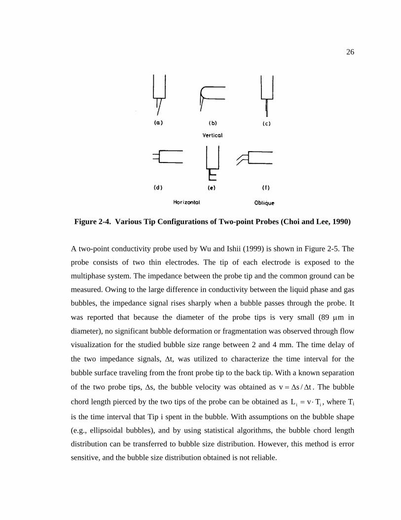
26

Figure 2-4. Various Tip Configurations of Two-point Probes (Choi and Lee, 1990)

A two-point conductivity probe used by Wu and Ishii (1999) is shown in Figure 2-5. The

probe consists of two thin electrodes. The tip of each electrode is exposed to the

multiphase system. The impedance between the probe tip and the common ground can be

measured. Owing to the large difference in conductivity between the liquid phase and gas

bubbles, the impedance signal rises sharply when a bubble passes through the probe. It

was reported that because the diameter of the probe tips is very small (89 µm in

diameter), no significant bubble deformation or fragmentation was observed through flow

visualization for the studied bubble size range between 2 and 4 mm. The time delay of

the two impedance signals, ∆t, was utilized to characterize the time interval for the

bubble surface traveling from the front probe tip to the back tip. With a known separation

of the two probe tips, ∆s, the bubble velocity was obtained as . The bubble

chord length pierced by the two tips of the probe can be obtained as , where T

t/sv ∆∆=

ii TvL ⋅= i

is the time interval that Tip i spent in the bubble. With assumptions on the bubble shape

(e.g., ellipsoidal bubbles), and by using statistical algorithms, the bubble chord length

distribution can be transferred to bubble size distribution. However, this method is error

sensitive, and the bubble size distribution obtained is not reliable.

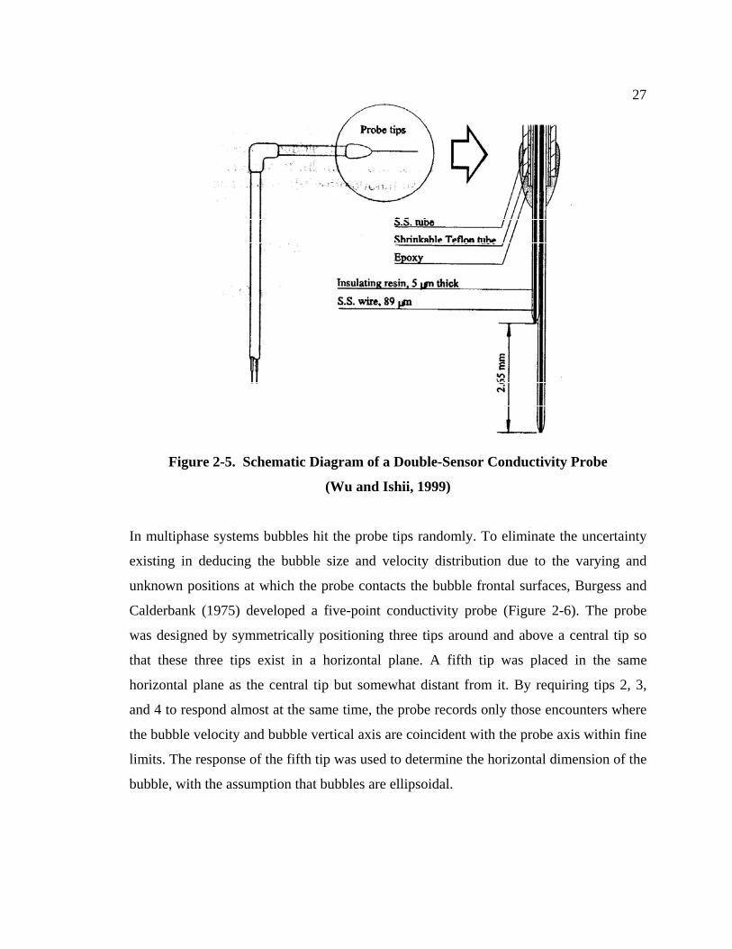
27

Figure 2-5. Schematic Diagram of a Double-Sensor Conductivity Probe

(Wu and Ishii, 1999)

In multiphase systems bubbles hit the probe tips randomly. To eliminate the uncertainty

existing in deducing the bubble size and velocity distribution due to the varying and

unknown positions at which the probe contacts the bubble frontal surfaces, Burgess and

Calderbank (1975) developed a five-point conductivity probe (Figure 2-6). The probe

was designed by symmetrically positioning three tips around and above a central tip so

that these three tips exist in a horizontal plane. A fifth tip was placed in the same

horizontal plane as the central tip but somewhat distant from it. By requiring tips 2, 3,

and 4 to respond almost at the same time, the probe records only those encounters where

the bubble velocity and bubble vertical axis are coincident with the probe axis within fine

limits. The response of the fifth tip was used to determine the horizontal dimension of the

bubble, with the assumption that bubbles are ellipsoidal.

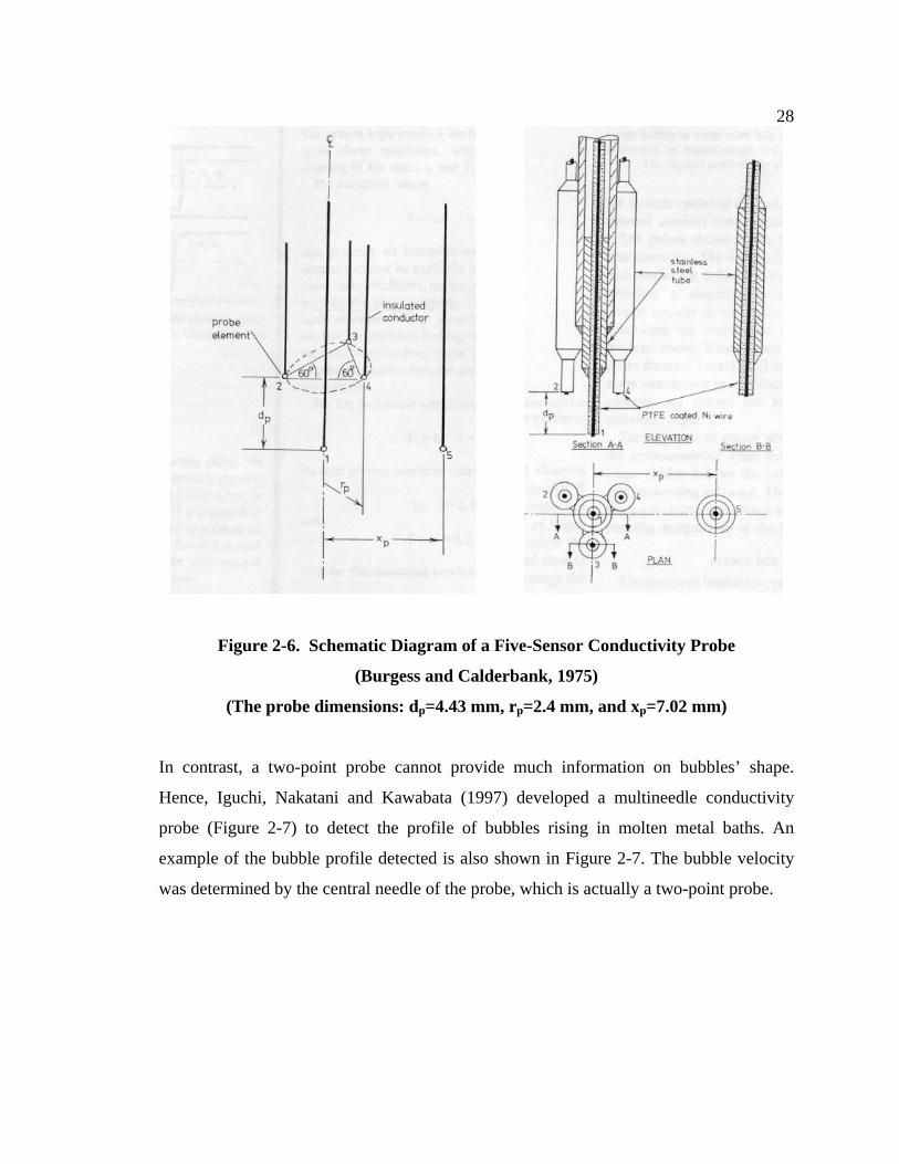
28

Figure 2-6. Schematic Diagram of a Five-Sensor Conductivity Probe

(Burgess and Calderbank, 1975)

(The probe dimensions: dp=4.43 mm, rp=2.4 mm, and xp=7.02 mm)

In contrast, a two-point probe cannot provide much information on bubbles’ shape.

Hence, Iguchi, Nakatani and Kawabata (1997) developed a multineedle conductivity

probe (Figure 2-7) to detect the profile of bubbles rising in molten metal baths. An

example of the bubble profile detected is also shown in Figure 2-7. The bubble velocity

was determined by the central needle of the probe, which is actually a two-point probe.

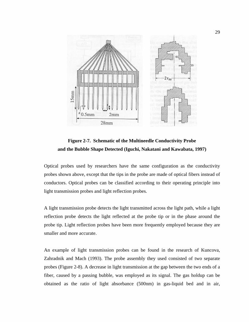
29

Figure 2-7. Schematic of the Multineedle Conductivity Probe

and the Bubble Shape Detected (Iguchi, Nakatani and Kawabata, 1997)

Optical probes used by researchers have the same configuration as the conductivity

probes shown above, except that the tips in the probe are made of optical fibers instead of

conductors. Optical probes can be classified according to their operating principle into

light transmission probes and light reflection probes.

A light transmission probe detects the light transmitted across the light path, while a light

reflection probe detects the light reflected at the probe tip or in the phase around the

probe tip. Light reflection probes have been more frequently employed because they are

smaller and more accurate.

An example of light transmission probes can be found in the research of Kuncova,

Zahradnik and Mach (1993). The probe assembly they used consisted of two separate

probes (Figure 2-8). A decrease in light transmission at the gap between the two ends of a

fiber, caused by a passing bubble, was employed as its signal. The gas holdup can be

obtained as the ratio of light absorbance (500nm) in gas-liquid bed and in air,

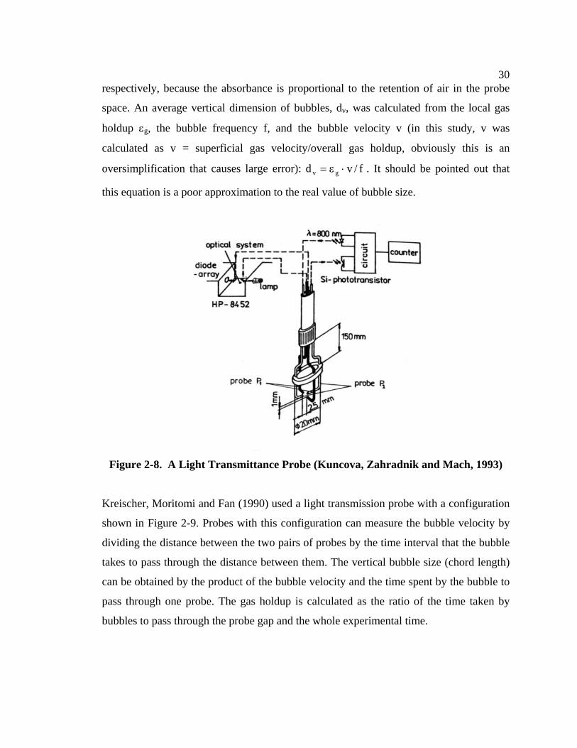
30 respectively, because the absorbance is proportional to the retention of air in the probe

space. An average vertical dimension of bubbles, dv, was calculated from the local gas

holdup εg, the bubble frequency f, and the bubble velocity v (in this study, v was

calculated as v = superficial gas velocity/overall gas holdup, obviously this is an

oversimplification that causes large error): f/vd gv ⋅ε= . It should be pointed out that

this equation is a poor approximation to the real value of bubble size.

Figure 2-8. A Light Transmittance Probe (Kuncova, Zahradnik and Mach, 1993)

Kreischer, Moritomi and Fan (1990) used a light transmission probe with a configuration

shown in Figure 2-9. Probes with this configuration can measure the bubble velocity by

dividing the distance between the two pairs of probes by the time interval that the bubble

takes to pass through the distance between them. The vertical bubble size (chord length)

can be obtained by the product of the bubble velocity and the time spent by the bubble to

pass through one probe. The gas holdup is calculated as the ratio of the time taken by

bubbles to pass through the probe gap and the whole experimental time.

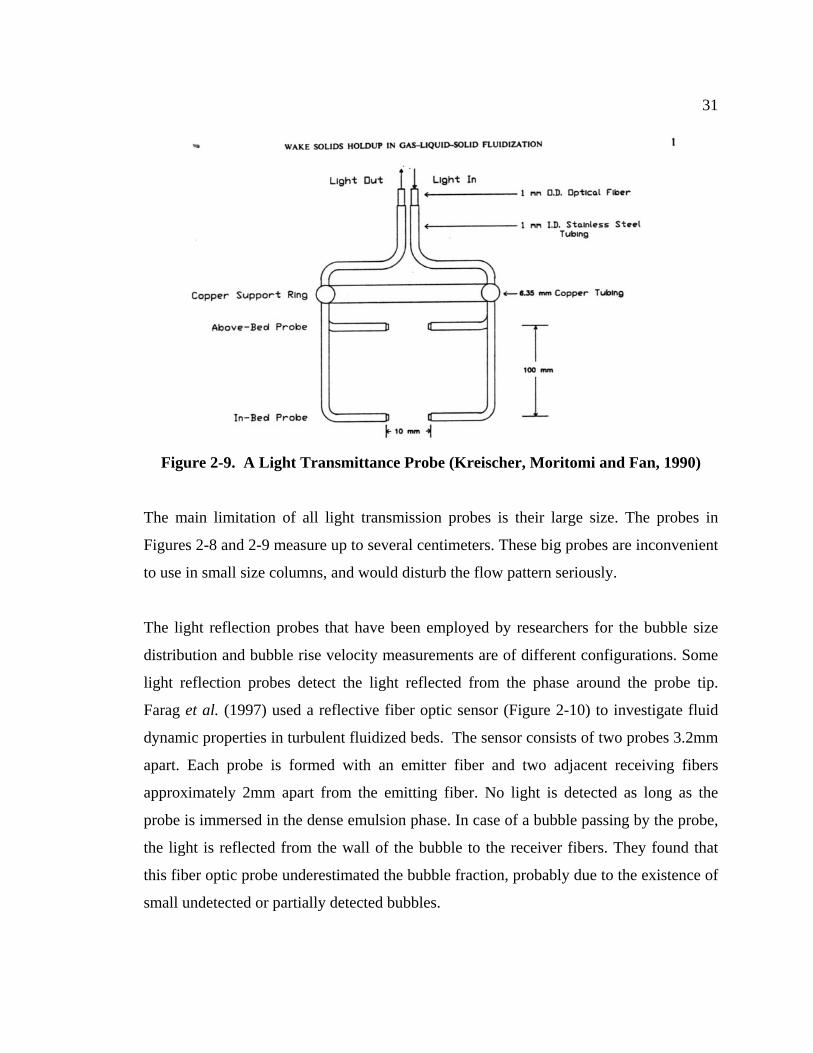
31

Figure 2-9. A Light Transmittance Probe (Kreischer, Moritomi and Fan, 1990)

The main limitation of all light transmission probes is their large size. The probes in

Figures 2-8 and 2-9 measure up to several centimeters. These big probes are inconvenient

to use in small size columns, and would disturb the flow pattern seriously.

The light reflection probes that have been employed by researchers for the bubble size

distribution and bubble rise velocity measurements are of different configurations. Some

light reflection probes detect the light reflected from the phase around the probe tip.

Farag et al. (1997) used a reflective fiber optic sensor (Figure 2-10) to investigate fluid

dynamic properties in turbulent fluidized beds. The sensor consists of two probes 3.2mm

apart. Each probe is formed with an emitter fiber and two adjacent receiving fibers

approximately 2mm apart from the emitting fiber. No light is detected as long as the

probe is immersed in the dense emulsion phase. In case of a bubble passing by the probe,

the light is reflected from the wall of the bubble to the receiver fibers. They found that

this fiber optic probe underestimated the bubble fraction, probably due to the existence of

small undetected or partially detected bubbles.

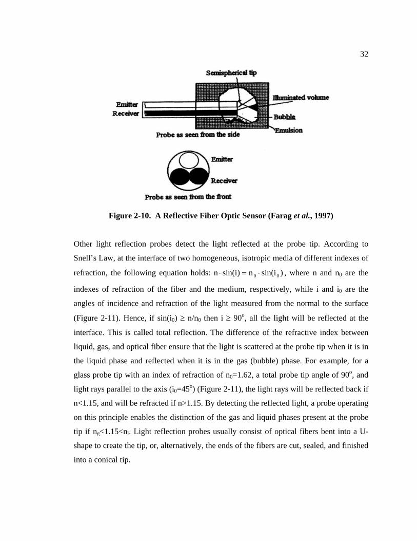
32

Figure 2-10. A Reflective Fiber Optic Sensor (Farag et al., 1997)

Other light reflection probes detect the light reflected at the probe tip. According to

Snell’s Law, at the interface of two homogeneous, isotropic media of different indexes of

refraction, the following equation holds: )isin(n)isin(n 00 ⋅=⋅ , where n and n0 are the

indexes of refraction of the fiber and the medium, respectively, while i and i0 are the

angles of incidence and refraction of the light measured from the normal to the surface

(Figure 2-11). Hence, if sin(i0) ≥ n/n0 then i ≥ 90o, all the light will be reflected at the

interface. This is called total reflection. The difference of the refractive index between

liquid, gas, and optical fiber ensure that the light is scattered at the probe tip when it is in

the liquid phase and reflected when it is in the gas (bubble) phase. For example, for a

glass probe tip with an index of refraction of n0=1.62, a total probe tip angle of 90o, and

light rays parallel to the axis (i0=45o) (Figure 2-11), the light rays will be reflected back if

n<1.15, and will be refracted if n>1.15. By detecting the reflected light, a probe operating

on this principle enables the distinction of the gas and liquid phases present at the probe

tip if ng<1.15<nl. Light reflection probes usually consist of optical fibers bent into a U-

shape to create the tip, or, alternatively, the ends of the fibers are cut, sealed, and finished

into a conical tip.

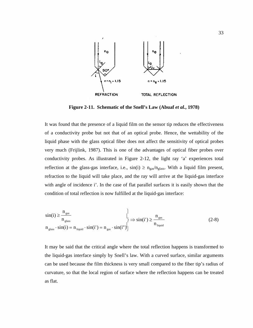
33

Figure 2-11. Schematic of the Snell’s Law (Abuaf et al., 1978)

It was found that the presence of a liquid film on the sensor tip reduces the effectiveness

of a conductivity probe but not that of an optical probe. Hence, the wettability of the

liquid phase with the glass optical fiber does not affect the sensitivity of optical probes

very much (Frijlink, 1987). This is one of the advantages of optical fiber probes over

conductivity probes. As illustrated in Figure 2-12, the light ray ‘a’ experiences total

reflection at the glass-gas interface, i.e., sin(i) ≥ ngas/nglass. With a liquid film present,

refraction to the liquid will take place, and the ray will arrive at the liquid-gas interface

with angle of incidence i’. In the case of flat parallel surfaces it is easily shown that the

condition of total reflection is now fulfilled at the liquid-gas interface:

liquid

gas

gasliquidglass

glass

gas

nn

)'isin()"isin(n)'isin(n)isin(n

nn

)isin(≥⇒

⎪⎭

⎪⎬

⎫

⋅=⋅=⋅

≥ (2-8)

It may be said that the critical angle where the total reflection happens is transformed to

the liquid-gas interface simply by Snell’s law. With a curved surface, similar arguments

can be used because the film thickness is very small compared to the fiber tip’s radius of

curvature, so that the local region of surface where the reflection happens can be treated

as flat.

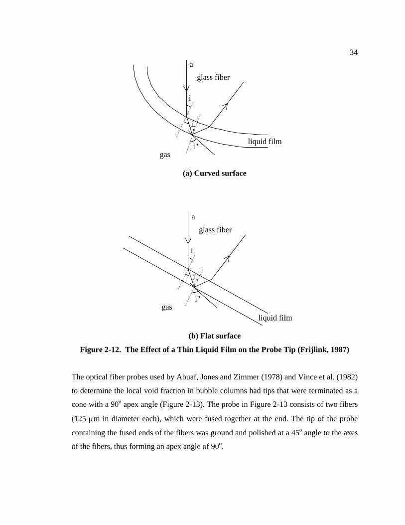
34

liquid film

glass fiber

i

a

gasi"

i'

(a) Curved surface

liquid film

glass fiber

i

a

gasi"

i'

(b) Flat surface

Figure 2-12. The Effect of a Thin Liquid Film on the Probe Tip (Frijlink, 1987)

The optical fiber probes used by Abuaf, Jones and Zimmer (1978) and Vince et al. (1982)

to determine the local void fraction in bubble columns had tips that were terminated as a

cone with a 90o apex angle (Figure 2-13). The probe in Figure 2-13 consists of two fibers

(125 µm in diameter each), which were fused together at the end. The tip of the probe

containing the fused ends of the fibers was ground and polished at a 45o angle to the axes

of the fibers, thus forming an apex angle of 90o.

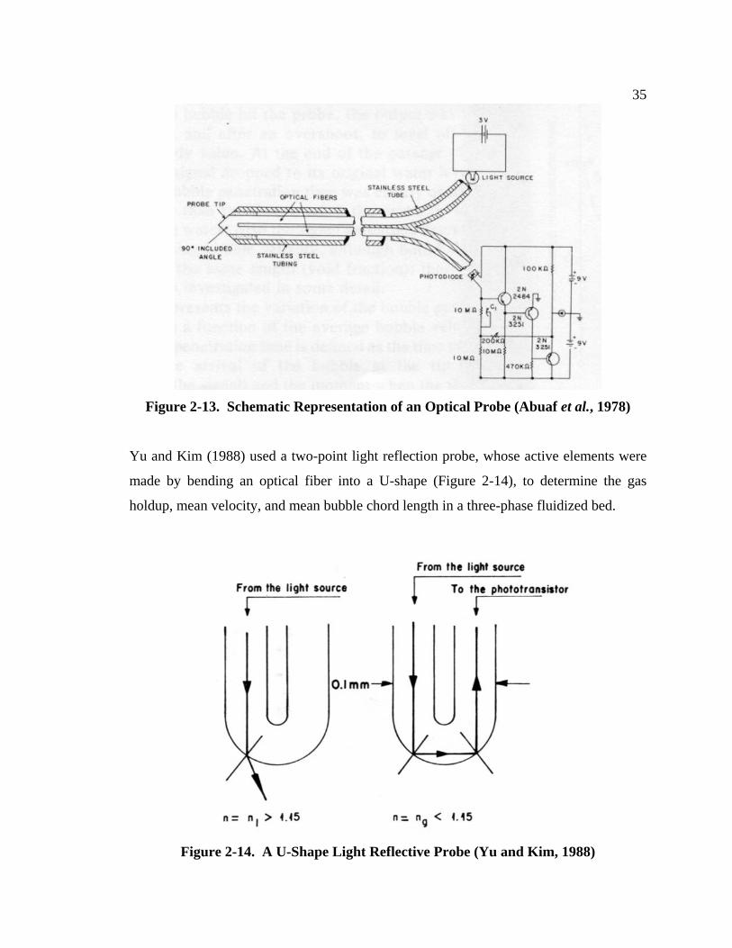
35

Figure 2-13. Schematic Representation of an Optical Probe (Abuaf et al., 1978)

Yu and Kim (1988) used a two-point light reflection probe, whose active elements were

made by bending an optical fiber into a U-shape (Figure 2-14), to determine the gas

holdup, mean velocity, and mean bubble chord length in a three-phase fluidized bed.

Figure 2-14. A U-Shape Light Reflective Probe (Yu and Kim, 1988)

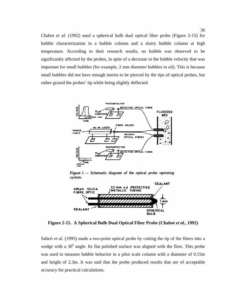
36 Chabot et al. (1992) used a spherical bulb dual optical fiber probe (Figure 2-15) for

bubble characterization in a bubble column and a slurry bubble column at high

temperature. According to their research results, no bubble was observed to be

significantly affected by the probes, in spite of a decrease in the bubble velocity that was

important for small bubbles (for example, 2 mm diameter bubbles in oil). This is because

small bubbles did not have enough inertia to be pierced by the tips of optical probes, but

rather grazed the probes’ tip while being slightly deflected.

Figure 2-15. A Spherical Bulb Dual Optical Fiber Probe (Chabot et al., 1992)

Saberi et al. (1995) made a two-point optical probe by cutting the tip of the fibers into a

wedge with a 30o angle. Its flat polished surface was aligned with the flow. This probe

was used to measure bubble behavior in a pilot scale column with a diameter of 0.15m

and height of 2.3m. It was said that the probe produced results that are of acceptable

accuracy for practical calculations.

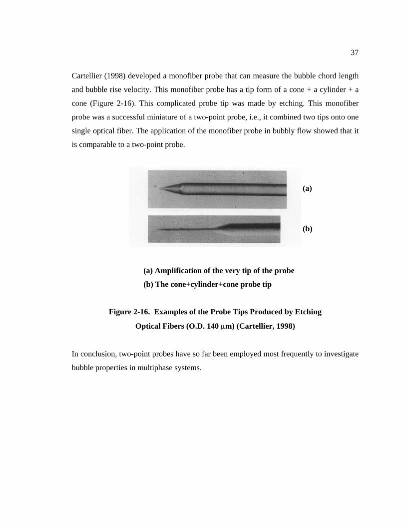
37

Cartellier (1998) developed a monofiber probe that can measure the bubble chord length

and bubble rise velocity. This monofiber probe has a tip form of a cone + a cylinder + a

cone (Figure 2-16). This complicated probe tip was made by etching. This monofiber

probe was a successful miniature of a two-point probe, i.e., it combined two tips onto one

single optical fiber. The application of the monofiber probe in bubbly flow showed that it

is comparable to a two-point probe.

(a)

(b)

(a) Amplification of the very tip of the probe

(b) The cone+cylinder+cone probe tip

Figure 2-16. Examples of the Probe Tips Produced by Etching

Optical Fibers (O.D. 140 µm) (Cartellier, 1998)

In conclusion, two-point probes have so far been employed most frequently to investigate

bubble properties in multiphase systems.

38

Chapter 3 Suggested Algorithm for the

Four-Point Optical Probe

3.1 Analysis of Measurement Errors for Two-Point Probes

As mentioned earlier, probes are the only means that can be applied in practical bubble

columns to study bubble behavior, e.g., bubble velocity and bubble chord length. Two-

point probes have been employed in most of the reported studies (Choi and Lee, 1990;

Chabot et al., 1992; Wu and Ishii, 1999; Fan et al., 1999; Magaud et al., 2001). Lim and

Agarwal (1992) analyzed the errors in bubble velocity and bubble chord length obtained

by two-point probes, based on the assumption of spherical bubbles. They found that the

relative error in the bubble velocity obtained by two-point probes varied with the

incidence angle and the position at which the bubble hits the probe. The error can easily

be over 100% in many cases. Hence, they concluded that values of both bubble velocity

and bubble chord length obtained by a two-point probe are theoretically questionable, and

experimental results reported using these probes must be viewed at best as qualitative.

However, their analysis is limited to spherical bubbles only, and did not consider the

curvature correction. Since most bubbles in bubble columns are approximately

ellipsoidal, the case of ellipsoidal bubbles is analyzed in this work, and a curvature

correction is included in the error analysis. It is thus quantitatively shown that

measurements of bubble velocity and bubble chord length by two-point probes can be

highly inaccurate. To analyze the measurement errors of two-point probes, the following

assumptions are made (refer to Figure 3-1):

(1) The bubble velocity vector aligns with the bubble orientation. In other words, the

bubble has a symmetry plane (e.g., spherical or ellipsoidal bubbles) that is perpendicular

to the bubble velocity vector.

Mohamed

Highlight

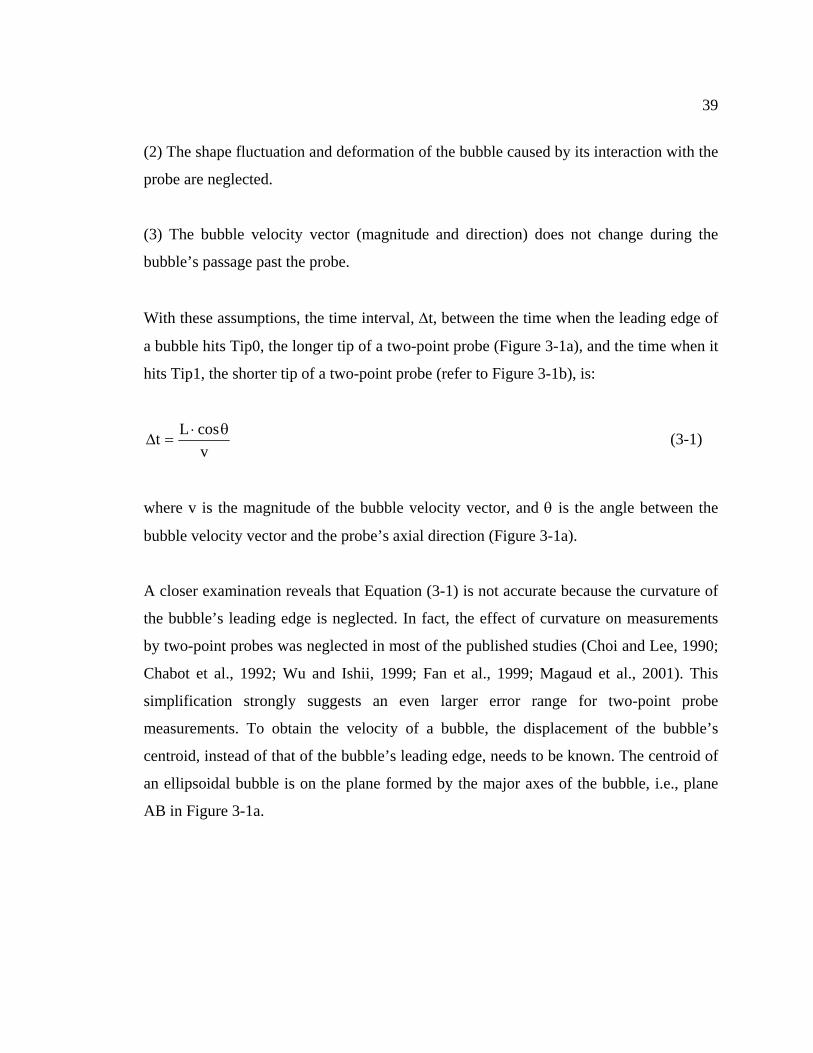
39

(2) The shape fluctuation and deformation of the bubble caused by its interaction with the

probe are neglected.

(3) The bubble velocity vector (magnitude and direction) does not change during the

bubble’s passage past the probe.

With these assumptions, the time interval, ∆t, between the time when the leading edge of

a bubble hits Tip0, the longer tip of a two-point probe (Figure 3-1a), and the time when it

hits Tip1, the shorter tip of a two-point probe (refer to Figure 3-1b), is:

vcosLt θ⋅

=∆ (3-1)

where v is the magnitude of the bubble velocity vector, and θ is the angle between the

bubble velocity vector and the probe’s axial direction (Figure 3-1a).

A closer examination reveals that Equation (3-1) is not accurate because the curvature of

the bubble’s leading edge is neglected. In fact, the effect of curvature on measurements

by two-point probes was neglected in most of the published studies (Choi and Lee, 1990;

Chabot et al., 1992; Wu and Ishii, 1999; Fan et al., 1999; Magaud et al., 2001). This

simplification strongly suggests an even larger error range for two-point probe

measurements. To obtain the velocity of a bubble, the displacement of the bubble’s

centroid, instead of that of the bubble’s leading edge, needs to be known. The centroid of

an ellipsoidal bubble is on the plane formed by the major axes of the bubble, i.e., plane

AB in Figure 3-1a.

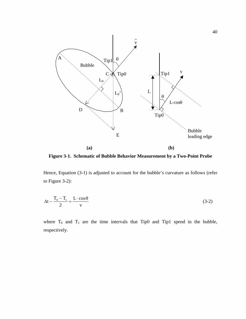
40

θ

v

Tip1

Tip0

Bubble

A

B

C

D

E

L0’

L0

θ

v Tip1

Tip0

L

Bubble leading edge

L⋅cosθ

(a) (b)

Figure 3-1. Schematic of Bubble Behavior Measurement by a Two-Point Probe

Hence, Equation (3-1) is adjusted to account for the bubble’s curvature as follows (refer

to Figure 3-2):

vcosL

2TT

t 10 θ⋅=

−−∆ (3-2)

where T0 and T1 are the time intervals that Tip0 and Tip1 spend in the bubble,

respectively.

41

(T0-T1)/2

T0T1 Bubble

Figure 3-2. Curvature Correction

The magnitude of the vertical component of the bubble velocity vector with an angle θ to

the vertical direction is then customarily obtained as (Korekazu et al., 1980; Lim and

Agarwal, 1992; Choi and Lee, 1990):

θ=

−−∆

=cos

v

2TT

t

L'v10

z (3-3)

However, the real magnitude of the vertical component of the bubble velocity vector is

(Figure 3-1b):

θ⋅= cosvvz (3-4)

The relative error in the bubble vertical velocity component obtained by two-point probes

therefore is:

%100)(tan%100v

v'vError 2

z

zz ×θ=×−

= (3-5)

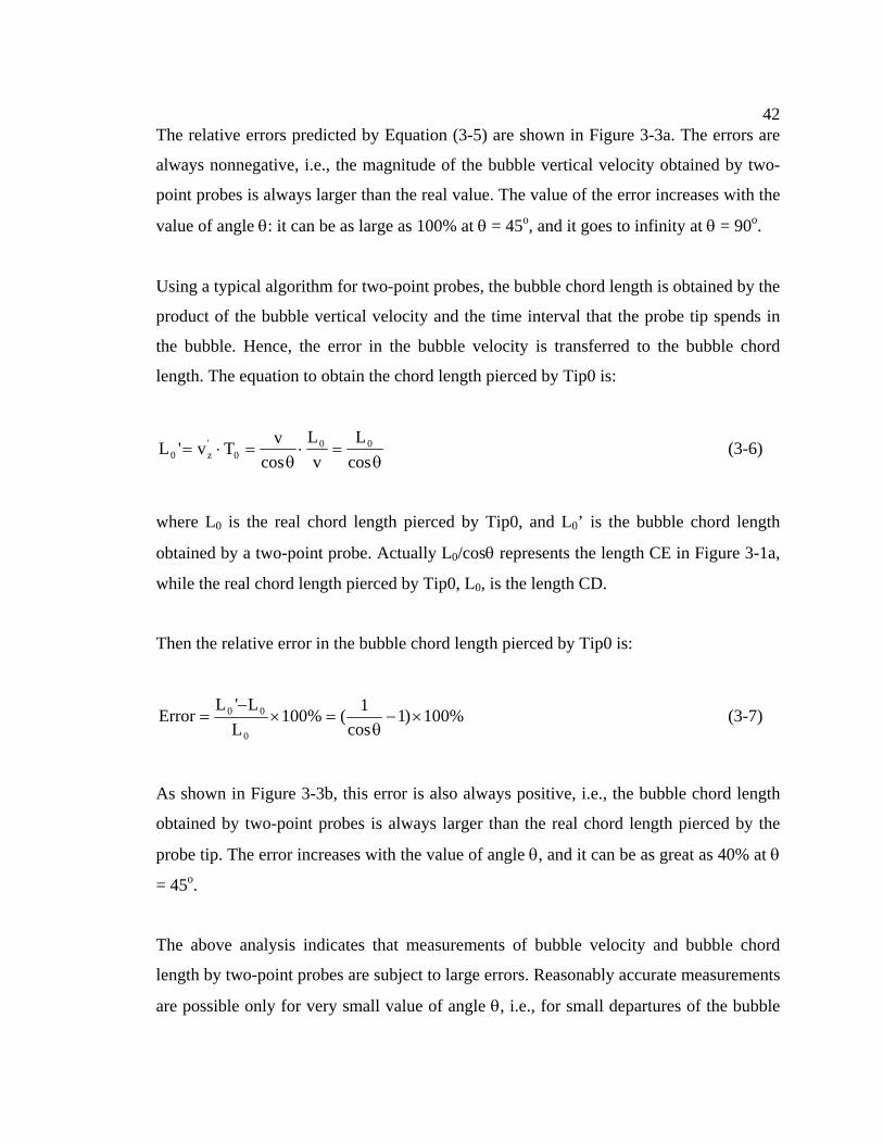
42 The relative errors predicted by Equation (3-5) are shown in Figure 3-3a. The errors are

always nonnegative, i.e., the magnitude of the bubble vertical velocity obtained by two-

point probes is always larger than the real value. The value of the error increases with the

value of angle θ: it can be as large as 100% at θ = 45o, and it goes to infinity at θ = 90o.

Using a typical algorithm for two-point probes, the bubble chord length is obtained by the

product of the bubble vertical velocity and the time interval that the probe tip spends in

the bubble. Hence, the error in the bubble velocity is transferred to the bubble chord

length. The equation to obtain the chord length pierced by Tip0 is:

θ=⋅

θ=⋅=

cosL

vL

cosvTv'L 00

0'z0 (3-6)

where L0 is the real chord length pierced by Tip0, and L0’ is the bubble chord length

obtained by a two-point probe. Actually L0/cosθ represents the length CE in Figure 3-1a,

while the real chord length pierced by Tip0, L0, is the length CD.

Then the relative error in the bubble chord length pierced by Tip0 is:

%100)1cos

1(%100L

L'LError

0

00 ×−θ

=×−

= (3-7)

As shown in Figure 3-3b, this error is also always positive, i.e., the bubble chord length

obtained by two-point probes is always larger than the real chord length pierced by the

probe tip. The error increases with the value of angle θ, and it can be as great as 40% at θ

= 45o.

The above analysis indicates that measurements of bubble velocity and bubble chord

length by two-point probes are subject to large errors. Reasonably accurate measurements

are possible only for very small value of angle θ, i.e., for small departures of the bubble

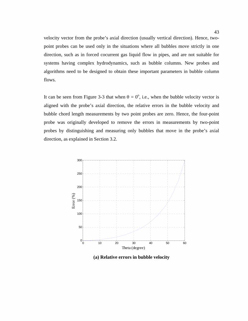
43 velocity vector from the probe’s axial direction (usually vertical direction). Hence, two-

point probes can be used only in the situations where all bubbles move strictly in one

direction, such as in forced cocurrent gas liquid flow in pipes, and are not suitable for

systems having complex hydrodynamics, such as bubble columns. New probes and

algorithms need to be designed to obtain these important parameters in bubble column

flows.

It can be seen from Figure 3-3 that when θ = 0o, i.e., when the bubble velocity vector is

aligned with the probe’s axial direction, the relative errors in the bubble velocity and

bubble chord length measurements by two point probes are zero. Hence, the four-point

probe was originally developed to remove the errors in measurements by two-point

probes by distinguishing and measuring only bubbles that move in the probe’s axial

direction, as explained in Section 3.2.

0 10 20 30 40 50 600

50

100

150

200

250

300

Theta (degree)

Erro

r (%

)

(a) Relative errors in bubble velocity

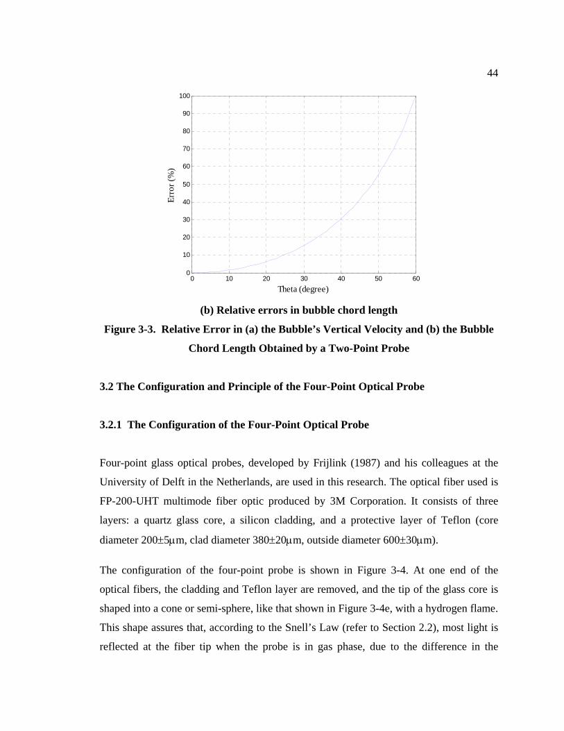
44

0 10 20 30 40 50 600

10

20

30

40

50

60

70

80

90

100

Theta (degree)

Erro

r (%

)

(b) Relative errors in bubble chord length

Figure 3-3. Relative Error in (a) the Bubble’s Vertical Velocity and (b) the Bubble

Chord Length Obtained by a Two-Point Probe

3.2 The Configuration and Principle of the Four-Point Optical Probe

3.2.1 The Configuration of the Four-Point Optical Probe

Four-point glass optical probes, developed by Frijlink (1987) and his colleagues at the

University of Delft in the Netherlands, are used in this research. The optical fiber used is

FP-200-UHT multimode fiber optic produced by 3M Corporation. It consists of three

layers: a quartz glass core, a silicon cladding, and a protective layer of Teflon (core

diameter 200±5µm, clad diameter 380±20µm, outside diameter 600±30µm). The configuration of the four-point probe is shown in Figure 3-4. At one end of the

optical fibers, the cladding and Teflon layer are removed, and the tip of the glass core is

shaped into a cone or semi-sphere, like that shown in Figure 3-4e, with a hydrogen flame.

This shape assures that, according to the Snell’s Law (refer to Section 2.2), most light is

reflected at the fiber tip when the probe is in gas phase, due to the difference in the

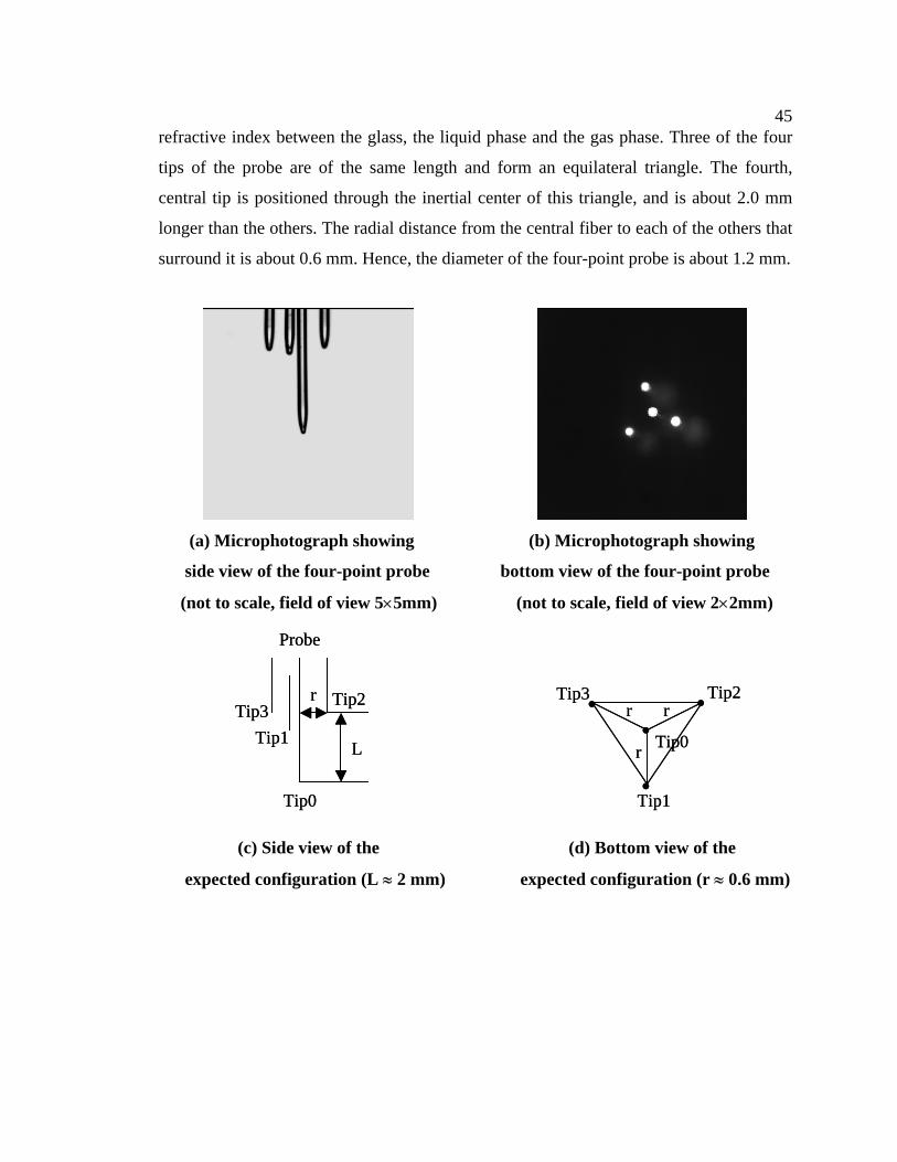
45 refractive index between the glass, the liquid phase and the gas phase. Three of the four

tips of the probe are of the same length and form an equilateral triangle. The fourth,

central tip is positioned through the inertial center of this triangle, and is about 2.0 mm

longer than the others. The radial distance from the central fiber to each of the others that

surround it is about 0.6 mm. Hence, the diameter of the four-point probe is about 1.2 mm.

(a) Microphotograph showing (b) Microphotograph showing

side view of the four-point probe bottom view of the four-point probe

(not to scale, field of view 5×5mm) (not to scale, field of view 2×2mm)

L

r

Probe

Tip0

Tip3Tip1

Tip2

L

r

Probe

Tip0

Tip3Tip1

Tip2

Tip1

Tip3 Tip2

•

••

•

Tip0

rr

r

Tip1

Tip3 Tip2

•

••

•

Tip0

rr

r

(c) Side view of the (d) Bottom view of the

expected configuration (L ≈ 2 mm) expected configuration (r ≈ 0.6 mm)

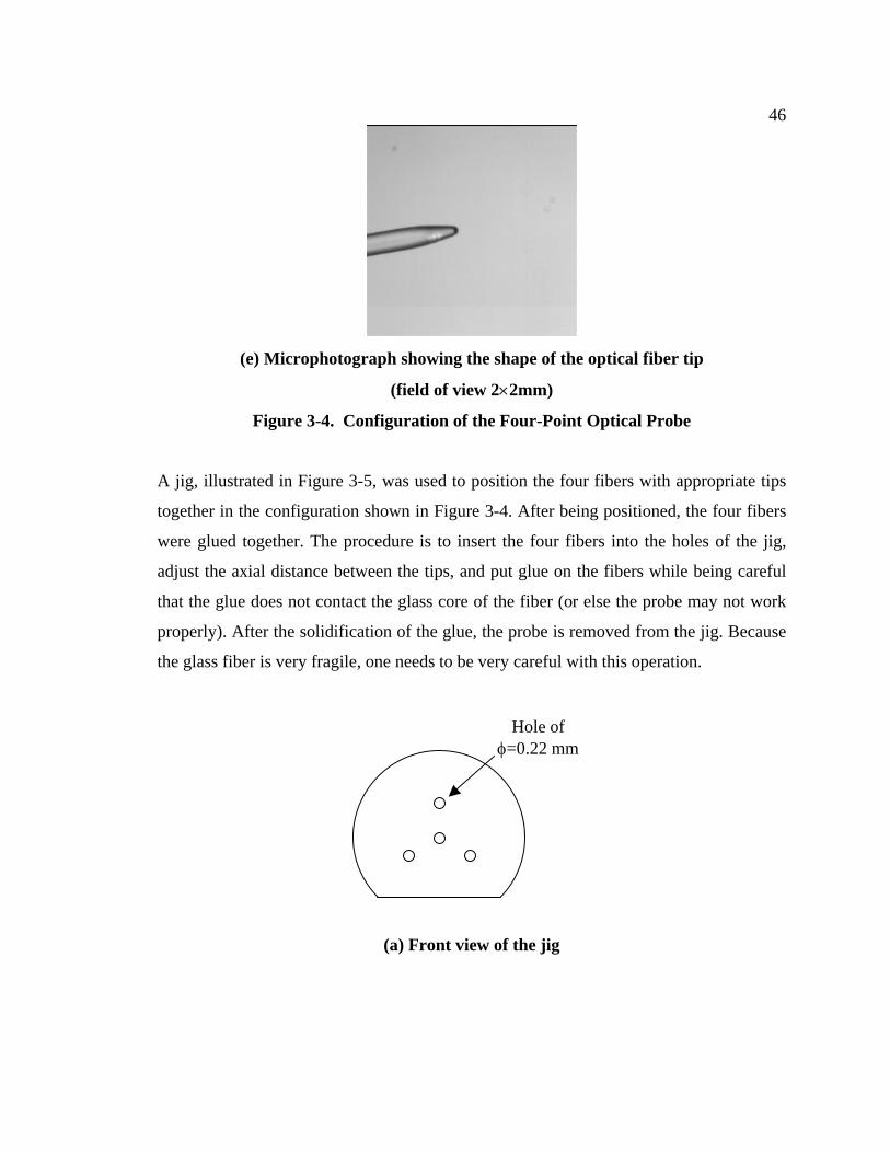
46

(e) Microphotograph showing the shape of the optical fiber tip

(field of view 2×2mm)

Figure 3-4. Configuration of the Four-Point Optical Probe

A jig, illustrated in Figure 3-5, was used to position the four fibers with appropriate tips

together in the configuration shown in Figure 3-4. After being positioned, the four fibers

were glued together. The procedure is to insert the four fibers into the holes of the jig,

adjust the axial distance between the tips, and put glue on the fibers while being careful

that the glue does not contact the glass core of the fiber (or else the probe may not work

properly). After the solidification of the glue, the probe is removed from the jig. Because

the glass fiber is very fragile, one needs to be very careful with this operation.

Hole of φ=0.22 mm

(a) Front view of the jig

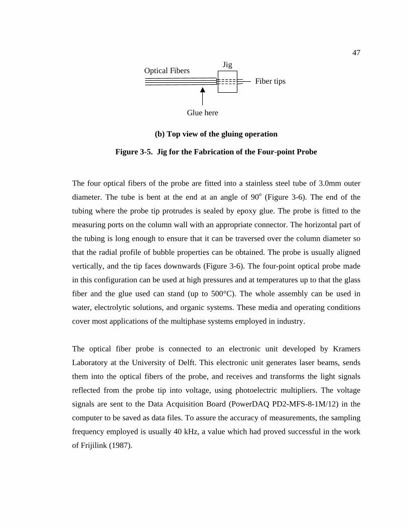
47 Jig

Optical Fibers

Glue here

Fiber tips

(b) Top view of the gluing operation

Figure 3-5. Jig for the Fabrication of the Four-point Probe

The four optical fibers of the probe are fitted into a stainless steel tube of 3.0mm outer

diameter. The tube is bent at the end at an angle of 90o (Figure 3-6). The end of the

tubing where the probe tip protrudes is sealed by epoxy glue. The probe is fitted to the

measuring ports on the column wall with an appropriate connector. The horizontal part of

the tubing is long enough to ensure that it can be traversed over the column diameter so

that the radial profile of bubble properties can be obtained. The probe is usually aligned

vertically, and the tip faces downwards (Figure 3-6). The four-point optical probe made

in this configuration can be used at high pressures and at temperatures up to that the glass

fiber and the glue used can stand (up to 500°C). The whole assembly can be used in

water, electrolytic solutions, and organic systems. These media and operating conditions

cover most applications of the multiphase systems employed in industry.

The optical fiber probe is connected to an electronic unit developed by Kramers

Laboratory at the University of Delft. This electronic unit generates laser beams, sends

them into the optical fibers of the probe, and receives and transforms the light signals

reflected from the probe tip into voltage, using photoelectric multipliers. The voltage

signals are sent to the Data Acquisition Board (PowerDAQ PD2-MFS-8-1M/12) in the

computer to be saved as data files. To assure the accuracy of measurements, the sampling

frequency employed is usually 40 kHz, a value which had proved successful in the work

of Frijilink (1987).

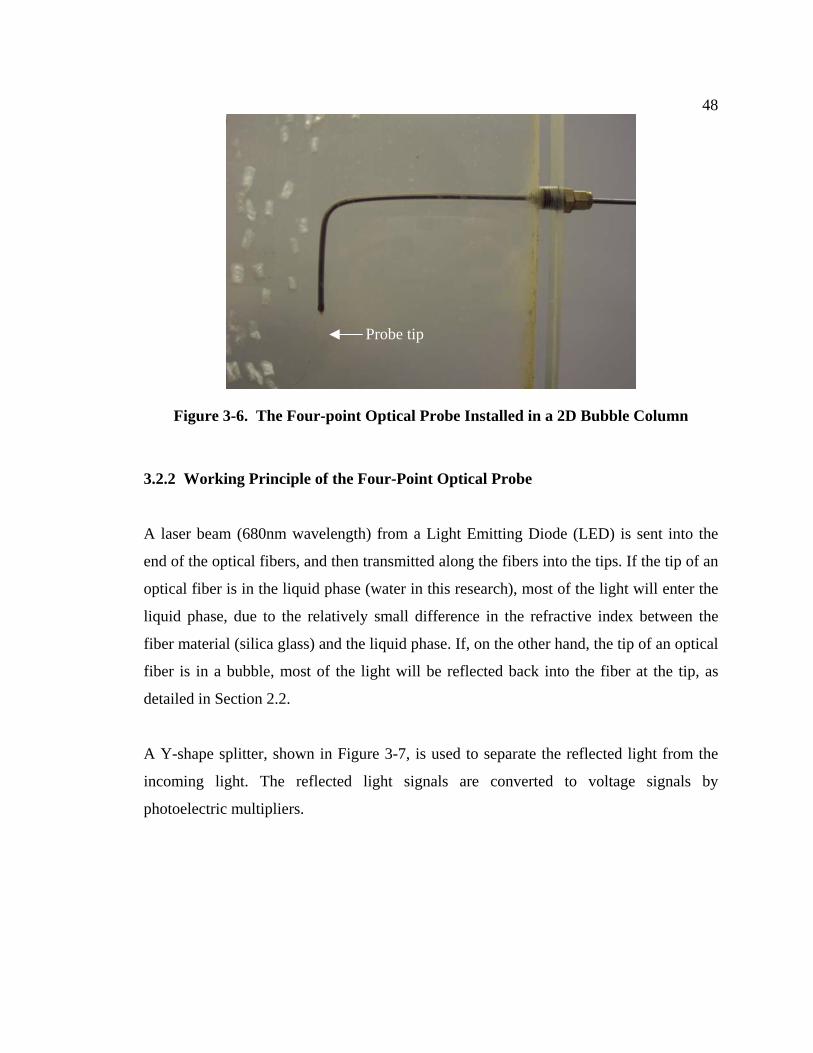
48

Probe tip

Figure 3-6. The Four-point Optical Probe Installed in a 2D Bubble Column

3.2.2 Working Principle of the Four-Point Optical Probe

A laser beam (680nm wavelength) from a Light Emitting Diode (LED) is sent into the

end of the optical fibers, and then transmitted along the fibers into the tips. If the tip of an

optical fiber is in the liquid phase (water in this research), most of the light will enter the

liquid phase, due to the relatively small difference in the refractive index between the

fiber material (silica glass) and the liquid phase. If, on the other hand, the tip of an optical

fiber is in a bubble, most of the light will be reflected back into the fiber at the tip, as

detailed in Section 2.2.

A Y-shape splitter, shown in Figure 3-7, is used to separate the reflected light from the

incoming light. The reflected light signals are converted to voltage signals by

photoelectric multipliers.

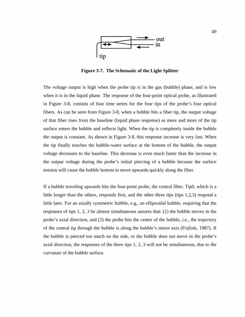
49

Figure 3-7. The Schematic of the Light Splitter

The voltage output is high when the probe tip is in the gas (bubble) phase, and is low

when it is in the liquid phase. The response of the four-point optical probe, as illustrated

in Figure 3-8, consists of four time series for the four tips of the probe’s four optical

fibers. As can be seen from Figure 3-8, when a bubble hits a fiber tip, the output voltage

of that fiber rises from the baseline (liquid phase response) as more and more of the tip

surface enters the bubble and reflects light. When the tip is completely inside the bubble

the output is constant. As shown in Figure 3-8, this response increase is very fast. When

the tip finally touches the bubble-water surface at the bottom of the bubble, the output

voltage decreases to the baseline. This decrease is even much faster than the increase in

the output voltage during the probe’s initial piercing of a bubble because the surface

tension will cause the bubble bottom to move upwards quickly along the fiber.

If a bubble traveling upwards hits the four-point probe, the central fiber, Tip0, which is a

little longer than the others, responds first, and the other three tips (tips 1,2,3) respond a

little later. For an axially symmetric bubble, e.g., an ellipsoidal bubble, requiring that the

responses of tips 1, 2, 3 be almost simultaneous assures that: (1) the bubble moves in the

probe’s axial direction, and (2) the probe hits the center of the bubble, i.e., the trajectory

of the central tip through the bubble is along the bubble’s minor axis (Frijlink, 1987). If

the bubble is pierced too much on the side, or the bubble does not move in the probe’s

axial direction, the responses of the three tips 1, 2, 3 will not be simultaneous, due to the

curvature of the bubble surface.

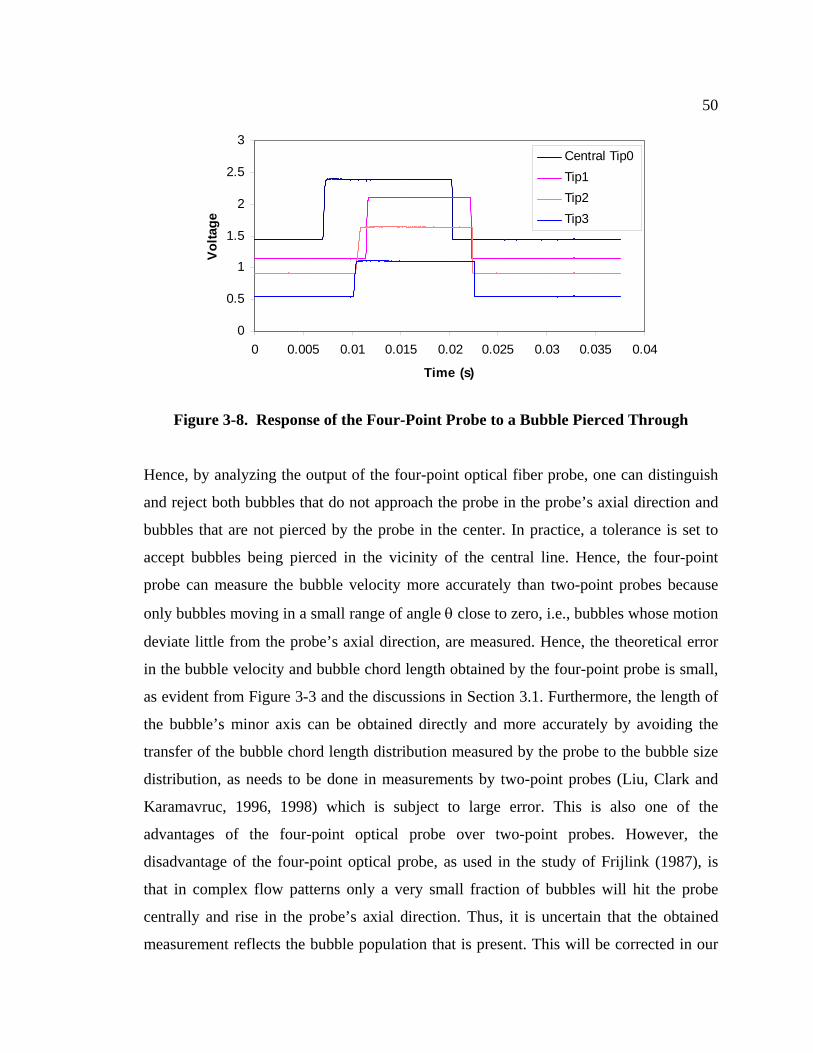
50

0

0.5

1

1.5

2

2.5

3

0 0.005 0.01 0.015 0.02 0.025 0.03 0.035 0.04

Time (s)

Volta

ge

Central Tip0 Tip1Tip2Tip3

Figure 3-8. Response of the Four-Point Probe to a Bubble Pierced Through

Hence, by analyzing the output of the four-point optical fiber probe, one can distinguish

and reject both bubbles that do not approach the probe in the probe’s axial direction and

bubbles that are not pierced by the probe in the center. In practice, a tolerance is set to

accept bubbles being pierced in the vicinity of the central line. Hence, the four-point

probe can measure the bubble velocity more accurately than two-point probes because

only bubbles moving in a small range of angle θ close to zero, i.e., bubbles whose motion

deviate little from the probe’s axial direction, are measured. Hence, the theoretical error

in the bubble velocity and bubble chord length obtained by the four-point probe is small,

as evident from Figure 3-3 and the discussions in Section 3.1. Furthermore, the length of

the bubble’s minor axis can be obtained directly and more accurately by avoiding the

transfer of the bubble chord length distribution measured by the probe to the bubble size

distribution, as needs to be done in measurements by two-point probes (Liu, Clark and

Karamavruc, 1996, 1998) which is subject to large error. This is also one of the

advantages of the four-point optical probe over two-point probes. However, the

disadvantage of the four-point optical probe, as used in the study of Frijlink (1987), is

that in complex flow patterns only a very small fraction of bubbles will hit the probe

centrally and rise in the probe’s axial direction. Thus, it is uncertain that the obtained

measurement reflects the bubble population that is present. This will be corrected in our

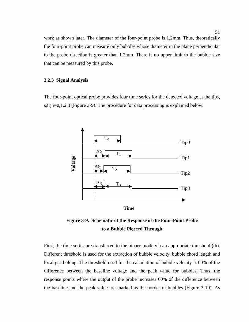
51 work as shown later. The diameter of the four-point probe is 1.2mm. Thus, theoretically

the four-point probe can measure only bubbles whose diameter in the plane perpendicular

to the probe direction is greater than 1.2mm. There is no upper limit to the bubble size

that can be measured by this probe.

3.2.3 Signal Analysis

The four-point optical probe provides four time series for the detected voltage at the tips,

si(t) i=0,1,2,3 (Figure 3-9). The procedure for data processing is explained below.

T0

T1

T2

T3

Tip0

Tip1

Tip2

Tip3

∆t1

∆t2

∆t3

Time

Vol

tage

Figure 3-9. Schematic of the Response of the Four-Point Probe

to a Bubble Pierced Through

First, the time series are transferred to the binary mode via an appropriate threshold (th).

Different threshold is used for the extraction of bubble velocity, bubble chord length and

local gas holdup. The threshold used for the calculation of bubble velocity is 60% of the

difference between the baseline voltage and the peak value for bubbles. Thus, the

response points where the output of the probe increases 60% of the difference between

the baseline and the peak value are marked as the border of bubbles (Figure 3-10). As

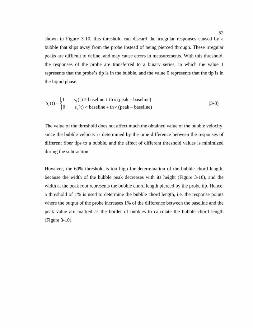
52 shown in Figure 3-10, this threshold can discard the irregular responses caused by a

bubble that slips away from the probe instead of being pierced through. These irregular

peaks are difficult to define, and may cause errors in measurements. With this threshold,

the responses of the probe are transferred to a binary series, in which the value 1

represents that the probe’s tip is in the bubble, and the value 0 represents that the tip is in

the liquid phase.

⎩⎨⎧

−×+<−×+≥

=)baselinepeak(thbaseline)t(s0)baselinepeak(thbaseline)t(s1

)t(bi

ii (3-8)

The value of the threshold does not affect much the obtained value of the bubble velocity,

since the bubble velocity is determined by the time difference between the responses of

different fiber tips to a bubble, and the effect of different threshold values is minimized

during the subtraction.

However, the 60% threshold is too high for determination of the bubble chord length,

because the width of the bubble peak decreases with its height (Figure 3-10), and the

width at the peak root represents the bubble chord length pierced by the probe tip. Hence,

a threshold of 1% is used to determine the bubble chord length, i.e. the response points

where the output of the probe increases 1% of the difference between the baseline and the

peak value are marked as the border of bubbles to calculate the bubble chord length

(Figure 3-10).

53

0.0

0.5

1.0

1.5

2.0

2.5

3.0

0 0.001 0.002 0.003 0.004 0.005 0.006 0.00

Time (s)

Vol

tage

(V)

060%

1%

discarded peak

Figure 3-10. A Sample of the Probe’s Responses

From the response of the probe’s central tip, the local gas holdup can be

N

t(b

TT

timetmeasuremenTotalbubblesintipcentrals'probethebyspentTime

N

1jj0

0g

∑∑ ==∆

==ε

where N is the total number of sample points in the response of the pr

When calculating the local gas holdup, all bubbles that hit the central tip

used, i.e., there is no rejection of any bubbles.

The threshold for the determination of gas holdup should not be too hig

cause bubbles that touch the tip rather than being pierced to be f

underestimating the gas holdup. Obviously, it cannot be too close to ze

unwanted noise would cause an overestimate of the gas holdup. B

threshold values, th, and calculating the gas holdup, εg, the relationship b

can be obtained, as shown in Figure 3-11 (as mentioned before, the unit

th, is the percentage of the difference between the baseline voltage and th

bubbles in Figure 3-11). Hence, a minimum threshold can be found, belo

Tip
1 Tip
2
Tip
3
Tip
7 0.008

obtained as:

) (3-9)

obe’s central tip.

of the probe are

h, as this would

iltered out, thus

ro either, as then

y using various

etween εg and th

of the threshold,

e peak value for

w which noise is

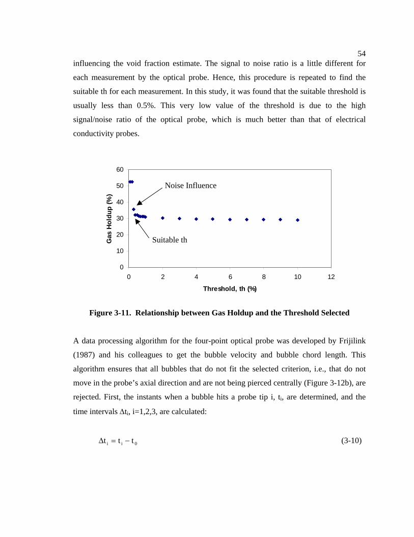
54 influencing the void fraction estimate. The signal to noise ratio is a little different for

each measurement by the optical probe. Hence, this procedure is repeated to find the

suitable th for each measurement. In this study, it was found that the suitable threshold is

usually less than 0.5%. This very low value of the threshold is due to the high

signal/noise ratio of the optical probe, which is much better than that of electrical

conductivity probes.

0

10

20

30

40

50

60

0 2 4 6 8 10 1

Threshold, th (%)

Gas

Hol

dup

(%)

2

Noise Influence

Suitable th

Figure 3-11. Relationship between Gas Holdup and the Threshold Selected

A data processing algorithm for the four-point optical probe was developed by Frijilink

(1987) and his colleagues to get the bubble velocity and bubble chord length. This

algorithm ensures that all bubbles that do not fit the selected criterion, i.e., that do not

move in the probe’s axial direction and are not being pierced centrally (Figure 3-12b), are

rejected. First, the instants when a bubble hits a probe tip i, ti, are determined, and the

time intervals ∆ti, i=1,2,3, are calculated:

0ii ttt −=∆ (3-10)

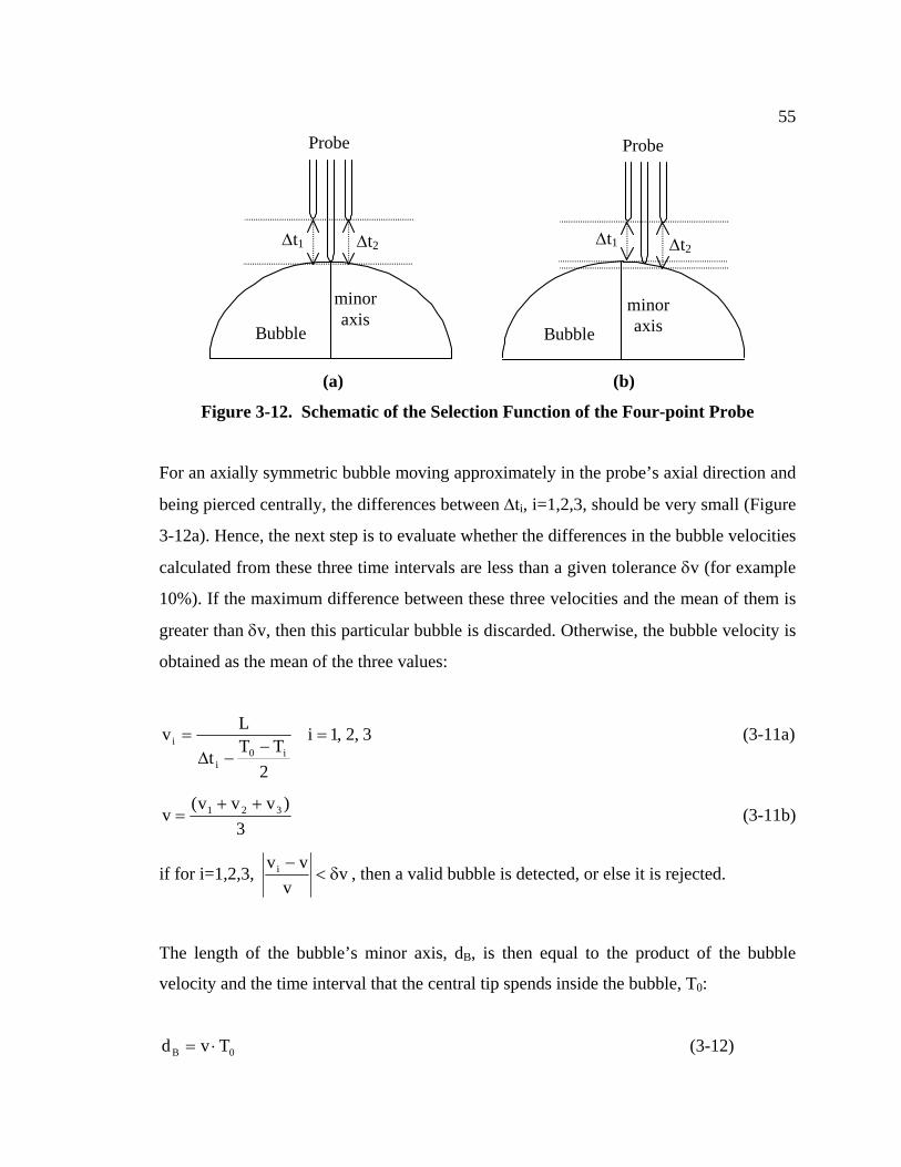
55

Bubble

Probe

minoraxis

∆t2∆t1

minor axis Bubble

Probe

∆t1 ∆t2

(a) (b)

Figure 3-12. Schematic of the Selection Function of the Four-point Probe

For an axially symmetric bubble moving approximately in the probe’s axial direction and

being pierced centrally, the differences between ∆ti, i=1,2,3, should be very small (Figure

3-12a). Hence, the next step is to evaluate whether the differences in the bubble velocities

calculated from these three time intervals are less than a given tolerance δv (for example

10%). If the maximum difference between these three velocities and the mean of them is

greater than δv, then this particular bubble is discarded. Otherwise, the bubble velocity is

obtained as the mean of the three values:

3,2,1i

2TT

t

Lvi0

i

i =−

−∆= (3-11a)

3)vvv(

v 321 ++= (3-11b)

if for i=1,2,3, vv

vvi δ<− , then a valid bubble is detected, or else it is rejected.

The length of the bubble’s minor axis, dB, is then equal to the product of the bubble

velocity and the time interval that the central tip spends inside the bubble, T0:

0B Tvd ⋅= (3-12)

563.2.4 Measurement Errors of the Four-Point Optical Probe (Old Algorithm) According to the data processing algorithm described in Section 3.2.3, the four-point

probe used in this work measures only bubbles that move almost in the probe’s axial

direction and are being pierced in the vicinity of the bubble’s central line by the central

tip of the probe. However, the movement of bubbles in bubble columns is rather

complicated. Actually bubbles do not move vertically and straight, but rather in a zigzag

or spiral pattern. Hence, if the probe is installed vertically in bubble columns, most

bubbles will move in directions that deviate from the probe’s axial direction, i.e., the

vertical direction.

Of course, it is not necessary that the probe be installed vertically. To reduce the

deviation of the bubble motion from the probe’s axial direction, it would be desirable to

place the probe in the direction of the motion of most bubbles, if such exists, at each

point in bubble columns. Unfortunately, it has been found that bubble motion in bubble

columns, including the movement direction, keeps changing with the liquid flow

direction all the time. There is no fixed preferred flow direction at most places in bubble

columns (Chen, Reese and Fan, 1994). As a result, it is practically impossible to align the

probe with the flow direction of bubbles, and many bubbles rise with a velocity direction

that deviates from the probe’s axial direction. Furthermore, the position where the probe

hits the bubble’s leading edge is random. Hence, the selection function of the probe is

difficult to apply efficiently. For example, in a 2-D column used, the bubble selection

with this probe (with tolerance δv=10%, see Equation 3-11) caused more than 99% of

bubbles that hit the probe to be discarded. This high selectivity causes difficulty in data

processing and interpretation. Therefore, to avoid a high discard ratio of bubbles during

the measurements, the effect of increasing the tolerance δv was studied so that bubbles

with movement that does deviate somewhat from the probe’s axial direction are also

accepted. To do this in a systematic manner, an error analysis was performed.

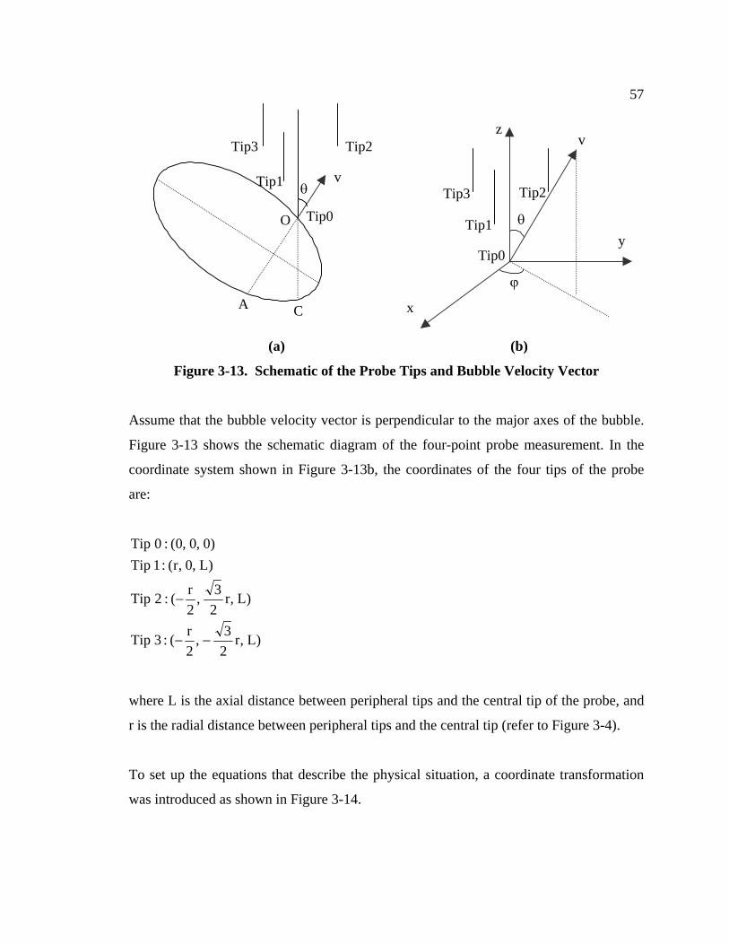
57

v

Tip2

A

θ

Tip3

Tip1

Tip0O

C

θ

ϕ

x

v z

y

Tip3

Tip1

Tip2

Tip0

(a) (b)

Figure 3-13. Schematic of the Probe Tips and Bubble Velocity Vector

Assume that the bubble velocity vector is perpendicular to the major axes of the bubble.

Figure 3-13 shows the schematic diagram of the four-point probe measurement. In the

coordinate system shown in Figure 3-13b, the coordinates of the four tips of the probe

are:

)L,r23,

2r(:3Tip

)L,r23,

2r(:2Tip

)L,0,r(:1Tip)0,0,0(:0Tip

−−

−

where L is the axial distance between peripheral tips and the central tip of the probe, and

r is the radial distance between peripheral tips and the central tip (refer to Figure 3-4).

To set up the equations that describe the physical situation, a coordinate transformation

was introduced as shown in Figure 3-14.

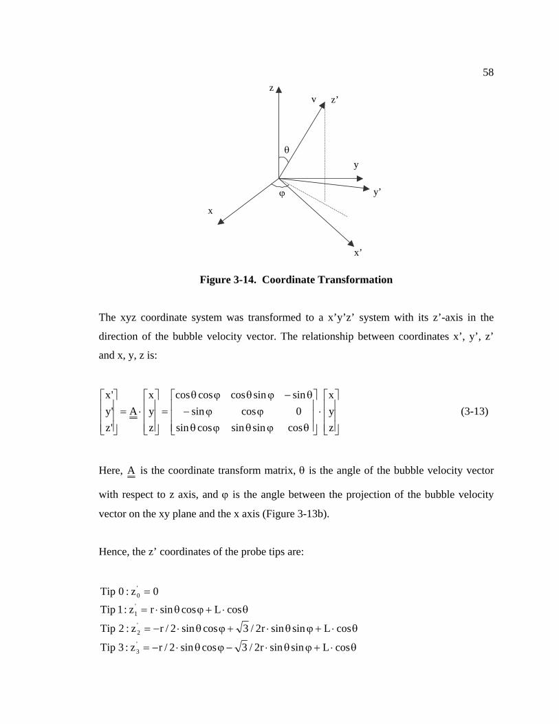
58

z

θ

ϕ

x

z’

y

y’

x’

v

Figure 3-14. Coordinate Transformation

The xyz coordinate system was transformed to a x’y’z’ system with its z’-axis in the

direction of the bubble velocity vector. The relationship between coordinates x’, y’, z’

and x, y, z is:

⎥⎥⎥

⎦

⎤

⎢⎢⎢

⎣

⎡⋅

⎥⎥⎥

⎦

⎤

⎢⎢⎢

⎣

⎡

θϕθϕθϕϕ−

θ−ϕθϕθ=

⎥⎥⎥

⎦

⎤

⎢⎢⎢

⎣

⎡⋅=

⎥⎥⎥

⎦

⎤

⎢⎢⎢

⎣

⎡

zyx

cossinsincossin0cossin

sinsincoscoscos

zyx

A'z'y'x

(3-13)

Here, A is the coordinate transform matrix, θ is the angle of the bubble velocity vector

with respect to z axis, and ϕ is the angle between the projection of the bubble velocity

vector on the xy plane and the x axis (Figure 3-13b).

Hence, the z’ coordinates of the probe tips are:

θ⋅+ϕθ⋅−ϕθ⋅−=

θ⋅+ϕθ⋅+ϕθ⋅−=

θ⋅+ϕθ⋅=

=

cosLsinsinr2/3cossin2/rz:3Tip

cosLsinsinr2/3cossin2/rz:2Tip

cosLcossinrz:1Tip

0z:0Tip

'3

'2

'1

'0

59 Notice that the zi’ coordinate value of Tip i, i=1,2,3, is the distance between Tip i and

Tip0 in the direction of the bubble velocity vector (Figure 3-13b). Hence, the time

intervals between the instant when a bubble hits the central tip, Tip0, and the instant

when it hits Tip i, i=1,2,3, are:

vcosLcossinr

2TT

t 101

θ⋅+ϕθ⋅=

−−∆ (3-14a)

vcosLsinsinr2/3cossin2/r

2TT

t 202

θ⋅+ϕθ⋅+ϕθ⋅−=

−−∆ (3-14b)

vcosLsinsinr2/3cossin2/r

2TT

t 303

θ⋅+ϕθ⋅−ϕθ⋅−=

−−∆ (3-14c)

where v is the magnitude of the bubble velocity vector.

Consequently, the magnitude of the component of the bubble velocity vector in the

probe’s axial direction obtained by the probe is:

)cosLsinsinr2/3cossin2/r

1cosLsinsinr2/3cossin2/r

1cosLcossinr

1(3Lv

2TT

t

L

2TT

t

L

2TT

t

L31'v

033

022

011

z

θ⋅+ϕθ⋅−ϕθ⋅−+

θ⋅+ϕθ⋅+ϕθ⋅−+

θ⋅+ϕθ⋅⋅⋅=

⎟⎟⎟⎟

⎠

⎞

⎜⎜⎜⎜

⎝

⎛

−−∆

+−

−∆+

−−∆

⋅=

(3-15)

As illustrated in Figure 3-13b, the real magnitude of the component of the bubble

velocity vector in the probe’s axial direction is:

θ⋅= cosvvz (3-16)

60 Hence, the relative error in the magnitude of the component of the bubble velocity vector

in the probe’s axial direction is:

%100cosv

cosv'v%100v

v'vError z

z

zz ×θ⋅θ⋅−

=×−

= (3-17)

Figure 3-15 shows the errors in measurements by the probe predicted by Equation (3-17).

The range of angle ϕ is selected as 0~60o. This range covers all the cases because of the

symmetry of the three peripheral tips of the probe. The range of angle θ is selected also

as 0~60o for the convenience of display. In this range of θ and ϕ, the relative error in the

magnitude of the bubble velocity component in the probe’s axial direction can be as large

as 400%. At θ values larger than 60o, the relative errors are even larger. It can be seen

from Figure 3-15 that the relative error is affected mainly by the value of angle θ. To

keep the relative error smaller than 25%, θ must be smaller than 25o.

Figures 3-16, 3-17, and 3-18 show the difference between the bubble velocity determined

by Tip i, vi i=1,2,3, and the mean of v1, v2, and v3. Assume the tolerance, δv, for the

bubble selection is set to be 10%, i.e., a bubble will be accepted only if the relative

differences between v1, v2, v3 and the mean, v, are all within ±10% (refer to Equation 3-

11). From Figures 3-16, 3-17, and 3-18, it can be seen that all bubbles with a velocity

vector that deviates from the probe’s axial direction within 20o will be accepted. The

relative error in the bubble velocity at θ=20o is about 15% according to Figure 3-15. If

the tolerance, δv, is set to be 20%, the tolerated range of θ by the probe measurement will

be larger than 30o. At θ=30o, the relative error in the bubble velocity is about 40%

according to Figure 3-15.

61

ϕ (degree)

(a) Surface diagra

ϕ (d

egre

e)

θ )

(b) Contour diagr

Figure 3-15. Relative Errors in Bubble Velocity M

of Bubble Motion from the Probe’s Axial Di

θ (degree)

m

(degree
am
easurements due to the Deviation

rection (r=0.6mm, L=1.5mm)

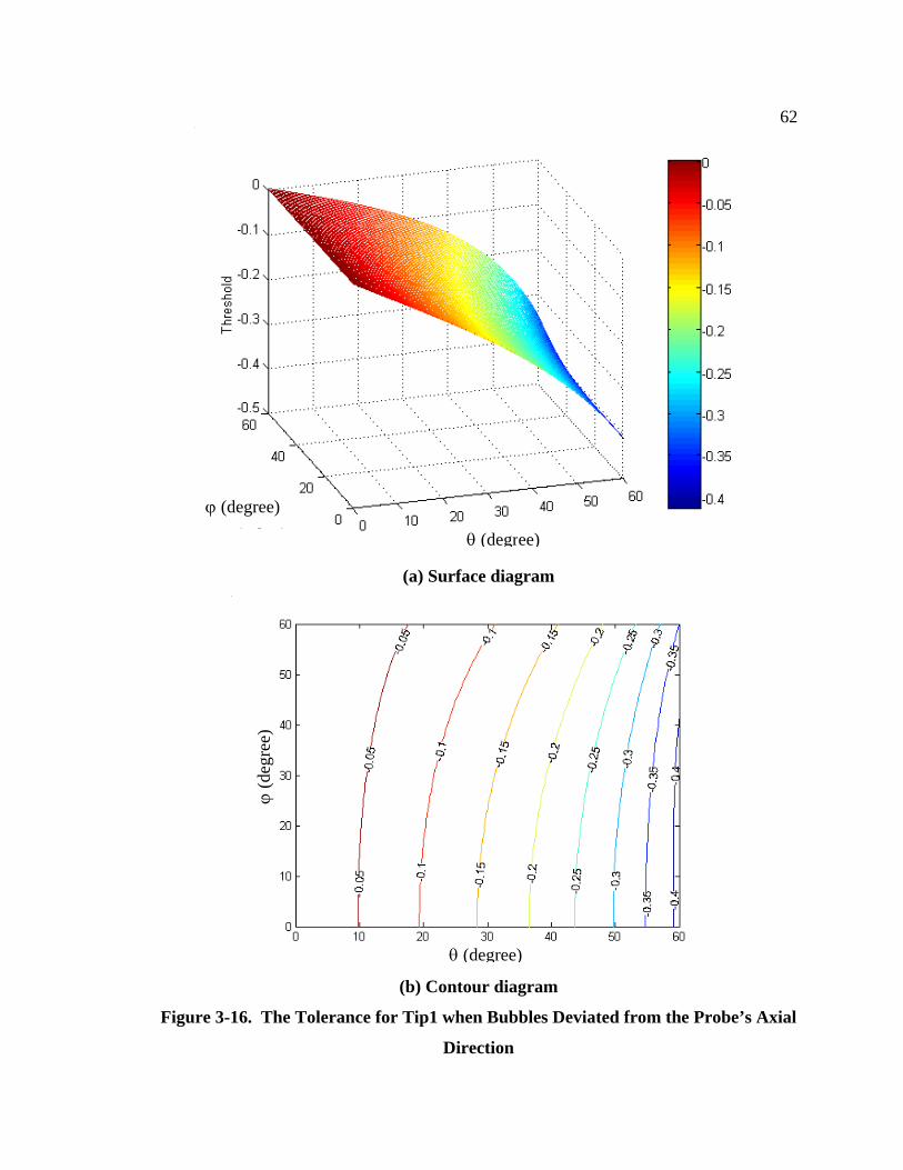
62

ϕ

Figure

(degree)

(a) Surfa

ϕ (d

egre

e)

θ (

(b) Conto

3-16. The Tolerance for Tip1 whe

Dir

θ (degree)
ce diagram
degree)

ur diagram

n Bubbles Deviated from the Probe’s Axial

ection

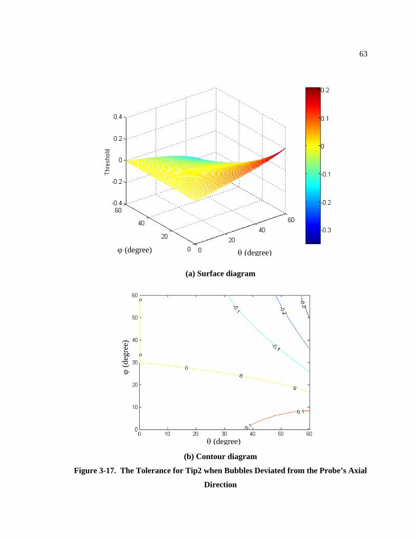
63

ϕ (degree) θ

(a) Surface diag

ϕ (d

egre

e)

θ

(b) Contour dia

Figure 3-17. The Tolerance for Tip2 when Bub

Direction

(degree)

ram

(degree)

gram

bles Deviated from the Probe’s Axial

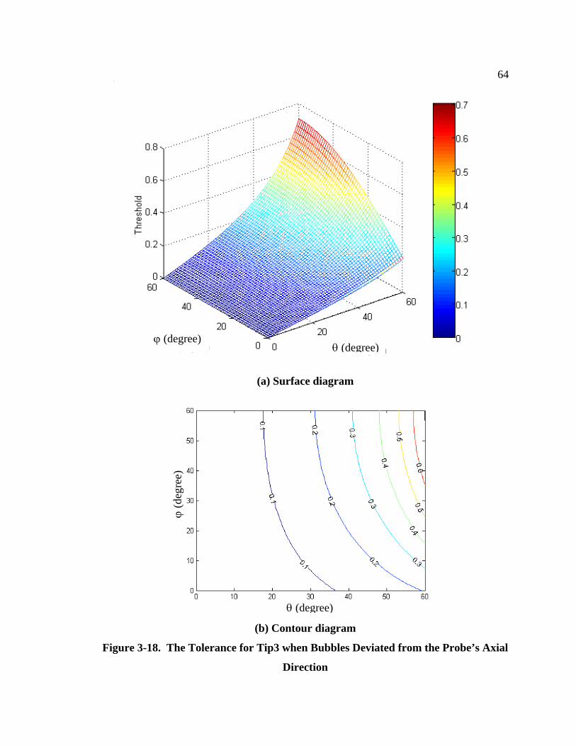
64

ϕ

Figure 3-18

(degree)
θ
(a) Surface diag

ϕ (d

egre

e)

θ

(b) Contour diag

. The Tolerance for Tip3 when Bubb

Direction

(degree)

ram

(degree)
ram
les Deviated from the Probe’s Axial

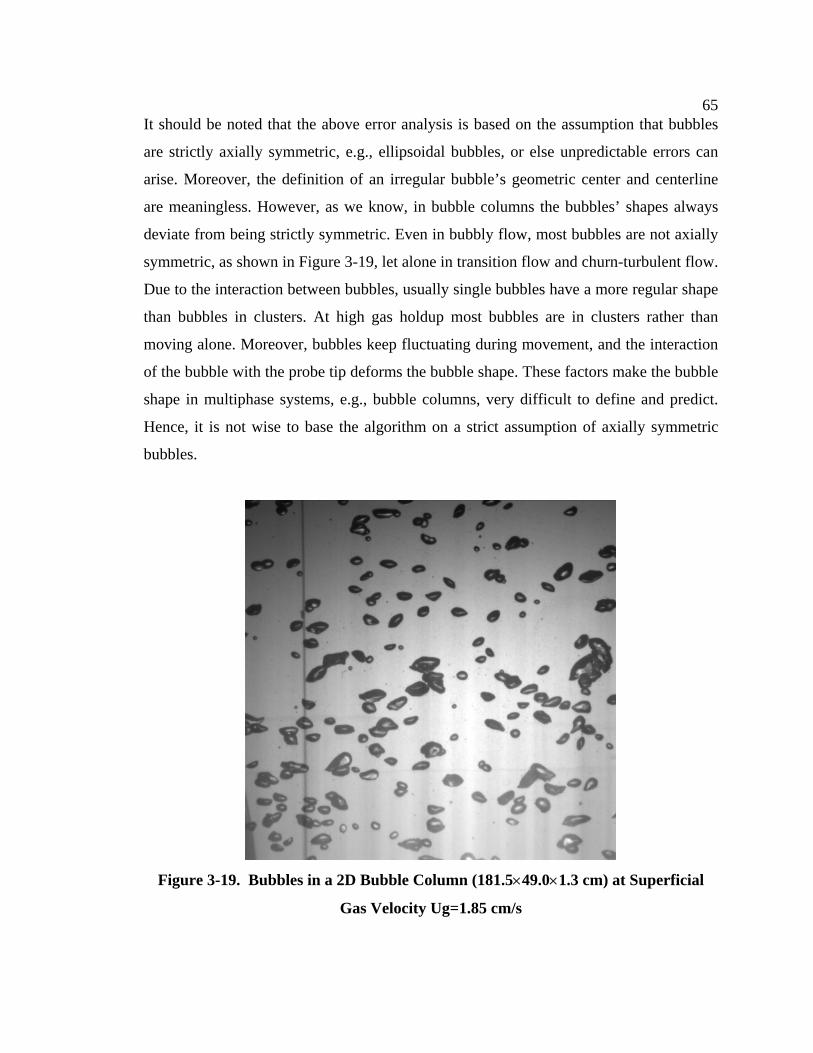
65 It should be noted that the above error analysis is based on the assumption that bubbles

are strictly axially symmetric, e.g., ellipsoidal bubbles, or else unpredictable errors can

arise. Moreover, the definition of an irregular bubble’s geometric center and centerline

are meaningless. However, as we know, in bubble columns the bubbles’ shapes always

deviate from being strictly symmetric. Even in bubbly flow, most bubbles are not axially

symmetric, as shown in Figure 3-19, let alone in transition flow and churn-turbulent flow.

Due to the interaction between bubbles, usually single bubbles have a more regular shape

than bubbles in clusters. At high gas holdup most bubbles are in clusters rather than

moving alone. Moreover, bubbles keep fluctuating during movement, and the interaction

of the bubble with the probe tip deforms the bubble shape. These factors make the bubble

shape in multiphase systems, e.g., bubble columns, very difficult to define and predict.

Hence, it is not wise to base the algorithm on a strict assumption of axially symmetric

bubbles.

Figure 3-19. Bubbles in a 2D Bubble Column (181.5×49.0×1.3 cm) at Superficial

Gas Velocity Ug=1.85 cm/s

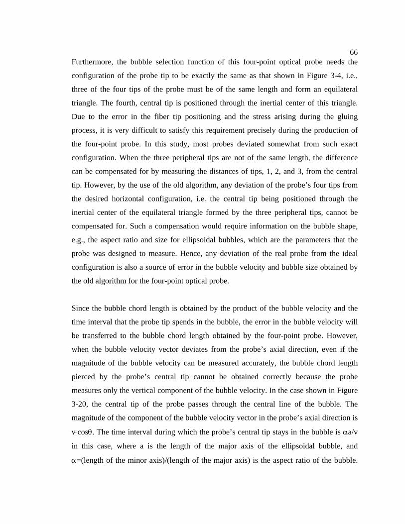
66Furthermore, the bubble selection function of this four-point optical probe needs the

configuration of the probe tip to be exactly the same as that shown in Figure 3-4, i.e.,

three of the four tips of the probe must be of the same length and form an equilateral

triangle. The fourth, central tip is positioned through the inertial center of this triangle.

Due to the error in the fiber tip positioning and the stress arising during the gluing

process, it is very difficult to satisfy this requirement precisely during the production of

the four-point probe. In this study, most probes deviated somewhat from such exact

configuration. When the three peripheral tips are not of the same length, the difference

can be compensated for by measuring the distances of tips, 1, 2, and 3, from the central

tip. However, by the use of the old algorithm, any deviation of the probe’s four tips from

the desired horizontal configuration, i.e. the central tip being positioned through the

inertial center of the equilateral triangle formed by the three peripheral tips, cannot be

compensated for. Such a compensation would require information on the bubble shape,

e.g., the aspect ratio and size for ellipsoidal bubbles, which are the parameters that the

probe was designed to measure. Hence, any deviation of the real probe from the ideal

configuration is also a source of error in the bubble velocity and bubble size obtained by

the old algorithm for the four-point optical probe.

Since the bubble chord length is obtained by the product of the bubble velocity and the

time interval that the probe tip spends in the bubble, the error in the bubble velocity will

be transferred to the bubble chord length obtained by the four-point probe. However,

when the bubble velocity vector deviates from the probe’s axial direction, even if the

magnitude of the bubble velocity can be measured accurately, the bubble chord length

pierced by the probe’s central tip cannot be obtained correctly because the probe

measures only the vertical component of the bubble velocity. In the case shown in Figure

3-20, the central tip of the probe passes through the central line of the bubble. The

magnitude of the component of the bubble velocity vector in the probe’s axial direction is

v⋅cosθ. The time interval during which the probe’s central tip stays in the bubble is αa/v

in this case, where a is the length of the major axis of the ellipsoidal bubble, and

α=(length of the minor axis)/(length of the major axis) is the aspect ratio of the bubble.

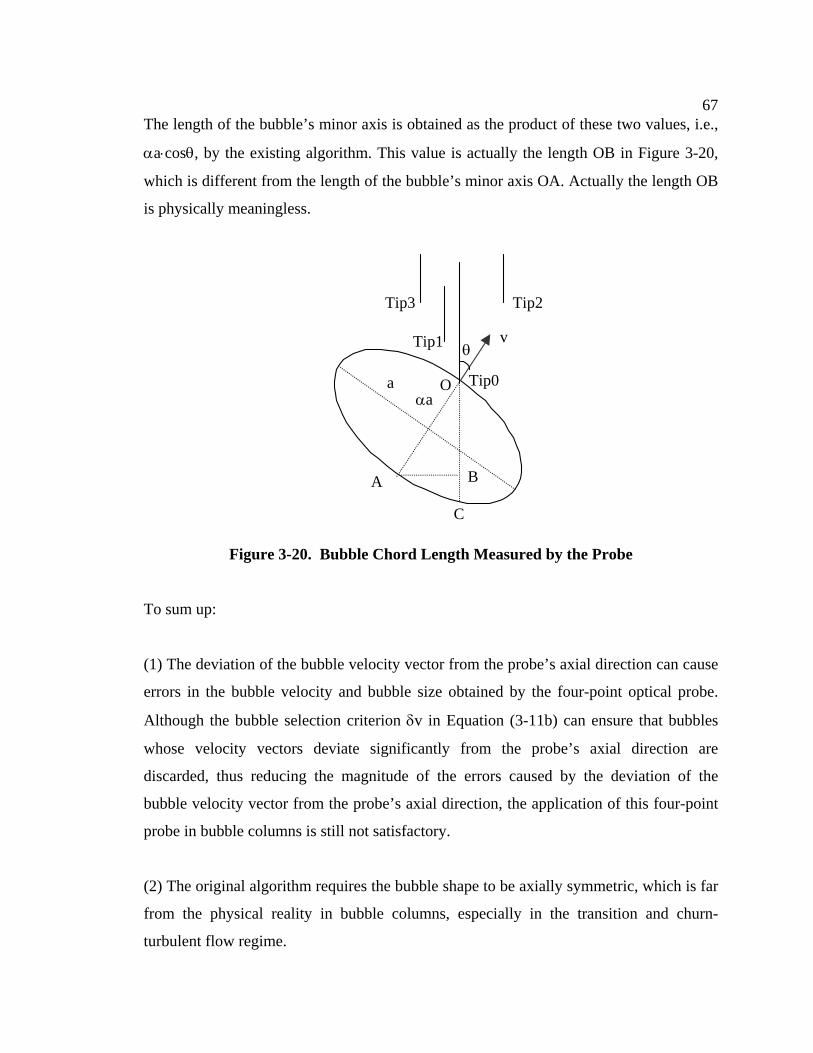
67 The length of the bubble’s minor axis is obtained as the product of these two values, i.e.,

αa⋅cosθ, by the existing algorithm. This value is actually the length OB in Figure 3-20,

which is different from the length of the bubble’s minor axis OA. Actually the length OB

is physically meaningless.

v

Tip2

B A

a αa

θ

Tip3

Tip1

Tip0O

C

Figure 3-20. Bubble Chord Length Measured by the Probe

To sum up:

(1) The deviation of the bubble velocity vector from the probe’s axial direction can cause

errors in the bubble velocity and bubble size obtained by the four-point optical probe.

Although the bubble selection criterion δv in Equation (3-11b) can ensure that bubbles

whose velocity vectors deviate significantly from the probe’s axial direction are

discarded, thus reducing the magnitude of the errors caused by the deviation of the

bubble velocity vector from the probe’s axial direction, the application of this four-point

probe in bubble columns is still not satisfactory.

(2) The original algorithm requires the bubble shape to be axially symmetric, which is far

from the physical reality in bubble columns, especially in the transition and churn-

turbulent flow regime.

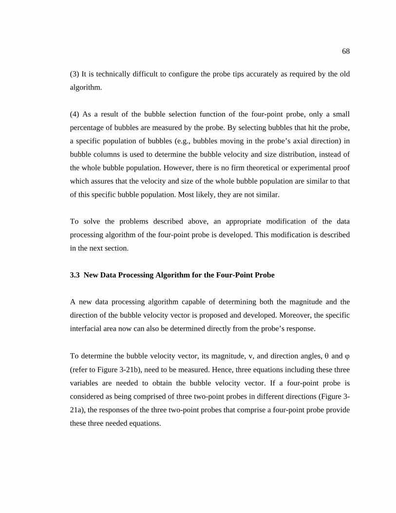
68

(3) It is technically difficult to configure the probe tips accurately as required by the old

algorithm.

(4) As a result of the bubble selection function of the four-point probe, only a small

percentage of bubbles are measured by the probe. By selecting bubbles that hit the probe,

a specific population of bubbles (e.g., bubbles moving in the probe’s axial direction) in

bubble columns is used to determine the bubble velocity and size distribution, instead of

the whole bubble population. However, there is no firm theoretical or experimental proof

which assures that the velocity and size of the whole bubble population are similar to that

of this specific bubble population. Most likely, they are not similar.

To solve the problems described above, an appropriate modification of the data

processing algorithm of the four-point probe is developed. This modification is described

in the next section.

3.3 New Data Processing Algorithm for the Four-Point Probe

A new data processing algorithm capable of determining both the magnitude and the

direction of the bubble velocity vector is proposed and developed. Moreover, the specific

interfacial area now can also be determined directly from the probe’s response.

To determine the bubble velocity vector, its magnitude, v, and direction angles, θ and ϕ

(refer to Figure 3-21b), need to be measured. Hence, three equations including these three

variables are needed to obtain the bubble velocity vector. If a four-point probe is

considered as being comprised of three two-point probes in different directions (Figure 3-

21a), the responses of the three two-point probes that comprise a four-point probe provide

these three needed equations.

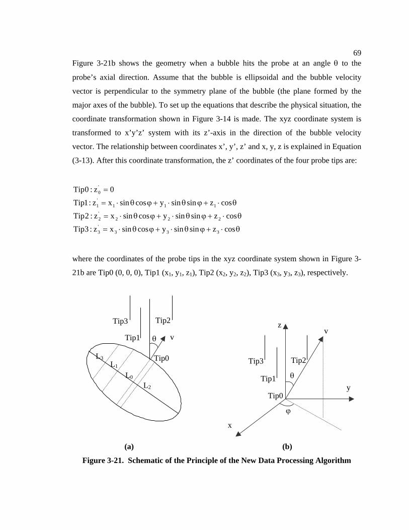
69

Figure 3-21b shows the geometry when a bubble hits the probe at an angle θ to the

probe’s axial direction. Assume that the bubble is ellipsoidal and the bubble velocity

vector is perpendicular to the symmetry plane of the bubble (the plane formed by the

major axes of the bubble). To set up the equations that describe the physical situation, the

coordinate transformation shown in Figure 3-14 is made. The xyz coordinate system is

transformed to x’y’z’ system with its z’-axis in the direction of the bubble velocity

vector. The relationship between coordinates x’, y’, z’ and x, y, z is explained in Equation

(3-13). After this coordinate transformation, the z’ coordinates of the four probe tips are:

θ⋅+ϕθ⋅+ϕθ⋅=



=

coszsinsinycossinxz:3Tipcoszsinsinycossinxz:2Tip

coszsinsinycossinxz:1Tip

0z:0Tip

333'3

222'2

111'1

'0

where the coordinates of the probe tips in the xyz coordinate system shown in Figure 3-

21b are Tip0 (0, 0, 0), Tip1 (x1, y1, z1), Tip2 (x2, y2, z2), Tip3 (x3, y3, z3), respectively.

v

Tip3

Tip1

Tip2

Tip0

θ

L3 L1

L2

L0

θ

ϕ

x

v z

y

Tip3

Tip1

Tip2

Tip0

(a) (b)

Figure 3-21. Schematic of the Principle of the New Data Processing Algorithm

70 Notice that the zi’ coordinate value of Tip i, i=1,2,3, is the distance between Tip i and

Tip0 in the direction of the bubble velocity vector (Figure 3-21). Accounting for the

curvature correction (explained in Section 3.1, Figure 3-2), the time intervals between the

instant when a bubble hits the central tip, Tip0, and when it hits Tip i, i=1,2,3 are:

vcoszsinsinycossinx

2TT

t 111101


−−∆ (3-18a)

vcoszsinsinycossinx

2TT

t 222202


−−∆ (3-18b)

vcoszsinsinycossinx

2TT

t 333303


−−∆ (3-18c)

This group of nonlinear equations for v, θ and ϕ does not yield analytical solutions. The

equations need to be solved numerically, e.g., with a Newton-Raphson algorithm. As a

result, the velocity magnitude, v, and the direction angles, θ and ϕ, of the bubble velocity

vector are obtained. Based on these values, the bubble chord length pierced by Tip i, Li,

i=0, 1, 2, 3, can be obtained by:

ii TvL ⋅= (3-19)

The chord length distribution obtained by the probe then needs to be transformed to the

‘equivalent’ bubble diameter distribution. Liu et al. (1996, 1998) developed an algorithm

to transform the bubble chord length distribution obtained by a two-point probe to the

bubble size distribution when bubbles are spherical, ellipsoidal or truncated ellipsoidal.

To use this algorithm, the aspect ratio of the bubbles, α=(length of minor axis)/(length of

major axis), in the system needs to be known or assumed in advance. Usually α is

empirically set as a single value. However, in bubble columns α is not a single value but

a distribution, and there is no way to estimate the mean aspect ratio in advance. Hence,

this oversimplification may cause large errors in the transformation of bubble chord

length distribution to bubble size distribution. Besides, Liu’s algorithm is very sensitive

71 to errors in the bubble chord length distribution, i.e., small changes in the bubble chord

length distribution obtained may cause significant changes in the bubble size distribution

calculated. Hence, Liu’s algorithm for the transfer of the bubble chord length distribution

to the bubble diameter distribution is not really applicable to bubble columns. So far,

there is no other reported algorithm for the transformation of the bubble chord length

distribution to the bubble size distribution.

As to the four-point optical probe, after the bubble chord lengths are obtained,

theoretically the bubble size can be calculated based on the assumption of the bubble

shape. The algorithm is explained below, and is valid not only for ellipsoidal bubbles but

also for any bubble whose shape can be expressed mathematically. Assume that the

bubble is ellipsoidal, with the minor axis as the revolution axis, as shown in Figure 3-22a.

The equation of the ellipsoid in Figure 3-22b is , where α is the aspect

ratio and c is a half of the length of the major axis. From Figure 3-22b it can be seen that

in the above equation x is the distance between the chord pierced by the probe’s tip to the

bubble’s center O, i.e., the length OC, and y equals half of the chord length, L

22222 cxy α=α+

i/2.

The four bubble chord lengths obtained by the four tips of the probe give four equations:

[ 222c0

2c0

22

0 c)y'y()x'x(2

Lα=−+−α+⎟

⎠⎞

⎜⎝⎛ ] (3-20a)

[ 222c1

2c1

22

1 c)y'y()x'x(2

Lα=−+−α+⎟

⎠⎞

⎜⎝⎛ ] (3-20b)

[ 222c2

2c2

22

2 c)y'y()x'x(2

Lα=−+−α+⎟

⎠⎞

⎜⎝⎛ ] (3-20c)

[ 222c3

2c3

22

3 c)y'y()x'x(2

Lα=−+−α+⎟

⎠⎞

⎜⎝⎛ ] (3-20d)

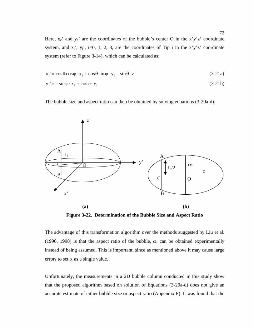
72 Here, xc’ and yc’ are the coordinates of the bubble’s center O in the x’y’z’ coordinate

system, and xi’, yi’, i=0, 1, 2, 3, are the coordinates of Tip i in the x’y’z’ coordinate

system (refer to Figure 3-14), which can be calculated as:

iiii zsinysincosxcoscos'x ⋅θ−⋅ϕθ+⋅ϕθ= (3-21a)

iii ycosxsin'y ⋅ϕ+⋅ϕ−= (3-21b)

The bubble size and aspect ratio can then be obtained by solving equations (3-20a-d).

z’

y’

x’

Li

O

B

A

C

A

B

C O

Li/2 c αc

(a) (b)

Figure 3-22. Determination of the Bubble Size and Aspect Ratio

The advantage of this transformation algorithm over the methods suggested by Liu et al.

(1996, 1998) is that the aspect ratio of the bubble, α, can be obtained experimentally

instead of being assumed. This is important, since as mentioned above it may cause large

errors to set α as a single value.

Unfortunately, the measurements in a 2D bubble column conducted in this study show

that the proposed algorithm based on solution of Equations (3-20a-d) does not give an

accurate estimate of either bubble size or aspect ratio (Appendix F). It was found that the

73 algorithm always underestimates the bubble aspect ratio, and is very sensitive to changes

of the bubble chord lengths obtained by the probe, i.e., small changes in the bubble chord

lengths may cause large variations in the calculated bubble size and aspect ratio. In 3D

bubble columns, the shape of bubbles deviates much more from ellipsoidal than in the 2D

bubble column at very low gas holdup. Hence, it is expected that the error in the bubble

sizes and aspect ratios obtained by the four-point probe will be even larger in 3D bubble

columns. As a result, this method is not recommended to investigate the bubble size and

shape in bubble columns. Instead, the bubble chord length distributions obtained by the

four-point probe were used to gain information on the bubble size distribution in bubble

columns, e.g., to determine whether the bubble size distribution in churn-turbulent flow is

bimodal or single modal.

One of the assumptions for all of the above analysis is that the bubble velocity vector

aligns with the bubble orientation. Usually this is true, due to the balance of the forces on

bubbles and the shape flexibility of gas bubbles. However, when the bubble’s motion

direction changes significantly as sometimes in churn-turbulent flow, it was observed that

the bubble velocity vector might deviate from the normal vector of the bubble’s

symmetry plane by an angle, φ, as shown in Figure 3-23a. This deviation may cause

errors in the bubble velocity vector and bubble chord length obtained by the four-point

optical probe.

From Figure 3-23c, it can be derived that the time intervals between the instant when a

bubble hits the central Tip0 and when it hits Tipi, i=1,2,3 are:

φ⋅θ⋅+ϕθ⋅+ϕθ⋅

=φ

=−

−∆cosv

coszsinsinycossinxvcos/z

2TT

t 111'110

1 (3-22a)


=φ

=−

−∆cosv


2TT

t 222'220

2 (3-22b)


=φ

=−

−∆cosv


2TT

t 333'330

3 (3-22c)

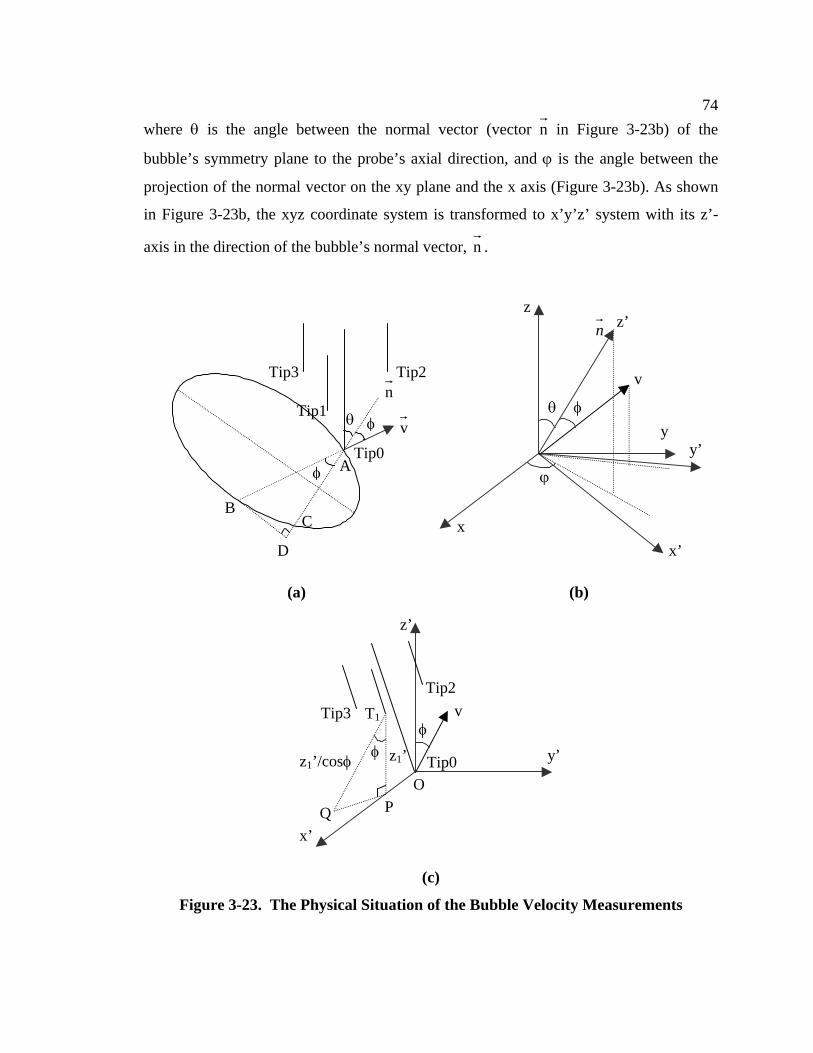
74

where θ is the angle between the normal vector (vector n in Figure 3-23b) of the

bubble’s symmetry plane to the probe’s axial direction, and ϕ is the angle between the

projection of the normal vector on the xy plane and the x axis (Figure 3-23b). As shown

in Figure 3-23b, the xyz coordinate system is transformed to x’y’z’ system with its z’-

axis in the direction of the bubble’s normal vector, n .

v

Tip2

B

D

θ

Tip3

Tip1

Tip0A

φ

n

φ

C

z

θ

ϕ

x

z’

y y’

x’

n

v

φ

(a) (b)

O

x’

v

z’

y’

Tip3 T1

Tip2

Tip0

φ φ z1’/cosφ

Q P

z1’

(c)

Figure 3-23. The Physical Situation of the Bubble Velocity Measurements

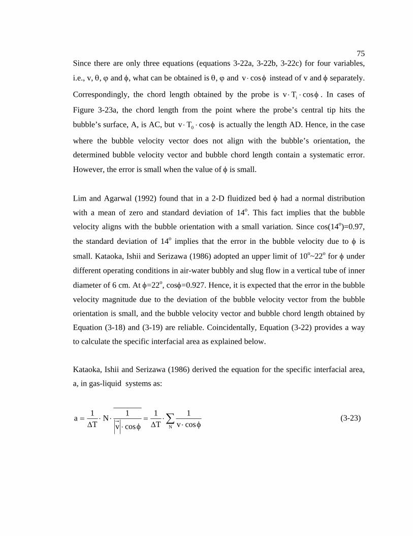
75 Since there are only three equations (equations 3-22a, 3-22b, 3-22c) for four variables,

i.e., v, θ, ϕ and φ, what can be obtained is θ, ϕ and φ⋅ cosv instead of v and φ separately.

Correspondingly, the chord length obtained by the probe is φ⋅⋅ cosTv i . In cases of

Figure 3-23a, the chord length from the point where the probe’s central tip hits the

bubble’s surface, A, is AC, but φ⋅⋅ cosTv 0 is actually the length AD. Hence, in the case

where the bubble velocity vector does not align with the bubble’s orientation, the

determined bubble velocity vector and bubble chord length contain a systematic error.

However, the error is small when the value of φ is small.

Lim and Agarwal (1992) found that in a 2-D fluidized bed φ had a normal distribution

with a mean of zero and standard deviation of 14o. This fact implies that the bubble

velocity aligns with the bubble orientation with a small variation. Since cos(14o)=0.97,

the standard deviation of 14o implies that the error in the bubble velocity due to φ is

small. Kataoka, Ishii and Serizawa (1986) adopted an upper limit of 10o~22o for φ under

different operating conditions in air-water bubbly and slug flow in a vertical tube of inner

diameter of 6 cm. At φ=22o, cosφ=0.927. Hence, it is expected that the error in the bubble

velocity magnitude due to the deviation of the bubble velocity vector from the bubble

orientation is small, and the bubble velocity vector and bubble chord length obtained by

Equation (3-18) and (3-19) are reliable. Coincidentally, Equation (3-22) provides a way

to calculate the specific interfacial area as explained below.

Kataoka, Ishii and Serizawa (1986) derived the equation for the specific interfacial area,

a, in gas-liquid systems as:

∑ φ⋅⋅

∆=

φ⋅⋅⋅

∆=

N cosv1

T1

cosv

1NT

1a (3-23)

76 where N is the total number of the gas-liquid interfaces passing by the probe during the

measurement time ∆T, and φ is the angle between the velocity vector and the normal

vector of the gas-liquid interface (e.g., the bubble’s surface).

Based on Equation (3-23), the four-point optical probe can be employed to obtain the

specific interfacial area. The physical situation is shown in Figure 3-24. Assume that the

gas-liquid interface (bubble surface) section between the three tips, Tip1, Tip2 and Tip3,

of the probe (Figure 3-24a) is flat. Considering the small size of the probe tip (1.2 mm in

diameter), this is a reasonable assumption except when the probe hits a gas-liquid

interface with large curvature, e.g., bubbles of very small horizontal dimension.

Note that the bubble leading edges and trailing edges both should be accounted for in the

specific interfacial area, and the curvature correction mentioned above (Figure 3-2) is

unnecessary (that curvature correction is valid only for measurements of the velocity of

the bubble’s centroid instead of the velocity of the bubble surface section).

ln

Probe

v

v

Tip2

θ

Tip3

Tip1

Tip0O

φln

Bubble

lnA

(a) (b)

Figure 3-24. The Physical Situation of Measurements of the Specific Interfacial

Area by the Four-Point Probe

77 The equations to determine the velocity of the bubble surface section are:


=φ

=∆cosv


t 111'1

1 (3-24a)


=φ

=∆cosv


t 222'2

2 (3-24b)


=φ

=∆cosv


t 333'3

3 (3-24c)

By solving these three equations numerically, the value of φ⋅ cosv can be obtained,

which can then be used to obtain the specific interfacial area from Equation (3-23).

However, if a bubble hits the central tip of the probe but misses some of the three

peripheral tips, then the bubble surface velocity vector cannot be obtained, due to the

insufficient number of equations, although this bubble contributes to the specific

interfacial area at the probe’s central tip. To account for the contribution of these

“missed” bubbles, the average value of φ⋅ cosv of bubbles that pass all the four tips of

the probe will be assigned to these “missed” bubbles. Hence, the equation for the

calculation of specific interfacial area is:

∑∑ φ⋅⋅

∆≅

φ⋅⋅

∆=

measuredNmeasuredN cosv1

NN

T1

cosv1

T1a (3-25a)

missedmeasured NNN += (3-25b)

Equations (3-24) and (3-25) do not need assumptions about bubble shape. Thus, errors

due to the inaccuracy in the bubble shape assumption can be avoided, leading to a robust

algorithm.

In churn-turbulent flow, the shape of many bubbles is highly irregular, and cannot be

described as any simple geometric shape, especially for large bubbles. Nevertheless, the

Sauter mean bubble diameter (the volume-surface mean diameter of bubbles) as shown in

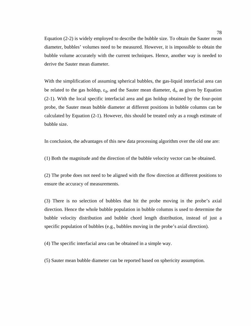
78Equation (2-2) is widely employed to describe the bubble size. To obtain the Sauter mean

diameter, bubbles’ volumes need to be measured. However, it is impossible to obtain the

bubble volume accurately with the current techniques. Hence, another way is needed to

derive the Sauter mean diameter.

With the simplification of assuming spherical bubbles, the gas-liquid interfacial area can

be related to the gas holdup, εg, and the Sauter mean diameter, ds, as given by Equation

(2-1). With the local specific interfacial area and gas holdup obtained by the four-point

probe, the Sauter mean bubble diameter at different positions in bubble columns can be

calculated by Equation (2-1). However, this should be treated only as a rough estimate of

bubble size.

In conclusion, the advantages of this new data processing algorithm over the old one are:

(1) Both the magnitude and the direction of the bubble velocity vector can be obtained.

(2) The probe does not need to be aligned with the flow direction at different positions to

ensure the accuracy of measurements.

(3) There is no selection of bubbles that hit the probe moving in the probe’s axial

direction. Hence the whole bubble population in bubble columns is used to determine the

bubble velocity distribution and bubble chord length distribution, instead of just a

specific population of bubbles (e.g., bubbles moving in the probe’s axial direction).

(4) The specific interfacial area can be obtained in a simple way.

(5) Sauter mean bubble diameter can be reported based on sphericity assumption.

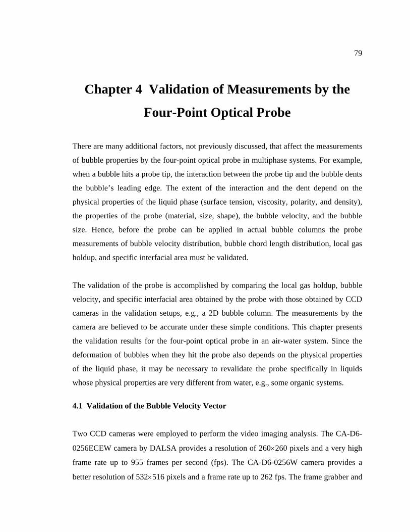
79

Chapter 4 Validation of Measurements by the


There are many additional factors, not previously discussed, that affect the measurements

of bubble properties by the four-point optical probe in multiphase systems. For example,

when a bubble hits a probe tip, the interaction between the probe tip and the bubble dents

the bubble’s leading edge. The extent of the interaction and the dent depend on the

physical properties of the liquid phase (surface tension, viscosity, polarity, and density),

the properties of the probe (material, size, shape), the bubble velocity, and the bubble

size. Hence, before the probe can be applied in actual bubble columns the probe

measurements of bubble velocity distribution, bubble chord length distribution, local gas

holdup, and specific interfacial area must be validated.

The validation of the probe is accomplished by comparing the local gas holdup, bubble

velocity, and specific interfacial area obtained by the probe with those obtained by CCD

cameras in the validation setups, e.g., a 2D bubble column. The measurements by the

camera are believed to be accurate under these simple conditions. This chapter presents

the validation results for the four-point optical probe in an air-water system. Since the

deformation of bubbles when they hit the probe also depends on the physical properties

of the liquid phase, it may be necessary to revalidate the probe specifically in liquids

whose physical properties are very different from water, e.g., some organic systems.

4.1 Validation of the Bubble Velocity Vector

Two CCD cameras were employed to perform the video imaging analysis. The CA-D6-

0256ECEW camera by DALSA provides a resolution of 260×260 pixels and a very high

frame rate up to 955 frames per second (fps). The CA-D6-0256W camera provides a

better resolution of 532×516 pixels and a frame rate up to 262 fps. The frame grabber and

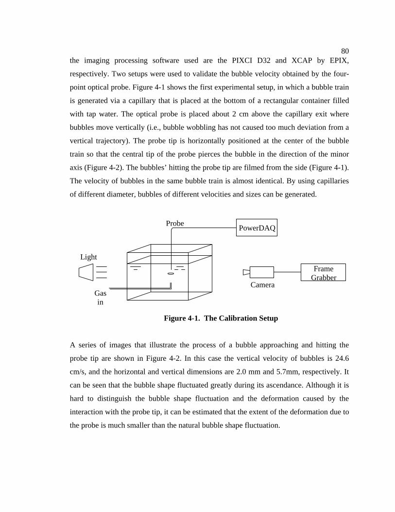
80the imaging processing software used are the PIXCI D32 and XCAP by EPIX,

respectively. Two setups were used to validate the bubble velocity obtained by the four-

point optical probe. Figure 4-1 shows the first experimental setup, in which a bubble train

is generated via a capillary that is placed at the bottom of a rectangular container filled

with tap water. The optical probe is placed about 2 cm above the capillary exit where

bubbles move vertically (i.e., bubble wobbling has not caused too much deviation from a

vertical trajectory). The probe tip is horizontally positioned at the center of the bubble

train so that the central tip of the probe pierces the bubble in the direction of the minor

axis (Figure 4-2). The bubbles’ hitting the probe tip are filmed from the side (Figure 4-1).

The velocity of bubbles in the same bubble train is almost identical. By using capillaries

of different diameter, bubbles of different velocities and sizes can be generated.

PowerDAQ

Frame Grabber

Light

Gas in

Probe

Camera

Figure 4-1. The Calibration Setup

A series of images that illustrate the process of a bubble approaching and hitting the

probe tip are shown in Figure 4-2. In this case the vertical velocity of bubbles is 24.6

cm/s, and the horizontal and vertical dimensions are 2.0 mm and 5.7mm, respectively. It

can be seen that the bubble shape fluctuated greatly during its ascendance. Although it is

hard to distinguish the bubble shape fluctuation and the deformation caused by the

interaction with the probe tip, it can be estimated that the extent of the deformation due to

the probe is much smaller than the natural bubble shape fluctuation.

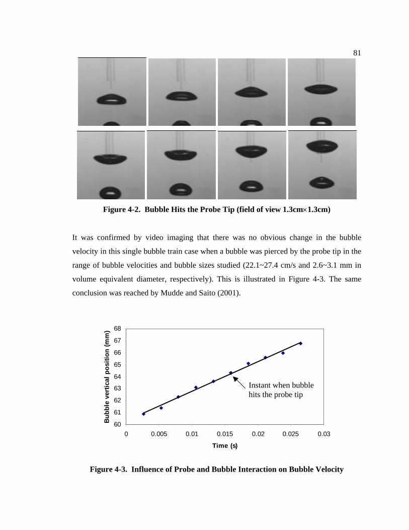
81

Figure 4-2. Bubble Hits the Probe Tip (field of view 1.3cm×1.3cm)

It was confirmed by video imaging that there was no obvious change in the bubble

velocity in this single bubble train case when a bubble was pierced by the probe tip in the

range of bubble velocities and bubble sizes studied (22.1~27.4 cm/s and 2.6~3.1 mm in

volume equivalent diameter, respectively). This is illustrated in Figure 4-3. The same

conclusion was reached by Mudde and Saito (2001).

60

61

62

63

64

65

66

67

68

0 0.005 0.01 0.015 0.02 0.025 0.03

Time (s)

Bub

ble

verti

cal p

ositi

on (m

m)

Instant when bubble hits the probe tip

Figure 4-3. Influence of Probe and Bubble Interaction on Bubble Velocity

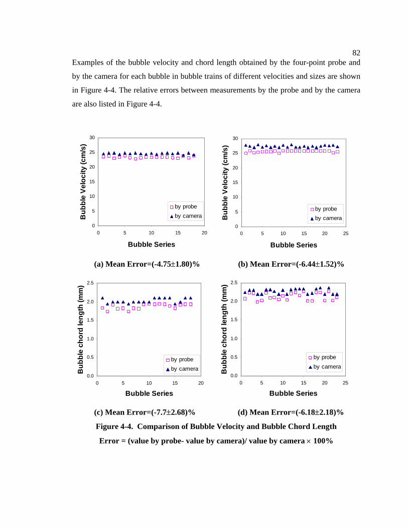
82Examples of the bubble velocity and chord length obtained by the four-point probe and

by the camera for each bubble in bubble trains of different velocities and sizes are shown

in Figure 4-4. The relative errors between measurements by the probe and by the camera

are also listed in Figure 4-4.

0

5

10

15

20

25

30

0 5 10 15 20

Bubble Series

Bub

ble

Velo

city

(cm

/s)

by probeby camera

0

5

10

15

20

25

30

0 5 10 15 20 25

Bubble Series

Bub

ble

Velo

city

(cm

/s)

by probeby camera

(a) Mean Error=(-4.75±1.80)% (b) Mean Error=(-6.44±1.52)%

0.0

0.5

1.0

1.5

2.0

2.5

0 5 10 15 20

Bubble Series

Bub

ble

chor

d le

ngth

(mm

)

by probeby camera

0.0

0.5

1.0

1.5

2.0

2.5

0 5 10 15 20 25

Bubble Series

Bub

ble

chor

d le

ngth

(mm

)

by probeby camera

(c) Mean Error=(-7.7±2.68)% (d) Mean Error=(-6.18±2.18)%

Figure 4-4. Comparison of Bubble Velocity and Bubble Chord Length

Error = (value by probe- value by camera)/ value by camera × 100%

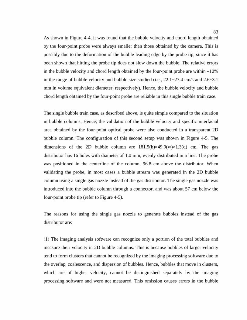
83As shown in Figure 4-4, it was found that the bubble velocity and chord length obtained

by the four-point probe were always smaller than those obtained by the camera. This is

possibly due to the deformation of the bubble leading edge by the probe tip, since it has

been shown that hitting the probe tip does not slow down the bubble. The relative errors

in the bubble velocity and chord length obtained by the four-point probe are within –10%

in the range of bubble velocity and bubble size studied (i.e., 22.1~27.4 cm/s and 2.6~3.1

mm in volume equivalent diameter, respectively). Hence, the bubble velocity and bubble

chord length obtained by the four-point probe are reliable in this single bubble train case.

The single bubble train case, as described above, is quite simple compared to the situation

in bubble columns. Hence, the validation of the bubble velocity and specific interfacial

area obtained by the four-point optical probe were also conducted in a transparent 2D

bubble column. The configuration of this second setup was shown in Figure 4-5. The

dimensions of the 2D bubble column are 181.5(h)×49.0(w)×1.3(d) cm. The gas

distributor has 16 holes with diameter of 1.0 mm, evenly distributed in a line. The probe

was positioned in the centerline of the column, 96.8 cm above the distributor. When

validating the probe, in most cases a bubble stream was generated in the 2D bubble

column using a single gas nozzle instead of the gas distributor. The single gas nozzle was

introduced into the bubble column through a connector, and was about 57 cm below the

four-point probe tip (refer to Figure 4-5).

The reasons for using the single gas nozzle to generate bubbles instead of the gas

distributor are:

(1) The imaging analysis software can recognize only a portion of the total bubbles and

measure their velocity in 2D bubble columns. This is because bubbles of larger velocity

tend to form clusters that cannot be recognized by the imaging processing software due to

the overlap, coalescence, and dispersion of bubbles. Hence, bubbles that move in clusters,

which are of higher velocity, cannot be distinguished separately by the imaging

processing software and were not measured. This omission causes errors in the bubble

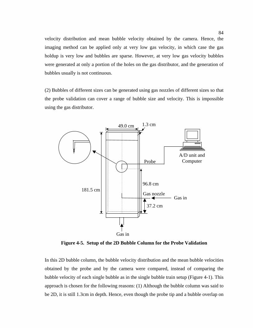
84velocity distribution and mean bubble velocity obtained by the camera. Hence, the

imaging method can be applied only at very low gas velocity, in which case the gas

holdup is very low and bubbles are sparse. However, at very low gas velocity bubbles

were generated at only a portion of the holes on the gas distributor, and the generation of

bubbles usually is not continuous.

(2) Bubbles of different sizes can be generated using gas nozzles of different sizes so that

the probe validation can cover a range of bubble size and velocity. This is impossible

using the gas distributor.

96.8 cm

1.3 cm

Probe

181.5 cm

49.0 cm

A/D unit and Computer

Gas nozzle

37.2 cm

Gas in

Gas in

Figure 4-5. Setup of the 2D Bubble Column for the Probe Validation

In this 2D bubble column, the bubble velocity distribution and the mean bubble velocities

obtained by the probe and by the camera were compared, instead of comparing the

bubble velocity of each single bubble as in the single bubble train setup (Figure 4-1). This

approach is chosen for the following reasons: (1) Although the bubble column was said to

be 2D, it is still 1.3cm in depth. Hence, even though the probe tip and a bubble overlap on

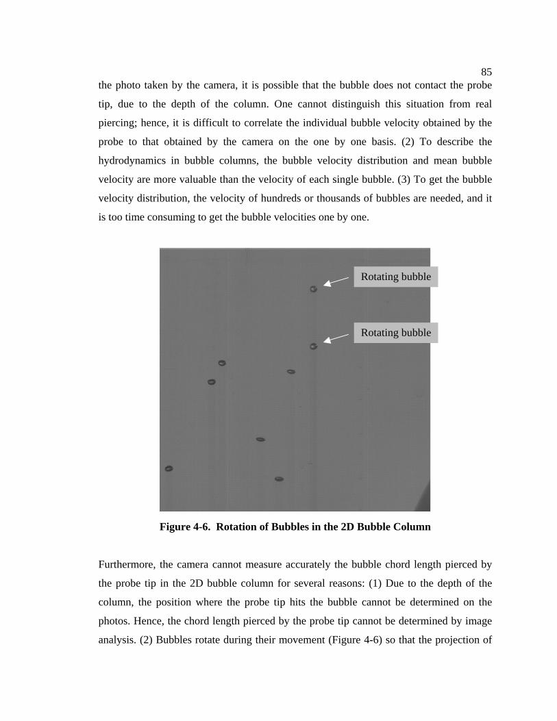
85the photo taken by the camera, it is possible that the bubble does not contact the probe

tip, due to the depth of the column. One cannot distinguish this situation from real

piercing; hence, it is difficult to correlate the individual bubble velocity obtained by the

probe to that obtained by the camera on the one by one basis. (2) To describe the

hydrodynamics in bubble columns, the bubble velocity distribution and mean bubble

velocity are more valuable than the velocity of each single bubble. (3) To get the bubble

velocity distribution, the velocity of hundreds or thousands of bubbles are needed, and it

is too time consuming to get the bubble velocities one by one.

Rotating bubble

Rotating bubble

Figure 4-6. Rotation of Bubbles in the 2D Bubble Column

Furthermore, the camera cannot measure accurately the bubble chord length pierced by

the probe tip in the 2D bubble column for several reasons: (1) Due to the depth of the

column, the position where the probe tip hits the bubble cannot be determined on the

photos. Hence, the chord length pierced by the probe tip cannot be determined by image

analysis. (2) Bubbles rotate during their movement (Figure 4-6) so that the projection of

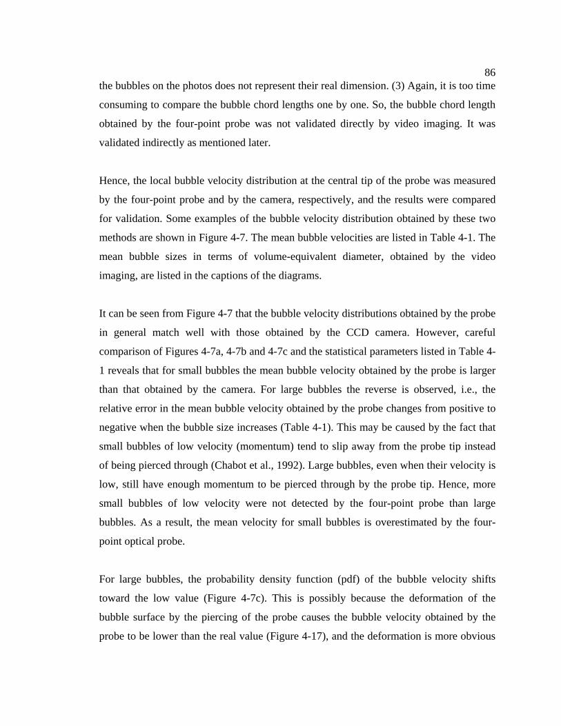
86the bubbles on the photos does not represent their real dimension. (3) Again, it is too time

consuming to compare the bubble chord lengths one by one. So, the bubble chord length

obtained by the four-point probe was not validated directly by video imaging. It was

validated indirectly as mentioned later.

Hence, the local bubble velocity distribution at the central tip of the probe was measured

by the four-point probe and by the camera, respectively, and the results were compared

for validation. Some examples of the bubble velocity distribution obtained by these two

methods are shown in Figure 4-7. The mean bubble velocities are listed in Table 4-1. The

mean bubble sizes in terms of volume-equivalent diameter, obtained by the video

imaging, are listed in the captions of the diagrams.

It can be seen from Figure 4-7 that the bubble velocity distributions obtained by the probe

in general match well with those obtained by the CCD camera. However, careful

comparison of Figures 4-7a, 4-7b and 4-7c and the statistical parameters listed in Table 4-

1 reveals that for small bubbles the mean bubble velocity obtained by the probe is larger

than that obtained by the camera. For large bubbles the reverse is observed, i.e., the

relative error in the mean bubble velocity obtained by the probe changes from positive to

negative when the bubble size increases (Table 4-1). This may be caused by the fact that

small bubbles of low velocity (momentum) tend to slip away from the probe tip instead

of being pierced through (Chabot et al., 1992). Large bubbles, even when their velocity is

low, still have enough momentum to be pierced through by the probe tip. Hence, more

small bubbles of low velocity were not detected by the four-point probe than large

bubbles. As a result, the mean velocity for small bubbles is overestimated by the four-

point optical probe.

For large bubbles, the probability density function (pdf) of the bubble velocity shifts

toward the low value (Figure 4-7c). This is possibly because the deformation of the

bubble surface by the piercing of the probe causes the bubble velocity obtained by the

probe to be lower than the real value (Figure 4-17), and the deformation is more obvious

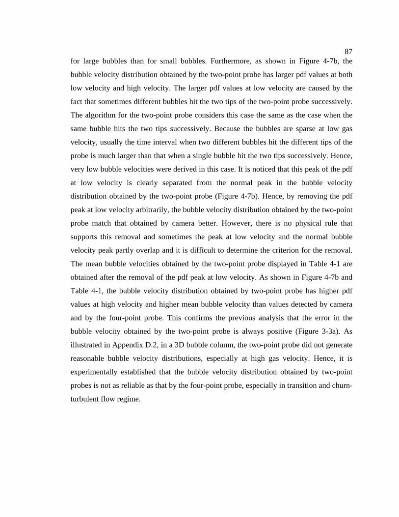
87for large bubbles than for small bubbles. Furthermore, as shown in Figure 4-7b, the

bubble velocity distribution obtained by the two-point probe has larger pdf values at both

low velocity and high velocity. The larger pdf values at low velocity are caused by the

fact that sometimes different bubbles hit the two tips of the two-point probe successively.

The algorithm for the two-point probe considers this case the same as the case when the

same bubble hits the two tips successively. Because the bubbles are sparse at low gas

velocity, usually the time interval when two different bubbles hit the different tips of the

probe is much larger than that when a single bubble hit the two tips successively. Hence,

very low bubble velocities were derived in this case. It is noticed that this peak of the pdf

at low velocity is clearly separated from the normal peak in the bubble velocity

distribution obtained by the two-point probe (Figure 4-7b). Hence, by removing the pdf

peak at low velocity arbitrarily, the bubble velocity distribution obtained by the two-point

probe match that obtained by camera better. However, there is no physical rule that

supports this removal and sometimes the peak at low velocity and the normal bubble

velocity peak partly overlap and it is difficult to determine the criterion for the removal.

The mean bubble velocities obtained by the two-point probe displayed in Table 4-1 are

obtained after the removal of the pdf peak at low velocity. As shown in Figure 4-7b and

Table 4-1, the bubble velocity distribution obtained by two-point probe has higher pdf

values at high velocity and higher mean bubble velocity than values detected by camera

and by the four-point probe. This confirms the previous analysis that the error in the

bubble velocity obtained by the two-point probe is always positive (Figure 3-3a). As

illustrated in Appendix D.2, in a 3D bubble column, the two-point probe did not generate

reasonable bubble velocity distributions, especially at high gas velocity. Hence, it is

experimentally established that the bubble velocity distribution obtained by two-point

probes is not as reliable as that by the four-point probe, especially in transition and churn-

turbulent flow regime.

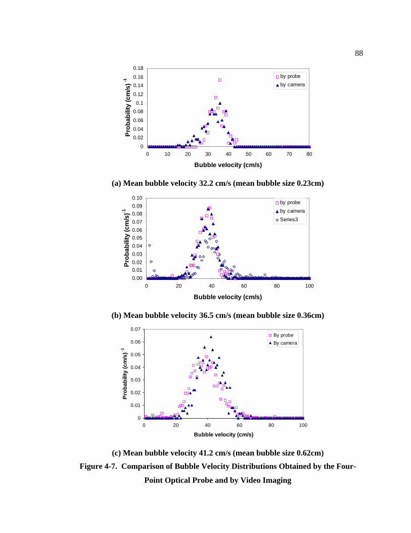
88

0

0.020.04

0.06

0.080.1

0.12

0.140.16

0.18

0 10 20 30 40 50 60 70 80

Bubble velocity (cm/s)

Prob

abili

ty (c

m/s

)-1

by probeby camera

(a) Mean bubble velocity 32.2 cm/s (mean bubble size 0.23cm)

0.000.010.020.030.040.050.060.070.080.090.10

0 20 40 60 80


Prob

abili

ty (c

m/s

)-1

100

by probeby cameraSeries3

(b) Mean bubble velocity 36.5 cm/s (mean bubble size 0.36cm)

0

0.01

0.02

0.03

0.04

0.05

0.06

0.07

0 20 40 60 80 100


Prob

abili

ty (c

m/s

)-1

By probe By camera

(c) Mean bubble velocity 41.2 cm/s (mean bubble size 0.62cm)

Figure 4-7. Comparison of Bubble Velocity Distributions Obtained by the Four-

Point Optical Probe and by Video Imaging

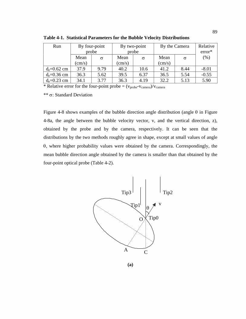
89Table 4-1. Statistical Parameters for the Bubble Velocity Distributions

By four-point probe

By two-point probe

By the Camera Run

Mean (cm/s)

σ Mean (cm/s)

σ Mean (cm/s)

σ

Relative error* (%)

de=0.62 cm 37.9 9.79 40.2 10.6 41.2 8.44 -8.01 de=0.36 cm 36.3 5.62 39.5 6.37 36.5 5.54 -0.55 de=0.23 cm 34.1 3.77 36.3 4.19 32.2 5.13 5.90

* Relative error for the four-point probe = (vprobe-vcamera)/vcamera

** σ: Standard Deviation

Figure 4-8 shows examples of the bubble direction angle distribution (angle θ in Figure

4-8a, the angle between the bubble velocity vector, v, and the vertical direction, z),

obtained by the probe and by the camera, respectively. It can be seen that the

distributions by the two methods roughly agree in shape, except at small values of angle

θ, where higher probability values were obtained by the camera. Correspondingly, the

mean bubble direction angle obtained by the camera is smaller than that obtained by the

four-point optical probe (Table 4-2).

v

Tip2

A

θ

Tip3

Tip1

Tip0O

C

(a)

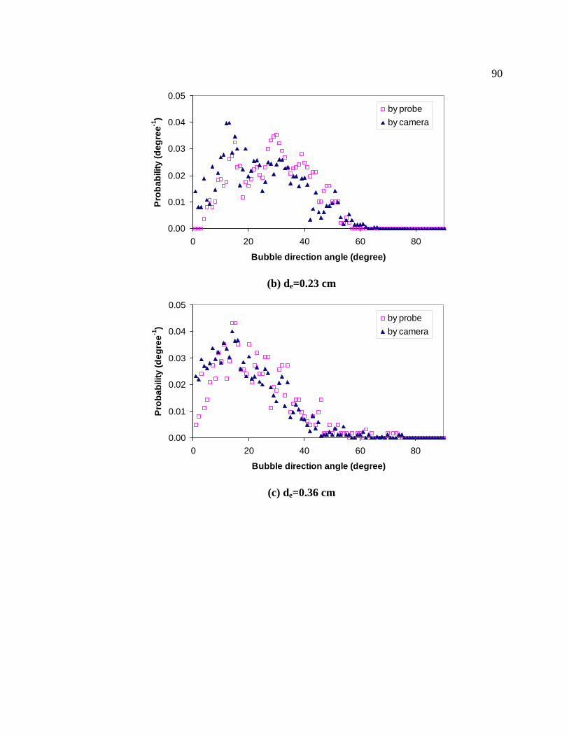
90

0.00

0.01

0.02

0.03

0.04

0.05

0 20 40 60 80

Bubble direction angle (degree)

Prob

abili

ty (d

egre

e-1)

by probeby camera

(b) de=0.23 cm

0.00

0.01

0.02

0.03

0.04

0.05

0 20 40 60 80


Prob

abili

ty (d

egre

e-1)

by probeby camera

(c) de=0.36 cm

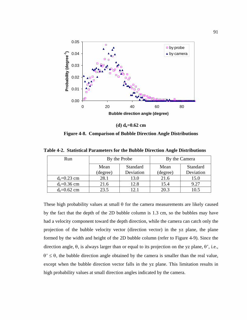
91

0.00

0.01

0.02

0.03

0.04

0.05

0 20 40 60 80


Prob

abili

ty (d

egre

e-1)

by probeby camera

(d) de=0.62 cm

Figure 4-8. Comparison of Bubble Direction Angle Distributions

Table 4-2. Statistical Parameters for the Bubble Direction Angle Distributions

By the Probe By the Camera Run

Mean (degree)

Standard Deviation

Mean (degree)

Standard Deviation

de=0.23 cm 28.1 13.0 21.6 15.0 de=0.36 cm 21.6 12.8 15.4 9.27 de=0.62 cm 23.5 12.1 20.3 10.5

These high probability values at small θ for the camera measurements are likely caused

by the fact that the depth of the 2D bubble column is 1.3 cm, so the bubbles may have

had a velocity component toward the depth direction, while the camera can catch only the

projection of the bubble velocity vector (direction vector) in the yz plane, the plane

formed by the width and height of the 2D bubble column (refer to Figure 4-9). Since the

direction angle, θ, is always larger than or equal to its projection on the yz plane, θ’, i.e.,

θ’ ≤ θ, the bubble direction angle obtained by the camera is smaller than the real value,

except when the bubble direction vector falls in the yz plane. This limitation results in

high probability values at small direction angles indicated by the camera.

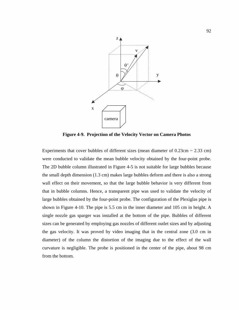
92

θ’

ϕ

x

v

z

y θ

camera

Figure 4-9. Projection of the Velocity Vector on Camera Photos

Experiments that cover bubbles of different sizes (mean diameter of 0.23cm ~ 2.33 cm)

were conducted to validate the mean bubble velocity obtained by the four-point probe.

The 2D bubble column illustrated in Figure 4-5 is not suitable for large bubbles because

the small depth dimension (1.3 cm) makes large bubbles deform and there is also a strong

wall effect on their movement, so that the large bubble behavior is very different from

that in bubble columns. Hence, a transparent pipe was used to validate the velocity of

large bubbles obtained by the four-point probe. The configuration of the Plexiglas pipe is

shown in Figure 4-10. The pipe is 5.5 cm in the inner diameter and 105 cm in height. A

single nozzle gas sparger was installed at the bottom of the pipe. Bubbles of different

sizes can be generated by employing gas nozzles of different outlet sizes and by adjusting

the gas velocity. It was proved by video imaging that in the central zone (3.0 cm in

diameter) of the column the distortion of the imaging due to the effect of the wall

curvature is negligible. The probe is positioned in the center of the pipe, about 98 cm

from the bottom.

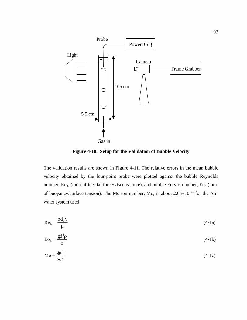
93

PowerDAQ

Gas in

Frame GrabberCamera

Light

5.5 cm

105 cm

Probe

Figure 4-10. Setup for the Validation of Bubble Velocity

The validation results are shown in Figure 4-11. The relative errors in the mean bubble

velocity obtained by the four-point probe were plotted against the bubble Reynolds

number, Reb, (ratio of inertial force/viscous force), and bubble Eotvos number, Eob (ratio

of buoyancy/surface tension). The Morton number, Mo, is about 2.65×10-11 for the Air-

water system used:

µρ

=vd

Re eb (4-1a)

σρ

=2e

bgdEo (4-1b)

3

4gMoρσµ

= (4-1c)

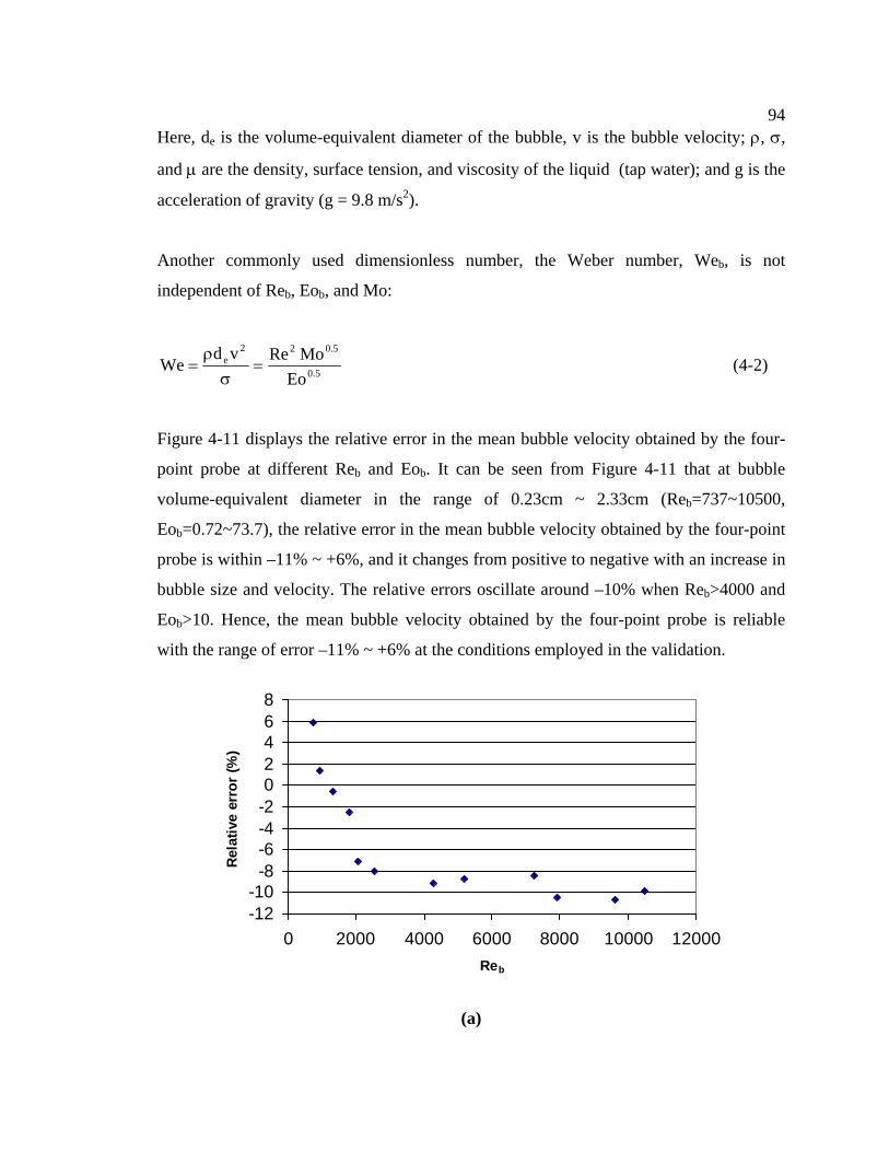
94Here, de is the volume-equivalent diameter of the bubble, v is the bubble velocity; ρ, σ,

and µ are the density, surface tension, and viscosity of the liquid (tap water); and g is the

acceleration of gravity (g = 9.8 m/s2).

Another commonly used dimensionless number, the Weber number, Web, is not

independent of Reb, Eob, and Mo:

5.0

5.022e

EoMoRevd

We =σ

ρ= (4-2)

Figure 4-11 displays the relative error in the mean bubble velocity obtained by the four-

point probe at different Reb and Eob. It can be seen from Figure 4-11 that at bubble

volume-equivalent diameter in the range of 0.23cm ~ 2.33cm (Reb=737~10500,

Eob=0.72~73.7), the relative error in the mean bubble velocity obtained by the four-point

probe is within –11% ~ +6%, and it changes from positive to negative with an increase in

bubble size and velocity. The relative errors oscillate around –10% when Reb>4000 and

Eob>10. Hence, the mean bubble velocity obtained by the four-point probe is reliable

with the range of error –11% ~ +6% at the conditions employed in the validation.

-12-10

-8-6-4-202468

0 2000 4000 6000 8000 10000 12000Reb

Rel

ativ

e er

ror

(%)

(a)

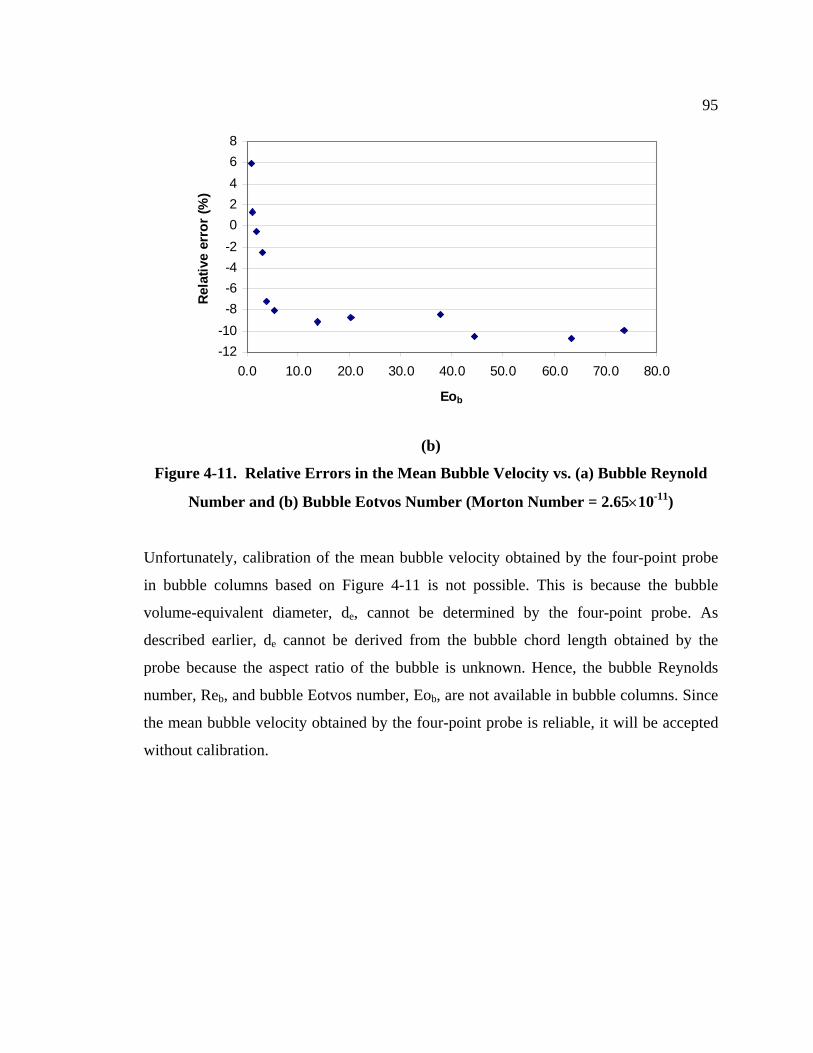
95

-12-10-8-6-4-202468

0.0 10.0 20.0 30.0 40.0 50.0 60.0 70.0 80.0

Eob

Rela

tive

erro

r (%

)

(b)

Figure 4-11. Relative Errors in the Mean Bubble Velocity vs. (a) Bubble Reynold

Number and (b) Bubble Eotvos Number (Morton Number = 2.65×10-11)

Unfortunately, calibration of the mean bubble velocity obtained by the four-point probe

in bubble columns based on Figure 4-11 is not possible. This is because the bubble

volume-equivalent diameter, de, cannot be determined by the four-point probe. As

described earlier, de cannot be derived from the bubble chord length obtained by the

probe because the aspect ratio of the bubble is unknown. Hence, the bubble Reynolds

number, Reb, and bubble Eotvos number, Eob, are not available in bubble columns. Since

the mean bubble velocity obtained by the four-point probe is reliable, it will be accepted

without calibration.

964.2 Validation of the Specific Interfacial Area

In the case of spherical bubbles, the relationship between the specific interfacial area and

the bubble size distribution is simple, and can be described by (Patel, Daly and Bukur,

1989):

s

g

d6

aε

= (4-3)

In Equation (4-3), a is the specific interfacial area, εg is the gas holdup, and ds is the

Sauter mean diameter (the average volume-surface mean diameter of bubbles) as

described in Equation (2-2).

It is well known that most bubbles are not spherical in most practical multiphase systems.

When bubbles are not spherical, e.g., ellipsoidal, the relationship between the specific

interfacial area and the bubble size distribution is much more complicated than Equation

(4-3). Assume that the ellipsoidal bubble has two major axes, c, and one minor axis, b.

The three axes of an ellipsoidal bubble are c, c, b, where c>b, and α=b/c is the aspect

ratio of the bubble. Then the surface area of the bubble is:

⎥⎥⎦

⎤

⎢⎢⎣

⎡

⎟⎟⎠

⎞⎜⎜⎝

⎛

αα−+

α−

α+π=

⎥⎥⎦

⎤

⎢⎢⎣

⎡

⎟⎟⎠

⎞⎜⎜⎝

⎛ −+

−+π=

2

2

22

22

22

22 11ln

11c8

bbccln

bccbc8S (4-4)

The volume of the bubble is:

32 c3

4bc3

4V απ

=π

= (4-5)

97Hence, the specific interfacial area is:

∑= ⎥

⎥

⎦

⎤

⎢⎢

⎣

⎡

⎟⎟

⎠

⎞

⎜⎜

⎝

⎛

αα−+

α−

α+π=

Ni i

2i

2i

2i2

i

11ln

11c8a (4-6)

where N is the average number of bubbles in unit volume.

The gas holdup is then given by:

∑=

απ

=εNi

3iig c

34 (4-7)

Since the aspect ratios of bubbles in bubble columns are not identical, it is evident from

Equations (4-6) and (4-7) that there is no simple correlation between mean bubble size,

gas holdup and specific interfacial area for ellipsoidal bubbles, let alone bubbles of

irregular shape. Furthermore, for ellipsoidal bubbles Equation (4-3) does not hold even

when the aspect ratio of bubbles is identical. Assuming that the size and aspect ratio of

all bubbles in bubble columns are identical, Figure 4-12 shows the relative error in the

specific interfacial area calculated according to Equation (4-3). It can be seen that

Equation (4-3) always underestimates the interfacial area. The smaller the aspect ratio,

the larger the relative error. In other words, the more the bubble shape deviates from

spherical, the larger the relative error in the specific interfacial area obtained by Equation

(4-3). The relative error is –55% at aspect ratio α=0.5, and becomes about –100% when

α goes to zero. In the case of different bubble sizes and aspect ratios for the whole bubble

population, the relative error in the specific interfacial area is the combination of that

shown in Figure 4-12, and is expected to be of the same order of magnitude as that shown

in Figure 4-12. It is obvious by this simulation that the error in the specific interfacial

obtained by Equation (4-3) may be very large for nonspherical bubbles. Hence, Equation

(4-3) is an oversimplification for practical multiphase systems, and it can be treated only

as a rough estimate of the specific interfacial area and Sauter mean bubble diameter.

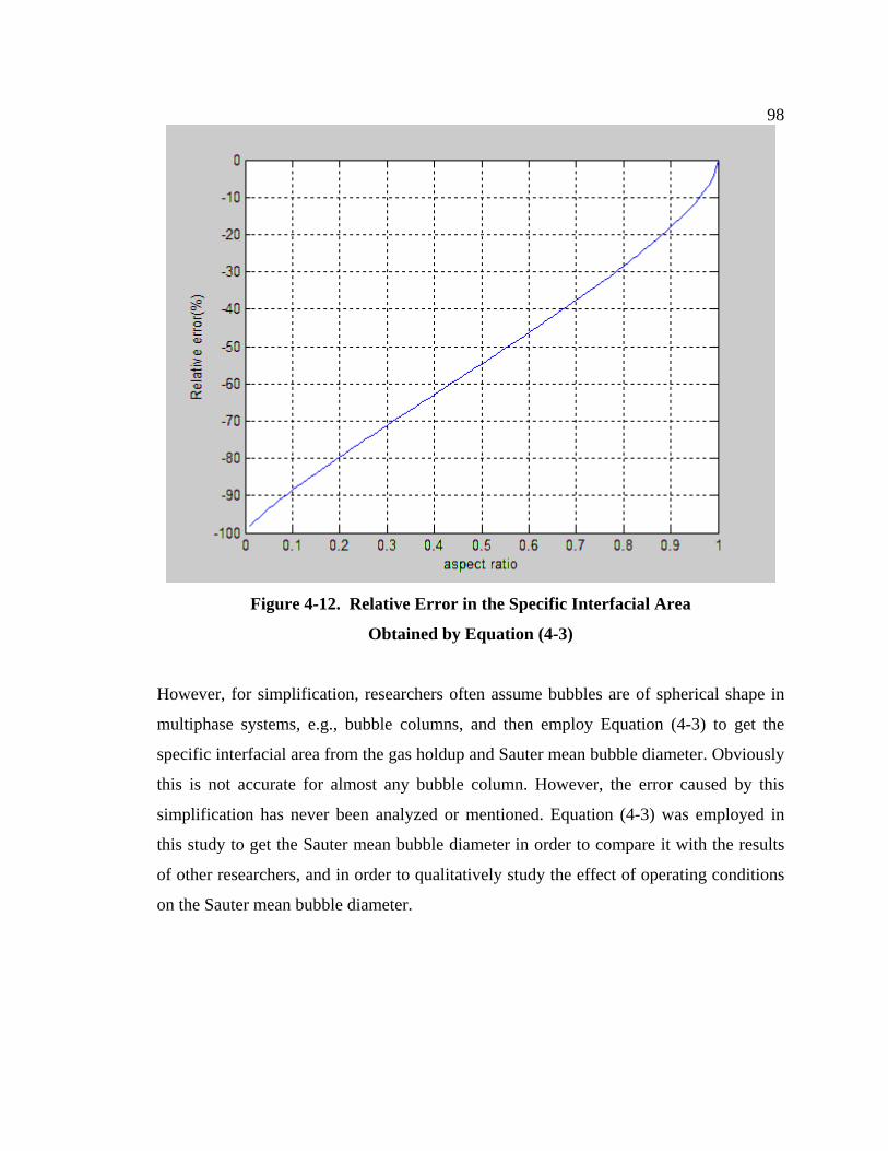
98

Figure 4-12. Relative Error in the Specific Interfacial Area

Obtained by Equation (4-3)

However, for simplification, researchers often assume bubbles are of spherical shape in

multiphase systems, e.g., bubble columns, and then employ Equation (4-3) to get the

specific interfacial area from the gas holdup and Sauter mean bubble diameter. Obviously

this is not accurate for almost any bubble column. However, the error caused by this

simplification has never been analyzed or mentioned. Equation (4-3) was employed in

this study to get the Sauter mean bubble diameter in order to compare it with the results

of other researchers, and in order to qualitatively study the effect of operating conditions

on the Sauter mean bubble diameter.

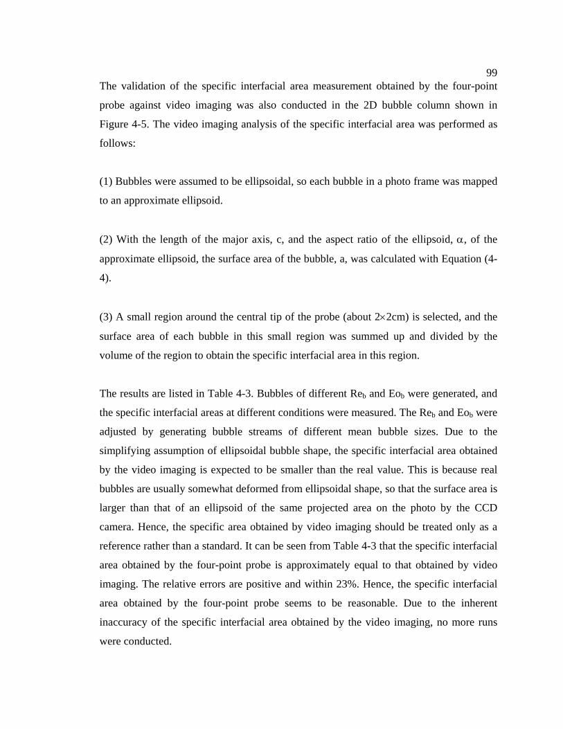
99The validation of the specific interfacial area measurement obtained by the four-point

probe against video imaging was also conducted in the 2D bubble column shown in

Figure 4-5. The video imaging analysis of the specific interfacial area was performed as

follows:

(1) Bubbles were assumed to be ellipsoidal, so each bubble in a photo frame was mapped

to an approximate ellipsoid.

(2) With the length of the major axis, c, and the aspect ratio of the ellipsoid, α, of the

approximate ellipsoid, the surface area of the bubble, a, was calculated with Equation (4-

4).

(3) A small region around the central tip of the probe (about 2×2cm) is selected, and the

surface area of each bubble in this small region was summed up and divided by the

volume of the region to obtain the specific interfacial area in this region.

The results are listed in Table 4-3. Bubbles of different Reb and Eob were generated, and

the specific interfacial areas at different conditions were measured. The Reb and Eob were

adjusted by generating bubble streams of different mean bubble sizes. Due to the

simplifying assumption of ellipsoidal bubble shape, the specific interfacial area obtained

by the video imaging is expected to be smaller than the real value. This is because real

bubbles are usually somewhat deformed from ellipsoidal shape, so that the surface area is

larger than that of an ellipsoid of the same projected area on the photo by the CCD

camera. Hence, the specific area obtained by video imaging should be treated only as a

reference rather than a standard. It can be seen from Table 4-3 that the specific interfacial

area obtained by the four-point probe is approximately equal to that obtained by video

imaging. The relative errors are positive and within 23%. Hence, the specific interfacial

area obtained by the four-point probe seems to be reasonable. Due to the inherent

inaccuracy of the specific interfacial area obtained by the video imaging, no more runs

were conducted.

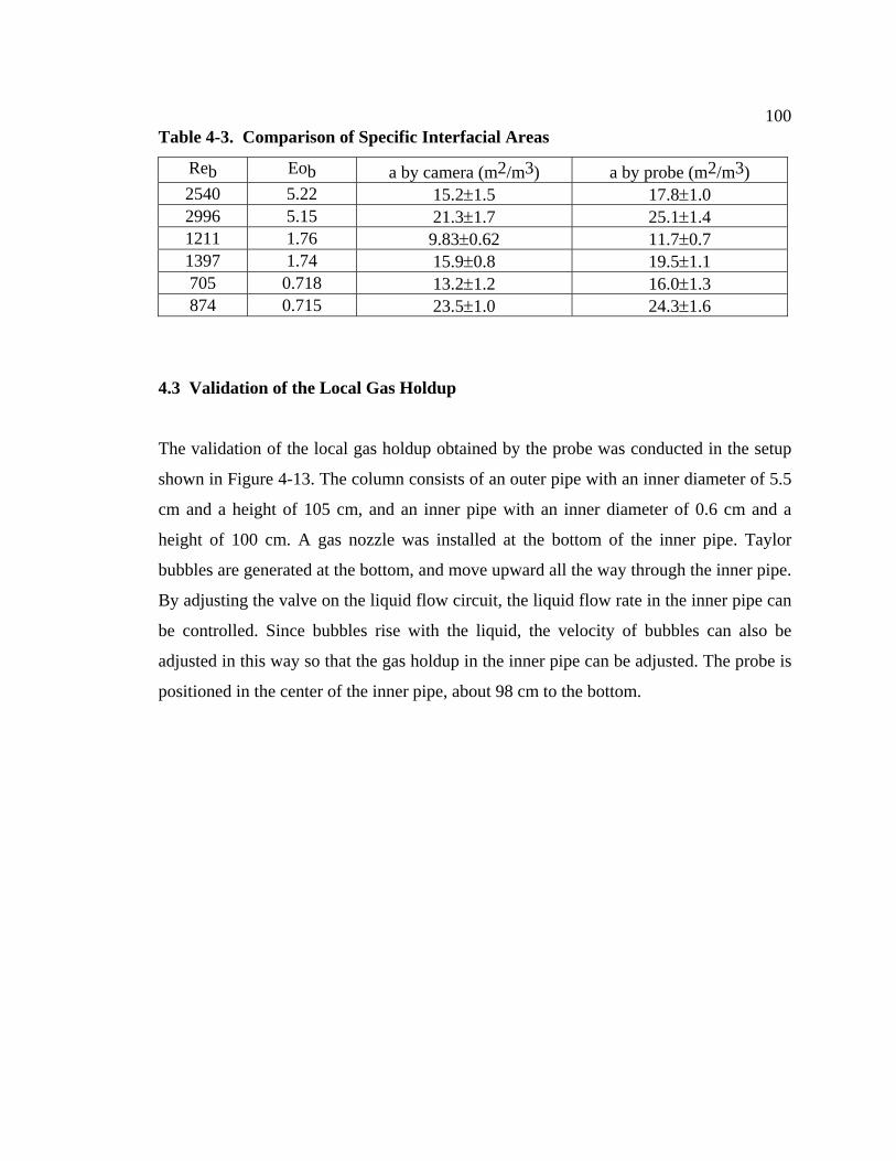
100Table 4-3. Comparison of Specific Interfacial Areas

Reb Eob a by camera (m2/m3) a by probe (m2/m3) 2540 5.22 15.2±1.5 17.8±1.0 2996 5.15 21.3±1.7 25.1±1.4 1211 1.76 9.83±0.62 11.7±0.7 1397 1.74 15.9±0.8 19.5±1.1 705 0.718 13.2±1.2 16.0±1.3 874 0.715 23.5±1.0 24.3±1.6

4.3 Validation of the Local Gas Holdup

The validation of the local gas holdup obtained by the probe was conducted in the setup

shown in Figure 4-13. The column consists of an outer pipe with an inner diameter of 5.5

cm and a height of 105 cm, and an inner pipe with an inner diameter of 0.6 cm and a

height of 100 cm. A gas nozzle was installed at the bottom of the inner pipe. Taylor

bubbles are generated at the bottom, and move upward all the way through the inner pipe.

By adjusting the valve on the liquid flow circuit, the liquid flow rate in the inner pipe can

be controlled. Since bubbles rise with the liquid, the velocity of bubbles can also be

adjusted in this way so that the gas holdup in the inner pipe can be adjusted. The probe is

positioned in the center of the inner pipe, about 98 cm to the bottom.

101

PowerDAQ

Liquid flow Gas in

Frame GrabberCamera

Light

Valve

5.5 cm0.6 cm

Taylor bubble

Figure 4-13. Setup for the Validation of Local Gas Holdup

It is important to recognize that the gas holdup obtained by the probe, which is time

based, is a little different from the volume based gas holdup, which is commonly used.

The definition of volume based gas holdup is that it is the fraction of the whole

multiphase system volume that is occupied by the gas phase. Based on this definition, the

overall gas holdup in bubble columns can be measured using the bed expansion method

as follows:

D

ID

GL

GGV,g H

HHVV

VV

V −=

+==ε (4-8)

where VG is the volume occupied by the gas phase (bubbles), VL is the volume occupied

by the liquid phase, V is the total volume of the gas-liquid mixed phase, HI is the initial

liquid phase height, and HD is the dynamic height of the gas-liquid system.

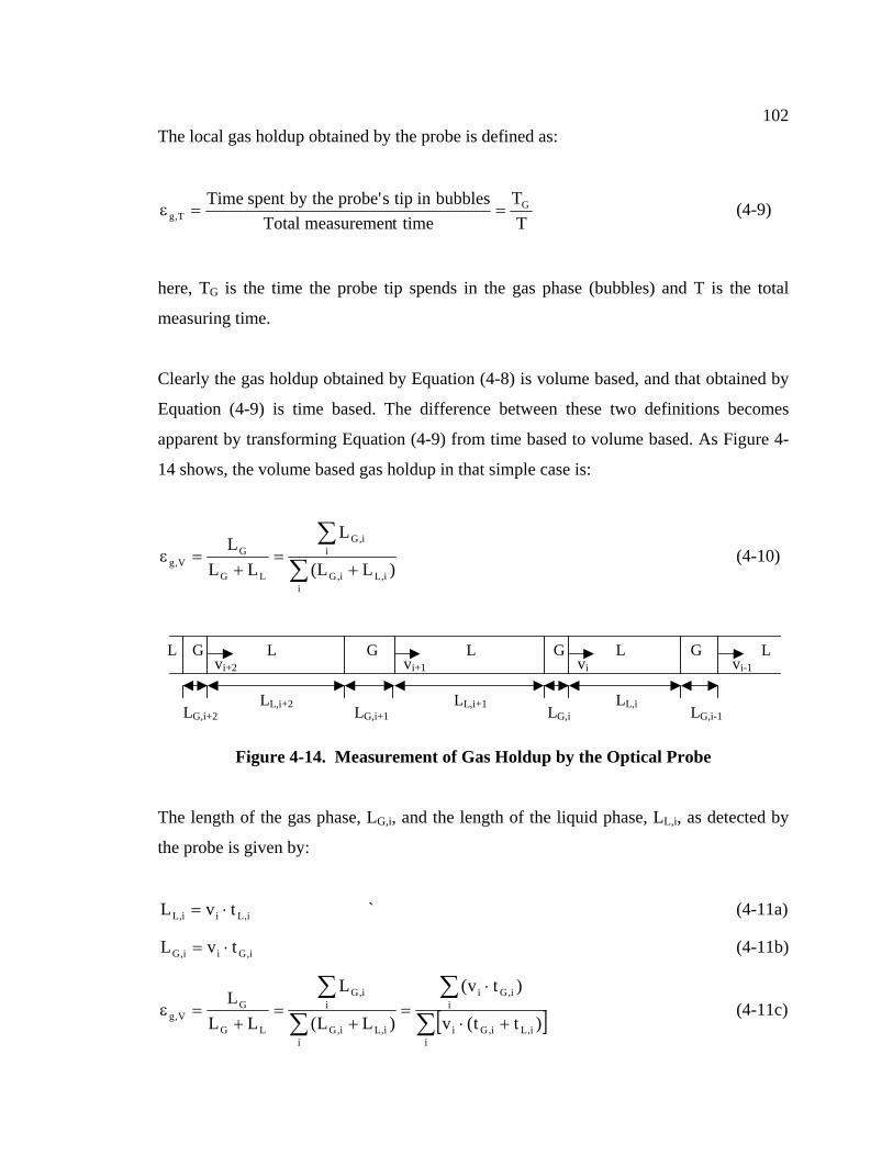
102The local gas holdup obtained by the probe is defined as:

TT

timetmeasuremenTotalbubblesintips'probethebyspentTime G

T,g ==ε (4-9)

here, TG is the time the probe tip spends in the gas phase (bubbles) and T is the total

measuring time.

Clearly the gas holdup obtained by Equation (4-8) is volume based, and that obtained by

Equation (4-9) is time based. The difference between these two definitions becomes

apparent by transforming Equation (4-9) from time based to volume based. As Figure 4-

14 shows, the volume based gas holdup in that simple case is:

∑∑

+=

+=ε

ii,Li,G

ii,G

LG

GV,g )LL(

L

LLL

(4-10)

G G G G L L L LL

LL,i+2 LG,i+2 LG,i+1 LG,i LG,i-1LL,i+1 LL,i

vi-1 vi vi+1 vi+2

Figure 4-14. Measurement of Gas Holdup by the Optical Probe

The length of the gas phase, LG,i, and the length of the liquid phase, LL,i, as detected by

the probe is given by:

i,Lii,L tvL ⋅= ` (4-11a)

i,Gii,G tvL ⋅= (4-11b)

[ ]∑∑

∑∑

+⋅

⋅=

+=

+=ε

ii,Li,Gi

ii,Gi

ii,Li,G

ii,G

LG

GV,g )tt(v

)tv(

)LL(

L

LLL

(4-11c)

103In Equation (4-11c), vi is the velocity of the ith gas-liquid interface (bubble leading

phase), tG,i is the time interval that the probe tip spends in the ith gas section (bubble),

and tL,i is the time interval that the probe tip spends in the ith liquid section.

According to the calculus of random variables (Bruce, 1985), if vi and tG,i are

independent, then:

( ) ( ) ∞→⋅=⋅∑ NwhentvNtv Gi

i,Gi (4-12)

where v and Gt are the mean gas-liquid interface velocity and mean time interval that

the probe tip spends in the gas sections, respectively.

From Equation (4-12) it can be derived that if vi are statistically independent of tG,i and

tL,i, then:

( ) ( ) ∞→⋅=⋅=⋅ ∑∑ NwhentvtvNtvi

i,GGi

i,Gi (4-13a)

( ) ( ) ∞→⋅=⋅=⋅ ∑∑ NwhentvtvNtvi

i,LLi

i,Li (4-13b)

( )[ ] T

T)tt(

t

)tt(v

tvG

ii,Li,G

ii,G

ii,Li,Gi

ii,Gi

V,g =+

=+⋅

⋅=ε

∑∑

∑∑

(4-13c)

Hence, Equation (4-9) is the same as Equation (4-8) only if vi are independent of tG,i and

tL,i and the number of bubbles passing by the probe tip during the measurement is large

enough.

104It can also be derived that:

( ) [ ]

( ) ∑∑∑

∑∑∑∑

∑∑

∆⋅∆+⋅=

∆⋅∆+⋅=

∆⋅+∆⋅+∆⋅∆+⋅=

∆+⋅∆+=⋅

ii,GiG

ii,Gi

iG

iiG

ii,G

ii,Gi

iG

ii,GGi

ii,Gi

)tv(tvN

)tv()tv(

)vt()tv()tv()tv(

)tt()vv(tv

(4-14)

where and are the fluctuations in gas-liquid interface velocity and in the time

interval that the probe tip spends in the gas sections, respectively.

iv∆ i,Gt∆

Hence, when v0)tv(i

i,Gi =∆⋅∆∑ i and tG,i are statistically independent. However, in

bubble columns vi are not independent of tG,i and tL,i because large bubbles move faster

than small bubbles in bubble columns, so a large value of tG,i corresponds to a large vi.

Thus, a positive value of tends to correlate to a positive iv∆ i,Gt∆ , and vice versa. This

correlation implies that the fluctuation term in Equation (4-14) is positive in most cases,

and Equation (4-13c) does not hold. However, it was found that in bubble columns

operated in churn-turbulent flow some small bubbles also exhibit large velocities because

they move with the wake of the large bubbles. In such a case, a positive value of iv∆

correlates to negative . These two tendencies counteract, and Equation (4-13) is

approximately acceptable because the behavior of small bubbles is decisive in Equation

(4-13), due to the overwhelming number of small bubbles compared to large bubbles.

Furthermore, the ∑ term appears in both the denominator and the numerator of

Equation (4-13c), counteracting the correlation of v

i,Gt∆

⋅i

i,Gi )tv(

i and tG,i to some extent. Hence, it is

expected that the difference between these two definitions of gas holdup is not substantial

in bubble columns.

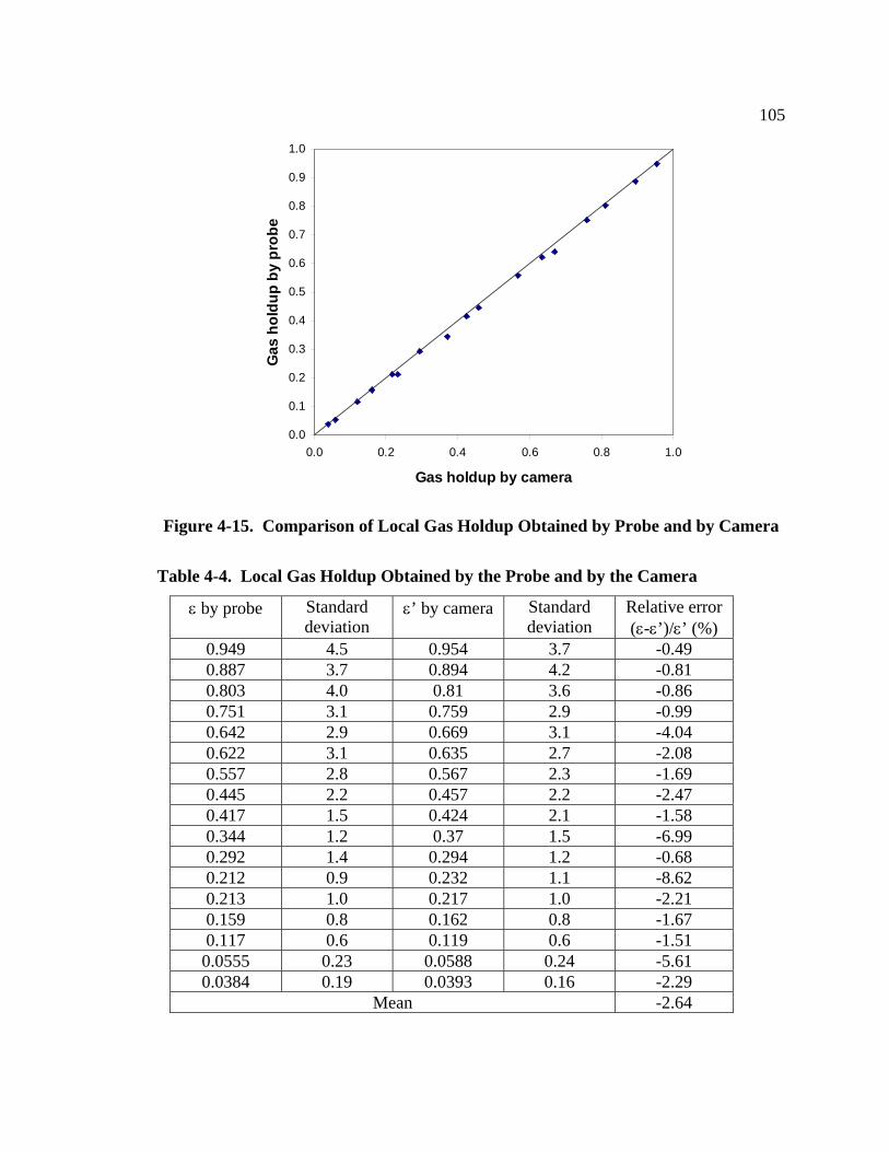
105

0.0

0.1

0.2

0.3

0.4

0.5

0.6

0.7

0.8

0.9

1.0

0.0 0.2 0.4 0.6 0.8 1.0

Gas holdup by camera

Gas

hol

dup

by p

robe

Figure 4-15. Comparison of Local Gas Holdup Obtained by Probe and by Camera

Table 4-4. Local Gas Holdup Obtained by the Probe and by the Camera

ε by probe

Standard deviation

ε’ by camera

Standard deviation

Relative error (ε-ε’)/ε’ (%)

0.949 4.5 0.954 3.7 -0.49 0.887 3.7 0.894 4.2 -0.81 0.803 4.0 0.81 3.6 -0.86 0.751 3.1 0.759 2.9 -0.99 0.642 2.9 0.669 3.1 -4.04 0.622 3.1 0.635 2.7 -2.08 0.557 2.8 0.567 2.3 -1.69 0.445 2.2 0.457 2.2 -2.47 0.417 1.5 0.424 2.1 -1.58 0.344 1.2 0.37 1.5 -6.99 0.292 1.4 0.294 1.2 -0.68 0.212 0.9 0.232 1.1 -8.62 0.213 1.0 0.217 1.0 -2.21 0.159 0.8 0.162 0.8 -1.67 0.117 0.6 0.119 0.6 -1.51 0.0555 0.23 0.0588 0.24 -5.61 0.0384 0.19 0.0393 0.16 -2.29

Mean -2.64

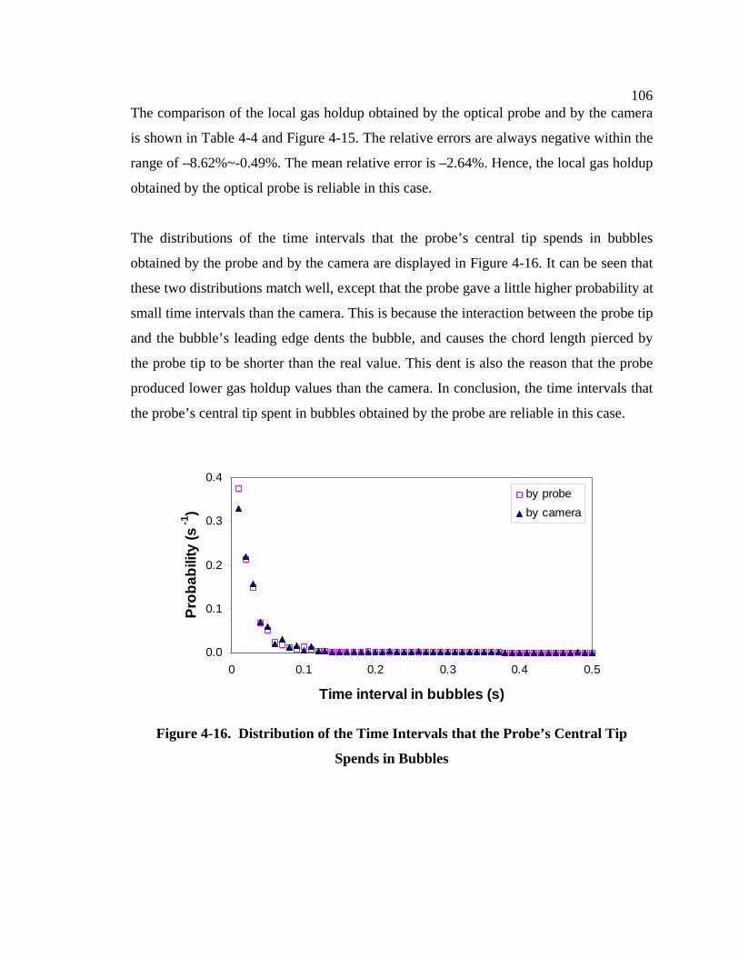
106The comparison of the local gas holdup obtained by the optical probe and by the camera

is shown in Table 4-4 and Figure 4-15. The relative errors are always negative within the

range of –8.62%~-0.49%. The mean relative error is –2.64%. Hence, the local gas holdup

obtained by the optical probe is reliable in this case.

The distributions of the time intervals that the probe’s central tip spends in bubbles

obtained by the probe and by the camera are displayed in Figure 4-16. It can be seen that

these two distributions match well, except that the probe gave a little higher probability at

small time intervals than the camera. This is because the interaction between the probe tip

and the bubble’s leading edge dents the bubble, and causes the chord length pierced by

the probe tip to be shorter than the real value. This dent is also the reason that the probe

produced lower gas holdup values than the camera. In conclusion, the time intervals that

the probe’s central tip spent in bubbles obtained by the probe are reliable in this case.

0.0

0.1

0.2

0.3

0.4

0 0.1 0.2 0.3 0.4 0.5

Time interval in bubbles (s)

Prob

abili

ty (s

-1)

by probeby camera

Figure 4-16. Distribution of the Time Intervals that the Probe’s Central Tip

Spends in Bubbles

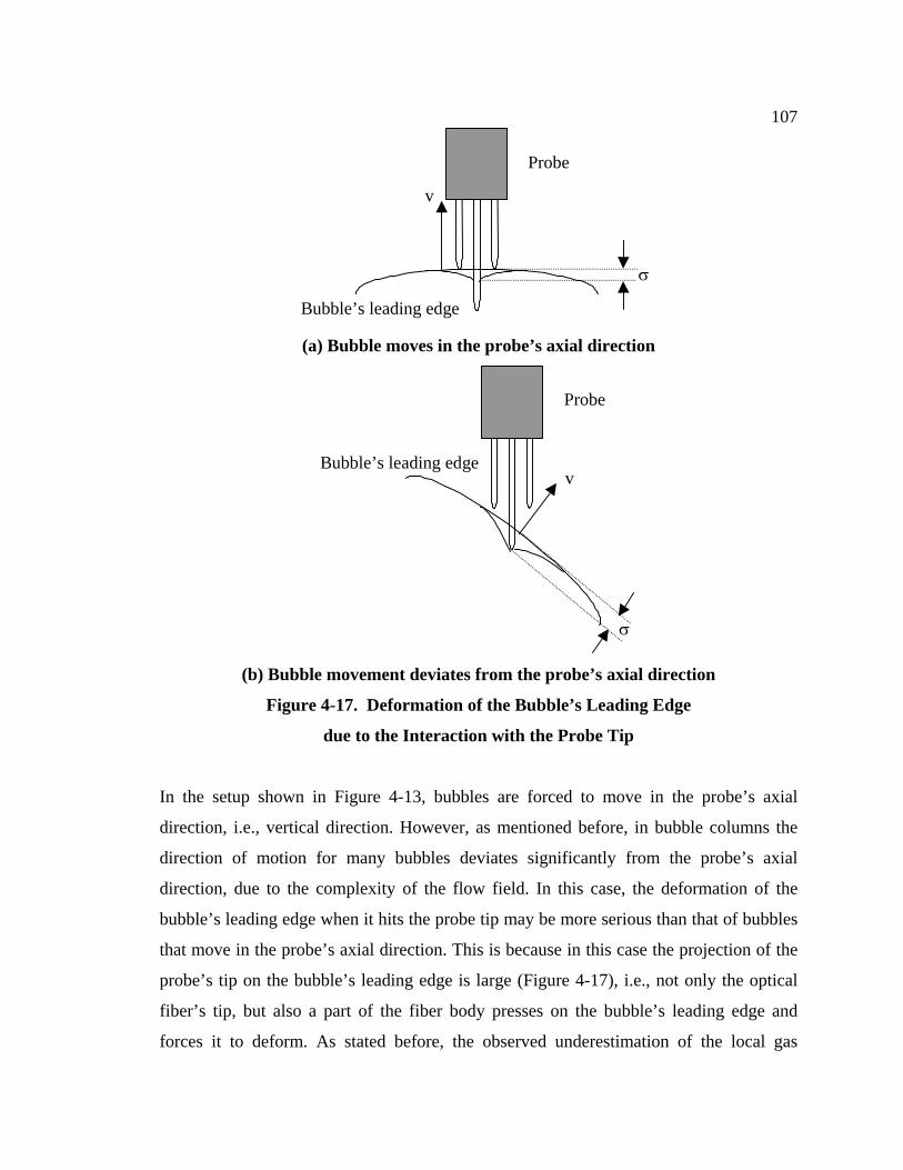
107

σ

Bubble’s leading edge

Probe

v

(a) Bubble moves in the probe’s axial direction

σ

Bubble’s leading edge

Probe

v

(b) Bubble movement deviates from the probe’s axial direction

Figure 4-17. Deformation of the Bubble’s Leading Edge

due to the Interaction with the Probe Tip

In the setup shown in Figure 4-13, bubbles are forced to move in the probe’s axial

direction, i.e., vertical direction. However, as mentioned before, in bubble columns the

direction of motion for many bubbles deviates significantly from the probe’s axial

direction, due to the complexity of the flow field. In this case, the deformation of the

bubble’s leading edge when it hits the probe tip may be more serious than that of bubbles

that move in the probe’s axial direction. This is because in this case the projection of the

probe’s tip on the bubble’s leading edge is large (Figure 4-17), i.e., not only the optical

fiber’s tip, but also a part of the fiber body presses on the bubble’s leading edge and

forces it to deform. As stated before, the observed underestimation of the local gas

108holdup is possibly caused by the deformation of the bubble’s leading edge. Hence, it is

expected that larger deformation of the bubble’s leading edge causes larger error in the

local gas holdup obtained by the probe.

Furthermore, in the setup shown in Figure 4-13, bubbles are restricted in the inner pipe,

so there is no room for bubbles to slip away from the probe’s tip. This is different from

the condition in bubble columns, where small bubbles may avoid the probe tip, due to the

disturbance of the flow field by the probe (Chabot et al., 1992). Hence, it is expected that

the error in the local gas holdup obtained by the four-point probe in bubble columns will

still be negative, and the relative errors are larger than those shown in Table 4-4. This is

proved by the experiments conducted in a 3D bubble column as described later.

The 2D bubble column is not suitable for the validation of the local gas holdup obtained

by the probe. This is because in the 2D bubble column, the local gas holdup obtained by

the camera is not accurate in the case of non-spherical bubbles, due to several factors: (1)

To extract the local gas holdup by the camera, one needs to assume the shape of bubbles,

e.g., to be ellipsoidal, and get the volume of bubbles from their projection on the CCD

plane. Obviously the bubble volume obtained in this way is not accurate for deformed

bubbles. (2) When the major symmetry plane of bubbles (the symmetry plane that

contains the major axes of an ellipsoidal bubble) is not vertical to the CCD plane (this is

common, especially for small bubbles, which rotate continuously during their rise), the

profile of bubbles obtained will be larger than the real value (refer to Figure 4-5).

Moreover, as mentioned before, the local gas holdup cannot be determined in the 2D

bubble column at relatively high gas holdup, as in bubble columns, due to the overlap of

bubbles. Hence, the verification of the local gas holdup obtained by the probe was not

conducted in the 2D bubble column.

As described before, the bubble chord lengths being pierced by the probe cannot be

derived accurately by the camera in the 2D bubble column. However, the bubble chord

length is obtained by the product of the bubble velocity, v, and the time interval that a

109probe tip spent in that bubble, Ti: ii TvL ⋅= . Hence, it is reasonable to assert that after the

validation of the bubble velocity and the time intervals that a probe tip spent in bubbles,

the bubble chord lengths obtained by the probe are also indirectly validated.

In conclusion, the validation against video imaging shows that the bubble velocity

distribution, mean bubble velocity, bubble chord length distribution, specific interfacial

area, and local gas holdup obtained by the four-point optical probe are reliable. Hence,

the probe is applied in bubble columns at different operating conditions to investigate

bubble properties in systems of practical interest.

110

Chapter 5 Bubble Properties in Bubble Columns

Obtained by the Four-Point Optical Probe

After validation of the four-point optical probe measurements in 2D systems, the probe

was utilized in 3D bubble columns under specified operating conditions of interest to

measure the bubble velocity distribution, bubble chord length distribution, local gas

holdup, and specific interfacial area.

5.1 Experimental Setup

The configuration of the 16.2 cm (6.4”) diameter stainless steel bubble column is shown

in Figure 5-1. The setup was operated in the batch mode with tap water as the liquid

phase and filtered, dry compressed air as the gas phase. The four-point probe

measurements were conducted at different gas velocities and at atmospheric and high

pressures. The operating conditions employed are listed in Table 5-1. Three axial

positions, i.e., z/D= 1.7, 5.1, and 8.5, and seven radial positions, i.e., r/R=±0.9, r/R=±0.6,

r/R=±0.3 and r/R=0, (where positive and negative values of r/R represent different sides

along the diameter of the column in the plane of measurement, Figure 5-1), were selected

for measurements of the local bubble properties. The optical probe must employ the fixed

ports on the column wall. Due to the physical limitation of the column, i.e., the ports are

all located on the same vertical plane (Figure 5-1), the radial measuring positions at each

axial position are along one diameter and the measurements of the bubble properties were

conducted at one single vertical plane and one angular position in the column. The

configuration of the spargers used is shown in Figure 5-2 and Table 5-2.

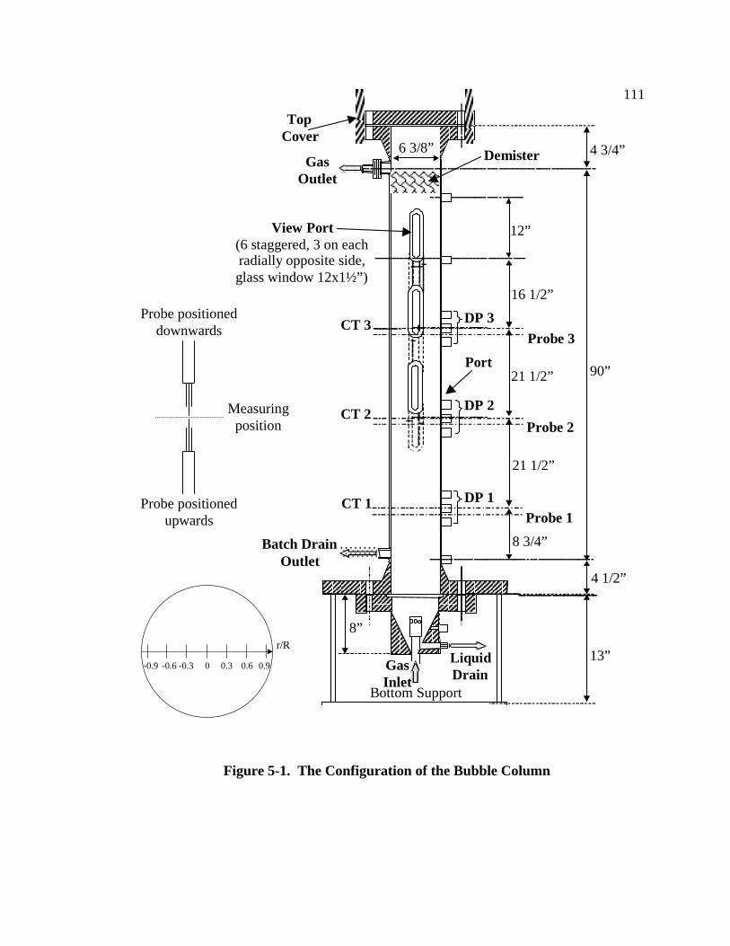
111

21 1/2”

Bottom Support

12”

8 3/4”

21 1/2”

16 1/2”

4 3/4”

90”

4 1/2”

13”

Top Cover

Gas Outlet

Demister

View Port (6 staggered, 3 on each radially opposite side, glass window 12x1½”)

Port

Batch Drain Outlet

Liquid Drain

8”

Gas Inlet

CT 1

CT 2

CT 3

6 3/8”

DP 3

DP 2

DP 1

Probe 2

Probe 1

Probe 3

Measuring position

Probe positioned downwards

Probe positioned upwards

r/R

-0.9 -0.6 -0.3 0 0.3 0.6 0.9

Figure 5-1. The Configuration of the Bubble Column

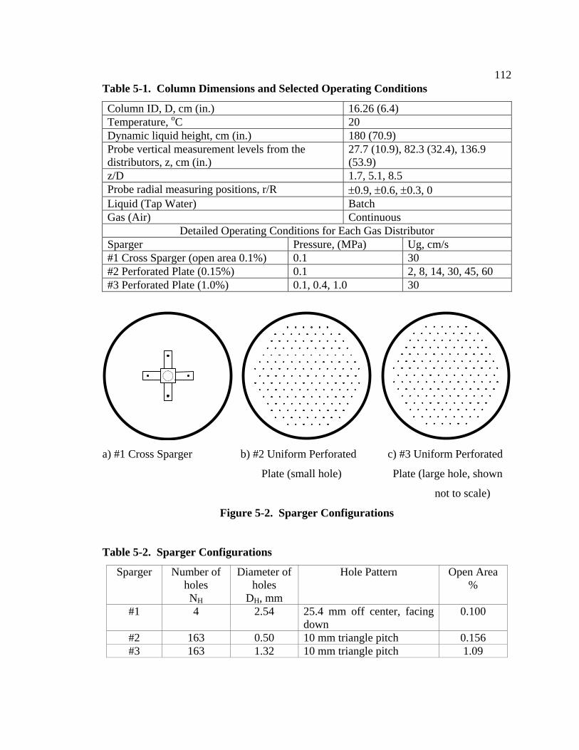
112Table 5-1. Column Dimensions and Selected Operating Conditions

Column ID, D, cm (in.) 16.26 (6.4) Temperature, oC 20 Dynamic liquid height, cm (in.) 180 (70.9) Probe vertical measurement levels from the distributors, z, cm (in.)

27.7 (10.9), 82.3 (32.4), 136.9 (53.9)

z/D 1.7, 5.1, 8.5 Probe radial measuring positions, r/R ±0.9, ±0.6, ±0.3, 0 Liquid (Tap Water) Batch Gas (Air) Continuous

Detailed Operating Conditions for Each Gas Distributor Sparger Pressure, (MPa) Ug, cm/s #1 Cross Sparger (open area 0.1%) 0.1 30 #2 Perforated Plate (0.15%) 0.1 2, 8, 14, 30, 45, 60 #3 Perforated Plate (1.0%) 0.1, 0.4, 1.0 30

a) #1 Cross Sparger b) #2 Uniform Perforated c) #3 Uniform Perforated

Plate (small hole) Plate (large hole, shown

not to scale)

Figure 5-2. Sparger Configurations

Table 5-2. Sparger Configurations

Sparger Number of holes NH

Diameter of holes

DH, mm

Hole Pattern Open Area %

#1 4 2.54 25.4 mm off center, facing down

0.100

#2 163 0.50 10 mm triangle pitch 0.156 #3 163 1.32 10 mm triangle pitch 1.09

113The operating conditions were the same as those used for the CT and CARPT

experiments conducted in CREL (Boon Cheng Ong, 2003). The axial measurement

positions are a little different from those in the CT experiments (z/D= 2.1, 5.5, 9.0)

because the optical probe must employ the fixed ports on the column wall, while the CT

can be positioned freely anywhere along the axial direction. The operating principle of

the four-point probe, discussed earlier, ensures that it accurately measures bubbles

moving upwards when it is positioned downwards, and vice versa. Visual observation

indicates that many bubbles move downwards in bubble columns in transition flow and

churn-turbulent flow, especially in the wall zone. Hence, the four-point probe was

positioned in two directions at each measuring site, i.e., upwards and downwards, and the

probe tip was positioned at the same point when the probe was positioned upwards or

downwards (Figure 5-1). In this way both bubbles moving upwards and those moving

downwards can be measured, instead of only bubbles moving upwards as done in most

other studies involving probes.

5.2 Comparison of the Gas Holdup Profile Obtained by Probe and by CT

The radial profiles of local gas holdup obtained by CT (data of Boon Cheng Ong, 2003, is

used) and by the four-point optical probe were compared. If the gas holdup profile

obtained by the two techniques matched well, and the integrated cross-sectional gas

holdup matched the overall gas holdup obtained by the bed expansion height method

within reasonable error, then one could claim that both the gas holdup profile obtained by

CT and by the four-point optical probe method are reliable.

Figure 5-3 displays an example of the comparison of mean gas holdup radial profiles

obtained by CT and the four-point optical probe at atmospheric pressure. Detailed results

can be found in Appendix D. The value of the gas holdup obtained by the probe shown in

Figures 5-3 and 5-4 is the mean of the values at the symmetric radial positions in the

column along the single chord, i.e. for r/R=0.3 the gas holdup is the mean of the values

obtained at r/R=±0.3. It can be seen that at atmospheric pressure the results of CT and the

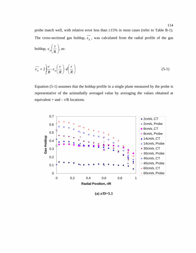
114probe match well, with relative error less than ±15% in most cases (refer to Table B-1).

The cross-sectional gas holdup, gε , was calculated from the radial profile of the gas

holdup, ⎟⎠⎞

⎜⎝⎛ε

Rr

g , as:

∫ ⎟⎠⎞

⎜⎝⎛⋅⎟

⎠⎞

⎜⎝⎛⋅=

1

0

2Rrd

Rr

Rr

gg εε (5-1)

Equation (5-1) assumes that the holdup profile in a single plane measured by the probe is

representative of the azimuthally averaged value by averaging the values obtained at

equivalent + and – r/R locations.

0

0.1

0.2

0.3

0.4

0.5

0.6

0.7

0 0.2 0.4 0.6 0.8 1

Radial Position, r/R

Gas

Hol

dup

2cm/s, CT2cm/s, Probe8cm/s, CT8cm/s, Probe14cm/s, CT14cm/s, Probe30cm/s, CT30cm/s, Probe45cm/s, CT45cm/s, Probe60cm/s, CT60cm/s, Probe

(a) z/D=5.1

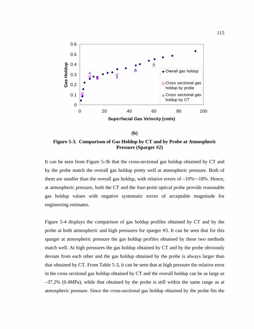
115

0

0.1

0.2

0.3

0.4

0.5

0.6

0 20 40 60 80 1

Superfacial Gas Velocity (cm/s)

Gas

Hol

dup

00

Overall gas holdup

Cross sectional gasholdup by probe

Cross sectional gasholdup by CT

(b)

Figure 5-3. Comparison of Gas Holdup by CT and by Probe at Atmospheric Pressure (Sparger #2)

It can be seen from Figure 5-3b that the cross-sectional gas holdup obtained by CT and

by the probe match the overall gas holdup pretty well at atmospheric pressure. Both of

them are smaller than the overall gas holdup, with relative errors of –10%~-18%. Hence,

at atmospheric pressure, both the CT and the four-point optical probe provide reasonable

gas holdup values with negative systematic errors of acceptable magnitude for

engineering estimates.

Figure 5-4 displays the comparison of gas holdup profiles obtained by CT and by the

probe at both atmospheric and high pressures for sparger #3. It can be seen that for this

sparger at atmospheric pressure the gas holdup profiles obtained by these two methods

match well. At high pressures the gas holdup obtained by CT and by the probe obviously

deviate from each other and the gas holdup obtained by the probe is always larger than

that obtained by CT. From Table 5-3, it can be seen that at high pressure the relative error

in the cross sectional gas holdup obtained by CT and the overall holdup can be as large as

–37.2% (0.4MPa), while that obtained by the probe is still within the same range as at

atmospheric pressure. Since the cross-sectional gas holdup obtained by the probe fits the

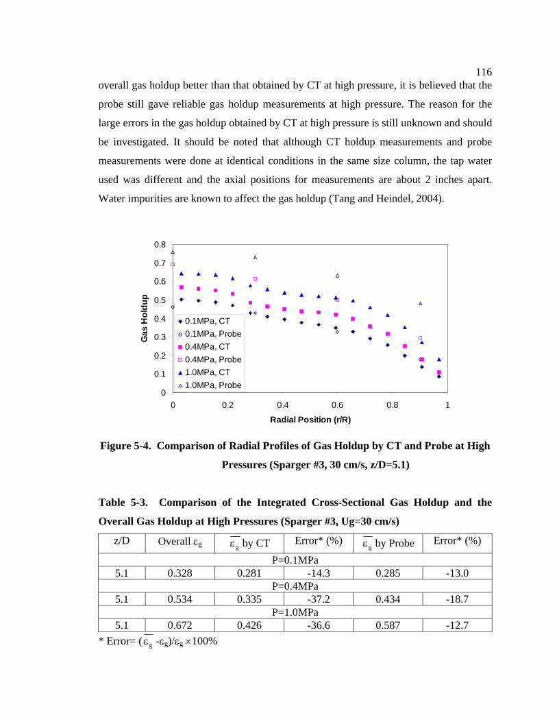
116overall gas holdup better than that obtained by CT at high pressure, it is believed that the

probe still gave reliable gas holdup measurements at high pressure. The reason for the

large errors in the gas holdup obtained by CT at high pressure is still unknown and should

be investigated. It should be noted that although CT holdup measurements and probe

measurements were done at identical conditions in the same size column, the tap water

used was different and the axial positions for measurements are about 2 inches apart.

Water impurities are known to affect the gas holdup (Tang and Heindel, 2004).

0

0.1

0.2

0.3

0.4

0.5

0.6

0.7

0.8

0 0.2 0.4 0.6 0.8 1

Radial Position (r/R)

Gas

Hol

dup

0.1MPa, CT0.1MPa, Probe0.4MPa, CT0.4MPa, Probe1.0MPa, CT1.0MPa, Probe

Figure 5-4. Comparison of Radial Profiles of Gas Holdup by CT and Probe at High

Pressures (Sparger #3, 30 cm/s, z/D=5.1)

Table 5-3. Comparison of the Integrated Cross-Sectional Gas Holdup and the

Overall Gas Holdup at High Pressures (Sparger #3, Ug=30 cm/s)

z/D Overall εg gε by CT Error* (%) gε by Probe Error* (%)

P=0.1MPa 5.1 0.328 0.281 -14.3 0.285 -13.0

P=0.4MPa 5.1 0.534 0.335 -37.2 0.434 -18.7

P=1.0MPa 5.1 0.672 0.426 -36.6 0.587 -12.7

* Error= ( gε -εg)/εg ×100%

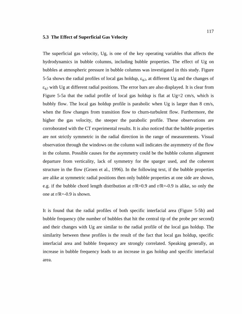
1175.3 The Effect of Superficial Gas Velocity

The superficial gas velocity, Ug, is one of the key operating variables that affects the

hydrodynamics in bubble columns, including bubble properties. The effect of Ug on

bubbles at atmospheric pressure in bubble columns was investigated in this study. Figure

5-5a shows the radial profiles of local gas holdup, εg,l, at different Ug and the changes of

εg,l with Ug at different radial positions. The error bars are also displayed. It is clear from

Figure 5-5a that the radial profile of local gas holdup is flat at Ug=2 cm/s, which is

bubbly flow. The local gas holdup profile is parabolic when Ug is larger than 8 cm/s,

when the flow changes from transition flow to churn-turbulent flow. Furthermore, the

higher the gas velocity, the steeper the parabolic profile. These observations are

corroborated with the CT experimental results. It is also noticed that the bubble properties

are not strictly symmetric in the radial direction in the range of measurements. Visual

observation through the windows on the column wall indicates the asymmetry of the flow

in the column. Possible causes for the asymmetry could be the bubble column alignment

departure from verticality, lack of symmetry for the sparger used, and the coherent

structure in the flow (Groen et al., 1996). In the following text, if the bubble properties

are alike at symmetric radial positions then only bubble properties at one side are shown,

e.g. if the bubble chord length distribution at r/R=0.9 and r/R=-0.9 is alike, so only the

one at r/R=-0.9 is shown.

It is found that the radial profiles of both specific interfacial area (Figure 5-5b) and

bubble frequency (the number of bubbles that hit the central tip of the probe per second)

and their changes with Ug are similar to the radial profile of the local gas holdup. The

similarity between these profiles is the result of the fact that local gas holdup, specific

interfacial area and bubble frequency are strongly correlated. Speaking generally, an

increase in bubble frequency leads to an increase in gas holdup and specific interfacial

area.

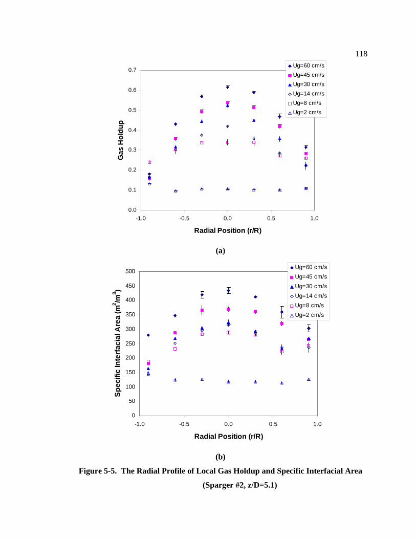
118

0.0

0.1

0.2

0.3

0.4

0.5

0.6

0.7

-1.0 -0.5 0.0 0.5 1.0


Gas

Hol

dup

Ug=60 cm/sUg=45 cm/sUg=30 cm/sUg=14 cm/sUg=8 cm/sUg=2 cm/s

(a)

0

50

100

150

200

250

300

350

400

450

500

-1.0 -0.5 0.0 0.5 1.0


Spec

ific

Inte

rfaci

al A

rea

(m2 /m

3 )


(b)

Figure 5-5. The Radial Profile of Local Gas Holdup and Specific Interfacial Area

(Sparger #2, z/D=5.1)

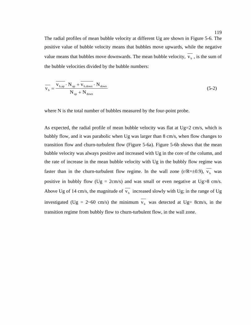
119The radial profiles of mean bubble velocity at different Ug are shown in Figure 5-6. The

positive value of bubble velocity means that bubbles move upwards, while the negative

value means that bubbles move downwards. The mean bubble velocity, bv , is the sum of

the bubble velocities divided by the bubble numbers:

downup

downdown,bupup,bb NN

NvNvv

+

⋅+⋅= (5-2)

where N is the total number of bubbles measured by the four-point probe.

As expected, the radial profile of mean bubble velocity was flat at Ug=2 cm/s, which is

bubbly flow, and it was parabolic when Ug was larger than 8 cm/s, when flow changes to

transition flow and churn-turbulent flow (Figure 5-6a). Figure 5-6b shows that the mean

bubble velocity was always positive and increased with Ug in the core of the column, and

the rate of increase in the mean bubble velocity with Ug in the bubbly flow regime was

faster than in the churn-turbulent flow regime. In the wall zone (r/R=±0.9), bv was

positive in bubbly flow (Ug = 2cm/s) and was small or even negative at Ug>8 cm/s.

Above Ug of 14 cm/s, the magnitude of bv increased slowly with Ug; in the range of Ug

investigated (Ug = 2~60 cm/s) the minimum bv was detected at Ug= 8cm/s, in the

transition regime from bubbly flow to churn-turbulent flow, in the wall zone.

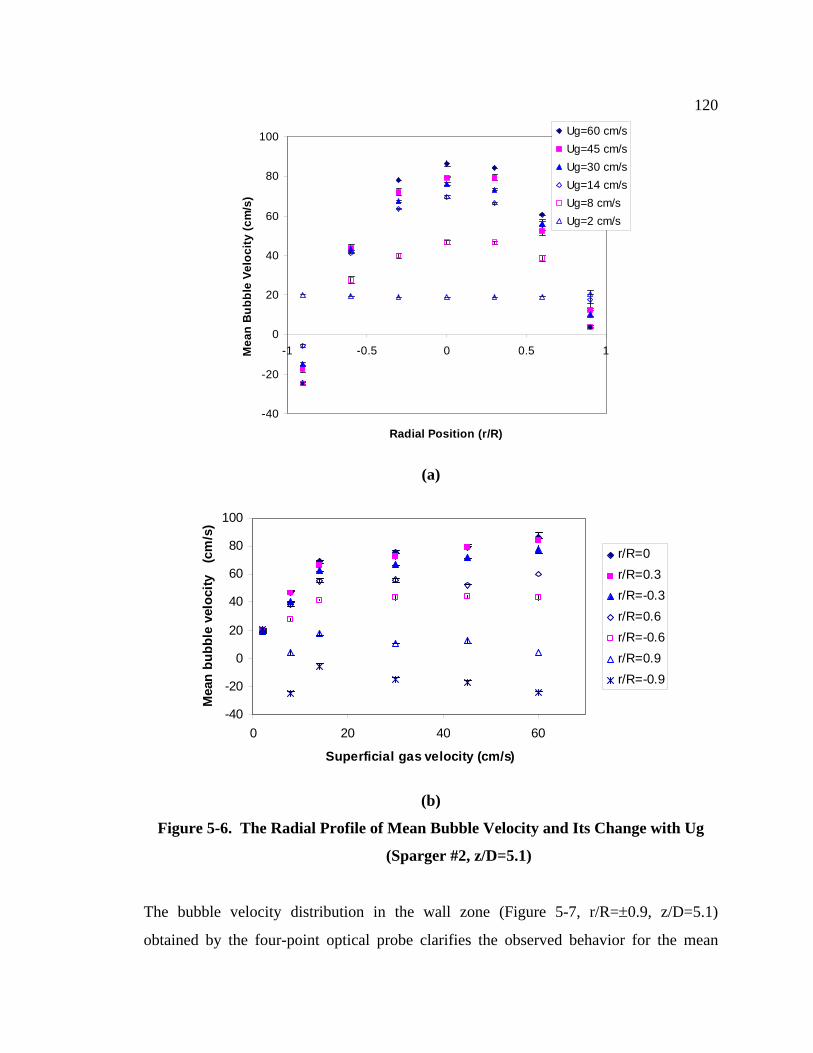
120

-40

-20

0

20

40

60

80

100

-1 -0.5 0 0.5 1


Mea

n B

ubbl

e Ve

loci

ty (c

m/s

)


(a)

-40

-20

0

20

40

60

80

100

0 20 40 60

Superficial gas velocity (cm/s)

Mea

n bu

bble

vel

ocity

(c

m/s

)

r/R=0r/R=0.3r/R=-0.3r/R=0.6r/R=-0.6r/R=0.9r/R=-0.9

(b)

Figure 5-6. The Radial Profile of Mean Bubble Velocity and Its Change with Ug


The bubble velocity distribution in the wall zone (Figure 5-7, r/R=±0.9, z/D=5.1)

obtained by the four-point optical probe clarifies the observed behavior for the mean

121bubble velocity, bv . It should be noted that a large portion of bubbles of very low

velocity cannot be measured by the probe. This is because it takes relatively long time for

very slow bubbles to pass through the four tips of the probe. During this time interval if

the flow field around the bubble changes, the bubble velocity also changes during its

passage by the probe since bubbles move with liquid flow. In this case the velocity of the

bubble determined by the four-point probe is a mean of the early slow velocity and the

later high velocity. Hence, the four-point probe tends to underestimate the probability of

bubbles of very low velocity. However, it should be noted that this bias is usually not

significant because the vertical distance between the central tip and the other tips of the

probe is about 2 mm, if the time scale of the flow field change is 0.1 s, then only bubbles

with velocity lower than about 2 cm/s will be affected. Usually the percentage of bubbles

with velocity as low as this is very low. The bias happens both for bubbles that move

upwards and downwards, so the mean bubble velocity is not affected much by this bias.

At Ug=2 cm/s all bubbles moved upwards (Figure 5-7a), and the peak in the bubble

velocity distribution was thin and sharp. At Ug>8 cm/s, the bubble velocity distributions

at r/R=-0.9 and r/R=0.9 were different. At r/R=-0.9, more bubbles moved downwards

than upwards. At r/R=0.9, almost as many bubbles moved upwards as downwards. As a

result, the radial profile of the mean bubble velocity was not symmetric at z/D=5.1 and

the mean bubble velocity at r/R=-0.9 was smaller than that at r/R=0.9 (Figure 5-6a).

When Ug increased from 8 cm/s to 14 cm/s (i.e., in the transition flow regime) the mean

velocity of bubbles moving upwards increased greatly (from 9.45 to 20.9cm/s at r/R=-0.9

and from 12.4 to 28.3cm/s at r/R=0.9) while that of bubbles moving downwards

increased mildly in magnitude (from –33.8 to -39.1cm/s at r/R=-0.9 and –28.2 to -

34.6cm/s at r/R=0.9). This is because large bubbles, which have high velocity, arose in

the transition flow regime (this is evident from an increase in the number of bubbles of

high velocity in the bubble velocity distributions at Ug=8 cm/s and 14 cm/s, Figures 5-8b

and 5-8c) and assembled in the central stream of the column. The velocity of bubbles

moving downwards in the wall zone increased mainly due to the enhancement of the

liquid recirculation caused by the appearance of large bubbles in the central stream.

Hence, the velocity of bubbles moving upwards jumped and of bubbles moving

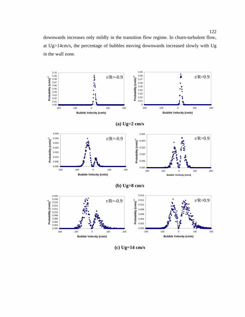
122downwards increases only mildly in the transition flow regime. In churn-turbulent flow,

at Ug>14cm/s, the percentage of bubbles moving downwards increased slowly with Ug

in the wall zone.

0.000.010.020.030.040.050.060.070.080.090.10

-200 -100 0 100 200

Bubble Velocity (cm/s)

Prob

abili

ty (c

m/s

)-1

00.010.020.030.040.050.060.070.080.09

-200 -100 0 100 200


Prob

abili

ty (c

m/s

)-1

r/R=0.9 r/R=-0.9

(a) Ug=2 cm/s

0.000

0.005

0.010

0.015

0.020

0.025

0.030

0.035

-200 -100 0 100 200


Prob

abili

ty (c

m/s

)-1

0.000

0.005

0.010

0.015

0.020

0.025

-200 -100 0 100 200


Prob

abili

ty (c

m/s

)-1

r/R=0.9r/R=-0.9

(b) Ug=8 cm/s

0.0000.0020.0040.0060.0080.0100.0120.0140.0160.0180.020

-200 -100 0 100 200


Prob

abili

ty (c

m/s

)-1

0.000

0.002

0.004

0.006

0.008

0.010

0.012

0.014

-200 -100 0 100 200


Prob

abili

ty (c

m/s

)-1

r/R=0.9r/R=-0.9

(c) Ug=14 cm/s

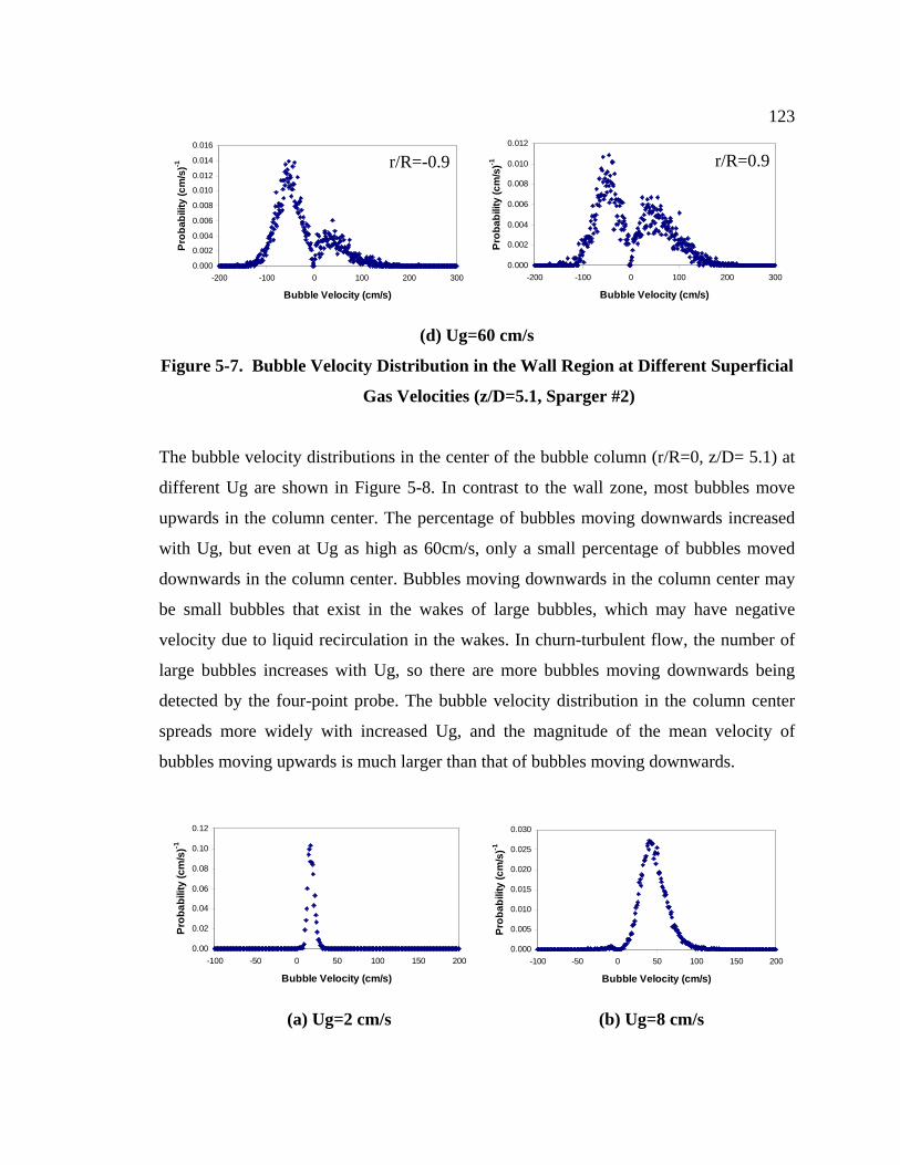
123

0.000

0.002

0.004

0.006

0.008

0.010

0.012

0.014

0.016

-200 -100 0 100 200 300


Prob

abili

ty (c

m/s

)-1

0.000

0.002

0.004

0.006

0.008

0.010

0.012

-200 -100 0 100 200 300


Prob

abili

ty (c

m/s

)-1

r/R=0.9 r/R=-0.9

(d) Ug=60 cm/s

Figure 5-7. Bubble Velocity Distribution in the Wall Region at Different Superficial

Gas Velocities (z/D=5.1, Sparger #2)

The bubble velocity distributions in the center of the bubble column (r/R=0, z/D= 5.1) at

different Ug are shown in Figure 5-8. In contrast to the wall zone, most bubbles move

upwards in the column center. The percentage of bubbles moving downwards increased

with Ug, but even at Ug as high as 60cm/s, only a small percentage of bubbles moved

downwards in the column center. Bubbles moving downwards in the column center may

be small bubbles that exist in the wakes of large bubbles, which may have negative

velocity due to liquid recirculation in the wakes. In churn-turbulent flow, the number of

large bubbles increases with Ug, so there are more bubbles moving downwards being

detected by the four-point probe. The bubble velocity distribution in the column center

spreads more widely with increased Ug, and the magnitude of the mean velocity of

bubbles moving upwards is much larger than that of bubbles moving downwards.

0.00

0.02

0.04

0.06

0.08

0.10

0.12

-100 -50 0 50 100 150 200


Prob

abili

ty (c

m/s

)-1

0.000

0.005

0.010

0.015

0.020

0.025

0.030

-100 -50 0 50 100 150 200


Prob

abili

ty (c

m/s

)-1

(a) Ug=2 cm/s (b) Ug=8 cm/s

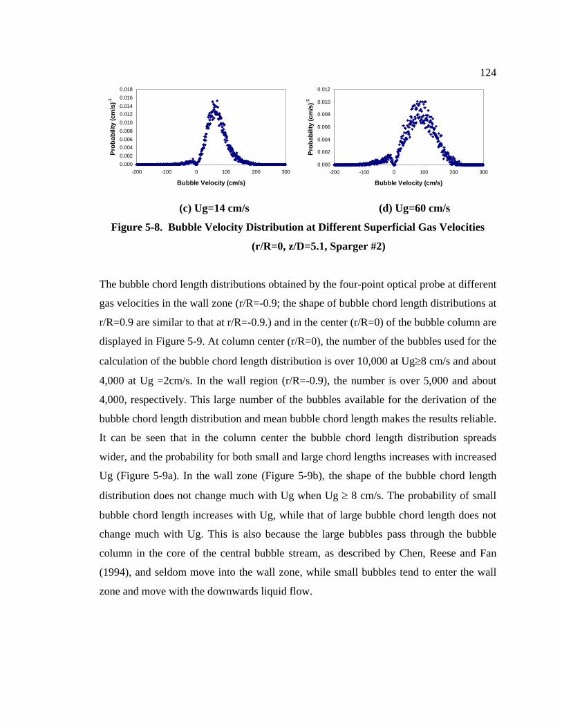
124

0.0000.0020.0040.0060.0080.0100.0120.0140.0160.018

-200 -100 0 100 200 300


Prob

abili

ty (c

m/s

)-1

0.000

0.002

0.004

0.006

0.008

0.010

0.012

-200 -100 0 100 200 300


Prob

abili

ty (c

m/s

)-1

(c) Ug=14 cm/s (d) Ug=60 cm/s

Figure 5-8. Bubble Velocity Distribution at Different Superficial Gas Velocities

(r/R=0, z/D=5.1, Sparger #2)

The bubble chord length distributions obtained by the four-point optical probe at different

gas velocities in the wall zone (r/R=-0.9; the shape of bubble chord length distributions at

r/R=0.9 are similar to that at r/R=-0.9.) and in the center (r/R=0) of the bubble column are

displayed in Figure 5-9. At column center (r/R=0), the number of the bubbles used for the

calculation of the bubble chord length distribution is over 10,000 at Ug≥8 cm/s and about

4,000 at Ug =2cm/s. In the wall region (r/R=-0.9), the number is over 5,000 and about

4,000, respectively. This large number of the bubbles available for the derivation of the

bubble chord length distribution and mean bubble chord length makes the results reliable.

It can be seen that in the column center the bubble chord length distribution spreads

wider, and the probability for both small and large chord lengths increases with increased

Ug (Figure 5-9a). In the wall zone (Figure 5-9b), the shape of the bubble chord length

distribution does not change much with Ug when Ug ≥ 8 cm/s. The probability of small

bubble chord length increases with Ug, while that of large bubble chord length does not

change much with Ug. This is also because the large bubbles pass through the bubble

column in the core of the central bubble stream, as described by Chen, Reese and Fan

(1994), and seldom move into the wall zone, while small bubbles tend to enter the wall

zone and move with the downwards liquid flow.

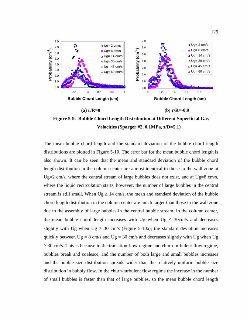
125

0.0

1.0

2.0

3.0

4.0

5.0

6.0

7.0

8.0

0 0.2 0.4 0.6 0.8 1

Bubble Chord Length (cm)

Prob

abili

ty (c

m-1

)Ug= 2 cm/sUg= 8 cm/sUg= 14 cm/sUg= 30 cm/sUg= 45 cm/sUg= 60 cm/s

0.0

1.0

2.0

3.0

4.0

5.0

6.0

7.0

0 0.2 0.4 0.6 0.8 1


Prob

abili

ty (c

m-1

)

Ug= 2 cm/sUg= 8 cm/sUg= 14 cm/sUg= 30 cm/sUg= 45 cm/sUg= 60 cm/s

(a) r/R=0 (b) r/R=-0.9

Figure 5-9. Bubble Chord Length Distribution at Different Superficial Gas

Velocities (Sparger #2, 0.1MPa, z/D=5.1)

The mean bubble chord length and the standard deviation of the bubble chord length

distributions are plotted in Figure 5-10. The error bar for the mean bubble chord length is

also shown. It can be seen that the mean and standard deviation of the bubble chord

length distribution in the column center are almost identical to those in the wall zone at

Ug=2 cm/s, where the central stream of large bubbles does not exist, and at Ug=8 cm/s,

where the liquid recirculation starts, however, the number of large bubbles in the central

stream is still small. When Ug ≥ 14 cm/s, the mean and standard deviation of the bubble

chord length distribution in the column center are much larger than those in the wall zone

due to the assembly of large bubbles in the central bubble stream. In the column center,

the mean bubble chord length increases with Ug when Ug ≤ 30cm/s and decreases

slightly with Ug when Ug ≥ 30 cm/s (Figure 5-10a); the standard deviation increases

quickly between Ug = 8 cm/s and Ug = 30 cm/s and decreases slightly with Ug when Ug

≥ 30 cm/s. This is because in the transition flow regime and churn-turbulent flow regime,

bubbles break and coalesce, and the number of both large and small bubbles increases

and the bubble size distribution spreads wider than the relatively uniform bubble size

distribution in bubbly flow. In the churn-turbulent flow regime the increase in the number

of small bubbles is faster than that of large bubbles, so the mean bubble chord length

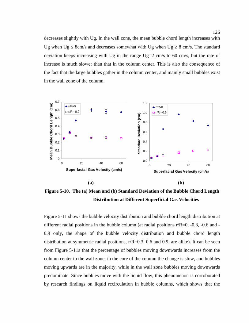
126decreases slightly with Ug. In the wall zone, the mean bubble chord length increases with

Ug when Ug ≤ 8cm/s and decreases somewhat with Ug when Ug ≥ 8 cm/s. The standard

deviation keeps increasing with Ug in the range Ug=2 cm/s to 60 cm/s, but the rate of

increase is much slower than that in the column center. This is also the consequence of

the fact that the large bubbles gather in the column center, and mainly small bubbles exist

in the wall zone of the column.

0

0.1

0.2

0.3

0.4

0.5

0.6

0.7

0 20 40 60


Mea

n B

ubbl

e C

hord

Len

gth

(cm

)

r/R=0

r/R=-0.9

0.0

0.2

0.4

0.6

0.8

1.0

1.2

0 20 40 60


Stan

dard

Dev

iatio

n (c

m)

r/R=0

r/R=-0.9

(a) (b)

Figure 5-10. The (a) Mean and (b) Standard Deviation of the Bubble Chord Length

Distribution at Different Superficial Gas Velocities

Figure 5-11 shows the bubble velocity distribution and bubble chord length distribution at

different radial positions in the bubble column (at radial positions r/R=0, -0.3, -0.6 and -

0.9 only, the shape of the bubble velocity distribution and bubble chord length

distribution at symmetric radial positions, r/R=0.3, 0.6 and 0.9, are alike). It can be seen

from Figure 5-11a that the percentage of bubbles moving downwards increases from the

column center to the wall zone; in the core of the column the change is slow, and bubbles

moving upwards are in the majority, while in the wall zone bubbles moving downwards

predominate. Since bubbles move with the liquid flow, this phenomenon is corroborated

by research findings on liquid recirculation in bubble columns, which shows that the

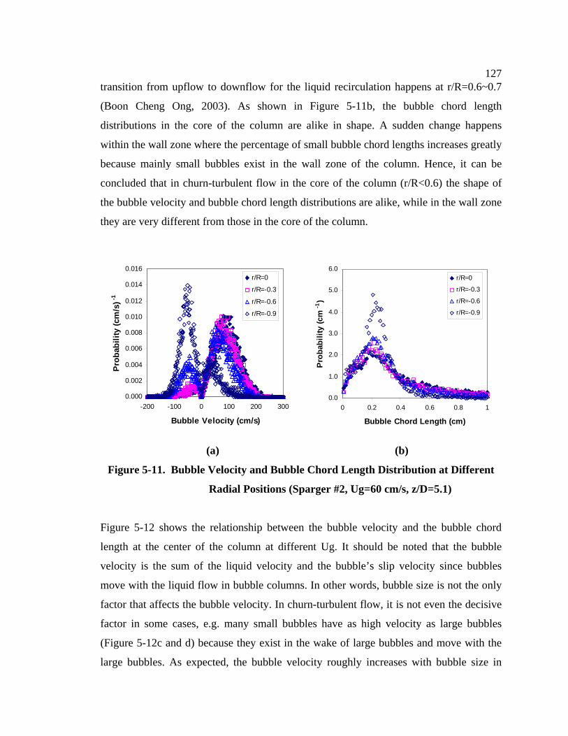
127transition from upflow to downflow for the liquid recirculation happens at r/R=0.6~0.7

(Boon Cheng Ong, 2003). As shown in Figure 5-11b, the bubble chord length

distributions in the core of the column are alike in shape. A sudden change happens

within the wall zone where the percentage of small bubble chord lengths increases greatly

because mainly small bubbles exist in the wall zone of the column. Hence, it can be

concluded that in churn-turbulent flow in the core of the column (r/R<0.6) the shape of

the bubble velocity and bubble chord length distributions are alike, while in the wall zone

they are very different from those in the core of the column.

0.000

0.002

0.004

0.006

0.008

0.010

0.012

0.014

0.016

-200 -100 0 100 200 300


Pro

babi

lity

(cm

/s)-1

r/R=0

r/R=-0.3

r/R=-0.6

r/R=-0.9

0.0

1.0

2.0

3.0

4.0

5.0

6.0

0 0.2 0.4 0.6 0.8 1


Pro

babi

lity

(cm

-1)

r/R=0

r/R=-0.3

r/R=-0.6

r/R=-0.9

(a) (b)

Figure 5-11. Bubble Velocity and Bubble Chord Length Distribution at Different

Radial Positions (Sparger #2, Ug=60 cm/s, z/D=5.1)

Figure 5-12 shows the relationship between the bubble velocity and the bubble chord

length at the center of the column at different Ug. It should be noted that the bubble

velocity is the sum of the liquid velocity and the bubble’s slip velocity since bubbles

move with the liquid flow in bubble columns. In other words, bubble size is not the only

factor that affects the bubble velocity. In churn-turbulent flow, it is not even the decisive

factor in some cases, e.g. many small bubbles have as high velocity as large bubbles

(Figure 5-12c and d) because they exist in the wake of large bubbles and move with the

large bubbles. As expected, the bubble velocity roughly increases with bubble size in

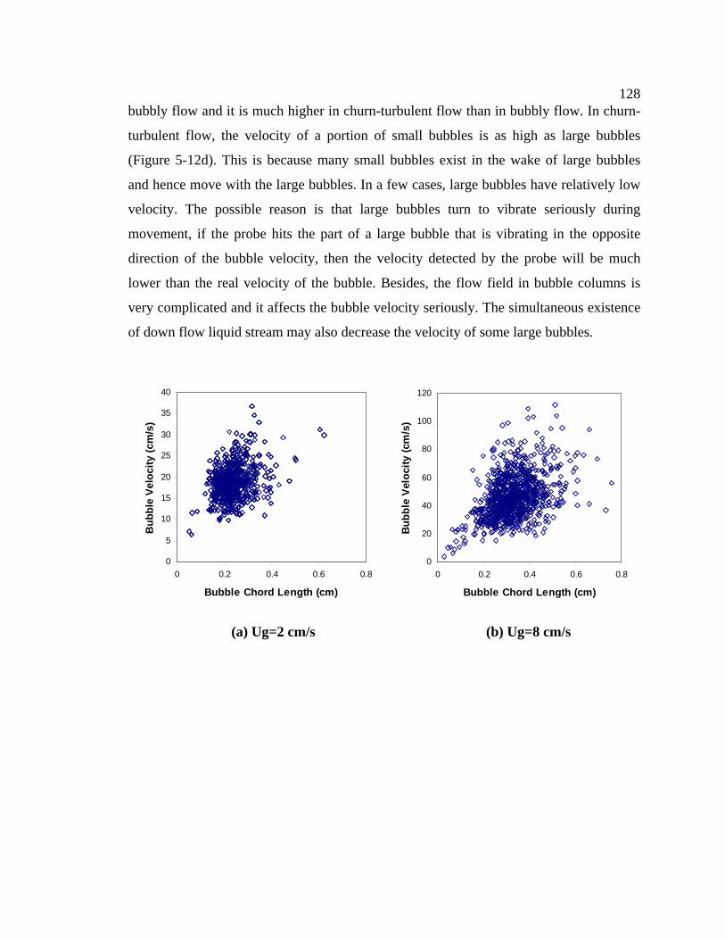
128bubbly flow and it is much higher in churn-turbulent flow than in bubbly flow. In churn-

turbulent flow, the velocity of a portion of small bubbles is as high as large bubbles

(Figure 5-12d). This is because many small bubbles exist in the wake of large bubbles

and hence move with the large bubbles. In a few cases, large bubbles have relatively low

velocity. The possible reason is that large bubbles turn to vibrate seriously during

movement, if the probe hits the part of a large bubble that is vibrating in the opposite

direction of the bubble velocity, then the velocity detected by the probe will be much

lower than the real velocity of the bubble. Besides, the flow field in bubble columns is

very complicated and it affects the bubble velocity seriously. The simultaneous existence

of down flow liquid stream may also decrease the velocity of some large bubbles.

0

5

10

15

20

25

30

35

40

0 0.2 0.4 0.6 0.8


Bub

ble

Velo

city

(cm

/s)

0

20

40

60

80

100

120

0 0.2 0.4 0.6 0.8


Bub

ble

Velo

city

(cm

/s)


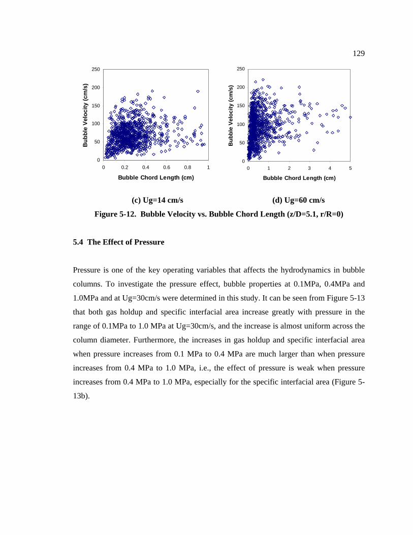
129

0

50

100

150

200

250

0 0.2 0.4 0.6 0.8 1


Bub

ble

Velo

city

(cm

/s)

0

50

100

150

200

250

0 1 2 3 4 5


Bub

ble

Velo

city

(cm

/s)


Figure 5-12. Bubble Velocity vs. Bubble Chord Length (z/D=5.1, r/R=0)

5.4 The Effect of Pressure

Pressure is one of the key operating variables that affects the hydrodynamics in bubble

columns. To investigate the pressure effect, bubble properties at 0.1MPa, 0.4MPa and

1.0MPa and at Ug=30cm/s were determined in this study. It can be seen from Figure 5-13

that both gas holdup and specific interfacial area increase greatly with pressure in the

range of 0.1MPa to 1.0 MPa at Ug=30cm/s, and the increase is almost uniform across the

column diameter. Furthermore, the increases in gas holdup and specific interfacial area

when pressure increases from 0.1 MPa to 0.4 MPa are much larger than when pressure

increases from 0.4 MPa to 1.0 MPa, i.e., the effect of pressure is weak when pressure

increases from 0.4 MPa to 1.0 MPa, especially for the specific interfacial area (Figure 5-

13b).

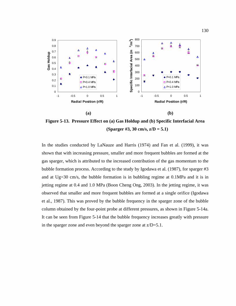
130

0

0.1

0.2

0.3

0.4

0.5

0.6

0.7

0.8

0.9

-1 -0.5 0 0.5 1


Gas

Hol

dup

P=0.1 MPa

P=0.4 MPa

P=1.0 MPa

0

100

200

300

400

500

600

700

800

-1 -0.5 0 0.5 1


Spe

cific

Inte

rfaci

al A

rea

(m2 /m

3 )

P=0.1 MPa

P=0.4 MPa

P=1.0 MPa

(a) (b)

Figure 5-13. Pressure Effect on (a) Gas Holdup and (b) Specific Interfacial Area

(Sparger #3, 30 cm/s, z/D = 5.1)

In the studies conducted by LaNauze and Harris (1974) and Fan et al. (1999), it was

shown that with increasing pressure, smaller and more frequent bubbles are formed at the

gas sparger, which is attributed to the increased contribution of the gas momentum to the

bubble formation process. According to the study by Igodawa et al. (1987), for sparger #3

and at Ug=30 cm/s, the bubble formation is in bubbling regime at 0.1MPa and it is in

jetting regime at 0.4 and 1.0 MPa (Boon Cheng Ong, 2003). In the jetting regime, it was

observed that smaller and more frequent bubbles are formed at a single orifice (Igodawa

et al., 1987). This was proved by the bubble frequency in the sparger zone of the bubble

column obtained by the four-point probe at different pressures, as shown in Figure 5-14a.

It can be seen from Figure 5-14 that the bubble frequency increases greatly with pressure

in the sparger zone and even beyond the sparger zone at z/D=5.1.

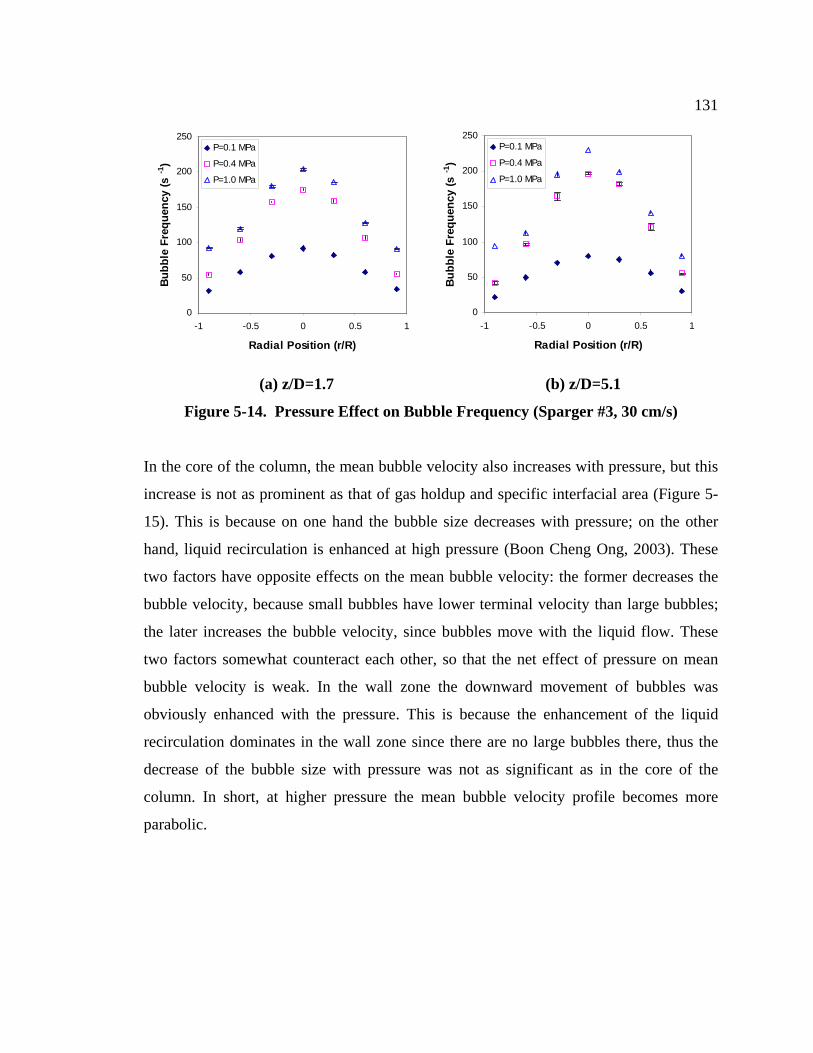
131

0

50

100

150

200

250

-1 -0.5 0 0.5 1


Bubb

le F

requ

ency

(s-1

)P=0.1 MPa

P=0.4 MPa

P=1.0 MPa

0

50

100

150

200

250

-1 -0.5 0 0.5 1


Bub

ble

Freq

uenc

y (s

-1)

P=0.1 MPa

P=0.4 MPa

P=1.0 MPa

(a) z/D=1.7 (b) z/D=5.1

Figure 5-14. Pressure Effect on Bubble Frequency (Sparger #3, 30 cm/s)

In the core of the column, the mean bubble velocity also increases with pressure, but this

increase is not as prominent as that of gas holdup and specific interfacial area (Figure 5-

15). This is because on one hand the bubble size decreases with pressure; on the other

hand, liquid recirculation is enhanced at high pressure (Boon Cheng Ong, 2003). These

two factors have opposite effects on the mean bubble velocity: the former decreases the

bubble velocity, because small bubbles have lower terminal velocity than large bubbles;

the later increases the bubble velocity, since bubbles move with the liquid flow. These

two factors somewhat counteract each other, so that the net effect of pressure on mean

bubble velocity is weak. In the wall zone the downward movement of bubbles was

obviously enhanced with the pressure. This is because the enhancement of the liquid

recirculation dominates in the wall zone since there are no large bubbles there, thus the

decrease of the bubble size with pressure was not as significant as in the core of the

column. In short, at higher pressure the mean bubble velocity profile becomes more

parabolic.

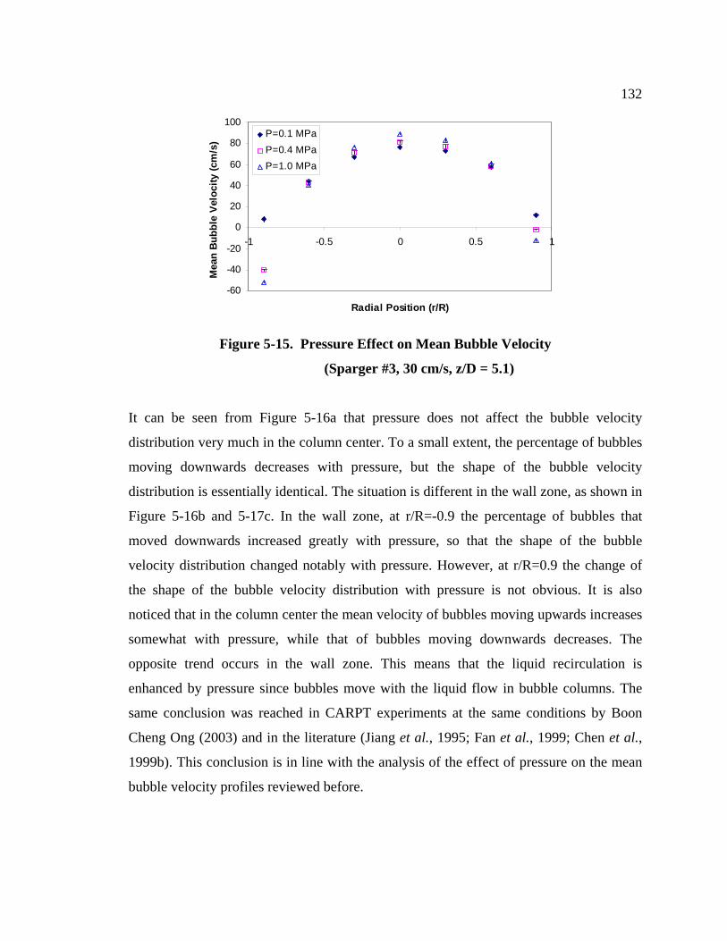
132

-60

-40

-20

0

20

40

60

80

100

-1 -0.5 0 0.5 1


Mea

n B

ubbl

e Ve

loci

ty (c

m/s

)

P=0.1 MPaP=0.4 MPaP=1.0 MPa

Figure 5-15. Pressure Effect on Mean Bubble Velocity

(Sparger #3, 30 cm/s, z/D = 5.1)

It can be seen from Figure 5-16a that pressure does not affect the bubble velocity

distribution very much in the column center. To a small extent, the percentage of bubbles

moving downwards decreases with pressure, but the shape of the bubble velocity

distribution is essentially identical. The situation is different in the wall zone, as shown in

Figure 5-16b and 5-17c. In the wall zone, at r/R=-0.9 the percentage of bubbles that

moved downwards increased greatly with pressure, so that the shape of the bubble

velocity distribution changed notably with pressure. However, at r/R=0.9 the change of

the shape of the bubble velocity distribution with pressure is not obvious. It is also

noticed that in the column center the mean velocity of bubbles moving upwards increases

somewhat with pressure, while that of bubbles moving downwards decreases. The

opposite trend occurs in the wall zone. This means that the liquid recirculation is

enhanced by pressure since bubbles move with the liquid flow in bubble columns. The

same conclusion was reached in CARPT experiments at the same conditions by Boon

Cheng Ong (2003) and in the literature (Jiang et al., 1995; Fan et al., 1999; Chen et al.,

1999b). This conclusion is in line with the analysis of the effect of pressure on the mean

bubble velocity profiles reviewed before.

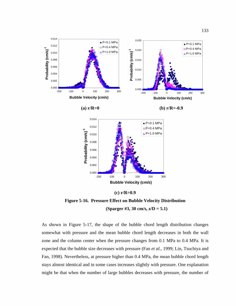
133

0.000

0.002

0.004

0.006

0.008

0.010

0.012

0.014

-200 -100 0 100 200 300


Prob

abili

ty (c

m/s

)-1P=0.1 MPaP=0.4 MPaP=1.0 MPa

0.000

0.005

0.010

0.015

0.020

0.025

-200 -100 0 100 200 300


Prob

abili

ty (c

m/s

)-1


(a) r/R=0 (b) r/R=-0.9

0.000

0.002

0.004

0.006

0.008

0.010

0.012

0.014

-200 -100 0 100 200 300


Prob

abili

ty (c

m/s

)-1


(c) r/R=0.9

Figure 5-16. Pressure Effect on Bubble Velocity Distribution

(Sparger #3, 30 cm/s, z/D = 5.1)

As shown in Figure 5-17, the shape of the bubble chord length distribution changes

somewhat with pressure and the mean bubble chord length decreases in both the wall

zone and the column center when the pressure changes from 0.1 MPa to 0.4 MPa. It is

expected that the bubble size decreases with pressure (Fan et al., 1999; Lin, Tsuchiya and

Fan, 1998). Nevertheless, at pressure higher than 0.4 MPa, the mean bubble chord length

stays almost identical and in some cases increases slightly with pressure. One explanation

might be that when the number of large bubbles decreases with pressure, the number of

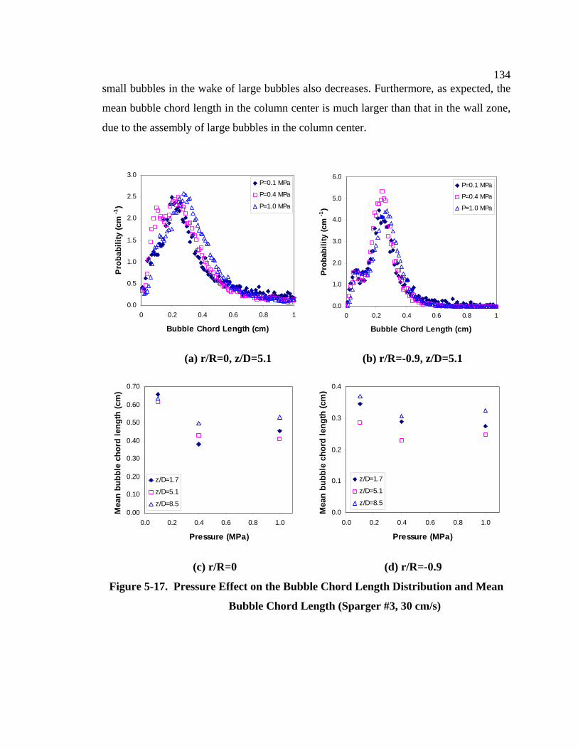
134small bubbles in the wake of large bubbles also decreases. Furthermore, as expected, the

mean bubble chord length in the column center is much larger than that in the wall zone,

due to the assembly of large bubbles in the column center.

0.0

0.5

1.0

1.5

2.0

2.5

3.0

0 0.2 0.4 0.6 0.8 1


Pro

babi

lity

(cm

-1)

P=0.1 MPa

P=0.4 MPa

P=1.0 MPa

0.0

1.0

2.0

3.0

4.0

5.0

6.0

0 0.2 0.4 0.6 0.8 1

Bubble Chord Length (cm)Pr

obab

ility

(cm

-1)

P=0.1 MPa

P=0.4 MPa

P=1.0 MPa

(a) r/R=0, z/D=5.1 (b) r/R=-0.9, z/D=5.1

0.00

0.10

0.20

0.30

0.40

0.50

0.60

0.70

0.0 0.2 0.4 0.6 0.8 1.0

Pressure (MPa)

Mea

n bu

bble

cho

rd le

ngth

(cm

)

z/D=1.7

z/D=5.1

z/D=8.5

0.0

0.1

0.2

0.3

0.4

0.0 0.2 0.4 0.6 0.8 1.0

Pressure (MPa)

Mea

n bu

bble

cho

rd le

ngth

(cm

)

z/D=1.7

z/D=5.1

z/D=8.5

(c) r/R=0 (d) r/R=-0.9

Figure 5-17. Pressure Effect on the Bubble Chord Length Distribution and Mean

Bubble Chord Length (Sparger #3, 30 cm/s)

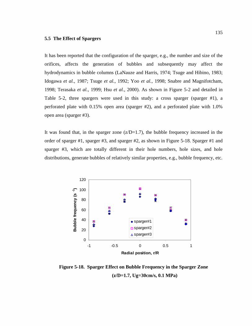
1355.5 The Effect of Spargers

It has been reported that the configuration of the sparger, e.g., the number and size of the

orifices, affects the generation of bubbles and subsequently may affect the

hydrodynamics in bubble columns (LaNauze and Harris, 1974; Tsuge and Hibino, 1983;

Idogawa et al., 1987; Tsuge et al., 1992; Yoo et al., 1998; Snabre and Magnifotcham,

1998; Terasaka et al., 1999; Hsu et al., 2000). As shown in Figure 5-2 and detailed in

Table 5-2, three spargers were used in this study: a cross sparger (sparger #1), a

perforated plate with 0.15% open area (sparger #2), and a perforated plate with 1.0%

open area (sparger #3).

It was found that, in the sparger zone (z/D=1.7), the bubble frequency increased in the

order of sparger #1, sparger #3, and sparger #2, as shown in Figure 5-18. Sparger #1 and

sparger #3, which are totally different in their hole numbers, hole sizes, and hole

distributions, generate bubbles of relatively similar properties, e.g., bubble frequency, etc.

0

20

40

60

80

100

120

-1 -0.5 0 0.5 1

Radial position, r/R

Bub

ble

freq

uenc

y (s

-1)

sparger#1sparger#2sparger#3

Figure 5-18. Sparger Effect on Bubble Frequency in the Sparger Zone

(z/D=1.7, Ug=30cm/s, 0.1 MPa)

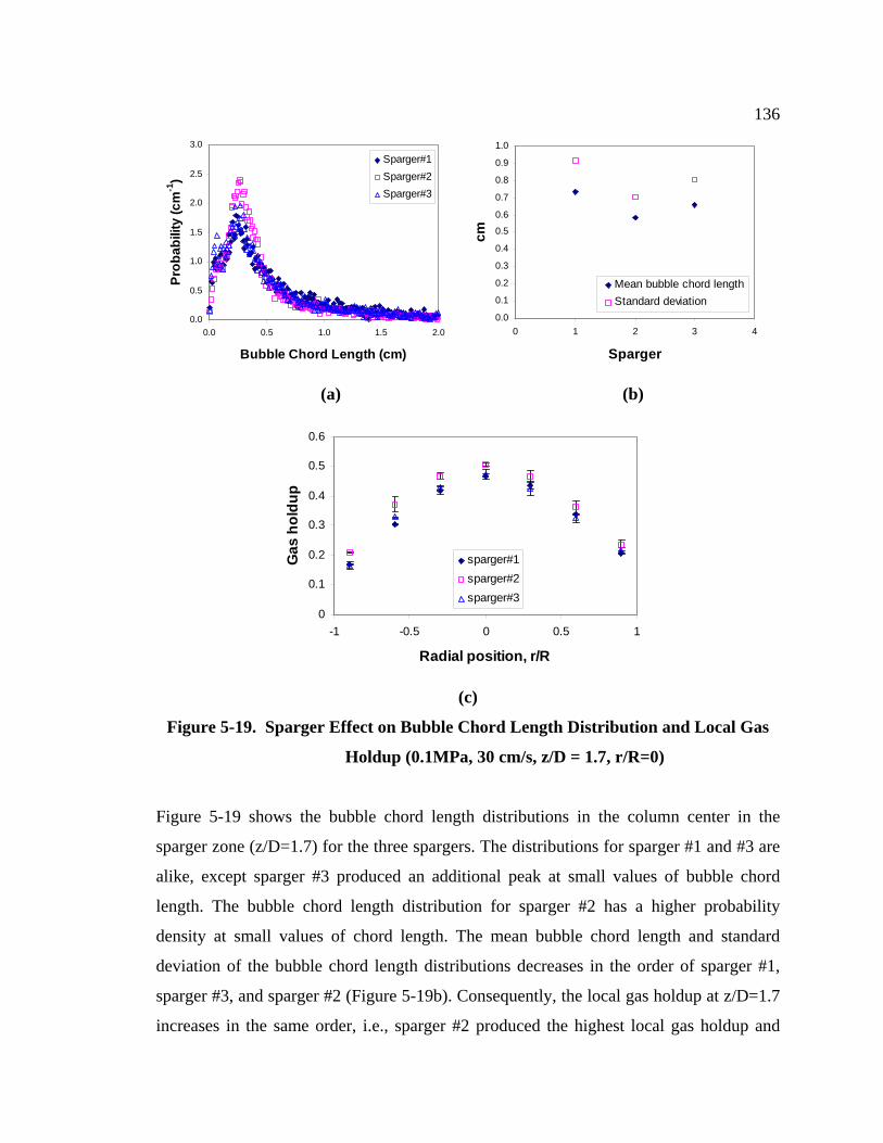
136

0.0

0.5

1.0

1.5

2.0

2.5

3.0

0.0 0.5 1.0 1.5 2.0


Prob

abili

ty (c

m-1

)Sparger#1Sparger#2Sparger#3

0.0

0.1

0.2

0.3

0.4

0.5

0.6

0.7

0.8

0.9

1.0

0 1 2 3 4

Sparger

cm

Mean bubble chord lengthStandard deviation

(a) (b)

0

0.1

0.2

0.3

0.4

0.5

0.6

-1 -0.5 0 0.5 1


Gas

hol

dup


(c)

Figure 5-19. Sparger Effect on Bubble Chord Length Distribution and Local Gas

Holdup (0.1MPa, 30 cm/s, z/D = 1.7, r/R=0)

Figure 5-19 shows the bubble chord length distributions in the column center in the

sparger zone (z/D=1.7) for the three spargers. The distributions for sparger #1 and #3 are

alike, except sparger #3 produced an additional peak at small values of bubble chord

length. The bubble chord length distribution for sparger #2 has a higher probability

density at small values of chord length. The mean bubble chord length and standard

deviation of the bubble chord length distributions decreases in the order of sparger #1,

sparger #3, and sparger #2 (Figure 5-19b). Consequently, the local gas holdup at z/D=1.7

increases in the same order, i.e., sparger #2 produced the highest local gas holdup and

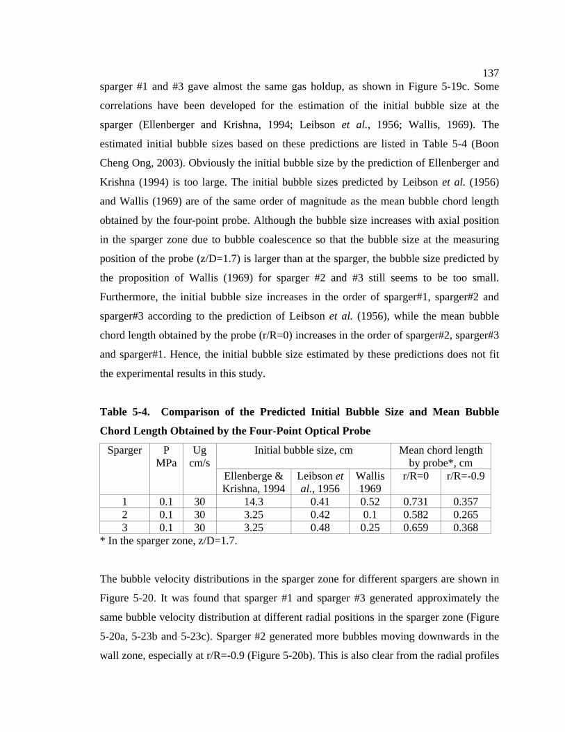
137sparger #1 and #3 gave almost the same gas holdup, as shown in Figure 5-19c. Some

correlations have been developed for the estimation of the initial bubble size at the

sparger (Ellenberger and Krishna, 1994; Leibson et al., 1956; Wallis, 1969). The

estimated initial bubble sizes based on these predictions are listed in Table 5-4 (Boon

Cheng Ong, 2003). Obviously the initial bubble size by the prediction of Ellenberger and

Krishna (1994) is too large. The initial bubble sizes predicted by Leibson et al. (1956)

and Wallis (1969) are of the same order of magnitude as the mean bubble chord length

obtained by the four-point probe. Although the bubble size increases with axial position

in the sparger zone due to bubble coalescence so that the bubble size at the measuring

position of the probe (z/D=1.7) is larger than at the sparger, the bubble size predicted by

the proposition of Wallis (1969) for sparger #2 and #3 still seems to be too small.

Furthermore, the initial bubble size increases in the order of sparger#1, sparger#2 and

sparger#3 according to the prediction of Leibson et al. (1956), while the mean bubble

chord length obtained by the probe (r/R=0) increases in the order of sparger#2, sparger#3

and sparger#1. Hence, the initial bubble size estimated by these predictions does not fit

the experimental results in this study.

Table 5-4. Comparison of the Predicted Initial Bubble Size and Mean Bubble

Chord Length Obtained by the Four-Point Optical Probe

Initial bubble size, cm Mean chord length by probe*, cm

Sparger P MPa

Ug cm/s

Ellenberge & Krishna, 1994

Leibson et al., 1956

Wallis 1969

r/R=0 r/R=-0.9

1 0.1 30 14.3 0.41 0.52 0.731 0.357 2 0.1 30 3.25 0.42 0.1 0.582 0.265 3 0.1 30 3.25 0.48 0.25 0.659 0.368

* In the sparger zone, z/D=1.7.

The bubble velocity distributions in the sparger zone for different spargers are shown in

Figure 5-20. It was found that sparger #1 and sparger #3 generated approximately the

same bubble velocity distribution at different radial positions in the sparger zone (Figure

5-20a, 5-23b and 5-23c). Sparger #2 generated more bubbles moving downwards in the

wall zone, especially at r/R=-0.9 (Figure 5-20b). This is also clear from the radial profiles

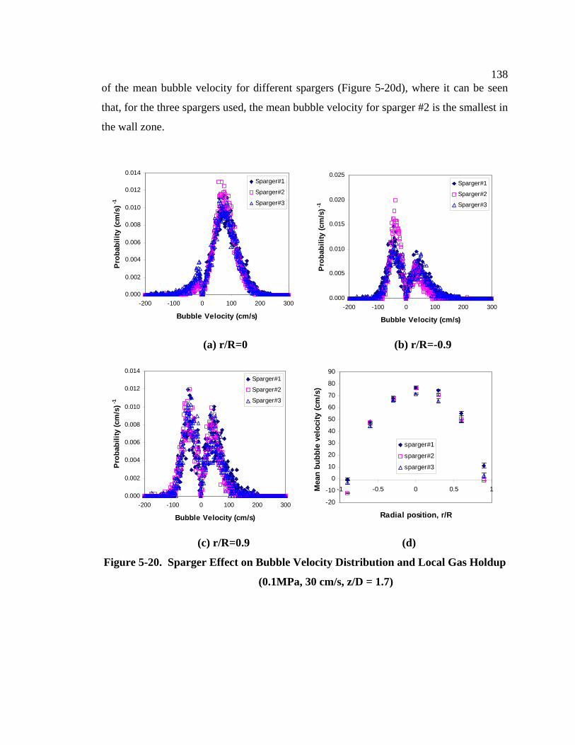
138of the mean bubble velocity for different spargers (Figure 5-20d), where it can be seen

that, for the three spargers used, the mean bubble velocity for sparger #2 is the smallest in

the wall zone.

0.000

0.002

0.004

0.006

0.008

0.010

0.012

0.014

-200 -100 0 100 200 300


Pro

babi

lity

(cm

/s)-1

Sparger#1

Sparger#2

Sparger#3

0.000

0.005

0.010

0.015

0.020

0.025

-200 -100 0 100 200 300

Bubble Velocity (cm/s)Pr

obab

ility

(cm

/s)-1

Sparger#1

Sparger#2

Sparger#3

(a) r/R=0 (b) r/R=-0.9

0.000

0.002

0.004

0.006

0.008

0.010

0.012

0.014

-200 -100 0 100 200 300


Pro

babi

lity

(cm

/s)-1

Sparger#1

Sparger#2

Sparger#3

-20

-10

0

10

20

30

40

50

60

70

80

90

-1 -0.5 0 0.5 1


Mea

n bu

bble

vel

ocity

(cm

/s)

sparger#1

sparger#2

sparger#3

(c) r/R=0.9 (d)

Figure 5-20. Sparger Effect on Bubble Velocity Distribution and Local Gas Holdup

(0.1MPa, 30 cm/s, z/D = 1.7)

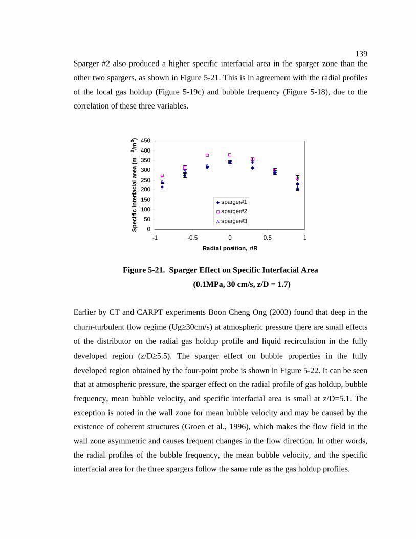
139Sparger #2 also produced a higher specific interfacial area in the sparger zone than the

other two spargers, as shown in Figure 5-21. This is in agreement with the radial profiles

of the local gas holdup (Figure 5-19c) and bubble frequency (Figure 5-18), due to the

correlation of these three variables.

0

50100

150

200250

300

350400

450

-1 -0.5 0 0.5 1


Spec

ific

inte

rfaci

al a

rea

(m2 /m

3 )


Figure 5-21. Sparger Effect on Specific Interfacial Area

(0.1MPa, 30 cm/s, z/D = 1.7)

Earlier by CT and CARPT experiments Boon Cheng Ong (2003) found that deep in the

churn-turbulent flow regime (Ug≥30cm/s) at atmospheric pressure there are small effects

of the distributor on the radial gas holdup profile and liquid recirculation in the fully

developed region (z/D≥5.5). The sparger effect on bubble properties in the fully

developed region obtained by the four-point probe is shown in Figure 5-22. It can be seen

that at atmospheric pressure, the sparger effect on the radial profile of gas holdup, bubble

frequency, mean bubble velocity, and specific interfacial area is small at z/D=5.1. The

exception is noted in the wall zone for mean bubble velocity and may be caused by the

existence of coherent structures (Groen et al., 1996), which makes the flow field in the

wall zone asymmetric and causes frequent changes in the flow direction. In other words,

the radial profiles of the bubble frequency, the mean bubble velocity, and the specific

interfacial area for the three spargers follow the same rule as the gas holdup profiles.

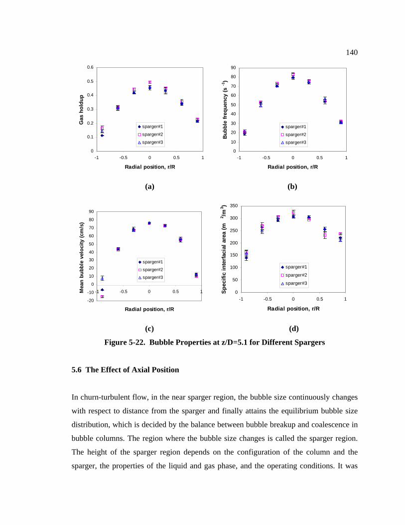
140

0

0.1

0.2

0.3

0.4

0.5

0.6

-1 -0.5 0 0.5 1


Gas

hol

dup

sparger#1

sparger#2

sparger#3

0

10

20

30

40

50

60

70

80

90

-1 -0.5 0 0.5 1


Bub

ble

frequ

ency

(s-1

)

sparger#1

sparger#2

sparger#3

(a) (b)

-20

-10

0

10

20

30

40

50

60

70

80

90

-1 -0.5 0 0.5 1


Mea

n bu

bble

vel

ocity

(cm

/s)

sparger#1

sparger#2

sparger#3

0

50

100

150

200

250

300

350

-1 -0.5 0 0.5 1


Spec

ific

inte

rfaci

al a

rea

(m2 /m

3 )

sparger#1

sparger#2

sparger#3

(c) (d)

Figure 5-22. Bubble Properties at z/D=5.1 for Different Spargers

5.6 The Effect of Axial Position

In churn-turbulent flow, in the near sparger region, the bubble size continuously changes

with respect to distance from the sparger and finally attains the equilibrium bubble size

distribution, which is decided by the balance between bubble breakup and coalescence in

bubble columns. The region where the bubble size changes is called the sparger region.

The height of the sparger region depends on the configuration of the column and the

sparger, the properties of the liquid and gas phase, and the operating conditions. It was

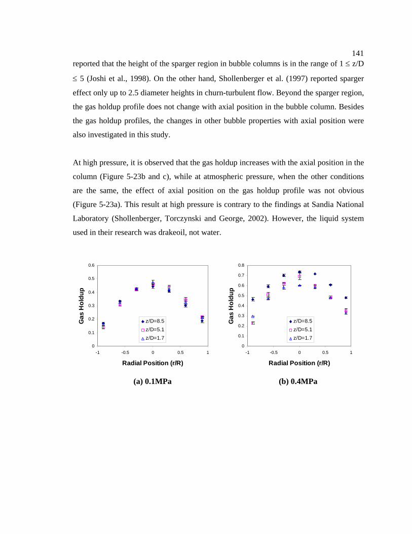
141reported that the height of the sparger region in bubble columns is in the range of 1 ≤ z/D

≤ 5 (Joshi et al., 1998). On the other hand, Shollenberger et al. (1997) reported sparger

effect only up to 2.5 diameter heights in churn-turbulent flow. Beyond the sparger region,

the gas holdup profile does not change with axial position in the bubble column. Besides

the gas holdup profiles, the changes in other bubble properties with axial position were

also investigated in this study.

At high pressure, it is observed that the gas holdup increases with the axial position in the

column (Figure 5-23b and c), while at atmospheric pressure, when the other conditions

are the same, the effect of axial position on the gas holdup profile was not obvious

(Figure 5-23a). This result at high pressure is contrary to the findings at Sandia National

Laboratory (Shollenberger, Torczynski and George, 2002). However, the liquid system

used in their research was drakeoil, not water.

0

0.1

0.2

0.3

0.4

0.5

0.6

-1 -0.5 0 0.5 1


Gas

Hol

dup

z/D=8.5z/D=5.1z/D=1.7

0

0.1

0.2

0.3

0.4

0.5

0.6

0.7

0.8

-1 -0.5 0 0.5 1


Gas

Hol

dup

z/D=8.5z/D=5.1z/D=1.7

(a) 0.1MPa (b) 0.4MPa

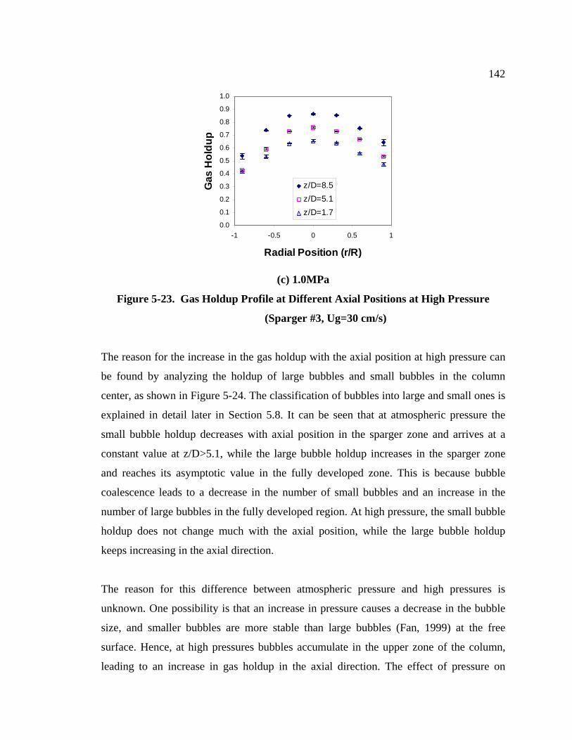
142

0.0

0.1

0.2

0.3

0.4

0.5

0.6

0.7

0.8

0.9

1.0

-1 -0.5 0 0.5 1


Gas

Hol

dup

z/D=8.5z/D=5.1z/D=1.7

(c) 1.0MPa

Figure 5-23. Gas Holdup Profile at Different Axial Positions at High Pressure

(Sparger #3, Ug=30 cm/s)

The reason for the increase in the gas holdup with the axial position at high pressure can

be found by analyzing the holdup of large bubbles and small bubbles in the column

center, as shown in Figure 5-24. The classification of bubbles into large and small ones is

explained in detail later in Section 5.8. It can be seen that at atmospheric pressure the

small bubble holdup decreases with axial position in the sparger zone and arrives at a

constant value at z/D>5.1, while the large bubble holdup increases in the sparger zone

and reaches its asymptotic value in the fully developed zone. This is because bubble

coalescence leads to a decrease in the number of small bubbles and an increase in the

number of large bubbles in the fully developed region. At high pressure, the small bubble

holdup does not change much with the axial position, while the large bubble holdup

keeps increasing in the axial direction.

The reason for this difference between atmospheric pressure and high pressures is

unknown. One possibility is that an increase in pressure causes a decrease in the bubble

size, and smaller bubbles are more stable than large bubbles (Fan, 1999) at the free

surface. Hence, at high pressures bubbles accumulate in the upper zone of the column,

leading to an increase in gas holdup in the axial direction. The effect of pressure on

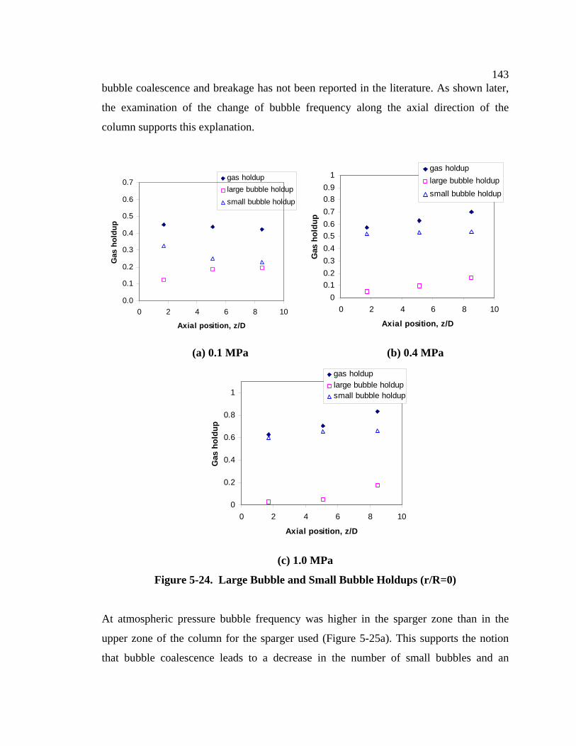
143bubble coalescence and breakage has not been reported in the literature. As shown later,

the examination of the change of bubble frequency along the axial direction of the

column supports this explanation.

0.0

0.1

0.2

0.3

0.4

0.5

0.6

0.7

0 2 4 6 8 10

Axial position, z/D

Gas

hol

dup

gas holduplarge bubble holdupsmall bubble holdup

00.10.20.30.40.50.60.70.80.9

1

0 2 4 6 8 10

Axial position, z/DG

as h

oldu

p


(a) 0.1 MPa (b) 0.4 MPa

0

0.2

0.4

0.6

0.8

1

0 2 4 6 8 1

Axial position, z/D

Gas

hol

dup

0


(c) 1.0 MPa

Figure 5-24. Large Bubble and Small Bubble Holdups (r/R=0)

At atmospheric pressure bubble frequency was higher in the sparger zone than in the

upper zone of the column for the sparger used (Figure 5-25a). This supports the notion

that bubble coalescence leads to a decrease in the number of small bubbles and an

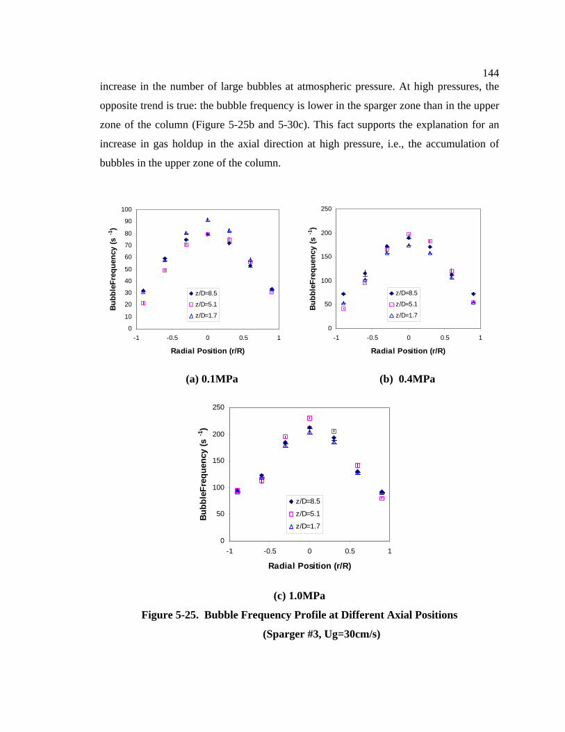
144increase in the number of large bubbles at atmospheric pressure. At high pressures, the

opposite trend is true: the bubble frequency is lower in the sparger zone than in the upper

zone of the column (Figure 5-25b and 5-30c). This fact supports the explanation for an

increase in gas holdup in the axial direction at high pressure, i.e., the accumulation of

bubbles in the upper zone of the column.

0

10

20

30

40

50

60

70

80

90

100

-1 -0.5 0 0.5 1


Bubb

leFr

eque

ncy

(s-1

)

z/D=8.5

z/D=5.1

z/D=1.7

0

50

100

150

200

250

-1 -0.5 0 0.5 1


Bub

bleF

requ

ency

(s-1

)

z/D=8.5

z/D=5.1

z/D=1.7

(a) 0.1MPa (b) 0.4MPa

0

50

100

150

200

250

-1 -0.5 0 0.5 1


Bubb

leFr

eque

ncy

(s-1

)

z/D=8.5

z/D=5.1

z/D=1.7

(c) 1.0MPa

Figure 5-25. Bubble Frequency Profile at Different Axial Positions

(Sparger #3, Ug=30cm/s)

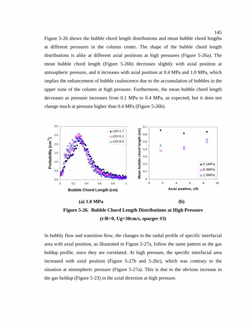
145Figure 5-26 shows the bubble chord length distributions and mean bubble chord lengths

at different pressures in the column center. The shape of the bubble chord length

distributions is alike at different axial positions at high pressures (Figure 5-26a). The

mean bubble chord length (Figure 5-26b) decreases slightly with axial position at

atmospheric pressure, and it increases with axial position at 0.4 MPa and 1.0 MPa, which

implies the enhancement of bubble coalescence due to the accumulation of bubbles in the

upper zone of the column at high pressure. Furthermore, the mean bubble chord length

decreases as pressure increases from 0.1 MPa to 0.4 MPa, as expected, but it does not

change much at pressure higher than 0.4 MPa (Figure 5-26b).

0.0

0.5

1.0

1.5

2.0

2.5

3.0

0 0.2 0.4 0.6 0.8 1


Prob

abili

ty (c

m-1

)

z/D=1.7z/D=5.1z/D=8.5

0

0.1

0.2

0.3

0.4

0.5

0.6

0.7

0 2 4 6 8 1

Axial position, z/D

Mea

n bu

bble

cho

rd le

ngth

(cm

)

0

0.1MPa0.4MPa1.0MPa

(a) 1.0 MPa (b)

Figure 5-26. Bubble Chord Length Distributions at High Pressure

(r/R=0, Ug=30cm/s, sparger #3)

In bubbly flow and transition flow, the changes in the radial profile of specific interfacial

area with axial position, as illustrated in Figure 5-27a, follow the same pattern as the gas

holdup profile, since they are correlated. At high pressure, the specific interfacial area

increased with axial position (Figure 5-27b and 5-26c), which was contrary to the

situation at atmospheric pressure (Figure 5-27a). This is due to the obvious increase in

the gas holdup (Figure 5-23) in the axial direction at high pressure.

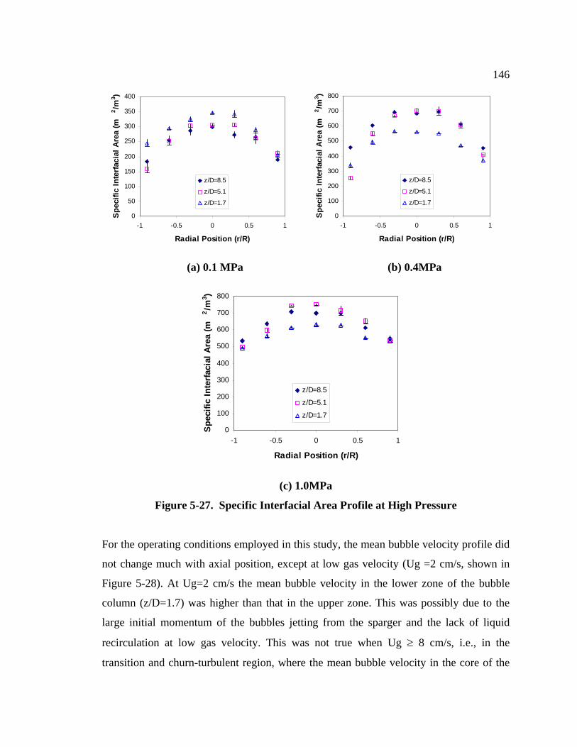
146

0

50

100

150

200

250

300

350

400

-1 -0.5 0 0.5 1


Spe

cific

Inte

rfaci

al A

rea

(m2 /m

3 )

z/D=8.5

z/D=5.1

z/D=1.7

0

100

200

300

400

500

600

700

800

-1 -0.5 0 0.5 1


Spec

ific

Inte

rfaci

al A

rea

(m2 /m

3 )

z/D=8.5

z/D=5.1

z/D=1.7

(a) 0.1 MPa (b) 0.4MPa

0

100

200

300

400

500

600

700

800

-1 -0.5 0 0.5 1


Spe

cific

Inte

rfac

ial A

rea

(m2 /m

3 )

z/D=8.5

z/D=5.1

z/D=1.7

(c) 1.0MPa

Figure 5-27. Specific Interfacial Area Profile at High Pressure

For the operating conditions employed in this study, the mean bubble velocity profile did

not change much with axial position, except at low gas velocity (Ug =2 cm/s, shown in

Figure 5-28). At Ug=2 cm/s the mean bubble velocity in the lower zone of the bubble

column (z/D=1.7) was higher than that in the upper zone. This was possibly due to the

large initial momentum of the bubbles jetting from the sparger and the lack of liquid

recirculation at low gas velocity. This was not true when Ug ≥ 8 cm/s, i.e., in the

transition and churn-turbulent region, where the mean bubble velocity in the core of the

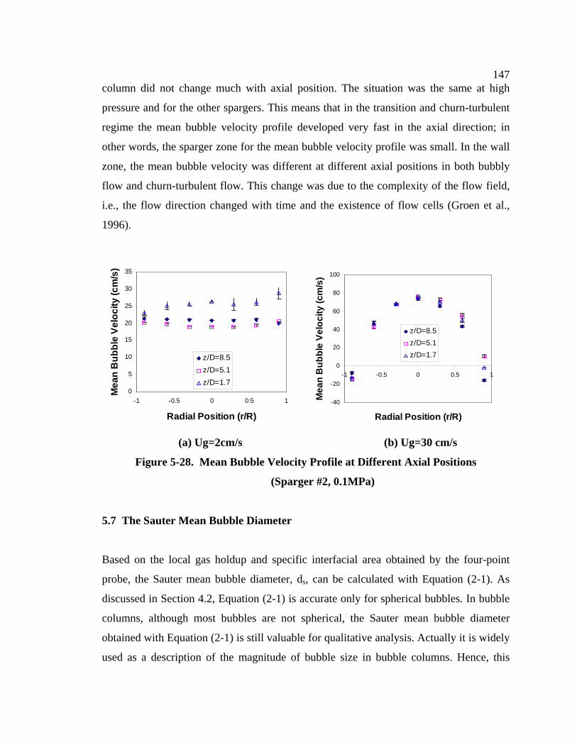
147column did not change much with axial position. The situation was the same at high

pressure and for the other spargers. This means that in the transition and churn-turbulent

regime the mean bubble velocity profile developed very fast in the axial direction; in

other words, the sparger zone for the mean bubble velocity profile was small. In the wall

zone, the mean bubble velocity was different at different axial positions in both bubbly

flow and churn-turbulent flow. This change was due to the complexity of the flow field,

i.e., the flow direction changed with time and the existence of flow cells (Groen et al.,

1996).

0

5

10

15

20

25

30

35

-1 -0.5 0 0.5 1


Mea

n B

ubbl

e Ve

loci

ty (c

m/s

)

z/D=8.5z/D=5.1z/D=1.7

-40

-20

0

20

40

60

80

100

-1 -0.5 0 0.5 1


Mea

n B

ubbl

e Ve

loci

ty (c

m/s

)z/D=8.5z/D=5.1z/D=1.7

(a) Ug=2cm/s (b) Ug=30 cm/s

Figure 5-28. Mean Bubble Velocity Profile at Different Axial Positions

(Sparger #2, 0.1MPa)

5.7 The Sauter Mean Bubble Diameter

Based on the local gas holdup and specific interfacial area obtained by the four-point

probe, the Sauter mean bubble diameter, ds, can be calculated with Equation (2-1). As

discussed in Section 4.2, Equation (2-1) is accurate only for spherical bubbles. In bubble

columns, although most bubbles are not spherical, the Sauter mean bubble diameter

obtained with Equation (2-1) is still valuable for qualitative analysis. Actually it is widely

used as a description of the magnitude of bubble size in bubble columns. Hence, this

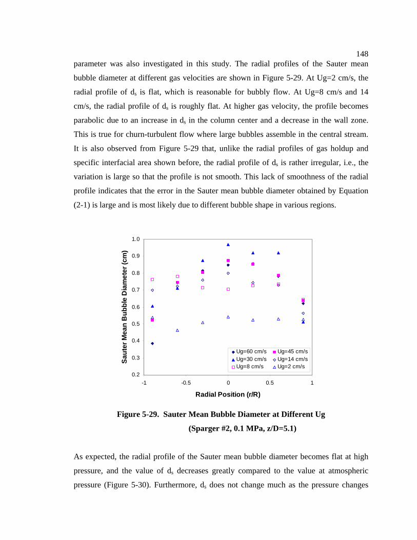
148parameter was also investigated in this study. The radial profiles of the Sauter mean

bubble diameter at different gas velocities are shown in Figure 5-29. At Ug=2 cm/s, the

radial profile of ds is flat, which is reasonable for bubbly flow. At Ug=8 cm/s and 14

cm/s, the radial profile of ds is roughly flat. At higher gas velocity, the profile becomes

parabolic due to an increase in ds in the column center and a decrease in the wall zone.

This is true for churn-turbulent flow where large bubbles assemble in the central stream.

It is also observed from Figure 5-29 that, unlike the radial profiles of gas holdup and

specific interfacial area shown before, the radial profile of ds is rather irregular, i.e., the

variation is large so that the profile is not smooth. This lack of smoothness of the radial

profile indicates that the error in the Sauter mean bubble diameter obtained by Equation

(2-1) is large and is most likely due to different bubble shape in various regions.

0.2

0.3

0.4

0.5

0.6

0.7

0.8

0.9

1.0

-1 -0.5 0 0.5 1


Saut

er M

ean

Bub

ble

Dia

met

er (c

m)

Ug=60 cm/s Ug=45 cm/sUg=30 cm/s Ug=14 cm/sUg=8 cm/s Ug=2 cm/s

Figure 5-29. Sauter Mean Bubble Diameter at Different Ug

(Sparger #2, 0.1 MPa, z/D=5.1)

As expected, the radial profile of the Sauter mean bubble diameter becomes flat at high

pressure, and the value of ds decreases greatly compared to the value at atmospheric

pressure (Figure 5-30). Furthermore, ds does not change much as the pressure changes

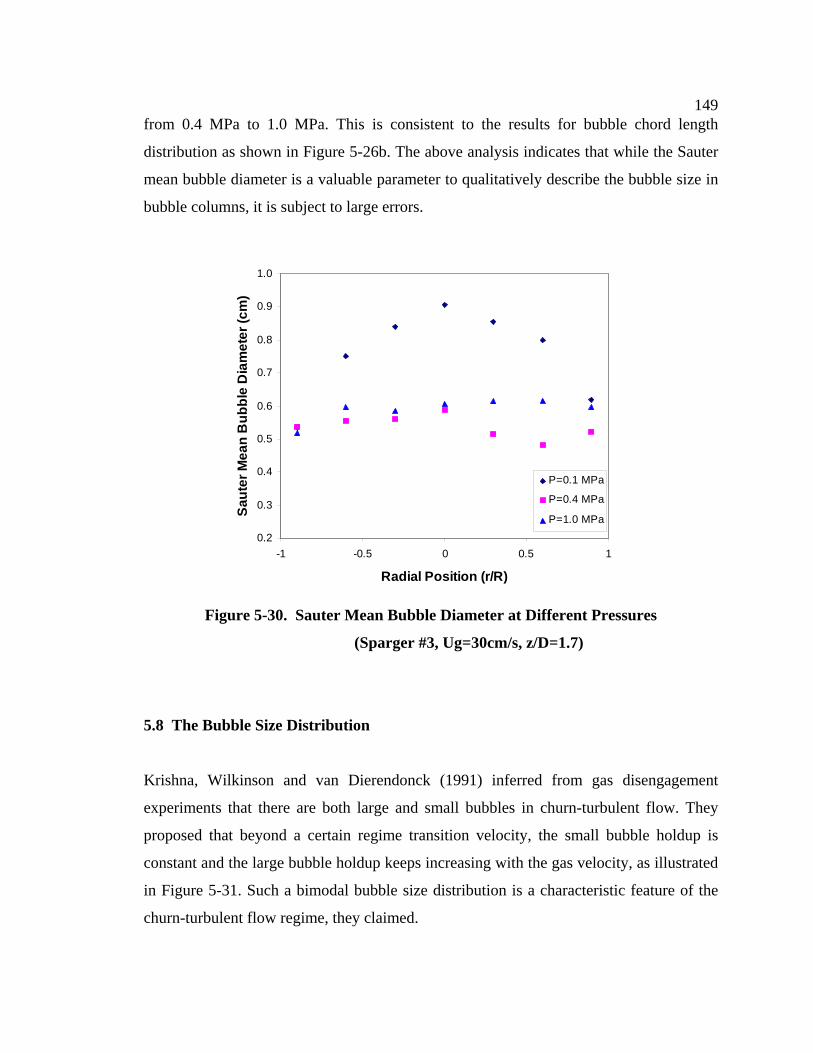
149from 0.4 MPa to 1.0 MPa. This is consistent to the results for bubble chord length

distribution as shown in Figure 5-26b. The above analysis indicates that while the Sauter

mean bubble diameter is a valuable parameter to qualitatively describe the bubble size in

bubble columns, it is subject to large errors.

0.2

0.3

0.4

0.5

0.6

0.7

0.8

0.9

1.0

-1 -0.5 0 0.5 1


Saut

er M

ean

Bub

ble

Dia

met

er (c

m)

P=0.1 MPa

P=0.4 MPa

P=1.0 MPa

Figure 5-30. Sauter Mean Bubble Diameter at Different Pressures

(Sparger #3, Ug=30cm/s, z/D=1.7)

5.8 The Bubble Size Distribution

Krishna, Wilkinson and van Dierendonck (1991) inferred from gas disengagement

experiments that there are both large and small bubbles in churn-turbulent flow. They

proposed that beyond a certain regime transition velocity, the small bubble holdup is

constant and the large bubble holdup keeps increasing with the gas velocity, as illustrated

in Figure 5-31. Such a bimodal bubble size distribution is a characteristic feature of the

churn-turbulent flow regime, they claimed.

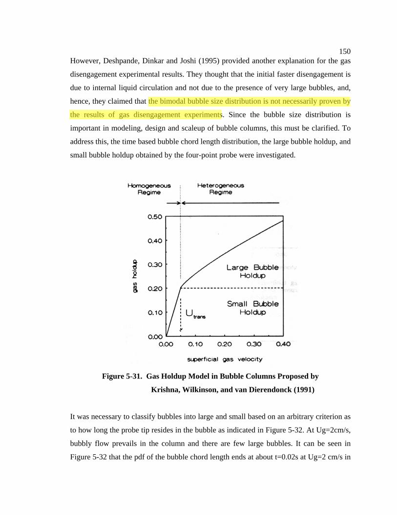
150However, Deshpande, Dinkar and Joshi (1995) provided another explanation for the gas

disengagement experimental results. They thought that the initial faster disengagement is

due to internal liquid circulation and not due to the presence of very large bubbles, and,

hence, they claimed that the bimodal bubble size distribution is not necessarily proven by

the results of gas disengagement experiments. Since the bubble size distribution is

important in modeling, design and scaleup of bubble columns, this must be clarified. To

address this, the time based bubble chord length distribution, the large bubble holdup, and

small bubble holdup obtained by the four-point probe were investigated.

Figure 5-31. Gas Holdup Model in Bubble Columns Proposed by

Krishna, Wilkinson, and van Dierendonck (1991)

It was necessary to classify bubbles into large and small based on an arbitrary criterion as

to how long the probe tip resides in the bubble as indicated in Figure 5-32. At Ug=2cm/s,

bubbly flow prevails in the column and there are few large bubbles. It can be seen in

Figure 5-32 that the pdf of the bubble chord length ends at about t=0.02s at Ug=2 cm/s in

mea2

Highlight

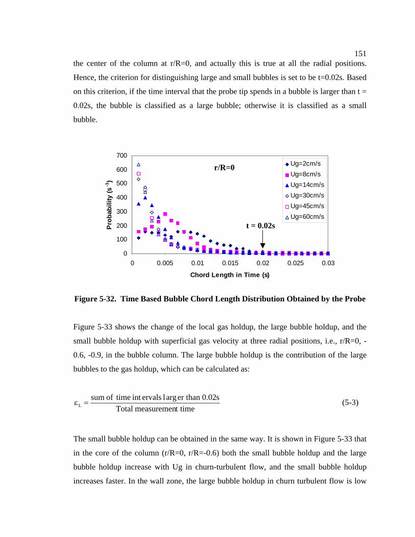
151the center of the column at r/R=0, and actually this is true at all the radial positions.

Hence, the criterion for distinguishing large and small bubbles is set to be t=0.02s. Based

on this criterion, if the time interval that the probe tip spends in a bubble is larger than t =

0.02s, the bubble is classified as a large bubble; otherwise it is classified as a small

bubble.

0

100

200

300

400

500

600

700

0 0.005 0.01 0.015

Chord Length in

Pro

babi

lity

(s-1

)

Ug=2cm/sUg=8cm/sUg=14cm/sUg=30cm/sUg=45cm/sUg=60cm/s

r/R=0

Figure 5-32. Time Based Bubble Chord Length

Figure 5-33 shows the change of the local gas hold

small bubble holdup with superficial gas velocity a

0.6, -0.9, in the bubble column. The large bubble h

bubbles to the gas holdup, which can be calculated a

timetmeasuremenTotals02.0thanerarglervalsinttimeofsum

L =ε

The small bubble holdup can be obtained in the sam

in the core of the column (r/R=0, r/R=-0.6) both th

bubble holdup increase with Ug in churn-turbulen

increases faster. In the wall zone, the large bubble

t = 0.02s

0.02 0.025 0.03

Time (s)

Distribution Obtained by the Probe

up, the large bubble holdup, and the

t three radial positions, i.e., r/R=0, -

oldup is the contribution of the large

s:

(5-3)

e way. It is shown in Figure 5-33 that

e small bubble holdup and the large

t flow, and the small bubble holdup

holdup in churn turbulent flow is low

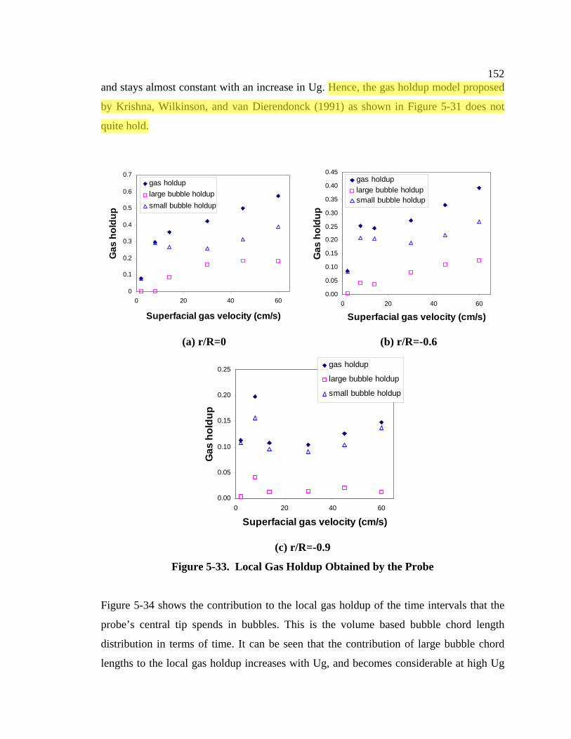
152and stays almost constant with an increase in Ug. Hence, the gas holdup model proposed

by Krishna, Wilkinson, and van Dierendonck (1991) as shown in Figure 5-31 does not

quite hold.

0

0.1

0.2

0.3

0.4

0.5

0.6

0.7

0 20 40 60

Superfacial gas velocity (cm/s)

Gas

hol

dup


0.00

0.05

0.10

0.15

0.20

0.25

0.30

0.35

0.40

0.45

0 20 40 60

Superfacial gas velocity (cm/s)G

as h

oldu

p


(a) r/R=0 (b) r/R=-0.6

0.00

0.05

0.10

0.15

0.20

0.25

0 20 40 60

Superfacial gas velocity (cm/s)

Gas

hol

dup

gas holdup

large bubble holdup

small bubble holdup

(c) r/R=-0.9

Figure 5-33. Local Gas Holdup Obtained by the Probe

Figure 5-34 shows the contribution to the local gas holdup of the time intervals that the

probe’s central tip spends in bubbles. This is the volume based bubble chord length

distribution in terms of time. It can be seen that the contribution of large bubble chord

lengths to the local gas holdup increases with Ug, and becomes considerable at high Ug

mea2

Highlight

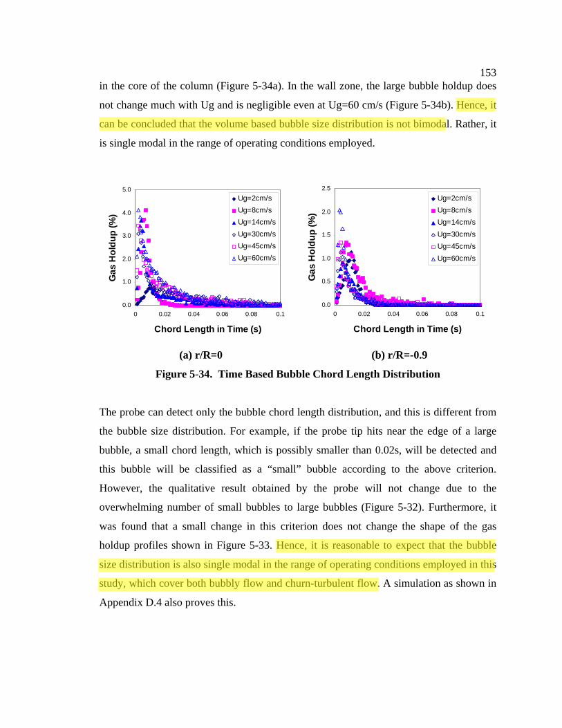
153in the core of the column (Figure 5-34a). In the wall zone, the large bubble holdup does

not change much with Ug and is negligible even at Ug=60 cm/s (Figure 5-34b). Hence, it

can be concluded that the volume based bubble size distribution is not bimodal. Rather, it

is single modal in the range of operating conditions employed.

0.0

1.0

2.0

3.0

4.0

5.0

0 0.02 0.04 0.06 0.08 0.1

Chord Length in Time (s)

Gas

Hol

dup

(%)


0.0

0.5

1.0

1.5

2.0

2.5

0 0.02 0.04 0.06 0.08 0.1


Gas

Hol

dup

(%)


(a) r/R=0 (b) r/R=-0.9

Figure 5-34. Time Based Bubble Chord Length Distribution

The probe can detect only the bubble chord length distribution, and this is different from

the bubble size distribution. For example, if the probe tip hits near the edge of a large

bubble, a small chord length, which is possibly smaller than 0.02s, will be detected and

this bubble will be classified as a “small” bubble according to the above criterion.

However, the qualitative result obtained by the probe will not change due to the

overwhelming number of small bubbles to large bubbles (Figure 5-32). Furthermore, it

was found that a small change in this criterion does not change the shape of the gas

holdup profiles shown in Figure 5-33. Hence, it is reasonable to expect that the bubble

size distribution is also single modal in the range of operating conditions employed in this

study, which cover both bubbly flow and churn-turbulent flow. A simulation as shown in

Appendix D.4 also proves this.

mea2

Highlight

mea2

Highlight

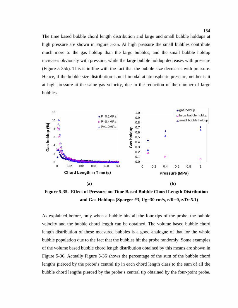
154The time based bubble chord length distribution and large and small bubble holdups at

high pressure are shown in Figure 5-35. At high pressure the small bubbles contribute

much more to the gas holdup than the large bubbles, and the small bubble holdup

increases obviously with pressure, while the large bubble holdup decreases with pressure

(Figure 5-35b). This is in line with the fact that the bubble size decreases with pressure.

Hence, if the bubble size distribution is not bimodal at atmospheric pressure, neither is it

at high pressure at the same gas velocity, due to the reduction of the number of large

bubbles.

0

2

4

6

8

10

12

0 0.02 0.04 0.06 0.08 0.1


Gas

hol

dup

(%)

P=0.1MPaP=0.4MPaP=1.0MPa

0.00.10.20.30.40.50.60.70.80.91.0

0 0.2 0.4 0.6 0.8 1

Pressure (MPa)

Gas

hol

dup


(a) (b)

Figure 5-35. Effect of Pressure on Time Based Bubble Chord Length Distribution

and Gas Holdups (Sparger #3, Ug=30 cm/s, r/R=0, z/D=5.1)

As explained before, only when a bubble hits all the four tips of the probe, the bubble

velocity and the bubble chord length can be obtained. The volume based bubble chord

length distribution of these measured bubbles is a good analogue of that for the whole

bubble population due to the fact that the bubbles hit the probe randomly. Some examples

of the volume based bubble chord length distribution obtained by this means are shown in

Figure 5-36. Actually Figure 5-36 shows the percentage of the sum of the bubble chord

lengths pierced by the probe’s central tip in each chord length class to the sum of all the

bubble chord lengths pierced by the probe’s central tip obtained by the four-point probe.

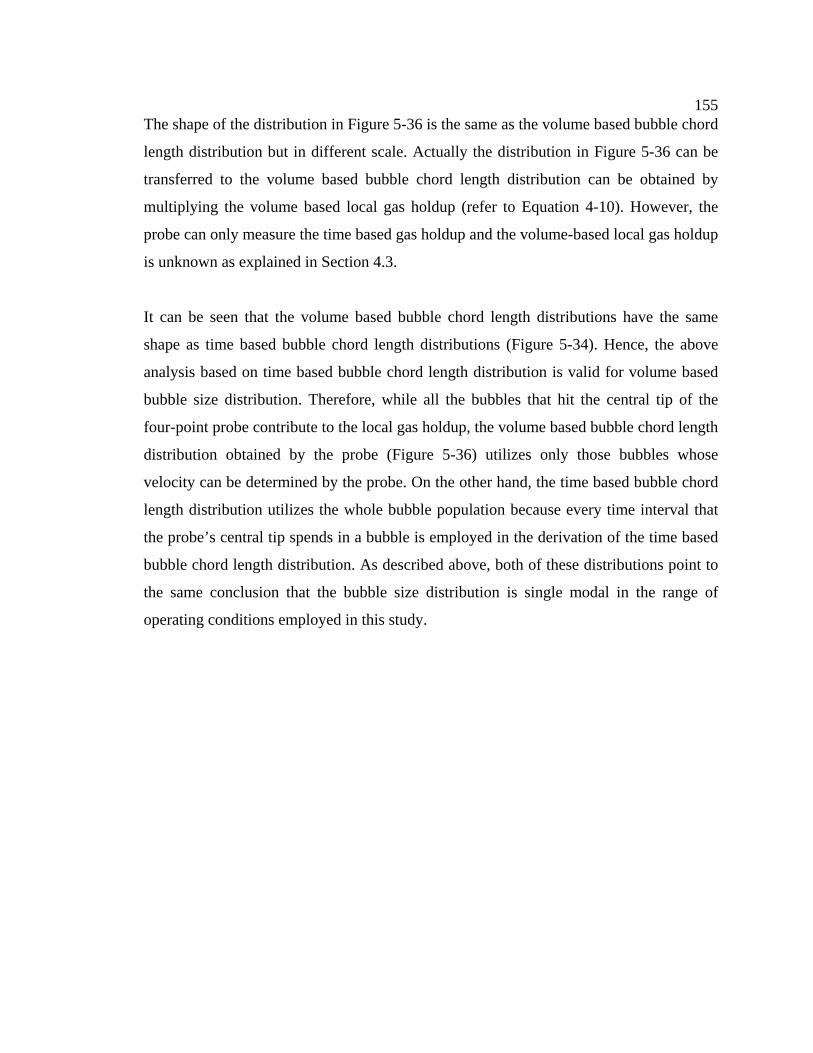
155The shape of the distribution in Figure 5-36 is the same as the volume based bubble chord

length distribution but in different scale. Actually the distribution in Figure 5-36 can be

transferred to the volume based bubble chord length distribution can be obtained by

multiplying the volume based local gas holdup (refer to Equation 4-10). However, the

probe can only measure the time based gas holdup and the volume-based local gas holdup

is unknown as explained in Section 4.3.

It can be seen that the volume based bubble chord length distributions have the same

shape as time based bubble chord length distributions (Figure 5-34). Hence, the above

analysis based on time based bubble chord length distribution is valid for volume based

bubble size distribution. Therefore, while all the bubbles that hit the central tip of the

four-point probe contribute to the local gas holdup, the volume based bubble chord length

distribution obtained by the probe (Figure 5-36) utilizes only those bubbles whose

velocity can be determined by the probe. On the other hand, the time based bubble chord

length distribution utilizes the whole bubble population because every time interval that

the probe’s central tip spends in a bubble is employed in the derivation of the time based

bubble chord length distribution. As described above, both of these distributions point to

the same conclusion that the bubble size distribution is single modal in the range of

operating conditions employed in this study.

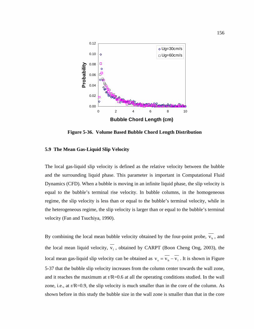
156

0.00

0.02

0.04

0.06

0.08

0.10

0.12

0 2 4 6 8 1


Prob

abili

ty

0

Ug=30cm/sUg=60cm/s

Figure 5-36. Volume Based Bubble Chord Length Distribution

5.9 The Mean Gas-Liquid Slip Velocity

The local gas-liquid slip velocity is defined as the relative velocity between the bubble

and the surrounding liquid phase. This parameter is important in Computational Fluid

Dynamics (CFD). When a bubble is moving in an infinite liquid phase, the slip velocity is

equal to the bubble’s terminal rise velocity. In bubble columns, in the homogeneous

regime, the slip velocity is less than or equal to the bubble’s terminal velocity, while in

the heterogeneous regime, the slip velocity is larger than or equal to the bubble’s terminal

velocity (Fan and Tsuchiya, 1990).

By combining the local mean bubble velocity obtained by the four-point probe, bv , and

the local mean liquid velocity, lv , obtained by CARPT (Boon Cheng Ong, 2003), the

local mean gas-liquid slip velocity can be obtained as lbs vvv −= . It is shown in Figure

5-37 that the bubble slip velocity increases from the column center towards the wall zone,

and it reaches the maximum at r/R=0.6 at all the operating conditions studied. In the wall

zone, i.e., at r/R=0.9, the slip velocity is much smaller than in the core of the column. As

shown before in this study the bubble size in the wall zone is smaller than that in the core

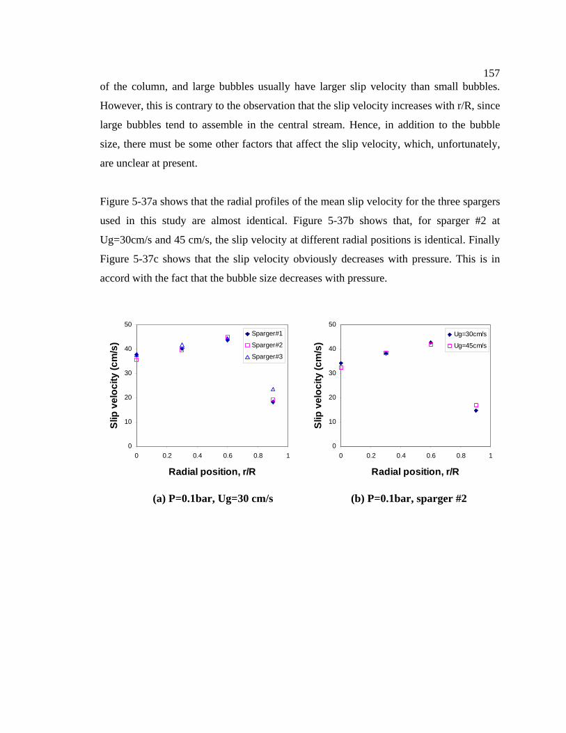
157of the column, and large bubbles usually have larger slip velocity than small bubbles.

However, this is contrary to the observation that the slip velocity increases with r/R, since

large bubbles tend to assemble in the central stream. Hence, in addition to the bubble

size, there must be some other factors that affect the slip velocity, which, unfortunately,

are unclear at present.

Figure 5-37a shows that the radial profiles of the mean slip velocity for the three spargers

used in this study are almost identical. Figure 5-37b shows that, for sparger #2 at

Ug=30cm/s and 45 cm/s, the slip velocity at different radial positions is identical. Finally

Figure 5-37c shows that the slip velocity obviously decreases with pressure. This is in

accord with the fact that the bubble size decreases with pressure.

0

10

20

30

40

50

0 0.2 0.4 0.6 0.8 1


Slip

vel

ocity

(cm

/s)

Sparger#1

Sparger#2

Sparger#3

0

10

20

30

40

50

0 0.2 0.4 0.6 0.8 1


Slip

vel

ocity

(cm

/s)

Ug=30cm/s

Ug=45cm/s

(a) P=0.1bar, Ug=30 cm/s (b) P=0.1bar, sparger #2

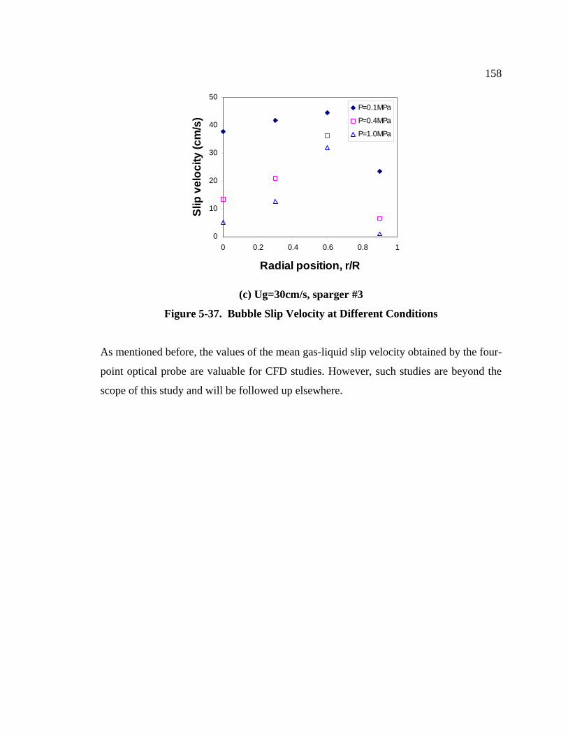
158

0

10

20

30

40

50

0 0.2 0.4 0.6 0.8 1


Slip

vel

ocity

(cm

/s)

P=0.1MPa

P=0.4MPa

P=1.0MPa

(c) Ug=30cm/s, sparger #3

Figure 5-37. Bubble Slip Velocity at Different Conditions

As mentioned before, the values of the mean gas-liquid slip velocity obtained by the four-

point optical probe are valuable for CFD studies. However, such studies are beyond the

scope of this study and will be followed up elsewhere.

159

Chapter 6 Conclusions and Future Work

The following conclusions can be derived from this study:

1. Two-point probes produce questionable results in systems having complex

hydrodynamics, such as bubble columns, especially in transition and churn-turbulent flow

regime.

2. The four-point optical probe and the new data processing algorithm is a practical tool

for investigating bubble properties in bubble columns. By validation against video

imaging, it was proved that the bubble velocity distribution, bubble chord length

distribution, local gas holdup, and specific interfacial area obtained by the new four-point

optical probe algorithm are reliable. Difficulties exist in the measurements of bubbles of

very low velocity approximating to zero.

3. The four-point optical probe performed well both in bubbly flow and in highly churn-

turbulent flow at superficial gas velocity up to 60 cm/s and pressure up to 1.0 MPa.

Bubble properties at these conditions in a 6.4” bubble column were measured for the first

time, which are valuable for CFD validation and for development of engineering models.

4. Some new findings about bubble properties in bubble columns are:

(1). In bubbly flow, the radial profiles of specific interfacial area, bubble frequency,

and mean bubble velocity are all flat. With an increase in superficial gas

velocity, Ug, these profiles became more parabolic. In the column center, the

bubble chord length distribution spreads wider with an increase in Ug. The mean

bubble chord length increases with Ug until it is in deep churn-turbulent flow

and then remains almost identical with Ug. In the wall region, the bubble chord

length distribution does not change much with Ug. The mean bubble chord

160length in the wall region is much smaller than that in the column center, and it

increases mildly with Ug between the bubbly flow and the transition flow

regime, then decrease slightly with Ug.

(2). At very low gas velocity, e.g. 2 cm/s, all bubbles move upwards in bubble

column. In churn-turbulent flow (Ug>8cm/s), some bubbles move downwards

even in the column center. In the wall region, the number of bubbles moving

downwards is equal to or even larger than that of bubbles moving upwards. The

percentage of bubbles moving downwards increases slowly with Ug in both the

wall region and in the core of the column. In the wall region, the bubbles moving

downwards are dragged down by the liquid, while in the core of the column the

flow direction is generally upwards most of the time, and the bubbles moving

downwards most likely come from the wakes of large bubbles and large 3D flow

structures.

(3). In bubbly flow, the bubble velocity distribution and bubble chord length

distribution are alike at different radial positions, including the wall region. In

churn-turbulent flow, in the core of the column the bubble velocity and chord

length distributions are alike at different radial position, but in the wall region

they are very different from the core of the column.

(4). With an increase in pressure, the global liquid recirculation is enhanced, and the

radial profiles of specific interfacial area, bubble frequency, and mean bubble

velocity become more parabolic. The gas holdup increases with the axial position,

possibly due to the accumulation of bubbles at the upper zone of the column at

high pressure. The pressure effect is strong at 0.1 MPa, but it becomes weaker at

pressures higher than 0.4 MPa.

(5). Two of the three spargers used in this study, i.e. sparger#1 and sparger#3,

generated similar bubble properties at the operating conditions employed,

161although their configurations are totally different. Sparger#2 generates somewhat

different bubble properties than the other two spargers, though not to a significant

extent.

(6). In this study, the sparger effect disappears with an increase in the axial position in

bubble column at z/D>5.1. However, at atmospheric pressure, the range of the

sparger zone for the specific interfacial area is beyond z/D=5. Hence, the

definition of the sparger zone based on gas holdup profiles may not apply to other

bubble properties under some conditions. In other words, the range of the sparger

zone for different bubble properties may be different.

(7). The Sauter mean bubble diameter cannot be calculated without assumptions that

are not met and it is subject to large errors. Qualitatively it can be used for

comparison of “mean” bubble size at different conditions.

(8). The bubble size distributions observed are single modal. Hence, the suggested

bimodal bubble size distribution postulated for churn-turbulent flow was not

detected.

(9). In this study, the mean gas-liquid slip velocity is almost identical for different

spargers and at different superficial gas velocities in churn-turbulent flow, it

decreases with pressure, due to a decrease in the bubble size.

Suggested future work to fully utilize the power of the four-point optical probe technique:

1. Use bubble properties data obtained by the four-point optical probe for validation and

refinement of CFD codes.

2. Apply the four-point optical probe to a wider range of operating conditions, such as the

superficial gas velocity, pressure, column diameter, and spargers, etc., to expand the

162bubble properties data base and get a better understanding of the hydrodynamics in

bubble columns. Besides, apply the four-point optical probe to multiphase reactors other

than bubble column, e.g., stirred tank reactors.

3. Validate and apply the four-point probe in organic systems of industrial interest. In

addition, apply the four-point probe at high temperature and pressure higher than 1.0

MPa. Exploit the potential of the probe technique to detect phase transition at

supercritical conditions (see Appendix E).

4. Apply the probe in slurry bubble columns to test the durability of the probe against the

collision of the particles. In the cases that the glass probe cannot stand long enough, e.g.

systems with solid particles and high gas velocity, the plastic probe described in

Appendix A should be used.

5. Commercialize the four-point probe technique to provide a tool which is simple and

easy to use for the on site measurements of bubble properties, e.g. monitor the quality of

the flow in multiphase reactors.

163

Appendix A The Plastic Fiber Optical Probe

An optical fiber probe made of plastic fibers (Polymethyl Meta Acrylate) was also

developed in this research according to the methods employed by Saito and Mudde

(2001). The fabrication of the plastic fiber probe is almost the same as that of the glass

fiber probe, except that the tip of the plastic fiber is cut into a wedge of 30o (Figure

3.14a), which is the optimal angle determined by trail and error, instead of being made

conical with a flame as in the case with the glass fiber.

The plastic probe has the advantage over the glass probe that the size is small since there

isn’t any protective cladding cover on it (the outer diameter of plastic fibers used is

0.25mm, compared with 0.6mm for glass fibers). The smaller size of the probe reduces

the disturbance of the probe to the flow field and makes the probe detects smaller

bubbles. Furthermore, it is much more durable than the glass fiber probe due to the

flexibility of the plastic fiber. Therefore, the plastic probe may be more suitable for use in

slurry bubble columns where the glass probe may be broken by the particles in turbulent

motion.

It can be seen from Figure 3.14b that the output voltage of the plastic fiber probe is low

when the tip is in a bubble, and it is high when the tip is in the liquid phase, which is

contrary to that of a glass fiber probe. This is determined by the characteristic of the

photoelectric multiplier used. The processing of the responses is the same as that for the

glass optical probe.

The disadvantages of the plastic fiber probe are: (1) It cannot endure high temperature

(the permanent usage temperature of the plastic fiber used is 75oC). (2) Some organic

solution may do harm to the plastic fiber, this limits its application in organic systems.

And (3) the flexibility of the fiber makes it tremble in turbulent flow, this will cause

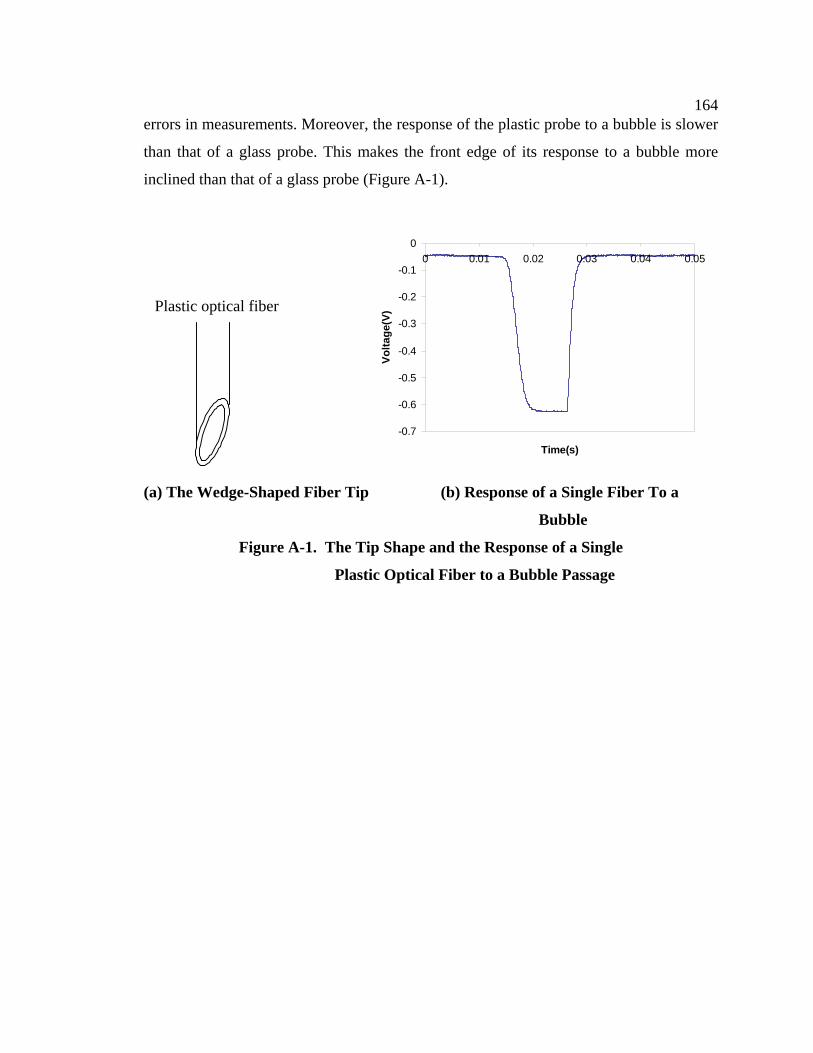
164errors in measurements. Moreover, the response of the plastic probe to a bubble is slower

than that of a glass probe. This makes the front edge of its response to a bubble more

inclined than that of a glass probe (Figure A-1).

Plastic optical fiber

-0.7

-0.6

-0.5

-0.4

-0.3

-0.2

-0.1

00 0.01 0.02 0.03 0.04 0.05

Time(s)

Volta

ge(V

)

(a) The Wedge-Shaped Fiber Tip (b) Response of a Single Fiber To a

Bubble

Figure A-1. The Tip Shape and the Response of a Single

Plastic Optical Fiber to a Bubble Passage

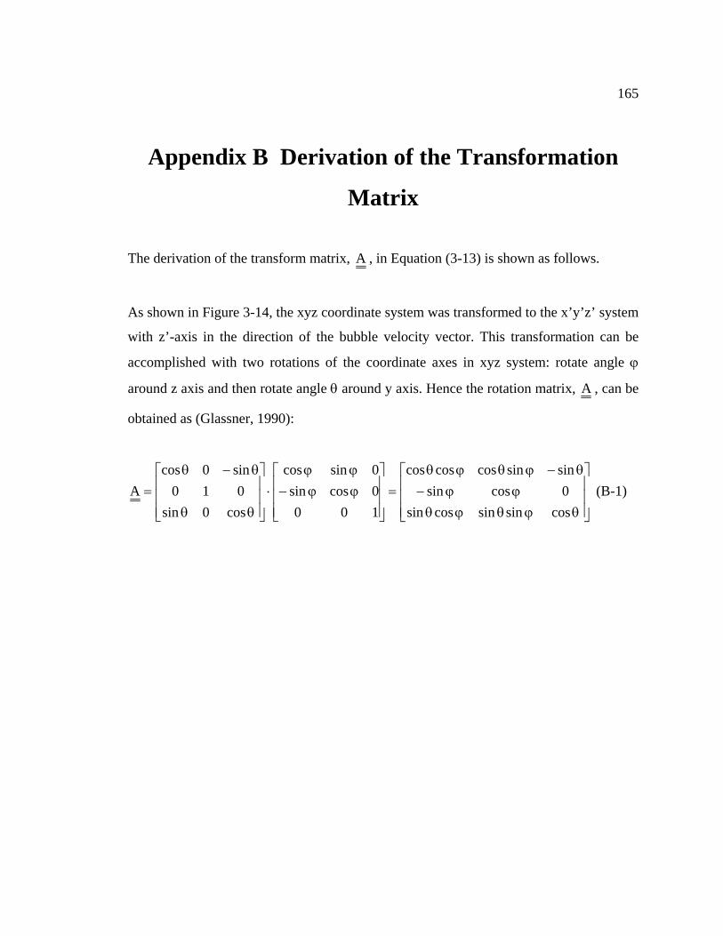
165

Appendix B Derivation of the Transformation

Matrix

The derivation of the transform matrix, A , in Equation (3-13) is shown as follows.

As shown in Figure 3-14, the xyz coordinate system was transformed to the x’y’z’ system

with z’-axis in the direction of the bubble velocity vector. This transformation can be

accomplished with two rotations of the coordinate axes in xyz system: rotate angle ϕ

around z axis and then rotate angle θ around y axis. Hence the rotation matrix, A , can be

obtained as (Glassner, 1990):

⎥⎥⎥

⎦

⎤

⎢⎢⎢

⎣

⎡

θϕθϕθϕϕ−

θ−ϕθϕθ=

⎥⎥⎥

⎦

⎤

⎢⎢⎢

⎣

⎡ϕϕ−ϕϕ

⋅⎥⎥⎥

⎦

⎤

⎢⎢⎢

⎣

⎡

θθ

θ−θ=

cossinsincossin0cossin

sinsincoscoscos

1000cossin0sincos

cos0sin010

sin0cosA (B-1)

166

Appendix C The Natural Frequency of the

Optical Probe

To check the possibility of resonance of the glass optical probe in multiphase flow, the

natural frequency of the probe was calculated.

The formula for the natural frequency is (Condon and Odishaw, 1967):

ρ=

EL21f (C-1)

where f is the natural frequency, L and ρ are the length and the density of the object

(probe), and E is the Youngs modulus of the material of which the object (probe) is made.

The physical properties of the glass optical fiber used in this study are: L≈1.5cm,

ρ=2.203 g/cm3, and E=5.8×109 Kg/m2. Hence, the natural frequency of the optical fiber is

about 54 KHz, which is much higher than the bubble frequency in multiphase systems

(usually in the range of 0~1000 Hz). Hence, the glass optical probe used in this study

does not resonate in the bubble column flows.

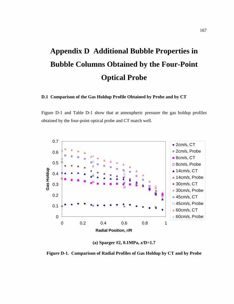
167

Appendix D Additional Bubble Properties in

Bubble Columns Obtained by the Four-Point

Optical Probe

D.1 Comparison of the Gas Holdup Profile Obtained by Probe and by CT

Figure D-1 and Table D-1 show that at atmospheric pressure the gas holdup profiles

obtained by the four-point optical probe and CT match well.

0

0.1

0.2

0.3

0.4

0.5

0.6

0.7

0 0.2 0.4 0.6 0.8 1Radial Position, r/R

Gas

Hol

dup


(a) Sparger #2, 0.1MPa, z/D=1.7

Figure D-1. Comparison of Radial Profiles of Gas Holdup by CT and by Probe

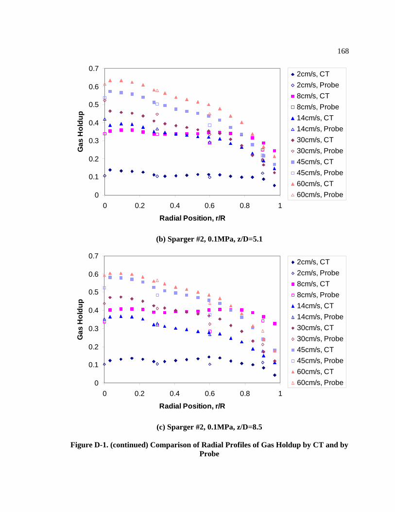
168

0

0.1

0.2

0.3

0.4

0.5

0.6

0.7

0 0.2 0.4 0.6 0.8 1


Gas

Hol

dup


(b) Sparger #2, 0.1MPa, z/D=5.1

0

0.1

0.2

0.3

0.4

0.5

0.6

0.7

0 0.2 0.4 0.6 0.8 1


Gas

Hol

dup


(c) Sparger #2, 0.1MPa, z/D=8.5

Figure D-1. (continued) Comparison of Radial Profiles of Gas Holdup by CT and by

Probe

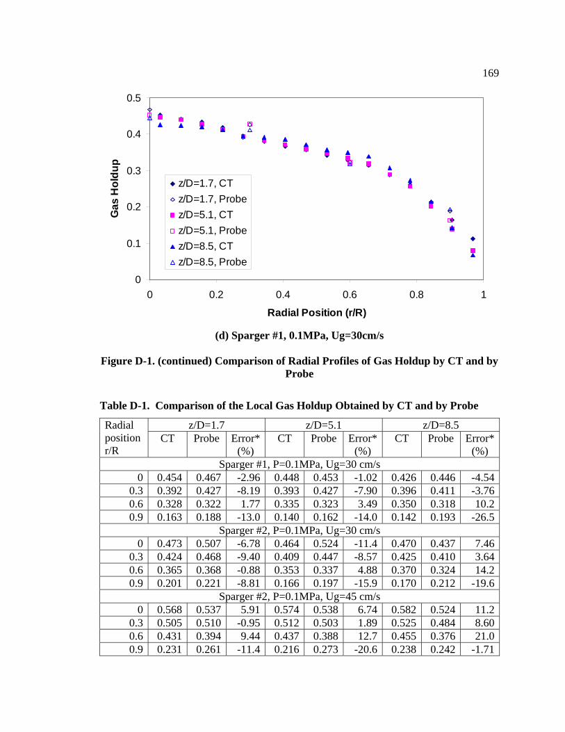
169

0

0.1

0.2

0.3

0.4

0.5

0 0.2 0.4 0.6 0.8 1


Gas

Hol

dup

z/D=1.7, CTz/D=1.7, Probez/D=5.1, CTz/D=5.1, Probez/D=8.5, CTz/D=8.5, Probe

(d) Sparger #1, 0.1MPa, Ug=30cm/s

Figure D-1. (continued) Comparison of Radial Profiles of Gas Holdup by CT and by

Probe

Table D-1. Comparison of the Local Gas Holdup Obtained by CT and by Probe

z/D=1.7 z/D=5.1 z/D=8.5 Radial position r/R

CT

Probe

Error*(%)

CT

Probe

Error* (%)

CT

Probe

Error* (%)

Sparger #1, P=0.1MPa, Ug=30 cm/s 0 0.454 0.467 -2.96 0.448 0.453 -1.02 0.426 0.446 -4.54

0.3 0.392 0.427 -8.19 0.393 0.427 -7.90 0.396 0.411 -3.760.6 0.328 0.322 1.77 0.335 0.323 3.49 0.350 0.318 10.20.9 0.163 0.188 -13.0 0.140 0.162 -14.0 0.142 0.193 -26.5

Sparger #2, P=0.1MPa, Ug=30 cm/s 0 0.473 0.507 -6.78 0.464 0.524 -11.4 0.470 0.437 7.46

0.3 0.424 0.468 -9.40 0.409 0.447 -8.57 0.425 0.410 3.640.6 0.365 0.368 -0.88 0.353 0.337 4.88 0.370 0.324 14.20.9 0.201 0.221 -8.81 0.166 0.197 -15.9 0.170 0.212 -19.6

Sparger #2, P=0.1MPa, Ug=45 cm/s 0 0.568 0.537 5.91 0.574 0.538 6.74 0.582 0.524 11.2

0.3 0.505 0.510 -0.95 0.512 0.503 1.89 0.525 0.484 8.600.6 0.431 0.394 9.44 0.437 0.388 12.7 0.455 0.376 21.00.9 0.231 0.261 -11.4 0.216 0.273 -20.6 0.238 0.242 -1.71

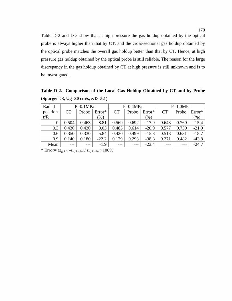
170Table D-2 and D-3 show that at high pressure the gas holdup obtained by the optical

probe is always higher than that by CT, and the cross-sectional gas holdup obtained by

the optical probe matches the overall gas holdup better than that by CT. Hence, at high

pressure gas holdup obtained by the optical probe is still reliable. The reason for the large

discrepancy in the gas holdup obtained by CT at high pressure is still unknown and is to

be investigated.

Table D-2. Comparison of the Local Gas Holdup Obtained by CT and by Probe

(Sparger #3, Ug=30 cm/s, z/D=5.1)

P=0.1MPa P=0.4MPa P=1.0MPa Radial position r/R

CT

Probe

Error*(%)

CT

Probe

Error* (%)

CT

Probe

Error* (%)

0 0.504 0.463 8.81 0.569 0.692 -17.9 0.643 0.760 -15.40.3 0.430 0.430 0.03 0.485 0.614 -20.9 0.577 0.730 -21.00.6 0.350 0.330 5.84 0.420 0.499 -15.8 0.513 0.631 -18.70.9 0.140 0.180 -22.2 0.179 0.293 -38.8 0.271 0.482 -43.8

Mean --- --- -1.9 --- --- -23.4 --- --- -24.7* Error= (εg, CT -εg, Probe)/ εg, Probe ×100%

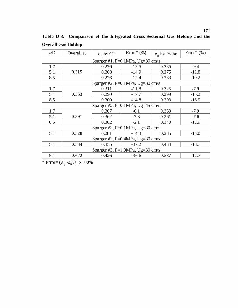
171Table D-3. Comparison of the Integrated Cross-Sectional Gas Holdup and the

Overall Gas Holdup

z/D Overall εg gε by CT Error* (%) gε by Probe Error* (%)

Sparger #1, P=0.1MPa, Ug=30 cm/s 1.7 0.276 -12.5 0.285 -9.4 5.1 0.268 -14.9 0.275 -12.8 8.5

0.315 0.276 -12.4 0.283 -10.2


0.353 0.300 -14.8 0.293 -16.9


0.391 0.382 -2.1 0.340 -12.9

Sparger #3, P=0.1MPa, Ug=30 cm/s 5.1 0.328 0.281 -14.3 0.285 -13.0



* Error= ( gε -εg)/εg ×100%

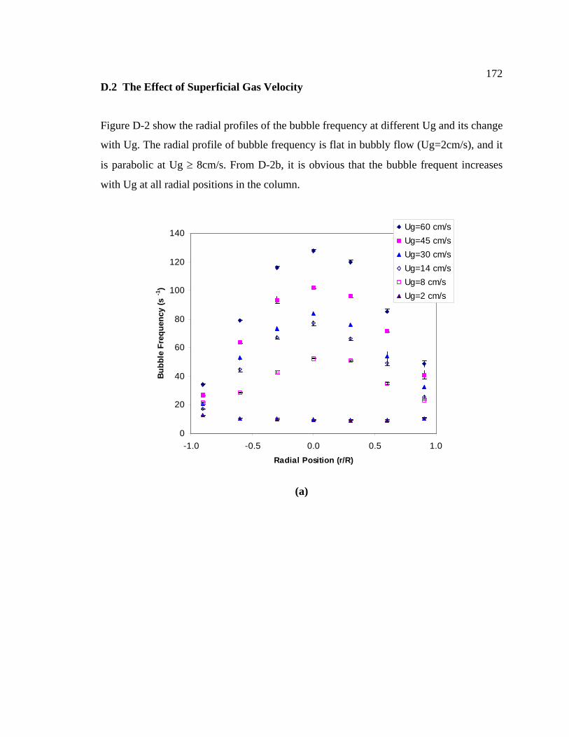
172D.2 The Effect of Superficial Gas Velocity

Figure D-2 show the radial profiles of the bubble frequency at different Ug and its change

with Ug. The radial profile of bubble frequency is flat in bubbly flow (Ug=2cm/s), and it

is parabolic at Ug ≥ 8cm/s. From D-2b, it is obvious that the bubble frequent increases

with Ug at all radial positions in the column.

0

20

40

60

80

100

120

140

-1.0 -0.5 0.0 0.5 1.0Radial Position (r/R)

Bubb

le F

requ

ency

(s-1

)


(a)

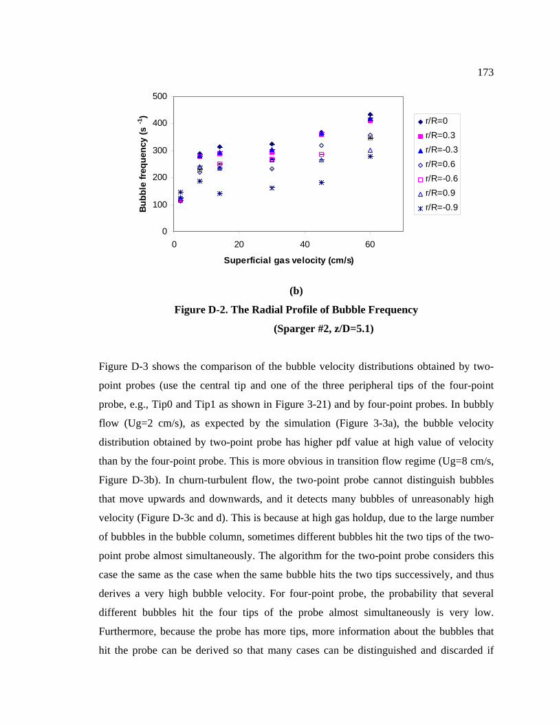
173

0

100

200

300

400

500

0 20 40 60

Superficial gas velocity (cm/s)

Bubb

le fr

eque

ncy

(s-1

) r/R=0r/R=0.3r/R=-0.3r/R=0.6r/R=-0.6r/R=0.9r/R=-0.9

(b)

Figure D-2. The Radial Profile of Bubble Frequency


Figure D-3 shows the comparison of the bubble velocity distributions obtained by two-

point probes (use the central tip and one of the three peripheral tips of the four-point

probe, e.g., Tip0 and Tip1 as shown in Figure 3-21) and by four-point probes. In bubbly

flow (Ug=2 cm/s), as expected by the simulation (Figure 3-3a), the bubble velocity

distribution obtained by two-point probe has higher pdf value at high value of velocity

than by the four-point probe. This is more obvious in transition flow regime (Ug=8 cm/s,

Figure D-3b). In churn-turbulent flow, the two-point probe cannot distinguish bubbles

that move upwards and downwards, and it detects many bubbles of unreasonably high

velocity (Figure D-3c and d). This is because at high gas holdup, due to the large number

of bubbles in the bubble column, sometimes different bubbles hit the two tips of the two-

point probe almost simultaneously. The algorithm for the two-point probe considers this

case the same as the case when the same bubble hits the two tips successively, and thus

derives a very high bubble velocity. For four-point probe, the probability that several

different bubbles hit the four tips of the probe almost simultaneously is very low.

Furthermore, because the probe has more tips, more information about the bubbles that

hit the probe can be derived so that many cases can be distinguished and discarded if

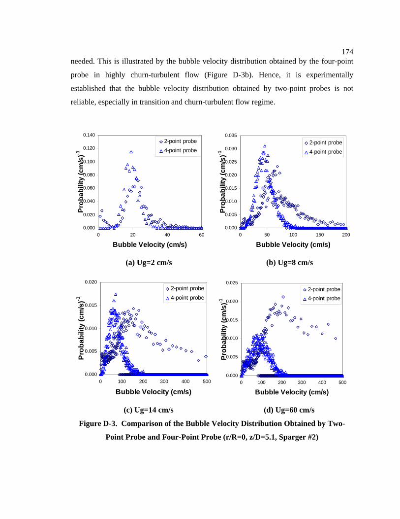
174needed. This is illustrated by the bubble velocity distribution obtained by the four-point

probe in highly churn-turbulent flow (Figure D-3b). Hence, it is experimentally

established that the bubble velocity distribution obtained by two-point probes is not

reliable, especially in transition and churn-turbulent flow regime.

0.000

0.020

0.040

0.060

0.080

0.100

0.120

0.140

0 20 40 600.000

0.005

0.010

0.015

0.020

0.025

0.030

0.035

0 50 100 150 200


Prob

abili

ty (c

m/s

)-1

2-point probe4-point probe


Prob

abili

ty (c

m/s

)-1



0.000

0.005

0.010

0.015

0.020

0 100 200 300 400 500


Prob

abili

ty (c

m/s

)-1


0.000

0.005

0.010

0.015

0.020

0.025

0 100 200 300 400 500


Prob

abili

ty (c

m/s

)-1



Figure D-3. Comparison of the Bubble Velocity Distribution Obtained by Two-

Point Probe and Four-Point Probe (r/R=0, z/D=5.1, Sparger #2)

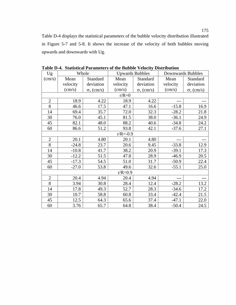
175Table D-4 displays the statistical parameters of the bubble velocity distribution illustrated

in Figure 5-7 and 5-8. It shows the increase of the velocity of both bubbles moving

upwards and downwards with Ug.

Table D-4. Statistical Parameters of the Bubble Velocity Distribution Whole Upwards Bubbles Downwards Bubbles Ug

(cm/s) Mean velocity (cm/s)

Standard deviation σ, (cm/s)

Mean velocity (cm/s)


Mean velocity (cm/s)


r/R=0 2 18.9 4.22 18.9 4.22 --- ---8 46.6 17.5 47.1 16.6 -15.8 16.914 69.4 35.7 72.0 32.3 -28.2 21.830 76.0 45.1 81.5 38.0 -36.1 24.945 82.1 48.0 88.2 40.6 -34.8 24.260 86.6 51.2 93.8 42.1 -37.6 27.1

r/R=-0.9 2 20.1 4.80 20.1 4.80 --- ---8 -24.8 23.7 20.6 9.45 -33.8 12.914 -10.8 41.7 38.2 20.9 -39.1 17.330 -12.2 51.5 47.8 28.9 -46.9 20.545 -17.3 54.5 51.0 31.7 -50.9 22.460 -27.0 53.8 49.6 32.6 -55.1 25.0

r/R=0.9 2 20.4 4.94 20.4 4.94 --- ---8 3.94 30.8 28.4 12.4 -28.2 13.214 17.8 49.3 52.7 28.3 -34.6 17.230 10.7 58.8 60.8 33.4 -42.4 21.545 12.5 64.3 65.6 37.4 -47.1 22.060 3.76 65.7 64.8 38.4 -50.4 24.5

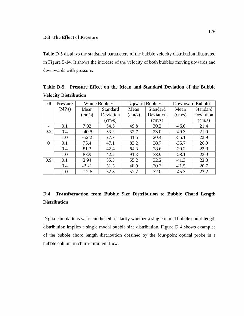
176D.3 The Effect of Pressure

Table D-5 displays the statistical parameters of the bubble velocity distribution illustrated

in Figure 5-14. It shows the increase of the velocity of both bubbles moving upwards and

downwards with pressure.

Table D-5. Pressure Effect on the Mean and Standard Deviation of the Bubble

Velocity Distribution

Whole Bubbles Upward Bubbles Downward Bubbles r/R Pressure (MPa) Mean

(cm/s) Standard Deviation

(cm/s)

Mean (cm/s)

Standard Deviation

(cm/s)

Mean (cm/s)

Standard Deviation

(cm/s) 0.1 7.92 54.5 49.8 30.2 -46.0 21.4 0.4 -40.5 33.2 32.7 23.0 -49.3 21.0

-0.9

1.0 -52.2 27.7 31.5 20.4 -55.1 22.9 0.1 76.4 47.1 83.2 38.7 -35.7 26.9 0.4 81.3 42.4 84.3 38.6 -30.3 23.8

0

1.0 88.9 42.2 91.3 38.9 -28.1 23.9 0.1 2.94 55.3 55.2 32.2 -41.3 22.3 0.4 -2.21 51.5 48.9 30.3 -41.5 20.7

0.9

1.0 -12.6 52.8 52.2 32.0 -45.3 22.2

D.4 Transformation from Bubble Size Distribution to Bubble Chord Length

Distribution

Digital simulations were conducted to clarify whether a single modal bubble chord length

distribution implies a single modal bubble size distribution. Figure D-4 shows examples

of the bubble chord length distribution obtained by the four-point optical probe in a

bubble column in churn-turbulent flow.

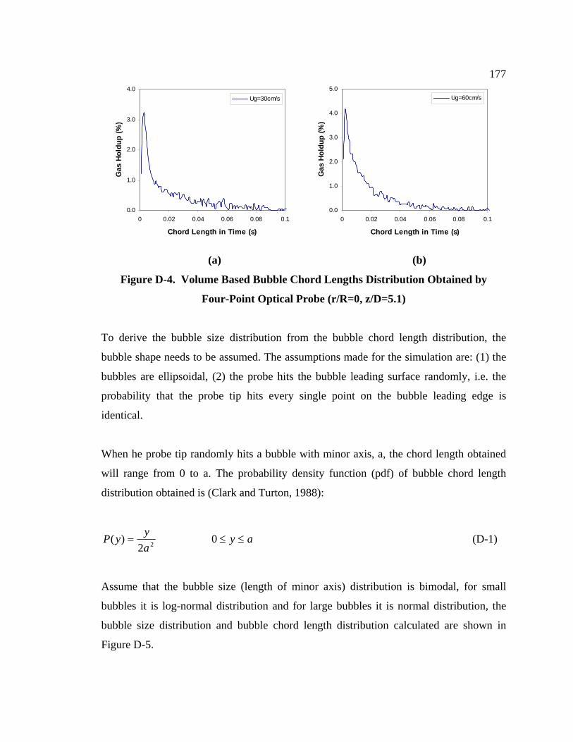
177

0.0

1.0

2.0

3.0

4.0

0 0.02 0.04 0.06 0.08 0.1


Gas

Hol

dup

(%)

Ug=30cm/s

0.0

1.0

2.0

3.0

4.0

5.0

0 0.02 0.04 0.06 0.08 0.1


Gas

Hol

dup

(%)

Ug=60cm/s

(a) (b)

Figure D-4. Volume Based Bubble Chord Lengths Distribution Obtained by

Four-Point Optical Probe (r/R=0, z/D=5.1)

To derive the bubble size distribution from the bubble chord length distribution, the

bubble shape needs to be assumed. The assumptions made for the simulation are: (1) the

bubbles are ellipsoidal, (2) the probe hits the bubble leading surface randomly, i.e. the

probability that the probe tip hits every single point on the bubble leading edge is

identical.

When he probe tip randomly hits a bubble with minor axis, a, the chord length obtained

will range from 0 to a. The probability density function (pdf) of bubble chord length

distribution obtained is (Clark and Turton, 1988):

ayayyP ≤≤= 0

2)( 2 (D-1)

Assume that the bubble size (length of minor axis) distribution is bimodal, for small

bubbles it is log-normal distribution and for large bubbles it is normal distribution, the

bubble size distribution and bubble chord length distribution calculated are shown in

Figure D-5.

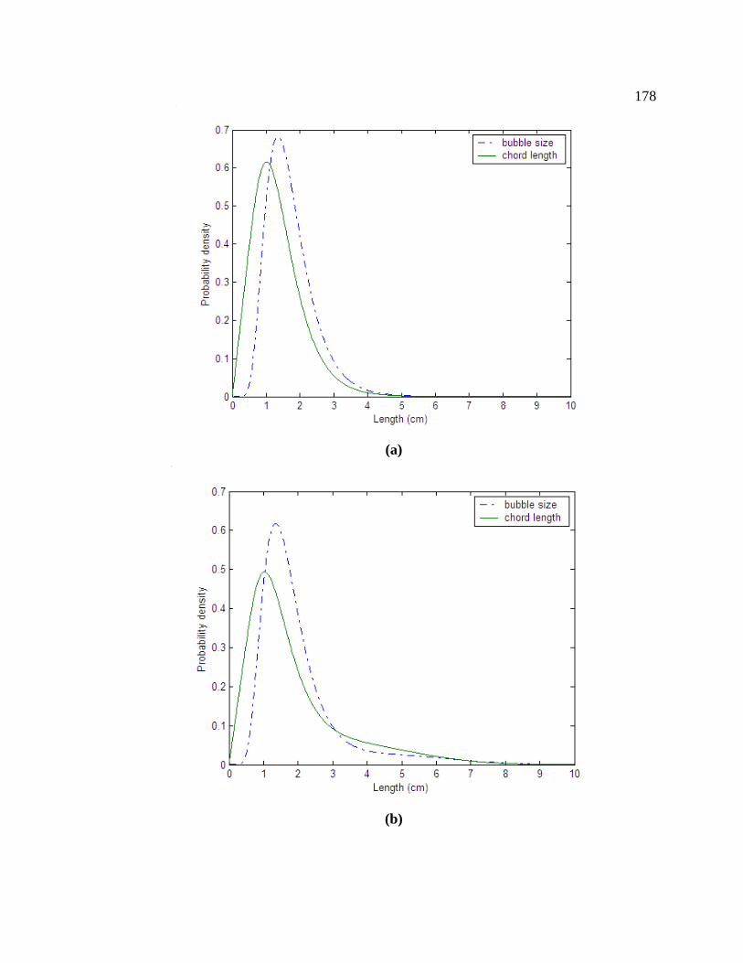
178

(a)

(b)

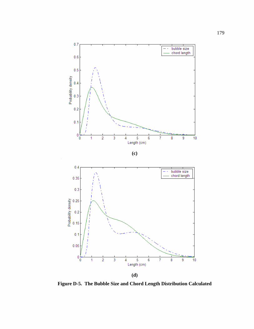
179

(c)

(d)

Figure D-5. The Bubble Size and Chord Length Distribution Calculated

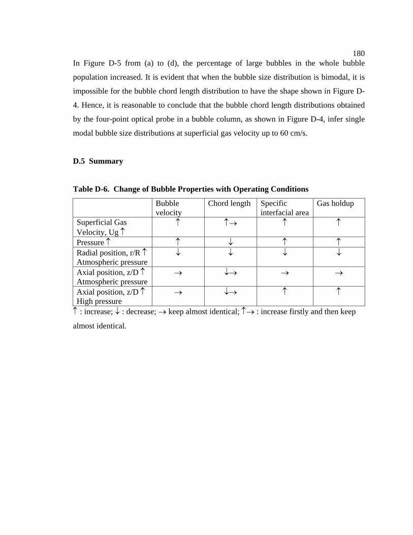
180In Figure D-5 from (a) to (d), the percentage of large bubbles in the whole bubble

population increased. It is evident that when the bubble size distribution is bimodal, it is

impossible for the bubble chord length distribution to have the shape shown in Figure D-

4. Hence, it is reasonable to conclude that the bubble chord length distributions obtained

by the four-point optical probe in a bubble column, as shown in Figure D-4, infer single

modal bubble size distributions at superficial gas velocity up to 60 cm/s.

D.5 Summary

Table D-6. Change of Bubble Properties with Operating Conditions

Bubble velocity

Chord length Specific interfacial area

Gas holdup

Superficial Gas Velocity, Ug ↑

↑ ↑→ ↑ ↑

Pressure ↑ ↑ ↓ ↑ ↑ Radial position, r/R ↑ Atmospheric pressure

↓ ↓ ↓ ↓

Axial position, z/D ↑ Atmospheric pressure

→ ↓→ → →

Axial position, z/D ↑ High pressure

→ ↓→ ↑ ↑

↑ : increase; ↓ : decrease; → keep almost identical; ↑→ : increase firstly and then keep

almost identical.

181

Appendix E Testing of Phase Transition At

Subcritical and Supercritical Conditions Using


The objective of this study is to evaluate the suitability of the four-point optical probe and

the algorithm for data processing in stirred autoclave reactors and minireactors (this work

was supported by the National Science Foundation Engineering Research Centers

Program, Grant EEC-0310689). In addition, the suitability of such probe to provide

transition information from two to single phase systems in expanded solvents will be

assessed. This information is necessary for evaluation of the medium and the selection of

the reactor type for the pilot plant and commercial implementation of the test bed reaction

systems under investigation.

The principle of the optical probe as explained in Section 3.2 makes it suitable for the

detection of the transition of the n-decane-CO2 system from two phases to one phase

(expanded solvent) with the increase in the pressure. The probe is going to be tested in a

1 liter autoclave stirred reactor (Figure E-1) using organic liquid (n-decane) with sparged

carbon dioxide. At subcritical condition, the CO2 will form bubbles in the n-decane phase

and these bubbles can be detected by the optical probe. At supercritical conditions, the

CO2 is miscible with organic solvent. Hence, there should be no bubbles detected. By this

means, the transition from two phases to expanded solvent (CO2 supercritical phase

systems) can be determined by the optical probe. The experimental conditions will be just

above the critical temperature of CO2 (31oC), e.g. 35oC. The operating pressure will be

0.1 to 10 MPa. Above 31oC and 7.28 MPa, the CO2 will be in supercritical condition.

Hence, 35oC and 0.1~10 MPa include the critical point of CO2.

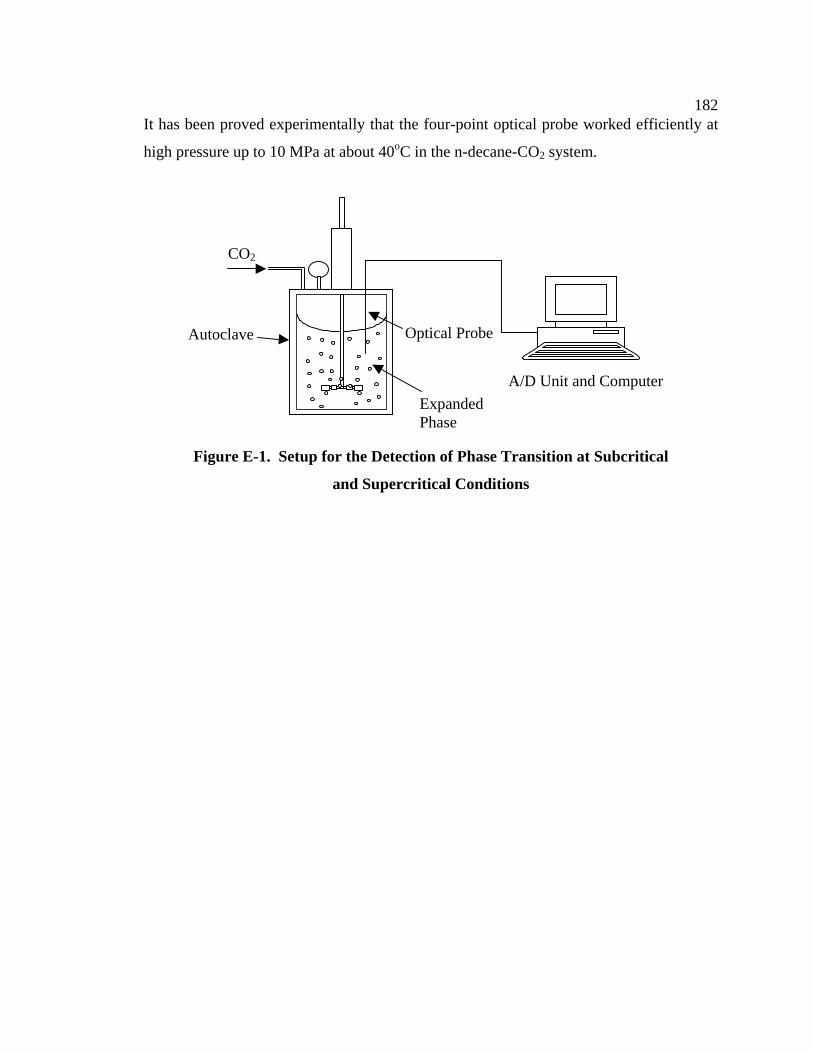
182It has been proved experimentally that the four-point optical probe worked efficiently at

high pressure up to 10 MPa at about 40oC in the n-decane-CO2 system.

Expanded Phase

CO2

Autoclave Optical Probe

A/D Unit and Computer

Figure E-1. Setup for the Detection of Phase Transition at Subcritical

and Supercritical Conditions

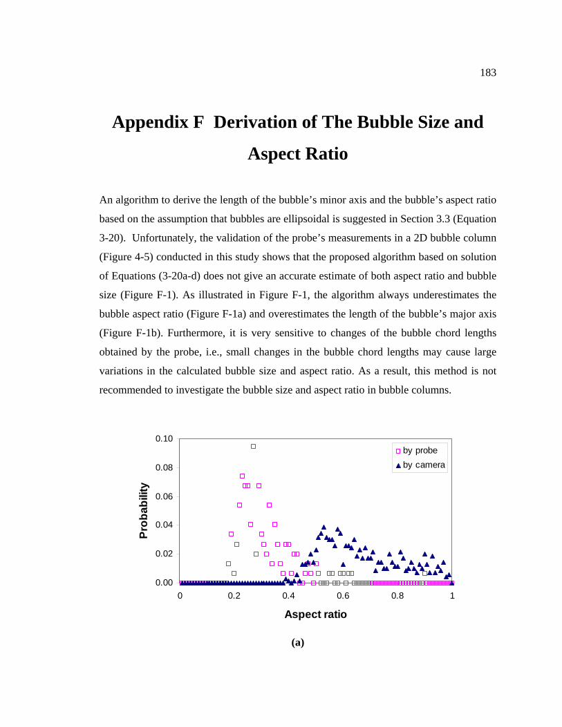
183

Appendix F Derivation of The Bubble Size and

Aspect Ratio

An algorithm to derive the length of the bubble’s minor axis and the bubble’s aspect ratio

based on the assumption that bubbles are ellipsoidal is suggested in Section 3.3 (Equation

3-20). Unfortunately, the validation of the probe’s measurements in a 2D bubble column

(Figure 4-5) conducted in this study shows that the proposed algorithm based on solution

of Equations (3-20a-d) does not give an accurate estimate of both aspect ratio and bubble

size (Figure F-1). As illustrated in Figure F-1, the algorithm always underestimates the

bubble aspect ratio (Figure F-1a) and overestimates the length of the bubble’s major axis

(Figure F-1b). Furthermore, it is very sensitive to changes of the bubble chord lengths

obtained by the probe, i.e., small changes in the bubble chord lengths may cause large

variations in the calculated bubble size and aspect ratio. As a result, this method is not

recommended to investigate the bubble size and aspect ratio in bubble columns.

0.00

0.02

0.04

0.06

0.08

0.10

0 0.2 0.4 0.6 0.8 1

Aspect ratio

Prob

abili

ty

by probeby camera

(a)

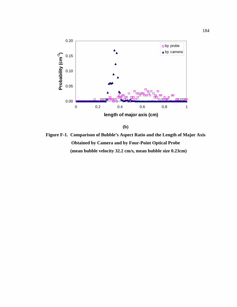
184

0.00

0.05

0.10

0.15

0.20

0 0.2 0.4 0.6 0.8 1

length of major axis (cm)

Prob

abili

ty (c

m-1

)

by probeby camera

(b)

Figure F-1. Comparison of Bubble’s Aspect Ratio and the Length of Major Axis

Obtained by Camera and by Four-Point Optical Probe

(mean bubble velocity 32.2 cm/s, mean bubble size 0.23cm)

185

References

1. Abuaf N., Jones O. C., Zimmer G. A. (1978). “Optical probe for local void fraction and interface velocity measurements”, Rev Sci Instrum, 49: 1090-1094

2. Akita K. and Yoshida F. (1973). “Gas holdup and volumetric mass transfer coefficient in bubble columns. Effect of liquid properties”, Ind Eng Chem Process Des Dev, 12: 76-80

3. Bach H. F. and Pilhofer T. (1978). “Variation of Gas Holdup in Bubble Columns with Physical Properties of Liquids and Operating Parameters of Columns”, Ger Chem Eng, 1:270

4. Batchelor G. K., “An introduction to fluid dynamics”, Cambridge U Press, London (1967), 474-481

5. Bhaga D., Weber M. E. (1981). “Bubbles in viscous liquids: shapes, wakes and velocities”, J Fluid Mech, 105: 61-85

6. Bruce C. A. (1985). “Probability and random processes: a first course with applications”, 2nd edition, J. Wiley, New York.

7. Burgess J. M., Calderbank P. H. (1975). “The measurement of bubble parameters in two-phase dispersions I: the development of an improved probe technique”, Chem Eng Sci, 30: 743-750

8. Cartellier A. (1998). “Measurement of gas phase characteristics using new monooptical fiber probes and real time signal processing”, Nucl Eng Des, 184: 393-408

9. Chabot J., Lee S. L. P., Soria A., De Lasa H. I. (1992). “Interaction Between Bubbles and Fiber Optic Probes in a Bubble Column”, Can J Chem Eng, 70: 61-68

10. Chanson H. (1997). “Air bubble entrainment in open channels: flow structure and bubble size distributions”, Int J Multiphase Flow, 23: 193-203

11. Chen J., Gupta P., Degaleesan S., Al-Dahhan M. H., Dudukovic M. P. and Toseland B. A. (1998). “Gas Holdup Distributions in Large-Diameter Bubble Columns Measured by Computed Tomography.” Flow Meas. Instrum., 9(2): 91-101

18612. Chen J., Li F., Degaleesan S., Gupta P., Al-Dahhan M. H., Dudukovic M. P. and

Toseland B. A. (1999a), “Fluid Dynamic Parameters in Bubble Columns with Internals.” Chem Eng Sci, 54: 2187-2197.

13. Chen J., Kemoun A., Al-Dahhan M. H., Dudukovic M. P., Lee D. J., Fan L-S. (1999b). “Comparative hydrodynamics study in a bubble column using computer-automated radioactive particle tracking (CARPT)/computed tomography (CT) and particle image velocimetry (PIV)”, Chem Eng Sci, 54: 2199-2207

14. Chen R. C., Reese J., Fan L-S. (1994). “Flow structure in a three-dimensional bubble column and three-phase fluidized bed”, AIChE J, 40: 1093

15. Choi K. H., Lee W. K. (1990). “Comparison of probe methods for measurement of bubble properties”, Chem Eng Comm, 91: 35-47

16. Clark N. N. and Turton R. (1988). “Chord length distribution related to bubble size distributions in multiphase flows”, Int J Multiphase Flow, 14: 413-424

17. Condon E. U., Odishaw H. (1967). “Handbook of physics”, 2 Ed., nd McGraw-Hill Book Co., New York.

18. Daly J. G., Patel S. A., Buckur D. B. (1992). “Measurement of gas holdups and Sauter mean bubble diameters in bubble column reactors by dynamic gas disengagement method”, Chem Eng Sci, 47(13-14): 3647-3654

19. Danckwerts P. V. (1970). “Gas-Liquid Reactions”, McGraw-Hill Book Co., New York.

20. Darton R. C., Harrison D. (1974). “The rise of single gas bubbles in liquid fluidized beds”, Trans I Chem E, 52: 301-306

21. Davis B. H. (2002). “Overview of reactors for liquid phase Fischer-Tropsch synthesis.” Catalysis Today, 71(3-4): 249-300

22. Deckwer W., Louisi Y., Zaidi A., Ralek M. (1980). “Hydrodynamic properties of the Fischer-Tropsch slurry process”, Ind Eng Chem Process Des Dev, 19: 699-708

23. De Lasa H. I., Lee S. L. P., Bergougnou M. A. (1984). “Bubble measurement in three-phase fluided beds using a U-shape optical fiber”, Can J Chem Eng, 62: 165-169

18724. De Swart J. W. A., Krishna R. (1995). “Effect of particles concentration on the

hydrodynamics of bubble column slurry reactors”, Chem Eng Res Design, Trans Ind Chem Eng, 73: 308-313

25. Deshpande N. S., Dinkar M., Joshi J. B. (1995). “Disengagement of the gas phase in bubble columns”, Int J Multiphase Flow, 21: 1191-1201

26. Domenico C., Damiano V., Roberto B., Maurizio M., Eiman Abu B. (1999). “A study on coalescence and breakage mechanisms in three different bubble columns”, Chem Eng Sci, 54: 4767-4777

27. Ellenberger, J. and Krishna, R. (1994). “A Unified Approach to the Scale-Up of Gas-Solid Fluidized Bed and Gas-Liquid Bubble Column Reactors”, Chem Eng Sci, 49: 5391-5411

28. Eisenberg B., Ansel L. L., Fiato R. A., Bauman R. F., “Advanced gas conversion technology for remote natural gas utilization”, GPA Convention, New Orleans, LA 1994

29. Fan L-S., Tsuchiya K., “Bubble wake dynamics in liquids and liquid-solid suspensions”, Butterworth-Heinemann, 1990

30. Fan L-S., Yang G. Q., Lee D. J., Tsuchiya K., Luo X. (1999), “Some aspects of high-pressure phenomena of bubbles in liquids and liquid-solid suspensions”, Chem Eng Sci, 54: 4681-4709

31. Farag H. I., Hjarbo K., Mejdell T., Hjarbo K., Ege P., Lysberg M., Grislingaas A., De Lasa H. I. (1997), “Fiber Optic and Capacitance Probes in Turbulent Fluidized Beds”, Chem Eng Comm, 157: 73-107

32. Frijlink J. J. (1987). “Physical aspects of gassed suspension reactors”, Ph. D. Thesis, Delft University of technology, the Netherlands.

33. Glassner A. S. (1990). “Graphics gems”, Academic Press, Boston.

34. Groen J. S., Oldeman R. G. C., Mudde R. F., van der Akker H. E. A., “Coherent structures and axial dispersion in bubble column reactors”, Chem Eng Sci, 51(1996): 2511-2520

35. Grunn D. J., Al-Doori H. H. (1985). “The measurements of bubbles flows in fluidized beds by electrical probe”, Int J Multiphase Flow, 11: 535-551

18836. Guet S., Fortunati R. V., Mudde R. F., Ooms G. (2003). “Bubble velocity and size

measurement with a four-point optical fiber probe’, Part Part Syst Charact, 20(2003): 219-230

37. Haberman W. L., Morton R. K. (1953). “An experimental investigation of the drag and shape of air bubbles rising in various liquids”, David W. Taylor Model Basin Report 802, Navy Dept., Washington DC

38. Harmathy, T. Z. (1960), “Velocity of large drops and bubbles in media of infinite or restricted extent”, AIChE J, 6: 281-288

39. Heijnen J. J., Van't Riet K. (1984), “Mass transfer, mixing and heat transfer phenomena in low viscosity bubble column reactors”, Chemical Engineering Journal (Amsterdam, Netherlands), 28(2): B21-B42

40. Hibiki T., Ishii M. (2002). “Interfacial Area Concentration of Bubbly Flow Systems” , Chem Eng Sci, 57: 3967-3977

41. Hibino S., “The behavior of single bubbles”, in Advances in Chemical Engineering 3: Dynamics of bubbles and Drops (Soc Chem Eng Japan, eds.), Chap. 2, 3-26, Nikkan Kogyo Shinbun, Tokyo, Japan 1969

42. Hills, J. H.; Darton, R. C. (1976). “The rising velocity of a large bubble in a bubble swarm”, Trans Inst Chem Eng, 54(4): 258-264

43. Hikita H., Asai S., Tanigawa K., Segawa K., Kitao M. (1980), “Gas hold-up in bubble columns”, Chemical Engineering Journal (Amsterdam, Netherlands), 20(1): 59-67

44. Hsu S. H., Lee W. H., Yang Y. M., Chang C. H. and Maa J. R. (2000). “Bubble Formation at an Orifice in Surfactant Solutions Under Constant-Flow Conditions”, Ind Eng Chem Res, 39: 1473-1479

45. Idogawa K., Ikeda K., Fukuda T. and Morooka S. (1987). “Formation and Flow of Gas Bubbles in a Pressurized Bubble Column with a Single Orifice or Nozzle Gas Distributor”, Chem Eng Comm, 59: 201-212

46. Idogawa K. (1997). “Methods for measurement of gas hold-up and gas bubble diameter in a high-pressure bubble column”, Kagaku Kogaku, 61: 781-782

18947. Iguchi M., Nakatani T., Kawabata H. (1997). “Development of a multineedle

electroresistivity probe for measuring bubble characteristics in molten metal baths”, Metallurgical and Materials Transactions B, 28: 409-416

48. Jager B., Espinoza R. (1995). “Advances in low temperature Fisher-Tropsch synthesis”, Catal Today, 23(1): 17-28

49. Jamialahmadi M., Muller-Steinhagen H. (1993). “Effect of superficial gas velocity on bubble size, terminal bubble velocity and gas hold-up in bubble columns”, Dev Chem Eng Miner Process, 1: 16-31

50. Jiang P., Lin T-J., Luo X., Fan L-S. (1995). “Flow visualization of high pressure (21 MPa) bubble column: bubble characteristics”, Chem Eng Res Des, 73: 269-274

51. Joshi J. B., Veera U. P., Parasad C. V., Phanikkumar D. V., Deshphande N. S., Thakre S. S. and Thorad B. N. (1998). “Gas Holdup Structure in Bubble Column Reactors.” PINSA, 64A(4): 441-567

52. Kataoka I., Ishii M., Serizawa A. (1986). “Local formulation and measurements of interfacial area concentration in two-phase flow”, Int J Multiphase flow, 12(4): 505-529

53. Kemoun A., Cheng Ong B., Gupta P., Al-Dahhan M. H. and Dudukovic M. P. (2001). “Gas Holdup in Bubble Columns at Elevated Pressure Via Computed Tomography”, Int J Multiphase Flow, 27(5), 929-946

54. Kiambi S. L., Duquenne A. M., Bascoul A. and Delmas H. (2001). “Measurements of local interfacial area: application of bi-optical fiber technique”, Chem Eng Sci, 56: 6447-6453

55. Kreischer B. E., Moritomi H., Fan L-S. (1990). “Wake solids holdup characteristics behind a single bubble in a three-dimensional liquid-solid fluidized bed”, Int J Multiphase Flow, 16: 187-200

56. Krishna R., Wilkinson P. M., van Dierendonck L. L. (1991). “A model for gas holdup in bubble columns incorporating the influence of gas density on flow regime transitions”, Chem Eng Sci, 46: 2491-2496

57. Kuncova G., Zahradnik J., Mach J. (1993). “Light Transmission Probe Connected with Spectrophotometer HP-8452 for local Measurements in Bubble Columns”, Chem Eng Sci, 48: 1013-1018

19058. Kulkarni A. A., Joshi J. B., Kumar V. R., Kulkarni B. D. (2001). “Simultaneous

Measurement of Holdup Profiles and Interfacial Area Using LDA in Bubble Columns: Predictions by Multiresolution Analysis and Comparison with Experiments”, Chem Eng Sci, 56: 6437-6445

59. LaNauze, R. D. and Harris, I. J., (1974). “Gas Bubble Formation at Elevated System Pressures”, Trans Instn Chem Engrs, 52(4): 337-348

60. Lans R. G. J. M. van der, van der Lans, R. G. J. M., “Hydrodynamics of a bubble column loop reactor”, Doctoral dissertation, Delft University of Technology, 1985.

61. Lee S. L., De Lasa H. I., Bergougnou M. A. (1986). “A U-shape fiber optic probe to study three-phase fluidized beds”, Part Sci Technol, 4: 61-71

62. Lee S. L., Soria A., De Lasa H. I. (1990). “Evolution of bubble length distributions in three phase fluidized beds”, AIChE J, 36: 1763-1767

63. Leibson, I., Holcomb, E. G., Cacoso, A. G., and Jacmic, J. J. (1956). “Rate of Flow and Mechanics of Bubble Formation from Single Submerged Orifices”, AIChE J, 2 (3): 296-306

64. Letzel H. M., Schouten J. C., Krishna R., van den Bleek C. M. (1997). “Characterization of regimes and regime transitions in bubble columns by chaos analysis of pressure signals”, Chem Eng Sci, 52: 4447-4459

65. Lim K. S., Agarwal P. K. (1992). “Bubble velocity in fluidized beds: the effect of non-vertical bubble rise on its measurement using submersible probes and its relationship with bubble size”, Powder Technology, 69: 239-248

66. Lin T-J., Tsuchiya K., Fan L-S. (1998). “Bubble flow characteristics in bubble columns at elevated pressure and temperature”, AIChE J, 44: 545-560

67. Lin T. J., Juang R. C., Chen Y. C., Chen C. C. (2001). “Predictions of flow transitions in a bubble column by chaotic time series analysis of pressure fluctuation signals. ” Chem Eng Sci, 56(3): 1057-1065

68. Liu W., Clark N. N., Karamavruc A. I. (1996). “General method for the transformation of Chord-length data to a local bubble-size distribution”, AIChE J, 42: 2713-2720

19169. Liu W., Clark N. N., Karamavruc A. I. (1998). “Relationship between bubble size

distribution and Chord-length distribution in heterogeneously bubbling systems”, Chem Eng Sci, 53: 1267-1276

70. Luewisutthichat W., Tsutsumi A., Yoshida K. (1997a). “Bubble characteristics in multi-phase flow systems: bubble sizes and size distribution”, J Chem Eng Jpn, 30: 461-466

71. Luewisutthichat W., Tsutsumi A., Yoshida K. (1997b), “Chaotic hydrodynamics of continuous single-bubble flow systems”, Chem Eng Sci, 52: 3685-3691

72. Luo X., Yang G., Lee D. J., Fan L-S. (1998). “Single bubble formation in high pressure liquid-solid suspensions”, Powder Technol, 100: 103-112

73. Manabu I., Hirotoshi K., Keiji N., Zen-Ichiro M. (1995). “Measurement of bubble characteristics in a molten iron bath at 1600°C using an electroresistivity probe”, Metall Mater Trans B, 26B: 67-74

74. Marques J. J. P., Bouard R. (1999). “Bubbles in a gas-solid fluidized bed. Photographic characterization”, Tech Mod, 91: 20-24

75. Matsuura A., Fan L-S. (1984). “Distribution of bubble properities in a gas-liquid-solid fluized bed”, AIChE J, 30: 894-903

76. Mihai M., Pincovschi I. (1998). “Experimental study of bubble size distribution in a bubble column”, Sci Technol Environ Prot, 5: 34-41

77. Mikkilineni S., Knickle H. N., “The effect of gas distributors on holdup and flow pattern in bubble columns”, Part. Multiphase Processes, [Proc. Int. Symp. Workshop] (1987), Meeting Date 1985, Publisher: Hemisphere, Washington D C, 3: 127-145

78. Miyahara T., Hamanaka H., Takino T., Akagi Y., Okada K. (1997). “Gas holdup, gas-liquid interfacial area and mass transfer coefficient in external-loop airlift bubble column containing low density particles”, J Chem Eng Japan, 30: 958-961

79. Mudde R. F., Bakker R. A., van der Akker H. E. A. (1992). “Noise analysis of transmitted light beams for determining bubble velocity and gas holdup profiles in a bubble column”, Chem Eng Sci, 47: 3631-3638

80. Mudde R. F., Saito T. (2001). “Hydrodynamical similarities between bubble column and bubbly pipe flow”, J Fluid Mech, 437: 203-228

19281. Olmos E., Gentric C., Vial Ch., Wild G., Midoux N. (2001). “Numerical simulation

of multiphase flow in bubble column reactors. Influence of bubble coalescence and break-up.” Chem Eng Sci, 56(21-22): 6359-6365

82. Ong, Boon Cheng (2003). “Experimental Investigation of Bubble Column Hydrodynamics: Effect of Elevated Pressure and Superficial Gas Velocity”, Ph. D. Thesis, Washington University in Saint Louis.

83. Patel S. A., Daly J. G., Bukur D. B. (1990). “Bubble-size distribution in Fischer-Tropsch-derived waxes in a bubble column”, AIChE J, 36: 93-105

84. Rajarathinam P., Nafis A. (1996). “Size distribution of bubbles generated by fine-pore spargers”, J Chem Eng Jpn, 29: 1030-1034

85. Reuter H. (1966). “The nature of bubbles in gas- and liquid-fluidized beds”, Chem Eng Progr Symp Ser, 62: 92-99

86. Rowe P. N., Widmer A. J. (1973). “Variation in shape with size of bubbles in fluidized beds”, Chem Eng Sci, 28(3): 980-981

87. Saberi S., Shakourzadeh K., Bastoul D., Militzer J. (1995). “Bubble Size and Velocity measurement in Gas-Liquid Systems: Application of Fiber Optic Technique to Pilot Plant Scale”, Can J Chem Eng, 73: 253-257

88. Saito T., Mudde R. F. (2001). “Performance of 4-tip optical fiber probe and bubble characterizations by the probe in turbulent bubbly flow”, ICMF2001

89. Sanaullah K., Zaidi S. H., Hills J. H. (2001). “A study of bubbly flow using resistivity probes in a novel configuration”, Chem Eng J, 83: 45-53

90. Saxena A. C., Rao N. S., Saxena, S. C. (1990). “Bubble Size Distribution in Bubble Columns”, Can J Chem Eng, 68: 159-161

91. Shollenberger K. A., Torczynski J. R., Adkins D. R., O’Hem T. J., Jackson N. B. (1997). “Gamma-densitometry tomography of gas holdup spatial distribution in industrial scale bubble columns”, Chem Eng Sci, 52: 2037-2048

92. Shollenberger K. A., Torczynski J. R., George, D. L. (2002). “Gas distribution in air/water and air/oil bubble-column flows”, FED (American Society of Mechanical Engineers) [257-2] (A, Proceedings of the 2002 ASME Joint U.S.-European Fluids Engineering Conference), 641-648

19393. Snabre P. and Magnifotcham F. (1998). “I. Formation and Rise of a Bubble Stream

in a Viscous Liquid”, Eur Phys J B, 4: 369-377

94. Spicka P., Martins A., Dias Madalena M., Lopes Jose Carlos B. (1999). “Hydrodynamics of gas-liquid flow in 2D packed/unpacked rectangular reactor”, Chem Eng Sci, 54: 5127-5137

95. Stegeman D., Knop P. A., Wijnands A. J. G., Westertern K. R. (1996). “Interfacial area and gas holdup in a bubble column reactor at elevated pressures”, Ind Eng Chem Res, 35: 3842-3847

96. Tang C., Heindel T. J. (2004). “Time-dependent gas holdup variation in an air-water bubble column”, Chem Eng Sci, 59: 623-632

97. Tadaki T. and Maeda S. (1963). “Size of bubbles from perforated plates”, Kagaku Kogaku, 27(6): 402-406

98. Terasaka K, Hieda Y. and Tsuge H. (1999). “SO2 Bubble Formation from an Orifice Submerged in Water”, J Chem Eng Japan, 32(4): 472-479

99. Tsuge H. and Hibino S. (1983). “Bubble Formation From An Orifice Submerged In Liquids”, Chem Eng Comm, 22: 63-79

100. Tsuge H., Nakajima Y. and Terasaka K. (1992). “Behavior of Bubbles Formed from a Submerged Orifice Under High System Pressure”, Chem Eng Sc., 47(13/14): 3273-3280

101. Vazquez G., Cancela M. A., Riverol C., Alvarez E. and Navaza J. M. (2000). “Determination of Interfacial Areas in a Bubble Column by Different Chemical Methods”, Ind Eng Chem Res, 39: 2541-2547

102. Vince M. A., Breed H., Krycuk G. and Lahey R.T. Jr. (1982). “Optical probe for high-temperature local void fraction determination”, Applied Optics, 21: 886-892

103. Wallis, G. B. (1969). “One-Dimensional Two-Phase Flow”, McGraw Hill, New York.

104. Wilkinson P. M. and van Dierendonck L. L. (1990). “Comments on Studies on Gas Holdup in a Bubble Column Operated at Elevated Temperatures”, Ind Eng Chem Res, 29: 927

194105. Wilkinson P. M., Haringa H. (1994), “Mass transfer and bubble size in a bubble

column under pressure”, Chem Eng Sci, 49: 1417-1427

106. Wu Q., Ishii M. (1999). “Sensitivity study on double-sensor conductivity probe for the measurement of interfacial area concentration in bubbly flow”, Int J Multi Flow, 25: 155-173

107. Xue J., Al-Dahhan M., Dudukovic M. P. (2003), Mudde R. F. “Bubble Dynamics measurements using Four-Point Optical Probe”, Canadian Journal of Chemical Engineering, 81: 375-381

108. Yang G. Q., Luo X., Lau R., Fan L-S. (2000). “Heat-transfer characteristics in slurry bubble columns at elevated pressures and temperatures”, Ind Eng Chem Res, 39: 2568-2577

109. Yoo D. H., Terasaka K. and Tsuge H. (1998). “Behavior of Bubble Formation at Elevated Pressure”, J Chem Eng Japan, 31(1): 76-82

110. Yu Y. H., Kim S. D. (1988). “Bubble Characteristics in the Radial Direction of the Three-Phase Fluidized Beds”, AIChE J, 34: 2069-2077

111. Zou R., Jiang X., Li B., Zu Y. and Zhang L. (1988). “Studies on Gas Holdup in a Bubble Column Operated at Elevated Temperatures”, Ind Eng Chem Res, 27:1910

bubble velocity, size and interfacial area measurements in bubble columns

Documents