Bubbles and crowding-in of capital via a savings glut

by Marten Hillebrand, Tomoo Kikuchi, Masaya Sakuragawa

No. 48 | NOVEMBER 2013

WORKING PAPER SERIES IN ECONOMICS

KIT – University of the State of Baden-Wuerttemberg andNational Laboratory of the Helmholtz Association econpapers.wiwi.kit.edu

Impressum

Karlsruher Institut für Technologie (KIT)

Fakultät für Wirtschaftswissenschaften

Institut für Volkswirtschaftslehre (ECON)

Schlossbezirk 12

76131 Karlsruhe

KIT – Universität des Landes Baden-Württemberg und

nationales Forschungszentrum in der Helmholtz-Gemeinschaft

Working Paper Series in Economics

No. 48, November 2013

ISSN 2190-9806

econpapers.wiwi.kit.edu

Bubbles and Crowding-in of Capital

via a Savings Glut∗

Marten Hillebrand†, Tomoo Kikuchi‡ and Masaya Sakuragawa§

November 18, 2013

Abstract

This paper uncovers a novel mechanism by which bubbles crowd in capital invest-

ment. If capital is initially depressed by a binding credit constraint, injecting a bubble

triggers a savings glut. Higher returns in a new bubbly equilibrium attract addi-

tional investors who expand investment at the extensive margin. We demonstrate

that crowding-in through this channel is a robust phenomenon that occurs along the

entire time path after bubbles are injected.

Keywords: Rational bubbles, savings glut, crowding-in, financial frictions

JEL Classifications: E21, E32, E44

1 Introduction

The US and other countries have experienced the dot-com bubble and real estate as well

as stock market booms since the late 1990s until the world plunged into recession in 2008.

∗We thank Costas Azariadis, Aditya Goenka, Christian Hellwig, Tomohiro Hirano, Basant Kapur, Mat-

suyama Kiminori, Noriyuki Yanagawa and Yan Zhang and seminar participants at Shanghai Jiao Tong,

Fudan and NUS for helpful comments and discussions. This research is supported by Grants-in-Aid for

Scientific Research (B) 22330062 from Japan Society for the Promotion of Science.†Department of Economics, Karlsruhe Institute of Technology. marten.hillebrand@kit.edu‡Department of Economics, National University of Singapore. ecstk@nus.edu.sg (Corresponding au-

thor)§Department of Economics, Keio University. masaya@econ.keio.ac.jp

1

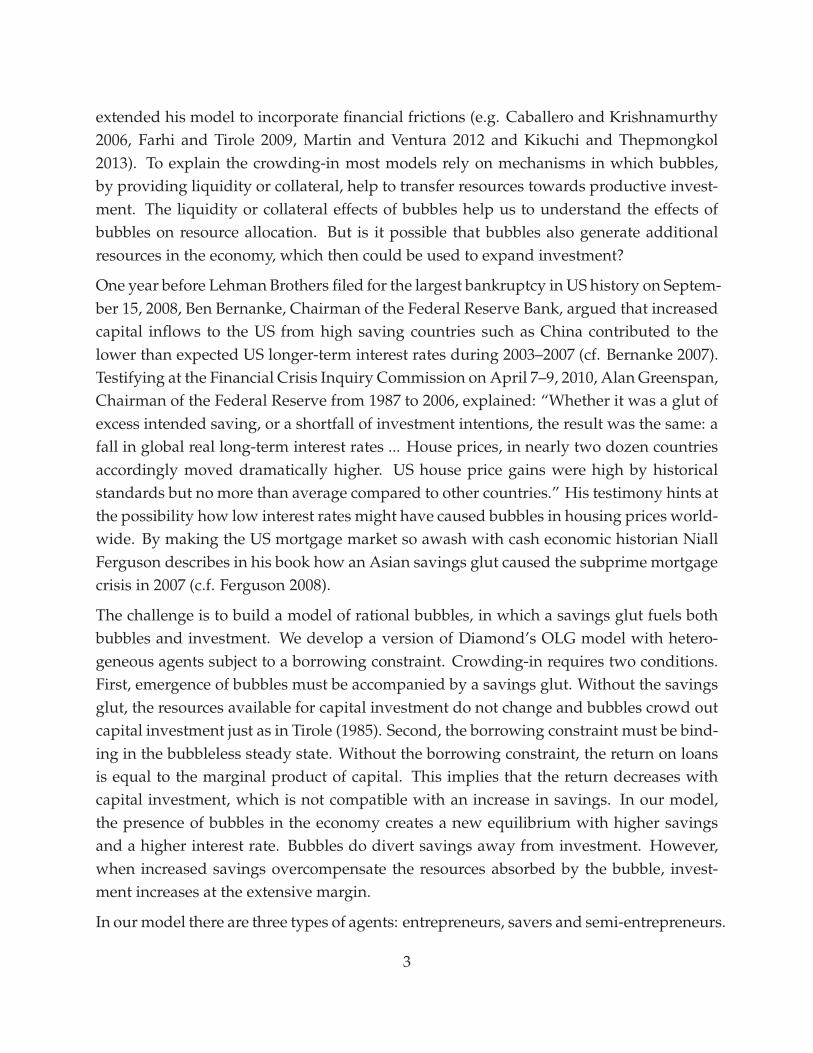
Figure 1 shows several interest rates and the average economic growth rate of G7 coun-

tries (Canada, France, Germany, Italy, Japan, the UK and the US).1 The interest rates are

greater than the economic growth rate except for the deposit rate until the end of the

1990s. The trend changes around 2000 when some interest rates drop below the growth

rate. After 2004 all interest rates are lower than the growth rate except for the lending rate

until 2008 when the bankruptcy of Lehman Brothers triggered a world-wide recession.

Note also that preceding the crisis, all the interest rates start to soar before they collapse.

-

-

GDP

Deposit

Bond

Money

Loan

2

2

4

4

6

1995 2000 2005

Figure 1: The interest rates and growth rate averaged over G7 countries

These observations seem to match the predictions by the theory of rational bubbles de-

veloped by Tirole (1985). The theory predicts that bubbles can arise as long as the growth

rate is above the interest rate in the steady state with no bubbles. By injecting a bub-

ble the economy converges to a steady state where the interest rate is higher. Where the

theory seems to be at odds with past episodes of bubbles is that bubbles crowd out cap-

ital because they compete with investment in capital in the portfolio of investors. Past

episodes of bubbles witnessed investment booms when they emerged (c.f. Kindeleberger

1996). Real estate bubbles in Japan in the late 1980s and in the US in the first decade of

21st century are recent major examples.

Under what conditions rational bubbles crowd in capital investment is a subject of great

importance in macroeconomics. Subsequent to Tirole’s (1985) analysis, the literature has

1Each of the interest rates and the economic growth rate is a simple average of G-7 countries (source:IFS).

We exclude the 1991 German data. The loan, bond, money and deposit are the call rate, the short-term rate

on the government bond, the short-term deposit interest rate, and the loan interest rate respectively.

2

extended his model to incorporate financial frictions (e.g. Caballero and Krishnamurthy

2006, Farhi and Tirole 2009, Martin and Ventura 2012 and Kikuchi and Thepmongkol

2013). To explain the crowding-in most models rely on mechanisms in which bubbles,

by providing liquidity or collateral, help to transfer resources towards productive invest-

ment. The liquidity or collateral effects of bubbles help us to understand the effects of

bubbles on resource allocation. But is it possible that bubbles also generate additional

resources in the economy, which then could be used to expand investment?

One year before Lehman Brothers filed for the largest bankruptcy in US history on Septem-

ber 15, 2008, Ben Bernanke, Chairman of the Federal Reserve Bank, argued that increased

capital inflows to the US from high saving countries such as China contributed to the

lower than expected US longer-term interest rates during 2003–2007 (cf. Bernanke 2007).

Testifying at the Financial Crisis Inquiry Commission on April 7–9, 2010, Alan Greenspan,

Chairman of the Federal Reserve from 1987 to 2006, explained: “Whether it was a glut of

excess intended saving, or a shortfall of investment intentions, the result was the same: a

fall in global real long-term interest rates ... House prices, in nearly two dozen countries

accordingly moved dramatically higher. US house price gains were high by historical

standards but no more than average compared to other countries.” His testimony hints at

the possibility how low interest rates might have caused bubbles in housing prices world-

wide. By making the US mortgage market so awash with cash economic historian Niall

Ferguson describes in his book how an Asian savings glut caused the subprime mortgage

crisis in 2007 (c.f. Ferguson 2008).

The challenge is to build a model of rational bubbles, in which a savings glut fuels both

bubbles and investment. We develop a version of Diamond’s OLG model with hetero-

geneous agents subject to a borrowing constraint. Crowding-in requires two conditions.

First, emergence of bubbles must be accompanied by a savings glut. Without the savings

glut, the resources available for capital investment do not change and bubbles crowd out

capital investment just as in Tirole (1985). Second, the borrowing constraint must be bind-

ing in the bubbleless steady state. Without the borrowing constraint, the return on loans

is equal to the marginal product of capital. This implies that the return decreases with

capital investment, which is not compatible with an increase in savings. In our model,

the presence of bubbles in the economy creates a new equilibrium with higher savings

and a higher interest rate. Bubbles do divert savings away from investment. However,

when increased savings overcompensate the resources absorbed by the bubble, invest-

ment increases at the extensive margin.

In our model there are three types of agents: entrepreneurs, savers and semi-entrepreneurs.

3

When a bubble appears, it competes with entrepreneurs for the economy’s savings rais-

ing the interest rate while lowering the entrepreneurial rate of return. The behavior of

entrepreneurs is not much affected by this change in rates of return as they only adjust

their capital investment at the intensive margin. Neither is the behavior of savers affected

as they just provide their entire labor income as loans. Semi-entrepreneurs, however,

start to save adding resources to the economy in response to the rise in the interest rate.

The increase in savings at the extensive margin (a savings glut) fuels bubbles while some

semi-entrepreneurs obtain access to capital investment and expand investment.

Who are the semi-entrepreneurs? Their savings are the only additional resources for in-

vestment in the economy. When they do not save, their wealth is consumed. Therefore,

we interpret the resources they provide as a savings glut, which is, strictly speaking, gen-

erated within the economy but may be viewed as an exogenous resource—more in line

with the story of the Asian savings glut. Whatever the interpretation, the key is that the

additional resources finance bubbles and expand investment.

The structure of the paper is as follows. Section 2 formulates the model and derives equi-

librium conditions. Section 3 uncovers the recursive structure of equilibria and defines a

state space. The existence of steady states and the scope for crowding-in are studied in

Section 4. The economic mechanism of the model are inspected in Section 5. Section 6

studies the dynamics. Section 7 concludes. All proofs can be found in the appendix.

2 The model

2.1 Production sector

The production sector consists of a single firm which operates a constant-returns-to-scale

technology to produce a consumable output good using capital and labor as inputs. The

production function in intensive form is f : R+ → R+ which is twice continuously dif-

ferentiable and satisfies f (0) = 0, f ′′ < 0 < f ′, limk↑∞ f ′(k) = 0 and limk↓0 f ′(k) = ∞.

At equilibrium labor supply will be constant and normalized to unity. Given the capital

stock kt > 0, perfect competition in factor markets determines the wage and capital return

in period t as

wt = f (kt)− kt f ′(kt) and t = f ′(kt). (1)

4

2.2 Heterogenous agents

In each period t ≥ 0, a continuum of young consumers is born whose mass is normalized

to unity. Each of these consumers lives for two periods and supplies one unit of labor in

the first period to earn labor income wt > 0. Each generation consists of three types of

consumers: (i) savers, (ii) entrepreneurs and (iii) semi-entrepreneurs.

Savers only consume in the second period of life and, therefore, wish to transfer their

current wealth wt into the next period. For this purpose, they supply loans to the credit

market and purchase bubbly assets whose value at time t is bt ≥ 0. Both investments

yield an identical return Rt+1 > 0.

Entrepreneurs have access to investment projects, which transform final goods into capital

unit by unit available in the next period. Entrepreneurs also consume only when old and,

therefore, invest their entire wealth when young. In addition, they take loans in the credit

market to finance their capital investment. The gross return earned by entrepreneurs on

their income wt is REt+1 ≥ Rt+1.

Semi-entrepreneurs have to decide whether to consume or save their wealth wt. When

they decide to save, they gain access to investment project just as an entrepreneur with

probability p ∈ (0, 1) and otherwise behave as a saver. The decision is irreversible and

made ex-ante, i.e., before the uncertainty is revealed.2 Thus, it must be based on the

ex-ante return

RSt+1 := pRE

t+1 + (1 − p)Rt+1. (2)

Semi-entrepreneurs save their wealth if and only if RSt+1 exceeds a threshold ρ > 0.

There are various interpretations for this assumption. First, ρ may represent an outside

investment opportunity (e.g., a foreign asset promising a return ρ). A second, alterna-

tive interpretation is that semi-entrepreneurs are endowed with a linear utility function

u(cy, c0) = cy + 1ρ c0 which would result in the same investment behavior. In what follows

we simply treat ρ as a parameter of the model.

2.3 Savings glut

The saving behavior of semi-entrepreneurs is the driving force of the model. Thus, with-

out loss of generality, the fractions of entrepreneurs and savers are assumed to be the

2Caballero and Krishnamurthy (2006) use a similar setup where investment opportunities are revealed

after saving decisions are made.

5

same and equal to a ∈ (0, 1/2). Defining s := 2a and s = 1, the saving decision by

semi-entrepreneurs determines the aggregate saving rate

st =

{s if RS

t+1 < ρ

s otherwise(3)

Equation (3) is precisely what we call a savings glut in our economy. It represents an ad-

justment of aggregate savings at the extensive margin, i.e., due to more people investing

if the return exceeds a certain threshold.

At the aggregate level, the total resources stwt invested in period t are used to form the

capital stock kt+1 of the following period and finance the current bubble bt. Thus,

kt+1 = stwt − bt. (4)

One observes from (4) that the savings boost (3) has the potential to explain crowding-in

of capital: If the injection of a bubble bt causes the savings rate st to increase from s to s,

this may overcompensate the resources absorbed by the bubble and capital may increase

relative to the bubbleless situation.

2.4 Investment behavior

Let αt denote the share of consumers who run investment projects at time t. These con-

sumers will be called investors. The behavior of semi-entrepreneurs determines the share

of investors as

αt =

{a RS

t+1 < ρ

a + p(1 − 2a) otherwise.(5)

Investors in period t take the wage wt and returns on capital f ′(kt+1) and loans Rt+1 as

given and choose investment i to maximize expected profit. The objective function reads

Πt+1(i) = f ′(kt+1)i − Rt+1(i − wt). (6)

In addition, we assume that investors can credibly pledge only a fraction λ ∈ (0, 1) of

expected earnings f ′(kt+1)i to meet their repayment obligation Rt+1(i − wt). Thus, the

choice of i is made subject to the borrowing constraint

Rt+1(i − wt) ≤ λ f ′(kt+1)i. (7)

The parameter λ can be interpreted as the degree of financial market imperfections, with

higher degree corresponding to a lower imperfection.3

3The simplest story to justify the assumption is that borrowers strategically default whenever the repay-

ment obligation exceeds the default cost, which is proportional to the project revenue.

6

2.5 Equilibrium

By (6), positive investment at equilibrium requires returns to satisfy the profitability con-

straint

Rt+1 ≤ f ′(kt+1). (8)

By (3) and (5), the share of consumers who behave as a saver can be written as st − αt.

Thus, the supply of loans is (st − αt)wt − bt and the demand for loans is αt(it − wt). This

and (4) determine equilibrium investment

it =stwt − bt

αt=

kt+1

αt. (9)

Using (9) in (7) determines the equilibrium borrowing constraint

Rt+1(kt+1 − αtwt) ≤ λ f ′(kt+1)kt+1. (10)

Perfect competition in the credit and capital markets implies that the return Rt+1 adjusts

until either the constraint (8) or (10) binds in equilibrium. Thus, given kt+1 determined

by (4) we obtain

Rt+1 =f ′(kt+1)

kt+1 − αtwtmin

{kt+1 − αtwt, λkt+1

}. (11)

Note that Rt+1 < f ′(kt+1) if the borrowing constraint (10) is binding. Also observe that

investors may invest part of their wealth in bubbles if the profitability constraint (8) is

binding. This happens precisely if it < wt, i.e., kt+1 < αtwt. Using (9) in (6) the return

earned by each entrepreneur is

REt+1 =

Πt+1(it)

wt=

f ′(kt+1)

αtwtmax

{αtwt, (1 − λ)kt+1

}. (12)

Note that if the borrowing constraint (10) is binding, REt+1 > f ′(kt+1) and semi-entrepreneurs

strictly prefer running projects to supplying credit or purchasing bubbles.

Young savers lend in the credit market at the return Rt+1 or purchase bubbles, which have

a fixed supply normalized to one, at price bt and sell them at price bt+1 in the next period.

Given the return determined by (11), no-arbitrage implies that the bubble evolves as

bt+1 = Rt+1bt. (13)

The economy can be summarized as E = (a, p, λ, ρ, f ) plus initial conditions k0 > 0 and

b0 ≥ 0. Following is a general definition of equilibrium.

Definition 2.1. Given k0 > 0 and b0 ≥ 0, an equilibrium of E is a sequence of non-

negative values {wt, bt, st, αt, kt+1, Rt+1, REt+1, RS

t+1}t≥0 which satisfies (1), (2), (3), (4), (5),

(11), (12) and (13) for all t ≥ 0.

7

3 Equilibrium dynamics

3.1 Recursive equilibrium structure

In this section, we uncover the forward-recursive structure of equilibria and formulate an

appropriate state space. Consider an arbitrary period t ≥ 0 and let the current bubble

bt ≥ 0 be determined by (13) and the capital stock kt > 0 determining the wage wt > 0

be given. In the following analysis, we will choose xt := (wt, bt) as our state variable

which takes values in some state space X to be specified below. While this is equivalent

to the usual choice (kt, bt), it will considerably simplify the results. In particular, several

equilibrium constraints and the stable manifold defined in Section 6.1 will become linear.

Given a candidate savings rate st ∈ {s, s}, the variables determined by (4), (5), (11), (12)

and (2) can be written as the following functions of the state variable xt:

kt+1 = K(xt; st) := stwt − bt (14a)

αt = α(st) := a + p(st − 2a) (14b)

Rt+1 = R(xt; st) :=f ′(kt+1)

kt+1 − αtwtmin

{kt+1 − αtwt, λkt+1

}(14c)

REt+1 = RE(xt; st) :=

f ′(kt+1)

αtwtmax

{αtwt, (1 − λ)kt+1

}(14d)

RSt+1 = RS(xt; st) := pRE(xt; st) + (1 − p)R(xt; st). (14e)

By (14a), positivity of capital requires bt < stwt, which imposes a first restriction on X. A

second restriction is that the savings rate st must be consistent with the savings behavior

of semi-entrepreneurs. For st = s, this requires RS(wt, bt; s) ≥ ρ while RS(wt, bt; s) < ρ

must hold for st = s to be consistent. Suppose that precisely one of these conditions holds.

Then, the consistent savings rate is determined by the mapping

S : X −→ {s, s}, st = S(xt) :=

{s if RS(xt; s) ≥ ρ

s if RS(xt; s) < ρ.(15)

Below we impose restrictions on X such that at least one of the two qualifications holds.4

Inserting (15) permits to write all variables determined by equations (14b–d) as functions

4For states where both s and s are consistent, the definition (15) would need to be modified to select a

savings rate, for example, by a random selection.

8

of xt alone. Furthermore, using (14b–d) and (15), the new state xt+1 = (wt+1, bt+1) is

determined as

wt+1 = Φ1(wt, bt) := W ◦K(wt, bt; S(wt, bt)) (16a)

bt+1 = Φ2(wt, bt) := btR(wt, bt; S(wt, bt)). (16b)

where W(k) := f (k) − k f ′(k). An initial state x0 ∈ X defines an equilibrium for E in the

sense of Definition 2.1 if (16,b) generates a sequence {xt}t≥0 of states which satisfy xt ∈ X

for all t ≥ 0. All other equilibrium variables follow from (14b–d) and (15).

3.2 Defining a state space

The set of states xt for which a continuation value xt+1 determined as in the previous

subsection is well-defined and decomposes into the set X of states consistent with high

savings st = s and the set X consistent with low savings st = s. Formally, recalling the

additional restriction bt < stwt

X :={(w, b) ∈ R

2+ | b < s w,RS(w, b; s) ≥ ρ

}(17a)

X :={(w, b) ∈ R

2+ | b < s w,RS(w, b; s) < ρ

}. (17b)

Defining the state space X := X∪X ensures that each xt ∈ X has a continuation value xt+1

which is unique whenever xt ∈ X\(X ∩ X). As mentioned in footnote 4, if X ∩ X 6= ∅,

the savings function (15) can be modified appropriately to induce a unique continua-

tion value. Also observe that for (16,b) to define a dynamical system, the mappings

Φ = (Φ1, Φ2) must further be restricted to a subset X ⊂ X which is self-supporting, i.e.,

Φ(X) ⊂ X. This is a typical property of models with bubbles also present—though not

explicitly discussed —in Tirole (1985). We will handle this issue in the following sections.

3.3 Regimes in the state space

The sets defined in (17a,b) can be partitioned into states where the borrowing constraint

is binding and where it is not. By (14c), the borrowing constraint is binding in period t, if

and only if kt+1 − αtwt > λkt+1. Using (14a), this is equivalent to bt < γ(st)wt where

γ(s) := s −α(s)

1 − λ, s ∈ {s, s}. (18)

9

We see that whether borrowing constraint binds in a given savings regime depends en-

tirely on the size of the ratio btwt

relative to a constant γ(s). As a consequence, the borrow-

ing constraint is more likely to bind if the bubble is small and vanishes if bt is large, rela-

tive to the wage wt. If bt is small, savings net of bubbles and thus investment are higher.

This implies a higher loans-to-investment ratio making the borrowing constraint more

likely to bind. In contrast, low savings net of bubbles decrease the loans-to-investment

ratio which relaxes the borrowing constraint. Also observe that γ(s) < s and, possibly,

γ(s) < 0. In the latter case, the borrowing will never bind.

Thus, we obtain four regions depending on whether savings are high or low and the

borrowing constraint is binding or not. Formally, X = XB ∪ XN and X = XB ∪ XN where

XB ={(w, b) ∈ X | b < γ(s)w

}, XB =

{(w, b) ∈ X | b < γ(s)w

}

XN ={(w, b) ∈ X | b ≥ γ(s)w

}, XN =

{(w, b) ∈ X | b ≥ γ(s)w

}.

(19)

We also let XB := XB ∪ XB and XN := XN ∪ XN the set of states where the borrowing

constraint is binding and where it is not.

4 Steady state analysis

In this section, we analyze steady states of Φ, i.e., states x ∈ X for which Φ(x) = x. We

call a steady state x = (w, b) bubbleless if b = 0 and bubbly otherwise. In what follows,

steady state values are denoted by the symbol of the respective variable with no time

index. In addition, a superscript zero identifies variables associated with a bubbleless

steady state.

4.1 Existence of steady states

To obtain explicit results and closed-form solutions, the remainder of this paper assumes

a Cobb-Douglas production technology f (k) := kθ , 0 < θ < 1. The economy is then sum-

marized by the list E = (a, p, λ, ρ, θ). Under this additional restriction, explicit conditions

can be derived under which steady states of either type (bubbleless or bubbly) exist in

the four regimes of the state space. These are stated formally in Lemma A.1 and A.2 in

Appendix A.1. The main findings are the following.

10

First, compared to similar models in the literature, additional restrictions are necessary

for steady states of either type to exist. These restrictions are necessary to render returns

consistent with the savings behavior of semi-entrepreneurs. Furthermore, Lemma A.2

shows that the returns supporting the bubbleless steady state are crucial for the existence

of bubbly steady states, a typical feature of OLG models with bubbles (cf. Tirole 1985 or

Kunieda 2008). As in these models, a bubble return less than unity is necessary to ensure

existence of a bubbly steady state in the same savings regime (if a bubbleless steady state

in the respective regime fails to exist, one should interpret the condition as a shadow

return). While these conditions are also sufficient in Tirole (1985) in the absence and

in Kunieda (2008) in the presence of financial frictions, more is required here to ensure

consistency with the savings behavior of semi-entrepreneurs. Section 5 offers a detailed

discussion of these conditions.

Second, both types of steady states may not be unique. However, if there are two bubble-

less steady states, either one will be in XB and the other one in XN or one will be in XN

and the other one in XB. Thus, in each of the sets XN , XB, X and X the map Φ possesses

at most one bubbleless steady state. The same holds for bubbly steady states. Again, the

potential multiplicity of steady states of each type—which is not observed in comparable

OLG models with bubbles—is due to the interaction between the financial friction and

the savings glut and vanishes as soon as one of these ingredients is turned off (cf. Section

5).

4.2 Crowding-in

Crowding-in occurs if capital or, equivalently, the wage in a bubbly steady state is higher

than in the bubbleless steady state. Formally, we have

Definition 4.1. Given a bubbleless steady state x0 = (w0, 0) and a bubbly steady state

x = (w, b), b > 0, we say that crowding-in occurs iff w > w0.

The following two results show that both the savings glut and the borrowing constraint

are essential for crowding-in. The economic intuition why this holds will be provided in

the next section.

Lemma 4.1. The following conditions are necessary for crowding-in:

(i) x0 ∈ X and x ∈ X (ii) x0 ∈ XB

11

Combining both results from Lemma 4.1, a necessary condition for crowding-in is that

x0 ∈ XB, i.e., the bubbleless steady state must lie in the low-savings regime and the bor-

rowing constraint must be binding at x0. Further, x must lie in the high-savings regime

X. It follows that we can distinguish the two cases where the borrowing constraint is

non-binding and binding at the bubbly steady state, i.e., x ∈ XN and x ∈ XB. The next

theorem provides a complete characterization for crowding-in to occur in each of these

two cases. Here we define for s ∈ {s, s} the functions

0(s) := θ1−θ

1s and B(s) := θ

1−θ1

α(s)+λ θ1−θ

. (20)

As shown in Appendix A.1, these mappings determine the capital returns in the bubble-

less steady state and in the bubbly steady state with a binding borrowing constraint.

Theorem 4.1. Let x0 = (w0, 0) ∈ XB and x = (w, b) ∈ X, b > 0 be steady states of Φ. Then,

crowding-in occurs iff either of the following conditions hold:

(i) x ∈ XN and 0(s) > 1 (ii) x ∈ XB and 0(s) > B(s).

As Theorem 4.1 is not stated in terms of the primitive parameters of the model, it raises the

questions whether the set of economies which satisfy either conditions (i) or (ii) of Theo-

rem 4.1 are non-empty and how they can be characterized. Let E := {E = (a, p, λ, ρ, θ) ∈

R5|0 < a <

12 , 0 < p < 1, 0 < λ < 1, ρ > 0, 0 < θ < 1} denote the entire class of

economies studied in this paper and E1 ⊂ E and E2 ⊂ E be the subclasses of economies

which satisfy conditions (i) and (ii) of Theorem 4.1. Then, E1 ∪E2 is the class of economies

for which crowding-in occurs. Note that E1 ∩ E2 = ∅.5 The following theorem comple-

ments Theorem 4.1 by providing a complete characterization of these classes.

Theorem 4.2. Both E1 and E2 are non-empty and take the following form:

E1 =

{(a, p, λ, ρ, θ) ∈ E

∣∣∣∣ λ <1

2, θ′ < 1, a <

θ′

2, θ′

π(λ; p)

a< ρ ≤ 1, θ′

1 − λ

π(a; p)< 1

}

E2 =

{(a, p, λ, ρ, θ) ∈ E

∣∣∣∣ λ <1

2, θ′

π(λ; p)

a< ρ ≤ 1 − p + pθ′

1 − λ

π(a; p),

2a < π(a; p) + λθ′ < min{

1, θ′}}

where π(x; p) := x(1 − p) + p(1 − x) and θ′ := θ1−θ .

12

0.0 0.1 0.2 0.3 0.4 0.5

0.0

0.1

0.2

0.3

0.4

0.5

p

λ

E1

E2

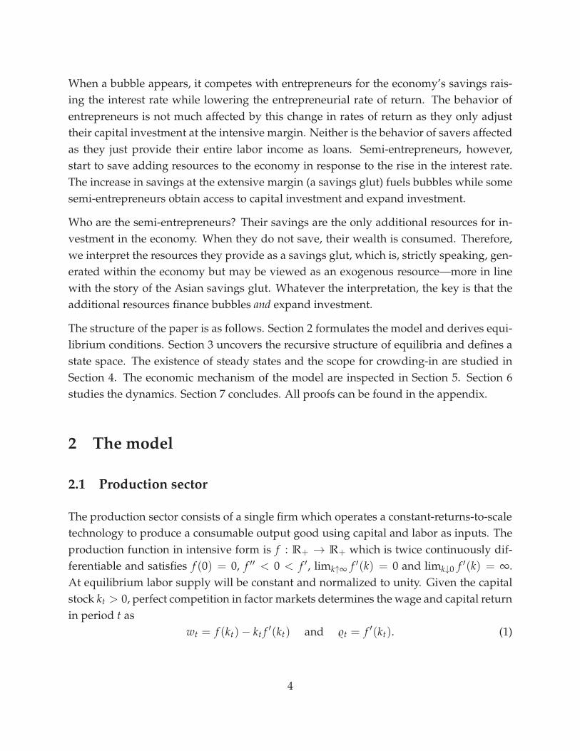
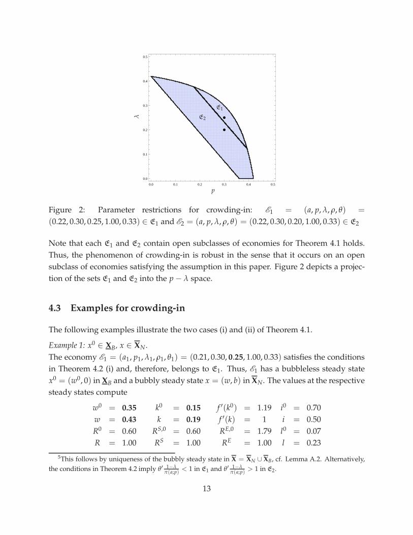
Figure 2: Parameter restrictions for crowding-in: E1 = (a, p, λ, ρ, θ) =

(0.22, 0.30, 0.25, 1.00, 0.33) ∈ E1 and E2 = (a, p, λ, ρ, θ) = (0.22, 0.30, 0.20, 1.00, 0.33) ∈ E2

Note that each E1 and E2 contain open subclasses of economies for Theorem 4.1 holds.

Thus, the phenomenon of crowding-in is robust in the sense that it occurs on an open

subclass of economies satisfying the assumption in this paper. Figure 2 depicts a projec-

tion of the sets E1 and E2 into the p − λ space.

4.3 Examples for crowding-in

The following examples illustrate the two cases (i) and (ii) of Theorem 4.1.

Example 1: x0 ∈ XB, x ∈ XN.

The economy E1 = (a1, p1, λ1, ρ1, θ1) = (0.21, 0.30, 0.25, 1.00, 0.33) satisfies the conditions

in Theorem 4.2 (i) and, therefore, belongs to E1. Thus, E1 has a bubbleless steady state

x0 = (w0, 0) in XB and a bubbly steady state x = (w, b) in XN. The values at the respective

steady states compute

w0 = 0.35 k0 = 0.15 f ′(k0) = 1.19 i0 = 0.70

w = 0.43 k = 0.19 f ′(k) = 1 i = 0.50

R0 = 0.60 RS,0 = 0.60 RE,0 = 1.79 l0 = 0.07

R = 1.00 RS = 1.00 RE = 1.00 l = 0.23

5This follows by uniqueness of the bubbly steady state in X = XN ∪ XB, cf. Lemma A.2. Alternatively,

the conditions in Theorem 4.2 imply θ′ 1−λπ(a;p)

< 1 in E1 and θ′ 1−λπ(a;p)

> 1 in E2.

13

Here, i0 = k0

α(s)and i = k

α(s)is the investment and l0 = α(s)(i0 − w0) and l = α(s)(i − w)

the credit volume at the respective steady states which we compute for later reference.

While in principle the economy could have an additional co-existing bubbleless steady

state x0 ∈ XN

and/or a bubbly steady state x ∈ XB, we readily check that neither the

conditions from Lemma A.1(i) nor from Lemma A.2(iv) are satisfied. Thus, the values

computed are in fact the only steady states of the economy. The bubble in this example

crowds in capital by 27%.

Example 2: x0 ∈ XB, x ∈ XB.

The economy E2 = (a2, p2, λ2, ρ2, θ2) = (0.21, 0.30, 0.20, 1.00, 0.33) satisfies the conditions

in Theorem 4.2 (ii) and, therefore, belongs to E2. Thus, E2 has a bubbleless steady state

x0 = (w0, 0) in XB and a bubbly steady state x = (w, b) in XB. The steady state values

compute

w0 = 0.35 k0 = 0.15 f ′(k0) = 1.90 i0 = 0.70

w = 0.38 k = 0.18 f ′(k) = 1.03 i = 0.47

R0 = 0.47 RS,0 = 0.90 RE,0 = 1.19 l0 = 0.07

R = 1.00 RS = 1.03 RE = 1.01 l = 0.28

Similar to the previous case, neither the conditions from Lemma A.1 (i) nor from Lemma

A.2 (ii) hold. Thus, the steady states computed are the only ones of the economy E2. The

bubble in this example crowds in capital by 20%.

In both of the previous examples the return earned by entrepreneurs decreases while the

one on loans rises. The final result of this section states that this result holds in general.

Proposition 4.1. Under crowding-in, the associated returns satisfy RE< RE,0 and R > R0.

When crowding-in occurs, savers will be better off since both the return on loans and

the wage increase. However, entrepreneurs will be better off only if the rise in the wage

overcompensate the decline in the return on investment. Both numerical examples show

that capital investment decreases at the intensive margin (i0> i) due to the decline in

the entrepreneurial return. However, the increase in investment at the extensive margin

overcompensates the decrease in investment at the intensive margin when bubbles crowd

in capital.

14

5 The mechanism

This section inspects the economic mechanisms of our model that generate crowding-in.

Recall that our model has two main ingredients: a financial friction and a savings glut. We

will first study each role separately by turning off the other mechanism and then show

how their interaction leads to crowding-in.

5.1 Role of the savings glut

We turn off the savings glut by assuming S(x) ≡ s for all x ∈ X. Formally, this can

be achieved by choosing ρ ∈ {0, ∞}. Then, by Lemmas A.1 and A.2, the economy E

has a unique bubbleless steady state x0 = (w0, 0) and at most one bubbly steady state

x = (w, b), b > 0. The bubbleless steady state lies in XB if γ(s) > 0 and in XN if γ(s) ≤ 0.

For ease of notation, define the functions

R0B(s) := θ

1−θλ

s−α(s), RE,0

B (s) := θ1−θ

1−λα(s)

, RS,0B (s) := pRE,0

B (s) + (1 − p)R0B(s). (21)

Note that all these mappings are strictly decreasing. As the notation suggests and shown

in Appendix A.1, they determine the returns at the bubbleless steady state with a binding

borrowing constraint. Lemma A.2 shows that they play a crucial role for existence of

bubbly steady states. There are two generic cases.

First, suppose RE,0B (s) < 1. In this case, the borrowing constraint will be non-binding

at any bubbly steady state (i.e., x ∈ XN provided it exists). A restriction necessary and

sufficient for x to exist is 0(s) < 1, which is precisely the overaccumulation condition

in Tirole (1985). As the bubbly steady state satisfies f ′(k) = 1 > f ′(k0), crowding-in is

excluded in this case. One may view the model as a special case of Tirole (1985) in this

first case.

Second, suppose RE,0B (s) > 1. In this case, the borrowing constraint will be binding at

the bubbly steady state (i.e., x ∈ XB provided it exists), but also at the bubbleless steady

state. In this case, a necessary and sufficient condition for x to exist is R0B(s) < 1, which

is precisely the existence condition in Kunieda (2008). Note that unlike the previous case,

the existence of a bubbly steady state is compatible with underaccumulation of capital at

the bubbleless steady state (i.e., f ′(k0) > 1). One may view our model as a special case of

Kunieda (2008) in this second case. As in his model, crowding-in is excluded.

15

Whether an initially binding borrowing constraint induces a spread between the returns

on capital and loans/bubbles or not, it does not affect the resources transferred through

the credit market because savers have a low (in fact, zero) intertemporal elasticity of sub-

stitution in consumption. Therefore, injecting a bubble necessarily absorbs part of con-

sumer incomes which unambiguously leads to crowding-out.6 This shows why savings

have to adjust at the extensive margin for crowding-in to occur.

5.2 Role of the financial friction

The financial friction can be turned off by setting λ = 1. In this case, by Lemmas A.1 and

A.2 the economy E has at most one bubbleless steady state x0 = (w0, 0) and at most one

bubbly steady state x = (w, b). Let us assume that both x0 and x exist.7

By the observations from the previous subsection, crowding-in can not occur if both

steady states lie in the same savings regime. Furthermore, the injection of bubbles can

only induce a switch from low to high savings (i.e., x0 ∈ X and x ∈ X). If the savings rate

is constant, any injection of bubbles crowds out investment. But then, returns—equal

to the marginal product of capital—would be higher in the bubbly equilibrium which is

inconsistent with a decline in savings rates.8

Therefore, suppose x0 ∈ X and x ∈ X, i.e., a savings glut occurs and investment adjusts at

the extensive margin. In the absence of the frictions, a savings glut is only compatible with

an increase in capital returns which requires a decrease in capital. Thus, the savings glut

alone is not sufficient to generate crowding-in. To summarize, the injection of bubbles is

capable of triggering the savings glut, but in the absence of financial frictions, this will

unambiguously lead to crowding-out.

6Formally, when the borrowing constraint is binding at the bubbly steady state f ′(k0) = 0(s) and

f ′(k) = B(s). The borrowing constraint is necessarily binding also at the bubbleless steady state. This and

R0B(s) < 1 imply 0(s) < B(s).

7Formally, by Lemma A.1, a bubbleless steady state exists in XN = X iff 0(s) ≥ ρ, in XN = X iff

0(s) < ρ and fails to exist if 0(s) < ρ ≤ 0(s). By Lemma A.2, a bubbly steady state exists in X iff

0(s) < 1 ∧ ρ ≤ 1 and in X iff 0(s) < 1 ∧ ρ > 1.8Note that by Lemma A.1 x0 ∈ X requires f ′(k0) = 0(s) ≥ ρ while x ∈ X requires ρ > 1 = f ′(k) and

0(s) < 1. But then, 0(s) > 0(s) which is impossible since 0 is decreasing.

16

5.3 Interaction of the financial friction and the savings glut

We saw in the previous subsections why crowding-in requires a switch from low to high

savings and a binding borrowing constraint in at least one of the two steady state. Let us

now assume 0 < ρ < ∞ and λ < 1 and focus on the case x0 ∈ X and x ∈ X.

Why does crowding-in require a binding borrowing constraint at the bubbleless steady

state? Suppose the borrowing constraint were non-binding at x0 (i.e., x0 ∈ XN). Then, as

demonstrated in the previous section, even if we were to switch to a bubbly steady state

x in the high-savings regime where the borrowing constraint is non-binding, crowding-

out necessarily occurs by savings consistency. If, in addition, capital is depressed at the

bubbly steady state due to a binding borrowing constraint, this would further amplify

and add to the crowding-out effect. Thus, x0 ∈ XN is not compatible with an increase in

returns necessary to support a savings glut. These insights show why savings must be

low and capital investment must be depressed due to a binding borrowing constraint at

the bubbleless steady state for crowding-in to occur.

We can now explain the mechanism of crowding-in. In the initial bubbleless steady state,

a binding borrowing constraint keeps the return on loans R0 low relative to the capital re-

turn. All capital investment is undertaken by entrepreneurs who earn a high return RE,0

while the return on bubbles R0 is still so low that RS,0< ρ and semi-entrepreneurs choose

not to save their wealth. Injecting a bubble now offers an alternative investment opportu-

nity to savers. In response they reduce their supply of loans—or demand a higher return

on their credit. This increases the returns R on loans and bubbles, and decreases the re-

turn RE earned by entrepreneurs. At this point, it is crucial that the change in returns

increases RS above the threshold value ρ to trigger a savings glut. For this to happen,

the probability p must be sufficiently small such that the increase in (1 − p)R overcom-

pensates the reduction in pRE. Instead of consuming semi-entrepreneurs now save and

invest their wealth which adds additional resources to the economy. Part of these addi-

tional resources is absorbed by the bubble while the rest increases the formation of capital.

Finally, recall that out of the group of semi-entrepreneurs, only a fraction p become in-

vestors while the remaining 1 − p become savers. Therefore, the additional formation of

capital is not necessarily accompanied by an increase in the resources exchanged through

the credit market. In fact, the numerical examples presented above demonstrate that the

equilibrium credit volume even decreases in the bubbly equilibrium (l < l0) making the

credit constraint less tight which may even vanish entirely.

17

6 Dynamics

We first provide a theoretical characterization of the stability properties of bubbleless and

bubbly steady states. We then focus on the crowding-in scenario and ask whether, starting

from a bubbleless situation, it is possible to inject a bubble to increase capital and converge

to the bubbly steady state. In the following analysis, we denote by Φn, n ≥ 0 the n-fold

composition Φ ◦ . . . ◦ Φ︸ ︷︷ ︸n-times

setting Φ0 = idX.

6.1 Stability of bubbleless steady states

Let X ∈ {XN, XB, XN, XB} be one of the four regimes defined above and x0 = (w0, 0) ∈ X

be a bubbleless steady state of the system (16,b). We define M0 to be the set of bubbleless

initial states attracted by x0—which stay in X under iteration of Φ and converge to x0.

Formally,

M0 :={(w, 0) ∈ X | Φ

n(w, 0) ∈ X ∀n ≥ 0 ∧ limn→∞

Φn(w, 0) = x0

}. (22)

Observe from (16) that for a given initial value w0 the bubbleless dynamics take the one-

dimensional form wt+1 = (1 − θ)(stwt)θ , t ≥ 0. Hence, for a constant savings rate s, any

initial value (w, 0) converges to x0 under iteration of Φ, even monotonically. Furthermore,

whether the borrowing constraint is binding or not is exclusively determined by whether

γ(s) > 0 or γ(s) < 0—whether it is binding at the steady state or not. Thus, it remains

to ensure that the savings rate is consistent with the returns along the entire path. We

obtain the following result which provides a complete characterization of the sets (22) for

each of the four cases from Lemma A.1. The proof follows from the respective savings

consistency condition and direct calculations.

Lemma 6.1. Let X ∈ {XN, XB, XN, XB} and x0 = (w0, 0) ∈ X be a steady state. Define

w0crit := w0(RS,0/ρ)

11−θ . Then, the following holds:

(i) If x0 ∈ X, then M0 = {(w, 0)|w ≤ w0crit}

(ii) If x0 ∈ X, then M0 = {(w, 0)|w > w0crit}

Note that in case (i) where x0 lies in the high savings regime, RS,0 ≥ ρ by savings-

consistency which implies w0crit ≥ w0. In this case, the steady state attracts all bubbleless

initial states which lie below the threshold w0crit. Likewise, w0

crit < w0 in case (ii) where

RS,0< ρ and the steady state attracts all initial states that exceed the threshold w0

crit.

18

6.2 Stability of bubbly steady states

Let X ∈ {XN, XB, XN , XB} be one of the four regimes defined above. We call a steady state

x ∈ X interior if x is an interior point of X. The stability properties of interior steady

states can be inferred by studying the Eigenvalues λ1, λ2 of the Jacobian matrix DΦ(x).

A steady state whose Eigenvalues are real and satisfy 0 ≤ |λ1| < 1 < |λ2| is called saddle-

path stable. In this case, stability obtains along a one-dimensional set M ⊂ X, the so-called

stable manifold. Formally,

M :={

x ∈ X | Φn(x) ∈ X ∀n ≥ 0 ∧ lim

n→∞Φ

n(x) = x}

. (23)

In other words, the stable manifold M associated with an interior steady state x ∈ X is

the set of points which remain in X under iteration of Φ and converge to x. As a major

advantage, our restriction to a Cobb-Douglas technology permits to characterize these

sets explicitly in the following result.

Lemma 6.2. Let X ∈ {XN, XB, XN, XB} and x = (w, b) ∈ X be an interior steady state. Then x

is saddle-path stable. Defining m := s(1− 0(s)f ′(k)

) and wcrit := w(RS/ρ)1

1−θ , the sets (23) take the

form:

(i) If x ∈ X, then M ={(w, b) ∈ R

2+ | w ≤ wcrit,

bw = m

}.

(ii) If x ∈ X, then M ={(w, b) ∈ R

2+ | w > wcrit,

bw = m

}.

Note that (w, b) ∈ M and that m > 0 as argued in footnote 9. Geometrically, M defines a

linear curve in the state space which is self-supporting under Φ (i.e., Φ(M) ⊂ M). Thus,

any initial state stays in M under iteration of Φ for all times t.

6.3 Multiple equilibria

The analysis from Section 4 revealed that two conditions must hold for crowding-in to

occur: 1. bubbles boost savings and 2. the borrowing constraint binds in the bubble-

less economy. Furthermore, the stability properties of steady states established that there

exists a saddle path M converging to the bubbly steady state and a bubbleless path M0

converging to the bubbleless steady state. We now limit our focus on the parameter set

for which crowding-in occurs and analyze the dynamics on a subset of the state space.

19

Let the economy E possesses a bubbleless steady state x0 = (w0, 0) ∈ XB and a bubbly

steady state x = (w, b) ∈ X. Assume that the hypotheses from Theorem 4.1(i) or (ii) are

satisfied such that w > w0. Suppose that the economy is initially in a bubbleless state with

a binding borrowing constraint (i.e., x0 = (w0, 0) ∈ XB). We now ask two questions. First,

is it possible to inject a bubble into the system such that long-run investment increases

and the economy converges to a bubbly steady state with higher capital? More formally:

Is there a value b0 > 0 which shifts the initial state x0 to x′0 = (w0, b0) such that the

economy converges to a bubbly steady state x? Second, which properties do we observe

along the path starting in x′0? The next theorem gives the answers.

Theorem 6.1. Let x0 = (w0, 0) ∈ XB and x = (w, b) ∈ X be steady states of (16,b) for which

w > w0. Then, we have:

(i) For all w0 < wcrit there is a unique b0 > 0 such that limt→∞ Φt(w0, b0) = x.

(ii) If w0 < w, the sequence (wt, bt) := Φt(w0, b0), t ≥ 0 is strictly increasing.

(iii) If w0 ≤ w0 < wcrit, then wt ≥ w0 for all times t ≥ 0.

The first assertion employs the explicit form of the stable set M from Lemma 6.2 and the

value b0 is such that x0 ∈ M. On M, convergence to x is always monotonic. By (ii), if the

initial state w0 is below w, the bubble increases investment immediately and in all future

periods relative to w0. In the case when w0 = w0, the economy is initially in a bubbleless

steady state, and crowding-in occurs immediately in t = 0 and investment continues to

increase in all successive periods as the economy converges to the bubbly steady state

x. Due to the stability properties of x0 stated in Lemma 6.1(ii), the assumption w0 = w0

seems not too restrictive. Finally, whether the bubbly steady state x satisfies the golden

rule depends on whether x ∈ XN or x ∈ XB. By Lemma A.2(i), the former is only possible

if ρ ≤ 1. The findings from Theorem 6.1 are illustrated in the following figure.

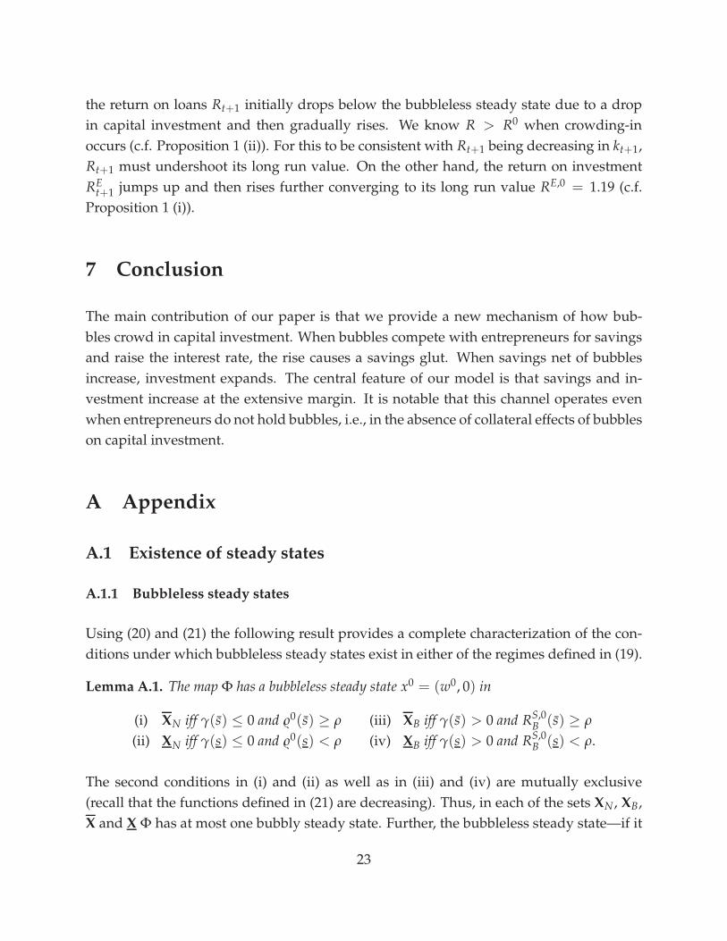
The remainder of this section illustrates the adjustment process towards the bubbly steady

state for the example economy E2 studied in Section 4.3. In the initial period t = 0, the

economy is in a bubbleless steady state x0 = (w0, 0) when a bubble b0 > 0 determined

as in Theorem 6.1 is injected into the system. Figure 4 shows the induced time series of

the bubble, the wage and the returns as the economy converges to the bubbly steady state

x = (w, b). The solid lines are the bubbleless steady state values. The dots show the

variables (bt, wt, Rt, REt ) in the bubbly equilibrium converging to (0.18, 0.38, 1.00, 1.01).

20

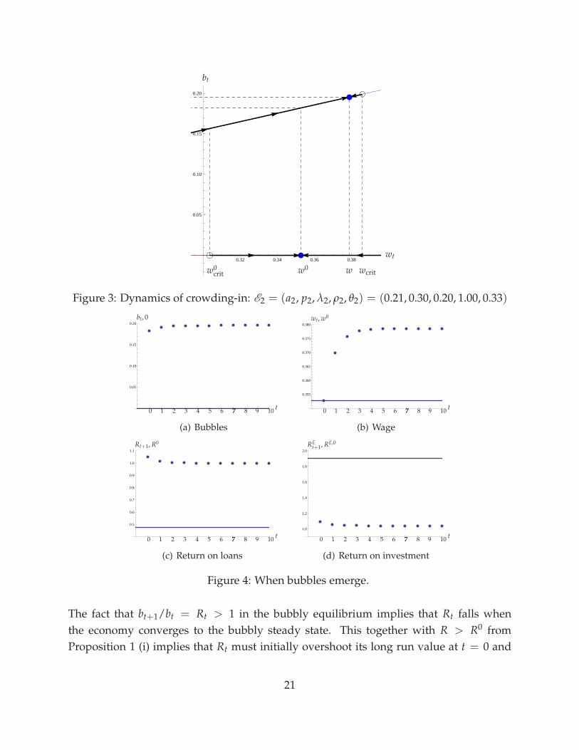
0.32 0.34 0.36 0.38

0.05

0.10

0.15

0.20

w0w0crit w wcrit

wt

bt

Figure 3: Dynamics of crowding-in: E2 = (a2, p2, λ2, ρ2, θ2) = (0.21, 0.30, 0.20, 1.00, 0.33)

0.05

0.10

0.15

0.20

t0 1 2 3 4 5 6 77 8 9 10

bt, 0

(a) Bubbles

0.355

0.360

0.365

0.370

0.375

0.380

t0 1 2 3 4 5 6 77 8 9 10

wt, w0

(b) Wage

0.5

0.6

0.7

0.8

0.9

1.0

1.1

t0 1 2 3 4 5 6 77 8 9 10

Rt+1, R0

(c) Return on loans

1.0

1.2

1.4

1.6

1.8

2.0

t0 1 2 3 4 5 6 77 8 9 10

REt+1, RE,0

(d) Return on investment

Figure 4: When bubbles emerge.

The fact that bt+1/bt = Rt > 1 in the bubbly equilibrium implies that Rt falls when

the economy converges to the bubbly steady state. This together with R > R0 from

Proposition 1 (i) implies that Rt must initially overshoot its long run value at t = 0 and

21

then decline. The injection of bubbles brings the economy on a new equilibrium where Rt

jumps initially due to an increase in investment at the extensive margin, which creates an

additional demand for credit. Savings also increase at the extensive margin. However, the

effect of savings net of bubbles is dominated by the demand effect when the interest rate

rises. When the borrowing constraint is binding, Rt+1 = λθkθt+1/(kt+1 − αtwt). Since Rt+1

is decreasing in kt+1, the overshooting must be caused by a jump in αt: an adjustment of

investment at the extensive margin. The jump in α, in contrast, causes REt+1 to fall. RE

t+1

drops and then must decline further to be consistent with RE,0> RE from Proposition

1 (ii). The fact that Rt+1 jumps up and REt+1 drops suggest that the probability p for

semi-entrepreneurs to obtain access to investment projects must be sufficiently low for a

savings glut to occur.

Figure 5 shows the time series in the bubbleless equilibrium starting at t = 0 with the

bubbly steady state value of the wage w = 0.35 as the initial condition. The solid lines are

the bubbly steady state values. The dots show the variables (bt, wt, Rt, REt ) in the bubbly

equilibrium converging to (0.00, 0.35, 0.47, 1.19).

0.05

0.10

0.15

0.20

t0 1 2 3 4 5 6 77 8 9 10

bt, 0

(a) Bubbles

0.355

0.360

0.365

0.370

0.375

0.380

t0 1 2 3 4 5 6 77 8 9 10

wt, w

(b) Wage

0.5

0.6

0.7

0.8

0.9

1.0

1.1

t0 1 2 3 4 5 6 77 8 9 10

Rt+1, R

(c) Return on loans

1.0

1.2

1.4

1.6

1.8

2.0

t0 1 2 3 4 5 6 77 8 9 10

REt+1, RE

(d) Return on investment

Figure 5: When bubbles burst.

Panel (a) simply shows the bubbly steady state value and zero. Panel (b) shows that

the wage gradually declines due to declining capital investment. Panel (c) shows that

22

the return on loans Rt+1 initially drops below the bubbleless steady state due to a drop

in capital investment and then gradually rises. We know R > R0 when crowding-in

occurs (c.f. Proposition 1 (ii)). For this to be consistent with Rt+1 being decreasing in kt+1,

Rt+1 must undershoot its long run value. On the other hand, the return on investment

REt+1 jumps up and then rises further converging to its long run value RE,0 = 1.19 (c.f.

Proposition 1 (i)).

7 Conclusion

The main contribution of our paper is that we provide a new mechanism of how bub-

bles crowd in capital investment. When bubbles compete with entrepreneurs for savings

and raise the interest rate, the rise causes a savings glut. When savings net of bubbles

increase, investment expands. The central feature of our model is that savings and in-

vestment increase at the extensive margin. It is notable that this channel operates even

when entrepreneurs do not hold bubbles, i.e., in the absence of collateral effects of bubbles

on capital investment.

A Appendix

A.1 Existence of steady states

A.1.1 Bubbleless steady states

Using (20) and (21) the following result provides a complete characterization of the con-

ditions under which bubbleless steady states exist in either of the regimes defined in (19).

Lemma A.1. The map Φ has a bubbleless steady state x0 = (w0, 0) in

(i) XN iff γ(s) ≤ 0 and 0(s) ≥ ρ (iii) XB iff γ(s) > 0 and RS,0B (s) ≥ ρ

(ii) XN iff γ(s) ≤ 0 and 0(s) < ρ (iv) XB iff γ(s) > 0 and RS,0B (s) < ρ.

The second conditions in (i) and (ii) as well as in (iii) and (iv) are mutually exclusive

(recall that the functions defined in (21) are decreasing). Thus, in each of the sets XN , XB,

X and X Φ has at most one bubbly steady state. Further, the bubbleless steady state—if it

23

exists—is unique if either γ(s) ≤ 0 ∧ γ(s) ≤ 0 or γ(s) ≥ 0 ∧ γ(s) ≥ 0. Thus, co-existing

bubbleless steady states can only occur if either γ(s) < 0 < γ(s) or γ(s) < 0 < γ(s), in

which case the borrowing constraint is binding in precisely one of them.

To characterize the associated steady state values, denote by s0 = S(x0) the savings rate

and k0 = K(x0; s0) the capital stock at the steady state x0. In cases (i) and (ii) of Lemma

A.1 where the borrowing constraint is non-binding, the steady state returns satisfy

R0 = RE,0 = RS,0 = f ′(k0) = 0(s0). (A.1)

In cases (iii) and (iv) where the borrowing constraint is binding, they are

R0 = R0B(s

0) < 0(s0) = f ′(k0) < RE,0 = RE,0B (s0), RS,0 = pRE,0 + (1 − p)R0. (A.2)

Note that f ′(k0) = 0(s0) independently of whether the borrowing constraint is binding

or not. Thus, the same holds for the steady state wage which can be written as

w0 = (1 − θ)θθ

1−θ 0(s0)−θ

1−θ . (A.3)

A.1.2 Bubbly steady states

The following result offers a complete characterization of the conditions under which

bubbly steady states exist in each of the four regimes defined in (19).

Lemma A.2. The map Φ has a bubbly steady state x = (w, b), b > 0 in

(i) XN, iff 0(s) < 1, RE,0B (s) < 1, and ρ ≤ 1

(ii) XN, iff 0(s) < 1, RE,0B (s) < 1, and ρ > 1

(iii) XB, iff R0B(s) < 1 < RE,0

B (s), and 1 − p + pRE,0B (s) ≥ ρ

(iv) XB, iff R0B(s) < 1 < RE,0

B (s), and 1 − p + pRE,0B (s) < ρ .

The last conditions (involving ρ) in cases (i) and (ii) as well as in (iii) and (iv) are again

mutually exclusive. The same is true of the requirements in (i) and (iii) as well as in (ii)

and (iv). Thus, in each of the sets XN , XB, X and X Φ has at most one bubbly steady state.

Of course, the existence conditions do not require a bubbleless steady state to exist in the

same regime.

24

To characterize the associated steady state values, denote by s = S(x) the savings rate

and by k = K(x; s) the capital stock at the bubbly steady state x. Then, the steady state

returns in cases (i) and (ii) satisfy

R = RS = RE = f ′(k) = 1. (A.4)

In cases (iii) and (iv) they are given by

R = 1 < f ′(k) = B(s) < RE = RE,0B (s) and RS = pRE + 1 − p. (A.5)

Using the previous definitions the steady state values can be expressed as9

w = (1 − θ)θθ

1−θ f ′(k)−θ

1−θ , b = sw

(1 −

0(s)

f ′(k)

). (A.6)

A.2 Proofs

Proof of Lemma A.1. As the question whether or not the borrowing constraint is binding

depends exclusively on the ratio bw (which is zero at any bubbleless steady state) rela-

tive to γ(s), the sign of the latter determines the regime in which the bubbleless steady

state lies. One can then show by direct computations using equations (14b)–(14e) that the

functions defined in (21) determine the steady state returns in the respective regime. The

second condition ensures consistency with the behavior of semi-entrepreneurs.

Proof of Lemma A.2. Define mt := btwt

. Then, using (16,b) and the Cobb-Douglas specifica-

tion, one obtains the following relation that holds for each t ≥ 0:

mt+1 = φ(mt; st) :=θ

1 − θ

mt

st − αt − mtmin

{λ,

st − αt − mt

st − mt

}. (A.7)

As the savings rate st = S(xt) can not be written as a function of mt, (A.7) does not

directly define a dynamical system in m. Observe, however, that for any bubbly steady

state x = (w, b) of Φ with steady state savings rate s = S(x), the ratio m := bw must be a

steady state of φ(·; s), i.e., m = φ(m; s) and 0 < m < s. In addition, the steady state returns

must be consistent with the behavior of semi-entrepreneurs. Evaluating these conditions

separately for each of the four regimes gives the conditions of the lemma.

9To see that the second quantity in (A.6) is positive, i.e.,0(s)f ′(k)

< 1 note that x ∈ XN implies f ′(k) = 1

and 0(s) < 1 by Lemma A.2(i),(ii) while x ∈ XB requires R0B(s) < 1 due to Lemma A.2(iii),(iv) which again

implies0(s)f ′(k)

= 0(s)B(s)

< 1. Thus, indeed b > 0. The economic reason is a crowding out effect that occurs

between the bubbleless and bubbly steady states that lie in the same savings regime.

25

Proof of Lemma 4.1. First note from (A.3), (A.6) that w > w0 iff f ′(k) < f ′(k0).

(i) Assume by contradiction that both x0 and x lie in X (the proof for X is analogous).

Suppose x ∈ XN. Then, f ′(k) < f ′(k0) iff 0(s) > 1, contradicting Lemma A.2(i). Suppose

x ∈ XB. Then, f ′(k) < f ′(k0) iff B(s) < 0(s), which can be rearranged to R0B(s) > 1,

contradicting Lemma A.2(iii).

(ii) By contradiction, let x0 ∈ XN . Then, by (i), x0 ∈ XN and f ′(k0) = 0(s). Suppose x =

(w, b) ∈ XN. Then, f ′(k) < f ′(k0) iff 0(s) > 1. But savings consistency requires f ′(k0) =

0(s) < ρ ≤ 1 = f ′(k) by Lemma A.1(ii) and Lemma A.2(i), which is a contradiction.

Second, suppose x ∈ XB. Then, f ′(k) < f ′(k0) iff

0(s) > B(s). (A.8)

The savings consistency conditions from Lemmas A.1(ii) and A.2(iii) yield

0(s) < ρ < 1 − p + pRE,0B (s). (A.9)

We also know from (A.5) that B(s) > 1. Thus, by (A.8) 0(s) > 1 and, therefore, 1 − p +

p0(s) < 0(s). Using this last result in (A.9) implies 0(s) < RE,0B (s). By Lemma A.1(ii)

γ(s) ≤ 0 which implies RE,0B (s) ≤ 0(s) by (21). Combining both results gives

RE,0B (s) ≤ 0(s) < RE,0

B (s)

which is impossible, since RE,0B defined in (21) is decreasing in s proving the claim.

Proof of Theorem 4.1. By (A.3) and (A.6), w > w0 iff f ′(k) < f ′(k0). Using (A.2) and (A.5)

gives precisely the conditions depending on whether x ∈ XN or x ∈ XB.

Proof of Theorem 4.2. Non-emptiness is a direct consequence of the examples. The condi-

tions stated can be verified directly by solving the parameter restrictions using the results

from Lemmas A.1 and A.2 and Theorem 4.1 together with equations (14b), (18), (20) and

(21).

Proof of Proposition 4.1. When bubbles crowd in investment, RE,0 = 1−λα(s)

θ1−θ > f ′(k0) > 1

and RE = max{1, 1−λα(s)

θ1−θ}. Hence, RE,0

> RE. From Lemma 3 (i), crowding-in requires a

savings glut. Hence, it must be that pRE + (1 − p)R > pRE,0 + (1 − p)R0 or (1 − p)(R −

R0) > p(RE,0 − RE). As RE,0> RE by the first part of this proof, R − R0

> 0.

26

Proof of Lemma 6.2. Let X be one of the four regimes. Evaluating the trace and determinant

of the Jacobian matrix DΦ(w, b) at the steady state one verifies that det DΦ(w, b) > 0 and

trDΦ(w, b) > 1 + det DΦ(w, b) > 0 which implies saddle-path stability. To explicitly

construct the stable sets (23), equation (A.7) is key. Let x0 = (w0, b0) ∈ M be arbitrary and

define xt := Φt(x0). As Φ(M) ⊂ M, xt ∈ M for all t ≥ 0. Further, M ⊂ X implies xt ∈ X

for all t ≥ 0, i.e., the sequence {xt}t≥0 stays in the same regime for all t ≥ 0. Therefore,

st = S(wt, bt) ≡ s for all t and the borrowing constraint is either always or never binding.

Define the induced sequence mt := btwt

, t ≥ 0 which necessarily satisfies mt < s for all

t ≥ 0. Given a constant savings rate s, (A.7) defines a one-dimensional dynamical system

which governs the evolution of (mt)t≥0. As limt→∞(wt, bt) = (w, b) by definition of M,

limt→∞ mt = m := bw where 0 < m < s. Consider the following two cases 1 and 2. In

case 1, X ⊂ XB and the borrowing constraint is always binding, i.e., mt < γ(s) for all

t ≥ 0. In case 2, X ⊂ XN and the borrowing constraint is never binding, i.e., mt ≥ γ(s)

for all t ≥ 0. In either case, (A.7) implies that the sequence (mt)t≥0 is generated by a

map of the form φ(m) = a0ma1−m , 0 < m < a1 where a0 = λ θ

1−θ , a1 = s − α(s) in case 1

while a0 = θ1−θ , a1 = s in case 2. One verifies directly that φ has precisely two steady

states m0 = 0 and m1 = a1 − a0. Note from Lemma A.2 that m1> 0 in both cases as

R0B(s) < 1 in case 1 and 0(s) < 1 in case 2. As φ′(m1) = 1 + m1/a0 > 1, m1 is unstable

while m0 is stable. By this observation , we claim that (w0, b0) must satisfy m0 = b0w0

= m1.

By contradiction, suppose m0 < m1. Then, stability of m0 implies limt→∞ mt = 0 which

contradicts limt→∞ mt = m. Conversely, suppose m0 > m1. Then, as limmրa1φ(m) = ∞,

the sequence {mt}t≥0 would grow without bound such that mt > a1 after finitely many

periods, which violates mt < γ(s) < a1 in case 1 and mt < s in case 2. Conclude that

indeed b0w0

= m1 which implies btwt

= m1 for all t ≥ 0 and, therefore, m = m1. It follows

that M is a subset of {(w, b) ∈ R2++|b = mw}. Also note that (A.4) and (A.5) permit m

to be written in the form stated in the lemma. Finally, bt = mwt and st ≡ s permit the

return (14e) earned by semi-entrepreneurs to be written as RSt+1 = f ′(kt+1)

f ′(k)RS =

(wtw

)θ−1RS

for each t ≥ 0. As the sequence {wt}t≥0 converges monotonically to w, the additional

conditions of the lemma restrict the initial value w0 such that RSt+1 ≥ ρ in case (i) and

RSt+1 < ρ in case (ii).

Proof of Theorem 6.1. The proof follows directly from Lemma 6.2 and the form of the stable

set M. Recall that Φ(M) ⊂ M such that (wt, bt) ∈ M and bt = mwt for all t ≥ 0. In

particular, wt+1 = (1 − θ)(s − m)θwθt for all t ≥ 0 which converges monotonically to

w.

27

References

[1] A. B. Abel, N. G. Mankiw, L. H. Summers, R. J. Zeckhauser, Assessing dynamic effi-

ciency: theory and evidence, Review of Economic Studies, 56 (1989) 1–20.

[2] B. S. Bernanke, Global imbalances: recent developments and prospects, Bundesbank

Lecture. Berlin, Germany, September 11, 2007.

[3] R. J. Caballero, A. Krishnamurthy, Bubbles and capital flow volatility: causes and risk

management, Journal of Monetary Economics, 53 (2006) 35–53.

[4] N. Ferguson, The ascent of money: a financial history of the world (New York: Pen-

guin Press, 2008).

[5] E. Farhi, J. Tirole, Bubbly liquidity, Review of Economic Studies, 79 (2009) 678–706.

[6] T. Kikuchi, A. Thepmongkol, Divergent bubbles in a small open economy, mimeo,

National University of Singapore, 2013.

[7] C. P. Kindleberger, Manias, panics, and crashes: A history of financial crises (London:

Macmillan, 1996).

[8] T. Kunieda, Asset bubbles and borrowing constraints, Journal of Mathematical Eco-

nomics, 44 (2008), 112–131.

[9] A. Martin, J. Ventura, Economic growth with bubbles, American Economic Review,

102 (2012) 3033–3058.

[10] K. Matsuyama, Financial market globalization, symmetry-breaking, and endoge-

nous inequality of nations, Econometrica 72 (2004) 853–884.

[11] J. Tirole, Asset bubbles and overlapping generations, Econometrica 53 (1985) 1499–

1528.

28

No. 48

No. 47

No. 46

No. 45

No. 44

No. 43

No. 42

No. 41

No. 40

No. 39

No. 38

Marten Hillebrand, Tomoo Kikuchi, Masaya Sakuragawa: Bubbles and

crowding-in of capital via a savings glut, November 2013

Dominik Rothenhäusler, Nikolaus Schweizer, Nora Szech: Institutions,

shared guilt, and moral transgression, October 2013

Marten Hillebrand: Uniqueness of Markov equilibrium in stochastic OLG

models with nonclassical production, November 2012

Philipp Schuster and Marliese Uhrig-Homburg: The term structure of

bond market liquidity conditional on the economic environment: an ana-

lysis of government guaranteed bonds, November 2012

Young Shin Kim, Rosella Giacometti, Svetlozar T. Rachev, Frank J. Fabozzi,

Domenico Mignacca: Measuring financial risk and portfolio optimization

with a non-Gaussian multivariate model, August 2012

Zuodong Lin, Svetlozar T. Rachev, Young Shin Kim, Frank J. Fabozzi:

Option pricing with regime switching tempered stable processes, August

2012

Siegfried K. Berninghaus, Werner Güth, Stephan Schosser: Backward

induction or forward reasoning? An experiment of stochastic alternating

offer bargaining, July 2012

Siegfried Berninghaus, Werner Güth, King King Li: Approximate truth of

perfectness - an experimental test, June 2012

Marten Hillebrand and Tomoo Kikuchi: A mechanism for booms and

busts in housing prices, May 2012

Antje Schimke: Entrepreneurial aging and employment growth in the

context of extreme growth events, May 2012

Antje Schimke, Nina Teichert, Ingrid Ott: Impact of local knowledge

endowment on employment growth in nanotechnology, February 2012

recent issues

Working Paper Series in Economics

The responsibility for the contents of the working papers rests with the author, not the Institute. Since working papers

are of a preliminary nature, it may be useful to contact the author of a particular working paper about results or ca-

veats before referring to, or quoting, a paper. Any comments on working papers should be sent directly to the author.