budgetary control · budgetary control 11.3 source: accounting: an introduction, 6/e, by peter...
TRANSCRIPT

11
BUDGETARY CONTROL
LEARNING OUTCOMES
After studying this chapter, you will be able to:
❑ Discuss the concept of the Budget as a Control System and the use of Responsibility Accounting
❑ Explain how Budgetary Systems fit within the Performance Hierarchy
❑ Select and Explain appropriate budgetary systems for an organisation, including Top-Down, Bottom-up, Feedback and Feed-forward Control
❑ Explain the Beyond Budgeting Model, including the benefits and problems that may be faced if it is adopted in an organisation
❑ Discuss the issues surrounding setting the difficulty level for a Budget
❑ Explain the benefits and difficulties of the Participation of Employees in the Negotiation of Targets
❑ Explain how Budget Systems can deal with uncertainty in the environment
© The Institute of Chartered Accountants of India
Merged By CA Study : Play Store App

11.2 STRATEGIC COST MANAGEMENT AND PERFORMANCE EVALUATION
CHAPTER OVERVIEW
BUDGETARY CONTROL
Budgetary Control is “Systematic control of an organization's operations through establishment of
standards and targets regarding income and expenditure, and a continuous monitoring and
adjustment of performance against them.”
Brown and Howard defines Budgetary Control is "a system of controlling costs which includes the
preparation of budgets, co-ordinating the departments and establishing responsibilities, comparing
actual performance with the budgeted and acting upon results to achieve maximum profitability. "
Budget is an estimation of revenues and expenses over a specified future period of time which
needs to be compiled and re-evaluated on a periodic basis based on the needs of the
organisation. Budgetary Control is the process by which budgets are prepared for the future
period and are compared with the actual performance for finding out variances, if any. In other
words, Budgetary Control is a process with the help of which, managers set financial and
performance goals, compare the actual results with the budgets, and adjust performance, as it is
needed.
Atrill and McLaney identify a number of characteristics that are common to businesses with
effective budgetary control:
© The Institute of Chartered Accountants of India
Merged By CA Study : Play Store App

BUDGETARY CONTROL 11.3
Source: Accounting: An Introduction, 6/E, By Peter Atrill, Eddie McLaney, David Harvey
Prerequisites of Effective Budgetary Control
A serious attitude to the system is required
Clear demarcation between areas of managerial responsibility
Reasonable budget targets
Established data collection, analysis and reporting techniques
Reports aimed at individual managers, rather than general
Fairly short reporting periods, typically a month
Timely variance reports
Action being taken to get operations back under control if they are shown
to be out of control
© The Institute of Chartered Accountants of India
Merged By CA Study : Play Store App

11.4 STRATEGIC COST MANAGEMENT AND PERFORMANCE EVALUATION
FEEDBACK AND FEED-FORWARD CONTROL
Feedback and Feed-forward are two types of control schemes for systems that react automatically
to changing environmental dynamics. Each utilizes sensors to measure important factors and a set
of rules to react to changes in those factors. Feedback and Feedforward Controls may coexist in
the same system, but the two designs function in very different ways.
Source: Management Accounting by Terry Lucey, Terence Lucey
Feedback Control
Feedback as the name suggests is a reaction after an action has taken place. So, there has to be
an error if we want to take corrective actions.
According to the CIMA’s Official Terminology, It is defined as: ‘Measurement of differences
between planned outputs and actual outputs achieved, and the modification of subsequent
action and/or plans to achieve future required results. Feedback control is an integral part of
budgetary control and standard costing systems.’
A feedback system would simply compare the actual historical results with the budgeted results.
© The Institute of Chartered Accountants of India
Merged By CA Study : Play Store App

BUDGETARY CONTROL 11.5
Types of Feedback
FeedbackPrimary
Could be reported to line management in the form of control reports, comparing actual and budgeted results.
If the variances are small or can be corrected easily then the information may not be feedback to anyone higher in the organisation.
SecondaryWhere feedback is sent to a higher level in an organisation and can lead to a plan being reviewed and possibly changed.
For example, the revision of a budget after large variances were discovered due to price changes over time.
NegativeFeedback taken to reverse a deviation from standard.
This could be by amending the inputs or process so that the system reverts to a steady state.
For example, a machine may need to be reset over time to its original settings.
PositiveTaken to reinforce a deviation from standard.
The inputs or process would not be altered.
© The Institute of Chartered Accountants of India
Merged By CA Study : Play Store App

11.6 STRATEGIC COST MANAGEMENT AND PERFORMANCE EVALUATION
Control Reports
Control reports are feedback devices, but they are only part of the feedback system. A control
report does not by itself cause a change in performance. A change results only when managers
take actions that lead to change1. Norton Bedford suggested the following five guidelines for
feedback management control reports2:
John C. Camillus suggested six broad approaches to implementing Preventive Management
Control2:
Feedback Management Control Report
Feedback report should disclose both
accomplishment and responsibility
Feedback reports should be extracted promptly
Feedback reports should disclose trends and
relationships
Feedback reports should disclose variations from
standards
Feedback reports should be in standardized
format
Indicator, both leading and
early warning
Contingency Plans
Trend Analysis
Adaptive Mechanisms
Congruent System Design
Policy Directives
© The Institute of Chartered Accountants of India
Merged By CA Study : Play Store App
BUDGETARY CONTROL 11.7
Limitations
Feedback control system does have some operational limitations. First, it depends heavily on
success of the error detection system. Second, there may be a time lag between the error
detection, error confirmation, and error revision during which actual results may change again 2.
Feed-forward Control
In certain cases, we may be able to measure the amount of error before it has actually taken
place. We may thus be able to place a control mechanism before the error takes place. Feed-
forward Control is one such Controlling system.
According to the CIMA’s Official Terminology, It is defined as the ‘forecasting of differences between actual and planned outcomes and the implementation of actions before the event, to avoid such differences.’
A feed-forward control system operates by comparing budgeted results against a forecast. Control
action is triggered by differences between budgeted and forecasted results.
Example
Information on Industrial Dispute in a state which was a major supplier of an important raw
material would cause smart buyers to buy before prices went up and their own inventory were
exhausted (in contrast a pure feedback system would not react until inventory had actually fallen).
Any manager who ignores feed-forward control will contribute to the downfall of a company.
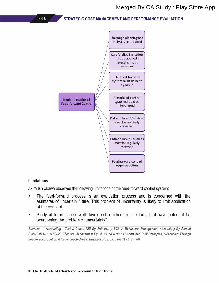
Implementation of Feed-forward Control3
Guidelines to be followed before implementation of Feed-forward Control
© The Institute of Chartered Accountants of India
Merged By CA Study : Play Store App
11.8 STRATEGIC COST MANAGEMENT AND PERFORMANCE EVALUATION
Limitations
Akira Ishiwkawa observed the following limitations of the feed-forward control system:
▪ The feed-forward process is an evaluation process and is concerned with the estimates of uncertain future. This problem of uncertainty is likely to limit application of the concept.
▪ Study of future is not well developed; neither are the tools that have potential fo r overcoming the problem of uncertainty2.
Sources: 1. Accounting - Text & Cases 12E By Anthony, p 803; 2. Behavioral Management Accounting By Ahmed
Riahi-Belkaoui, p 58-61; Effective Management By Chuck Williams (H Koontz and R W Bradspies, “Managing Through
Feedforward Control: A future directed view, Business Horizon, June 1972, 25-36).
Implementation of Feed-forward Control
Thorough planning and analysis are required
Careful discrimination must be applied in
selecting input variables
The feed-forward system must be kept
dynamic
A model of control system should be
developed
Data on Input Variables must be regularly
collected
Data on Input Variables must be regularly
assessed
Feedforward control requires action
© The Institute of Chartered Accountants of India
Merged By CA Study : Play Store App

BUDGETARY CONTROL 11.9
Case Scenario
Real Petroleum Corporation manufactures lubricant oils for motor vehicles (two wheelers, four
wheelers and heavy vehicles). The company offers lubricant oils in various packages ranging
from a 100 ml pouch to a 200 litres drum. About 70% of lubricant sales comprise are made in
the form of 900 ml ‘cans’. The process of manufacturing and packaging lubricant oils are given
below:
− Base oil of required grade is imported from middle east.
− The base oil is blended with additives at the manufacturing plants at specified
temperatures to produce lubricant oils.
− The oil is stored for a day to bring the temperature to normal.
− The plant has an automated bottling facility. The operator is required to pre-set the
quantity and number of ‘cans’ to be filled in a computerised system. No manual
intervention is required thereafter.
− The product is filled in ‘cans’ at the first stage of packaging with 900 ml of product.
− Caps are fixed on the ‘cans’ and sealed at the second stage of packaging.
− The product is weighed at third stage of packaging (a conversion factor is used to cover
volume into weight) before the ‘cans’ are packed into a carton.
Any ‘can’ having lesser quantity of oil is removed before the ‘cans’ are packed into the cartons.
The ‘cans’ which are short filled cannot be reused. Once the seal is broken, the ‘can’ is of no
use. There is no process by which the oil in short filled ‘can’ could be reused. Hence the
product is wasted.
The company is considering a proposal to add a component in its packaging unit to avoid
losses arising out of quantity issues in packaging. The component will be installed after the first
stage of packaging. The component will measure the volume of product and will forward the
‘can’ for capping and sealing only if the quantity in ‘cans’ is correct. In case the ‘can’ does not
have required volume of product, the ‘can’ will be topped up with balance product before the
capping and sealing process. The company will be able to achieve 0% wastage due to short
filling after implementation of new system.
Required
Using the context of control systems, IDENTIFY and EXPLAIN the type of control which is
existing in the company and the type of control which is proposed.
Solution
What is Control?
Control is a management function of establishing benchmarks and comparing actual
performance against the benchmarks and taking corrective actions. Control is required at all
levels of organisation to ensure that the organisation achieves its intended objective. There are
two types of control systems - Feedback Control and Feed-forward Control.
© The Institute of Chartered Accountants of India
Merged By CA Study : Play Store App

11.10 STRATEGIC COST MANAGEMENT AND PERFORMANCE EVALUATION
Feedback Control
Feedback Control is a control activity that takes place after a process is complete. It is also
known as post action control. If any problem is identified after a process i s complete, a
corrective action is taken to rectify the problem. Feedback control provides information only
after the process is complete and sometimes a significant time is lost to take corrective action.
Feedback-based systems have the advantage of being simple and easy to implement.
Real Petroleum currently has a feedback control mechanism in place. The actual volume of the
product is measured at the end of the packaging process. The current control process is that
any ‘can’ which is short filled is not packed in the carton. This ensures that a lower quantity of
product is not supplied into the market. The current control system, however leads to product
losses as identification of short-filled ‘cans’ at the end of process is not useful to the production
process. In case, there is a huge variation in the final packaging, the packaging system can be
reviewed to ensure that such problems do not acquire in the future.
Feed-forward Control
Feed-forward Control is also referred to as a preventive control. The rationale behind feed-
forward control is to foresee potential problems and take corrective action to ensure that the
final output is as expected. Feed-forward controls are desirable because they allow
management to prevent problems rather than having to cure them later. Feed-forward control
are costly to implement as it requires additional investment and resources. These are designed
to detect deviation some standard or goal to allow correction to be made before a particular
sequence of actions is completed
The proposed system in Real Petroleum is a Feed-forward control. In this case, any short filling
is identified in the packaging process itself and corrective action is taken to ensure that the final
packed ‘can’ has proper quantity of product. The new process is beneficial to the company as
the wastage arising out of the packaging process can be avoided. The savings must be
compared with the cost required to modify the packaging process before finalising on whether
the new system should be implemented or not.
BEHAVIOURAL ASPECTS OF BUDGETARY CONTROL
Behavioural aspects elucidate that many of the goals of budgeting are contradictory. On the one
side, we want to be able to fairly evaluate the performance of managers. But we also want to
motivate managers and therefore, even if managers are not involved in the process , managers
may find the budget too challenging and therefore reduce their effort. That in turn would distort any
evaluation. The participation of managers in setting targets for themselves tends to improve
motivation and performance. If, we want budgets to act as a way of communicating organisational
goals. But the budget themselves may distort the goals as they will be very short term, be focused
on cost reduction rather than, say, quality aspects, and they will solely focus on financial aspects
of the organisation's goals. There is therefore a conflict between aiming to achieve financial co ntrol
and communicating the organisation's goals.
© The Institute of Chartered Accountants of India
Merged By CA Study : Play Store App

BUDGETARY CONTROL 11.11
Moreover, the budget is framed to act as a plan for a manager, section, or division. The manager
may therefore pursue this plan at the cost of other critical success factors that emerge in the
internal or external environment of the firm. For example, a production manager may continue to
use the planned materials mix even if the sales department are indicating that customers would
desire a different product design and the purchasing department have accommodated their
purchases accordingly. The production manager then has to choose between the plan and inter
departmental coordination.
Many of the conflicts arise due to the human nature of a budgetary control system. Managers do
not always follow organisational goals, they do not always think long term, they may be cautious of
moving away from the plan etc. This provides a conflict between many of the goals of a budgetary
control system which needs to be considered at a strategic level when implementing such a
system.
Budget Slack
Budget affects the approach and behaviour of managers and used to motivate the managers.
Unrealistic demanding targets tend to affect manager’s performance adversely. Allowing
managers to set their own targets will introduce slack targets. Managers working in an
environment where they are expected to meet the budget targets often try to introduce slack
into budget. But, where there is more relaxed attitude, or when other factors are considered
alongside the analysis of variances, managers are general less inclined to introduce slack. But
it can have a detrimental impact on the evaluation of actual performance if managers
incorporate 'slack' into the budget in order to make it easier to achieve.
Effect of the Budget Difficulty on Performance
Once budgets have been set as performance targets, surely performance will be evaluated. This
can be simply a comparison of actual with budgeted performance or alternatively can be a more
detailed comparison of actual performance with flexed budget performance, as is found in variance
analysis and operating statements. The evaluation step is often one of the most argumentative as
it is here that performance is likely to be criticised and employees will be sensitive. There are
many potential difficulties:
Hofstede (1968)
▪ Budgets have no motivational effect unless they are accepted by the managers involved as their own personal targets.
▪ Up to the point where the budget is no longer accepted, the more demanding the target the better the results achieved.
▪ Demanding budgets are seen as more relevant than less difficult targets, but negative attitudes result if they are seen as too difficult.
▪ Acceptance of budgets is facilitated when good upward communication exists. The use of departmental meeting was found helpful in encouraging managers to accept budget targets .
© The Institute of Chartered Accountants of India
Merged By CA Study : Play Store App

11.12 STRATEGIC COST MANAGEMENT AND PERFORMANCE EVALUATION
▪ Managers’ reactions to budget targets were found affected both by their own personality and by more general cultural and organizational norms.
The relationship between budget difficulty and the ensuring level of performance can be shown
graphically and is illustrated as under:
The Effect of Budget Difficulty on Performance
Source: Otley (1987)
“Budget level that motivates the best level of performance may not be achievable. In contrast, the
budget that is expected to be achieved motivates a lower level of performance as managers no
longer aspire to meet the budget target.” The balanced scorecard approach of Kaplan and Norton,
and the building block approach of Fitzgerald and Norton can be a great help in ensuring that
objectives (or targets), or budgets are set for a very wide range of factors, both financial and non-
financial.
Case Scenario
“It's frustrating working with Denial. He’s very dominant and expects everything to be done his
way. We have done more and better work to get up to budget, and the minute we make it he
tightens the budget on us. We can’t work any faster and still maintain quality. We always see m
to be interrupting the big jobs for all those small rush orders. The accountants seem to know
everything that’s happening in my department, sometimes even before I do. I thought all that
budget and accounting stuff was supposed to help, but it just gets me into trouble. I’m trying to
put out quality work; they’re trying to save money. This is a dead-end job. I don't see much of a
future here.”
– said Mr. Singh, manager of the machine shop of Global Mfg. Ltd. a UK based Company.
Mr. Singh had just attended the monthly performance evaluation meeting for plant department heads. These meetings had been held on the third Friday of each month since Mr. Denial, MBA from Manchester University, had joined the Indian operations a year earl ier. Mr. Singh had just
© The Institute of Chartered Accountants of India
Merged By CA Study : Play Store App
BUDGETARY CONTROL 11.13
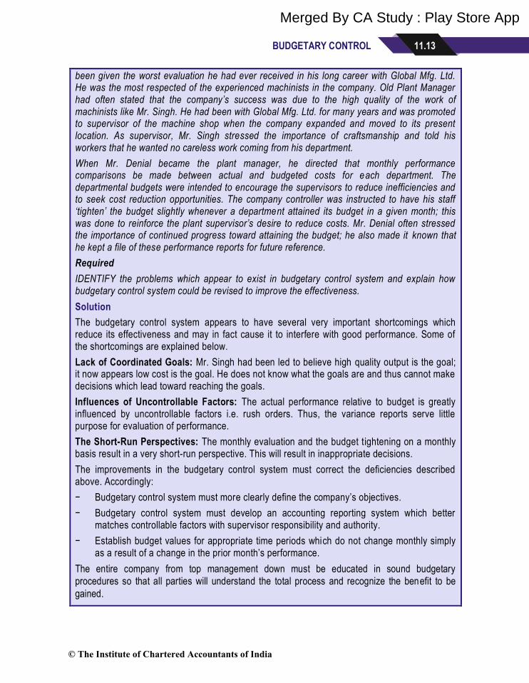
been given the worst evaluation he had ever received in his long career with Global Mfg. Ltd. He was the most respected of the experienced machinists in the company. Old Plant Manager had often stated that the company’s success was due to the high quality of the work of machinists like Mr. Singh. He had been with Global Mfg. Ltd. for many years and was promoted to supervisor of the machine shop when the company expanded and moved to its present location. As supervisor, Mr. Singh stressed the importance of craftsmanship and told his workers that he wanted no careless work coming from his department.
When Mr. Denial became the plant manager, he directed that monthly performance comparisons be made between actual and budgeted costs for each department. The departmental budgets were intended to encourage the supervisors to reduce inefficiencies and to seek cost reduction opportunities. The company controller was instructed to have his staff ‘tighten’ the budget slightly whenever a department attained its budget in a given month; this was done to reinforce the plant supervisor’s desire to reduce costs. Mr. Denial often stressed the importance of continued progress toward attaining the budget; he also made it known that he kept a file of these performance reports for future reference.
Required
IDENTIFY the problems which appear to exist in budgetary control system and explain how budgetary control system could be revised to improve the effectiveness.
Solution
The budgetary control system appears to have several very important shortcomings which reduce its effectiveness and may in fact cause it to interfere with good performance. Some of the shortcomings are explained below.
Lack of Coordinated Goals: Mr. Singh had been led to believe high quality output is the goal; it now appears low cost is the goal. He does not know what the goals are and thus cannot make decisions which lead toward reaching the goals.
Influences of Uncontrollable Factors: The actual performance relative to budget is greatly influenced by uncontrollable factors i.e. rush orders. Thus, the variance reports serve little purpose for evaluation of performance.
The Short-Run Perspectives: The monthly evaluation and the budget tightening on a monthly basis result in a very short-run perspective. This will result in inappropriate decisions.
The improvements in the budgetary control system must correct the deficiencies described above. Accordingly:
− Budgetary control system must more clearly define the company’s objectives.
− Budgetary control system must develop an accounting reporting system which better matches controllable factors with supervisor responsibility and authority.
− Establish budget values for appropriate time periods which do not change monthly simply as a result of a change in the prior month’s performance.
The entire company from top management down must be educated in sound budgetary
procedures so that all parties will understand the total process and recognize the benefit to be
gained.
© The Institute of Chartered Accountants of India
Merged By CA Study : Play Store App

11.14 STRATEGIC COST MANAGEMENT AND PERFORMANCE EVALUATION
Participation in Budget Setting Process
There are two main approaches to budgeting, the top down approach and bottom up approach.
Budgets can be prepared centrally and subordinates have little influence on the target setting. This
called top down budget or imposed style approach. The benefit of top down approach is that it
can be produced quickly and involve less management time than other options. However, there
are significant risk of inaccurate budgets being set that are also not acceptable to the subordinate
managers.
An alternative to top-down approach is for the subordinate managers to participate in the
preparation of their own budgets and then these budgets to be reviewed by senior management.
This is called bottom up approach (sometimes referred participative approach).
© The Institute of Chartered Accountants of India
Merged By CA Study : Play Store App

BUDGETARY CONTROL 11.15
Many researchers have recommended that the bottom up approach involving participation is a
preferable method of preparing a budget. Other studies have suggested that participation is not a
solution that will solve all problem. Following table highlights factors that have been suggested in
different studies as influencing the effectiveness of participation:
Study Factors Influencing the Effectiveness of Participation
Participation is Less Effective and Relevant
Vroom (1960) Personality With managers who are more highly authoritarian.
Hopwood (1978) Work Situation In a highly programmed and technologically constrained environment.
Brownell (1981) Locus of Control For those individuals who feel they have a low degree of control over their destiny.
Mia (1989) Job Difficulty Where job difficulty is low.
Bruns and Waterhouse (1975)
Types of Organizational Structure In a centralized organization.
Source: Business Planning and Control: Integrating Accounting, Strategy, and People by Bruce Bowhill
The testimony from the various research proposed that participative styles of management will not
necessarily more effective than other styles, and that participative methods should be used with
care. Accordingly, it is essential to identify those circumstances where there is testimony that
participative methods are effective, rather than to introduce universal application into firms.
Participation must be used selectively; but if it is used in the right circumstances, it has an
outstanding potential for encouraging the assurance to organisational goals, enlightening attitudes
towards budgeting system, and increasing subsequent performance. However, there are some
limitations on the positive effects of participation in standard setting and circumstances where top-
down budget setting is preferable1. They are as follows:
Where personality characteristics of the participation may limit the benefits of
participation
Where participation by itself is not adequate in ensuring commitment to
standards and managers can significantly influence the results
Where a process is highly programmable and clear, stable input-output
relationships
Where a firm has large number of homogeneous units and operating in a
stable environment
Circumstances Where Top-Down Budget
Setting is Preferable
© The Institute of Chartered Accountants of India
Merged By CA Study : Play Store App
11.16 STRATEGIC COST MANAGEMENT AND PERFORMANCE EVALUATION
Case Scenario
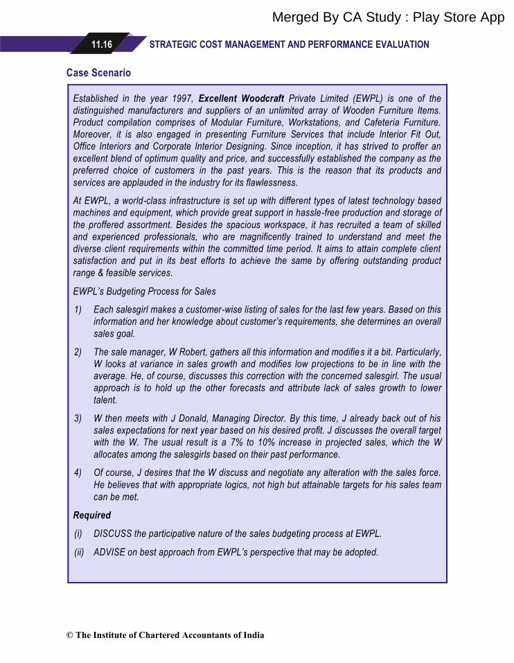
Established in the year 1997, Excellent Woodcraft Private Limited (EWPL) is one of the
distinguished manufacturers and suppliers of an unlimited array of Wooden Furniture Items.
Product compilation comprises of Modular Furniture, Workstations, and Cafeteria Furniture.
Moreover, it is also engaged in presenting Furniture Services that include Interior Fit Out,
Office Interiors and Corporate Interior Designing. Since inception, it has strived to proffer an
excellent blend of optimum quality and price, and successfully established the company as the
preferred choice of customers in the past years. This is the reason that its products and
services are applauded in the industry for its flawlessness.
At EWPL, a world-class infrastructure is set up with different types of latest technology based
machines and equipment, which provide great support in hassle-free production and storage of
the proffered assortment. Besides the spacious workspace, it has recruited a team of skilled
and experienced professionals, who are magnificently trained to understand and meet the
diverse client requirements within the committed time period. It aims to attain complete client
satisfaction and put in its best efforts to achieve the same by offering outstanding product
range & feasible services.
EWPL’s Budgeting Process for Sales
1) Each salesgirl makes a customer-wise listing of sales for the last few years. Based on this
information and her knowledge about customer’s requirements, she determines an overall
sales goal.
2) The sale manager, W Robert, gathers all this information and modifies it a bit. Particularly,
W looks at variance in sales growth and modifies low projections to be in line with the
average. He, of course, discusses this correction with the concerned salesgirl. The usual
approach is to hold up the other forecasts and attribute lack of sales growth to lower
talent.
3) W then meets with J Donald, Managing Director. By this time, J already back out of his
sales expectations for next year based on his desired profit. J discusses the overall target
with the W. The usual result is a 7% to 10% increase in projected sales, which the W
allocates among the salesgirls based on their past performance.
4) Of course, J desires that the W discuss and negotiate any alteration with the sales force.
He believes that with appropriate logics, not high but attainable targets for his sales team
can be met.
Required
(i) DISCUSS the participative nature of the sales budgeting process at EWPL.
(ii) ADVISE on best approach from EWPL’s perspective that may be adopted.
© The Institute of Chartered Accountants of India
Merged By CA Study : Play Store App

BUDGETARY CONTROL 11.17
Solution
(i) In participative budgeting, subordinate managers create their own budget and these budgets are reviewed by senior management. Such budget communicates a sense of responsibility to subordinate managers and fosters creativity. This is also called bottom up approach (sometime referred as participative approach).
As the subordinate manager creates the budget, it might be possible that the budget’s goals become the manager’s personal goal, resulting in greater goal congruence. In addition to the behavioural benefits, participative budgeting also has the advantage of involving individuals whose knowledge of local conditions may enhance the entire planning process.
The participative budget described here appears participative in name only. In virtually every instance, the participative input is subject to oversight and discussion by sales manager. Some amount of revision is also common. However, excessive and arbitrary review that substitutes a top-down target for a bottom-up estimate makes a deceit process. Such a gutting appears to be the case in EWPL. J’s statement indicates a very autocratic style. The revision process also seems to be arbitrary and capricious. There is little incentive for the salesgirls to spend much time and effort in projecting the true expected sales because they know that the target would be revised again and J’s estimate will prevail. This situation creates an interesting discussion about the costs and benefits of participative budgeting and gives rise to game playing and slack.
(ii) In top down approach, budget figures will be imposed on sales personnel by senior management and sales personnel will have a very little participation in the budget process. Such budget will not interest them since it ignores their involvement altogether. While in bottom up approach, each sales person will prepare their own budget. These budgets will be combined and reviewed by seniors with adjustment being made to coordinate the needs and goals of overall company. Proponents of this approach is that salespersons have the best information of customer ’s requirements, therefore they are in the best position in setting the sales goal of the company. More importantly, salespersons who have role in setting these goals are more motivated to achieve these goals. However, this approach is time-intensive and very costly when compared with top down approach. In order to achieve personal goals, participants may also engage in politics that create budgetary slack and other problems in the budget system.
Since both top down and bottom up approaches are legitimate approaches, so EWPL can use combination of both. Seniors know the strategic direction of the company and the important external factors that affect it , so they might prepare a set of planning guidelines for the salesgirls. These guidelines may include forecast of key economic variables and their potential impact on the EWPL, plans for introducing and advertising a new product and some broad sales targets etc. With these guidelines, salesgirls might prepare their individual budget. These budgets need to be reviewed to validate the uniformity with the EWPL’s objectives. After review, if changes are to be made, the same should be discussed with salesgirls involved.
© The Institute of Chartered Accountants of India
Merged By CA Study : Play Store App
11.18 STRATEGIC COST MANAGEMENT AND PERFORMANCE EVALUATION
Use of Accounting Information in Performance Evaluation1
Some dysfunctional consequences that arise with accounting measures of performance may not
be due to the insufficiency of the performance measures, but rather may outcome from the way in
which the accounting measures are used. The accounting information provided by an accounting
system must be interpreted and used with care.
Hofstede (1968) found that stress on the actual results in performance evaluation led to more
extensive use of budgetary information, and this made the budget more relevant. However, t his
stress was associated with a feeling that the performance appraisal was unjust. To overcome this
problem, the correct balance must be established when the budgeted performance is evaluated.
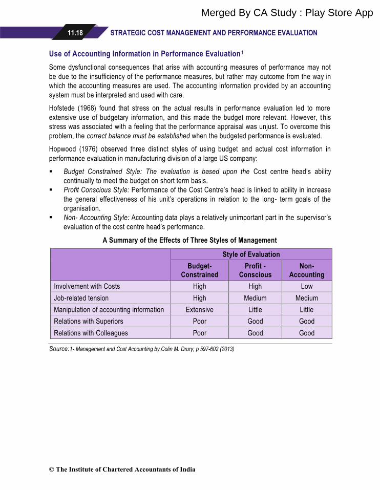
Hopwood (1976) observed three distinct styles of using budget and actual cost information in
performance evaluation in manufacturing division of a large US company:
▪ Budget Constrained Style: The evaluation is based upon the Cost centre head’s ability
continually to meet the budget on short term basis.
▪ Profit Conscious Style: Performance of the Cost Centre’s head is linked to ability in increase
the general effectiveness of his unit’s operations in relation to the long- term goals of the
organisation.
▪ Non- Accounting Style: Accounting data plays a relatively unimportant part in the supervisor’s
evaluation of the cost centre head’s performance.
A Summary of the Effects of Three Styles of Management
Style of Evaluation
Budget- Constrained
Profit - Conscious
Non-Accounting
Involvement with Costs High High Low
Job-related tension High Medium Medium
Manipulation of accounting information Extensive Little Little
Relations with Superiors Poor Good Good
Relations with Colleagues Poor Good Good
Source:1- Management and Cost Accounting by Colin M. Drury; p 597-602 (2013)
© The Institute of Chartered Accountants of India
Merged By CA Study : Play Store App
BUDGETARY CONTROL 11.19
BEYOND BUDGETING (BB)
To overcome these limitations a tool came into force known as Beyond Budgeting. Beyond
Budgeting is a leadership philosophy that relates to an alternative approach to budgeting which
should be used instead of traditional annual budgeting.
According to CIMA’s Official Terminology- ‘An idea that companies need to move
beyond budgeting because of the inherent flaws in budgeting especially when used to set contracts. It is argued that a range of techniques, such as rolling forecasts and market related targets, can take the place of traditional budgeting. ’
BB identifies its two main advantages.
▪ It is a more adaptive process than traditional budgeting.
▪ It is a decentralised process, unlike traditional budgeting where leaders plan and control organisations centrally.
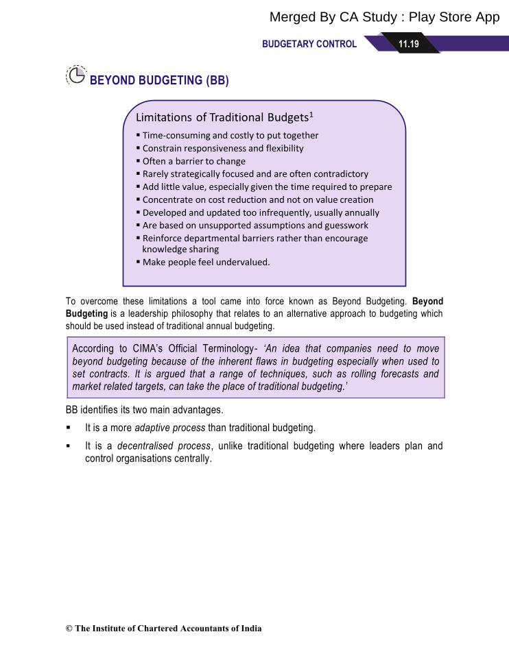
Limitations of Traditional Budgets1
▪ Time-consuming and costly to put together
▪ Constrain responsiveness and flexibility
▪ Often a barrier to change
▪ Rarely strategically focused and are often contradictory
▪ Add little value, especially given the time required to prepare
▪ Concentrate on cost reduction and not on value creation
▪ Developed and updated too infrequently, usually annually
▪ Are based on unsupported assumptions and guesswork
▪ Reinforce departmental barriers rather than encourage knowledge sharing
▪ Make people feel undervalued.
© The Institute of Chartered Accountants of India
Merged By CA Study : Play Store App
11.20 STRATEGIC COST MANAGEMENT AND PERFORMANCE EVALUATION
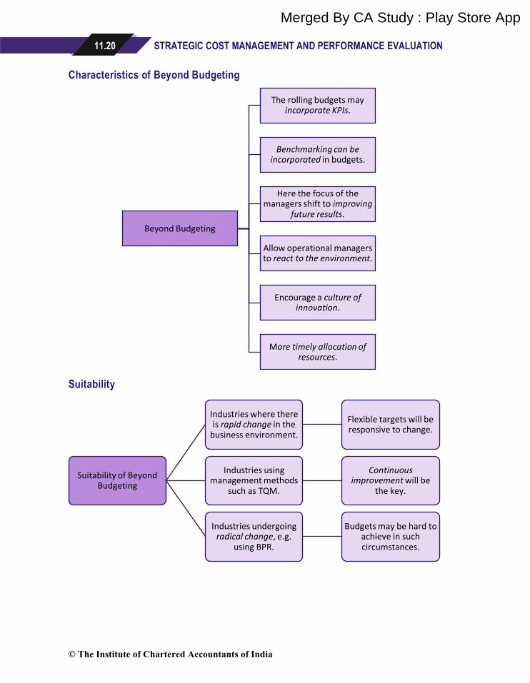
Characteristics of Beyond Budgeting
Suitability
Beyond Budgeting
The rolling budgets may incorporate KPIs.
Benchmarking can be incorporated in budgets.
Here the focus of the managers shift to improving
future results.
Allow operational managers to react to the environment.
Encourage a culture of innovation.
More timely allocation of resources.
Suitability of Beyond Budgeting
Industries where there is rapid change in the
business environment.
Flexible targets will be responsive to change.
Industries using management methods
such as TQM.
Continuous improvement will be
the key.
Industries undergoing radical change, e.g.
using BPR.
Budgets may be hard to achieve in such circumstances.
© The Institute of Chartered Accountants of India
Merged By CA Study : Play Store App
BUDGETARY CONTROL 11.21
Benefits of the 'Beyond Budgeting' Model
▪ Beyond budgeting helps managers to work in coordination to beat the competition. Internal
rivalry between managers is reduced as target shifts to competitors.
▪ Helps in motivating individuals by defining clear responsibilities and challenges.
▪ It eliminates some behavioural issues by making rewards team-based.
▪ Proper delegation of authority to operational managers who are close to the concerned action
and can react quickly.
▪ Operational managers do not restrict themselves to budget limits and focus on achieving key
ratios.
▪ It establishes customer-orientated teams.
▪ It creates information systems which provide fast and open information throughout the
organisation.
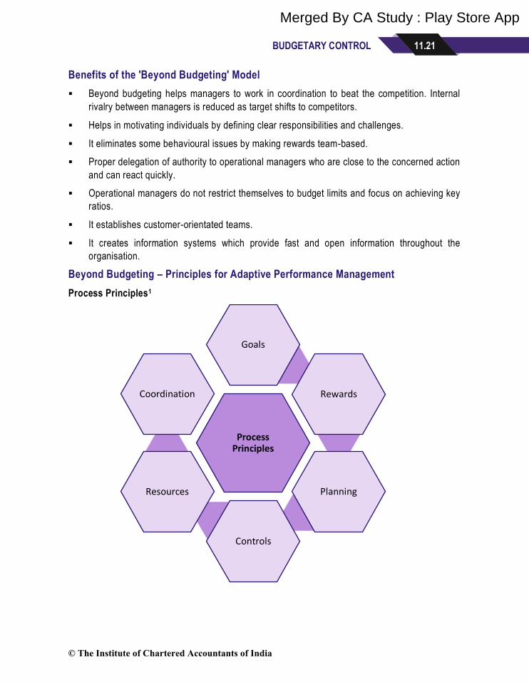
Beyond Budgeting – Principles for Adaptive Performance Management
Process Principles1
Process Principles
Goals
Rewards
Planning
Controls
Resources
Coordination
© The Institute of Chartered Accountants of India
Merged By CA Study : Play Store App

11.22 STRATEGIC COST MANAGEMENT AND PERFORMANCE EVALUATION
Goals Set aspirational goals aimed at continuous improvement, not fixed annual
targets.
Rewards Reward shared success based on relative performance, not on meeting
fixed
annual targets.
Planning Make planning a continuous and inclusive process, not an annual event.
Controls Base controls on relative key performance indicators (KPIs) and
performance trends, not variances against a plan.
Resources Make resources available as needed, not through annual budget
allocations.
Co-ordination Co-ordinate cross-company interactions dynamically, not through annual
planning cycles.
Leadership Principles1
Leadership Principles
Customer
Accountability
Performance
Freedom to Act
Governance
Information
© The Institute of Chartered Accountants of India
Merged By CA Study : Play Store App

BUDGETARY CONTROL 11.23
Customer Focus everyone on improving customer outcomes, not on meeting internal
targets.
Accountability Create a network of teams accountable for results, not centralised
hierarchies.
Performance Champion success as winning in the marketplace, not on meeting internal
targets.
Freedom to Act Give teams the freedom and capability to act, don’t merely require
adherence to plan.
Governance Base governance on clear values and boundaries, not detailed rules and
budgets.
Information Promote open and shared information, don’t restrict it to those who ‘need
to know’.
Implementation of Beyond Budgeting
There are nine steps that Hope and Fraser consider to be essential to implementing the Beyond
Budgeting approach.
Source: Beyond Budgeting: How Managers Can Break Free from the Annual Performance Trap by Jeremy Hope, Robin Fraser
Define the Case for Change and Provide
an Outline Vision
Be Prepared to Convince the Board
Get Started Design and
Implement New Processes
Train and Educate People
Rethink the Role of Finance
Change Behaviour –New Processes, Not Management Orders
Evaluate the Benefits
Consolidate the Gains
© The Institute of Chartered Accountants of India
Merged By CA Study : Play Store App

11.24 STRATEGIC COST MANAGEMENT AND PERFORMANCE EVALUATION
Traditional vs Beyond Budgeting Model
Source: Beyond Budgeting Info- Centre http://www.juergendaum.com/bb.htm
Outlined by Jeremy Hope
Traditional Budgeting
Management Model
Beyond Budgeting
Management Model
Targets and Rewards ▪ Incremental targets
▪ Fixed incentives
▪ Stretch goals
▪ Relative targets and
rewards
Planning and Controls ▪ Fixed annual plans
▪ Variance controls
▪ Continuous planning
▪ KPI’s & rolling forecasts
Resource and Coordination ▪ Pre-allocated resources
Central coordination
▪ Resources on demand
Dynamic Coordination
Organizational Culture ▪ Central control
▪ Focus on managing
numbers
▪ Local control of goals/
plans
▪ Focus on value creation
© The Institute of Chartered Accountants of India
Merged By CA Study : Play Store App

BUDGETARY CONTROL 11.25
Conclusion on Budgeting1
It has been proposed that budgeting is alive and well, though practice is evolving with new tools
and techniques. The conclusion are as follows:
▪ Budgeting is evolving, rather than becoming obsolete- it depends on trust and transparency.
▪ Shift from the top-down, centralised process to a more participative, bottom-up exercise in
many firms.
▪ It highlights the level of improvement that can be achieved even with relatively simple
modifications and a great deal of trust.
▪ Budgeting has changed, the change has been neither dramatic nor radical. Instead,
incremental improvements, with traditional budgets being supplemented by new tools and
techniques.
▪ Forecasting in fact is more important.
Source: 1-Better Budgeting A report on the Better Budgeting forum from CIMA and ICAEW July 2004- Driving Value Through
Strategic Planning and Budgeting, p7,9; Debating the traditional role of budgeting in organisations, p 5.
SUMMARY
▪ Budgetary Control is “Systematic control of an organization's operations through establishment
of standards and targets regarding income and expenditure, and a continuous monitoring and
adjustment of performance against them.”
▪ Characteristics those are common to businesses with effective budgetary cont rol include clarity
of marginal responsibility, challenging and achievable business targets, establishment of data
collection, analysis and reporting techniques, accountability of individual managers, shorter
time periods, timely variance reports, timely actions to prevent variances.
▪ Feedback and Feed-forward Control – Feedback Control refers to ‘Measurement of differences
between planned outputs and actual outputs achieved, and the modification of subsequent
action and/or plans to achieve future required results. Feedback control is an integral part of
budgetary control and standard costing systems.’
o A feedback system would simply compare the actual historical results with the budgeted
results.
o Feed-forward Control is defined as the ‘forecasting of differences between actual and
planned outcomes and the implementation of actions before the event, to avoid such
differences.’
▪ Behavioural aspects of Budgetary Controls – Many of the conflicts arise due to the human
nature of a budgetary control system. Managers do not always follow organisational goals,
they do not always think long term, they may be wary of moving away from the plan etc. This
© The Institute of Chartered Accountants of India
Merged By CA Study : Play Store App

11.26 STRATEGIC COST MANAGEMENT AND PERFORMANCE EVALUATION
provides a conflict between many of the goals of a budgetary control system which needs to be
considered at a strategic level when implementing such a system.
▪ Budget Slack – Budget affects the attitudes and behaviour of managers and used to motivate
the managers. Unrealistic demanding targets tend to affect manager’s performance adversely.
Allowing managers to set their own targets will introduce slack targets. This helps satisfy one
of the purposes of budgeting in that it can aid motivation. But it can have a detrimental impact
on the other purposes such as distorting the evaluation of actual performance if managers
incorporate 'slack' into the budget in order to make it easier to achieve.
▪ Budget level that motivates the best level of performance may not be achievable. In contrast,
the budget that is expected to be achieved motivates a lower level of performance as
managers no longer aspire to meet the budget target.
▪ Participation in Budget Setting Process – Budgets can be prepared centrally and subordinates
have little influence on the target setting. This called top down budget or imposed style
approach. The benefit of top down approach is that it can be produced quickly and involve less
management time than other options. However, there are significant risk of inaccurate budgets
being set that are also not acceptable to the subordinate managers. An alternative to top -down
approach is for the subordinate managers to participate in the preparation of their own budgets
and then these budgets to be reviewed by senior management. This is called bottom up
approach (sometimes referred participative approach). Participation must be used selectively;
but if it is used in the right circumstances, it has an enormous potential for encouraging the
commitment to organisational goals, improving attitudes towards budgeting system, and
increasing subsequent performance.
▪ Circumstances Where Top-Down Budget Setting is Preferable – Personality traits of the
participation limiting the benefits of participation, lack of managerial motivation at individual
level, highly programmable processes in the system, homogeneous units produced in stable
environment.
▪ Limitations of Traditional Budgets – time consuming, costly, constrain flexibility and
responsiveness, barrier to changes, contradictory, no focus on strategies, concentration on
cost reduction and not value creation, developed too frequently, based on guess work, raises
departmental barriers, discourage knowledge sharing, demotivate employees.
▪ Beyond Budgeting – An idea that companies need to move beyond budgeting because of the
inherent flaws in budgeting especially when used to set contracts. It is argued that a range of
techniques, such as rolling forecasts and market related targets, can take the place of
traditional budgeting.
▪ Characteristics of Beyond Budgeting – The rolling budgets may incorporate KPIs based on the
balanced scorecard which is linked to the organisation strategy, benchmarking with external
players may help better evaluation, focus on improving future results rather than dwelling on
past poor performances, allows operational managers to react to changing environment,
encourages culture for innovation, flexible and do not rely on obsolete figures.
© The Institute of Chartered Accountants of India
Merged By CA Study : Play Store App

BUDGETARY CONTROL 11.27
▪ Suitability for Beyond Budgeting – Rapidly changing business targets, organisation using TQM/
continuous improvement management techniques, organisations under business process
reengineering.
▪ Benefits of Beyond Budgeting model – Internal rivalry among managers is reduced as focus
shifts on competitors, motivating employees, proper delegation of authority of operational
managers, customer-oriented teams, fast and open information across organisation.
▪ Steps essential for implementing Beyond Budgeting– Define the Case for Change and Provide
an Outline Vision; Be Prepared to Convince the Board; Get Started; Design and Implement
New Processes; Train and Educate People; Rethink the Role of Finance; Change Behaviour –
New Processes, Not Management Orders; Evaluate the Benefits and Consolidate the Gains.
TEST YOUR KNOWLEDGE
Feedforward Control and Feedback Control
1. EW Partners, a leading strategy and management consulting firm is preparing its budgets for
the year to 31 March 2020. One of partner ‘W’ is concerned about liquidity, he argued, that a
firm with adequate liquidity has less risk of being unable to meet their liabilities than an illiquid
one. Where a firm has adequate liquidity, there is also the possibility of enriched profitability
through reduced interest outlay or increased interest income, together with greater financial
flexibility to negotiate enhanced terms with suppliers and financiers or participate in new
business opportunities. Accordingly, he desires to reduce the firm’s CC to zero by 30
September 2019 and to have a positive cash balance of `145,000 by the end of the year.
Required
COMPARE and CONTRAST, feedforward control and feedback control in context of the
above information.
Participative Budget
2. SPM, a leading school of management in the heart of India’s financial centre of Mumbai,
preparing its budget for 2019. In previous years, the director of the school has prepared the
budget without the participation of senior staff and presented it to the school board for
approval.
Last year the SPM board blasted the director over the lack of participation of his senior staff
in the budget process for 2018 and requested that for the 2019 budget the senior staff were
to be involved.
Required
LIST the potential advantages and disadvantages to the SPM of involving the senior staff in
the budget preparation process.
© The Institute of Chartered Accountants of India
Merged By CA Study : Play Store App

11.28 STRATEGIC COST MANAGEMENT AND PERFORMANCE EVALUATION
Behavioural Aspects of Budgetary Control
3. History of the Company
Great Bus Tours Co. Ltd. (GBTCL) is an open top double-decker bus sightseeing company,
particularly identified with its special red and cream-colored buses. It commenced operating in
small town of Meghalaya in June 2014 with four buses and as of 2018 operated over 44 buses in
north east region of India. GBTCL operates five routes with stops at tourist destinations. The
company runs hop-on, hop-off bus tours of various hills, with one 24-hour ticket valid for unlimited
journeys on the route.
Budget Process/ Incentive Plan
As a part of management performance control and incentive scheme it has been following
participative budgeting approach. In GBTCL, budgeting is a joint process in which functional
divisions develop their plans in conformity with corporate goals for the next financial year.
Based on these plans, divisions prepare functional budgets and send to the appropriate
management for review and approval. The budgets after the incorporation of the feedback
and suggestions received from the said management, are finalised for the implementation.
Then, finalised budgets are used as yardstick for performance measurement. Comparing the
actual performance with the yardstick, bonus and other performance related incentives are
considered. The higher management believe that this performance control and incentive
scheme is very helpful to measure the performance and fixing responsibilities for the
responsibility centres.
Budgeted Income Statement (`’000)
Revenue 1,13,800
Less:
Variable Costs-
Direct Material (Fuel, Lubricants and Sundries) 13,600
Direct Labour 40,500
Variable Overheads 7,700
Fixed Costs-
Operating Overheads (Buses, Garage, Salaries) 18,100
Marketing and Administration 10,700
Profit/ (Loss) before taxes 23,200
Tabel-1
Current Year’s Income Statement (`’000)
Revenue 93,500
Less:
Variable Costs:
Direct Material (Fuel, Lubricants, and Sundries) 19,600
Direct Labour 37,700
© The Institute of Chartered Accountants of India
Merged By CA Study : Play Store App

BUDGETARY CONTROL 11.29
Variable Overheads 6,200
Fixed Costs:
Operating Overheads (Buses, Garage, Salaries) 20,150
Marketing and Administration 10,100
Profit/ (Loss) before taxes (250)
Tabel-2
Other Information
Surprisingly above given current year’s actual results were not up to the mark. Actual results
were clearly showing adverse performance in comparison with budgeted figures.
Managers of GBTCL were upset because they did not receive the bonus. Ms. Maggie, Tour
Manager of Route No. 3, said –
“We lost 2 month’s revenue and fuel prices are almost doubled. We did our best but these
circumstances were beyond our control and we should not penalize at all.”
In support of her statement, Ms. Meggie provided following additional information –
(a) Rain is common in Northern Region. But, the past year set a record in numbers. In July,
the expected average was 1,577 mm and received was 1,810 mm, In August the
expected average rain was 990 mm and actual received was 1,535 mm. Heavy rain in
these two months disrupted normal life of the region.
(b) The fuel prices have risen almost continuously since last year due to surge in global
crude prices.
(c) Additional operational expenses `22,00,000 also incurred to remove the milky
appearance and give the stainless a nice new look effected by heavy rain.
She claimed that –
“Revised budget with consideration of the above factors would give different results and lead
to different conclusions”
Required
ANALYSE the tour manager’s view.
Beyond Budgeting
4. The Board of Directors meeting of Kyoto Motors Ltd., a car manufacturing company is to be
scheduled to be held in another ten days. One of the items, as per agenda, to be discussed in
the meeting is the present budgeting system of the company. Your organisation is at present,
using budgets for control which are prepared mostly on traditional basis. The CEO of your
company wants to propose to the Board to use Beyond Budgeting instead of traditional
budgeting in the company on experimental basis. Therefore, you, the Management
Accountant has been asked by your CEO to explore the possibilities of introducing Beyond
Budgeting (BB) system in the company.
© The Institute of Chartered Accountants of India
Merged By CA Study : Play Store App

11.30 STRATEGIC COST MANAGEMENT AND PERFORMANCE EVALUATION
Required
Specifically, you are required to PREPARE notes to your CEO to be used for his presentation
at the meeting on:
(i) the major limitations of traditional budgets.
(ii) the advantages available in Beyond Budgeting.
(iii) the nature of Beyond Budgeting.
(iv) the benefits that can be enjoyed from Beyond Budgeting.
(v) the suitability of Beyond Budgeting to the company.
ANSWERS/ SOLUTIONS
1. In feed-forward control instead of actual results being compared against desired results,
forecasts are made of what results are expected to be at some future time . If these
expectations differ from what is desired, control actions are taken that will minimize these
gaps.
In the scenario, EW Partners has following 2 expectations–
- the first of these is to reduce the CC to zero by 30 Sep 2019 and
- the second is to have a positive cash balance of `145,000 by 31 March 2020.
Therefore, to achieve above expectations, a cash budget will be prepared based on various
functional budgets showing cash inflows and outflows for each month so that the firm can
identify its anticipated monthly cash balance. This can then be compared with the firm’s
expectations to see if their cash balance objectives are being achieved. However, if the
objectives are not met by these budgets, these budgets may need to be revised by changing
the levels of activities. It is the process of feedforward control.
Feedback control involves monitoring results achieved against desired results and taking
whatever corrective action is necessary if a deviation exists.
Thus, in the case of EW Partners, a comparison of the actual monthly cash balance can be
made against the budgeted cash balance for that month. As with any budget and actual
comparison there may be an adverse or favorable variance. If this is substantial, then further
analysis may be needed to determine its reason. It may be that costs above budgets, cash
receipts lower than expected or receivables took less time to pay than expected, or payables
were paid later than expected. This comparison process is feedback control.
Conclusion
Feedforward control attempts to take corrective action before an event, whereas feedback
control takes corrective action after the event.
© The Institute of Chartered Accountants of India
Merged By CA Study : Play Store App

BUDGETARY CONTROL 11.31
2. There are potential advantages and disadvantages of the involvement of staff in the
preparation of the budget.
Potential advantages include:
▪ Senior staff may agree to accept the targets because they would take ownership of it as their budget.
▪ Senior staff may have a better understanding of what results can be achieved and at what costs. For example, they may have a better knowledge of individual courses and how they may be delivered more efficiently and cost effectively.
▪ Senior staff cannot blame unrealistic goals as an excuse for not achieving budget expectations.
▪ Senior staff would feel that they are being appreciated for the value that their experience brings to the running of the management school.
▪ Senior staff may get the opportunity to discuss organisational issues, in which an exchange of information and ideas can help to solve problems and agree future act ions.
Potential disadvantages include:
▪ Senior staff may be excellent academically but could lack the practical knowledge required to formulate their budget.
▪ Senior staff may limit the benefits of participation due to personality traits of participants.
▪ Senior staff may consume a great deal of time arguing with each other (and with the school director).
Senior staff may decide among themselves to artificially inflate the proposed budget so that it is easier for them to attain the cost targets they have set.
3. Analysis of Issue
It appears that GBTCL has been badly hit by the weather – high rain in July and August have
led to a slump in business. Revenue have seen a fall of 18% over the budgeted figure. Direct
Material (most of the fuel) is 21% of the Sales (compared to 12% of budgeted level) because
of hike in fuel price. Variable Overheads are almost same. However, interestingly, there is a saving of `1,50,000 in Operating Overheads as compared to the budgeted figure after
catering additional Operational Expenses of `22,00,000 (for removal of milky appearance
etc.). Furthermore, there is reduction in Marketing & Administration Cost. The ratio of Salary
to Sales rose to 40% in 2018 from 36% (as budgeted). This appears to be atypical. Instead,
there should be a cut in this ratio due to slump in business.
Award of bonus in case of losses is not justified and managers should be held accountable
for their operations. However, they should not be held accountable for the events beyond
their control. A manager cannot control movements in fuel price, yet he/ she is supposed to
have the most information and he/ she is expected to correctly forecast movements in the
prices of fuel. Managers shouldn't be penalized for the uncontrollable events.
© The Institute of Chartered Accountants of India
Merged By CA Study : Play Store App

11.32 STRATEGIC COST MANAGEMENT AND PERFORMANCE EVALUATION
Accordingly, in GBTCL, there should be revision in the budget to account uncontrollable
events. Refer Table-3.
Revised Budgeted Income Statement (`’000)
Revenue* 94,833
Less:
Variable Costs-
Direct Material** (Fuel, Lubricants, and Sundries) 19,879
Direct Labour 33,750
Variable Overheads 6,417
Fixed Costs-
Operating Overheads (Buses, Garage, Salaries) 20,300
Marketing and Administration 10,700
Profit/ (Loss) before taxes 3,787
Tabel-3
*10 months revenue; ** at actual price levels
The Revised Profit Margin has come down to 4% as against the Target Profit Margin of 20%.
This clearly indicates that the performance was benchmarked against the higher target. If
original budget figure is used to measure the performance, it will punish employees for the
reason which are beyond their control.
GBTCL is not too far away from Revised Profit Margin. Therefore, at least some bonus may
be considered to be awarded to the employees which may create more employee loyalty and
may be beneficial for long term.
Further, continuous monitoring of Budget Performance (achievement/ failure) in GBTCL is
essential to overcome this situation. This helps to identify where revisions are required in the
budget to account changing conditions, errors, modification to company’s plan etc. Monitoring
of Budget Performance should be the responsibility of the managers in GBTCL. The essence
of the effective monitoring of Budget Performance is that the managers should provide
accurate, relevant, actionable information on time to the appropriate management level so
that budget can give a realistic target to measure the performance.
It is also important to note that at the time of revising the budget, the primary budget as well
as past information should not be ignored as they are the basis for preparing all budgets.
4. (i) Limitations of Traditional Budgets
▪ Time-consuming and costly to put together.
▪ Constrain responsiveness and flexibility.
▪ Often a barrier to change.
© The Institute of Chartered Accountants of India
Merged By CA Study : Play Store App

BUDGETARY CONTROL 11.33
▪ Rarely strategically focused and are often contradictory.
▪ Add little value, especially given the time required to prepare.
▪ Concentrate on cost reduction and not on value creation.
▪ Developed and updated too infrequently, usually annually.
▪ Are based on unsupported assumptions and guesswork.
▪ Reinforce departmental barriers rather than encourage knowledge sharing.
▪ Make people feel undervalued.
(ii) Advantages of Beyond Budgeting (BB)
BB identifies its two main advantages.
▪ It is a more adaptive process than traditional budgeting.
▪ It is a decentralised process, unlike traditional budgeting where leaders plan and
control organisations centrally.
(iii) Nature of 'Beyond Budgeting'
▪ Budgeting is evolving, rather than becoming obsolete- it depends on trust and
transparency.
▪ Shift from the top-down, centralised process to a more participative, bottom-up
exercise in many firms.
▪ It highlights the level of improvement that can be achieved even with relatively
simple modifications and a great deal of trust.
▪ Budgeting has changed, the change has been neither dramatic nor radical. Instead,
incremental improvements, with traditional budgets being supplemented by new
tools and techniques.
▪ Forecasting in fact is more important.
(iv) Benefits of the 'Beyond Budgeting' Model
▪ Beyond budgeting helps managers to work in coordination to beat the competition.
Internal rivalry between managers is reduced as target shifts to competi tors.
▪ Helps in motivating individuals by defining clear responsibilities and challenges.
▪ It eliminates some behavioural issues by making rewards team-based.
▪ Proper delegation of authority to operational managers who are close to the
concerned action and can react quickly.
▪ Operational managers do not restrict themselves to budget limits and focus on
achieving key ratios.
© The Institute of Chartered Accountants of India
Merged By CA Study : Play Store App
11.34 STRATEGIC COST MANAGEMENT AND PERFORMANCE EVALUATION
▪ It establishes customer-orientated teams.
▪ It creates information systems which provide fast and open information throughout
the organization
(v) Suitability of Beyond Budgeting to the Company
Since Kyoto Motors Ltd. is a car manufacturing company and presently adopting
Traditional Costing system. Moreover, Automobile industry goes through rapid changes
in its business environment. So, the company can definitely use Beyond Budgeting to
improve the control system and beat the competition. Beyond Budgeting lies an agile,
holistic approach based on self-organisation. This will also help the managers to work in
close coordination with each other with motivation which in turn will beat the competition.
© The Institute of Chartered Accountants of India
Merged By CA Study : Play Store App
12
STANDARD COSTING
LEARNING OUTCOMES
After studying this chapter, you will be able to:
❑ Calculate advanced variances
❑ Interpret Variances
❑ Identify and Explain the relationship of the Variances
❑ Apply Standard Costing Methods including the Reconciliation of Budgeted and Actual Profit Margins
❑ Explain the wider issues involved in changing mix e.g. Cost, Quality, and Performance Measurement issues
❑ Analyse and Evaluate Past Performance using the results of variance analysis
❑ Use Variance Analysis to assess how Future Performance of an organisation can be improved
© The Institute of Chartered Accountants of India
Merged By CA Study : Play Store App

12.2 STRATEGIC COST MANAGEMENT AND PERFORMANCE EVALUATION
CHAPTER OVERVIEW
ANALYSIS OF ADVANCED VARIANCES
Variance analysis is examinable both at Intermediate Level (Cost and Management Accounting)
and at Final Level (Strategic Cost Management and Performance Evaluation). One main difference
in syllabus between the two papers is that the Final Level syllabus includes analysis of
advanced variances, as follows:
▪ Planning and Operational Variances
▪ Variance Analysis in Activity Based Costing
▪ Learning Curve Impact on Variances
▪ Relevant Cost Approach to Variance Analysis
▪ Variance Analysis and Throughput Accounting
▪ Variance Analysis in Advanced Manufacturing Environment
▪ Variance Analysis in Service Industry
▪ Variance Analysis in Public Services
Planning & Operational Variances
When the current environmental conditions are different from the anticipated environmental
conditions (prevailing at the time of setting standard or plans) the use of routine analysis of
variance for measuring managerial performance is not desirable / suitable. The variance analysis
can be useful for measuring managerial performance if the variances computed are determined on
the basis of revised targets / standards based on current actual environmental conditions.
© The Institute of Chartered Accountants of India
Merged By CA Study : Play Store App

STANDARD COSTING 12.3
In order to deal with the above situation i.e. to measure managerial performance with reference to
material, labour and sales variances, it is necessary to compute the Planning and Operational
Variances.
A Planning Variance simply compares a revised standard to the original standard.
An Operational Variance simply compares the actual results against the revised amount.
Operating Variances would be calculated after the planning variances have been established and
are thus a realistic way of assessing performance.
Planning Variance
Classification of variances caused by ex-ante budget allowances being changed to an ex post
basis. Also, known as a revision variance.
Operational Variance
Classification of variances in which non-standard performance is defined as being that which
differs from an ex post standard. Operational variances can relate to any element of the standard
product specification.
Standard ex ante
Before the event. An ex ante budget or standard is set before a period of activity commences.
Standard, ex post
After the event. An ex post budget, or standard, is set after the end of a period of activity, when it
can represent the optimum achievable level of performance in the conditions which were
experienced. Thus, the budget can be flexed, and standards can reflect factors such as
unanticipated changes in technology and in price levels. This approach may be used in
conjunction with sophisticated cost and revenue modelling to determine how far both the plan and
the achieved results differed from the performance that would have been expected in the
circumstances which were experienced.
© The Institute of Chartered Accountants of India
Merged By CA Study : Play Store App

12.4 STRATEGIC COST MANAGEMENT AND PERFORMANCE EVALUATION
Example
Factor Original Standards
(ex-ante)
Revised Standards
(ex-post)
Actual
(4,500 units)
X 4,500 units×2
Kgs×`12.50
`1,12,500 4,500 units×2.25
Kgs×`11.50
`1,16,437.50 8,750
Kgs×`13
`1,13,750
Traditional Variances
Usage Variance = (9,000 Kgs. – 8,750 Kgs.) × `12.50
= `3,125 (F)
Price Variance = (`12.50 – `13.00) × 8,750 Kgs.
= `4,375 (A)
Total Variance = `3,125 (F) + `4,375 (A)
= `1,250 (A)
Operational Variances
Usage Variance = (10,125 Kgs. – 8,750 Kgs.) × `11.50
= `15,812.50 (F)
Price Variance = (`11.50 – `13) × 8,750 Kgs.
= `13,125 (A)
Total Variance = `15,812.50 (F) + `13,125 (A)
= `2,687.50 (F)
Planning Variances
Usage Variance = (9,000 Kgs. – 10,125 Kgs.) × `12.50
= `14,062.50 (A)
Price Variance = (`12.50 – `11.50) × 10,125 Kgs.
= `10,125 (F)
Total Variance = `14,062.50 (A) + `10,125 (F)
= `3,937.50 (A)
© The Institute of Chartered Accountants of India
Merged By CA Study : Play Store App

STANDARD COSTING 12.5
Direct Material Usage Variance
Traditional Variance
Actual vs. Original Standard
[Standard Quantity – Actual Quantity] ×
Standard Price
Direct Material Price Variance
Traditional Variance
Actual vs. Original Standard
[Standard Price – Actual Price] × Actual
Quantity
Note
Direct Material Usage Operational Variance using Standard Price, and the Direct Material Price Planning Variance based on Actual Quantity can also be calculated. This approach reconciles the Direct Material Price Variance and Direct Material Usage Variance calculated in part.
Planning Variance
Revised Standard vs. Original Standard
[Standard Quantity – Revised Standard Quantity]
× Standard Price
Operational Variance
Actual vs. Revised Standard
[Revised Standard Quantity – Actual Quantity] ×
Revised Standard Price
Planning Variance
Revised Standard vs. Original Standard
[Standard Price – Revised Standard Price] ×
Revised Standard Quantity
Operational Variance
Actual vs. Revised Standard
[Revised Standard Price – Actual Price] × Actual
Quantity
© The Institute of Chartered Accountants of India
Merged By CA Study : Play Store App

12.6 STRATEGIC COST MANAGEMENT AND PERFORMANCE EVALUATION
Like Material Variances, here also Labour Efficiency and Wage Rate Variances should also be
adjusted to reflect changes in environmental conditions that prevailed during the period.
Illustration
HDR Ltd produces units and incurs labour costs. A change in technology after the preparation of
the budget resulted in a 25% increase in standard labour efficiency, such that it is now possible to
produce 10 units instead of 8 units using 8 hours of labour- giving a revised standard labour
requirement of 0.80 hours per unit. Details of actuals and budgeted for period XII are:
Grade Original Standards
(ex-ante)
Revised Standards
(ex-post)
Actual
(1,100 units)
X 1,100 units ×
1 hrs. × ` 10
` 11,000 1,100 units ×
0.80 hrs. × ` 10.00
` 8,800 1,200 hrs. ×
` 8.50
` 10,200
Required
(i) CALCULATE the variances for ‘X’ by
(a) Traditional Variance Analysis; and
(b) An approach which distinguishes between Planning and Operational Variances.
(ii) COMMENT on the results.
Solution
(i) (a) Traditional Variances
Efficiency Variance = (1,100 hrs. – 1,200 hrs.) × `10
= `1,000 (A)
Rate Variance = (`10 – `8.50) × 1,200 hrs.
= `1,800 (F)
Total Variance = `1,000 (A) + `1,800 (F) = `800 (F)
(b) Operational Variances
Efficiency Variance = (880 hrs. – 1,200 hrs.) × `10.00
= `3,200 (A)
Rate Variance = (`10.00 – `8.50) × 1,200 hrs.
= `1,800 (F)
Total Variance = `3,200 (A) + `1,800 (F) = `1,400 (A)
Planning Variances
Efficiency Variance = (1,100 hrs. – 880 hrs.) × `10
= `2,200 (F)
Rate Variance = (`10 – `10) × 800 hrs.
= `0
Total Variance = `2,200 (F) + `0 = `2,200 (F)
© The Institute of Chartered Accountants of India
Merged By CA Study : Play Store App

STANDARD COSTING 12.7
(ii) Comment
In this case, the separation of the labour cost variance into operational and planning
components shows a large problem in the area of labour efficiency than might otherwise have
been indicated. The operational variances are based on the revised (ex post) standard and
this gives a more meaningful performance benchmark than the original (ex-ante) standard.
Direct Labour Efficiency Variance
Traditional Variance Actual vs. Original Standard
[Standard Time – Actual Time] × Standard Rate
Direct Labour Rate Variance
Traditional Variance Actual vs. Original Standard
[Standard Rate – Actual Rate] × Actual Time
Note
Direct Labour Efficiency Operational Variance using Standard Rate, and the Direct Labour Rate Planning Variance based on Actual Hours can also be calculated. This approach reconciles the Direct Labour Rate Variance and Direct Labour Efficiency Variance calculated in part.
Planning Variance Revised Standard vs. Original Standard
[Standard Time – Revised Standard Time] × Standard Rate
Operational Variance Actual vs. Revised Standard
[Revised Standard Time – Actual Time] × Revised Standard Rate
Planning Variance Revised Standard vs. Original Standard
[Standard Rate – Revised Standard Rate] × Revised Standard Time
Operational Variance Actual vs. Revised Standard
[Revised Standard Rate – Actual Rate] × Actual Time
© The Institute of Chartered Accountants of India
Merged By CA Study : Play Store App

12.8 STRATEGIC COST MANAGEMENT AND PERFORMANCE EVALUATION
The conventional Sales Volume Variance reports the difference between actual and budgeted
sales valued at the standard price per unit. The variance just indicates whether sales volume is
greater or less than expected. It does not indicate how will sales management has performed. In
order to assess the performance of sales management, market conditions prevailing during the
period should be taken into consideration.
Accordingly, the sales volume variance can be sub-divided into a planning variance (market size
variance) and operational variance (market share variance).
A Planning Variance simply compares a revised standard to the original standard. An
Operational Variance simply compares the actual results against the revised amount.
Controllable Variances are those variances which arises due to inefficiency of a cost centre
/department. Uncontrollable Variances are those variances which arises due to factors beyond
the control of the management or concerned department of the organization.
Variance Analysis in Activity Based Costing
Variance analysis can be applied to activity costs (such as setup costs , product testing, quality
testing etc.) to gain understanding into why actual activity costs vary from activity costs in the
static budget or in the flexible budget. Interpreting cost variances for different activ ities requires
understanding whether the costs are output unit-level, batch level, product sustaining, or facility
sustaining costs1.
We use the similar track to variance analysis for activity-based costing as for traditional costing.
The price variance is the difference between standard price and actual price for the actual quantity
of input used for each cost driver. The efficiency variance measures the difference between the
actual amount of cost driver units used, and the standard allowed to make the output. We multiply
the difference in quantities by the standard price per cost driver to get the rupee value of the
variance2.
ABC approach is based on the assumption that the overheads are basically variable (but variable
with the delivery numbers and not the units output). The efficiency variance reports the cost impact
of undertaking more or less activities than standard, and the expenditure variance reports cost
impact of paying more or less than standard for the actual activities undertaken 3.
Source: 1- Cost Accounting: A Managerial Emphasis, 13/e by Charles T. Horngren, p275; Managerial Accounting: 2- An
Introduction to Concepts, Methods and Uses by Michael W. Maher, Clyde P. Stickney, Roman L. Weil, p 362; 3-
Performance Operations by Robert Scarlett, p119.
Illustration
N & S Co. (NSC) is a multiple product manufacturer. NSC produces the unit and all overheads are
associated with the delivery of units to its customers.
© The Institute of Chartered Accountants of India
Merged By CA Study : Play Store App
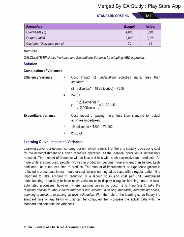
STANDARD COSTING 12.9
Particulars Budget Actual
Overheads (`) 4,000 3,900
Output (units) 2,000 2,100
Customer Deliveries (no.’s) 20 19
Required
CALCULATE Efficiency Variance and Expenditure Variance by adopting ABC approach.
Solution
Computation of Variances
Efficiency Variance = Cost Impact of undertaking activities more/ less than
standard
= (21 deliveries* – 19 deliveries) × `200
= `400 F
(*) 20 Deliveries
2,100 units2,000 units.
Expenditure Variance = Cost impact of paying more/ less than standard for actual
activities undertaken
= 19 deliveries × `200 – `3,900
= `100 (A)
Learning Curve- Impact on Variances
Learning curve is a geometrical progression, which reveals that there is steadily decreasing cost
for the accomplishment of a given repetitive operation, as the identical operation is increasingly
repeated. The amount of decrease will be less and less with each successive unit produced. As
more units are produced, people involved in production become more efficient than before. Each
additional unit takes less time to produce. The amount of improvement or experience gained is
reflected in a decrease in man-hours or cost. Where learning takes place with a regular pattern it is
important to take account of reduction in a labour hours and cost per unit`. Automated
manufacturing is unlikely to have much variation or to display a regular learning curve. In less -
automated processes, however, where learning curves do occur , it is important to take the
resulting decline in labour hours and costs into account in setting standards, determining prices,
planning production, or setting up work schedules. With the help of the learning curve theory the
standard time of any batch or unit can be computed then compare the actual data with the
standard and compute the variances.
© The Institute of Chartered Accountants of India
Merged By CA Study : Play Store App

12.10 STRATEGIC COST MANAGEMENT AND PERFORMANCE EVALUATION
Illustration
City International Co. is a multiproduct firm and operates standard costing and budgetary control
system. During the month of June firm launched a new product. An extract from performance
report prepared by Sr. Accountant is as follows:
Particulars Budget Actual
Output 30 units 25 units
Direct Labour Hours 180.74 hrs. 118.08 hrs.
Direct Labour Cost `1,19,288 ` 79,704
Sr. Accountant prepared performance report for new product on certain assumptions but later on
he realized that this new product has similarities with other existing product of the company.
Accordingly, the rate of learning should be 80% and that the learning would cease after 15 units.
Other budget assumptions for the new product remain valid.
The original budget figures are based on the assumption that the labour has learning rate of 90%
and learning will cease after 20 units, and thereafter the time per unit will be the same as the time
of the final unit during the learning period, i.e. the 20th unit. The time taken for 1 st unit is 10 hours.
Required
Show the variances that reconcile the actual labour figures with revised budgeted figures (for
actual output) in as much detail as possible.
Note:
The learning index values for a 90% and a 80% learning curve are −0.152 and −0.322
respectively.
[log 2 = 0.3010, log 3 = 0.47712, log 5 = 0.69897, log 7 = 0.8451, antilog of 0.6213 = 4.181, antilog
of 0.63096 = 4.275]
Solution
Working Note
The usual learning curve model is
y = axb
Where
y = Average time per unit for x units
a = Time required for first unit
x = Cumulative number of units produced
b = Learning coefficient
© The Institute of Chartered Accountants of India
Merged By CA Study : Play Store App

STANDARD COSTING 12.11
W.N.1
Time required for first 15 units based on revised learning curve of 80% (when the time
required for the first unit is 10 hours)
y = 10 × (15) –0.322
log y = log 10 − 0.322 × log 15
log y = log 10 − 0.322 × log (5 × 3)
log y = log 10 − 0.322 × [log 5 + log 3]
log y = 1 − 0.322 × [0.69897 + 0.47712]
log y = 0.6213
y = antilog of 0.6213
y = 4.181 hours
Total time for 15 units = 15 units × 4.181 hours
= 62.72 hours
Time required for first 14 units based on revised learning curve of 80% (when the time
required for the first unit is 10 hours)
y = 10 × (14) –0.322
log y = log10 − 0.322 × log 14
log y = log10 − 0.322 × log (2 × 7)
log y = log10 − 0.322 × [log 2 + log 7]
log y = 1 − 0.322 × [0.3010 + 0.8451]
log y = 0.63096
y = antilog of 0.63096
y = 4.275 hrs
Total time for 14 units = 14 units × 4.275 hrs
= 59.85 hrs
Time required for 25 units based on revised learning curve of 80% (when the time required for
the first unit is 10 hours)
Total time for first 15 units = 62.72 hrs
Total time for next 10 units = 28.70 hrs [(62.72 − 59.85) hours × 10 units]
Total time for 25 units = 62.72 hrs + 28.70 hrs
= 91.42 hrs
© The Institute of Chartered Accountants of India
Merged By CA Study : Play Store App

12.12 STRATEGIC COST MANAGEMENT AND PERFORMANCE EVALUATION
W.N.2
Computation of Standard and Actual Rate
Standard Rate = 1,19,288
180.74 hrs.
`
= `660.00 per hr.
Actual Rate = 79,704
118.08 hrs.
`
= `675.00 per hr.
W.N.3
Computation of Variances
Labour Rate Variance = Actual Hrs × (Std. Rate – Actual Rate)
= 118.08 hrs × (`660.00 – `675.00)
= `1,771.20 (A)
Labour Efficiency Variance = Std. Rate × (Std. Hrs – Actual Hrs)
= `660 × (91.42 hrs – 118.08 hrs)
= `17,595.60 (A)
Statement of Reconciliation (Actual Figures Vs Budgeted Figures)
Particulars `
Actual Cost 79,704.00
Less: Labour Rate Variance (Adverse) 1,771.20
Less: Labour Efficiency Variance (Adverse) 17,595.60
Budgeted Labour Cost (Revised)* 60,337.20
Budgeted Labour Cost (Revised)*
= Std. Hrs. × Std. Rate
= 91.42 hrs. × `660
= `60,337.20
Relevant Cost Approach to Variance Analysis
Traditional approach to variance analysis is to compute variances based on total actual cost for
production inputs and total standard cost applied to the production output. This is ambiguous,
when inputs are limited. Failure to use limited inputs properly leads not only to increased
acquisition cost but also to a lost contribution. Therefore, it is necessary to consider the lost
contribution in variance analysis. When this approach is used, price or expenditure variances are
not affected.
© The Institute of Chartered Accountants of India
Merged By CA Study : Play Store App

STANDARD COSTING 12.13
Variance Analysis and Throughput Accounting
Variance analysis has no emphasis on the constrained resources. Instead, it is based on the
efficiency and cost of operation of each part of the manufacturing system, rather than the ability of
the entire system to generate a profit. Thus, a firm may find that it attains excellent efficiency and
price variances by having long manufacturing rounds and buying in large quantities. A system
based on constraint management will likely show very odd results under a variance reporting
system. For example, when a terminal upstream from the constrained resource runs out of work, a
manager functioning under throughput accounting system will shut it down in order to avoid the
formation of an unnecessary level of work-in-process inventory. However, this will result into a
negative labor efficiency variance, since the terminal’s staff is not actively producing anything.
Throughput accounting does use variance analysis, but not the ones used by a traditional system.
Instead, its main emphasis is on tracking variations in the size of the inventory buffer placed
before the constrained resource, to confirm that the constraint is never halted due to an inventory
shortage. Variance Analysis in Advanced Manufacturing Environment/ High-Technology Firms
The variance analysis generally applies to all types of organizations; however, high-technology
firms like Audio Technology, Automotive, Computer Engineering, Electrical and Electronic
Engineering, Information Technology, Medical devices, Nanotechnology, Semiconductors,
Telecommunication apply the model somewhat differently. Now much of electronic industry is
highly automated. A large part of manufacturing process is computerized. In the high-technology
environment that is emerging, many costs that once were largely variable have become fixed, most
becoming committed fixed cost. Some high technology manufacturing organizations have found
that the two largest variable costs involve materials and power to operate machines. In these
companies, the emphasis of variance analysis is placed on direct materials and variable
manufacturing overhead.
Much of the manufacturing labour consists of highly skilled experts/ operators/ programmers are
largely committed cost. Firms don’t want to take risk losing such highly trained personnel even
during an economic downturn. The result is less direct labour and more overhead. For these firms
labour variances may no longer be meaningful because direct labour is a committed cost, not a
cost expected to vary with output.
Standard Costing in Service Sector
Standard Costing can be equally applicable for various types of industries for example
accountants, solicitors, dentists, hairdressers, transport companies and hotels. Service industries
comprise a wide range of different businesses that differ in size and types of service provided.
Standard costing and variance analysis is more tough to apply to service sector organizations as
major portion of their cost is comprised of overhead expenses rather than production expenses.
While traditional variance analysis of overheads does not deliver very useful information for
overheads control purposes, application of activity based costing can provide an effective basis for
variance analysis of overheads in service sector organizations although this may need significant
time and effort in the implementation of a MIS.
© The Institute of Chartered Accountants of India
Merged By CA Study : Play Store App

12.14 STRATEGIC COST MANAGEMENT AND PERFORMANCE EVALUATION
McDonaldization
McDonaldization is a process of rationalisation, which takes a task and breaks it down into smaller tasks. This is repeated until all tasks have been broken down to the smallest possible level. The resulting tasks are then rationalised to find the single most efficient method for completing each task. All other methods are then deemed inefficient and discarded1.
The impact of McDonaldization is that standards can be more accurately set and assessed. It can be easily ascertained that how much time and cost should go into each activity. The principles can be applied to many other services, such as hairdressing, dentistry, or opticians' services.
Source: www.mcdonaldization.com/whatisit.shtml
Standard Costing in Public Sector
In order to cost control in public sector (e.g. street cleaning refuse disposal and so on), regular
variance analysis is required. Actual unit costs should be calculated on a monthly basis and
compared with estimated unit cost. To achieve this comparison, information needs to be
maintained about the unit of service adopted. For example, statistics would be maintained on the
number of visits made and the number of hours worked. In this example, time recording may be
beneficial in providing the detailed information necessary for var iance analysis. Actual monthly
costs should be taken from the organisation’s financial management system and each month
financial reports should be produced which offer an accurate image of budgeted vs actual
expenditure. These reports are must for budgetary control. Actual expenditure reported on financial
systems may require some modification to take account of:
▪ Trade Payables (services used but bills unpaid)
▪ Accruals (services used but bills yet to be received)
▪ Timing Differences (some costs are not incurred evenly over the year)
Source: Costing and Pricing Public Sector Services: Essential Skills for the Public Sector (2011) By Jennifer Bean,
Lascelles Hussey
STANDARD MARGINAL COSTING
Standards and Variances can be calculated on the basis of marginal costing. A standard marginal
costing system incorporates only costs which are variable to the product. Accordingly, the
absorption of fixed costs, and the variances derived therefrom, do not feature in a standard
marginal costing system. When Marginal Costing is in use there is no Overhead Volume Variance,
because Marginal Costing does not absorb Fixed Overhead. Fixed Overhead Expenditure
Variance is the only variance for Fixed Overhead in a Marginal Costing system. It is calculate d as
in an Absorption Costing system.
© The Institute of Chartered Accountants of India
Merged By CA Study : Play Store App
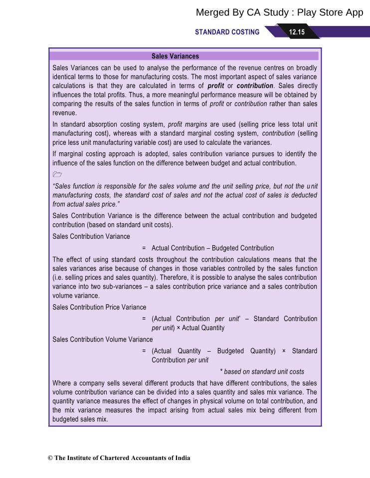
STANDARD COSTING 12.15
Sales Variances
Sales Variances can be used to analyse the performance of the revenue centres on broadly
identical terms to those for manufacturing costs. The most important aspect of sales variance
calculations is that they are calculated in terms of profit or contribution. Sales directly
influences the total profits. Thus, a more meaningful performance measure will be obtained by
comparing the results of the sales function in terms of profit or contribution rather than sales
revenue.
In standard absorption costing system, profit margins are used (selling price less total unit
manufacturing cost), whereas with a standard marginal costing system, contribution (selling
price less unit manufacturing variable cost) are used to calculate the variances.
If marginal costing approach is adopted, sales contribution variance pursues to identify the
influence of the sales function on the difference between budget and actual contribution.
“Sales function is responsible for the sales volume and the unit selling price, but not the u nit
manufacturing costs, the standard cost of sales and not the actual cost of sales is deducted
from actual sales price.”
Sales Contribution Variance is the difference between the actual contribution and budgeted
contribution (based on standard unit costs).
Sales Contribution Variance
= Actual Contribution – Budgeted Contribution
The effect of using standard costs throughout the contribution calculations means that the
sales variances arise because of changes in those variables controlled by the sales function
(i.e. selling prices and sales quantity). Therefore, it is possible to analyse the sales contribution
variance into two sub-variances – a sales contribution price variance and a sales contribution
volume variance.
Sales Contribution Price Variance
= (Actual Contribution per unit* – Standard Contribution
per unit) × Actual Quantity
Sales Contribution Volume Variance
= (Actual Quantity – Budgeted Quantity) × Standard
Contribution per unit
* based on standard unit costs
Where a company sells several different products that have different contributions, the sales
volume contribution variance can be divided into a sales quantity and sales mix variance. The
quantity variance measures the effect of changes in physical volume on to tal contribution, and
the mix variance measures the impact arising from actual sales mix being different from
budgeted sales mix.
© The Institute of Chartered Accountants of India
Merged By CA Study : Play Store App
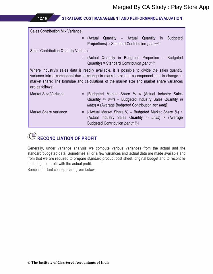
12.16 STRATEGIC COST MANAGEMENT AND PERFORMANCE EVALUATION
Sales Contribution Mix Variance
= (Actual Quantity – Actual Quantity in Budgeted
Proportions) × Standard Contribution per unit
Sales Contribution Quantity Variance
= (Actual Quantity in Budgeted Proportion – Budgeted
Quantity) × Standard Contribution per unit
Where industry’s sales data is readily available, it is possible to divide the sales quantity
variance into a component due to change in market size and a component due to change in
market share: The formulae and calculations of the market size and market share variances
are as follows:
Market Size Variance = [Budgeted Market Share % × (Actual Industry Sales
Quantity in units – Budgeted Industry Sales Quantity in
units) × (Average Budgeted Contribution per unit)]
Market Share Variance = [(Actual Market Share % – Budgeted Market Share %) ×
(Actual Industry Sales Quantity in units) × (Average
Budgeted Contribution per unit)]
RECONCILIATION OF PROFIT
Generally, under variance analysis we compute various variances from the actual and the
standard/budgeted data. Sometimes all or a few variances and actual data are made available and
from that we are required to prepare standard product cost sheet, original budget and to reconcile
the budgeted profit with the actual profit.
Some important concepts are given below:
© The Institute of Chartered Accountants of India
Merged By CA Study : Play Store App

STANDARD COSTING 12.17
Reconciliation Statement-I
Budgeted Profit to Actual Profit (Absorption Costing)
Budgeted Profit
(Budgeted Quantity × Standard Margin)
❑
Effect of Variances
Material Cost Variance
Material Price Variance ❑
Material Usage Variance
Material Mix Variance ❑
Material Yield Variance ❑ ❑ ❑
Labour Cost Variance
Labour Rate Variance ❑
Labour Idle Time Variance ❑
Labour Efficiency Variance
Labour Mix Variance ❑
Labour Sub-Efficiency Variance ❑ ❑ ❑
Variable Overhead Cost Variances
Variable Overhead Expenditure Variance ❑
Variable Overhead Efficiency Variance ❑ ❑
Fixed Overhead Cost Variances
Fixed Overhead Expenditure Variance ❑
Fixed Overhead Volume Variance
Fixed Overhead Capacity Variance ❑
Fixed Overhead Efficiency Variance ❑ ❑ ❑
Sales Margin Variances (in terms of Profit)
Sales Margin Price Variance ❑
Sales Margin Volume Variance
Sales Margin Mix Variance ❑
Sales Margin Quantity Variance ❑ ❑ ❑ ❑
Actual Profit ❑
© The Institute of Chartered Accountants of India
Merged By CA Study : Play Store App

12.18 STRATEGIC COST MANAGEMENT AND PERFORMANCE EVALUATION
Reconciliation Statement-II
Budgeted Profit to Actual Profit (Marginal Costing)
Budgeted Profit
(Budgeted Quantity × Standard Margin)
❑
Effect of Variances
Material Cost Variance
Material Price Variance ❑
Material Usage Variance
Material Mix Variance ❑
Material Yield Variance ❑ ❑ ❑
Labour Cost Variance
Labour Rate Variance ❑
Labour Idle Time Variance ❑
Labour Efficiency Variance
Labour Mix Variance ❑
Labour Sub-Efficiency Variance ❑ ❑ ❑
Variable Overhead Cost Variances
Variable Overhead Expenditure Variance ❑
Variable Overhead Efficiency Variance ❑ ❑
Fixed Overhead Cost Variances
Fixed Overhead Expenditure Variance ❑
Fixed Overhead Volume Variance
Fixed Overhead Capacity Variance NA
Fixed Overhead Efficiency Variance NA NA ❑
Sales Contribution Variances
Sales Contribution Price Variance ❑
Sales Contribution Volume Variance
Sales Contribution Mix Variance ❑
Sales Contribution Quantity Variance ❑ ❑ ❑ ❑
Actual Profit ❑
© The Institute of Chartered Accountants of India
Merged By CA Study : Play Store App

STANDARD COSTING 12.19
Reconciliation Statement-III
Standard Profit to Actual Profit (Absorption Costing)
Standard Profit
(Actual Quantity × Standard Margin)
❑
Effect of Variances
Material Cost Variance
Material Price Variance ❑
Material Usage Variance
Material Mix Variance ❑
Material Yield Variance ❑ ❑ ❑
Labour Cost Variance
Labour Rate Variance ❑
Labour Idle Time Variance ❑
Labour Efficiency Variance
Labour Mix Variance ❑
Labour Sub-Efficiency Variance ❑ ❑ ❑
Variable Overhead Cost Variances
Variable Overhead Expenditure Variance ❑
Variable Overhead Efficiency Variance ❑ ❑
Fixed Overhead Cost Variances
Fixed Overhead Expenditure Variance ❑
Fixed Overhead Volume Variance
Fixed Overhead Capacity Variance ❑
Fixed Overhead Efficiency Variance ❑ ❑ ❑
Sales Margin Variance (in terms of Profit)
Sales Margin Price Variance ❑
Sales Margin Volume Variance
Sales Margin Mix Variance NA
Sales Margin Quantity Variance NA NA ❑ ❑
Actual Profit ❑
© The Institute of Chartered Accountants of India
Merged By CA Study : Play Store App
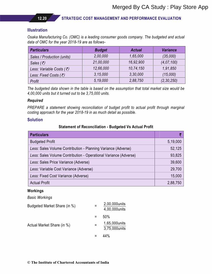
12.20 STRATEGIC COST MANAGEMENT AND PERFORMANCE EVALUATION
Illustration
Osaka Manufacturing Co. (OMC) is a leading consumer goods company. The budgeted and actual
data of OMC for the year 2018-19 are as follows-
Particulars Budget Actual Variance
Sales / Production (units) 2,00,000 1,65,000 (35,000)
Sales (`) 21,00,000 16,92,900 (4,07,100)
Less: Variable Costs (`) 12,66,000 10,74,150 1,91,850
Less: Fixed Costs (`) 3,15,000 3,30,000 (15,000)
Profit 5,19,000 2,88,750 (2,30,250)
The budgeted data shown in the table is based on the assumption that total market size would be 4,00,000 units but it turned out to be 3,75,000 units.
Required
PREPARE a statement showing reconciliation of budget profit to actual profit through marginal costing approach for the year 2018-19 in as much detail as possible.
Solution
Statement of Reconciliation - Budgeted Vs Actual Profit
Particulars `
Budgeted Profit 5,19,000
Less: Sales Volume Contribution - Planning Variance (Adverse) 52,125
Less: Sales Volume Contribution - Operational Variance (Adverse) 93,825
Less: Sales Price Variance (Adverse) 39,600
Less: Variable Cost Variance (Adverse) 29,700
Less: Fixed Cost Variance (Adverse) 15,000
Actual Profit 2,88,750
Workings
Basic Workings
Budgeted Market Share (in %) = 2,00,000units
4,00,000units
= 50%
Actual Market Share (in %) = 1,65,000units
3,75,000units
= 44%
© The Institute of Chartered Accountants of India
Merged By CA Study : Play Store App
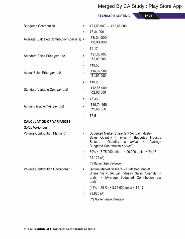
STANDARD COSTING 12.21
Budgeted Contribution = `21,00,000 – `12,66,000
= `8,34,000
Average Budgeted Contribution (per unit) = 8,34,000
2,00,000
`
`
= `4.17
Standard Sales Price per unit = 21,00,000
2,00,000
`
`
= `10.50
Actual Sales Price per unit = 16,92,900
1,65,000
`
`
= `10.26
Standard Variable Cost per unit = 12,66,000
2,00,000
`
`
= `6.33
Actual Variable Cost per unit = 10,74,150
1,65,000
`
`
= `6.51
CALCULATION OF VARIANCES
Sales Variances
Volume Contribution Planning* = Budgeted Market Share % × (Actual Industry Sales Quantity in units – Budgeted Industry Sales Quantity in units) × (Average Budgeted Contribution per unit)
= 50% × (3,75,000 units – 4,00,000 units) × `4.17
= 52,125 (A)
(*) Market Size Variance
Volume Contribution Operational** = (Actual Market Share % – Budgeted Market Share %) × (Actual Industry Sales Quantity in units) × (Average Budgeted Contribution per unit)
= (44% – 50 %) × 3,75,000 units × `4.17
= 93,825 (A)
(**) Market Share Variance
© The Institute of Chartered Accountants of India
Merged By CA Study : Play Store App
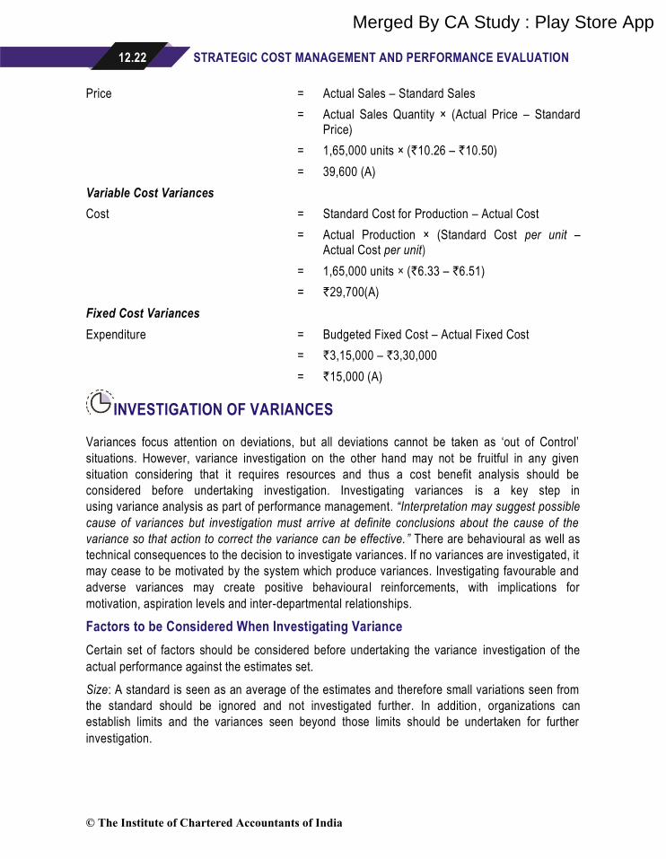
12.22 STRATEGIC COST MANAGEMENT AND PERFORMANCE EVALUATION
Price = Actual Sales – Standard Sales
= Actual Sales Quantity × (Actual Price – Standard Price)
= 1,65,000 units × (`10.26 – `10.50)
= 39,600 (A)
Variable Cost Variances
Cost = Standard Cost for Production – Actual Cost
= Actual Production × (Standard Cost per unit – Actual Cost per unit)
= 1,65,000 units × (`6.33 – `6.51)
= `29,700(A)
Fixed Cost Variances
Expenditure = Budgeted Fixed Cost – Actual Fixed Cost
= `3,15,000 – `3,30,000
= `15,000 (A)
INVESTIGATION OF VARIANCES
Variances focus attention on deviations, but all deviations cannot be taken as ‘out of Control’
situations. However, variance investigation on the other hand may not be fruitful in any given
situation considering that it requires resources and thus a cost benefit analysis should be
considered before undertaking investigation. Investigating variances is a key step in
using variance analysis as part of performance management. “Interpretation may suggest possible
cause of variances but investigation must arrive at definite conclusions about the cause of the
variance so that action to correct the variance can be effective.” There are behavioural as well as
technical consequences to the decision to investigate variances. If no variances are investigated, it
may cease to be motivated by the system which produce variances. Investigating favourable and
adverse variances may create positive behavioural reinforcements, with implications for
motivation, aspiration levels and inter-departmental relationships.
Factors to be Considered When Investigating Variance
Certain set of factors should be considered before undertaking the variance investigation of the
actual performance against the estimates set.
Size: A standard is seen as an average of the estimates and therefore small variations seen from
the standard should be ignored and not investigated further. In addition , organizations can
establish limits and the variances seen beyond those limits should be undertaken for further
investigation.
© The Institute of Chartered Accountants of India
Merged By CA Study : Play Store App

STANDARD COSTING 12.23
Type of Variance: Adverse variance is given more importance by the organization over favourable
variances seen with regards to the estimates.
Cost: The costs associated with the undertaking of the investigation should be lower than the
benefits associated with the investigation of variances for the organization to undertaken the said
investigation.
Pattern in variance: The variances need to be monitored over a period of time and if the variance
of a particular cost is seen to be worsening over time then in that case the investigation in relation
to the variance needs to be undertaken.
Budgetary process: In case the budgetary process is uncontrollable and unrealistic then in that
case the investigation should be re-evaluating the budgetary process rather than undertaking
investigation of the variances.
Method Used for Investing Variance1
Simple Rule of Thumb Model
It is based on arbitrary criteria such as investigating if the absolute size of a variance is greater
than a certain amount or if the ratio of the variance to the total cost exceeds some predetermined
percentage. They are based on managerial judgement and do not consider statistical significance.
Statistical Decision Model
For the statistical models, two mutually exclusive states are possible. First assumes that the
system is 'In Control' and a variance is simply due to random fluctuations around the expected
outcome. The second possible state is that the system is in some way 'Out of Control' and
corrective action can be taken to remedy the situation.
An investigation is undertaken when the probability that an observation comes from an ‘In -
Control’ distribution falls below some arbitrarily determined probability level.
A number of cost variance investigation models have been proposed that determine the statistical
probability that a variance comes from an ‘In Control’ distribution.
Determining Probabilities
'In Control' state can be stated in the form of a known probability distribution such as a normal one.
Let’s take example, consider a situation where the standard time required for a particular project
has been derived from the average of a series of past experience made under 'close' supervision.
The average time is 2.5 hrs. per unit of output. We shall consider that the actual observations were
normally distributed with a standard deviation of 15 minutes. Suppose that the actual time taken
for a week was 3,000 hrs. for output of 1,000 units. Thus, average time taken was 3 hrs. per unit of
output. We can determine the probability of perceiving an average time of 3 hrs. or more when the
process is under control through application of normal distribution theory. An observation of an
average time taken of 3 hrs. per unit of output is 2 standard deviations from the expected value,
where, for a normal distribution,
© The Institute of Chartered Accountants of India
Merged By CA Study : Play Store App

12.24 STRATEGIC COST MANAGEMENT AND PERFORMANCE EVALUATION
Probability of Completing the Project in 3 hrs.
Z = x –
σ
Z = 3.00 2.50
0.25
−
Z = 2.0
P (Z = 2.0) = 0.9772
Probability of Completing the Project in more than 3 hrs.
P = 1 - 0.9772
= 0.0228
The shaded area illustrates that 0.0228 of the area under the curve ( +2σ). Thus, the probability
of actual time taken per unit of output being 3 hrs. or more when the operation is under control is
2.28%.
It is likely that this observation comes from another distribution and that the time taken for the
week is out of control.
Statistical Control Charts
Statistical quality control is used mainly for monitoring and maintaining of the quality
of products and services, but within a standard costing framework, statistical control charts can be
used to monitor accounting variances. For example, labour usage could be plotted on a control
chart on an hourly basis for each project. This process would consist of sampling the output from a
project and plotting on the chart the mean usage of resources per unit for the sample output.
A control chart is a graphic presentation of a series of past observations in which each observation
is plotted relative to pre-set points on the expected distribution. Only observations beyond
specified pre-set control / tolerance limits are considered for investigation. The control limits are
set based on a series of past observations of a process when it is under control, and thus working
efficiently. It is assumed that the past observations can be represented by a normal distribution.
© The Institute of Chartered Accountants of India
Merged By CA Study : Play Store App

STANDARD COSTING 12.25
The past observations are used to estimate the population mean and the population standard
deviation σ. Assuming that the distribution of possible outcomes is normal, then, when the process
is under control, we should expect
68.27% of the observations to fall within the range + σ from the mean;
95.45% of the observations to fall within the range + 2σ from the mean;
99.8% of the observations to fall within the range + 3σ from the mean.
For example, if control limits are set based on 2σ from the mean then this would show 4.55%
(100% - 95.45%) of future observations would result from pure chance when the process is under
control. Therefore, there is a high probability that an observation outside the 2 σ control limits is out
of control.
Above Figure shows three control charts, with the outer horizontal lines representing a possible
control limit of 2σ, so that all observations outside this range are investigated.
For Project A the process is deemed to be in control because all observations fall within the control
limits.
For Project B the last two observations suggest that the project is out of control. Therefore, both
observations should be investigated.
With Project C, the observations would not prompt an investigation because all the observations
are within the control limits. However, the last six observations show a gradually increasing usage
in excess of the mean, and the process may be out of control. Statistical procedures that consider
the trend in recent usage as well as daily usage can also be used.
Statistical decision models have been extended to incorporate the costs and benefits of
investigation.
Decision rule to investigate if
PB > C
© The Institute of Chartered Accountants of India
Merged By CA Study : Play Store App

12.26 STRATEGIC COST MANAGEMENT AND PERFORMANCE EVALUATION
Where,
P is the probability that the process is ‘Out of Control’
B is the benefit associated with returning the process to its 'In-Control' state if the process is ‘Out
of Control’. Benefit represents the cost saving that will arise through bringing the system back
under control and thereby avoiding variances in future periods.
C is the cost will be incurred when an investigation is undertaken and includes the manager's
time spent on investigation, the cost of interrupting the production process, and the cost of
correcting the process. C is known with certainty.
The model requires an estimate of P, the probability that the process is ‘Out of Control’. Bierman
et al. (1961) have suggested that the probabilities could be determined by computing the
probability that a particular observation, such as a variance, comes from an 'In Co ntrol'
distribution. It also considers that the 'In- Control' state can be expressed in the form of a known
probability distribution such as a normal distribution.
Let us assume that the incremental cost of investigating the labour efficiency variance in our
example is `25. Assume also that the estimated benefit B from investigating a variance and
taking corrective action is `100.
Investigate if
P > 25/ 100 or 0.25
Consider our example, the probability of an observation of 3 hrs (or larger) was 0.0228. The
probability of the process being ‘Out of Control’ is one minus the probability of being ‘In Control’.
Thus, P = 0.9772 (1 - 0.0228). We ascertained that the variance should be investigated if the
probability that the process is ‘Out of Control’ is > 0.25. The process should therefore be
investigated.
1 Reference: Management and Cost Accounting by Colin M. Drury
POSSIBLE INTERDEPENDENCE BETWEEN VARIANCES
It is a term used to express the way in which the cause of one variance may be wholly or partially
explained by the cause of another variance. For control purposes, it might therefore be essential to
look at several variances together and not in isolation.
Some examples of interdependence between variances are listed below:
▪ Use of cheaper material which is poorer quality, the material price variance will be favourable,
but this can cause more wastage of materials leading to adverse usage variance.
▪ Using more skilled labour to do the work will result in an adverse labour rate variance, but
productivity might be higher as a result due to experienced labour.
© The Institute of Chartered Accountants of India
Merged By CA Study : Play Store App
STANDARD COSTING 12.27
▪ Changing the composition of a team might result in a cheaper labour mix (favourable mix
variance) but lower productivity (adverse yield variance).
▪ Workers trying to improve productivity (favourable efficiency variance) in order to get bonus
(adverse rate variance) might use materials wastefully in order to save time (adverse
materials usage).
▪ Cutting sales prices (adverse sales price variance) might result in higher sales demand from
customers (favourable sales volume variance).
▪ Similarly, favourable sales price variance may result in adverse sales volume variance.
INTERPRETATION OF VARIANCES
There can be a number of potential causes leading to variances in the operational costs
Material Price Variance
▪ Might be caused due to the use of a different supplier.
▪ Order size can result in variance.
▪ Any form of unexpected increase in buying costs such as higher delivery charges.
▪ Efficiency or inefficiency associated with the buying procedure adopted.
▪ Lack of appropriate inventory control can result in emergency purchase of material resulting
in adverse variance.
Material Usage Variance
▪ Purchase of inferior quality material.
▪ Implementation of better quality control.
▪ Increased efficiency in production can help in bringing down wastage rate.
▪ Changes made in the material mix.
▪ Careless way of handling material by production department.
▪ Change in method of production/ design.
▪ Pilferage of material from the production department.
▪ Poor inspection.
Labour Rate Variance
▪ Unexpected increase in the pay rate of labour.
© The Institute of Chartered Accountants of India
Merged By CA Study : Play Store App

12.28 STRATEGIC COST MANAGEMENT AND PERFORMANCE EVALUATION
▪ Level of experience of the labour can impact the direct cost of labour.
▪ Payment of bonuses added to the direct labour costs.
▪ Change in the composition of the workforce can impact direct labour costs.
Labour Efficiency Variance
▪ Improvement in work or productivity efficiency.
▪ Workforce mix can have an impact upon labour efficiency levels.
▪ Industrial action in relation to workforce.
▪ Poor supervision of the workforce.
▪ Learning curve effect upon the labour efficiency levels.
▪ Resource shortages causing an unexpected delay and lowering of labour efficiency levels.
▪ Using inferior quality of material.
▪ Introduction of new machinery resulting in improvement of labour productivity levels.
Overhead Variances
▪ Fixed Overhead Expenditure Variance (adverse) are caused by spending in excess of the
budget.
▪ Fixed Overhead Volume Variance is caused by changes in production volume.
▪ Variable Overhead Expenditure Variance are often caused by changes in machine running
costs.
▪ Variable Overhead Efficiency Variances- Causes are similar to those for a direct labour
efficiency variance.
Sales Price Variance
▪ Higher discounts given to customers in order to encourage bulk purchases.
▪ The effect of low price offers during a marketing campaign.
▪ Poor performance by sales personnel.
▪ Market conditions or economic conditions forcing changes in prices across the industry.
Sales Volume Variance
▪ Successful or unsuccessful direct selling efforts.
▪ Successful or unsuccessful marketing efforts (for example, the effects of an advertising
campaign).
▪ Unexpected changes in customer preferences and buying patterns.
© The Institute of Chartered Accountants of India
Merged By CA Study : Play Store App
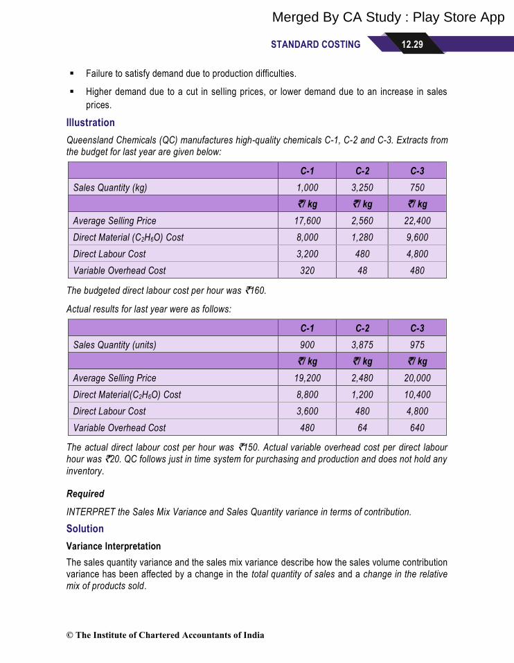
STANDARD COSTING 12.29
▪ Failure to satisfy demand due to production difficulties.
▪ Higher demand due to a cut in selling prices, or lower demand due to an increase in sales
prices.
Illustration
Queensland Chemicals (QC) manufactures high-quality chemicals C-1, C-2 and C-3. Extracts from the budget for last year are given below:
C-1 C-2 C-3
Sales Quantity (kg) 1,000 3,250 750
`/ kg `/ kg `/ kg
Average Selling Price 17,600 2,560 22,400
Direct Material (C2H6O) Cost 8,000 1,280 9,600
Direct Labour Cost 3,200 480 4,800
Variable Overhead Cost 320 48 480
The budgeted direct labour cost per hour was `160.
Actual results for last year were as follows:
C-1 C-2 C-3
Sales Quantity (units) 900 3,875 975
`/ kg `/ kg `/ kg
Average Selling Price 19,200 2,480 20,000
Direct Material(C2H6O) Cost 8,800 1,200 10,400
Direct Labour Cost 3,600 480 4,800
Variable Overhead Cost 480 64 640
The actual direct labour cost per hour was `150. Actual variable overhead cost per direct labour hour was `20. QC follows just in time system for purchasing and production and does not hold any
inventory.
Required
INTERPRET the Sales Mix Variance and Sales Quantity variance in terms of contribution.
Solution
Variance Interpretation
The sales quantity variance and the sales mix variance describe how the sales volume contribution variance has been affected by a change in the total quantity of sales and a change in the relative mix of products sold.
© The Institute of Chartered Accountants of India
Merged By CA Study : Play Store App

12.30 STRATEGIC COST MANAGEMENT AND PERFORMANCE EVALUATION
From the figures arrived for the sales quantity contribution variance, we can observe that the increase in total quantity sold would have gained an additional contribution of `2,124,600, if the
actual sales volume had been in the budgeted sales proportion.
The sales mix contribution variance shows that the variation in the sales mix resulted in a curtailment in profit by `570,600. The change in the sales mix has resulted in a relatively higher
proportion of sales of C-2 which is the chemical that earns the lowest contribution and a lower proportion of C-1 which earn a contribution significantly higher. The relative increase in the sale of C-3 however, which has the highest unit contribution, has partially offset the switch in mix to C-2.
Workings
Statement Showing Standard Contribution
C-1
`/ kg
C-2
`/ kg
C-3
`/ kg
Average Selling Price 17,600 2,560 22,400
Direct Material (C2H6O) Cost 8,000 1,280 9,600
Direct Labour Cost 3,200 480 4,800
Variable Overhead Cost 320 48 480
Contribution 6,080 752 7,520
Sales Contribution Mix Variance
Pro
du
cts
Actual Quantity
[AQ]
Actual Sales at Budgeted Proportion
[RAQ]
Difference
[AQ – RAQ]
Contribution
`
[SC]
Mix Variance
(`’ 000)
SC × [AQ – RAQ]
C-1 900 1,150 250 (A) 6,080 1,520 (A)
C-2 3,875 3,737.50 137.50 (F) 752 103.40 (F)
C-3 975 862.50 112.50 (F) 7,520 846 (F)
5,750 5,750 570.60 (A)
Sales Contribution Quantity Variance
Pro
du
cts
Budget Sales
Quantity
[BQ]
Actual Sales at Budgeted Proportion
[RAQ]
Difference
[RAQ – 𝐁𝐐]
Contribution
`
[SC]
Qty. Variance
(`’ 000)
SC × [RAQ – BQ]
C-1 1,000 1,150 150 (F) 6,080 912 (F)
C-2 3,250 3,737.50 487.50 (F) 752 366.60 (F)
C-3 750 862.50 112.50 (F) 7,520 846 (F)
5,000 5,750 2,124.60 (F)
© The Institute of Chartered Accountants of India
Merged By CA Study : Play Store App

STANDARD COSTING 12.31
Case Scenario
Natural Spices manufactures and distributes high-quality spices to gourmet food shops and top
quality restaurants. Gourmet and high-end restaurants pride themselves on using the freshest,
highest-quality ingredients.
Natural Spices has set up five state of the art plants for meeting the ever- growing demand.
The firm procures raw material directly from the centers of produce to maintain uniform taste
and quality. The raw material is first cleaned, dried and tested with the help of special
machines. It is then carefully grounded into the finished product passing through various stages
and packaged at the firm’s ultraclean factory before being dispatched to customers.
The following variances pertain to last week of operations, arose as a consequence of
management’s decision to lower prices to increase volume.
Sales Volume Variance 18,000 (F)
Sales Price Variance 14,000 (A)
Purchase Price Variance 10,000 (F)
Labour Efficiency Variance 11,200 (F)
Fixed Cost Expenditure Variance 4,400 (F)
Required
(i) IDENTIFY the ‘Critical Success Factors’ for Natural Spices.
(ii) EVALUATE the management’s decision with the ‘Overall Corporate Strategy’ and ‘Critical
Success Factors’.
Solution
(i) Gourmet and high-end restaurants recognises Natural Spices on the basis of its high
quality of spices. Therefore, quality is most critical success factor of Natural Spices. There
are other factors which cannot be ignore such as price, delivery options, att ractive packing
etc. But all are secondary to the quality.
(ii) Deliberate action of cutting price to increase sales volume indicates that firm is intending
to expand its market to retail market and street shops which is price sensitive.
Purchase Price Variance is clearly indicating that firm has purchased raw material at lower
price which may be due to buying of lower quality of material. Similarly, positive Efficiency
Variance is indicating cost cutting and stretching resources.
It appears that firm is intending to expand its market to retail market and street shops by
not only reducing the price but also compromising its quality which is opposing its current
strategy of high quality.
Management should monitor the trends of variances on regular basis and take appropriate
action in case of evidence of permanent decline in quality. Here, customer feedback is
also very important.
© The Institute of Chartered Accountants of India
Merged By CA Study : Play Store App

12.32 STRATEGIC COST MANAGEMENT AND PERFORMANCE EVALUATION
REPORTING OF VARIANCES
Computation of variances and their reporting is not the final step towards the control of various elements of cost. It in fact demands an analysis of variances from the side of the executives, to ascertain the correct reasons for their occurrence. After knowing the exact reasons, it becomes their responsibility to take necessary steps so as to stop the re-occurrence of adverse variances in future. To enhance the utility of such a reporting system it is necessary that such a system of reporting should not only be prompt but should also facilitate the concerned managerial level to take necessary steps. Variance reports should be prepared after keeping in view its ultimate use and its periodicity. Such reports should highlight the essential cost deviations and possibilities for their improvements. In fact the variance reports should give due regard to the following points:-
(i) The concerned executives should be informed about what the cost performance should have been.
(ii) How close the actual cost performance is with reference to standard cost performance.
(iii) The analysis and causes of variances.
(iv) Reporting should be based on the principle of management by exception.
(v) The magnitude of variances should also be stated.
BEHAVIOURAL ISSUES
Variance analysis may encourage short-termism due to their inherent tendency towards short-term, quantified objectives and results.
A negative perception of an organization's variance analysis process can also encourage other sub-optimal behaviour among employees such as attempts to include budget slacks.
The behavioural issues connected with variance analysis could be managed by participating employees during budget setting so that they do not assess the procedure as biased. It is also vital for an organization's performance measurement system to be based on a extensive range of quantitative and qualitative measures so as to encourage management to adopt a long-term view that is aligned with an organization's strategic direction.
Source: Managerial Accounting: A Focus on Ethical Decision Making by Steve Jackson, Roby Sawyers, Greg Jenkins
Ethics
Variance analysis for evaluating performance can have strong ethical consequences. For
example, standard costing methods have been proposed for medicine as a means for
improving performance1. Interpretation of a favourable variance may be difficult because it
either reflects insufficient treatment or compliance to guidelines. Most hospitals in various
countries are reimbursed as specified by the diagnostic related groups (DRG). Each DRG has
specified standard “length of stay”. If a patient leaves the hospital early, the hospital is financial
impacted favourably but a patient staying longer than the specified time costs the hospital
money.
Source: 1- Cornerstones of Financial and Managerial Accounting (2011) by Jay Rich, Jeff Jones, Dan L. Heitger,
Maryanne Mowen, Don Hansen, Standard Costing: A Managerial Control Tool, p 1020.
© The Institute of Chartered Accountants of India
Merged By CA Study : Play Store App
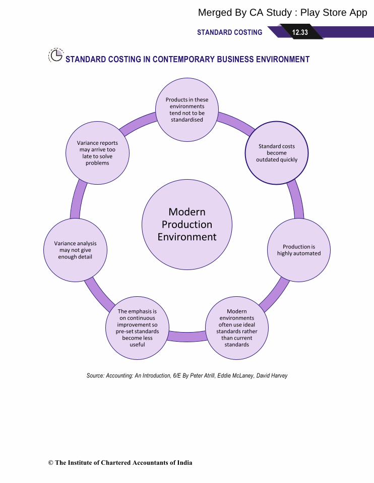
STANDARD COSTING 12.33
STANDARD COSTING IN CONTEMPORARY BUSINESS ENVIRONMENT
Source: Accounting: An Introduction, 6/E By Peter Atrill, Eddie McLaney, David Harvey
Modern Production
Environment
Products in these environments tend not to be standardised
Standard costs become
outdated quickly
Production is highly automated
Modern environments often use ideal
standards rather than current
standards
The emphasis is on continuous
improvement so pre-set standards
become less useful
Variance analysis may not give enough detail
Variance reports may arrive too
late to solve problems
© The Institute of Chartered Accountants of India
Merged By CA Study : Play Store App

12.34 STRATEGIC COST MANAGEMENT AND PERFORMANCE EVALUATION
FORMULAE
© The Institute of Chartered Accountants of India
Merged By CA Study : Play Store App
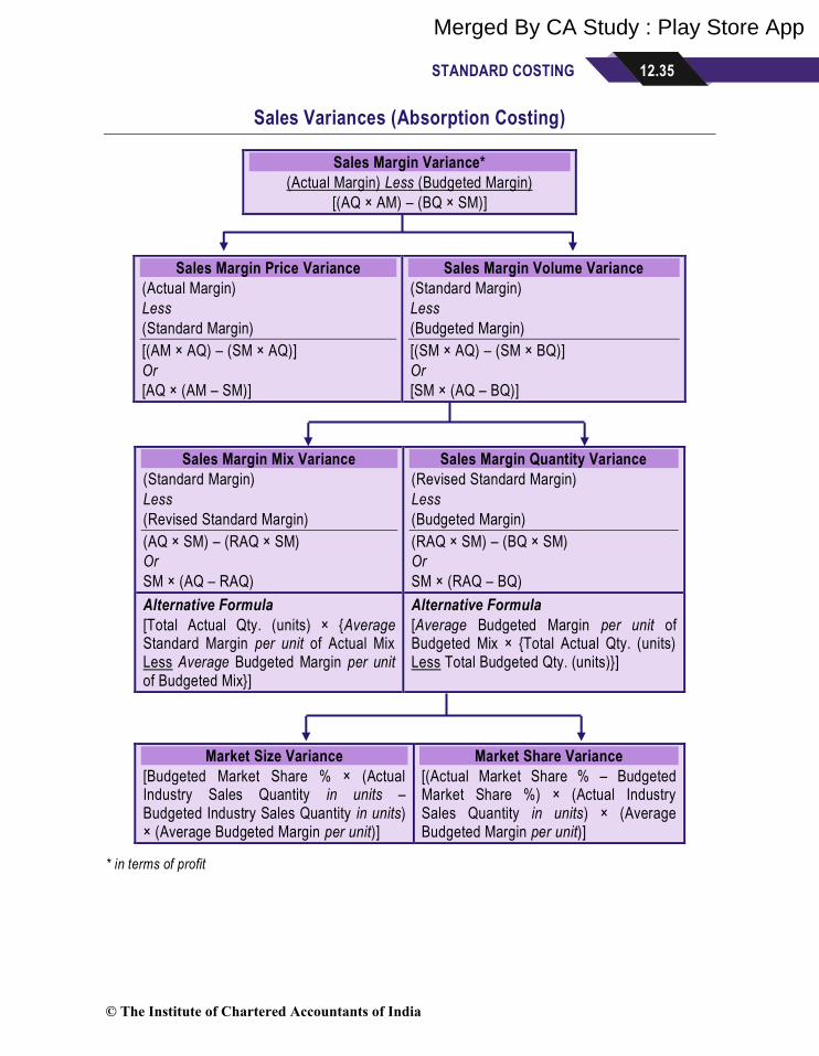
STANDARD COSTING 12.35
Sales Variances (Absorption Costing)
Sales Margin Variance*
(Actual Margin) Less (Budgeted Margin)
[(AQ × AM) – (BQ × SM)]
* in terms of profit
Sales Margin Price Variance
(Actual Margin)
Less
(Standard Margin)
[(AM × AQ) – (SM × AQ)]
Or
[AQ × (AM – SM)]
Sales Margin Volume Variance
(Standard Margin)
Less
(Budgeted Margin)
[(SM × AQ) – (SM × BQ)]
Or
[SM × (AQ – BQ)]
Sales Margin Mix Variance
(Standard Margin)
Less
(Revised Standard Margin)
(AQ × SM) – (RAQ × SM)
Or
SM × (AQ – RAQ)
Sales Margin Quantity Variance
(Revised Standard Margin)
Less
(Budgeted Margin)
(RAQ × SM) – (BQ × SM)
Or
SM × (RAQ – BQ)
Alternative Formula
[Total Actual Qty. (units) × {Average Standard Margin per unit of Actual Mix Less Average Budgeted Margin per unit of Budgeted Mix}]
Alternative Formula
[Average Budgeted Margin per unit of Budgeted Mix × {Total Actual Qty. (units) Less Total Budgeted Qty. (units)}]
Market Size Variance
[Budgeted Market Share % × (Actual Industry Sales Quantity in units – Budgeted Industry Sales Quantity in units) × (Average Budgeted Margin per unit)]
Market Share Variance
[(Actual Market Share % – Budgeted Market Share %) × (Actual Industry Sales Quantity in units) × (Average Budgeted Margin per unit)]
© The Institute of Chartered Accountants of India
Merged By CA Study : Play Store App

12.36 STRATEGIC COST MANAGEMENT AND PERFORMANCE EVALUATION
Note:
BQ = Budgeted Sales Quantity
AQ = Actual Sales Quantity
RAQ = Revised Actual Sales Quantity
= Actual Quantity Sold Rewritten in Budgeted Proportion
SM = Standard Margin
= Standard Price per Unit – Standard Cost per Unit
AM = Actual Margin
= Actual Sales Price per Unit – Standard Cost per Unit
Market Size Variance
Budgeted Market Share % × (Actual Industry Sales Quantity in units – Budgeted Industry Sales Quantity in units) × (Average Budgeted Margin per unit)
Or
(Budgeted Market Share % × Actual Industry Sales Quantity in units – Budgeted Market Share % × Budgeted Industry Sales Quantity in units) × (Average Budgeted Margin per unit)
Or
(Required Sales Quantity in units –Total Budgeted Quantity in units) × (Average Budgeted Margin per unit)
Market Share Variance
(Actual Market Share % – Budgeted Market Share %) × (Actual Industry Sales Quantity in units) × (Average Budgeted Margin per unit)
Or
(Actual Market Share % × Actual Industry Sales Quantity in units – Budgeted Market Share % × Actual Industry Sales Quantity in units) × (Average Budgeted Margin per unit)
Or
(Total Actual Quantity in units– Required Sales Quantity in units) × (Average Budgeted Margin per unit)
Market Size Variance + Market Share Variance
(Required Sales Quantity in units – Total Budgeted Quantity in units) × (Average Budgeted Margin per unit)
Add
(Total Actual Quantity in units– Required Sales Quantity in units) × (Average Budgeted Margin per unit)
Equals to
(Total Actual Quantity in units – Total Budgeted Quantity in units) × (Average Budgeted Margin per unit)
Sales Margin Quantity Variance
© The Institute of Chartered Accountants of India
Merged By CA Study : Play Store App
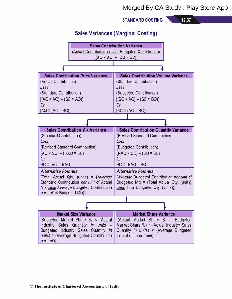
STANDARD COSTING 12.37
Sales Variances (Marginal Costing)
Sales Contribution Variance
(Actual Contribution) Less (Budgeted Contribution)
[(AQ × AC) – (BQ × SC)]
Sales Contribution Price Variance
(Actual Contribution)
Less
(Standard Contribution)
[(AC × AQ) – (SC × AQ)]
Or
[AQ × (AC – SC)]
Sales Contribution Volume Variance
(Standard Contribution)
Less
(Budgeted Contribution)
[(SC × AQ) – (SC × BQ)]
Or
[SC × (AQ – BQ)]
Sales Contribution Mix Variance
(Standard Contribution)
Less
(Revised Standard Contribution)
(AQ × SC) – (RAQ × SC)
Or
SC × (AQ – RAQ)
Sales Contribution Quantity Variance
(Revised Standard Contribution)
Less
(Budgeted Contribution)
(RAQ × SC) – (BQ × SC)
Or
SC × (RAQ – BQ)
Alternative Formula
[Total Actual Qty. (units) × {Average Standard Contribution per unit of Actual Mix Less Average Budgeted Contribution per unit of Budgeted Mix}]
Alternative Formula
[Average Budgeted Contribution per unit of Budgeted Mix × {Total Actual Qty. (units) Less Total Budgeted Qty. (units)}]
Market Size Variance
[Budgeted Market Share % × (Actual Industry Sales Quantity in units – Budgeted Industry Sales Quantity in units) × (Average Budgeted Contribution per unit)]
Market Share Variance
[(Actual Market Share % – Budgeted Market Share %) × (Actual Industry Sales Quantity in units) × (Average Budgeted Contribution per unit)]
© The Institute of Chartered Accountants of India
Merged By CA Study : Play Store App

12.38 STRATEGIC COST MANAGEMENT AND PERFORMANCE EVALUATION
Note:
BQ = Budgeted Sales Quantity
AQ = Actual Sales Quantity
RAQ = Revised Actual Sales Quantity
= Actual Quantity Sold Rewritten in Budgeted Proportion
SC = Standard Contribution
= Standard Price per Unit – Standard Cost (variable) per Unit
AC = Actual Contribution
= Actual Sales Price per Unit – Standard Cost (variable) per Unit
Market Size Variance
Budgeted Market Share % × (Actual Industry Sales Quantity in units – Budgeted Industry Sales Quantity in units) × (Average Budgeted Contribution per unit)
Or
(Budgeted Market Share % × Actual Industry Sales Quantity in units – Budgeted Market Share % × Budgeted Industry Sales Quantity in units) × (Average Budgeted Contribution per unit)
Or
(Required Sales Quantity in units – Total Budgeted Quantity in units) × (Average Budgeted Contribution per unit)
Market Share Variance
(Actual Market Share % – Budgeted Market Share %) × (Actual Industry Sales Quantity in units) × (Average Budgeted Contribution per unit)
Or
(Actual Market Share % × Actual Industry Sales Quantity in units – Budgeted Market Share % × Actual Industry Sales Quantity in units) × (Average Budgeted Contribution per unit)
Or
(Total Actual Quantity in units– Required Sales Quantity in units) × (Average Budgeted Contribution per unit)
Market Size Variance + Market Share Variance
(Required Sales Quantity in units – Total Budgeted Quantity in units) × (Average Budgeted Contribution per unit)
Add
(Total Actual Quantity in units– Required Sales Quantity in units) × (Average Budgeted Contribution per unit)
Equals to
(Total Actual Quantity in units – Total Budgeted Quantity in units) × (Average Budgeted Contribution per unit)
Sales Contribution Quantity Variance
© The Institute of Chartered Accountants of India
Merged By CA Study : Play Store App

STANDARD COSTING 12.39
▪ Sales Price Variance is equal to Sales Margin/ Contribution Price Variance. This is
because, for the actual quantity sold, standard cost remaining constant, change in selling
price will have equal impact or turnover and profit/ contribution.
▪ Sales Margin Volume Variance is equal to Sales Volume Variance × Budgeted Net Profit
Ratio
▪ Sales Contribution Volume Variance is equal to Sales Volume Variance × Budgeted PV
Ratio
A Relation: Sales Margin Volume Variance in terms of Profit & Contribution
Sales Margin Volume Variance Standard Margin Per Unit × (Actual Quantity −
Budgeted Quantity)
Or
Sales Margin Volume Variance [Standard Contribution Per Unit − Standard Fixed
Overheads Per Unit] × (Actual Quantity −
Budgeted Quantity)
Or
Sales Margin Volume Variance [Standard Contribution Per Unit × (Actual
Quantity − Budgeted Quantity)] − [Standard Fixed
Overheads Per Unit × (Actual Quantity −
Budgeted Quantity)]
Or
Sales Margin Volume Variance Sales Contribution Volume Variance − Fixed
Overhead Volume Variance
Or
Sales Contribution Volume Variance
Sales Margin Volume Variance + Fixed Overhead
Volume Variance
Note: Production units equals to Sales units for both actual & budget.
© The Institute of Chartered Accountants of India
Merged By CA Study : Play Store App

12.40 STRATEGIC COST MANAGEMENT AND PERFORMANCE EVALUATION
Sales Variances (Turnover or Value)
Sales Variance
(Actual Sales) Less (Budgeted Sales)
[(AQ × AP) – (BQ × SP)]
Sales Price Variance
(Actual Sales)
Less
(Standard Sales)
[(AP × AQ) – (SP × AQ)]
Or
[AQ × (AP – SP)]
Sales Volume Variance
(Standard Sales)
Less
(Budgeted Sales)
[(SP × AQ) – (SP × BQ)]
Or
[SP × (AQ – BQ)]
Sales Mix Variance
(Standard Sales)
Less
(Revised Standard Sales)
[(SP × AQ) – (SP × RAQ)]
Or
[SP × (AQ – RAQ)]
Sales Quantity Variance
(Revised Standard Sales)
Less
(Budgeted Sales)
[(SP × RAQ) – (SP × BQ)]
Or
[SP × (RAQ – BQ)]
Alternative Formula
[Total Actual Quantity (units) × {Average Standard Price per unit of Actual Mix Less Average Budgeted Price per unit of Budgeted Mix}]
Alternative Formula
[Average Budgeted Price per unit of Budgeted Mix × {Total Actual Quantity (units) Less Total Budgeted Qty (units)}]
Market Size Variance
[Budgeted Market Share % × (Actual Industry Sales Quantity in units – Budgeted Industry Sales Quantity in units) × (Average Budgeted Price per unit)]
Market Share Variance
[(Actual Market Share % – Budgeted Market Share %) × (Actual Industry Sales Quantity in units) × (Average Budgeted Price per unit)]
© The Institute of Chartered Accountants of India
Merged By CA Study : Play Store App

STANDARD COSTING 12.41
Note:
BQ = Budgeted Sales Quantity
AQ = Actual Sales Quantity
RAQ = Revised Actual Sales Quantity
= Actual Quantity Sold Rewritten in Budgeted Proportion
SP = Standard Selling Price per Unit
AP = Actual Selling Price per Unit
Market Size Variance
Budgeted Market Share % × (Actual Industry Sales Quantity in units – Budgeted Industry Sales Quantity in units) × (Average Budgeted Price per unit)
Or
(Budgeted Market Share % × Actual Industry Sales Quantity in units – Budgeted Market Share % × Budgeted Industry Sales Quantity in units) × (Average Budgeted Price per unit)
Or
(Required Sales Quantity in units –Total Budgeted Quantity in units) × (Average Budgeted Price per unit)
Market Share Variance
(Actual Market Share % – Budgeted Market Share %) × (Actual Industry Sales Quantity in units) × (Average Budgeted Price per unit)
Or
(Actual Market Share % × Actual Industry Sales Quantity in units – Budgeted Market Share % × Actual Industry Sales Quantity in units) × (Average Budgeted Price per unit)
Or
(Total Actual Quantity in units– Required Sales Quantity in units) × (Average Budgeted Price per unit)
Market Size Variance + Market Share Variance
(Required Sales Quantity in units – Total Budgeted Quantity in units) × (Average Budgeted Price per unit)
Add
(Total Actual Quantity in units– Required Sales Quantity in units) × (Average Budgeted Price per unit)
Equals to
(Total Actual Quantity in units – Total Budgeted Quantity in units) × (Average Budgeted Price per unit)
Sales Quantity Variance
© The Institute of Chartered Accountants of India
Merged By CA Study : Play Store App

12.42 STRATEGIC COST MANAGEMENT AND PERFORMANCE EVALUATION
Direct Material Variances
Direct Material Total Variance#
[Standard Cost* – Actual Cost]
(The difference between the Standard Direct Material Cost of the actual
production volume and the Actual Cost of Direct Material)
[(SQ × SP) – (AQ × AP)]
Direct Material Price Variance
[Standard Cost of Actual Quantity – Actual Cost]
(The difference between the Standard Price
and Actual Price for the Actual Quantity)
[(SP – AP) × AQ]
Or
[(SP × AQ) – (AP × AQ)]
Direct Material Usage Variance
[Standard Cost of Standard Quantity for Actual Production – Standard Cost of Actual Quantity]
(The difference between the Standard Quantity
specified for actual production and the Actual
Quantity used, at Standard Purchase Price)
[(SQ – AQ) × SP]
Or
[(SQ × SP) – (AQ × SP)]
Direct Material Mix Variance
[Standard Cost of Actual Quantity in Standard Proportion – Standard Cost of Actual Quantity]
(The difference between the Actual Quantity in
standard proportion and Actual Quantity in actual
proportion, at Standard Purchase Price)
[(RAQ – AQ) × SP]
Or
[(RAQ × SP) – (AQ × SP)]
Direct Material Yield Variance
[Standard Cost of Standard Quantity for Actual Production – Standard Cost of Actual Quantity in Standard Proportion]
(The difference between the Standard Quantity
specified for actual production and Actual Quantity
in standard proportion, at Standard Purchase
Price)
[(SQ – RAQ) × SP]
Or
[(SQ × SP) – (RAQ × SP)]
Alternative Formula
[Total Actual Quantity (units) × {Average Standard Price per unit of Standard Mix Less Average Standard Price per unit of Actual Mix}]
Alternative Formula
[Average Standard Price per unit of Standard Mix × {Total Standard Quantity (units) Less Total Actual Quantity (units)}]
© The Institute of Chartered Accountants of India
Merged By CA Study : Play Store App

STANDARD COSTING 12.43
Note:
SQ = Standard Quantity = Expected Consumption for Actual Output
AQ = Actual Quantity of Material Consumed
RAQ = Revised Actual Quantity = Actual Quantity Rewritten in Standard Proportion
SP = Standard Price per Unit
AP = Actual Price per Unit
(*) = Standard Cost refers to ‘Standard Cost of Standard Quantity for Actual Output’
(#) = Direct Material Total Variance (also known as material cost variance)
Material Purchase Price Variance
[Standard Cost of Actual Quantity – Actual Cost]
(The difference between the Standard Price and Actual Price
for the actual quantity of material purchased)
[(SP – AP) × PQ]
Or
[(SP × PQ) – (AP × PQ)]
Note:
PQ = Purchase Quantity
SP = Standard Price
AP = Actual Price
© The Institute of Chartered Accountants of India
Merged By CA Study : Play Store App

12.44 STRATEGIC COST MANAGEMENT AND PERFORMANCE EVALUATION
Direct Labour Variances
Direct Labour Total Variance1
[Standard Cost2 – Actual Cost]
(The difference between the Standard Direct Labour Cost and the Actual
Direct Labour Cost incurred for the production achieved)
[(SH × SR) – (AH* × AR)]
Direct Labour
Rate Variance
[Standard Cost of Actual Time – Actual Cost]
(The difference between the
Standard Rate per hour and Actual
Rate per hour for the Actual Hours
paid)
[(SR – AR) × AH*]
Or
[(SR × AH*) – (AR × AH*)]
Direct Labour
Idle Time Variance
[Standard Rate per Hour × Actual Idle Hours]
(The difference between the Actual
Hours paid and Actual Hours
worked at Standard Rate)
[(AH* – AH#) × SR]
Or
[(AH* × SR) – (AH# × SR)]
Direct Labour
Efficiency Variance
[Standard Cost of Standard Time for Actual Production – Standard Cost of Actual Time]
(The difference between the
Standard Hours specified for
actual production and Actual Hours
worked at Standard Rate)
[(SH – AH#) × SR]
Or
[(SH × SR) – (AH# × SR)]
Direct Labour Mix Variance
Or Gang Variance
[Standard Cost of Actual Time Worked in Standard Proportion – Standard Cost of Actual Time Worked]
(The difference between the Actual Hours worked in
standard proportion and Actual Hours worked in actual
proportion, at Standard Rate)
[(RAH – AH#) × SR]
Or
[(RAH × SR) – (AH# × SR)]
Direct Labour Yield Variance
Or Sub-Efficiency Variance
[Standard Cost of Standard Time for Actual Production – Standard Cost of Actual Time Worked in Standard Proportion]
(The difference between the Standard Hours
specified for actual production and Actual Hours
worked in standard proportion, at Standard Rate)
(SH – RAH) × SR
Or
(SH × SR) – (RAH × SR)
Alternate Formula
[Total Actual Time Worked (hours) × {Average Standard Rate per hour of Standard Gang Less Average Standard Rate per hour of Actual Gang@}] @ on the basis of hours worked
Alternate Formula
[Average Standard Rate per hour of Standard Gang × {Total Standard Time (hours) Less Total Actual Time Worked (hours)}]
© The Institute of Chartered Accountants of India
Merged By CA Study : Play Store App

STANDARD COSTING 12.45
Note:
SH = Standard Hours = Expected time (Time allowed) for Actual Output
AH* = Actual Hours paid for
AH# = Actual Hours worked
RAH = Revised Actual Hours = Actual Hours (worked) rewritten in Standard Proportion
SR = Standard Rate per Labour Hour
AR = Actual Rate per Labour Hour Paid
(2) = Standard Cost refers to ‘Standard Cost of Standard Time for Actual Output’
(1) = Direct Labour Total Variance (also known as labour cost variance)
In the absence of idle time
Actual Hours Worked = Actual Hours Paid
Idle Time is a period for which a workstation is available for production but is not used due to e.g.
shortage of tooling, material, or operators. During Idle Time, Direct Labour Wages are being paid
but no output is being produced. The cost of this can be identified separately in an Idle Time
Variance, so that it is not ‘hidden’ in an adverse Labour Efficiency Variance.
Some organizations face Idle Time on regular basis. In this situation, the Standard Labour Rate
may include an allowance for the cost of the expected idle time. Only the impact of any
unexpected or abnormal Idle Time would be included in the Idle Time Variance.
© The Institute of Chartered Accountants of India
Merged By CA Study : Play Store App
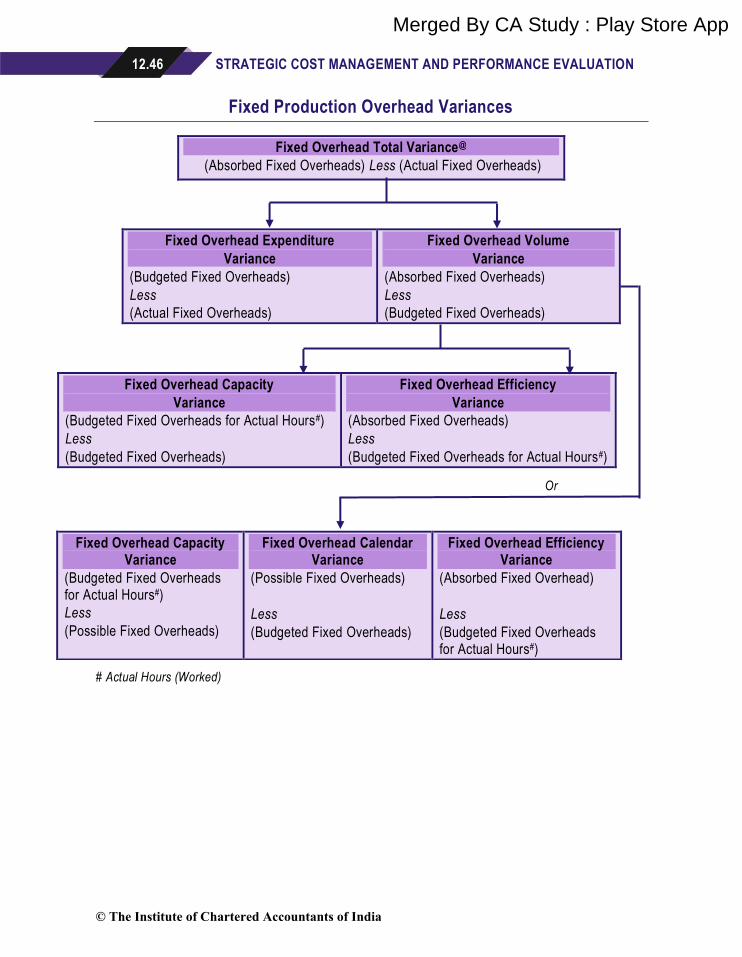
12.46 STRATEGIC COST MANAGEMENT AND PERFORMANCE EVALUATION
Fixed Production Overhead Variances
Fixed Overhead Total Variance@
(Absorbed Fixed Overheads) Less (Actual Fixed Overheads)
Fixed Overhead Expenditure
Variance
(Budgeted Fixed Overheads)
Less
(Actual Fixed Overheads)
Fixed Overhead Volume
Variance
(Absorbed Fixed Overheads)
Less
(Budgeted Fixed Overheads)
Fixed Overhead Capacity
Variance
(Budgeted Fixed Overheads for Actual Hours#)
Less
(Budgeted Fixed Overheads)
Fixed Overhead Efficiency
Variance
(Absorbed Fixed Overheads)
Less
(Budgeted Fixed Overheads for Actual Hours#)
# Actual Hours (Worked)
Fixed Overhead Capacity Variance
(Budgeted Fixed Overheads for Actual Hours#)
Less
(Possible Fixed Overheads)
Fixed Overhead Calendar Variance
(Possible Fixed Overheads)
Less
(Budgeted Fixed Overheads)
Fixed Overhead Efficiency Variance
(Absorbed Fixed Overhead)
Less
(Budgeted Fixed Overheads for Actual Hours#)
Or
© The Institute of Chartered Accountants of India
Merged By CA Study : Play Store App

STANDARD COSTING 12.47
Note:
Standard Fixed Overheads for Production (Absorbed)
= Standard Fixed Overhead Rate per Unit × Actual Production in Units
= Standard Fixed Overhead Rate per Hour × Standard Hours for Actual Production
Budgeted Fixed Overheads
= It represents the amount of fixed overhead which should be spent according to the budget or
standard during the period
= Standard Fixed Overhead Rate per Unit × Budgeted Production in Units
= Standard Fixed Overhead Rate per Hour × Budgeted Hours
Actual Fixed Overheads Incurred
Budgeted Fixed Overheads for Actual Hours
= Standard Fixed Overhead Rate per Hour × Actual Hours
Possible Fixed Overheads
= Expected Fixed Overhead for Actual Days Worked
= Budgeted Fixed Overhead
Budgeted Days× Actual Days
(@)
= Fixed Overhead Total Variance also known as ‘Fixed Overhead Cost Variance’
Fixed Overhead Efficiency Variance
(Absorbed Fixed Overheads) – (Budgeted Fixed Overheads for Actual Hours)
Or
(Standard Fixed Overhead Rate per Hour × Standard Hours for Actual Output) – (Standard Fixed Overhead Rate per Hour × Actual Hours)
Or
Standard Fixed Overhead Rate per Hour × (Standard Hours for Actual Output – Actual Hours)
Fixed Overhead Capacity Variance
(Budgeted Fixed Overheads for Actual Hours) – (Budgeted Fixed Overheads)
Or
(Standard Fixed Overhead Rate per Hour × Actual Hours) – (Standard Fixed Overhead Rate per Hour × Budgeted Hours)
Or
Standard Fixed Overhead Rate per Hour × (Actual Hours – Budgeted Hours)
© The Institute of Chartered Accountants of India
Merged By CA Study : Play Store App

12.48 STRATEGIC COST MANAGEMENT AND PERFORMANCE EVALUATION
Fixed Overhead Volume Variance-I
(Absorbed Fixed Overheads) – (Budgeted Fixed Overheads)
Or
(Standard Fixed Overhead Rate per Unit × Actual Output) – (Standard Fixed Overhead Rate per Unit × Budgeted Output)
Or
Standard Fixed Overhead Rate per Unit × (Actual Output – Budgeted Output)
Fixed Overhead Volume Variance-II
(Absorbed Fixed Overheads) – (Budgeted Fixed Overheads)
Or
(Standard Fixed Overhead Rate per Hour × Standard Hours for Actual Output) – (Standard Fixed Overhead Rate per Hour × Budgeted Hours)
Or
Standard Fixed Overhead Rate per Hour × (Standard Hours for Actual Output – Budgeted Hours)
Or
Standard Fixed Overhead Rate per Hour × (Standard Hours per Unit × Actual Output – Standard Hours per Unit × Budgeted Output)
Or
(Standard Fixed Overhead Rate per Hour × Standard Hours per Unit) × (Actual Output – Budgeted Output)
Or
Standard Fixed Overhead Rate per Unit × (Actual Output – Budgeted Output)
Overhead Variances can also be affected by idle time. It is usually assumed that Overheads are
incurred when labour is working, not when it is idle. Accordingly, hours worked has been
considered for the calculation of Variable and Fixed Overheads Variances.
© The Institute of Chartered Accountants of India
Merged By CA Study : Play Store App

STANDARD COSTING 12.49
Variable Production Overhead Variances
Variable Overhead Total Variance@
(Standard Variable Overheads for Production – Actual Variable Overheads)
# Actual Hours (Worked)
Note:
Standard Variable Overheads for Production/Charged to Production
= Standard/Budgeted Variable Overhead Rate per Unit × Actual Production (Units)
= Standard Variable Overhead Rate per Hour × Standard Hours for Actual Production
Actual Overheads Incurred
Budgeted Variable Overheads for Actual Hours
= Standard Variable Overhead Rate per Hour × Actual Hours
(@)
= Variable Overhead Total Variance also known as ‘Variable Overhead Cost Variance’
Variable Overhead Efficiency Variance
(Standard Variable Overheads for Production) – (Budgeted Overheads for Actual Hours)
Or
(Standard Variable Overhead Rate per Hour × Standard Hours for Actual Output) – (Standard Variable Overhead Rate per Hour × Actual Hours)
Or
Standard Variable Overhead Rate per Hour × (Standard Hours for Actual Output – Actual hours)
Variable Overhead Expenditure Variance
(Budgeted Variable Overheads for Actual Hours) – (Actual Variable Overheads)
Or
(Standard Rate per Hour × Actual Hours) – (Actual Rate per Hour × Actual Hours)
Or
Actual Hours × (Standard Rate per Hour – Actual Rate per Hour)
Variable Overhead Expenditure (Spending) Variance
(Budgeted Variable Overheads for Actual Hours#)
Less
(Actual Variable Overheads)
Variable Overhead
Efficiency Variance
(Standard Variable Overheads for Production)
Less
(Budgeted Variable Overheads for Actual Hours#)
© The Institute of Chartered Accountants of India
Merged By CA Study : Play Store App

12.50 STRATEGIC COST MANAGEMENT AND PERFORMANCE EVALUATION
SUMMARY
▪ Planning & Operational Variances- A Planning Variance simply compares a revised
standard to the original standard.
An Operational Variance simply compares the actual results against the revised amount.
Operating variances would be calculated after the planning variances have been established
and are thus a realistic way of assessing performance.
Controllable Variances are those variances which arises due to inefficiency of a cost centre
/department. Uncontrollable Variances are those variances which arises due to factors
beyond the control of the management or concerned department of the organization.
▪ Variance Analysis in Activity Based Costing - Variance analysis can be applied to activity
costs (such as setup costs) to gain insight into why actual activity costs differ from activity
costs in the static budget or in the flexible budget. Interpreting cost variances for different
activates requires understanding whether the costs are output unit-level, batch level, product
sustaining, or facility sustaining costs.
▪ Variance Analysis in Advanced Manufacturing Environment/ High Technology Firms -
In the high-technology environment, large part of manufacturing process is computerized.
Many costs that once were largely variable have become fixed, most becoming committed
fixed cost. Some high technology manufacturing organizations have found that the two
largest variable costs involve materials and power to operate machines. In these companies,
the emphasis of variance analysis is placed on direct materials and variable manufacturing
overhead. For these firms labour variances may no longer be meaningful because direct
labour is a committed cost, not a cost expected to vary with output.
▪ Impact of Learning Curve - Learning curve is a geometrical progression, which reveals that
there is steadily decreasing cost for the accomplishment of a given repetitive operation, as
the identical operation is increasingly repeated. The amount of decrease will be less and less
with each successive unit produced. Automated manufacturing is unlikely to have much
variation or to display a regular learning curve. In less-automated processes, however, where
learning curves do occur, it is important to take the resulting decline in labour hours and costs
into account in setting standards, determining prices, planning production, or setting up work
schedules.
▪ Investigation of Variances - An investigation should only be undertaken if the benefits
expected from the investigation exceeds the costs of searching for and correcting the source
of the variance. Interpretation may suggest possible cause of variances but investigation
must arrive at definite conclusions about the cause of the variance so that action to correct
the variance can be effective.
© The Institute of Chartered Accountants of India
Merged By CA Study : Play Store App

STANDARD COSTING 12.51
▪ Relevant Cost Approach to Variance Analysis is used if inputs are limited. Failure to use
limited inputs properly leads not only to increased acquisition cost but also to a lost
contribution. Therefore, it is necessary to consider the lost contribution in variance analysis.
When this approach is used, price or expenditure variances are not affected.
▪ Standard Costing in Service Sector -Use of activity based costing can provide a
constructive basis for variance analysis of overheads in service sector organizations.
▪ McDonaldization – Breaking tasks into smallest possible units and rationalising them to find
the single most efficient method for completing each task. All other tasks are discard ed.
standards can be more accurately set and assessed. Helpful in services like hairdressing,
dentistry, or opticians' services.
▪ Behavioural Issues of Standard Costing– Focus on short term, sub-optimal behaviour of
the employees like incorporation of budget slacks. These issues can be overcome by
involving employees in budget preparation and taking a long- term view of organisation
strategy incorporating various qualitative and quantitative measures .
▪ Possible Interdependence between Variances – Using cheaper materials will result in a
favourable material price variance, but using the cheaper material in production might
increase the wastage rate (adverse material usage) and cause a fall in labour productivity
(adverse labour and variable overhead efficiency). A more expensive mix of materials
(adverse mix variance) might result in higher output yields (favourable yield variance).
Using more experienced labour to do the work will result in an adverse labour rate variance,
but productivity might be higher as a result (favourable labour and variable overhead
efficiency).
▪ Standard costing may be inappropriate in the modern production environment because:
products may not be standardised, get outdated quickly, automation of production, emphasis
on continuous improvement, delay in problem solving.
© The Institute of Chartered Accountants of India
Merged By CA Study : Play Store App
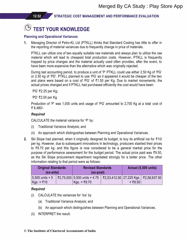
12.52 STRATEGIC COST MANAGEMENT AND PERFORMANCE EVALUATION
TEST YOUR KNOWLEDGE
Planning and Operational Variances
1. Managing Director of Petro-KL Ltd (PTKLL) thinks that Standard Costing has little to offer in the reporting of material variances due to frequently change in price of materials.
PTKLL can utilize one of two equally suitable raw materials and always plan to utilize the raw material which will lead to cheapest total production costs. However, PTKLL is frequently trapped by price changes and the material actually used often provides, after the event, to have been more expensive than the alternative which was originally rejected.
During last accounting period, to produce a unit of ‘P’ PTKLL could use either 2.50 Kg of ‘PG’ or 2.50 kg of ‘PD’. PTKLL planned to use ‘PG’ as it appeared it would be cheaper of the two and plans were based on a cost of ‘PG’ of `1.50 per Kg. Due to market movements, the actual prices changed and if PTKLL had purchased efficiently the cost would have been:
‘PG’ `2.25 per Kg;
‘PD’ `2.00 per Kg
Production of ‘P’ was 1,000 units and usage of ‘PG’ amounted to 2,700 Kg at a total cost of ` 6,480/-
Required
CALCULATE the material variance for ‘P’ by:
(i) Traditional Variance Analysis; and
(ii) An approach which distinguishes between Planning and Operational Variances.
2. Ski Slope had planned, when it originally designed its budget, to buy its artificial ice for `10/
per kg. However, due to subsequent innovations in technology, producers slashed their prices
to `9.70 per kg. and this figure is now considered to be a general market price for the
purpose of performance assessment for the budget period. The actual price paid was `9.50,
as the Ski Slope procurement department negotiated strongly for a better price. The other
information relating to that period were as follows:
Original Standards
(ex-ante)
Revised Standards
(ex-post)
Actual (5,500 units)
5,500 units × 5
Kgs. × `10
`2,75,000 5,500 units × 4.75
Kgs. × `9.70
`2,53,412.50 27,225 Kgs.
× `9.50
`2,58,637.50
Required
(i) CALCULATE the variances for ‘Ice’ by
(a) Traditional Variance Analysis; and
(b) An approach which distinguishes between Planning and Operational Variances.
(ii) INTERPRET the result.
© The Institute of Chartered Accountants of India
Merged By CA Study : Play Store App

STANDARD COSTING 12.53
3. KONY Ltd., based in Kuala Lumpur, is the Malaysian subsidiary of Japan's NY corporation, headquartered in Tokyo. KONY's principal Malaysian businesses include marketing, sales, and after-sales service of electronic products & software exports products. KONY set up a new factory in Penang to manufacture and sell integrated circuit ‘Q50X-N’. The first quarter’s budgeted production and sales were 2,000 units. The budgeted sales price and standard costs for ‘Q50X-N’ were as follows:
RM RM
Standard Sales Price per unit 50
Standard Costs per unit
Circuit X (10 units @ RM 2.5) 25
Circuit Designers (6 hrs. @ RM 2) 12 (37)
Standard Contribution per unit 13
Actual results for the first quarter were as follows:
RM ’000 RM ’000
Sales (2,000 units) 158
Production Costs (2,000 units)
Circuit X (21,600 units) 97.20
Circuit Designers (11,600 hours) 34.80 (132)
Actual Contribution (2,000 units) 26
The management accountant made the following observations on the actual results –
“In total, the performance agreed with budget; however, in every aspect other than volume, there were huge differences. Sales were made at what was supposed to be the highest feasible price, but we now feel that we could have sold for RM 82.50 with no adverse effect on volume. The Circuit X cost that was anticipated at the time the budget was prepared was RM 2.5 per unit. However, the general market price relating to efficient purchases of the Circuit X during the quarter was RM 4.25 per unit. Circuit designers have the responsibility of designing electronic circuits that make up electrical systems. Circuit Designer’s costs rose dramatically with increased demand for the specialist skills required to produce the ‘Q50X-N’, and the general market rate was RM 3.125 per hour - although KONY always paid below the normal market rate whenever possible. In my opinion, it is not necessary to measure the first quarter’s performance through variance analysis. Further, our operations are fully efficient as the final contribution is equal to the original budget.”
Required
COMMENT on management accountant’s view.
© The Institute of Chartered Accountants of India
Merged By CA Study : Play Store App
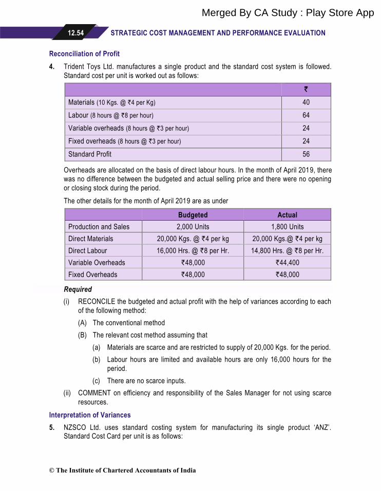
12.54 STRATEGIC COST MANAGEMENT AND PERFORMANCE EVALUATION
Reconciliation of Profit
4. Trident Toys Ltd. manufactures a single product and the standard cost system is followed.
Standard cost per unit is worked out as follows:
`
Materials (10 Kgs. @ `4 per Kg) 40
Labour (8 hours @ `8 per hour) 64
Variable overheads (8 hours @ `3 per hour) 24
Fixed overheads (8 hours @ `3 per hour) 24
Standard Profit 56
Overheads are allocated on the basis of direct labour hours. In the month of April 2019, there
was no difference between the budgeted and actual selling price and there were no opening
or closing stock during the period.
The other details for the month of April 2019 are as under
Budgeted Actual
Production and Sales 2,000 Units 1,800 Units
Direct Materials 20,000 Kgs. @ `4 per kg 20,000 Kgs.@ `4 per kg
Direct Labour 16,000 Hrs. @ `8 per Hr. 14,800 Hrs. @ `8 per Hr.
Variable Overheads `48,000 `44,400
Fixed Overheads `48,000 `48,000
Required
(i) RECONCILE the budgeted and actual profit with the help of variances according to each
of the following method:
(A) The conventional method
(B) The relevant cost method assuming that
(a) Materials are scarce and are restricted to supply of 20,000 Kgs. for the period.
(b) Labour hours are limited and available hours are only 16,000 hours for the
period.
(c) There are no scarce inputs.
(ii) COMMENT on efficiency and responsibility of the Sales Manager for not using scarce
resources.
Interpretation of Variances
5. NZSCO Ltd. uses standard costing system for manufacturing its single product ‘ANZ’. Standard Cost Card per unit is as follows:
© The Institute of Chartered Accountants of India
Merged By CA Study : Play Store App

STANDARD COSTING 12.55
(`)
Direct Material (1 kg per unit) 20
Direct Labour (6 hrs @ `8 per hour) 48
Variable Overheads 24
Actual and Budgeted Activity Levels in units for the month of Feb’19 are:
Budget Actual
Production 50,000 52,000
Actual Variable Costs for the month of Feb’19 are given as under:
Direct Material 10,65,600
Direct Labour (3,00,000 hrs) 24,42,000
Variable Overheads 12,28,000
Required
INTERPRET Direct Labour Rate and Efficiency Variances.
6. T-tech is a Taiwan based firm, that designs, develops, and sells audio equipment. Founded in
1975 by Mr. Boss, firm sells its products throughout the world. T-tech is best known for its
home audio systems and speakers, noise cancelling headphones, professional audio
systems and automobile sound systems. Extracts from the budget are shown in the following
table:
Home Audio System Division
Jan’2019
System Sales (units) Selling Price
`
Standard Cost (per System) `
3,000 W PMPO 1,500 18,750 12,500
5,000 W PMPO 500 50,000 26,250
The Managing Director has sent you a copy of an email he received from the Sales Manager
‘K’. The content of the email was as follows:
“We have had an outstanding month. There was an adverse Sales Price Variance on the
3,000 W PMPO Systems of `22,50,000 but I compensated for that by raising the price of
5,000 W PMPO Systems. Unit sales of 3,000 W PMPO Systems were as expected but sales
of the 5,000 W PMPOs were exceptional and gave a Sales Margin Volume Variance of
`23,75,000. I think I deserve a bonus!”
The managing Director has asked for your opinion on these figures. You got the following
information:
© The Institute of Chartered Accountants of India
Merged By CA Study : Play Store App

12.56 STRATEGIC COST MANAGEMENT AND PERFORMANCE EVALUATION
Actual results for Jan’ 2019 were:
System Sales (units) Selling Price `
3,000 W PMPO 1,500 `17,250
5,000 W PMPO 600 `53,750
The total market demand for 3,000 W PMPO Systems was as budgeted but as a result of
suppliers reducing the price of supporting UHD TV System the total market for 5,000 W
PMPO Systems raised by 50% in Jan’2019.
The company had sufficient capacity to meet the revised market demand for 750 units of its
5,000 W PMPO Systems and therefore maintained its market share.
Required
(i) CALCULATE the following Operational Variances based on the revised market details:
- Sales Margin Mix Variance
- Sales Margin Volume Variance
(ii) COMMENT briefly on the measurement of the K’s performance.
ANSWERS/ SOLUTIONS
1. (i) Traditional Variances
Usage Variance = (2,500 Kg – 2,700 Kg) × `1.50
= `300 (A)
Price Variance = (`1.50 – `2.40) × 2,700 Kg
= `2,430 (A)
Total Variance = `300 (A) + `2,430 (A)
= `2,730 (A)
(ii) Operational Variances
Usage Variance = (2,500 Kg – 2,700 Kg) × `2.25
= `450 (A)
Price Variance = (`2.25 – `2.40) × 2,700 Kg
= `405 (A)
Total Variance = `450 (A) + `405 (A)
= `855 (A)
© The Institute of Chartered Accountants of India
Merged By CA Study : Play Store App
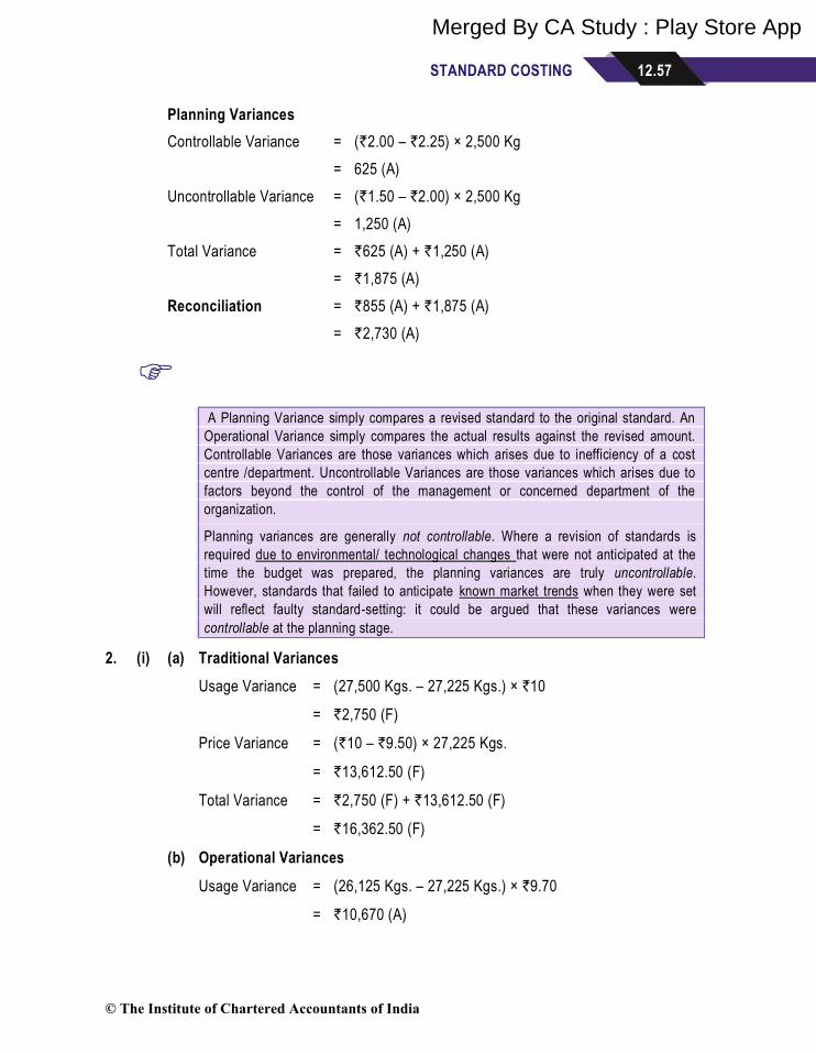
STANDARD COSTING 12.57
Planning Variances
Controllable Variance = (`2.00 – `2.25) × 2,500 Kg
= 625 (A)
Uncontrollable Variance = (`1.50 – `2.00) × 2,500 Kg
= 1,250 (A)
Total Variance = `625 (A) + `1,250 (A)
= `1,875 (A)
Reconciliation = `855 (A) + `1,875 (A)
= `2,730 (A)
A Planning Variance simply compares a revised standard to the original standard. An
Operational Variance simply compares the actual results against the revised amount.
Controllable Variances are those variances which arises due to inefficiency of a cost
centre /department. Uncontrollable Variances are those variances which arises due to
factors beyond the control of the management or concerned department of the
organization.
Planning variances are generally not controllable. Where a revision of standards is
required due to environmental/ technological changes that were not anticipated at the
time the budget was prepared, the planning variances are truly uncontrollable.
However, standards that failed to anticipate known market trends when they were set
will reflect faulty standard-setting: it could be argued that these variances were
controllable at the planning stage.
2. (i) (a) Traditional Variances
Usage Variance = (27,500 Kgs. – 27,225 Kgs.) × `10
= `2,750 (F)
Price Variance = (`10 – `9.50) × 27,225 Kgs.
= `13,612.50 (F)
Total Variance = `2,750 (F) + `13,612.50 (F)
= `16,362.50 (F)
(b) Operational Variances
Usage Variance = (26,125 Kgs. – 27,225 Kgs.) × `9.70
= `10,670 (A)
© The Institute of Chartered Accountants of India
Merged By CA Study : Play Store App
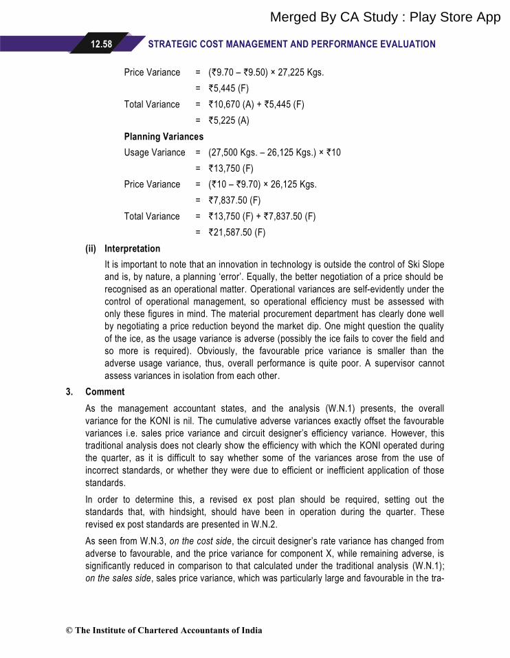
12.58 STRATEGIC COST MANAGEMENT AND PERFORMANCE EVALUATION
Price Variance = (`9.70 – `9.50) × 27,225 Kgs.
= `5,445 (F)
Total Variance = `10,670 (A) + `5,445 (F)
= `5,225 (A)
Planning Variances
Usage Variance = (27,500 Kgs. – 26,125 Kgs.) × `10
= `13,750 (F)
Price Variance = (`10 – `9.70) × 26,125 Kgs.
= `7,837.50 (F)
Total Variance = `13,750 (F) + `7,837.50 (F)
= `21,587.50 (F)
(ii) Interpretation
It is important to note that an innovation in technology is outside the control of Ski Slope
and is, by nature, a planning ‘error’. Equally, the better negotiation of a price should be
recognised as an operational matter. Operational variances are self-evidently under the
control of operational management, so operational efficiency must be assessed with
only these figures in mind. The material procurement department has clearly done well
by negotiating a price reduction beyond the market dip. One might question the quality
of the ice, as the usage variance is adverse (possibly the ice fails to cover the field and
so more is required). Obviously, the favourable price variance is smaller than the
adverse usage variance, thus, overall performance is quite poor. A supervisor cannot
assess variances in isolation from each other.
3. Comment
As the management accountant states, and the analysis (W.N.1) presents, the overall
variance for the KONI is nil. The cumulative adverse variances exactly offset the favourable
variances i.e. sales price variance and circuit designer’s efficiency variance. However, this
traditional analysis does not clearly show the efficiency with which the KONI operated during
the quarter, as it is difficult to say whether some of the variances arose from the use of
incorrect standards, or whether they were due to efficient or inefficient application of those
standards.
In order to determine this, a revised ex post plan should be required, setting out the
standards that, with hindsight, should have been in operation during the quarter. These
revised ex post standards are presented in W.N.2.
As seen from W.N.3, on the cost side, the circuit designer’s rate variance has changed from
adverse to favourable, and the price variance for component X, while remaining adverse, is
significantly reduced in comparison to that calculated under the traditional analysis (W.N.1);
on the sales side, sales price variance, which was particularly large and favourable in the tra-
© The Institute of Chartered Accountants of India
Merged By CA Study : Play Store App

STANDARD COSTING 12.59
ditional analysis (W.N.1), is changed into an adverse variance in the revised approach,
reflecting the fact that the KONI failed to sell at prices that were actually available in the
market.
Further, variances arose from changes in factors external to the business (W.N .4), which
might not have been known or acknowledged by standard-setters at the time of planning are
beyond the control of the operational managers. The distinction between variances is
necessary to gain a realistic measure of operational efficiency.
W.N.1
KONY India Ltd.
Quarter-1
Operating Statement
Particulars Favourable
RM
Adverse
RM
RM
Budgeted Contribution 26,000
Sales Price Variance [(RM 79 - RM 50) × 2,000 units] 58,000 ---
NIL
Circuit X Price Variance
[(RM 2.50 – RM 4.50) × 21,600 units]
43,200
Circuit X Usage Variance
[(20,000 units - 21,600 units) × RM 2.50]
4,000
Circuit Designer’s Rate Variance
[(RM 2 - RM 3) × 11,600 hrs.]
11,600
Circuit Designer’s Efficiency Variance
[(12,000 hrs. - 11,600 hrs.) × RM 2.00]
800
Actual Contribution 26,000
W.N.2
Statement Showing Original Standards, Revised Standards, and Actual Results for Quarter 1
Original Standards
(ex-ante)
Revised Standards
(ex-post)
Actual
Sales 2,000 units
× RM 50.00
RM 1,00,000 2,000 units
× RM 82.50
RM 1,65,000 2,000 units
× RM 79.00
RM 1,58,000
Circuit X 20,000 units
× RM 2.50
RM 50,000 20,000 units
× RM 4.25
RM 85,000 21,600 units
× RM 4.50
RM 97,200
Circuit
Designer
12,000 hrs.
× RM 2.00
RM 24,000 12,000 hrs.
× RM 3.125
RM 37,500 11,600 hrs.
× RM 3.00
RM 34,800
© The Institute of Chartered Accountants of India
Merged By CA Study : Play Store App

12.60 STRATEGIC COST MANAGEMENT AND PERFORMANCE EVALUATION
W.N.3
Statement Showing Operational Variances
Particulars (`) (`)
Operational Variances
16,500 (A)
Sales Price [(RM 79.00 - RM 82.50) × 2,000 units] 7,000 (A)
Circuit X Price [(RM 4.25 - RM 4.50) × 21,600 units] 5,400 (A)
Circuit X Usage [(20,000 units – 21,600 units) × RM 4.25] 6,800 (A)
Circuit Designer Rate [(RM 3.125 - RM 3.00) × 11,600 hrs.] 1,450 (F)
Circuit Designer Efficiency [(12,000 hrs.– 11,600 hrs.) × RM 3.125] 1,250 (F)
W.N.4
Statement Showing Planning Variances
Particulars (`) (`)
Planning Variance
16,500 (F) Sales Price [(RM 82.50 - RM 50.00) × 2,000 units] 65,000 (F)
Circuit X Price [(RM 2.50 - RM 4.25) × 20,000 units] 35,000 (A)
Circuit Designer Rate [(RM 2.00 - RM 3.125) × 12,000 hrs.] 13,500 (A)
4. (i) Computation of Variances
Material Usage Variance = Standard Price × (Standard Quantity – Actual Quantity)
= `4.00 × (18,000* Kgs. – 20,000 Kgs.)
= `8,000 (A)
*20,000 Kgs.
1,800 units2,000 units
Labour Efficiency Variance = Standard Rate × (Standard Hours – Actual Hours)
= `8.00 × (14,400* hrs. – 14,800 hrs.)
= `3,200 (A)
*16,000 hrs.
1,800 units2,000 units
Variable Overhead Efficiency Variance
= Standard Variable Overheads for Production – Budgeted Variable Overheads for Actual hours
© The Institute of Chartered Accountants of India
Merged By CA Study : Play Store App

STANDARD COSTING 12.61
= (14,400 hrs. × `3.00) – (`3.00 × 14,800 hrs.)
= `1,200 (A)
Fixed Overhead Volume Variance
= Absorbed Fixed Overheads – Budgeted Fixed Overheads
= (14,400 hrs. × `3.00) – (16,000 hrs. × `3.00)
= `4,800 (A)
Sales Margin Volume Variance
= Standard Margin – Budgeted Margin
= (1,800 units × `56.00) – (2,000 units × `56.00)
= `11,200 (A)
Sales Contribution Volume Variance
= Standard Contribution – Budgeted Contribution
= (1,800 units × `80.00) – (2,000 units × `80.00)
= `16,000 (A)
Statement Showing “Reconciliation Between Budgeted Profit & Actual Profit”
Particulars Conv. Method (`)
Relevant Cost Method (`)
Scarce Material
Scarce Labour
No Scarce Inputs
Budgeted Profit
(2,000 units × `56)
1,12,000 1,12,000 1,12,000 1,12,000
Sales Volume Variance 11,200 (A) NIL* 12,000$ (A) 16,000 (A)
Material Usage Variance 8,000 (A) 24,000 (A) 8,000 (A) 8,000 (A)
Labour Efficiency Variance 3,200 (A) 3,200 (A) 7,200 (A) 3,200 (A)
Variable Overhead Efficiency Variance
1,200 (A) 1,200 (A) 1,200 (A) 1,200 (A)
Fixed Overhead Volume Variance
4,800 (A) N.A.# N.A. # N.A. #
Actual Profit 83,600 83,600 83,600 83,600
© The Institute of Chartered Accountants of India
Merged By CA Study : Play Store App

12.62 STRATEGIC COST MANAGEMENT AND PERFORMANCE EVALUATION
Notes
Scarce Material
Based on conventional method, direct material usage variance is `8,000 (A) i.e. 2,000
Kg. × `4. In this situation material is scarce, and, therefore, material cost variance
based on relevant cost method should also include contribution lost per unit of material.
Excess usage of 2,000 Kg. leads to lost contribution of `16,000 i.e. 2,000 Kgs. × `8.
Total material usage variance based on relevant cost method, when material is
scarce will be: `8,000 (A) + `16,000 (A) = `24,000 (A). Since labour is not scarce,
labour variances are identical to conventional method.
Excess usage of 2,000 Kgs. leads to loss of contribution from 200 units i.e. `16,000
(200 units × `80). It is not the function of the sales manager to use material efficiently.
Hence, loss of contribution from 200 units should be excluded while computing sales
contribution volume variance.
(*)→
Therefore, sales contribution volume variance, when materials are scarce will be
NIL i.e. `16,000 (A) - `16,000 (A).
Scarce Labour
Material is no longer scarce, and, therefore, the direct material variances are same as in
conventional method. In conventional method, excess labour hours used are: 14,400
hrs. – 14,800 hrs. = 400 hrs. Contribution lost per hour = `10. Therefore, total
contribution lost, when labour is scarce will be: 400 hrs. × `10 = `4,000. Therefore,
total labour efficiency variance, when labour hours are scarce will be `7,200 (A)
i.e. `3,200 (A) + `4,000 (A).
Excess usage of 400 hrs. leads to loss of contribution from 50 units i.e. `4,000 (50 units
× `80). It is not the function of the sales manager to use labour hours efficiently. Hence,
loss of contribution from 50 units should be excluded while computing sales contribution
volume Variance.
($)→
Therefore, sales contribution volume variance, when labour hours are Scarce will
be `12,000 (A) i.e. `16,000 (A) - `4,000 (A).
Fixed Overhead Volume Variance
(#) →
The fixed overhead volume variance does not arise in marginal costing system. In
absorption costing system, it represents the value of the under or over absorbed fixed
overheads due to change in production volume. When marginal costing is in use there is
no overhead volume variance, because marginal costing does not absorb fixed
overheads.
© The Institute of Chartered Accountants of India
Merged By CA Study : Play Store App

STANDARD COSTING 12.63
(ii) Comment on Efficiency and Responsibility of the Sales Manager
In general, Gross Profit (or contribution margin) is the joint responsibility of sales
managers as well as of production managers. On one hand the sales manager is
responsible for the sales revenue part, on the other hand the production manager is
accountable for the cost-of-goods-sold component. However, it is the top management
who needs to ensure that the target profit is achieved by the organization. The sales
manager is accountable for prices, volume, and mix of the product, whereas the
production manager must control the costs of materials, labour, factory overheads and
quantities of production. The purchase manager must purchase materials at budgeted
prices. The personnel manager must employ right people at the right place with
appropriate wage rates. The internal audit manager must ensure that the budgetary
figures for sales and costs are being adhered by all departments which are directly or
indirectly involved in contribution of making profit. Thus, sales manager is not
responsible for contribution lost due to excess usage or inefficient usage of resources in
case of scarce resources. Hence, such contribution lost must be excluded from the sales
contribution volume variance.
5. Interpretation
Direct Labour Rate Variance
Adverse Labour Rate Variance indicates that the labour rate per hour paid is more than the
set standard. The reason may include among other things such as:
(1) While setting standard, the current/ future market conditions like pending labour
negotiation/ cases, has not been considered (or predicted) correctly.
(2) The labour may have been told that their wage rate will be raised or bonus will be paid if
they work efficiently.
Direct Labour Efficiency Variance
It indicates that the workers have produced actual production quantity in less time than the
time allowed. The reason for favourable labour efficiency variance may include among the
other things as follows:
(1) While setting standard, workers efficiency could not be estimated properly, this may
happen due to non-observance of time and motion study.
(2) The workers may be new in the factory, hence, efficiency could not be predicated
properly.
(3) The foreman or personnel manager responsible for labour efficiency, while providing his/
her input at the time of budget/ standard, has adopted conservative approach.
(4) The increase in the labour rate might have encouraged the labours to do work more
efficiently.
© The Institute of Chartered Accountants of India
Merged By CA Study : Play Store App
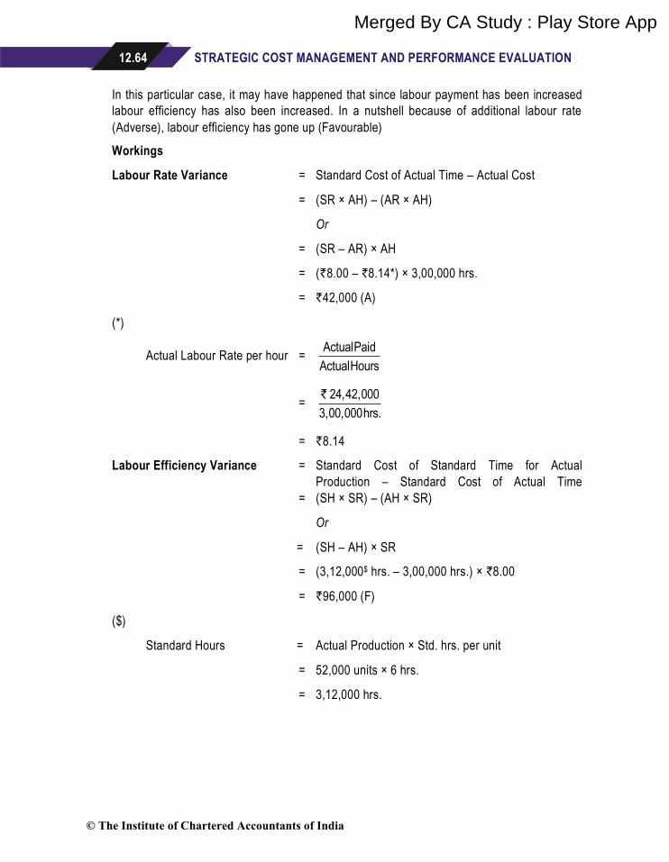
12.64 STRATEGIC COST MANAGEMENT AND PERFORMANCE EVALUATION
In this particular case, it may have happened that since labour payment has been increased
labour efficiency has also been increased. In a nutshell because of additional labour rate
(Adverse), labour efficiency has gone up (Favourable)
Workings
Labour Rate Variance = Standard Cost of Actual Time – Actual Cost
= (SR × AH) – (AR × AH)
Or
= (SR – AR) × AH
= (`8.00 – `8.14*) × 3,00,000 hrs.
= `42,000 (A)
(*)
Actual Labour Rate per hour = ActualPaid
ActualHours
= 24,42,000
3,00,000hrs.
= `8.14
Labour Efficiency Variance = Standard Cost of Standard Time for Actual
Production – Standard Cost of Actual Time
= (SH × SR) – (AH × SR)
Or
= (SH – AH) × SR
= (3,12,000$ hrs. – 3,00,000 hrs.) × `8.00
= `96,000 (F)
($)
Standard Hours = Actual Production × Std. hrs. per unit
= 52,000 units × 6 hrs.
= 3,12,000 hrs.
© The Institute of Chartered Accountants of India
Merged By CA Study : Play Store App

STANDARD COSTING 12.65
6. (i) Statement Showing Sales Margin Mix Variance
System
Standard Margin
per unit
(`)
Actual
Qty.
(units)
Revised Actual
Quantity
(units)
Difference
(`)
Variance
(`)
3,000 W PMPO 6,250 1,500 1,400 +100 +6,25,000 (F)
5,000 W PMPO 23,750 600 700 -100 23,75,000 (A)
Total 2,100 17,50,000 (A)
Statement Showing Sales Margin Volume Variance
System
Standard Margin
per unit
(`)
Actual
Qty.
(units)
Budgeted Quantity
(units)
Difference
(`)
Variance
(`)
3,000 W PMPO 6,250 1,500 1,500 0 -
5,000 W PMPO 23,750 600 750 -150 35,62,500 (A)
Total 2,100 35,62,500 (A)
(ii) A Planning Variance simply compares a revised standard (that should or would have
been used if planners had known in advance what was going to happen) to the original
standard. A planning variance is considered as not to be controllable by management.
The market size is not within the control of the sales manager and therefore variances
caused by changes in the market size would be regarded as planning variances.
However, variances caused by changes in the selling prices and consequently the
selling price variances and market shares would be within the control of the sales
manager and treated as operating variances.
The market size variance compares the original and revised market sizes. This is
unchanged for 3,000 W PMPO Systems so the only variance that occurs relates to the
5,000 W PMPO Systems and is `59,37,500 (F) [250 systems × `23,750].
It is vital to make this distinction because as can be seen from the scenario the
measurement of the ‘K’’s performance is incomplete if the revised market size is
ignored.
The favourable volume variance of `23,75,000 referred to in the ‘K’’s e-mail is made up
of two elements, one of which, the market size, is a planning variance which is outside
his control. It is this that has caused the overall volume variance to be favourable, and
thus ‘K’ is not responsible for the overall favourable performance.
© The Institute of Chartered Accountants of India
Merged By CA Study : Play Store App