building a 3d map from rgb-d sensors

Building a 3D map from RGB-D sensors

VIRGILE HÖGMAN

Master’s Thesis in Computer Science

Supervisor: Alper AydemirExaminer: Stefan Carlsson

Computer Vision and Active Perception LaboratoryRoyal Institute of Technology (KTH), Stockholm, Sweden

TRITA xxx yyyy-nn

AbstractFor a mobile robot exploring an unknown static environ-ment, localizing itself and building a map at the same timeis a chicken-or-egg problem, known as Simultaneous Lo-calization And Mapping (SLAM). When a GPS receivercannot be used, such as in indoor environments, the mea-surements are generally provided by laser rangefinders andstereo cameras, but they are expensive and standard laserrangefinders offer only 2D cross sections. However, recentlythere has been a great interest in processing data acquiredusing depth measuring sensors due to the availability ofcheap and performant RGB-D cameras. For instance, theKinect developed by Prime Sense and Microsoft has con-siderably changed the situation, providing a 3D camera ata very affordable price.

In this study, we will see how a 3D map based on agraphical model can be built by tracking visual features likeSIFT/SURF, computing geometric transformations withRANSAC, and applying non-linear optimization techniquesto estimate the trajectory. This can be done from a se-quence of video frames combined with the depth informa-tion, using exclusively the Kinect, so the field of applica-tions can be wider than robotics.

ReferatSkapa en 3D karta från en RGB-D kamera

En robot som utforskar en okänd statisk miljö, där den intebara ska lokalisera sig utan också skapa en karta på sam-ma gång, måste hantera det problem som benämns Simul-taneous Localization And Mapping (SLAM). När en GPS-mottagare inte kan användas, typiskt i en inomhus-miljö,brukar laseravståndsmätare och kameror andvändas somsensorer. En laseravståndsmätare är dyr och erbjuder in-formation enbart i 2D. Kameror kräver mycket databehan-dling eftersom de inte tillhandahåller djupinformation. Dethar på sistone vuxit fram ett stort intresse för behandlingav data från RGB-D kameror, dvs kameror som utöver denvanliga bilden ger djupinformation. Nyligen blev Kinect,utvecklad av Prime Sense och Microsoft, tillgänglig. Kinecterbjuder en RGB-D data till ett väldigt attraktivt pris.

I denna rapport studerar vi hur man kan skapa en 3Dkarta baserad på en grafisk model genom att spåra visuel-la landmärken från tex SIFT/SURF, beräkna geometriskatransformationer med RANSAC, och applicera icke-linjäraoptimeringstekniker för att skatta hur sensorn rört sig. Vivisar hur vi kan använda en vanlig Kinect till detta utannågra andra sensorer på roboten som annars ofta är fallet.Detta innebär att tillämpningsområdet kan vara bredare änrobotik.

Acknowledgments

“ The most exciting phrase to hear in science, the one that heralds newdiscoveries, is not ’Eureka!’ but ’That’s funny...’ ”— Isaac Asimov

My first thanks go to my supervisor Alper Aydemir, for carefully following myprogress and always giving me some useful suggestions to solve the problems raisedall along this work. I am grateful for all the time he spent in discussions, experimentsand practical issues. I also want to warmly thank Giorgio Grisetti for his mostvaluable advices, Patric Jensfelt and John Folkesson for their help, and my examinerStefan Carlsson. My deepest thoughts go to my family and friends, especially tomy father Hugues for constantly showing interest in my activities, and for his wisesupport.

This work was achieved at Computer Vision and Active Perception Lab, at theRoyal Institute of Technology of Stockholm, a very pleasant ambient to work in,for the quality and the atmosphere of the school by itself, and above all for thepersons I encountered, thanks to their availability, involvement, and their ease toshare their knowledge. Special thanks to André Susano Pinto for his friendship, hissmart ideas, and the nice moments spent together during his stay. Staff, students,and visitors, this time would not have been the same without Alessandro Pieropan,Ali Mosavian, Andrzej Pronobis, Cheng Zhang, Christian Smith, Gert Kootstra,Johan Ekekrantz, Josephine Sullivan, Magnus Burènius, Miroslav Kobetski, NiklasBergström, Oscar Danielsson, Renaud Detry, Lazaros Nalpantidis, Victoria MatuteArribas, and many others.

Contents

Acknowledgments

Contents

1 Introduction 11.1 Context . . . . . . . . . . . . . . . . . . . . . . . . . . . . . . . . . . 21.2 Goals . . . . . . . . . . . . . . . . . . . . . . . . . . . . . . . . . . . 31.3 Thesis outline . . . . . . . . . . . . . . . . . . . . . . . . . . . . . . . 4

2 Background 52.1 Microsoft Kinect . . . . . . . . . . . . . . . . . . . . . . . . . . . . . 52.2 Features . . . . . . . . . . . . . . . . . . . . . . . . . . . . . . . . . . 6

2.2.1 Harris Corner . . . . . . . . . . . . . . . . . . . . . . . . . . . 72.2.2 SIFT feature . . . . . . . . . . . . . . . . . . . . . . . . . . . 72.2.3 SURF feature . . . . . . . . . . . . . . . . . . . . . . . . . . . 102.2.4 NARF feature . . . . . . . . . . . . . . . . . . . . . . . . . . 122.2.5 BRIEF feature . . . . . . . . . . . . . . . . . . . . . . . . . . 13

2.3 Computing a transformation . . . . . . . . . . . . . . . . . . . . . . 132.3.1 RANSAC . . . . . . . . . . . . . . . . . . . . . . . . . . . . . 132.3.2 ICP . . . . . . . . . . . . . . . . . . . . . . . . . . . . . . . . 15

2.4 General concepts for SLAM . . . . . . . . . . . . . . . . . . . . . . . 162.4.1 Filtering vs Smoothing . . . . . . . . . . . . . . . . . . . . . . 162.4.2 Pose Graph . . . . . . . . . . . . . . . . . . . . . . . . . . . . 172.4.3 Loop closure . . . . . . . . . . . . . . . . . . . . . . . . . . . 182.4.4 Graph optimization . . . . . . . . . . . . . . . . . . . . . . . 19

2.5 Summary . . . . . . . . . . . . . . . . . . . . . . . . . . . . . . . . . 20

3 Feature matching 213.1 Feature extraction . . . . . . . . . . . . . . . . . . . . . . . . . . . . 213.2 Comparison of SIFT and SURF . . . . . . . . . . . . . . . . . . . . . 223.3 Initial Matching . . . . . . . . . . . . . . . . . . . . . . . . . . . . . . 243.4 Estimation of the 3D transformation . . . . . . . . . . . . . . . . . . 253.5 Analysis . . . . . . . . . . . . . . . . . . . . . . . . . . . . . . . . . . 273.6 Summary . . . . . . . . . . . . . . . . . . . . . . . . . . . . . . . . . 30

4 Building a map 314.1 Estimating the poses . . . . . . . . . . . . . . . . . . . . . . . . . . . 314.2 Initializing the graph . . . . . . . . . . . . . . . . . . . . . . . . . . . 324.3 Loop closures . . . . . . . . . . . . . . . . . . . . . . . . . . . . . . . 334.4 Optimizing the graph . . . . . . . . . . . . . . . . . . . . . . . . . . 354.5 Scene reconstruction . . . . . . . . . . . . . . . . . . . . . . . . . . . 364.6 Summary . . . . . . . . . . . . . . . . . . . . . . . . . . . . . . . . . 36

5 Experiments 375.1 System overview . . . . . . . . . . . . . . . . . . . . . . . . . . . . . 375.2 Data acquisition . . . . . . . . . . . . . . . . . . . . . . . . . . . . . 395.3 Software implementation . . . . . . . . . . . . . . . . . . . . . . . . . 405.4 User interface . . . . . . . . . . . . . . . . . . . . . . . . . . . . . . . 415.5 Data output . . . . . . . . . . . . . . . . . . . . . . . . . . . . . . . . 425.6 Map at CVAP – one room . . . . . . . . . . . . . . . . . . . . . . . . 435.7 Map at CVAP – two rooms and corridor . . . . . . . . . . . . . . . . 455.8 Map at CVAP – four rooms and corridor . . . . . . . . . . . . . . . . 465.9 Map from other universities . . . . . . . . . . . . . . . . . . . . . . . 515.10 Summary . . . . . . . . . . . . . . . . . . . . . . . . . . . . . . . . . 54

6 Conclusions and Future Works 556.1 Quality improvements . . . . . . . . . . . . . . . . . . . . . . . . . . 556.2 Performance improvements . . . . . . . . . . . . . . . . . . . . . . . 566.3 Other approach . . . . . . . . . . . . . . . . . . . . . . . . . . . . . . 56

Glossary 57

References 59

Chapter 1

Introduction

To navigate in an unknown environment, a mobile robot needs to build a map of theenvironment and localize itself in the map at the same time. The process addressingthis dual problem is called Simultaneous Localization And Mapping (SLAM). In anoutdoor environment, this can generally be solved by a GPS which provides a goodaccuracy for the tasks the robot can take on. However, when moving indoor or inplaces where the GPS data is not available, or not reliable enough, it can becomedifficult to estimate the robot’s position precisely and other solutions have to befound.

The main problem raised with SLAM comes from the uncertainty of the mea-surements, due to the sensory noise or technical limitations. Probabilistic modelsare widely used to reduce the inherent errors and provide satisfying estimations.While this process is generally based on data provided by sensors such as laser scan-ners, combined with the odometry, Visual Simultaneous Localization And Mapping(VSLAM) focuses on the use of camera, as illustrated in figure 1.1.

Figure 1.1: Concept of Visual SLAM. The poses of the camera (hence, the robotfor a fixed camera) are determined from video data. The estimations generally driftwith respect to the real trajectory, and the uncertainty grows over time.

1

CHAPTER 1. INTRODUCTION

1.1 ContextCurrently, most of robotic mapping is performed using sensors that offers only a2D cross section of the environment around them. One reason is that acquiringhigh quality 3D data was either very expensive or had hard constraints on therobot movements. Therefore, research has mainly focused on laser scanners to solvethe SLAM problem, although there are some methods making use of stereo andmonocular cameras [14] [23]. However, recently there has been a great interest inprocessing data acquired using depth measuring sensors due to the availability ofcheap and efficient RGB-D cameras. For instance, the Kinect Camera developedby Prime Sense and Microsoft has considerably changed the situation, providing a3D camera at a very affordable price. Primarily designed for entertainment, it hasreceived a warm welcome in the research community, especially in robotics.

In the past, to solve the inherent problem of drift and provide a reliable es-timation of the camera poses, most of the projects have used techniques such asExtended Kalman Filtering (EKF) or particle filters [25]. More recently, severalmethods rely on pose graphs to model and improve the estimations [24] [9] [18] [8].Some projects making use of both RGB-D data and graph optimization [11] [5]illustrate well the interest for such an approach.

The work presented in this thesis is done at the Computer Vision and ActivePerception Lab (CVAP) at KTH, the Royal Institute of Technology, in Stockholm.Since 1982, the research at CVAP focuses on the topics of computer vision androbotics.

2

1.2. GOALS

1.2 GoalsThe main goal of this thesis is to build a 3D map from RGB and depth informationprovided by a camera, considering a 6 Degrees-of-Freedom (DOF) motion system.The hardware device used for the experimentations is the Microsoft Kinect but thiswork could be extended to any system providing video and depth data.

The VSLAM process can be described as estimating the poses of the camerafrom its data stream (video and depth), in order to reconstruct the entire environ-ment while the camera is moving. As the sensory noise leads to deviations in theestimations of each camera poses with respect to the real motion, the goal is tobuild a 3D map which is close, as much as possible, to the real environment.

One objective is to have an overview of the different methods and techniques,so the problems can better be identified and then analyzed more deeply after doingsome experiments. However, this work will focus on the use of visual features.Though a VSLAM system is intended to be used in real time, some of the processingmay be done without considering the performance as a main priority, and couldtherefore be delayed. The rendering of the scene is also out of scope of this study.

Figure 1.2: Microsoft Kinect mounted on a mobile robot platform at CVAP (KTH)

3

CHAPTER 1. INTRODUCTION

1.3 Thesis outlineThe rest of the document is structured as follows:

Chapter 2 presents the background and the underlying concepts that are mostcommonly used in this area, with features and methods commonly used incomputer vision, and general notions about SLAM.

Chapter 3 presents the feature matching between a couple of frames, and how a3D transformation can be computed from these associations using the depthdata.

Chapter 4 describes how a map can be built, by estimating the camera posesthrough the use of a pose graph, refining them through the detection of loopclosures, and finally performing a 3D reconstruction.

Chapter 5 presents the experimentations, the software, how the data was ac-quired, and finally the results, with examples of maps generated from differentdatasets.

Chapter 6 presents the conclusions and the future works with some suggestionsof possible improvements.

4

Chapter 2

Background

In this chapter, we first present the Kinect camera, describe some of the features andmethods commonly used in computer vision, and finally give a short introductionabout SLAM concepts.

2.1 Microsoft KinectAs mentioned in the introduction, the hardware used in this work is the Kinect, adevice developed by PrimeSense, initially for the Microsoft Xbox 360 and released inNovember 2010. It is composed by an RGB camera, 3D depth sensors, a multi-arraymicrophone and a motorized tilt. In this work, only the RGB and depth sensorsare used to provide the input data.

Figure 2.1: The Kinect sensor device (courtesy of Microsoft)

Main characteristics of the Kinect:

• The RGB sensor is a regular camera that streams video with 8 bits for everycolor channel, giving a 24-bit color depth. Its color filter array is a Bayer filtermosaic. The color resolution is 640x480 pixels with a maximal frame rate of30 Hz.

5

CHAPTER 2. BACKGROUND

• The depth sensing system is composed by an IR emitter projecting structuredlight, which is captured by the CMOS image sensor, and decoded to producethe depth image of the scene. Its range is specified to be between 0.7 and6 meters, although the best results are obtained from 1.2 to 3.5 meters. Itsdata output has 12-bit depth. The depth sensor resolution is 320x240 pixelswith a rate of 30 Hz.

• The field of view is 57° horizontal, 43° vertical, with a tilt range of ± 27°.

The drivers used are those developed at OpenNI1 (Open Natural Interface), anorganization established in November 2010, launched by PrimeSense and joined byWillow Garage, among others. The OpenNI framework offers high level functionswhich are mainly oriented for the gaming experience, such as gesture recognition andmotion tracking. It aims to provide an abstraction layer with a generic interface tothe hardware devices. In the case of the Kinect, one advantage is that the calibrationof the RGB sensor with respect to the IR sensor is ensured, so the resulting RGBand depth data are correctly mapped with respect to a unique viewpoint.

2.2 FeaturesIn this work, we focus on tracking some parts of the scene observed by the camera.In computer vision, and more specifically in object recognition, many techniquesare based on the detection of points of interests on object or surfaces. This is donethrough the extraction of features. In order to track these points of interests duringa motion of the camera and/or the robot, a reliable feature has to be invariant toimage location, scale and rotation. A few methods are briefly presented here:

Harris Corner A corner detector, by Harris and Stephens [10]

SIFT Scalar Invariant Feature Transform, by David Lowe [16]

SURF Speeded Up Robust Feature [1]

NARF Normal Aligned Radial Feature [22]

BRIEF Binary Robust Independent Elementary Feature [3]

There are two aspects concerning a feature: the detection of a keypoint, whichidentifies an area of interest, and its descriptor, which characterizes its region. Typ-ically, the detector identifies a region containing a strong variation of intensity suchas an edge or a corner, and its center is designed as a keypoint. The descriptor isgenerally computed by measuring the main orientations of the surrounding points,leading to a multidimensional feature vector which identifies the given keypoint.Given a set of features, a matching can then be performed in order to associatesome pairs of keypoints between a couple of frames.

1http://www.openni.org/

6

http://www.openni.org/

2.2. FEATURES

The features listed previously can be summarized in table 2.1.

Feature Detector DescriptorHarris Corner Yes No

SIFT Yes YesSURF Yes YesNARF Yes YesBRIEF No Yes

Table 2.1: Overview of some existing features (non-exhaustive list)

2.2.1 Harris CornerKnown as the Harris corner operator, this is one of the earliest detector, as it wasproposed in 1988 by Harris and Stephens [10]. The notion of corner should be takenin a wide sense as it allows to detect not only corners, but edges and more generally,keypoints. It is done by computing the second moment matrix (or auto-correlationmatrix) of the image intensities, describing its local variations. One of the mainlimitation with the Harris operator, at least in its original version, concerns the scaleinvariance as the matrix should be recomputed for a different scale. Therefore, wewill not give further details about this method.

2.2.2 SIFT featureThe Scalar Invariant Feature Transform (SIFT) is a method presented by DavidLowe [16], now widely used in robotics and computer vision. This is a methodto detect distinctive, invariant image feature points, which easily can be matchedbetween images to perform tasks such as object detection and recognition, or tocompute geometrical transformations between images.

The main idea of the SIFT method is to define a cascade of operations followingan increasing complexity, so that the most expensive operations are only performedto the most probable candidates.

1. The first step relies on a pyramid of Difference-of-Gaussian (DoG) in order tobe invariant to scale and orientation.

2. From this, stable keypoints are determined with a more accurate model.

3. The image gradient directions is then used to assign one or more orientationsto the keypoints.

4. The local image gradients are then transformed to be stable against distortionand changes in illumination.

7


Detector One characteristic of the SIFT detector is to be scale invariant. Thescale invariance ensures that a keypoint can be detected in a stable way at differentscales, which is a fundamental requirement for a mobile robot. As the platform ofthe camera moves, the areas containing the points of interest will appear larger orsmaller, relatively to a scale factor. Most of these concepts concerning the study ofthe scale space are based on the works of Lindeberg [15]. The general idea is shownin figure 2.2. First, the scale space is defined as the convolution of an image I witha Gaussian G with variance σ.

L(x, y, σ) = G(x, y, σ) ∗ I(x, y)

where

G(x, y, σ) = 12πσ2 e

−(x2+y2)/2σ2

The DoG is the difference between two layers in scale space along the σ axis:

D(x, y, σ) = (G(x, y, kσ)−G(x, y, σ)) ∗ I(x, y)= L(x, y, kσ)− L(x, y, σ)

This provides a close approximation to the scale-normalized Laplacian of Gaus-sian σ2∇2G, as shown by Lindeberg [15]:

σ∇2G = ∂G

∂σ≈ G(x, y, kσ)−G(x, y, σ)

kσ − σ

and therefore:

G(x, y, kσ)−G(x, y, σ) ≈ (k − 1)σ2∇2G

The σ2 factor allows the scale invariance. Then, the localization of the key-points is done by finding the extrema in the DoG, which approximates the Lapla-cian σ2∇2G. Lowe shows that the remaining factor (k − 1) does not influence thelocation.

Descriptor In order to provide a good basis for the matching, the descriptor hasto be highly distinctive and invariant to remaining variations such as change inillumination or 3D viewpoint. The SIFT descriptor is based on a histogram of localoriented gradients (HoG) around the keypoint. It is stored as a 128 dimensionalfeature vector (4x4 descriptor with 8 orientation bins). The figure 2.3 illustratesthis concept with a smaller 2x2 descriptor.

8

2.2. FEATURES

Figure 2.2: Difference of Gaussians at different scales (courtesy of David Lowe).For each octave of the scale space, the image is convolved with a Gaussian, whichvariance σ is multiplied each time by a constant factor. Two consecutive resultsare substracted to give the DoG which approximates the Laplacian of Gaussian.After each octave, the image is downsampled by two, and the process is repeateddoubling the variance σ. The initial value of σ can be changed accordingly to thetype of application.

Figure 2.3: SIFT descriptor (courtesy of David Lowe). Illustration of how the gra-dient directions are accumulated into orientation histograms around the center ofthe region defined by the keypoint. The gradients are first weighted by a Gaus-sian window represented by the circle. From the 8x8 sample, a 2x2 descriptor iscomputed this way, where each bin covers a 4x4 subregion.

9


Matching Once the keypoints are found and the descriptors computed, the nextstep is to perform fast searches on the features in order to identify candidate match-ing, to associate some pairs of features between the two sources. Refer to the methoddescribed in [16] for further details.

Figure 2.4: SIFT features matched between the two images (courtesy of Rob Hess)

For this work, we use the SIFT library developed by Rob Hess [12]. Additionallyto the feature extraction, this library provides a useful function to perform the initialmatching through a kd-tree. There is also a set of template functions that can beused to compute geometrical transformations with RANdom SAmple Consensus(RANSAC) (method described in 2.3.1), but the given interface is written for 2Doperations and therefore will not be used.

2.2.3 SURF feature

The Speeded Up Robust Feature (SURF) provides a robust detector and descrip-tor [1], that can be used in computer vision tasks like object recognition or 3Dreconstruction. It is partly inspired by the SIFT descriptor, both are using localgradient histograms. The main difference concerns the performance, lowering thecomputational time through an efficient use of integral images for the image con-volutions, Hessian matrix-based detector (optimized through approximations of thesecond order Gaussian partial derivatives, see figure 2.5), and sums of approximated2D Haar wavelet responses for the descriptor (see figure 2.7). The standard versionof SURF is several times faster than SIFT and claimed by its authors to be morerobust against different image transformations than SIFT.

10

2.2. FEATURES

Figure 2.5: SURF detector relies on approximation of the Gaussian second orderderivatives.

Figure 2.6: SURF scale space is built by changing the filter size.

Figure 2.7: SURF keypoint orientation is found by summing up the response of Haarwavelets with a sliding window of 60 degrees. The descriptor is finally computed bysplitting the region around the keypoint into 4x4 subregions and computing Haarwavelet responses weighted with a Gaussian kernel.

11


2.2.4 NARF feature

The Normal Aligned Radial Feature (NARF) is presented by Bastian Steder in [22].It is meant to be used on single range scan obtained with 3D laser range finders orstereo camera. This feature is available in the Point Cloud Library (PCL) [21], whichis part of the Robot Operating System (ROS), but also released as a standalonelibrary. Its detector looks for stable areas with significant change in vicinity, thatcan be identified from different viewpoints. The descriptor characterizes the areaaround the keypoint by calculating a normal aligned range value patch and findingthe dominant orientation of the neighboring pixels.

Figure 2.8: NARF feature (courtesy of Bastian Steder). From the range image, adescriptor is computed at the given keypoint localized by the position of the greencross. The right figure shows the surface patch containing the corner of the armchairand the dominant orientation which is pointed by the red arrow. Each componentof the descriptor is associated to a direction given by one of the green beams.The bottom left picture shows the values of this descriptor. The middle left figureshows the distance to this descriptor for any point in the scene, and therefore theirsimilarity with the current keypoint. The darkest areas are the closest, identifyingthe areas which are the most similar to the left corner of the armchair.

Figure 2.9: NARF keypoints computed on a desk

12

2.3. COMPUTING A TRANSFORMATION

2.2.5 BRIEF feature

The Binary Robust Independent Elementary Feature (BRIEF) presented in [3] isan efficient alternative for the descriptor, based on binary strings computed directlyfrom image patches, and measures the Hamming distance instead of the L2 normcommonly used for high dimension descriptors. As the binary comparison can beperformed very efficiently, the matching between several candidates can be donemuch faster. The use of a BRIEF descriptor supposes the keypoints are alreadyknown, this can be done with a detector such as SIFT or SURF. A deeper study isavailable in the PhD thesis of Calonder [4], who is the main author of the BRIEFfeatures. This document presents comparative evaluation of BRIEF, SIFT andSURF. The main interest of this descriptor resides in its performance.

2.3 Computing a transformationOnce the features have been computed on the whole image, the goal is to track themduring the movement of the camera. This is done by associating them betweendifferent frames. Here, we only consider the matching for a couple of frames, theprocess can then be repeated on the whole sequence of frames. To associate severalpairs of features is not straightforward, as the descriptors are not exactly the samebetween two different frames, first as a consequence of the movement of the cameraand also because of the sensory noise. The best matching then consists in finding thecorrect associations with a good belief. Most of the algorithms work with differentsteps, first from a sparse level where the hypothesis is wide, to eliminate the mostobvious mismatches at lower computational cost, and then refined. The matchesthat fit to the model are called the inliers, while the matches being discarded arecalled the outliers.

2.3.1 RANSAC

The RANdom SAmple Consensus (RANSAC) is an iterative method, widely knownin computer vision, to estimate the parameters of a transformation given a dataset.It was first published in 1981 by Fischler and Bolles [6]. Generally, by using a leastsquare approach, the parameters which satisfy the whole dataset can be found, butthis is likely not the optimal solution when there are some noisy points. Hence, theidea is to find the parameters which are valid for most of the points, a consensus, bydiscarding the noisy points. For each iteration, a very small number of samples arerandomly selected to define a model, representing one hypothesis. This model is thenevaluated for the whole dataset with an error function. This is repeated several timesby choosing new samples for each iteration and keeping the best transformationfound. After running this for a fixed number of steps, the algorithm is guaranteed toconverge to a better transformation (with a lower error), but it does not necessarilyfind the best one, as all the possibilities have not been tested. The general algorithmis presented at page 14.

13


Algorithm 1 General RANSACRequire: Dataset of pointsbestModel, bestInliers← ∅Define the number of iterations Nfor iteration = 1 to N dosamples← Pickup k points randomlyCompute currentModel from samples (base hypothesis)inliers← ∅for all points doEvaluate currentModel for the point and compute its errorif error < threshold theninliers← inliers+ point

end ifend forCount number of inliers and compute mean errorif currentModel is valid thenRecompute currentModel from inliersif currentModel better than bestModel thenbestModel← currentModelbestInliers← inliers

end ifend if

end forreturn bestModel, bestInliers

(a) (b) (c)

Figure 2.10: Illustration of a RANSAC iteration, for a 2D dataset. (a) First, kitems are chosen randomly among the set (here k=2). (b) From these points, amodel is defined. Here, a line is drawn between the 2 chosen points, with an area ofvalidity defined by a given threshold. (c) The model is then evaluated by measuringthe error for each point, here by computing the distance to the line. This separatesthe dataset into two subsets: the inliers, in green (fitting to the model) and theoutliers (ignored). The ratio of inliers relatively to the total number of items cangive a numerical evaluation of the model ("goodness"). The initial model is generallyrecomputed taken all the inliers into account.

14

2.3. COMPUTING A TRANSFORMATION

The main difficulty with the RANSAC algorithm is to define the number ofiterations and the thresholds. For the number of iterations, it is possible to definethe ideal value according to a desired probability. Considering a sample of k points,randomly chosen, if p denotes the probability that at least one of the sample setdoes not include an outlier, u the probability of observing an inlier, we have then:

1− p = (1− uk)N

It can be more convenient to define v = 1−u as the probability of observing anoutlier. From this, we can obtain the required number of iterations:

N = log(1− p)log(1− (1− v)k)

For the threshold, it depends of the problem and the application, generally thisis done empirically. There are many variants of the RANSAC that try to overcomethis problem, such as the MLESAC method [26] using M-estimators in order to findthe good parameters in a robust way.

2.3.2 ICPThe Iterative Closest Point (ICP) is an algorithm presented by Zhang [27]. It itera-tively revises the rigid transformation needed to minimize the distance between twosets of points, which can be generated from two successive raw scans. Consideringthe two sets of points (pi, qi), the scope is to find the optimal transformation, com-posed by a translation t and a rotation R, to align the source set (pi) to the target(qi). The problem can be formulated as minimizing the squared distance betweeneach neighboring pairs:

min∑i

||(Rpi + t)− qi||2

As any gradient descent method, the ICP is applicable when we have in advancea relatively good initial guess. Otherwise, it is likely to be trapped into a localminimum. One possibility, as done by Henry [11], is to run RANSAC first todetermine a good approximation of the rigid transformation, and use it as the firstguess for the ICP procedure.

15


2.4 General concepts for SLAMAs described in the introduction, the SLAM problem can be defined as looking forthe best estimation of the robot/camera poses, by reducing the uncertainty due tothe noise affecting the measurements. With the probabilistic approach, one way isto use methods such as Expectation Maximization, described for example in [25].The underlying idea is to compute a most likely map, and every time the estimationof the robot pose is known with more accuracy, the previously computed map isupdated and the process is repeated. The momentary estimation of the position,or belief , is represented by a probability density function.

By denoting xt the state of the robot at time t (representing the robot’s motionvariables such as the poses), zt a measurement (for example camera images or laserrange scans), and ut the control data (denoting the changes of state), the belief overthe state variable xt is given by:

bel(xt) = p(xt|z1:t, u1:t)

This posterior is the probability distribution over the state xt at time t, condi-tioned on all past measurements z1:t and all past controls u1:t.

In the case of VSLAM with the Kinect, we consider the video sequence as acollection of frames, defined by a flow of RGB and depth data. Here, each mea-surement zt is a couple of RGB and depth frames at time t . The total number offrames then depends on the duration of the sequence and the effective frame rate,which is bounded by the maximum rate of the Kinect which is 30 Hz.

2.4.1 Filtering vs SmoothingTo solve the SLAM problem, the literature presents different approaches that can beclassified either as filtering or smoothing. Filtering approaches model the problemas an on-line state estimation where the state of the system consists in the currentrobot position and the map. The estimate is augmented and refined by incorporatingthe new measurements as they become available. The most common techniques arethe Extended Kalman Filtering (EKF) and the particle filters [25]. To highlighttheir incremental nature, the filtering approaches are usually referred to as on-lineSLAM methods. The drawback for these techniques is the computational cost forthe particle filter as it maintains several hypothesis of the state variables, which cangrow fast as the robot moves, while the EKF only keeps one hypothesis.

Conversely, smoothing approaches estimate the full trajectory of the robot fromthe full set of measurements. These approaches address the so-called full SLAMproblem, and they typically rely on least-square error minimization techniques.Their performance could also have been an issue in the past, but now they are aninteresting alternative. In this work, we will therefore study the results that can beobtained from a graph-based approach. In contrast to the online techniques, thepose graph is said to be offline or a "lazy" technique as the optimization processingis triggered by specific constraints.

16

2.4. GENERAL CONCEPTS FOR SLAM

2.4.2 Pose GraphThe SLAM problem can be defined as a least squares optimization of an errorfunction, and it can be described by a graph model, combining graph theory andprobabilistic theory. Such a graph is called a pose graph, where the nodes (orvertices) represent a state variable describing the poses of the cameras, and theedges represent the related constraints between the observations connecting a pairof nodes. Not only the graph representation gives a quite intuitive and compactrepresentation of the problem, but the graph model is also the base for the mathe-matical optimization, where the purpose is to find the most-likely configuration ofthe nodes. Here, we present different frameworks:

GraphSLAM In probabilistic robotics [25], beliefs are represented through con-ditional probability distributions. A belief distribution assigns a probability(or density value) to each possible hypothesis with regards to the true state.Belief distributions are posterior probabilities over state variables conditionedon the available data. The idea behind GraphSLAM [24] is to represent theconstraints, defined by the likelihoods of the measurements and motions mod-els, in a graph. The computation of the posterior map is achieved by solvingthe optimization problem, taking all the constraints into account.

TORO Tree-based netwORk Optimizer [9]. A least square error minimizationtechnique based on a network of relations is applied to find maximum like-lihood (ML) maps. This is done by using a variant of gradient descent tominimize the error, by taking steps proportional to the negative of the gradi-ent (or its approximation). It is used in the 3D dense modeling project led byHenry [11].

HOG-Man Hierarchical Optimizations on Manifolds for Online 2D and 3D map-ping [8]: this approach considers different levels. Solving the problem on lowerlevels affects only partially the upper levels, and therefore it seems to be welladapted to handle larger and more complex maps. It has been used in theRGBD-6D-SLAM project [5].

g2o General Framework for Graph Optimization [18], by the same authors of HOG-Man [8]. g2o is a framework which gives the possibility to redefine preciselythe error function to be minimized and how the solver should perform it. Someclasses are provided for the most common problems such as 2D/3D SLAM orBundle Adjustement. The HOG-Man concepts are likely to be integrated ing2o. This is the method chosen to solve the graph problem in this work.

17


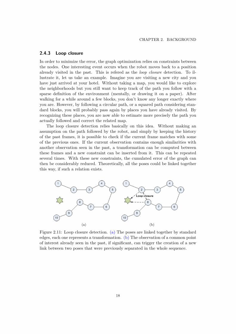
2.4.3 Loop closureIn order to minimize the error, the graph optimization relies on constraints betweenthe nodes. One interesting event occurs when the robot moves back to a positionalready visited in the past. This is refered as the loop closure detection. To il-lustrate it, let us take an example. Imagine you are visiting a new city and youhave just arrived at your hotel. Without taking a map, you would like to explorethe neighborhoods but you still want to keep track of the path you follow with asparse definition of the environment (mentally, or drawing it on a paper). Afterwalking for a while around a few blocks, you don’t know any longer exactly whereyou are. However, by following a circular path, or a squared path considering stan-dard blocks, you will probably pass again by places you have already visited. Byrecognizing these places, you are now able to estimate more precisely the path youactually followed and correct the related map.

The loop closure detection relies basically on this idea. Without making anassumption on the path followed by the robot, and simply by keeping the historyof the past frames, it is possible to check if the current frame matches with someof the previous ones. If the current observation contains enough similarities withanother observation seen in the past, a transformation can be computed betweenthese frames and a new constraint can be inserted from it. This can be repeatedseveral times. With these new constraints, the cumulated error of the graph canthen be considerably reduced. Theoretically, all the poses could be linked togetherthis way, if such a relation exists.

(a) (b)

Figure 2.11: Loop closure detection. (a) The poses are linked together by standardedges, each one represents a transformation. (b) The observation of a common pointof interest already seen in the past, if significant, can trigger the creation of a newlink between two poses that were previously separated in the whole sequence.

18

2.4. GENERAL CONCEPTS FOR SLAM

2.4.4 Graph optimizationThe detection of loop closures leads to new constraints that can be inserted intothe graph as new edges, linking the related poses. The optimization of the graphconsists in finding the optimal configuration of vertices to respect all the givenconstraints, as illustrated in figure 2.12.

Figure 2.12: Overview of the graph optimization procedure

19


2.5 SummaryThis chapter gives an overview of some of the main concepts used for SLAM andmore specifically VSLAM, defining the outlines of a possible approach to solve theproblem. The features allow to track some points of interest and can be used toevaluate a unitary move between a couple of frames. By combining them together,an estimation of the trajectory of the camera could be estimated. With the use ofa pose graph, and after detecting loop closures, the graph could be optimized inorder to reduce the global drift error. From the corrected camera poses, a map canthen be built.

While the performance is not the main issue of this work, it is still possible tomake a distinction between the operations that can be performed online (while therobot is moving) and the operations done offline (after a given sequence of moves).While the SLAM addresses both Localization and Mapping, the solution based onthe graph implies the detection of loop closures to give a correct result. Therefore,the dual problem of building the map and localizing the robot at the same time ismore likely to be done offline. This is one of the main constraint resulting of thisapproach. However, once the map is built, the single operation of localization couldbe done on the basis of the relevant features that have been used during the initialSLAM operation. This kind of approach could allow the robot to build a map as afirst step, only for this purpose. Once the map is built, the localization and furtheroperations could be done, but this mainly depends on the tasks the robot has tofulfill.

20

Chapter 3

Feature matching

In the context of this work, the goal is to track some keypoints precisely and toevaluate the motion of the camera from the keypoint coordinates. In this chapter,we present how the extraction of features is performed and how the keypoints arematched, in order to compute a rigid transformation between a couple of frames.

3.1 Feature extractionThe first question is the choice of the features, starting from those listed in ta-ble 2.1. As the performance is not an issue yet, we will rather consider the wellknown SIFT and SURF, for which many implementations exist, but also the morerecent NARF [22]. The BRIEF descriptor can then be introduced later if necessary,assuming the detector is already given. One important difference is that SIFT andSURF are computed from the RGB data in 2D, while the NARF keypoints arecomputed from the 3D point cloud, involving both RGB and depth data. Beforelooking at scale and rotation invariance, one important condition that can easily beverified is the stability of the keypoints if the camera does not move.

We first tested the NARF descriptor provided by the PCL. The keypoints showedto be unstable while the camera was not moving. These variations could be ex-plained by the noise of the depth data of the Kinect, affecting the NARF detector.A better tuning may give more stable results, but apparently this feature was ratherdesigned for range scans such as laser range finders or stereo cameras which aregenerally more accurate, or less sensible to noise than the Kinect sensor. For thisreason, we preferred to work with the 2D image, first using SIFT feature which iswidely used in the community and known to be robust. Here, we tested the librarydeveloped by Rob Hess [12]. In order to keep only features that are interesting forthe next steps of the processing, the features are removed if the depth data on thispoint is not available (occlusion) or if the depth data is outside a fixed range ofdepth distance. Here, a maximum range of 5 meters is used.

21

CHAPTER 3. FEATURE MATCHING

3.2 Comparison of SIFT and SURFAfter testing simple extractions and getting satisfying results with the SIFT feature,the same experiments were repeated using the SURF features. The implementationprovided in OpenCV1 was used. We noticed a considerable gain in performance fora similar number of features. Globally, for a scene requiring about 1000ms withSIFT, the extraction of the SURF feature takes about 250ms, meaning that thetime is reduced by a factor of 4 which is significant.

Both algorithms have various parameters that will result in more or less featuresat the cost of computational time. In particular, for SIFT it concerns the numberof scales k computed for each octave (see figure 2.2) and the variance σ of theGaussian. Here, the default values of the SIFT library [12] are used, which are alsothe standard values recommended by David Lowe (k = 3, σ = 1.6). Refer to themethod [16] for the description of these parameters. For SURF, another parameteris the threshold of the Hessian. Only features with Hessian larger than this valueare extracted.

In order to compare both methods, we first tried to find a configuration of pa-rameters giving similar number of features, using a dataset of 6474 frames describedin chapter 5 (see also the description of the hardware and software configuration).For an image of 640x480 pixels, the number of octaves set in the SIFT Library is6. By setting the same number of octaves at 6 and a Hessian threshold of 300 forSURF, we get a very close number of features. Then, we compare with the defaultsettings which implies a number of octaves of 3 and a Hessian threshold of 500. Theresults are summarized in the table 3.1.

Avg nb features Avg time Avg time by feature(in ms) (in ms)

SIFT 6 745 894 1.407SURF 6/300 711 345 0.582SURF 3/500 384 178 0.586

Table 3.1: Comparison of SIFT and SURF features, averaged for 6474 frames. Fora similar number of features, SURF is almost 3 times faster than SIFT. For halfnumber of features, there is a gain of factor 5.

1http://opencv.willowgarage.com/

22

http://opencv.willowgarage.com/

3.2. COMPARISON OF SIFT AND SURF

Figure 3.1: Comparison of SIFT and SURF – time for computing features. SURFis about 2.6 times faster than SIFT for a similar number of features. For differentSURF parameters, the time is linearly proportional to the number of features (x2faster for x2 less features).

Figure 3.2: Comparison of SIFT and SURF – average time by feature. SURF isfastest and it does not depend on the given parameters.

23


3.3 Initial Matching

Now that the features can be computed, it is possible to look for their matchingbetween a couple of frames. The initial matches can be found through a nearestneighbor search, using the Euclidean distance computed on the descriptors of thesefeatures. The SIFT Library [12] proposes an implementation of the Best-Bin-Searchdescribed by Lowe [16], based on kd-tree. For each feature in the target frame, thetwo nearest neighbors are searched in the source frame. If these neighbors are closeenough (with respect to a fixed threshold), then the result is considered to be valid.This initial search is done on the 2D features. To increase robustness, matches arerejected for those keypoints where the ratio of the nearest neighbor distance to thesecond nearest neighbor distance is greater than a given threshold, set to 0.5 here.After this, the depth information is used to keep the features that are close enoughto the camera, as the accuracy of the depth information is not considered reliableenough above a given range (around 5-6 meters).

Figure 3.3: Initial matching of SIFT features

24

3.4. ESTIMATION OF THE 3D TRANSFORMATION

3.4 Estimation of the 3D transformationFrom the matching pairs, it is possible to find a rigid transformation binding the twosets of points, i.e. the operation that projects each feature point of a source frameto the corresponding point in the target frame. In our case, this transformation is aperspective projection for 6 degrees of freedom, composed by a rotation matrix anda translation vector in 3 dimensions. This transformation can be written by usinga 4x4 matrix and homogeneous coordinates. We can then project a point P whereP = (x, y, z, 1)T simply by applying this transformation matrix to the point:

P ′ = Ttransformation P

The points defined by the initial matching pairs need to be converted in 3 di-mensions. For this, we need to define a proper coordinate system. To make thenext steps easier (graph optimization and scene reconstruction) and avoid furtherconversions, we keep the same coordinate system for all the work, defined as follows:

x : depth, positive forwardy : height, positive upwardsz : width, positive to the right

Figure 3.4: The two different coordinate systems, from the "screen" (as seen by thesensors RGB-D) to the 3D scene in the real world.

From the depth value (given in mm by OpenNI) and the screen coordinates(with RGB color and a resolution of 640x480 pixels), it is possible to compute thepoints coordinates in 3D. Let (u,v) be the point coordinates in pixels, we have then:

P (x, y, z)

x = depthy = −(v − 480/2) ∗ depth/focal_lengthz = (u− 640/2) ∗ depth/focal_length

25


Considering the initial matches, the next step is then to find a transformationmatrix, that gives a satisfying projection for most of these points. Ideally, we couldsimply compute a transformation by a least square method for all these points, eachmatching pair defining an equation. The minimum number of pairs required for thiswould be three, and the more points, the better defined the system would be. How-ever, because of the uncertainty due to the sensory noise and the feature matchingby itself, a single point which location is incorrectly estimated could lead to a sig-nificant error in the final transformation. Therefore, a better transformation can befound iteratively with the RANSAC method described in the background (2.3.1).In this context, we can precise the algorithm:

Algorithm 2 Find the 3D transformation with RANSACRequire: initial pairs of 3D points (origin, destination)bestTransform, bestInliers← ∅Define the number of iterations Nfor iteration = 1 to N dosamples← pickup randomly k pairs (origin, destination)Compute currentTransform from samplesinliers← ∅for all pairs of points doprojectedi ← projectPoint(origini, currentTransform)error ← computeDistance(projectedi − destinationi)if error < threshold theninliers← inliers+ pairi

end ifend forCount number of inliers and compute mean errorif currentTransform is valid thenRecompute currentTransform from inliersif currentTransform better than bestTransform thenbestTransform← currentTransformbestInliers← inliers

end ifend if

end forreturn bestTransform, bestInliers

As mentioned in the section 2.3.1, it is possible to estimate the optimal valueof N to satisfy a target probability of inliers ratio. In this work we use a fixedvalue given by parameter of N=20. It may be tuned more accurately with a deeperstudy of the RANSAC procedure. Generally, if the quantity of features is high, theprobability of having an outlier is lower at this step, as most of the mismatches havealready been excluded by the initial matching.

26

3.5. ANALYSIS

To compute a transformation (an hypothesis), only the k samples from theinitial matches are used each time. The 3D points are converted to homogeneouscoordinates and the transformation is given by solving the corresponding equationfrom the known constraints which are defined by the chosen points. This is can bedone through a Singular Value Decomposition (SVD) of the covariance data. To dothis, we use the minimal number of points to solve this equation, k=3.

To evaluate a transformation, each sample taken from the initial matches (source)is then projected according to this transformation. A 3D vector is computed fromthe difference between the projected point and the real point taken from the match-ing point (destination). The error is the norm of this vector.

3.5 AnalysisSome preliminary experiments were conducted to determine how to find a satisfy-ing transformation between a couple of frames. In this context, the unitary movebetween two frames should be generally small if we consider a limited motion ofthe camera (by amplitude and speed). The larger the move, the more difficult itbecomes. To do this, a program was written to perform the feature extraction withthe initial matching and the RANSAC iterations, taking a couple of RGB-D framesas an input.

(a) Initial matching (b) After RANSAC

Figure 3.5: Matching of SIFT features: (a) initial matching from KNN search(b) after running RANSAC. Some of the initial matches drawn in diagonal (green)in the left figure are excluded and become outliers (red) after RANSAC.

27


Characterizing a transformation There are at least 3 parameters:

• Mean error: the norm of the error vector. Lower is better.

• Number of inliers: the absolute number of inliers. Higher is better.

• Ratio of inliers: the relative number of inliers with respect to the initialmatches. Higher is better.

The main difficulty is to find the best balance among these 3 values, by puttingsome thresholds. Setting too high constraints would lead to the impossibility to finda transformation satisfying all the criteria. This is true especially when there are notenough features detected. Setting too low constraints helps to find a transformationeven when there are less features or the measurements are noisy, but the resultingtransformation will be less precise. The main risk here is to set too loose constraintsso the inliers would include some mismatches. If the criteria are too permissive,this would result in an invalid model, leading to incorrect associations, as shown infigure 3.6.

Figure 3.6: Example of an incorrect model. The matches are incorrect, as the scenesand objects are completely different. But the green lines are considered to be inliers,due to the similarity of the dark lines. Here, the threshold defining the minimumratio of inliers with respect to the initial matches is too low.

28

3.5. ANALYSIS

Quality of a transformation A good transformation should be valid for most ofthe given points. But this definition is not enough, as only considering the numberof inliers is not necessarily the best choice. Another criterion could be the spreadof the inliers. If many inliers are concentrated on a small area, they don’t givemuch added value with respect to the global transformation of the scene. A bettertransformation may be found including more distant points, if their projection erroris just slightly above the threshold. This could be measured by computing the meanposition of the inliers and, from this, the standard deviation, or more simply thevariance of the inliers.

Let N be the number of inliers and pi be the i-th inlier vector. We can thencompute the mean vector µ and the variance σ2 with their standard definitions:

µ = 1N

N∑i=1

pi σ2 = 1N

N∑i=1

(pi − µ)2

Figure 3.7: Sequence showing different distributions of the inliers. Note how theinliers are grouped in the case shown in the middle.

inliers/matches ratio σ2(2D) σ2(3D)93/114 81% 0.345409 1.223234/119 28% 0.0203726 0.051973791/135 67% 0.476902 1.42809

Table 3.2: Ratio of inliers shown in figure 3.7, variance of the keypoints in 2D(without depth information) and 3D.

29


The variance may be used to detect these situations. Instead of using the ratioof inliers as the criterion to measure the quality of the model, the variance couldbe used, not only as an evaluation of the goodness ("score") but also as a criterionfor the selection of the k elements of each sample. For example, the initial elementswould have above a minimal distance from the mean, set by a threshold. Thisconcept could not be developed in the given time, but it could be studied in futureworks.

3.6 SummaryIn this chapter, we presented a method to compute a rigid transformation froma couple of frames given their RGB-D data. This transformation represents themotion of the camera between two consecutive frames, for 6 degrees of freedom.This was done through the following steps:

1. first, the SIFT/SURF features are extracted from each RGB frame (using only2D);

2. an initial matching is performed with the use of a kd-tree, and the depthinformation is integrated to compute the feature positions in 3D;

3. from this set of pairs of features, a transformation is computed by running aRANSAC algorithm.

The figure 3.8 illustrates how the RGB and depth input data can be used to com-pute the sequence of 3D transformations, and subsequently, the initial estimationof the poses.

Figure 3.8: Processing of the RGB-D data

30

Chapter 4

Building a map

In the previous chapter, we saw how to determine a rigid transformation between acouple of frames. From each single transformation, an estimation of the poses of thecamera can be computed. Now we can combine them to proceed with a sequence offrames. Each pose is then inserted into the graph by converting its representationfrom the camera matrix into a graph node. From the loop closures, new constraintscan be inserted in the graph. The graph can then be optimized to minimize anerror function, and the poses are updated according to the new vertices given bythe graph after optimization, reducing the global drift.

4.1 Estimating the poses

Knowing the initial pose, the first step is to determine an estimation of any poseafter a succession of transformations. Considering a finite sequence of frames[frame0; frameN ], let Pk be the pose at rank k ∈ [0;N ]. For 6DOF, composedby 3 axis of rotation and translation, it can be represented by a 4x4 matrix withhomogeneous coordinates, where R is a 3x3 rotation matrix and t a translationvector:

Pk =

Rtxtytz

0 0 0 1

For i > 0, we have the transformation T ii−1 that binds the position Pi−1 to

the position Pi. Each transformation T can also be represented by a similar 4x4matrix. If P0 determines the initial position, we can then compute the position Piby combining all the transformations like:

Pk =1∏i=k

T ii−1 P0 (4.1)

31

CHAPTER 4. BUILDING A MAP

As the matrix product is not commutative, it is essential to follow the correctorder when multiplying the matrices. For example, for the pose P3 we have:

P3 = T 32 T

21 T

10 P0

Generally, the initial position is defined by the initial orientation of the camerafor each axis, stored in the initial rotation matrix R0, and the initial translationvector t0 = (x0, y0, z0)T , as follows:

P0 =

R0

x0y0z0

0 0 0 1

As an arbitrary choice, we can define the initial position to be at the origin of

the coordinate system, which is given by the identity matrix I4.

P0 = I4 =

1 0 0 00 1 0 00 0 1 00 0 0 1

4.2 Initializing the graphThe equation 4.1 gives an estimation of the pose that can be inserted into the g2ograph. However, a sequence of video frames can contain an important number ofsimilar poses, especially if the robot slows down, or even stops. Inserting a node foreach transformation would lead to many redundant poses. It makes good sense toinsert a new pose only after a significant change from a given pose. To distinguishthem among all the others that can potentially be inserted in the graph, these posesare called the keyposes.

A simple solution is to define a keypose only after having achieved a move, witha given amplitude defined by a threshold. By cumulating the unitary moves betweeneach couple of frames in the sequence, the creation of a new key pose is triggeredonce a given distance in translation or a given angle in rotation has been reached,with respect to the last key pose. The thresholds are set by parameters, here 0.1mfor the distance and 15°for the rotation (both values consider the variations on the3 axis cumulated together). Another solution would be to compare the points ofinterests between the frames and trigger the creation of a new keypose when thenumber of points in common falls below a given threshold, but it is not given thatthe absolute number of points is representative enough to describe the amplitudeof the move.

For each keypose, a node is inserted in the graph with an edge linking the newkeypose with the previous one. A standard edge represents the rigid transformationbetween the two keyposes. Between each keypose, they may be a more than a coupleof frames. To compute the corresponding transformation, the resulting matrix isfound by multiplying all the intermediate matrices for each couple of frames.

32

4.3. LOOP CLOSURES

4.3 Loop closures

The detection of loop closures can be translated into additional constraints in thegraph, as illustrated in figure 2.12. Each time a loop closure is triggered betweentwo keyposes, a new edge is inserted into the graph. Here, the detection of the loopclosure is done by computing a transformation between the two frames, as describedin section 3.4. If there are enough inliers to make the transformation valid, a loopclosure can be inserted.

Following the order of the sequence, the detection of a loop closure can be doneby comparing the most recent frames with previous ones. The naive approach wouldbe to check for the whole set of frames, comparing the current frame with all theprevious frames. However, this can be highly time consuming, as the time necessaryfor the current frame would grow fast. For example, for 4 frames, there would be 6checks to perform by looking in the past (respectively 1,2,3 checks for each frame).For N frames, there would be (N − 1) ∗ N/2 checks to perform. Clearly, this canbecome an issue if the check is not fast enough. First, it can be optimized by storingthe past features into a memory buffer. A preliminary check exclusively done onthe RGB data, for example with color histograms, could also be used to discardmost of the negative candidates. Then, a more accurate verification would involvethe features for the remaining candidates.

In this work, for reason of performance, it was necessary to reduce the list ofcandidates to check. Without making any assumption on the past frames, the firstidea is to define a sliding window with a fixed size of k frames in the past. The loopclosure is of interest when it closes a loop with frames that are sufficiently distant inthe temporal sequence, as the goal is to reduce the drift over time. For this reason,from a given frame, it is more appropriate to check with older frames in the pastrather than most recent ones. By defining a number of excluded frames and thesize of the sliding window, an efficient method can be implemented.

(a)

(b)

Figure 4.1: Illustration of a sliding window of 5 frames, where the last 3 frames areignored. (a) For the current frame n.9, the frames 1-5 are checked. (b) For the nextframe n.10, the window slides one step forward. The frames 2-6 are checked.

33


However, these parameters are hard to define without a prior knowledge ofthe followed path. To extend the search, but still limiting the number of checks,these frames could be selected randomly in a much larger window, first assuming aconstant probability density function. But the goal is to select the past frames thatare more likely to match with the current frame, giving a higher priority to the oldestframes. This could be done defining a probability density function with a higherprobability for the oldest frames. This probability could also be defined consideringthe knowledge of the context, in terms of features, or in terms of estimated position,preselecting the candidates with the highest likelihood.

Here, we limited the search by using a candidate list of N frames, ignoring themost recent frames (the size can be set by a parameter), and a probability densityfunction giving priority to the oldest frames. To select the N candidate frames, thefunction giving the probability to select a candidate can be defined by p(i) = i/S,where S = (N + 1) ∗N/2. For a sliding window of 3 frames, the first frame wouldhave the probability 3/6, the second 2/6 and the third 1/6. These values can thenbe normalized for a total probability of 1.

To improve the quality of the loop closure detection, once a candidate frame isfound, the check is extended to its neighbors, looking for a better transformation.The ratio of inliers is used to measure the quality of the transformations and tocompare them. We consider only a forward search, meaning that the followingneighbors will be checked, as illustrated in figure 4.2.

Figure 4.2: Loop closure with forward search for the pose Pk. First, a valid trans-formation is found with candidate C1. The check is then performed with the nextframe C2, giving a better transformation. The search continues forward, and foundsa better transformation with C3. Finally, the quality of the transformation with C4is lower, so the process stops. The loop closure is inserted between Pk and C3.

34

4.4. OPTIMIZING THE GRAPH

4.4 Optimizing the graphOnce the graph has been initialized with the poses and the constraints from theloop closures, it can be optimized. Various methods are available in g2o, bothfor the optimization process and the solving problem. The method used here isLevenberg-Marquardt with a linear Cholmod solver. The optimization is done witha predefined number of steps. Once the graph has been optimized, the vertices arecorrected and the new estimations of the camera poses can be extracted. Similarlyto the insertion, the inverse operation is done to convert the information from thegraph vertices to 4x4 matrices.

(a) initial graph

(b) optimized graph

Figure 4.3: Visualization of the graph with the g2oviewer, (a) non optimized, (b) af-ter 10 iterations, for a map of 4 rooms (experiments are described in chapter 5).

35


4.5 Scene reconstructionFinally, once the camera poses are determined with a good belief, the reconstructionof the scene can be performed. For each frame, a 3D point cloud can be generatedfrom the RGB and depth data, providing the colour information for each point.However, in order to reconstruct the whole scene, they have to be combined togetherfrom a unique point of view. This process is called the point cloud registration. Oncethe camera positions are known, each point cloud is transformed by projecting all itspoints according to the corresponding camera position, given by the equation 4.1.This is done relatively to the first pose, which is predefined. The transformed pointclouds are then concatenated together to build the scene.

This method is simple, the major issues are that it leads to duplicate points,and it does not take variances of illumination into account. Some considerationsabout memory are described in the experiments, in section 5.5. However, the pointcloud is not necessarily the best representation of the scene. For many applications,it would be preferable to define some dense surfaces, such as the surfels presentedin [17] and used in the work of Henry [11], but this would require further study andprocessing and it is out of the scope of this work.

4.6 SummaryIn this chapter, we presented how the poses can be estimated, first by cumulatingeach transformation between a couple of frames. Through the use of a pose graphand the loop closures, their positions can be corrected over time. Finally, the mapcan be built from a scene reconstruction, by registration of the point clouds withthe given positions of the cameras.

36

Chapter 5

Experiments

After studying the feature extraction and matching, the graph optimization andthe reconstruction, some experiments could be done. A software was developed,which goal is to acquire data from the Kinect, compute the 6DOF camera posesrepresenting the trajectory and orientation of the robot, and produce a 3D map.The following sections describes how the input data was acquired, and how theoutput is generated. The next sections present the maps obtained from differentdatasets, first from KTH, for different sizes (1 room, 2 and 4 rooms with corridor).The last section shows the results obtained with data from other universities.

5.1 System overviewThe program can perform the following tasks:

• acquires a stream of RGB-D data from the Kinect;

• performs extraction and matching of SIFT/SURF features;

• computes the relative transformations with RANSAC;

• computes the initial poses and translates them into g2o nodes and edges;

• detects the loop closures and inserts the corresponding edges into the graph;

• optimizes the graph with g2o and extracts the updated camera poses;

• reconstructs the global scene by generating a point cloud datafile (*.pcd).

The sequence of actions, which have been described in the previous chapters,can be summarized in the figure 5.1. Note: the use of RGB and depth data is moredetailed in figure 3.8.

37

CHAPTER 5. EXPERIMENTS

Figure 5.1: Overview of the system

In order to repeat the experiments with different parameters, the RGB-D streamis saved and the program is able to replay a given sequence from a list of files. Twotypes of experiments were conducted:

• on the fly, by moving the Kinect sensor by hand, with a feedback in real time;

• offline, by recording a data stream with a mobile robot, and processing itafterwards.

In the first case, the program performs the feature extraction and computes thetransformations in real time. When the motion is too fast, or when the numberof features is too low, the synchronization can be lost if no valid transformation isfound between the last two frames. The sequence is then suspended and a messageis displayed, so the user can move the camera back and lock again with the lastvalid frame, to resume the sequence. The detection of the loop closures, the graphoptimization, and the reconstruction are done in a next step. Similarly, all theprocessing could have been done on the robot as well, but this would require furtherinstallations, and here the goal was to generate a set of reference data, as describedin the section 5.2.

The main program was executed on a PC equiped with an Intel Core™ i3–540 CPU(3.06 GHz, 4MB cache) and 3GB of RAM, running on Linux Ubuntu 10.04 (ker-nel 2.6.35.7). When the acquisition and matching are done on the fly, the system isable to process about 3-4 frames per second using SURF, which is already enoughto let the user walk slowly in a room, with a real time feedback. Most of the timeis spent for the feature extraction (100-200ms). Some possible improvements aregiven in the final chapter with the conclusions.

38

5.2. DATA ACQUISITION

5.2 Data acquisition

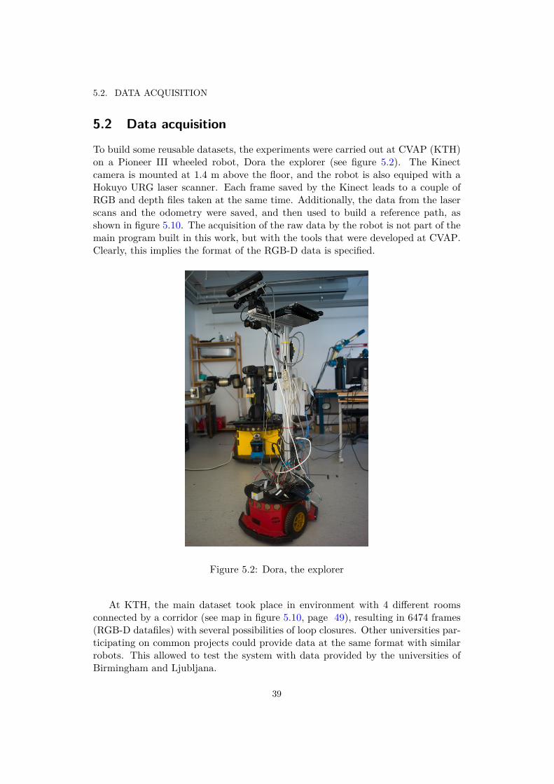
To build some reusable datasets, the experiments were carried out at CVAP (KTH)on a Pioneer III wheeled robot, Dora the explorer (see figure 5.2). The Kinectcamera is mounted at 1.4 m above the floor, and the robot is also equiped with aHokuyo URG laser scanner. Each frame saved by the Kinect leads to a couple ofRGB and depth files taken at the same time. Additionally, the data from the laserscans and the odometry were saved, and then used to build a reference path, asshown in figure 5.10. The acquisition of the raw data by the robot is not part of themain program built in this work, but with the tools that were developed at CVAP.Clearly, this implies the format of the RGB-D data is specified.

Figure 5.2: Dora, the explorer

At KTH, the main dataset took place in environment with 4 different roomsconnected by a corridor (see map in figure 5.10, page 49), resulting in 6474 frames(RGB-D datafiles) with several possibilities of loop closures. Other universities par-ticipating on common projects could provide data at the same format with similarrobots. This allowed to test the system with data provided by the universities ofBirmingham and Ljubljana.

39


University Dataset Rooms FramesKTH 7th floor 1 3082KTH 7th floor 2 2697KTH 7th floor 4 6474Birmingham Lab3 1 1342Birmingham Robotic Lab 1 2878Ljubljana Office1 1 2088Ljubljana Office2and3 2 5687

Table 5.1: Description of the different datasets. Note the KTH set of 1 roomcontains more frames than for 2 rooms, due to the robot moving at a slower speed.

5.3 Software implementationThe code is available as an open source project1. It is released with a LGPL v3license. The number of dependencies has been limited to a reasonable set of open-source libraries. Unlike the RGBD-6D-SLAM project [5], it is not based on ROSframework, and PCL is mainly used for the reconstruction at the final step. Themain dependencies are the following:

• g2o: the graph optimization

• OpenNI: to acquire the Kinect data

• OpenCV: open source library used to visualize the intermediate results withbitmaps (frame matching) and compute the SURF features

• SIFT Library by Rob Hess [12]: for the SIFT extraction and initial matching

• Eigen3: for the geometric support with transformations and matrices

• Point Cloud Libary [21], standalone distribution (cminpack, Flann, Eigen3,OpenNI): for the transformations and the export to point cloud datafiles

• Boost: support library, used here to access the filesystem

1http://code.google.com/p/kth-rgbd/

40

http://code.google.com/p/kth-rgbd/

5.4. USER INTERFACE

5.4 User interfaceTo use the program in real time, a simple graphical user interface was developed.The main window displays two frames with their features. The upper frame is thecurrent frame, and the lower frame is the last valid frame. If the sequence is out ofsynchronization, meaning that no valid transformation between the last two frames,this layout allows the user to move back by comparing visually the current framewith the last valid one. Then, the sequence is resumed automatically as soon asthere is a valid transformation. The quality of the transformation is also displayed,that corresponds to the ratio of inliers.

Figure 5.3: user interface, displaying the current and last frames with their features

41


5.5 Data outputAs a result, the program exports the positions of the cameras, and the map repre-sented by a point cloud (PCL). For reasons of performance, it is necessary to controlthe memory storage by limitating the size of the final point cloud. Theoretically,each point cloud can be composed of 640 × 480 = 307, 200 points. Practically, theeffective number of points is lower, as the depth information is not available foreach point (due mainly to the range limit and to the occlusions considering thedifference of point of view between the IR and RGB sensors). A standard pointcloud is composed of about 200,000 points. For each pixel, 24 bits are used for thepositions (x,y,z) and 24 bits for the colors R,G,B (3× 8 bits), padded to 8 bytes foralignment in memory. Therefore, a colored cloud point occupies around 200k × 8= 1.6MB in memory. For a scope of visualization, it is reasonable to reduce theamount of information. Each point cloud is first subsampled simply by removingpoints taken randomly with a given probability (according to a fixed ratio, set as aparameter depending on the global size of the scene).

Generally, only one output file is produced but this can still lead to a big filein case of a large map. In this case, the total number of points can be importantand a too high rate of subsampling would result in a low quality map. By setting athreshold for the size of the final point cloud file, it can be split in several subfileseach time the threshold is reached during the reconstruction of the global map. Theresult is then divided in different files. This allows to keep a low subsampling rate,and still to visualize a portion of the global scene with a good definition. For thevisualization of the point clouds, the standard viewer provided in PCL is used.

42

5.6. MAP AT CVAP – ONE ROOM

5.6 Map at CVAP – one room

This map is built from a sequence containing one room (see table 5.1), the graph isoptimized with one loop closure, which is triggered after having gone through theroom and back, close to the initial position.

(a) from initial graph

(b) from optimized graph

Figure 5.4: Map at CVAP with 1 room – (a) Without graph optimization. (b) Withloop closure. Note how the corner of the table and the chair appears to be doubledin the top figure, and how it is corrected in the bottom figure.

43


(a) from initial graph

(b) from optimized graph

Figure 5.5: Map with 1 room, details of the chair – (a) Without graph optimization.(b) With loop closure. The reduction of the drift is clearly noticeable.

44

5.7. MAP AT CVAP – TWO ROOMS AND CORRIDOR

5.7 Map at CVAP – two rooms and corridor

This map is built from a sequence containing two rooms separated by a corridor(see table 5.1). The graph is optimized with two loop closures, the first one withan internal loop in the living room, and the other one at the end of the sequence,after coming back in the first room close to the initial position.

Figure 5.6: Map with 2 rooms, optimized with two loop closures. The rooms areclearly displayed and correctly oriented. The main issue concerns the dividing wallin the corridor.

45


5.8 Map at CVAP – four rooms and corridorThis map is built from a sequence containing four rooms separated by a corridor(see table 5.1), first without graph optimization.

Figure 5.7: Map with 4 rooms and corridor, not optimized. The main issue thatcan be noticed at this scale is the relative orientation of the first room (first figure,bottom right), which looks misaligned, and its desk appears to be doubled.

46

5.8. MAP AT CVAP – FOUR ROOMS AND CORRIDOR

For the following map, the graph is optimized with four loop closures, triggeredwith a loop in three rooms room and the other one at the end of the sequence, aftercoming back in the first room close to the initial position.

Figure 5.8: Map with 4 rooms and corridor, optimized with several loop closures.The alignment of the first room looks better (first figure, bottom right), but theliving room (bottom center) shows some misaligned frames. This is a trade-off withrespect to the global error.

47


(a)

(b)

(c)

Figure 5.9: Estimation of the poses – (a) From standard odometry, raw data. Notethe drift, as the start and end points should be pretty close. (b) With this system,initial graph. (c) With the optimized graph. There is a slight variation.

48

5.8. MAP AT CVAP – FOUR ROOMS AND CORRIDOR

To analyze the quality of the localization, we compared the resulting path withone close to the ground truth, generated by a SLAM system developed at CVAP,based on EKF using the laser scan data [7].

(a)

(b)

Figure 5.10: Trajectory overlayed on the reference map of the 7th floor, using (a)SIFT features. (b) SURF features. In both cases, the drift is noticeable, but theresults are relatively close. The total distance gives an indication of the accuracy.

49


Figure 5.11: Analysis of the vertical drift. The Y-coordinates have been shifted tothe origin for the starting position. Considering the camera is fixed on a support,the value should stay close to zero. This issue needs to be further investigated.

50

5.9. MAP FROM OTHER UNIVERSITIES

5.9 Map from other universitiesFor this map, the Lab3 dataset provided by the University of Birmingham was used.No particular issues were encountered.

Figure 5.12: Birmingham Lab3

51


For this map, the Robotic Lab dataset provided by the University of Birminghamwas used. An issue was raised due to the people moving during the passing of therobot, leading to some inaccuracies in the transformations. The system is not ableto handle such situations, affecting the feature matching, and therefore the overallquality of the map.

Figure 5.13: Birmingham Robotic Lab

52

5.9. MAP FROM OTHER UNIVERSITIES

For this map, the Office1 dataset provided by the University of Ljubljana wasused. It could only be processed partially, the sequence was interrupted for a lackof features. This is one intrinsic limitation of the method presented in this work.

(a)

(b)

Figure 5.14: Ljubljana office1 – (a) Map without closure loop. (b) Not enoughfeatures could be extracted at this point. This occurs typically when flat surfacesare predominant in the scene.

53


For this map, the Office2and3 dataset provided by the University of Ljubljanawas used. As for the previous dataset, it could only be processed partially, thesequence was interrupted for a lack of features.

Figure 5.15: Ljubljana office2 – map without closure loop

5.10 SummaryThese experiments show that 3D maps can be built with this system and illustratethe interest of the loop closure to get a good correction. Though the results aresatisfying for small maps, there can still be a noticeable drift as the size of the mapgrows. Here, some misalignments can be perceived with 4 rooms. The most obviouslimitations were also encountered, showing that the process can be interrupted assoon as there are not enough visual features to detect a valid transformation, andhow moving elements can alter the final result.

54

Chapter 6

Conclusions and Future Works

With this work, we could have a good insight into the general problem of SLAM, andmore specifically of VSLAM with feature extraction and matching. The approachcan be described by the following steps:

1. Feature extraction: SIFT/SURF extraction in 2D, preselection with depth;

2. Feature matching: nearest neighbors on the feature space, using kd-trees;

3. Transformation: computed with RANSAC on the 3D keypoints;

4. Graph optimization: based on the g2o framework, a better graph can becomputed with new constraints by detecting loop closures;

5. Scene reconstruction: registration of the points clouds accordingly to the es-timation of the keyposes, and concatenate them to build the global map.

Given this, it is now possible to imagine some improvements of the current work,both in terms of quality of the results and overall performance.

6.1 Quality improvements• Finding a better transformation: the RANSAC method returns a rigid trans-

formation that is not necessarily the best. The parameters may be tuned in amore efficient way to give more accurate results, or defined with a variant likeMLESAC [26]. The tuning also concerns the initial matching done with theSIFT/SURF features. The ICP [27] method should give a refined solution.The output of the RANSAC loop could be used as an initial guess for ICP.

• Graph optimization: it could be improved by formulating more accurately theoptimization problem and refining the minimization method (possibly with g2oby deriving new classes and defining appropriate error functions), and alsoby exploiting the possibilities of modularity, for example with hierarchicallevels corresponding to different scales for bigger maps. New criteria could

55

CHAPTER 6. CONCLUSIONS AND FUTURE WORKS

be defined for loop closures, by introducing some knowledge about the pastframes (features or estimated position more likely to give a loop closure withthe current frame) or by matching only a portion of scene that does notnecessarily give a valid transformation in the current system.

• Additional sensors: in this work, the only sensor used was the Kinect providingRGB-D data. One possibility would be to use others sensors and combinethem to get a better result in a multi-modal or hybrid system, especiallywhen the transformations computed by the method presented in this workare less reliable.

6.2 Performance improvementsCurrently, most of the time is passed on the feature extraction. Here are a fewalternatives :

• GPU implementation: a feature extraction optimized for the hardware ofthe graphic cards would dramatically lower the computational time to enablereal-time applications. Various GPU implementations exist for both SIFT andSURF. In addition, some solutions take advantage of the parallel computingon specific platforms, such as CUDA™ for the NVIDIA graphic cards. Thefeatures extraction could then be performed in 15-20ms [2].

• BRIEF: combined with a keypoint detector such as SURF or SIFT, the BRIEFdescriptors [3] could give an interesting alternative, being more efficient tocompute. However, this would imply to rewrite the matching code, by doingbinary string comparison. See also the PhD thesis of Calonder [4].

• ICP: though the standard algorithm could increase the computational time,some efficient variations exist [20].

6.3 Other approachWith the KinectFusion project, Microsoft Research presents a solution performingreconstruction without any feature, though it achieves real-time performance asdemonstrated1 at SIGGRAPH 2011. The camera tracking is based on a GPU im-plementation of ICP on the point clouds generated from the depth data. The relatedpapers [13] [19] describe how an accurate dense reconstruction can be performedin real-time, which sounds promising in the future for many applications related tocomputer vision, not only mapping but also segmentation and object recognition.A new version of the Kinect camera working at shorter range will also extend thepossibilites.

1KinectFusion: http://www.youtube.com/watch?v=quGhaggn3cQ (last access: Jan 2012)

56

http://www.youtube.com/watch?v=quGhaggn3cQ

Acronyms

BRIEF Binary Robust Independent Elementary Feature. 6, 13, 21, 56

CVAP Computer Vision and Active Perception Lab. 2, 39, 49

DOF Degrees-of-Freedom. 3, 31, 37

DoG Difference-of-Gaussian. 7, 8

EKF Extended Kalman Filtering. 2, 16, 49

HoG histogram of local oriented gradients. 8

ICP Iterative Closest Point. 15, 55, 56

NARF Normal Aligned Radial Feature. 6, 12, 21

PCL Point Cloud Library. 12, 21, 40, 42

RANSAC RANdom SAmple Consensus. 10, 13, 15, 26, 30, 37, 55

ROS Robot Operating System. 12, 40

SIFT Scalar Invariant Feature Transform. 6–8, 10, 13, 21, 22, 30, 40, 55, 56

SLAM Simultaneous Localization And Mapping. 1, 2, 16, 17, 20, 49, 55

SURF Speeded Up Robust Feature. 6, 10, 13, 21, 22, 30, 38, 40, 55, 56

SVD Singular Value Decomposition. 27

VSLAM Visual Simultaneous Localization And Mapping. 1, 3, 16, 20, 55

57

References

[1] Herbert Bay, Andreas Ess, Tinne Tuytelaars, and Luc Van Gool. Speeded-UpRobust Features (SURF). Comput. Vis. Image Underst., 110:346–359, June2008.

[2] M. Björkman. A CUDA implementation of SIFT, Computer Vision and ActivePerception Lab. http://www.csc.kth.se/~celle/. (last access: Jan 2012).

[3] M. Calonder, V. Lepetit, C. Strecha, and P. Fua. BRIEF: Binary Robust Inde-pendent Elementary Features. In European Conference on Computer Vision,September 2010.

[4] Michael Calonder. Robust, High-Speed Interest Point Matching for Real-TimeApplications (PhD Thesis), 2010.

[5] Nikolas Engelhard, Felix Endres, Jürgen Hess, Jürgen Sturm, and WolframBurgard. Real-time 3D visual SLAM with a hand-held RGB-D camera. InProc. of the RGB-D Workshop on 3D Perception in Robotics at the EuropeanRobotics Forum, Västerås, Sweden, April 2011.

[6] Martin A. Fischler and Robert C. Bolles. Random Sample Consensus: AParadigm for Model Fitting with Applications to Image Analysis and Auto-mated Cartography. Commun. ACM, 24(6):381–395, 1981.

[7] J. Folkesson, P. Jensfelt, and H.I. Christensen. The M-Space Feature Repre-sentation for SLAM. Robotics, IEEE Transactions on, 23(5):1024 –1035, oct.2007.

[8] G. Grisetti, R. Kümmerle, C. Stachniss, U. Frese, and C. Hertzberg. Hierarchi-cal optimization on manifolds for online 2D and 3D mapping. In Proc. of theIEEE Intl. Conf. on Robotics and Automation (ICRA), Anchorage, AK, USA,2010.

[9] G. Grisetti, C. Stachniss, S. Grzonka, and W. Burgard. A Tree Parameter-ization for Efficiently Computing Maximum Likelihood Maps using GradientDescent. Atlanta, GA (USA), 2007.

[10] C. Harris and M. Stephens. A Combined Corner and Edge Detector. In Pro-ceedings of the 4th Alvey Vision Conference, pages 147–151, 1988.

59

http://www.csc.kth.se/~celle/

REFERENCES

[11] Peter Henry, Michael Krainin, Evan Herbst, Xiaofeng Ren, and Dieter Fox.RGB-D Mapping: Using Depth Cameras for Dense 3D Modeling of IndoorEnvironments, Delhi, India, 2010.

[12] Rob Hess. An Open-Source SIFT Library. http://blogs.oregonstate.edu/hess/code/sift/. (last access: Jan 2012).

[13] Shahram Izadi, Richard A. Newcombe, David Kim, Otmar Hilliges, DavidMolyneaux, Steve Hodges, Pushmeet Kohli, Jamie Shotton, Andrew J. Davi-son, and Andrew Fitzgibbon. KinectFusion: real-time dynamic 3D surfacereconstruction and interaction. In ACM SIGGRAPH 2011 Talks, SIGGRAPH’11, pages 23:1–23:1, New York, NY, USA, 2011. ACM.

[14] Kurt Konolige and Motilal Agrawal. FrameSLAM: From Bundle Adjustment toReal-Time Visual Mapping. IEEE Transactions on Robotics, 24(5):1066–1077,2008.

[15] Tony Lindeberg. Scale-Space Theory in Computer Vision. Kluwer AcademicPublishers, Norwell, MA, USA, 1994.

[16] David G. Lowe. Distinctive Image Features from Scale-Invariant Keypoints.International Journal of Computer Vision, 60(2):91–110, November 2004.

[17] Hanspeter Pfister, Matthias Zwicker, Jeroen van Baar, and Markus H. Gross.Surfels: surface elements as rendering primitives. In SIGGRAPH, pages 335–342, 2000.

[18] Rainer Kuemmerle, Giorgio Grisetti, Hauke Strasdat, Kurt Konolige, and Wol-fram Burgard. g2o: A General Framework for Graph Optimization. IEEEInternational Conference on Robotics and Automation (ICRA), 2011.

[19] Richard Newcombe, Shahram Izadi, Otmar Hilliges, David Molyneaux, DavidKim, Andrew Davison, Pushmeet Kohli, Jamie Shotton, Steve Hodges, AndrewFitzgibbon. KinectFusion: Real-Time Dense Surface Mapping and Tracking.In 10th IEEE International Symposium on Mixed and Augmented Reality (Pro-ceedings of ISMAR 2011), October 2011.

[20] S. Rusinkiewicz and M. Levoy. Efficient Variants of the ICP Algorithm. 3DDigital Imaging and Modeling, International Conference on, 0:145, 2001.

[21] Radu Bogdan Rusu and Steve Cousins. 3D is here: Point Cloud Library(PCL). In IEEE International Conference on Robotics and Automation(ICRA), Shanghai, China, May 9-13 2011.

[22] B. Steder, R. B. Rusu, K. Konolige, and W. Burgard. NARF: 3D RangeImage Features for Object Recognition. In Workshop on Defining and SolvingRealistic Perception Problems in Personal Robotics at the IEEE/RSJ Int. Conf.on Intelligent Robots and Systems (IROS), Taipei, Taiwan, 2010.

60

http://blogs.oregonstate.edu/hess/code/sift/

http://blogs.oregonstate.edu/hess/code/sift/

REFERENCES

[23] Hauke Strasdat, J. M. M. Montiel, and Andrew J. Davison. Scale Drift-AwareLarge Scale Monocular SLAM. In Matsuoka, Yoky and Durrant-Whyte, HughF. and Neira, José, editor, Robotics: Science and Systems. The MIT Press,2010.

[24] S. Thrun and M. Montemerlo. The GraphSLAM Algorithm With Applicationsto Large-Scale Mapping of Urban Structures. International Journal on RoboticsResearch, 25(5/6):403–430, 2005.

[25] Sebastian Thrun, Wolfram Burgard, and Dieter Fox. Probabilistic Robotics(Intelligent Robotics and Autonomous Agents series). Intelligent robotics andautonomous agents. The MIT Press, August 2005.

[26] Philip H. S. Torr and Andrew Zisserman. MLESAC: A New Robust Estimatorwith Application to Estimating Image Geometry. Computer Vision and ImageUnderstanding, 78(1):138–156, 2000.

[27] Zhengyou ZHANG. Iterative Point Matching for Registration of Free-formCurves, 1992.

61

building a 3d map from rgb-d sensors

Documents