Full Terms & Conditions of access and use can be found athttp://www.tandfonline.com/action/journalInformation?journalCode=uhvc21

Download by: [Xiwang Li] Date: 07 July 2016, At: 06:41

Science and Technology for the Built Environment

ISSN: 2374-4731 (Print) 2374-474X (Online) Journal homepage: http://www.tandfonline.com/loi/uhvc21

Commercial building cooling energy forecastingusing proactive system identification: A wholebuilding experiment study

Xiwang Li, Jin Wen, Ran Liu & Xiaohui Zhou

To cite this article: Xiwang Li, Jin Wen, Ran Liu & Xiaohui Zhou (2016): Commercialbuilding cooling energy forecasting using proactive system identification: A wholebuilding experiment study, Science and Technology for the Built Environment, DOI:10.1080/23744731.2016.1188654

To link to this article: http://dx.doi.org/10.1080/23744731.2016.1188654

Published online: 06 Jul 2016.

Submit your article to this journal

View related articles

View Crossmark data

Science and Technology for the Built Environment (2016) 0, 1–18Copyright C© 2016 ASHRAE.ISSN: 2374-4731 print / 2374-474X onlineDOI: 10.1080/23744731.2016.1188654

Commercial building cooling energy forecasting usingproactive system identification: A whole building experimentstudy

XIWANG LI1,∗, JIN WEN1, RAN LIU2, and XIAOHUI ZHOU2

1Civil, Architectural, and Environmental Engineering, Drexel University, 3141 Chestnut Street, Curtis 251, Philadelphia, PA 19104,USA2Iowa Energy Center, Ankeny, IA, USA

Model-based predictive control has been proven to be a promising solution for improving building energy efficiency and building-gridresilience. High fidelity energy forecasting models are essential to the performance of model predictive controls. The existing energyforecasting modeling principles: physics based (white box), data-driven (black box), and hybrid (gray box) modeling principles allhave their own limitations in applying into the real field, such as extensive engineering effort, computation power, and long trainingperiods. Previous studies by the authors presented a novel methodology for energy forecasting model development using systemidentification approaches based on system characteristics. In this study, whole building experiments are systematically designed andconducted to verify and validate this novel method in a real commercial building. The experimental results demonstrate that theproposed methodology is able to achieve 90% forecasting accuracy within a 1-minute calculation time for chiller energy and totalcooling energy forecasting in a 1-day forecasting period under the experimental conditions. A Monte Carlo study also shows that themodel is more sensitive to outdoor air temperature and direct solar radiation, but less sensitive to ventilation rate.

Highlights

• Proposed and tested a methodology to quantitatively eval-uate building energy system characteristics.

• Developed a novel building cooling energy forecastingmethod using system identification (SID).

• Validated the system characteristic evaluation and SIDmethods in a real commercial building.

• Achieved around 90% accuracy in a real building coolingenergy forecasting.

Introduction

Buildings consume over two-thirds of the electricity gener-ated in the United States, and will account for over 40% ofthe electricity demand increase within the building sector over

Received January 4, 2016; accepted April 11, 2016Xiwang Li, PhD, Student Member ASHRAE, is a Post-DoctoralFellow. Jin Wen, PhD, Member ASHRAE, is an Associate Pro-fessor. Ran Liu, PhD, Associate Member ASHRAE, is a ResearchScientist. Xiaohui Zhou, PhD, Member ASHRAE, is an EnergyEfficiency Program Manager.∗Corresponding author e-mail: xiwangli2010@gmail.comColor versions of one or more of the figures in the article can befound online at www.tandfonline.com/uhvc.

the next 25 years (DOE 2013). Recent literature has shownthat model-based predictive control (MPC) approach presentsgreat potential to provide energy efficient controls for commer-cial buildings. As the basis of MPC, high fidelity and computa-tionally efficient building energy forecasting models are indis-pensable. The accuracy, robustness, and cost-effectiveness ofthe energy forecasting models are essential to the performanceof MPC (Li and Wen 2014c).

Given the significance of building energy forecasting mod-els, many types of building energy forecasting models havebeen developed. Li and Wen (2014c) reviewed literature relatedto building energy forecasting models, especially those used inbuilding control and operation strategies. Here, a brief sum-mary of the literature is provided, with an emphasis on newstudies that are not included by Li and Wen (2014c). The exist-ing models can be categorized into three different types: whitebox, black box, and the gray box models. White box mod-els require higher engineering effort and computation powerto develop and calculation, so not many studies have usedwhite box models in online building MPC control. Althoughthere are a large number of studies applying black box modelsand gray box models in building control, both of them havetheir own limitations in real field application. For example,black box models, such as autoregressive exogenous (ARX),artificial neural networks (ANNs), support vector machine forregression (SVR), and N4SID state space model have been ap-plied in building energy forecasting and control studies (Ciglerand Priavara 2010; Jain et al. 2014; Moon 2012; Roldan-Blay

Dow

nloa

ded

by [

Xiw

ang

Li]

at 0

6:41

07

July

201

6

2 Science and Technology for the Built Environment

et al. 2013; Touretzky and Patil 2015; Vaghefi et al. 2014; Xiet al. 2007). However, these black box models, typically, need along training period, and their performance is bounded by thetraining period conditions. Especially, the model extendibilityis relative low, which limits the performance of MPC in spe-cially operation conditions, such as demand response (DR)operation. Gray box models have caught a lot of attentiondue to their simplification in model structure and reductionin calculation time. Gray box models, such as resistance andcapacitance (RC) network and lumped parameters models,are popular models in building control and operation stud-ies (Li and Wen 2014c). They are widely used in MPC forbuildings such as those to estimate the cooling energy con-sumption (Braun and Chaturvedi 2002; Lu et al. 2014; Wangand Xu 2006) to utilize the building passive thermal massstorage (Hazyuk et al. 2012; Lee and Braun 2008; Oldewurtelet al. 2012), or to utilize active thermal storage devices (Chenet al. 2005, Lee et al. 2009) and the energy generation sys-tems (Henze and Dodier 2003, Zervas et al. 2008) to reduceenergy consumption or energy cost. However, creating a graybox model needs expert knowledge in the model simplifica-tion process and needs computation power in the parameteridentification process. On the other hand, there are studiestrying to combine different modeling approaches to reducethe engineering effort and improve the performance. Lee andTong (2012) presented a hybrid gray model with genetic pro-gramming for energy consumption forecasting. A combinedRC and autoregressive-integrated-moving-average (ARIMA)model has been developed for heterogeneous building energyforecasting (Lu et al. 2015). Fux et al. (2014) combined theRC model with the Kalman filter to improve the model ac-curacy and robustness. Data-driven models have also beencombined with the Kalman filter (Chen et al. 2015; Hu 2015)to improve the data driven model performance by bringing inthe real measurements. In these studies, however, the inheritedlimitations from the gray box models and black box modelsstill exist. It is still difficult to develop a scalable model struc-ture for different buildings. Hence, high engineering effortsare needed to customize models when implementing them indifferent buildings and in different operation conditions.

Therefore, an effort has been taken to develop a buildingenergy forecasting method that is cost-effective, computation-ally efficient, and scalable, using the SID method. Differentfrom the above described modeling approaches, which col-lects system data in a passive manner, the SID method is anactive method (Lennart 1999). Although SID techniques havebeen widely used in other engineering applications, there areonly limited applications in the building energy modeling field.Agbi et al. (2012) provided the experiment design criteria forRC model parameter estimation. Although this article studiedsystem identifiability against the training data availability, thismethod still uses the passive training data collection manner.Radecki and Hencey (2013) developed a building energy fore-casting model using RC model with a self-excitation scheme.However, this study is for a simplified two-zone building. Theperformance of this model is hard to guarantee in real field.Hazyuk et al. (2012) used pseudorandom binary signal for agray box model development to simulate the cooling load fora signal zone building. Bacher and Madsen (2011) developed

another gray box model for the heating load estimation in asignal floor building. Cai et al. (2016) considered the infor-mation entropy of the training data to generate a system ex-citation plan for a medium size commercial building. Privaraet al. (2013) proposed an approach combining the Energy-Plus model and a subspace SID model to forecast buildingperformance. Pseudo-random binary signals, sum of sinusoid(SINE) signals, and multi-level pseudo-random signals wereused to excite the building system by updating temperature set-points to get good quality building operation data for modeltraining. Then, a subspace model in MATLAB N4SID tool-box was utilized for SID and operation forecasting. In the twoprevious studies by the authors (Li and Wen 2014a, Li et al.2016), a SID methodology, using a frequency response func-tion with an active system excitation, is developed for buildingenergy forecasting. A model adaptation methodology, whichis based on system characteristics such as system nonlinearityand response time, has also been developed to increase themodel scalability. Simulation studies (using building data gen-erated from EnergyPlus models) show that the developed SIDmodels outperform other popular building energy forecast-ing models that have been reported in the literature (Li et al.2015b). However, most of the studies mentioned are based onsimulation, and the performance of the proposed methods ishard to guarantee in real buildings. Therefore, the goals ofthis article are two-fold. One is to refine and experimentallyvalidate the reported SID methodology. The other one is toapply this methodology in a real commercial building andvalidate the developed energy forecasting models. The EnergyResource Station (ERS) at Iowa Energy Center (Domınguez-Munoz et al. 2010) is selected as the test building in this study.

In the following sections, the methodology for system char-acteristics testing and SID model development are briefly sum-marized in Methodology section. The whole building experi-ment design and data collection are discussed in the buildingdescription and experiment design section. System character-istic testing results and SID model performances are discussedin the last two sections.

Methodology

This section provides a brief introduction of the developedSID building energy forecasting method, system characteristictesting method, and SID model adaptation method. Moredetails of these methodologies can be found in (Li et al. 2016).

Building energy system characteristics test method

System nonlinearity testSystem nonlinearity is one of the most important character-istics for a system’s model development, especially for non-parametric methods (Lennart 1999). Typically, building en-ergy systems are nonlinear systems. But many studies havesucceeded in applying linear models to forecast building en-ergy consumption. However, no study has been identified inthe literature on evaluating the nonlinearities of building en-ergy systems.

Dow

nloa

ded

by [

Xiw

ang

Li]

at 0

6:41

07

July

201

6

Volume 00, Number 00, Month 2016 3

In this study, a magnitude-squared coherence-basedmethod for system nonlinearity test (Lennart 1999) is adoptedfor building system nonlinearity testing. This method is basedon the cross-spectral density of the inputs and outputs:

Cxy =∣∣Sxy

∣∣2

SxxSyy(1)

where, the magnitude squared coherence (Cxy) estimate thepower transfer between input and output to estimate thecausality between system input and output. Sxy is the cross-power spectral density between system inputs (x), such as out-door air temperature, and system output (y), such as buildingenergy consumption. Sxx and Syy are the auto power spectraldensity of x and y, respectively. If Cxy = 1, then the system isa linear system. If 0 < Cxy < 1, then the system is a nonlinearsystem. And the closer the Cxy is to 1, the more the system be-haves like a linear system. More details about this nonlinearityevaluation methods can be found in (Li et al. 2016).

System response time testIn the SID process, a system’s response time is another criticalfactor, especially in determining the excitation strategies. Theexcitation signal generation frequency should be calculatedbased on the system’s response time, and the signal injectioninterview and sampling window should be larger than theresponse time to allow enough time for the system to stabilizeafter a new input signal.

System response time is a measure of how quickly the sys-tem responds to an input change. System response time isusually measured by experiments. For example, a response ofa dynamic system can be expressed as (Lennart 1999):

x (t) = αx (t = 0) e−t/T (2)

where, T is the response time constant, the response time ofa system measurement, x (t), to reach final steady state aftersystem input change, is defined as Tα. α is the response co-efficient. Because of the disturbances of real building energysystems, such as outdoor weather and occupancy, the systemmeasurement can never reach to a constant stage. Consideringthe characteristics of commercial buildings and recommenda-tions from Rivera et al. (2009), Privara et al. (2011), and Pri-vara et al. (2012), α is chosen as 0.95 in this study. As a result,T0.95 is used in this study.

In this whole building experiment study, the building zonetemperature is chosen as the measurement in this responsetime experiment. How fast a building zone’s temperature sta-bilizes reflects how fast the building HVAC systems respondand how large a building’s thermal mass is. Since both theHVAC system capacity and the building thermal mass couldaffect its zone temperature response time, two tests are per-formed to evaluate the response time, respectively.

The first one is to change the zone temperature set-pointafter the building zone temperature has reached a steady state,and then measure the time between the beginning of the set-point change and when the zone temperature reaches 95% ofthe temperature change. This response time reflects a com-

bined impact from building thermal mass and HVAC systemcapacity. The other one is to switch off the HVAC system atnight, when weather disturbances are minimal, and measurethe time that the zone temperature takes to decrease to a steadystate (or nearly a steady state). Since weather disturbance can-not be completely removed, the building zone temperaturewill float with the outdoor temperature after the HVAC sys-tem is turned off. Here, the building system is considered toreach a nearly steady state condition when its zone tempera-ture change is less than 0.5% of the total state change within15 minutes. This second test evaluates the impact of a build-ing’s thermal mass on its response time. Detailed results of thesystem nonlinearity and response time tests will be presentedin the section for system characteristic test results.

SID method

Various types of model structure and signal excitation meth-ods exist in SID domain. Even though building energy systemsare nonlinear systems, the nonlinearity is often found to be-have in a relatively longer time interval. Linear models, whenselected properly, could still lead to satisfactory forecastingresults. The model structure and signal excitation methodschosen here are based on the studies in (Li and Wen 2014a),where frequency response function approach is used due to itsgood performance in capturing system dynamics in frequencydomain and its computation efficiency.

In previous studies (Li and Wen 2014b, Li et al. 2016), asmall virtual commercial building and a medium virtual com-mercial building are studied. In the current study, a real com-mercial building will be studied, and all the input variables aremeasured on site. The model input variables are summarizedin Table 1. Two different models have been developed, oneof which is for chiller energy consumption and the other isfor total cooling energy consumption forecasting. Here, totalcooling energy consumption includes energy consumptions bychiller, chilled water pump, as well as supply and return fans.

Buildings are usually operated within a very narrow rangeof temperature set-points and internal equipment schedules.To provide training data that cover a wider range of operatingconditions (which are needed in a DR event), the zone temper-ature set-point, and equipment operation schedule are chosento be modified systematically (excite).

Details about how to generate training data for a SIDmodel, such as data collected when the building is activelyexcited, is described in (Li and Wen 2014a, 2014b). Fig-ure 1 provides a brief summary of this process. In this

Table 1. Inputs of system identification model.

Variable Variable name

Tout Outdoor air temperature (C)Tzone, stp, i Zone i temperature set-point (C)Rin,i Lighting/equipment schedule in zone i (–)Qdir Direct solar radiation (W/m2)Qdif Diffuse solar radiation (W/m2)Voa Ventilation rate (m3/s)

Dow

nloa

ded

by [

Xiw

ang

Li]

at 0

6:41

07

July

201

6

4 Science and Technology for the Built Environment

Fig. 1. SID model development procedure.

figure, U are the inputs during a training period, Y are theoutput data during a training period, PSD is the power spec-tral density model for inputs, and CPSD is cross-power spec-tral density model for input and output. Suu and Syu are theresults of PSD and CPSD, respectively. Finally, G(z) which isthe frequency response function as a transfer function in fre-quency domain, is calculated as the ratio of the overall resultsof CPSD between system output and each input (Syu) to the re-sults of PSD between each input (Suu). G(z) will be convertedto time domain transfer function G(t) using inverse Fourierfunction transformation. The results of the inverse Fourierfunction transformation are then saved as a set of Markovparameters for model forecasting. Finally, y is the forecastingoutput, which is calculated as the convolution of the Markovparameters and system inputs.

System excitation signal generation and injection

The SINE model is used to generate the exciting signals ((3).

Uτ+1 = Uτ +√

2aτ sin (ωτ tT + ϕτ ) (3)

where Uτ+1 is the excitation signal;√

2aτ is a magnitude scaleparameter from 0 to 1; ωτ is periodic frequency parameter

from 0 to 2π ; T is the sampling time, and ϕ is the phase lagparameter from 0 to 2π . ω is determined using (4:

1

βsτHdom

≤ ωτ ≤ αs

τ Ldom

(4)

where, τ Hdom and τ L

dom correspond to the high and low estimatesof the dominant time constant of the system (denote the slow-est and the fastest systems time constants). They are determin-ing by the system response time. αs and βs are user-decisionson high and low frequency content based on identification re-quirement. Typically, αs is 2 and βs is 3, corresponding to 95%of settling time.

Building description and experiment design

Building description

This study has been conducted at the ERS of Iowa EnergyCenter. The ERS is a small size commercial building withexperiment area and common office area. The experiment areahas two full-scale commercial HVAC systems side by side withidentical thermal loadings and weather conditions. Both of

Fig. 2. Energy resource station at Iowa Energy Center.

Dow

nloa

ded

by [

Xiw

ang

Li]

at 0

6:41

07

July

201

6

Volume 00, Number 00, Month 2016 5

Fig. 3. Real field system forecasting operation signals.

these two systems are used in this study. A schematic diagramof the floor plan for the ERS is shown in Figure 2.

The facility is equipped with three variable air volume(VAV) air-handling units (AHUs). AHU-1 serves the com-mon areas of the building. The remaining two AHUs servethe A- and B-test systems. AHU- A and B are identical, witheach AHU serving four zones (three exterior and one inte-rior). Both of these two AHUs are equipped with dual (supplyand return) variable speed fans and are operated similarly tothat in a typical commercial building. Each system is equippedwith a 10-ton air-cooled chiller. Each test room is equippedwith lighting systems (two operation stages) and baseboardheaters (two operation stages, each is 900 W). The percentageof exterior window area to exterior wall area is 54% for eachexterior zone. The zone thermometers are located on the cen-ter of the internal wall (shown as the blue box on the floorplan in Figure 2). The location of the sensor is 1.21 m to thefloor. Details about the test facility are provided in Price andSmith (2000). In this study, only data from system B is useddue to the faculty schedule. There was another experimentstudy on-going in system A at the same time, so the proposedsystem excitation schemes cannot be applied in system A. Sys-tem A and system B are totally separated, so the experimentsin system B were not affected by system A.

Research scope

The objective of this experimental study is to evaluate themethodologies developed by Li and Wen (2015, 2016), which

Table 2. DR operation temperature set-point.

Time Cooling set-point, ◦C Heating set-point, ◦C

0–4 am 32 184–6 am 18 156 am–6 pm 24 216 pm–12 am 32 18

includes building characteristics testing and SID modelingmethodologies. Hence, this experimental study is divided intothree sub-tasks: (1) building energy system characteristics test.Data collected in this test are used to design the following sys-tem excitation test and to design the SID model; (2) systemexcitation test. Data collected in this process are used to gen-erate the SID model; and (3) validation test. Data collected inthis process are used to validate the developed SID model.

Testing schedule and condition

General test schedule and conditionThe experimental study was conducted from August 25th toSeptember 27th, 2015. The first-round experiment, from Au-gust 24th to August 27th, was designed for system adjustmentand system characteristics testing. The second-round exper-iment from August 28th to September 1st was designed forsystem excitation and SID model development. From Septem-ber 2nd to September 8th, the test system was operated undernormal operational conditions (an operation condition thatis similar to a typical commercial building) for SID modelvalidation. On September 16th, a makeup system nonlinear-ity test was conducted due to some hardware issues in thefirst-round system characteristic tests. Based on the data anal-ysis from previous tests, additional tests were performed formodel refinement from September 18th to September 26th (de-tails are discussed in the section on SID model refinement).From September 18th to September 21st, the test system wasoperated under normal operation. From September 24th toSeptember 26th, the system was frequently turned on and off,referred to as “on–off” operation here. On September 27thand September 28th, the DR operation was tested.

Unless otherwise specified, the chilled water temperatureset-point was 7.2◦C, the supply air temperature set-point was12.7◦C, the supply air pressure set-point was 9.6 kPa, andthe zone temperature set-points were 24◦C at occupied hoursand 26.7◦C at unoccupied hours. The outdoor air damper wascontrolled to get minimum outdoor air flowrate at 0.27 m3/s.

Dow

nloa

ded

by [

Xiw

ang

Li]

at 0

6:41

07

July

201

6

6 Science and Technology for the Built Environment

Fig. 4. Nonlinearity test temperature measurment.

The return fan control strategy was tracking the same flowrateof supply air. Unless otherwise specified, all the control set-points did not reset throughout this study.

During the system characteristics test and excitation test,building zone temperature set-point and internal equipmentschedules were excited. The baseboard heaters and lightingsystem in the zone were used to represent the internal equip-ment. Considering that there were two stages of lighting sys-tem operation and two stages of baseboard heater opera-tion, there were in total seven potential combinations of vari-ous lighting and baseboard heater operation. Therefore, therewere seven stages for the internal equipment schedules in thisexperiment.

System characteristics test conditionsThe system characteristics test includes nonlinearity test andsystem response test. In the system nonlinearity test, pre-determined testing signals for temperature set-point andequipment schedules were applied in the testing facility. Thetesting signals were generated from (3, with the general tem-perature response time as 15 (τ L

dom) to 90 (τ Hdom) minutes. The

detailed temperature set-point and equipment schedule set-tings are provided in Appendix A . The temperature set-pointsand equipment schedule are updated every 30 minutes, whichare tabulated in Table A1 and Table A2.

The system response time was tested following the testingprocedure introduced in the section on system response timetest. Two different tests were conducted at the ERS to obtainthe system response time with HVAC system being on (test 1)or on/off switching (test 2). The system response time weretested and measurements were taken as follows:

1. Response time test 1. Changing temperature set-point whensystem is on: The response time is measured as the time thatthe system takes for its zone temperature to stabilize at thenew set-point.

2. Response time test 2.

a. Case 1: Switching system from on to off: The responsetime is measured as the time that the system takes for itszone temperature to reach the 95% of the final stabilizedtemperature;

b. Case 2: Switching system from off to on: The responsetime is measured as the time that the system takes for itszone temperature to stabilize at the new set-point.

As the outside temperature decreased at night, the zonetemperature decreased when the HVAC system and internalequipment were turned off. For Test 2, when the temperaturechange was less than 0.5 degree within 30 minutes, the systemwas considered as stabilized. During test 1, there were periodswhen the zone temperatures were not under control due tothe high weather disturbances. Those data that correspondedto out-of-control periods were discarded. The detailed resultsfrom the characteristic tests are discussed in the followingsections.

System excitation test conditionsTest conditions for system excitation test are very similar tothose in the nonlinearity tests. The exciting signals: zone tem-perature set-points and equipment schedules are calculatedusing the methods introduced in the methodology section.System characteristic test results are considered when deter-mining the system excitation signal range and excitation signalfrequency. More details about the exact excitation signals andthe impact of system characteristics test results on excitationsignals are provided in the section for system characteristictest results.

Validation test conditionsTwo different operation conditions. Normal operation andDR operation, are designed for model validation. Operation inthis study refers to zone temperature set-point and equipmentschedule. The normal operation strategy is designed to repre-sent a typical commercial building operation and is illustratedin Figure 3. As the objective of this study is not to develop

Dow

nloa

ded

by [

Xiw

ang

Li]

at 0

6:41

07

July

201

6

Volume 00, Number 00, Month 2016 7

Fig. 5. Solar radiation measurement.

DR operation schemes but to develop an energy forecastingmodel for DR operation scheme development. Therefore awidely used pre-cooling DR operation strategy is designedbased on the results from (Braun 2003) and is illustrated inTable 2.

System characteristic test results

System nonlinearity test resultsAfter applying the system nonlinearity testing signals(Appendix A ) in the testing facility, the resulting room tem-peratures are measured and plotted in Figure 4. Figure 4 alsoprovides the zone temperature set-points and outside tem-perature. The outdoor solar irradiance is also measured andplotted in Figure 5.

All of these measurements are used to calculate the sys-tem nonlinearity index using the system characteristic testingmethods between each system input and system output (chillerenergy). The calculated system nonlinearity index for each sys-tem input is illustrated in Figure 6.

It needs to be pointed out that during the original nonlin-earity test, in the first round test from August 28th to Septem-ber 1st, the direct solar radiometer was malfunction. No on-site direct solar radiation data was collected, and only diffusivesolar irradiance was measured. Hence, solar irradiance mea-

surements (direct and diffuse) that had similar diffusive solarirradiance and weather conditions were identified from theERS measurements in the summer of 2014. Calculated non-linearity indexes for solar inputs as shown in Figure 6 (bluecurves) were based on these past solar information from 2014.A make-up nonlinearity test was then performed in September16th to examine how valid it is to use past solar data. In Fig-ure 6, the plots in black are the nonlinearity results calculatedfrom the make-up test in September 16th.

In Figure 6, each subplot illustrates the calculated nonlin-earity index Cxy ((1) between the output (chiller energy) andan input, as a function of the input frequency. Even thoughthere are some discrepancies between the original and makeup nonlinearity test, the trends are identical. The system non-linearity indexes of all six inputs are closer to one at lowerfrequency region from 0 to 0.2 h−1. This means the systembehaves more like a linear system when the input signals areat lower frequency. By checking the system input signal his-togram plots as illustrated in Figure 7, all of the input signalsare distributed in the lower frequency range from 0 to 0.2 h−1.Therefore, under the operation used in this study, the ERSbuilding system behaves like a linear system, which will im-prove the performance of the SID model.

A building’s thermal mass typically causes a delay betweenthe solar irradiance inputs and the system output (cooling en-ergy consumption). In this study, this delay is evaluated using

Fig. 6. ERS system nonlinearity test.

Dow

nloa

ded

by [

Xiw

ang

Li]

at 0

6:41

07

July

201

6

8 Science and Technology for the Built Environment

Fig. 7. System input signal distribution histogram.

Fig. 8. Solar radiation delay correlation evaluation.

the cross-correlation between solar irradiances and coolingenergy. The cross-correlation factor for the direct solar irra-diance and diffusive solar irradiance are plotted in Figure 8.The correlation is calculated at every 30 minute lag time. Forboth direct and diffuse solar irradiance, the correlation in-dexes reached their maximum at 3.5 hours (emphasized asred lines). Therefore, 3.5 hours will be used in the SID modeldevelopment.

System response time test results

Before conducting the system response time test, historicalmeasurements were studied to understand the range of thesystem’s response time and to determine the scale of temper-ature set-point change. Both response time test 1 and 2, asdescribed in Section 3.3.2, were performed. Two zone tem-perature variations, namely 3◦C and 5◦C, were used in test

Table 3. Building energy system response time test results.

Time, min

TestTsetp (coolingset-point, ◦C) East room South room West room Interior Room

Response time test 1 5◦C change 20–25 29 32 49 —25–20 51 47 — 87

3◦C change 18–21 47 67 51 5621–18 46 32 — 55

Response time test 2 25–off 88 91 97 68Off–25 31 21 16 —

Dow

nloa

ded

by [

Xiw

ang

Li]

at 0

6:41

07

July

201

6

Volume 00, Number 00, Month 2016 9

Fig. 9. Temperature setpoints and equipment settings for system excitation.

1. Summarizing the experiment findings, the system responsetime are tabulated in Table 3.

In Table 3, “–” means the system was out of control, sothe measurements were discarded. Although different zoneshave different response time, in general, it takes around 90minutes for the system to stabilize when the system is beingturned off. It takes around or less than 30 minutes to stabilizewhen the system is being turning on, as tested in response timetest 2. For response time test 1, in which the zone tempera-ture set-points are changed, it takes about 50 minutes for thezone temperature to stabilize from 25 to 20◦C, around 30 to50 minutes from 20 to 25◦C, and around 50 minutes from 18to 21◦C. In other words, increasing zone temperature for 5 de-grees, typically takes 50 minutes, and decreasing temperaturefor 5 degrees takes 30 to 50 minutes. Therefore, the responsetime 30 and 60 are used as lower and higher response timeconstants, τ L

dom and τ Hdom ((4), for excitation signal generation,

and the injection intervals are determined as 45 minutes.

SID for energy forecasting and validation

In this section, the system excitation signals are first generatedbased on the system characteristics test results. Applying thesystem excitation signals, the model training data are collected,upon which the energy forecasting model is then developed.

After the experiment for energy forecasting model develop-ment (training) is finished. The system is operated using nor-mal control strategies. System operation data under normalstrategies will be used for energy forecasting model validation(testing). As introduced previously, the operation data fromsystem B are used for model validation.

System excitation signal generation and injection

Using the excitation generation function, the excitation signalsfor heating/cooling set-points and equipment schedules aredetermined. The system characteristic test results (Figure 6)indicate that the system behaves more like a linear systemwhen the input signal frequency is low. Hence, the excitationsignal frequencies are examined to ensure that they are withinthe low frequency range.

The system excitation signals are applied to the test systemperiodically for 3 days. Considering the system response time,the excitation injection intervals are selected as 45 minutes toallow enough time for the system to respond after each newexcitation signal. Figure 9 presents the temperature set-pointsand equipment schedules during the system excitation period.

SID model forecasting results

In order to evaluate the SID model performance, four indexesare employed, namely, coefficient of determination (R2), rootmean square error (RMSE), normalized root mean squareerror (NRMSE), and fractional bias (FB):

R2 =∑n

i=1 (xi − x)(

xi − x)

∑ni=1 (xi − x)2 ∑n

i=1(xi − x)(5)

RMSE =√∑n

i=1 (xi − xi )2

n(6)

Dow

nloa

ded

by [

Xiw

ang

Li]

at 0

6:41

07

July

201

6

10 Science and Technology for the Built Environment

Fig. 10. Real field SID energy forecasting results. a. Case I. b.Case II. c. Case III.

NRMSE =√∑n

i=1 (xi − xi )2

n

/(xmax − xmin) (7)

FB = 2n∑

i=1

xi − xi

xi + xi

/n (8)

where xi and xi is the measured and forecasted values at eachtime step; x and x are the average values of the measured andforecasted values, respectively. The FB will have a value of 0when xi and xi match perfectly and will tend toward −2 or 2 asthese quantities differ by greater magnitudes. If FB is greaterthan 0, it indicates that the model tends to overestimated thesystem, and vice versa.

Using the proposed system identification approach, theSID model was developed using training data (when the testsystem was excited). Then the developed SID model was first

used to forecast the chiller energy consumption in three dif-ferent validation cases. The design of the three cases is mostlydue to the unexpected weather changes during the experimentperiod (more are discussed below). After the chiller energyforecasting was satisfactory, a SID model for the entire cool-ing system, which includes chiller, fan and pump energy con-sumption, was developed and validated.

The three validation cases are designed as follows:

Case I

In this case, the training period was from 12:00 am (August28th, 2015) to 9:00 pm (September 1st, 2015), and the testingperiod was from 9:00 pm (September 1st, 2015) to 9:00 pm(September 2nd, 2015). The outside temperature range duringthe training period was between 16.5◦C and 31.6◦C, while thetemperature range during the forecasting period was between20.5 and 31.2◦C. There were mostly cloudy days during thetraining period (with just one partly sunny day) and the fore-casting day was a sunny day. Normal operation schedules, forexample temperature set-points and equipment schedules thatwere typically used in a commercial building, were used in theforecasting periods.

The SID model developed from the Case I training datawas used to forecast the chiller energy during the Case 1testing day with a 24-hour forecasting window. The SIDmodel forecasting results for Case 1 are plotted in Figure 10a.Model evaluation indexes as defined earlier are summarized inTable 4. Observing Figure 10a, the SID model is able to fore-cast the dynamics of the chiller energy well. Table 4 indicatesthat the overall forecasting accuracy (R2) is 0.92. The accuracy(R2) during occupied hours is 0.96, which is higher than thatduring unoccupied hours (R2 = 0.84). Similar trends are foundfor RMSE and NRMSE indexes, lower errors were achievedduring the unoccupied hours. The results for FB is greaterthan 0 in both occupied and unoccupied period, which meansthat SID model tend to overestimate the chiller energy in thiscase.

Case II

The testing period in this case was from 12:00 am on Septem-ber 6th, 2015 to 12:00 am on September 7th, 2015. Normaloperation was used during Case II testing period. In this case,additional training period from 9:00 pm on September 2nd2015 to 12:00 am on September 5th, 2015 was added to thetraining period. This additional training data was added toinclude more sunny weather. During the training period, theoutside temperature range was from 16.5◦C to 32.7◦C, whilethe temperature range during the forecasting period was from20.5◦C to 31.2◦C. The forecasting day was also a sunny day.The results are plotted in Figure 10b. Similar to Case I, theforecasting results in occupied period are with higher accu-racy (R2 = 0.94) and lower errors (RMSE = 3.1 kW andNRMSE = 6.8%) than those in unoccupied period (R2 = 0.89,RMSE = 4.8 kW, and NRMSE = 10.2%). The SID model also

Dow

nloa

ded

by [

Xiw

ang

Li]

at 0

6:41

07

July

201

6

Volume 00, Number 00, Month 2016 11

Table 4. Real field chiller energy forecasting accuracy.

Overall Occupied hours

Scenario R2RMSE,

kW NRMSE FB R2RMSE,

kW NRMSE FB

Case I 0.92 3.1 10.0% 0.09 0.96 2.9 4.4% 0.08Case II 0.89 4.8 10.2% 0.21 0.94 3.1 6.8% 0.08Case III 0.86 4.6 9.0% 0.05 0.92 3.0 6.0% –0.05

overestimates the chiller energy in this case, as the FB is above0. When examining the energy forecasting results at the unoc-cupied hours, the fluctuation of the chiller energy consump-tion is found to be very large in the experimental data, whichis believed to be caused by unintended system control faults.The SID model forecasts are more constant and closer to howthe system supposes to perform. Comparing with the resultsfrom Case I, the accuracy is lower in Case I. This is becausethere are more system sudden changes (one system starting upand one system shutting down) in Case II, comparing to onesystem starting up in Case I.

Case III

In this case, the same training data as described in Case IIwas used. A different testing day was selected, which was from12:00 am on September 8th, 2015 to 12:00 am on Septem-ber 9th, 2015. This testing day was chosen to challenge theSID model because the cooling system experienced a poweroutage and was turned back on from a completely off status.The outside temperature range during the testing period isfrom 18.6◦C to 26.3◦C, and it is also a sunny day. The oper-ation of Case III is normal operation. The results are plottedin Figure 10c and tabulated in Table 4. As mentioned previ-

ously, during the testing period there was an unplanned poweroutrage from 0 am to 7 am on September 8th, 2015, and allof the testing systems were off during this period. As a re-sult, the forecasting results were started from 7 am. ObservingFigure 10c, it can be seen that the SID model (blue line) isnot able to forecast the level of the energy increase after thesystem was back on after the power outrage. Observing Fig-ure 10c, it can be seen that the SID model (blue line) is notable to forecast the level of the energy consumption increaseafter the system is turned on after the power outrage. Evenaffected by this “starting up” situation, the SID forecastingaccuracy in the occupied period is good (R2 = 0.92, RMSE= 3 kW, and NRMES = 6.0%). The FB is 0.05, which meansthat the SID model overestimates the chiller energy in this caseagain.

In order to improve the model performance during unoc-cupied hours during the system starting up and shutting downperiods, a follow-up experiment is designed to provide moretraining data that include system starting up and shuttingdown periods.

SID model refinement

As discussed previously, a follow-up experiment was con-ducted from September 18th to September 25th to enrich

Fig. 11. On-off operation building temperature control.

Dow

nloa

ded

by [

Xiw

ang

Li]

at 0

6:41

07

July

201

6

12 Science and Technology for the Built Environment

Fig. 12. Real field updated SID chiller energy forecasting results. a. Case II. b. Case III.

the model training data in unoccupied, starting up and shut-ting down periods. In this experiment, a 2-day system “onand off” test operation case have been conducted. The sys-tem “on and off” test was to enrich the model trainingdata under the system starting up and shutting down pe-riod to improve the model forecasting performance in theseperiods.

System “on and off” operationConsidering the system response time, the HVAC systemwas switched on and off every 6 hours during this test.The building temperature set-points and resulting zone

temperatures under this operation strategy are show inFigure 11.

Refinement caseAs discussed in previous sections, the forecasting results inCase I were good enough in the occupied and starting upperiods. Therefore, the refinement case study was only con-ducted for Case II and Case III. In this refinement case study,a SID model was developed using combined training datafrom Case II and the newly generated operation data. Thenthis SID model was used to forecast chiller energy during from12:00 am on September 6th, 2015 to 12:00 am September 7th,2015, which was the same testing case in Case II. The fore-

Table 5. SID model energy forecasting accuracy.

Before updating Refined

Testing data from case R2RMSE,

kW NRMSE FB R2RMSE,

kW NRMSE FB

II Overall 0.85 4.8 10.2% 0.28 0.92 4.1 9.0% 0.24Occupied 0.96 3.9 8.4% 0.09 0.94 3.7 7.0% 0.14

III Overall 0.86 4.6 9.0% 0.30 0.93 2.9 8.0% 0.16Occupied 0.92 3.0 6.0% –0.12 0.95 2.3 4.3% –0.13

Dow

nloa

ded

by [

Xiw

ang

Li]

at 0

6:41

07

July

201

6

Volume 00, Number 00, Month 2016 13

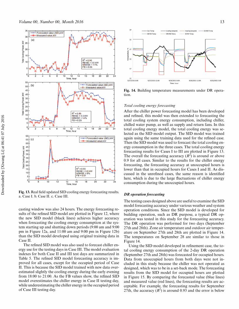
Fig. 13. Real field updated SID cooling energy forecasting results.a. Case I. b. Case II. c. Case III.

casting window was also 24 hours. The energy forecasting re-sults of the refined SID model are plotted in Figure 12, wherethe new SID model (black lines) achieves higher accuracywhen forecasting the cooling energy consumption at the sys-tem starting up and shutting down periods (9:00 am and 9:00pm in Figure 12a, and 11:00 am and 9:00 pm in Figure 12b)than the SID model developed using original training data inCase II.

The refined SID model was also used to forecast chiller en-ergy use for the testing days in Case III. The model evaluationindexes for both Case II and III test days are summarized inTable 5. The refined SID model forecasting accuracy is im-proved for all cases, except for the occupied period of CaseII. This is because the SID model trained with new data over-estimated slightly the cooling energy during the early eveningfrom 18:00 to 21:00. As the FB values show, the refined SIDmodel overestimates the chiller energy in Case II testing day,while underestimating the chiller energy in the occupied periodof Case III testing day.

Fig. 14. Building temperature measurements under DR opera-tion.

Total cooling energy forecastingAfter the chiller power forecasting model has been developedand refined, this model was then extended to forecasting thetotal cooling system energy consumption, including chiller,chilled water pump, as well as supply and return fans. In thistotal cooling energy model, the total cooling energy was se-lected as the SID model output. The SID model was trainedagain using the same training data used for the refined case.Then the SID model was used to forecast the total cooling en-ergy consumption in the three cases. The total cooling energyforecasting results for Cases I to III are plotted in Figure 13.The overall the forecasting accuracy (R2) is around or above0.9 for all cases. Similar to the results for the chiller energyforecasting, the forecasting accuracy at unoccupied hours islower than that in occupied hours for Cases I and II. As dis-cussed in the unrefined cases, the same reason is identifiedhere, which is due to the large fluctuations of chiller energyconsumption during the unoccupied hours.

DR operation forecasting

The testing cases designed above are useful to examine the SIDmodel forecasting accuracy under various weather and systemoperation conditions. Since the SID model is developed forbuilding operation, such as DR purpose, a typical DR op-eration was tested in this study for the forecasting accuracy.The DR operation was performed for two days (September27th and 28th). Zone air temperature and outdoor air temper-ature on September 27th and 28th are plotted in Figure 14.The temperatures on September 28 are similar to those inFigure 14.

Using the SID model developed in refinement case, the to-tal cooling energy consumption of the 2-day DR operation(September 27th and 28th) was forecasted for occupied hours.Data from unoccupied hours from both days were not in-cluded in this study because the chiller was not operated asdesigned, which was to be in a set-back mode. The forecastingresults from the SID model for occupied hours are plottedin Figure 15. By comparing the forecasted value (blue lines)and measured value (red lines), the forecasting results are ac-ceptable. For example, the forecasting results for September27th, the accuracy (R2) is around 0.93 and the error is below

Dow

nloa

ded

by [

Xiw

ang

Li]

at 0

6:41

07

July

201

6

14 Science and Technology for the Built Environment

Fig. 15. Total cooling energy forecasting for DR operation.

5% (RMSE = 2.5 kW and NRMSE = 3.1%). The forecastingresults for September 28th are also acceptable with R2 = 0.89,RMSE = 4.6 kW, and NRMSE = 5.3%. FB factors are above0 for both of these 2 days, which means that the SID modelstill tends to overestimate the energy consumptions during thisDR operation.

Model uncertainty analysis

A Monte Carlo (MC) simulation is conducted to analyze thenoise impact on model accuracy. During a MC simulation, thefollowing process is used:

1. Initialize MC simulation by defining input noise distribu-tions (+/–5%) and adding the noise to the “measurement;”

2. Perform MC: for i = 1. . .N (in this study, N is chosen as5000, suggested by (Eisenhower et al. [2012])• Sample noise values from defined distributions (in this

study, 5% Gaussian distributed random white noise isused)

• Run each model for energy forecasting• Calculate MC output (daily energy consumption, kWh)

3. Analyze the model performance.

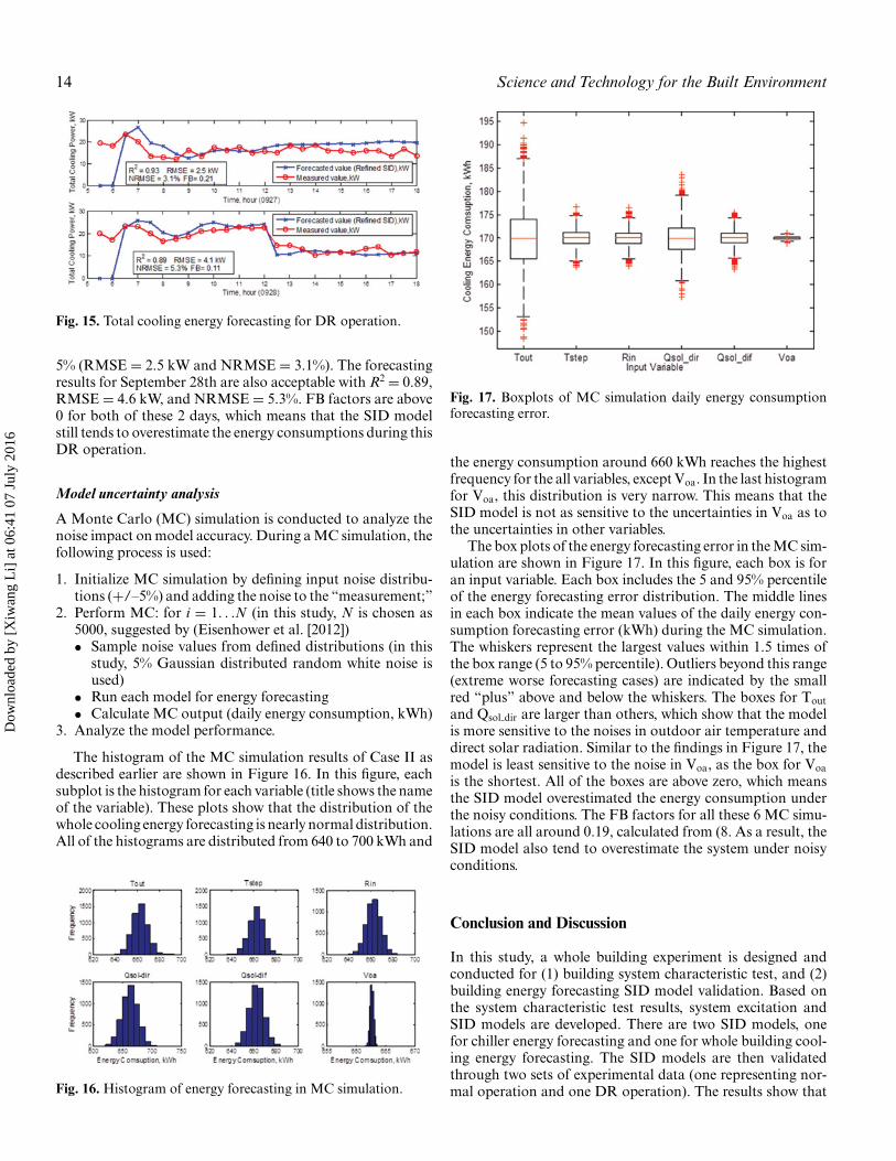
The histogram of the MC simulation results of Case II asdescribed earlier are shown in Figure 16. In this figure, eachsubplot is the histogram for each variable (title shows the nameof the variable). These plots show that the distribution of thewhole cooling energy forecasting is nearly normal distribution.All of the histograms are distributed from 640 to 700 kWh and

Fig. 16. Histogram of energy forecasting in MC simulation.

Fig. 17. Boxplots of MC simulation daily energy consumptionforecasting error.

the energy consumption around 660 kWh reaches the highestfrequency for the all variables, except Voa. In the last histogramfor Voa, this distribution is very narrow. This means that theSID model is not as sensitive to the uncertainties in Voa as tothe uncertainties in other variables.

The box plots of the energy forecasting error in the MC sim-ulation are shown in Figure 17. In this figure, each box is foran input variable. Each box includes the 5 and 95% percentileof the energy forecasting error distribution. The middle linesin each box indicate the mean values of the daily energy con-sumption forecasting error (kWh) during the MC simulation.The whiskers represent the largest values within 1.5 times ofthe box range (5 to 95% percentile). Outliers beyond this range(extreme worse forecasting cases) are indicated by the smallred “plus” above and below the whiskers. The boxes for Toutand Qsol dir are larger than others, which show that the modelis more sensitive to the noises in outdoor air temperature anddirect solar radiation. Similar to the findings in Figure 17, themodel is least sensitive to the noise in Voa, as the box for Voais the shortest. All of the boxes are above zero, which meansthe SID model overestimated the energy consumption underthe noisy conditions. The FB factors for all these 6 MC simu-lations are all around 0.19, calculated from (8. As a result, theSID model also tend to overestimate the system under noisyconditions.

Conclusion and Discussion

In this study, a whole building experiment is designed andconducted for (1) building system characteristic test, and (2)building energy forecasting SID model validation. Based onthe system characteristic test results, system excitation andSID models are developed. There are two SID models, onefor chiller energy forecasting and one for whole building cool-ing energy forecasting. The SID models are then validatedthrough two sets of experimental data (one representing nor-mal operation and one DR operation). The results show that

Dow

nloa

ded

by [

Xiw

ang

Li]

at 0

6:41

07

July

201

6

Volume 00, Number 00, Month 2016 15

the developed SID models have around or over 90% (R2) ac-curacy and less than 10% (NRMSE) error during occupiedhours for both chiller and total cooling energy forecasting.The SID model accuracy is lower during unoccupied or sys-tem starting-up periods, but is still above 85%. Overall, thedeveloped SID model tend to overestimate the energy usagesin all cases. The results from an uncertainty analysis demon-strates that the SID model is less sensitive to the uncertaintiesin ventilation flowrate, comparing with uncertainties in othersystem inputs, such as outdoor air temperature, temperatureset-points, etc. Applying this method to other commercialbuildings, this method will first conduct the system charac-teristic test to get the system response time and nonlinearity.Then system excitation signal will be generated based on thesystem response time and nonlinearity. Finally, the proposedSID methodology will develop the energy forecasting modelfor building operation.

On the other hand, there still are some limitations for thisstudy. First, for most of this experiment study, the facility isunder a testing operation. The operational data under normaloperation is only collected from the designed normal opera-tion days. Therefore, it is difficult to compare the performancewith other energy forecasting models, such as historical dataaverage method and regression models. Second, the active sys-tem excitation is needed to generate the model training data.The active system excitation can only conducted at uncopiedhours and weekends, which may also cause wear and teardegradation of the system. Finally, only one of the pre-coolingDR operation has been tested in this study due to the experi-ment schedules, the performance of this method in more DRoperation schemes are planned to further prove the superiorityof this proposed building energy forecasting methodology.

Going forward, more studies focusing the following direc-tions are needed:

1. In the system response time test, it is very hard to eliminatethe outdoor disturbances such as outdoor temperature andsolar radiation variations. More studies are needed on howto separate the system responses from inputs and fromdisturbances;

2. During a system’s excitation period, there are other vari-ables that could be excited, such as chilled water outlettemperature set-points, supply air temperature and pres-sure set-points, besides zone temperature set-points, andequipment schedules that are studied in this article. Morestudies are also needed to understand how to choose andexcite these variables.

Nomenclature

Cxy = nonlinear indexGxx = input variable auto power spectral densityGyy = output variable auto power spectral densityGxy = input and output variable cross power spectral

densitySuu = input auto power spectral density resultSyu = input and output variable cross power spectral

density resultG(z) = transfer function in frequency domain

G(t) = transfer function in time domainUτ = excitation signal at time τ

aτ = excitation function magnitude scale parameter attime τ

ωτ = periodic frequency parameterT = sampling timeϕτ = phase lag parameter at time τ

R2 = coefficient of determinationRMSE = root mean square errorNRMSE = normalized root mean square errorFB = fractional bias

Funding

The financial support that was provided by the U.S. Na-tional Science Foundation (Award ID: 1239247) is greatlyappreciated.

References

Agbi, C., Z. Song, and B. Krogh. 2012. Parameter identifiability formulti-zone building models. 2012 IEEE 51st Annual Conference onDecision and Control (CDC), December 10–13, Maui, HI.

Bacher, P., and H. Madsen. 2011. Identifying suitable models for the heatdynamics of buildings. Energy and Buildings 43(7):1511–22.

Braun, J.E. 2003. Load control using building thermal mass. Journalof Solar Energy Engineering-Transactions of the ASME 125(3):292–301.

Braun, J.E., and N. Chaturvedi. 2002. An inverse gray-box model fortransient building load prediction. HVAC&R Research 8(1):73–99.

Cai, J., D. Kim, J.E. Braun, and J. Hu. 2016. Optimizing zone temper-ature setpoint excitation to minimize training data for data-drivendynamic building models. American Control Conference, Submitted,Boston, MA, July 6–8.

Chen, H.-J., D.W.P. Wang, and S.-L. Chen. 2005. Optimization of anice-storage air conditioning system using dynamic programmingmethod. Applied Thermal Engineering 25(2–3):461–72.

Chen, X., Q. Wang, and J. Srebric. 2015. A data-driven state-space modelof indoor thermal sensation using occupant feedback for low-energybuildings. Energy and Buildings 91:187–98.

Cigler, J., and S. Priavara. 2010. Subspace identification and model pre-dictive control for buildings. 2010 IEEE 11th International Confer-ence on Control Automation Robotics & Vision (ICARCV), Singa-pore, December 7–10.

DOE. U.S. 2013. Buildings energy data book. http://buildings-databook.eren.doe.gov/.

Domınguez-Munoz, F., J.M. Cejudo-Lopez, and A. Carrillo-Andres.2010. Uncertainty in peak cooling load calculations. Energy andBuildings 42(7):1010–8.

Eisenhower, B., Z. O’Neill, V.A. Fonoberov, and I. Mezic. 2012. Un-certainty and sensitivity decomposition of building energy models.Journal of Building Performance Simulation 5(3):171–84.

Fux, S.F., A. Ashouri, M.J. Benz, and L. Guzzella. 2014. EKF based self-adaptive thermal model for a passive house. Energy and Buildings68(Part C):811–7.

Hazyuk, I., C. Ghiaus, and D. Penhouet. 2012. Optimal temperaturecontrol of intermittently heated buildings using model predic-tive control: part I—building modeling. Building and Environment51:379–87.

Henze, G.P., and R.H. Dodier. 2003. Adaptive optimal control of agrid-independent photovoltaic system. Journal of Solar Energy En-gineering 125(1):34–42.

Dow

nloa

ded

by [

Xiw

ang

Li]

at 0

6:41

07

July

201

6

16 Science and Technology for the Built Environment

Hu, M. 2015. A data-driven feed-forward decision framework forbuilding clusters operation under uncertainty. Applied Energy141:229–37.

Jain, R.K., K.M. Smith, P.J. Culligan, and J.E. Taylor. 2014. Forecast-ing energy consumption of multi-family residential buildings usingsupport vector regression: investigating the impact of temporal andspatial monitoring granularity on performance accuracy. AppliedEnergy 123:168–78.

Lee, K.-h., and J.E. Braun. 2008. Model-based demand-limiting controlof building thermal mass. Building and Environment 43(10):1633–46.

Lee, W.-S., Y.T. Chen, and T.-H. Wu. 2009. Optimization for ice-storageair-conditioning system using particle swarm algorithm. AppliedEnergy 86(9):1589–95.

Lee, Y.-S., and L.-I. Tong. 2012. Forecasting nonlinear time series ofenergy consumption using a hybrid dynamic model. Applied Energy94:251–6.

Lennart, L. 1999. System Identification: Theory for the User. Upper Sad-dle River, NJ: PTR Prentice Hall.

Li, X., and J. Wen. 2014a. Building energy consumption on-line forecast-ing using physics based system identification. Energy and Buildings82:1–12.

Li, X., and J. Wen. 2014b. Building Energy consumption on-line fore-casting using system identification and data fusion. ASME 2014Dynamic Systems and Control Conference (DSCC), San Antonio,Texas, October 22–24.

Li, X., and J. Wen. 2014c. Review of building energy modeling forcontrol and operation. Renewable and Sustainable Energy Reviews37:517–37.

Li, X., J. Wen, and E.-W. Bai. 2015a. Building energy forecasting us-ing system identification based on system characteristics test. IEEE2015 Workshop on Modeling and Simulation of Cyber-Physical En-ergy Systems (MSCPES), Seattle, WA, April 13.

Li, X., J. Wen, and T. Wu. 2015b. Comparison of on-line building energyforecasting model using system identification method and othermethods. 2015 ASHRAE Annual Conference Atlanta, GA, June 27–July 1.

Li, X., J. Wen, and E.-W. Bai. 2016. Developing a whole building coolingenergy forecasting model for on-line operation optimization usingproactive system identification. Applied Energy 164:69–88.

Lu, X., T. Lu, C.J. Kibert, and M. Viljanen. 2014. A novel dynamic mod-eling approach for predicting building energy performance. AppliedEnergy 114:91–103.

Lu, X., T. Lu, C.J. Kibert, and M. Viljanen. 2015. Modeling and fore-casting energy consumption for heterogeneous buildings using aphysical–statistical approach. Applied Energy 144:261–75.

Moon, J.W. 2012. Performance of ANN-based predictive and adaptivethermal-control methods for disturbances in and around residentialbuildings. Building and Environment 48:15–26.

Oldewurtel, F., A. Parisio, C.N. Jones, D. Gyalistras, M. Gwerder, V.Stauch, B. Lehmann, and M. Morari. 2012. Use of model predictivecontrol and weather forecasts for energy efficient building climatecontrol. Energy and Buildings 45:15–27.

Price, B.A., and T.F. Smith. 2000. Description of the Iowa Energy CenterEnergy Resource Station: facility update III. Technical Report ME-TFS-00-001, The University of Iowa.

Privara, S., J. Cigler, Z. Vana, F. Oldewurtel, C. Sagerschnig, and E.Zacekova. 2013. Building modeling as a crucial part for buildingpredictive control. Energy and Buildings 56:8–22.

Privara, S., Z. Vana, J. Cigler, and L. Ferkl. 2012. Predictive controloriented subspace identification based on building energy simula-tion tools. IEEE 2012 20th Mediterranean Conference on Control &Automation (MED), Barcelona, Spain, July 3–6.

Privara, S., Z. Vana, D. Gyalistras, J. Cigler, C. Sagerschnig, M. Morari,and L. Ferkl. 2011. Modeling and identification of a large multi-zone office building. 2011 IEEE International Conference on ControlApplications (CCA), Denver, CO, September 28–30.

Radecki, P., and B. Hencey. 2013. Online thermal estimation, control,and self-excitation of buildings. 2013 IEEE 52nd Annual Confer-ence on Decision and Control (CDC), Florence, Italy, December10–13.

Rivera, D.E., H. Lee, H.D. Mittelmann, and M.W. Braun. 2009. Con-strained multisine input signals for plant-friendly identificationof chemical process systems. Journal of Process Control 19(4):623–35.

Roldan-Blay, C., G. Escriva-Escriva, C. Alvarez-Bel, C. Roldan-Porta,and J. Rodrıguez-Garcıa. 2013. Upgrade of an artificial neuralnetwork prediction method for electrical consumption forecastingusing an hourly temperature curve model. Energy and Buildings60:38–46.

Touretzky, C.R., and R. Patil. 2015. Building-level power demand fore-casting framework using building specific inputs: development andapplications. Applied Energy 147:466–77.

Vaghefi, A., M.A. Jafari, E. Bisse, Y. Lu, and J. Brouwer. 2014. Modelingand forecasting of cooling and electricity load demand. AppliedEnergy 136:186–96.

Wang, S., and X. Xu. 2006. Simplified building model for tran-sient thermal performance estimation using GA-based parame-ter identification. International Journal of Thermal Sciences 45(4):419–32.

Xi, X.-C., A.-N. Poo, and S.-K. Chou. 2007. Support vector regressionmodel predictive control on a HVAC plant. Control EngineeringPractice 15(8):897–908.

Zervas, P., H. Sarimveis, J. Palyvos, and N. Markatos. 2008. Model-based optimal control of a hybrid power generation system consist-ing of photovoltaic arrays and fuel cells. Journal of Power Sources181(2):327–38.

Dow

nloa

ded

by [

Xiw

ang

Li]

at 0

6:41

07

July

201

6

Volume 00, Number 00, Month 2016 17

Appendix

Table A.1. Nonlinearity test signal: Temperature set-points.

Day 1 Day 2

Time Cooling set-point, ◦F Heating set-point, ◦F Cooling set-point, ◦F Heating set-point, ◦F

12:00 65.9 60.9 67.6 62.60:30 76.4 71.4 65.5 60.51:00 65.4 60.4 63.0 58.01:30 69.6 64.6 68.3 63.32:00 68.6 63.6 72.6 67.62:30 65.7 60.7 67.2 62.23:00 65.1 60.1 75.5 70.53:30 72.1 67.1 66.6 61.64:00 64.8 59.8 77.5 72.54:30 65.0 60.0 67.3 62.35:00 73.9 68.9 70.2 65.25:30 69.8 64.8 75.0 70.06:00 71.2 66.2 74.2 69.26:30 66.6 61.6 67.1 62.17:00 69.1 64.1 72.5 67.57:30 70.9 65.9 65.8 60.88:00 70.4 65.4 63.7 58.78:30 76.2 71.2 72.2 67.29:00 67.6 62.6 63.6 58.69:30 69.3 64.3 62.1 57.110:00 72.8 67.8 69.6 64.610:30 73.2 68.2 74.8 69.811:00 62.7 57.7 74.2 69.211:30 68.4 63.4 64.4 59.412:00 67.4 62.4 69.9 64.912:30 69.7 64.7 72.7 67.713:00 71.7 66.7 73.3 68.313:30 71.4 66.4 75.4 70.414:00 73.9 68.9 75.5 70.514:30 71.4 66.4 72.9 67.915:00 70.9 65.9 64.7 59.715:30 73.2 68.2 69.9 64.916:00 71.3 66.3 64.8 59.816:30 65.0 60.0 74.2 69.217:00 70.2 65.2 76.1 71.117:30 63.8 58.8 62.6 57.618:00 73.8 68.8 72.8 67.818:30 62.2 57.2 68.6 63.619:00 67.8 62.8 68.1 63.119:30 70.1 65.1 66.6 61.620:00 69.7 64.7 74.4 69.420:30 76.6 71.6 71.2 66.221:00 70.0 65.0 69.4 64.421:30 67.6 62.6 71.3 66.322:00 71.9 66.9 73.5 68.522:30 65.5 60.5 66.7 61.723:00 71.8 66.8 66.9 61.923:30 70.7 65.7 67.8 62.812:00 68.4 63.4 69.4 64.4

Dow

nloa

ded

by [

Xiw

ang

Li]

at 0

6:41

07

July

201

6

18 Science and Technology for the Built Environment

Table A.2. Nonlinearity test signal: Equipment schedule.

Day 1 Day 2

Time Stage Lighting Base board Stage Lighting Base board heat

12:00 5 Stage 1 and 2 Stage 1 3 Stage 1 and 2 Off0:30 3 Stage 1 and 2 Off 2 Stage 2 Off1:00 2 Stage 2 Off 5 Stage 1 and 2 Stage 11:30 4 Off Stage 1 2 Stage 2 Off2:00 3 Stage 1 and 2 Off 5 Stage 1 and 2 Stage 12:30 4 Off Stage 1 4 Off Stage 13:00 2 Stage 2 Off 3 Stage 1 and 2 Off3:30 6 Off Stage 2 6 Off Stage 24:00 1 Stage 1 Off 5 Stage 1 and 2 Stage 14:30 7 Stage 1 and 2 Stage 2 2 Stage 2 Off5:00 5 Stage 1 and 2 Stage 1 1 Stage 1 Off5:30 2 Stage 2 Off 5 Stage 1 and 2 Stage 16:00 0 Off Off 3 Stage 1 and 2 Off6:30 5 Off Off 7 Stage 1 and 2 Stage 27:00 1 Stage 1 Off 3 Stage 1 and 2 Off7:30 6 Off Stage 2 6 Off Stage 28:00 6 Off Stage 2 3 Stage 1 and 2 Off8:30 5 Stage 1 and 2 Stage 1 3 Stage 1 and 2 Off9:00 5 Stage 1 and 2 Stage 1 2 Stage 2 Off9:30 2 Stage 2 Off 4 Off Stage 110:00 2 Stage 2 Off 2 Stage 2 Off10:30 5 Stage 1 and 2 Stage 1 2 Stage 2 Off11:00 3 Stage 1 and 2 Off 4 Off Stage 111:30 2 Stage 2 Off 5 Stage 1 and 2 Stage 112:00 5 Stage 1 and 2 Stage 1 2 Stage 2 Off12:30 6 Off Stage 2 2 Stage 2 Off13:00 2 Stage 2 Off 0 Off Off13:30 2 Stage 2 Off 2 Stage 2 Off14:00 7 Stage 1 and 2 Stage 2 6 Off Stage 214:30 4 Off Stage 1 2 Stage 2 Off15:00 1 Stage 1 Off 7 Stage 1 and 2 Stage 215:30 5 Stage 1 and 2 Stage 1 4 Off Stage 116:00 2 Stage 2 Off 3 Stage 1 and 2 Off16:30 5 Stage 1 and 2 Stage 1 5 Stage 1 and 2 Stage 117:00 5 Stage 1 and 2 Stage 1 2 Stage 2 Off17:30 2 Stage 2 Off 4 Off Stage 118:00 7 Stage 2 Stage 2 3 Stage 1 and 2 Off18:30 1 Stage 1 and 2 Off 5 Stage 1 and 2 Stage 119:00 3 Stage 1 and 2 Off 0 Off Off19:30 6 Off Stage 2 1 Stage 1 Off20:00 5 Stage 1 and 2 Stage 1 6 Off Stage 220:30 5 Stage 1 and 2 Stage 1 6 Off Stage 221:00 4 Off Stage 1 0 Off Off21:30 2 Stage 2 Off 5 Stage 1 and 2 Stage 122:00 4 Off Stage 1 4 Off Stage 122:30 0 Off Off 1 Stage 1 Off23:00 4 Off Stage 1 2 Stage 2 Off23:30 2 Stage 2 Off 1 Stage 1 Off12:00 6 Off Stage 2 4 Off Stage 1

Dow

nloa

ded

by [

Xiw

ang

Li]

at 0

6:41

07

July

201

6