building recognition using computer vision for urban ubiquitous environments · 2005-05-30 ·...
TRANSCRIPT
Building Recognition using Computer Vision
for Urban Ubiquitous Environments
Kenneth O’Hanlon
A dissertation submitted to the University of Dublin, in partial fulfilment of the requirements for the degree of
Master of Science in Computer Science (Ubicom)
2005

ii
Declaration
I declare that the work described in this dissertation is, except where otherwise stated, entirely my own work, and has not been submitted as an exercise for a degree at this or any other university.
Signed: Kenneth O’Hanlon 13 / 05 / 05

iii
Permission to lend and/or copy
I agree that the Trinity College Library may lend or copy this dissertation upon request.
Signed: Kenneth O’Hanlon 13/05/05
iv
Abstract
Mobile computing devices are becoming ever more powerful and smarter, and are
being seen with an increasingly diverse array of peripherals devices attached. Many
new mobile phones and PDAs have the ability to communicate using several different
wireless media.
Much research is in effect with regards to the development of Urban models; Virtual
Cities, and the linking of these to Geographical Information Systems, as well as other
knowledge bases. In this way the power of mobile computing may be enhanced, by
the provision of location-based and other services to mobile users.
Computer Vision applications are emerging from the domains of industry and
surveillance, and applications of such are becoming more common within the public
arena.
This project aims to demonstrate the feasibility of using Computer Vision as a user-
friendly technology, capable of recognising buildings. This recognition step will allow
users to access services, such as navigation and tourism information, by using
cameras embedded in mobile communications devices.

v
Acknowledgements
I would like to thank Dr. Kenneth Dawson-Howe, my dissertation project supervisor,
for all his help and guidance in the process of this project.
I would also like to thank the other group members, Yaou Li & Colm Conroy for their
encouragement, assistance and . I would like to thank them also for the brainstorming
process from which the idea for the amalgamated project emerged. On the same note I
express my sincerest gratitude to Stefan Weber; for suffering us and assisting to pull
the separate strands together; Declan O’Sullivan for enabling the bigger picture to
become apparent, and again Dr. Kenneth Dawson-Howe for the initial idea of using
vision techniques for building recognition. I also express earnest appreciation for the
time and effort expended by other members of the Computer Science Department who
we approached during the early days of this project. However, this list is probably too
long to fit in this dissertation.
On a more personal note I would like to thank my friends and family for all their
support during a period in which I must have seemed extremely preoccupied, and for
listening when I needed to let of steam.
Last but not least, I’d like to thank my girlfriend Elaine for persisting with me through
all those times when it seemed the only relationship I was part of included a PC.
vi
Table of Contents
Chapter 1: Introduction ...........................................................................1
Chapter 2 : Background...........................................................................6
2.1 Relevant works:..................................................................................................6 2.2 Discussion of Techniques of relevance ...........................................................12
2.2.1 Line Detection.............................................................................................12 2.2.2 Consistent Line Clustering..........................................................................13 2.2.3 Perceptual Grouping ...................................................................................14 2.2.4 Vanishing Point Detection ..........................................................................14 2.2.5 Perspective Rectification ............................................................................16
Chapter 3 : Design ..................................................................................18
3.1 Proposition and Rationale ...............................................................................18 3.2 Bigger Picture...................................................................................................19 3.3Tools ...................................................................................................................20 3.4Constraints Imposed .........................................................................................20
Chapter 4 : Algorithm Definition..........................................................22
4.1 Smoothing .........................................................................................................23 4.2 Edge Detection..................................................................................................24 4.3 Non maxima suppression ................................................................................26 4.4 Hysterisis Thresholding...................................................................................27 4.5 Edge Linking / Line segment Detection .........................................................28 4.6 Collinearity Detection ......................................................................................30 4.7 Line Clustering.................................................................................................31 4.8 Vanishing Point Detection ...............................................................................32 4.9 Perceptual Grouping .......................................................................................32
Chapter 5 : Implementation ..................................................................33
5.1 Edge Detection & Non-maxima suppression.................................................33 5.2 Adaptive Hysterisis Thresholding ..................................................................43 5.3 Edge Linking ....................................................................................................45 5.4 Collinearity .......................................................................................................50 5.5 Vanishing Point Detection ...............................................................................54
Chapter 6 : Conclusions .........................................................................60
Appendix A : References........................................................................61
Appendix B : Framework Overview.....................................................64
1 Information Eye ..................................................................................................64 2 Overall Framework Overview ...........................................................................64
vii
Table of Illustrations Figure 1:Averaging filter mask ______________________________________________________23 Figure 2: Prewitt Edge detector masks ________________________________________________25 Figure 3: Original Image___________________________________________________________33 Figure 4: Smoothed Image__________________________________________________________34 Figure 5: Edge map of building image ________________________________________________35 Figure 6: Orientation map of building image ___________________________________________36 Figure 7: Non maxima suppression using directions _____________________________________37 Figure 8: Effect of using angle-based non-maxima suppression. ___________________________37 Figure 9: Effect of combining both non-maxima suppression on lines parallel to axes __________38 Figure 10: Laplacian of Gaussian____________________________________________________39 Figure 11: Convolution masks_______________________________________________________40 Figure 12: Zero Crossing of Laplacian of Gaussian _____________________________________41 Figure 13:Merged Detectors ________________________________________________________42 Figure 14: Thresholded Edge Map after Adaptive Hysterisis_______________________________44 Figure 15: Edge linking(Colours apply to different edges)_________________________________46 Figure 16: Merged Edges___________________________________________________________49 Figure 17: Collinear Segments ______________________________________________________51 Figure 18: Line segments clustered by orientation _______________________________________52 Figure 19:Thresholded image showing all lines created through collinearity search____________53 Figure 20: Intensity image showing lines created through intensity search ___________________53 Figure 21: Lines cluster according to angle ____________________________________________56 Figure 22: Line Clusters after further clustering by line weight____________________________57 Figure 23: Lines going to vanishing point _____________________________________________58 Figure 24:Line Segments belonging to vanishing lines ___________________________________58

1
Chapter 1: Introduction
Computer Vision is a field of Computer Science, in which an understanding of the
environment is sought through the processing of images.
Ubiquitous Computing is an emerging field, encompassing the ideas of mobile
computing, knowledge-based and sensor-driven context awareness, and aspiring
towards a multi-modal user-machine interaction.
1.1 Aims
The aim of this project, as an individual piece of work, is to demonstrate the
feasibility of using Computer Vision techniques to recognise buildings. This is a base
technology, which could have many potential uses as an interface in outdoor
Ubiquitous Computing environments.
This project is part of a larger intended framework, titled “Information Eye”. This is a
collaborative effort, consisting of two other dissertation projects. The goal of this
speculative framework is to enable users to locate desired services in an urban area.
Yaou Li intends to show how a geographic information system can be based in an
ontology, how this can be linked to other information sources related to the area, and
demonstrate how users might locate services in such a space. Colm Conroy intends to
show how separate ontologies might be mapped to each other, allowing semantic
interoperability across different domains. The author intends to show the feasibility of
the use of the camera as an interface to this information space through recognition of
buildings in the space.
2
1.2 Motivation
Computer Vision has been successful in many applications. Until recently, the
locations of most of these applications were within very constrained environments,
typically in industrial settings. Many production lines contain a computer vision
element at some stage, as either a control element for a mechanical part, or as a
quality-classifying instrument. However, for now, there is no generic solution to
Computer Vision, and most experts would agree that one is not fast approaching.
Most Vision applications are specifically tailored to the environment in which they
operate, and cameras are usually set to operate within a fixed location domain.
The level of intelligence in Vision programs is increasing. New technologies from the
Computer Vision family include face recognition and gait recognition.
Recent developments have seen Computer Vision brought forward as a user
interactive technology. Cameras are often used in prototype multi-modal interaction
systems as a computer interface, allowing gesture recognition to be combined with,
for instance, a speech interface. Although these interfaces have not been perfected,
large strides have been made towards achieving these goals. An example of the
emergence of Computer Vision into the public domain is the “Eye Toy”. This was
introduced a year ago as an interface for the Playstation 2, allowing games to be
completely controlled by a user’s motions, as sensed by a small USB camera.
Augmented Reality is one of the constituent fields of Ubiquitous Computing. In an
Augmented Reality system, digital components are added to real-world scenarios.
3
Many AR systems include the use of transparent head-mounted displays, allowing
digital graphic elements to be augmented to a user’s field of view, against the
background of ‘reality’. Other AR systems are less advanced, the interface
constituting a PDA and a camera. In these systems the PDA display may consist of
the camera image with text or other information annotated. Typically, vision-based
augmented reality systems rely on the placement of patterned black-and-white
markers in the environment, reducing the time taken in the recognition stage, and the
environment modelling required.
AR is an active field of research. One of the primary visions of usage of augmented
reality is in gaming systems. Several prototypes games have been developed. Some
researchers have noted the time lag inherent in such systems, due to the heavy
processing load, which is caused by first having to process an image, from which
bearings may be calculated, and then infer the position of the augmented elements
relative to these bearings. This is particularly detrimental to the fluidity required for
such a highly interactive environment such as a game. This issue may be resolved in
the future with the increasing speed of processors, and particularly if custom hardware
is built for these applications. One only has to look at the growth in graphics
capabilities through custom hardware in recent times, which can be partially
explained by the lucrative state of the gaming industry. Such a growth in image
processing hardware capabilities would surely benefit the greater field of Computer
Vision as well.
However, Augmented reality in less demanding, less interactive environments is
possible today. Telepointing is one such application. In a telepointing system a user
4
may point a sensor at an object and then receive information about this object,
typically to a PDA, although other interfaces such as audio are possible. A
Telepointing infrastructure may be based on different sensors. In [1] a telepointing
prototype was built using a camera with other sensors, namely GPS, a digital compass
and a tilt sensor. In this application, the vision system was the central element, whilst
the other sensors were incorporated to decrease the search space of the vision
algorithm within a full-scale 3D virtual model of the environment. The user was able
to divine information about buildings that they had pointed at, whilst also increasing
the accuracy of their location. An interesting facet of this augmented reality project
was that the objects of interest to the vision system were real-world objects such as
buildings.
In [2] Wagner & Schmalsteig introduce the “first standalone Augmented Reality
system ….. running on a unmodified PDA with a commercial camera”. Their paper
describes an application running on a PDA, which allows a user to be guided around
an unknown building by optical tracking using signposts (black and white markers).
Each marker is distinctive and indicates a specific location. From this inferred
location, the direction to the desired location may be ascertained. Whilst the camera
was small (320 * 240 pixels) and slow (6.2 frames per second), the authors have
claimed that the application runs in “interactive time”. Further work described in the
paper illustrates the offloading of some of the processing work to servers via WLAN.
Many virtual city models have been built, or are in the process of being built.
Wireless network infrastructures are starting to populate urban areas. The mobile
phone and the PDA are both progressing fast in processing power and are becoming

5
more similar. Many new phones possess 802.11 or Bluetooth capabilities. Many new
PDAs possess GSM or even 3G capabilities. New functionality and peripherals are
constantly being added, and recently a phone with a hard drive has been released.
In light of these fast-emerging technologies, it is not hard to predict, that over the
course of a few years, full scale urban ubiquitous environments will become a reality.
A question remains as to how interaction with these environments will take place.
One such possibility is camera-based interaction. Most new mobile devices now
include a camera, and even current wireless bandwidths would allow images to be
transmitted quickly.
Whilst not trying to foresee the day when architects are required to include black and
white markers as a requisite in their designs, to allow for augmented reality
infrastructures, this project endeavours to develop a simple method for recognition of
buildings within an environment without the need of a full scale 3D environment and
extensive auxiliary sensing.
6
Chapter 2 : Background
This sections aims to relate to the reader current research into building recognition,
underpinning the approach taken in this project. Although a relatively sparse field of
research, different approaches have been taken to the task of recognition of buildings
in images. The motivations for this work, too, have been varied.
Encouragement too has been drawn from architectural photogrammetry research.
Although mostly concerned with the reconstruction of buildings from images, and
with automation not being a necessary element in this approach, a wealth of
methodology exists in this field, which may be cultivated for the purpose of building
recognition.
2.1 Relevant works:
Much of the research in building recognition has taken place within the field of
content-based image retrieval. Rather than recognising a building per se, this research
has focused on recognising that there is a building, or more accurately stated, a man-
made structure in the image. Various approaches have been taken to this problem.
However the basis of this most of these techniques is that man-made structures, for
the main part, are considerably more ordered than natural objects, and therefore that
images containing man-made structures will contain more ‘order’, in terms of straight
lines and patterns.
Iqbal & Aggarwal [3][4] in two papers describe the method of perceptual grouping,
and it’s application to identification of manmade structures in images. Building
7
detection using perceptual grouping is an emerging area of the application of the
Gestalt laws of psychology to computer vision[3].
In these papers the authors describe how they define different image features that are
considered indicative of man-made structures. These features include straight-line
segments, co-terminations, L-junctions, U-junctions, and polygons. Further indication
of structure is provided by parallelism between these features and groups of these
features.
Zhou, Rui & Huang in [5] relate their water-filling algorithm for structural feature
extraction from images. The water-filling algorithm is a method for feature extraction
from a binary edge map of an image without using edge linking or shape
representation. Experimental results were promising.
Li & Shapiro[6] introduce the idea of consistent line clusters to detect buildings. In
their implementation, an edge map is searched for line segments.
“An important characteristic of buildings is that they contain many line segments,
often horizontal and vertical, which come from the boundaries of the windows, the
doors, or the building itself”[6].
These lines are then clustered based on colour, orientation and spatial features. Once
clustered, the inter- and intra- relationships of the line clusters are tested. The inter-
relationship queries intersections of a given line segment with other lines that have
been extended. These intersections indicate junctions. The intra-relationship queries
overlapping line segments in the building i.e. looks for collinearity in the image,
another indicator of structure, and hence the presence of a building in an image.
8
Recognition of a particular building from an image is a research area in which not a
lot of previous work has been done. Zhang & Kosecka[5] report knowing of only one
other body of work in this field, that of Bohm & Haala[1][8][9]. Having found a few
other bodies of work, it is possible to define these works as belonging to one of two
categories. The first category considers recognition of buildings from keypoint / scale-
invariant feature detection. The second category recognises buildings by comparison
with relatively extensive 3D models, and may employ extra sensors to limit the search
space.
Zhang and Kosecka present an approach to identifying buildings in images based on
keypoints or local scale-invariant features[7]. Their approach to feature detection is
modelled on that of Lowe[10 ]. Buildings are represented or modelled by the presence
of such scale-invariant features, which are features or “image locations which can be
detected efficiently and have been shown to be stable across wide variations of
viewpoint and scale”[7]. A database of buildings modelled as such was built.
Presented query images were then modelled as such and compared for similarity with
each image in the database. Problems identified included occlusion by natural objects,
such as trees; the presence of more than one building in an image; large out-of-plane
rotation and difference in lighting conditions between reference and test images. A
problem identified of particular note is that of mismatches caused by repeating
structures.
At IBM the “InfoScope” project could be considered a truly ubiquitous computing
project, linking “Real World to Digital Information Space”[11]. In this paper
Haritaoglu describes the use of computer vision as part of two applications. The first
9
of these applications extracts text information from real-world scenes and translates
these into the language of the user. Processing steps include
• Scene text detection
• Character segmentation
• Character recognition
• Language translation
• Text augmentation of the user interface.
Similar work relating to the computer vision aspects of this application i.e. the first
three steps mentioned above has been performed by Chen & Yuille[12]. Furthering
this Jung et al [13] have performed similar work, with the extension that their work
concentrates on wide text sequences which need be extracted from an image
sequence.
The second application in the InfoScope project enables users to see information
related to a building overlaid on a real scene image. From a PDA, a user selects the
building of interest in the image by placing a bounding box around it with a stylus.
GPS was also integrated into the system, with the stated intention to counter the false
positives that may be produced when searching a large database. GPS enables the
search space to be scaled down to a small number of buildings in the vicinity of the
user. The building recognition algorithm used was based on RGB colour similarity
with edge orientation similarity.
Bohm & Haala[1][8][9] have developed a seemingly extensive system using a CAD
model to represent buildings. The CAD model consists of polyhedrons, with no
texture information attached.
10
In this system the user is equipped with a camera, a GPS module, a digital compass
and a tilt sensor. As in InfoScope the GPS system is used to diminish the search space
of the user. The digital compass further enhances this ability by limiting the search
space to buildings in a particular direction, from the location identified by GPS.
Ideally this information would be enough to ascertain the building to be selected from
the CAD database.
Furthering this again the tilt sensor provides information about the orientation to
ground at which an image is produced. This allows the CAD model to be queried with
information with camera angle as well, allowing a perspective view of the outline of
the building to be produced. This outline is then compared against the image taken
from the camera. The Generalized Hough Transform is used to detect the building in
the image. The transform returns a “similarity transform consisting of translation,
rotation and scale. This transform corrects for the misalignment of the shape to it’s
actual appearance in the image”[9]. Using this information, it is possible to correct for
the sensor data, allowing the system to be used as an accurate location sensor.
This accuracy was tested by comparing the co-ordinates obtained solely through GPS,
the co-ordinates obtained from the complete system, and the co-ordinates on a high
resolution digital map when the photos where taken from distinguishable locations. It
was recorded that the Z-plane information from the GPS module was not used, this
information being replaced by elevation measurements from a digital map [9]. The
camera-based system improved the location accuracy each time this was tested. This
system seemed technically very impressive, but very costly in terms of both
equipment and processing. The detection of the overall shape of buildings of course
requires a sufficient distance of the user to the depicted building [1]. Although the
11
authors state that this should not be problematic for applications such as telepointing,
it is conceivable that there are areas in cities where a skyline is hard to define.
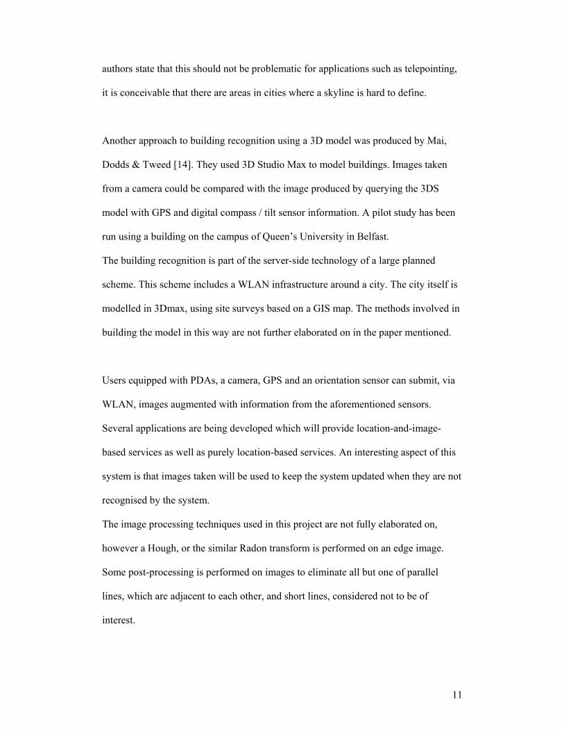
Another approach to building recognition using a 3D model was produced by Mai,
Dodds & Tweed [14]. They used 3D Studio Max to model buildings. Images taken
from a camera could be compared with the image produced by querying the 3DS
model with GPS and digital compass / tilt sensor information. A pilot study has been
run using a building on the campus of Queen’s University in Belfast.
The building recognition is part of the server-side technology of a large planned
scheme. This scheme includes a WLAN infrastructure around a city. The city itself is
modelled in 3Dmax, using site surveys based on a GIS map. The methods involved in
building the model in this way are not further elaborated on in the paper mentioned.
Users equipped with PDAs, a camera, GPS and an orientation sensor can submit, via
WLAN, images augmented with information from the aforementioned sensors.
Several applications are being developed which will provide location-and-image-
based services as well as purely location-based services. An interesting aspect of this
system is that images taken will be used to keep the system updated when they are not
recognised by the system.
The image processing techniques used in this project are not fully elaborated on,
however a Hough, or the similar Radon transform is performed on an edge image.
Some post-processing is performed on images to eliminate all but one of parallel
lines, which are adjacent to each other, and short lines, considered not to be of
interest.
12
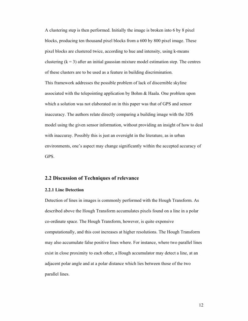
A clustering step is then performed. Initially the image is broken into 6 by 8 pixel
blocks, producing ten thousand pixel blocks from a 600 by 800 pixel image. These
pixel blocks are clustered twice, according to hue and intensity, using k-means
clustering (k = 3) after an initial gaussian mixture model estimation step. The centres
of these clusters are to be used as a feature in building discrimination.
This framework addresses the possible problem of lack of discernible skyline
associated with the telepointing application by Bohm & Haala. One problem upon
which a solution was not elaborated on in this paper was that of GPS and sensor
inaccuracy. The authors relate directly comparing a building image with the 3DS
model using the given sensor information, without providing an insight of how to deal
with inaccuray. Possibly this is just an oversight in the literature, as in urban
environments, one’s aspect may change significantly within the accepted accuracy of
GPS.
2.2 Discussion of Techniques of relevance
2.2.1 Line Detection
Detection of lines in images is commonly performed with the Hough Transform. As
described above the Hough Transform accumulates pixels found on a line in a polar
co-ordinate space. The Hough Transform, however, is quite expensive
computationally, and this cost increases at higher resolutions. The Hough Transform
may also accumulate false positive lines where. For instance, where two parallel lines
exist in close proximity to each other, a Hough accumulator may detect a line, at an
adjacent polar angle and at a polar distance which lies between those of the two
parallel lines.
13
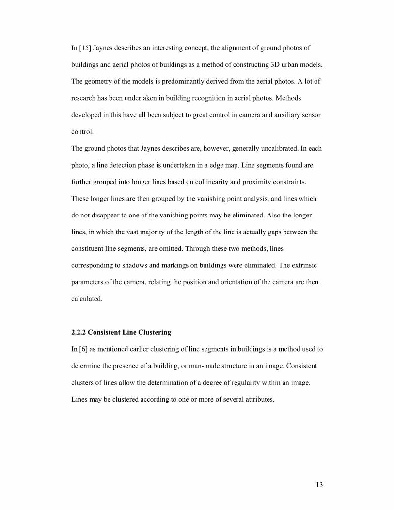
In [15] Jaynes describes an interesting concept, the alignment of ground photos of
buildings and aerial photos of buildings as a method of constructing 3D urban models.
The geometry of the models is predominantly derived from the aerial photos. A lot of
research has been undertaken in building recognition in aerial photos. Methods
developed in this have all been subject to great control in camera and auxiliary sensor
control.
The ground photos that Jaynes describes are, however, generally uncalibrated. In each
photo, a line detection phase is undertaken in a edge map. Line segments found are
further grouped into longer lines based on collinearity and proximity constraints.
These longer lines are then grouped by the vanishing point analysis, and lines which
do not disappear to one of the vanishing points may be eliminated. Also the longer
lines, in which the vast majority of the length of the line is actually gaps between the
constituent line segments, are omitted. Through these two methods, lines
corresponding to shadows and markings on buildings were eliminated. The extrinsic
parameters of the camera, relating the position and orientation of the camera are then
calculated.
2.2.2 Consistent Line Clustering
In [6] as mentioned earlier clustering of line segments in buildings is a method used to
determine the presence of a building, or man-made structure in an image. Consistent
clusters of lines allow the determination of a degree of regularity within an image.
Lines may be clustered according to one or more of several attributes.
14
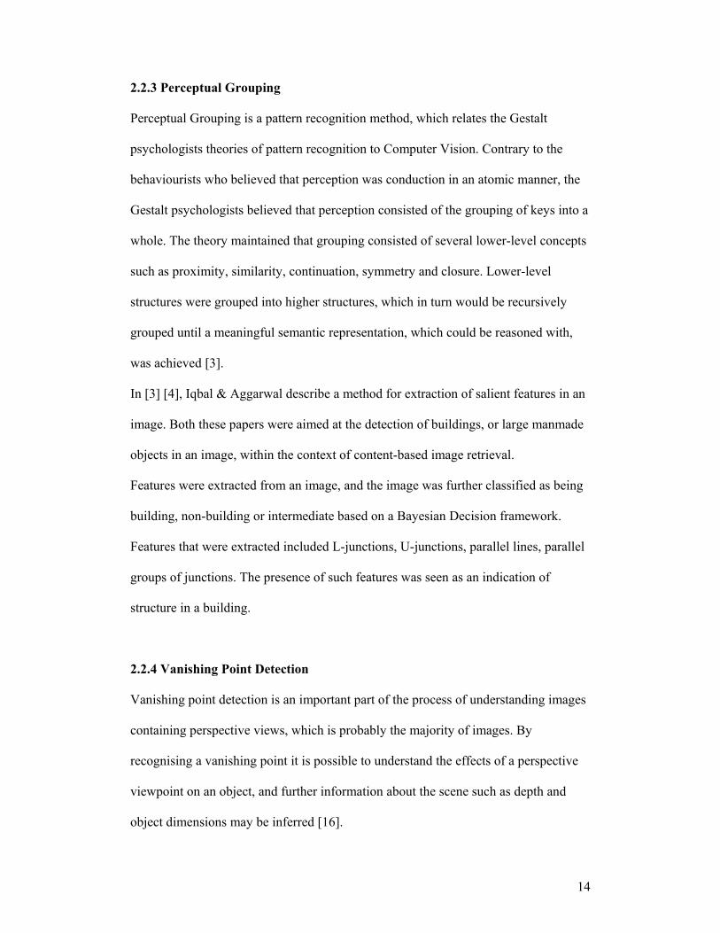
2.2.3 Perceptual Grouping
Perceptual Grouping is a pattern recognition method, which relates the Gestalt
psychologists theories of pattern recognition to Computer Vision. Contrary to the
behaviourists who believed that perception was conduction in an atomic manner, the
Gestalt psychologists believed that perception consisted of the grouping of keys into a
whole. The theory maintained that grouping consisted of several lower-level concepts
such as proximity, similarity, continuation, symmetry and closure. Lower-level
structures were grouped into higher structures, which in turn would be recursively
grouped until a meaningful semantic representation, which could be reasoned with,
was achieved [3].
In [3] [4], Iqbal & Aggarwal describe a method for extraction of salient features in an
image. Both these papers were aimed at the detection of buildings, or large manmade
objects in an image, within the context of content-based image retrieval.
Features were extracted from an image, and the image was further classified as being
building, non-building or intermediate based on a Bayesian Decision framework.
Features that were extracted included L-junctions, U-junctions, parallel lines, parallel
groups of junctions. The presence of such features was seen as an indication of
structure in a building.
2.2.4 Vanishing Point Detection
Vanishing point detection is an important part of the process of understanding images
containing perspective views, which is probably the majority of images. By
recognising a vanishing point it is possible to understand the effects of a perspective
viewpoint on an object, and further information about the scene such as depth and
object dimensions may be inferred [16].
15
Vanishing point detection is a generally statistical analysis due to inaccuracy in line
estimation in images. Usually vanishing point detection is carried out in the image
(x, y) space. Sets of lines can be seen to converge towards a point, which is the
vanishing point. Estimation of this point may be conducted in several similar
manners, generally requiring least squares analysis.
The points of intersection of all lines that disappear in a certain direction can be
determined. Taking the centroid of these intersection points, it is possible to eliminate
lines that are furthest from this centroid. The centroid may be recalculated at the
movement of the centroid recorded. This practice is repeated until the movement of
the centroid between iterations is below a threshold value. The advantage of this
method is that the result gives a set of lines that vanish to a point, as well as the co-
ordinates of this point to a certain degree of certainty. Alternatively, instead of
eliminating lines, it is feasible to eliminate in a similar manner.
Van den Heuvel [17] describes constructing a model from an image, and some
knowledge of the dimensions, of a building that was destroyed in the Second World
War. With the a priori knowledge of the building, it was possible to calibrate the
camera from vanishing point detection, two full faces of the building being visible in
the image. His vanishing point detection algorithm included all lines in the building
image, without prior separation due to orientation. He describes the statistical testing
of three lines simultaneously. One of these lines was fixed, and was the largest line in
the image. The results of this testing enabled the clustering of lines, the largest of
which corresponded to the lines which vanished to vanishing point of the original
largest line. These lines were then eliminated and the procedure repeated, until all
vanishing points were discovered.
16
In two papers [16][18], a vanishing point detection method, which operates in the
Hough Transform was described. While most vanishing point detection methods
operate in the image space, the Hough Transform operates in the polar space, each
line being described by the distance to the point in the line that is nearest to the origin
and by the angle taken to this point. In the Hough Transform, votes are accumulated
for each pixel lying in a line defined by (ρ,θ) coordinates. Lines present in the image
space should relate to points in the Hough space. Two lines, which intersect in the
image space, relate to two points in the Hough space both lie on the same sine arc. In
this approach, a vanishing point which is the intersection of several or many lines,
should defined by a sine arc. It was stated that this approach had only been tried on
images, which contained a vanishing point within, and that for detection of vanishing
points outside the image that the Hough space would have to be increased. Also work
had concentrated on images with one vanishing point.
In [16] Cantoni, Luca et al describe another method for vanishing point estimation,
this technique operating in the image space. Using two standard 3x3 isotropic edge
detection masks, an edge map is defined. A very high threshold is applied to this map,
resulting in a binary map. The orientation of the line is then calculated and a line is
passed through the point at the angle defined by the orientation. These lines are
accumulated in the (x, y) space. However it seems this process could be sensitive to
noise in the evaluation of the orientation from the two masks.
2.2.5 Perspective Rectification
Perspective rectification is an essential process in understanding the content of images
of three-dimensional objects. After undergoing a perspective rectification, it will be
possible to view individual planes of an image in a plan / elevation architectural
17
drafting style. Pattern recognition within each plane is then a more straightforward
process.
3D perspective rectification depends on fixed knowledge of one of two parameters. If
there is a priori knowledge of the dimensions of the object in the image, it is possible
to rectify the image with respect to these dimensions [17]. When this knowledge is
present it is possible to calibrate the camera from the vanishing points and the
information relating to the building [17].
Where this knowledge is not available, some camera calibration is necessary. In this
case it is necessary to know the intrinsic properties of the camera. Use of either of
these methods to perform 3D rectification requires the initial process of vanishing
point detection.
Forstner & Gulch [19] describe briefly the requirements of a camera calibration
procedure without using a test field with target points. The domain must be structured,
with well identifiable points, which can be identified in an image. They also state that
this calibration will not be as accurate as calibration in a test field, but that the
accuracy should be sufficient for the purpose of reconstruction or rectification of a
scene. The next section in the same paper describes how to determine the rotation
matrix of a plane from three line segments in that plane, two of which vanish to a
horizontal vanishing point, while the other vanishes to the azimuth.
Finally, in [20] Van den Heuvel describes a method for pose estimation, which can be
used for perspective rectification. This paper describes a method of using the points of
a rectangle, or parallelogram in object space to estimate the pose of the image. In
object space the triangles created by bisecting the rectangle in object space, must be
of equal area. This knowledge may be used to determine the perspective distortion
needed to rectify the image, assuming unit aspect ratio of the camera.
18
Chapter 3 : Design
3.1 Proposition and Rationale
As seen in the background section, different approaches have been taken to building
recognition within different frameworks. To generalise, these projects can be broken
into two categories; those that were concerned with the detection of a building in an
image; those that tried to recognise an actual building.
Projects belonging to the first category were concerned with content image-based
retrieval, and no other information was required to accompany the image. Methods
such as line-based clustering and perceptual grouping were performed in an attempt to
deduce the existence of structure in an image, in collaboration with a further decision-
making process.
The second category of projects attempted to confirm the actual buildings from a
known database of buildings. These projects included the use of extensive auxiliary
sensing equipment to locate the user in the real world before transferring these
coordinates into a digital virtual world to validate the scene or user location.
Only one project [7] actually attempted to recognise buildings from a database,
without other cues. This project used keypoints or scale-invariant features as a basis
for recognition of a building. However significant problems were registered with
lighting scenarios, repeating structures in buildings and others.
Based on these findings, this dissertation project attempts to demonstrate the viability
of using methods expressed in the first category of projects, such as line clustering
and perceptual grouping, as the basis of a building recognition system. As seen in [15]
19
the use of line clustering can overcome problems asserted by lighting and shadows,
whilst perceptual grouping thrives in the presence of repeating structures.
3.2 Bigger Picture
A well-developed building recognition system, built upon the fundamentals of this
project, could naturally extend into virtual city systems such as those expressed in the
second category of projects above, allowing use of services provided by such systems,
without the use of the extensive sensing equipment by users. A search space may be
reduced by location identification through the mobile infrastructure. The nearest cell
in a GSM or 3G network might presently define such location. However with the
large-scale deployment of urban wireless infrastructures such as WAND in Dublin,
this location might be expressed by systems such as LOCADIO[21] which is based on
signal strengths from wireless transmitters.
A knowledge system would be required, which could describe patterns as found in
building facades in terms of perceptual groupings. Another requirement of this system
is that it would enable reasoning with three dimensional data. Inference from a
database using such a knowledge system would need to be robust enough to allow for
recognition in images containing only part of a building, images containing more than
one building and, in particular would need to be able to deal with occlusion of parts of
buildings by trees, cars, people and particularly occlusion by parts of itself, in the
cases of multi-faceted buildings, buildings with pillars etc.

20
3.3Tools
This program was developed using TIPS, the Trinity Image Processing System,
developed in a Microsoft Visual C++ environment by Dr. Kenneth Dawson-Howe.
TIPS is based on the Intel image processing library, however none of the Intel image
processing algorithm implementations were used in this project, each being developed
by hand due to the need to customise individual elements. The library functions used
were primarily concerned with image file reading and writing.
3.4Constraints Imposed
As this project is not extensive, time itself being a constraint, and lies purely in the
domain of demonstration of concept, several constraints need to be introduced to the
scope of the project.
Buildings that will be examined will be structures simple in appearance, consisting
mainly, if not completely of straight lines. Also, square buildings will be the focus of
the buildings. Buildings consisting of many planes would require multi-vanishing
point analysis.
Another consideration in implementation is performance. It is intended to use minimal
processing where possible without diminishing the effectiveness of the program.
Another intention is to try to avoid thresholding as much as possible, due to the
detrimental effect this may on automation. Thresholding may be a very useful method
when the user can interact with a vision system, experimenting with different values,
before selecting an optimum. However in an automation scenario, thresholds may

21
introduce as much noise as they eliminate. Due to this constraint, all elements of the
program had to deal with large amounts of ‘noise’ relating to low-level edge pixels.
The program required to achieve the goals of this project will need to consist of
several steps of image processing, performed iteratively. Special attention would need
to be paid to each step of the program, as the output of each step was the input of the
next step. As a result of this, errors and problems caused by implementation at any
step of the program would have an impact that would reach further than that step,
quite possibly affecting the final result.

22
Chapter 4 : Algorithm Definition
In this section, some basic concepts of the techniques used will be introduced, along
with a description of the intended implementation. The intended plan for this project
is to produce a program capable of recognition of the buildings from images. It was
anticipated that problems might be noticed at stages of the implementation that might
have been seeded at other stages, and that recourse might need to be taken. It was
intended to see the implementation as one cohesive unit that consisted of several
related tasks, any of which might need to be revisited at any stage in the development.
Presented here are the individual tasks in their natural order of implementation.
• Smoothing
• Edge Detection
• Non Maxima Suppression
• Hysterisis Thresholding
• Edge linking
• Collinearity Detection
• Line clustering
• Vanishing Point Detection
• Perceptual Grouping
• Geometric Transform
23
4.1 Smoothing
Smoothing an image aids elimination of noise. Noise is an inherent problem in CCDA
images. CCDAs consist of a two-dimensional array of photodiodes coupled with
charge detectors. For each pixel there is one individual sensor i.e. a one megapixel
imaging device consists of one million individual million sensors. One can expect
some discrepancy between sensors.
Other noise that may be present in images includes compression artefacts. Most
compression of still images uses some sort of averaging over blocks of pixels of the
image. When a compressed image is zoomed by a large factor, one can see squares
present in the image which relate to the compression. These squares can be defined as
noise as they may impact on image processing techniques, particularly where
convolution masks are used which contain some high values.
In the case of this project and other real-scene analyses, the subjects of the image can
be considered ‘noisy’ of a sort. Colours in objects in real-world images are rarely
smooth. With regard to buildings, a block is never completely homogenous in colour.
Smoothing may help to negate some of this noisy information, which would otherwise
be garnered from an image and can impact on further processing.
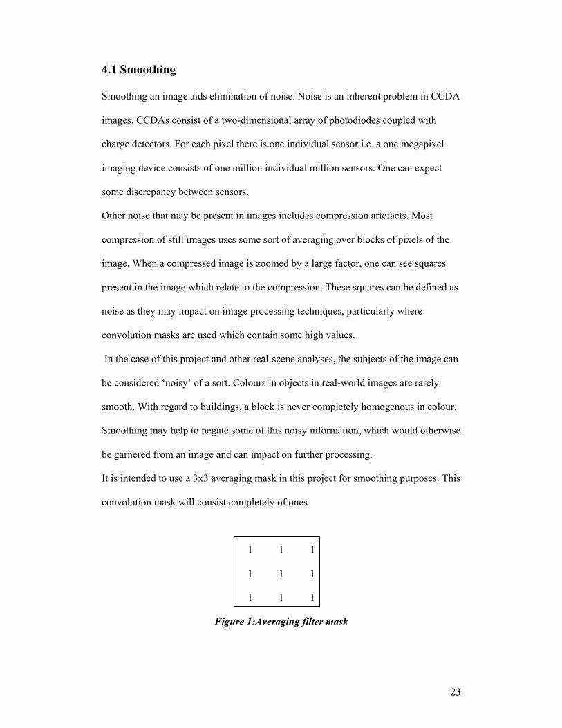
It is intended to use a 3x3 averaging mask in this project for smoothing purposes. This
convolution mask will consist completely of ones.
1 1 1
1 1 1
1 1 1
Figure 1:Averaging filter mask
24
4.2 Edge Detection
Edge detection is a common image processing / computer vision method. An edge can
be defined as a position in an image where pixel values change abruptly. Edge
detection may be performed in one or more channels of an image. Sometimes
luminance of an image is the sole channel of edge detection. However edge detection
may be performed in several channels simultaneously. This will produce an edge map
showing edges that exist in any of the channels. In the RGB colour space, this is a
recommendable approach as colours, which are adjacent in the image and easily
distinguishable to the eye, can be the same in two channels and differ only in the
other.
There are several edge detection methods, which can be categorised as being first
derivative or second derivative edge detectors. Although edge detection in images
works in the discrete domain, these methods are similar to their continuous
equivalents. First derivative edge detection methods look for peaks in the differences
between values, whilst second derivative methods look for zero-crossings in the first
derivative. Typically both categories of edge detection are implemented using
convolution masks. There are several commonly used masks for both methods.
First derivative detectors may produce two types of information. The gradient of an
edge relates the size of the change in value. The orientation of an edge relates the
direction of the maximum change in value. Two masks are used in the process of first
derivative edge detection. One calculates the gradient in the x-direction, whilst the
other calculates the gradient in the y-direction. The masks are +/- 90 degree rotations
of each other. The gradient is equal to the hypotenuse produced from combining the
root of the squares of these orthogonal values. The orientation of the edge is an angle
25
calculated from the arctan of the dividend of the y-gradient over the x-gradient.
Orientation may be expressed in two different ways, as one of eight directions leading
to an adjacent pixel, or as an angle. Orientation can be a very useful source of
information in further processing of edge maps. First derivative edge masks include
the Roberts, Prewitt, Sobel and isotropic masks.
Second Derivative edge detectors possess some benefit over first derivative methods.
Although sensitive to noise, theoretically at least, edges form closed loops. The
laplacian is a standard second derivative function. In image processing the laplacian is
found to be extremely sensitive to noise, and is generally subjected to gaussian
smoothing first in a method referred to as the laplacian of gaussian edge detector.
Second Derivative methods do not result in accurate gradient measure.
Good edge detection is vital to this project as all further processing is performed on
edge pixels and groupings of such. It is intended to use the Canny edge detector,
which includes the extra steps of non-maxima suppression, to thin lines, and hysterisis
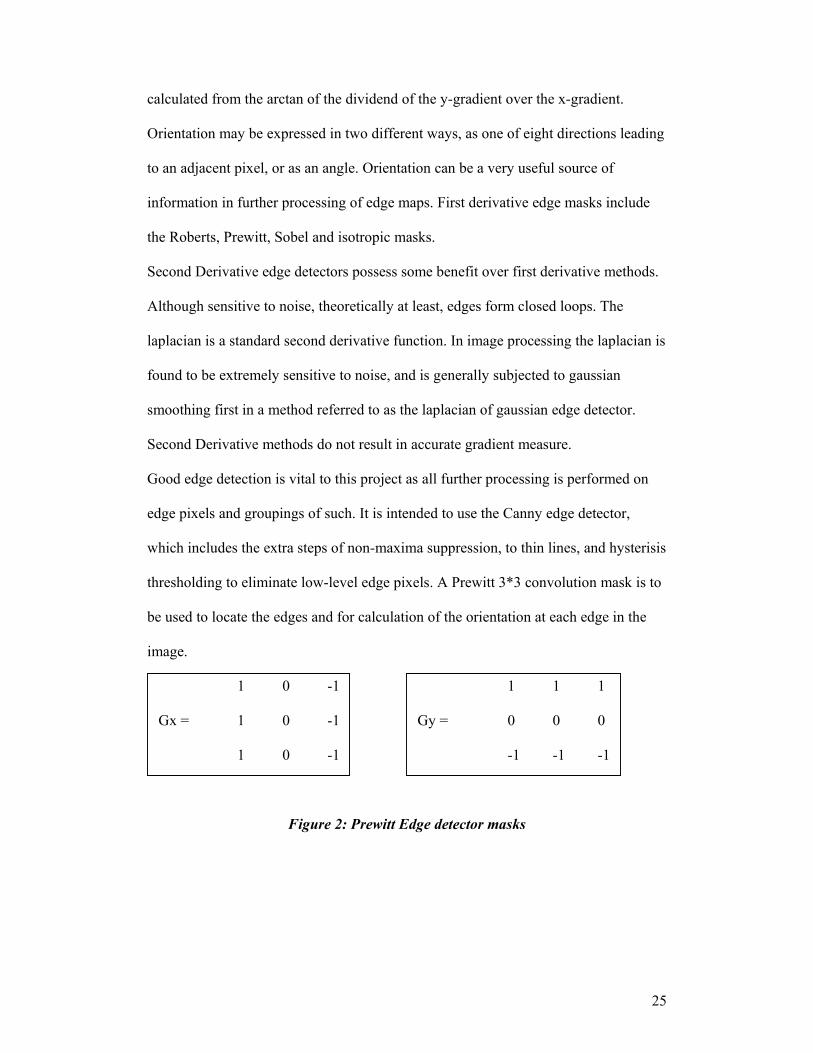
thresholding to eliminate low-level edge pixels. A Prewitt 3*3 convolution mask is to
be used to locate the edges and for calculation of the orientation at each edge in the
image.
1 0 -1 1 1 1
Gx = 1 0 -1 Gy = 0 0 0
1 0 -1 -1 -1 -1
Figure 2: Prewitt Edge detector masks
26
4.3 Non maxima suppression
Non-maxima suppression is a method used for thinning edges produced from first
derivative convolution masks. Edges are often not single pixel in width, a feature
which left alone would impact on further processing such as border detection.
Non-maxima suppression only keeps local maxima eliminating other edge pixels.
This is performed by comparing the gradient of each edge against each edge pixel
which is adjacent to it, and lies across it’s orientation.
As mentioned earlier, orientation may be defined in two distinct ways. As a direction,
pointing towards the adjacent pixel nearest to it’s orientation, or as an angle. Non-
maxima suppression may also be performed in two ways, depending on the format of
the orientation information.
If the orientation is described as one of eight directions, the two pixels, which lie
adjacent to the original edge pixel in question, and which lie across the orientation of
that pixel are selected. These pixels then have their gradient pixel values compared
against the gradient of the origin edge pixel. If the gradient of either of these pixels is
greater than the gradient at the origin pixel, the origin pixel is eliminated from the
edge map.
Alternatively if the orientation of the edge pixel is described as an angle it is possible
to perform the same method but to use the gradient values at sub-pixel points, which
lie directly across the orientation. The gradient at these sub-pixels can be calculated
from the gradient and distance of the edge pixels, which lie nearest to the subpixel.
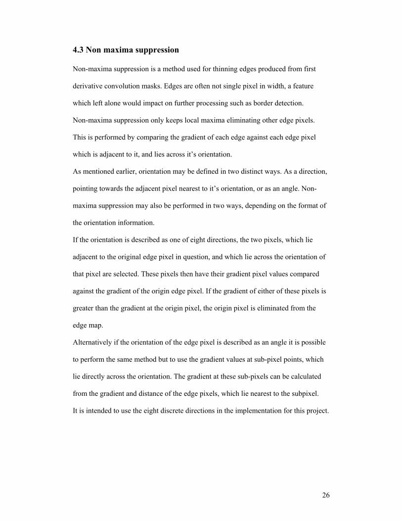
It is intended to use the eight discrete directions in the implementation for this project.
27
4.4 Hysterisis Thresholding
Thresholding is a simple method used to eliminate pixels from an image. A threshold
value is supplied. All pixels with a value above this threshold are kept, whilst values
below the threshold are eliminated. This can also be operated in reverse, keeping
pixels that lie below a threshold value.
Hysterisis thresholding is a method, which like non-maxima suppression, is part of the
Canny edge detector. In hysterisis thresholding, two threshold values are supplied. All
pixels with a gradient above the higher threshold value are kept and labelled as strong
candidates, whilst the pixels with a gradient below the lower value are eliminated.
The pixels with gradient value lying between the two thresholds are labelled as weak
candidates. The final step in hysterisis thresholding is to perform eight-connectivity
from each strong candidate pixel. All weak candidate pixels found during this step are
then labelled as strong candidates. When the eight-connectivity has been performed
from all strong pixels, including the strong pixels found during this step, all the
remaining weak candidate pixels are eliminated.
In this project it is intended to experiment with threshold values to determine if
optimum values for this type of application may be found across pictures, although
this is not expected to happen, and an alternative course of action will probably need
to be taken.
28
4.5 Edge Linking / Line segment Detection
Edge linking is the process of linking individual edge pixels into workable segments
or contours. It would be hoped that by linking edges in this way that borders can be
defined. A simple method of linking edge points is to check connectivity of all
adjacent edge points, known as eight-connectivity. Chain codes may be recorded,
relating the direction taken at each pixel from the starting pixel. When two new pixels
are found during a connectivity step at one pixel, one of them is added to the chain
and the other is labelled. When a chain is finished, or cannot grow any more, the same
process is repeated from each of the pixels labelled during the growth of the original
line.
An alternative method to using full eight connectivity is the A* algorithm. From each
pixel found, only three pixels are searched. The direction taken to find a pixel is
recorded. From this pixel, another pixel lying in the recorded direction is searched.
The two adjacent directions, laying either side of this recorded direction are also
searched
.
It is intended to use the A* algorithm in this implementation, as lines are the feature
of interest. When two or pixels are found at a search point it is intended to choose the
pixel of closest similarity, with respect to intensity, as the next pixel in a group
The A* algorithm can grow around corners. This means that groups of pixels found
during this search will contain branches at sharp angles to each other. As we are
looking for line segments, it is necessary to split these groups into component line
segments. It is expected to find squiggles, which ultimately are noise, as well.
29
Recursive splitting is to be performed on all groups found until each group is broken
down into component line segments and / or loose pixels. In the method of recursive
splitting, each group is defined as a line segment defined by the endpoints of the
group. At every point in the group, the deviation from this line segment is calculated.
If the deviation of any pixels is above an acceptable tolerance, the group will be split.
This splitting will occur at the point of maximum deviation from the line segment.
The same process is performed using the start point of the original line segment and
the point of maximum deviation as the ends of the line. This is performed recursively
until a line segment is found, or alternatively, until three or less pixels are left, in
which case they are considered loose pixels. When a line segment is found the start
point for the recursion moves to the previous point of maximum deviation, which is
the endpoint of the line segment found. This method is performed until all groups of
pixels in the image are classified as belonging to a line segment or a loose pixel.
A merging algorithm will then be applied which will attempt to merge back line
segments, which might have been split incorrectly, or were not completed due to a
missing edge pixel – a form of noise. At the end of each line segment, a local search
will be performed for other line segments, of similar angle. When found, these shall
be tested for line segment status by joining the two segments as one in a buffer
segment. This line segment will be checked for the maximum deviation from a line
drawn between it’s end points. If this maximum deviation is below a defined value,
the line segments will be discarded from the vector of segments, and the buffer
segment will be added to the segments vector. Otherwise the buffer segment will be
discarded. Different search shapes will be used depending on the slope, or angle of the
line from which the search is being performed.
30
4.6 Collinearity Detection
Collinearity detection between line segments will be performed as an alternative to
the Hough Transform. In this way salient line features will be determined, similar to
[15]. Each line segment will be defined by it’s start and end points, allowing the
slope, or the angle of the line to be determined, as well as the intercept with the y-
axis. To avoid comparing all line segments against each other for collinearity status,
line segments will be extended to the limits of image. During this extension, any other
line segments found at pixels of, or, nearest pixels to, this extended line will be
compared against the extended line for angle value. If the angles are relatively similar,
the two line segments will be joined as one, and redefined by the two furthest
endpoints. This new segment will be tested for line segment status, by the application
of deviation testing similar to the test performed for testing whether line segments
might merge. If this test is passed, a line shall be set up consisting of the segments.
Any further segments found to be collinear with the original will be added to this line.

31
4.7 Line Clustering
Clustering is a method of grouping objects according to similarity. A common method
of clustering is MacQueen K-means clustering. The K refers to the amount of cluster
to be gathered from the clustering process. K needs to be determined beforehand. This
can be a programmed constant or user input, depending on the program. Alternatively
a gaussian mixtures analysis may be performed to determine the amount of clusters
present in a sample, prior to k-means clustering.
Initial values are picked for the cluster centers. These values may be asserted in the
program or randomly picked, or also in the case of using a gaussian mixture analysis,
ascertained from the content of the sample. For each individual value in the sample, a
measure is then made to each of the cluster centres. This may be performed in many
dimensions, where appropriate metrics are predetermined. The value is then assigned
to the nearest cluster. At the end of this pass each cluster centre is calculated as the
mean (or median in k-medoid analysis) of the cluster. This process is repeated until
finally there is no change between passes.
For the purpose of this project, which is intended as a demonstration, all clustering
will be K-means, with K determined in the program. Clustering will be performed on
line segments, and will be performed on the angles and orientations of the lines.
The clustering of angles will be performed to allow vanishing point detection to be
carried out separately for each vanishing point. Only lines in a cluster related to a
particular vanishing point will be considered in the calculation of that vanishing point,
This is prerequisite for the vanishing point detection algorithm being used, as it only
allows for the detection of one vanishing point.
32
Orientation clustering will be performed to help prevent erroneous selection of line
segments during the collinearity detection process. Two adjacent, parallel edge line
segments will typically have opposite orientations.
4.8 Vanishing Point Detection
Most images portray a perspective viewpoint of the objects within. In many cases it is
necessary to rectify this perspective viewpoint, such as when pattern recognition with
a spatial element is required. Size and depth estimation of an object also require
similar treatment. The vanishing points relate information about the orientation of the
camera to an object in the scene.
As vanishing point detection was discussed in the background section, no further
discussion will take place here. It is intended to implement the vanishing point
detection algorithm described in [18]. The Hough Transform will not be implemented
in this project. However, for the purpose of experimentation with this method, all
lines found will be determined in a polar space.
Lines, which are eliminated during the search for the vanishing point, will be
eliminated from the image, and from further considerations. This is the first
elimination of any pixels that will have taken place since the hysterisis thresholding
stage
4.9 Perceptual Grouping
Perceptual Grouping is described in the background section. In this implementation,
only line segments that lie on lines, which are not eliminated during the vanishing
point detection stage, are considered for the perceptual grouping stage, as these can be
seen to relate to the important features in the building.

33
Chapter 5 : Implementation
In this section, reference will be made to sections of the design, in which problems
were encountered; indicating attempts to find solutions, and the reasoning behind the
various attempted solutions.
Figure 3: Original Image
5.1 Edge Detection & Non-maxima suppression
The first step taken was to smooth the image. This was done originally with the 3x3
window as indicated in the algorithm implementation. After implementing the 2-
window prewitt edge detector on this smoothed image ( see fig for gradient map and
fig for orientation map ), non-maxima suppression was performed using the eight
discrete directions. Several problems were noticed with this implementation. Firstly,
lines that were perpendicular or parallel to the borders of the image were seen to jump

34
from one column to the next at certain points. Other points were seen to disappear.
However neither of these problems rendered the implementation unworkable. When
using images with lines approaching 45 degrees to any of the image borders, as may
often happen in a perspective image, lines which were obvious in the image such as
window pane/ window sill borders were seen to disappear, becoming, at best,
perforated lines, which under subsequent border detection vanished without trace.
Figure 4: Smoothed Image
The hypothesis was formulated that the non-maxima suppression was suffering from
discretisation problems, causing adjacent pixels in the perceived line to have different
orientation directions to their neighbours. Whilst one original edge pixel might check
it’s value against those of two pixels lying solely in either the row or column of the
original edge pixel, a neighbour pixel might perform the same checking across a
35
diagonal, even though the actual orientation difference might be minimal.
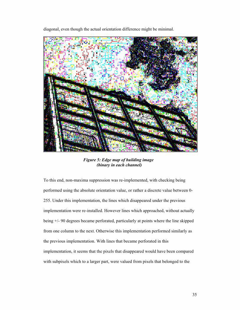
Figure 5: Edge map of building image (binary in each channel)
To this end, non-maxima suppression was re-implemented, with checking being
performed using the absolute orientation value, or rather a discrete value between 0-
255. Under this implementation, the lines which disappeared under the previous
implementation were re-installed. However lines which approached, without actually
being +/- 90 degrees became perforated, particularly at points where the line skipped
from one column to the next. Otherwise this implementation performed similarly as
the previous implementation. With lines that became perforated in this
implementation, it seems that the pixels that disappeared would have been compared
with subpixels which to a larger part, were valued from pixels that belonged to the
36
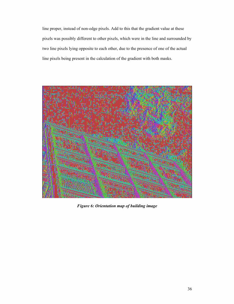
line proper, instead of non-edge pixels. Add to this that the gradient value at these
pixels was possibly different to other pixels, which were in the line and surrounded by
two line pixels lying opposite to each other, due to the presence of one of the actual
line pixels being present in the calculation of the gradient with both masks.
Figure 6: Orientation map of building image
37
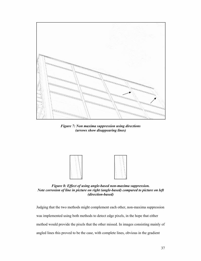
Figure 7: Non maxima suppression using directions (arrows show disappearing lines)
Figure 8: Effect of using angle-based non-maxima suppression. Note corrosion of line in picture on right (angle-based) compared to picture on left
(direction-based)
Judging that the two methods might complement each other, non-maxima suppression
was implemented using both methods to detect edge pixels, in the hope that either
method would provide the pixels that the other missed. In images consisting mainly of
angled lines this proved to be the case, with complete lines, obvious in the gradient
38
image, which had been compromised by the non-maxima suppression becoming
complete. However a problem was detected with lines, which were parallel to either
of the axes. In these lines the edge was complete. However there were individual
pixels jutting out from the line on a common but non-regular basis. Again in border
detection these had potential to cause problems.
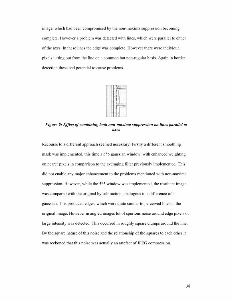
Figure 9: Effect of combining both non-maxima suppression on lines parallel to axes
Recourse to a different approach seemed necessary. Firstly a different smoothing
mask was implemented, this time a 5*5 gaussian window, with enhanced weighting
on nearer pixels in comparison to the averaging filter previously implemented. This
did not enable any major enhancement to the problems mentioned with non-maxima
suppression. However, while the 5*5 window was implemented, the resultant image
was compared with the original by subtraction, analogous to a difference of a
gaussian. This produced edges, which were quite similar to perceived lines in the
original image. However in angled images lot of spurious noise around edge pixels of
large intensity was detected. This occurred in roughly square clumps around the line.
By the square nature of this noise and the relationship of the squares to each other it
was reckoned that this noise was actually an artefact of JPEG compression.
39
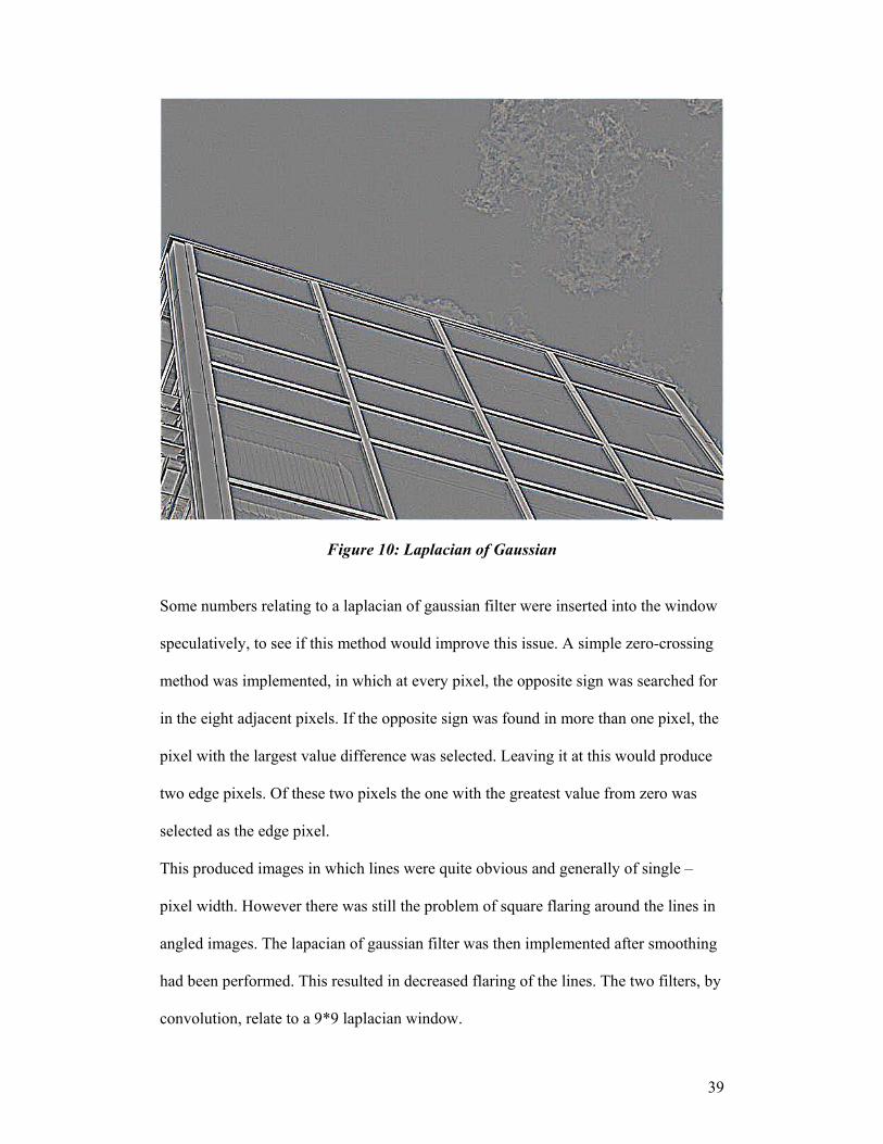
Figure 10: Laplacian of Gaussian
Some numbers relating to a laplacian of gaussian filter were inserted into the window
speculatively, to see if this method would improve this issue. A simple zero-crossing
method was implemented, in which at every pixel, the opposite sign was searched for
in the eight adjacent pixels. If the opposite sign was found in more than one pixel, the
pixel with the largest value difference was selected. Leaving it at this would produce
two edge pixels. Of these two pixels the one with the greatest value from zero was
selected as the edge pixel.
This produced images in which lines were quite obvious and generally of single –
pixel width. However there was still the problem of square flaring around the lines in
angled images. The lapacian of gaussian filter was then implemented after smoothing
had been performed. This resulted in decreased flaring of the lines. The two filters, by
convolution, relate to a 9*9 laplacian window.
40
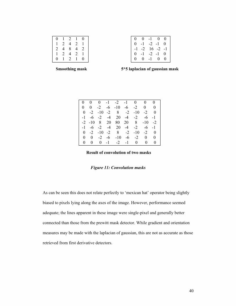
0 1 2 1 0 0 0 -1 0 0 1 2 4 2 1 0 -1 -2 -1 0 2 4 8 4 2 -1 -2 16 -2 -1 1 2 4 2 1 0 -1 -2 -1 0 0 1 2 1 0 0 0 -1 0 0
Smoothing mask 5*5 laplacian of gaussian mask
0 0 0 -1 -2 -1 0 0 0 0 0 -2 -6 -10 -6 -2 0 0 0 -2 -10 -2 8 -2 -10 -2 0 -1 -6 -2 -4 20 -4 -2 -6 -1 -2 -10 8 20 80 20 8 -10 -2 -1 -6 -2 -4 20 -4 -2 -6 -1 0 -2 -10 -2 8 -2 -10 -2 0 0 0 -2 -6 -10 -6 -2 0 0 0 0 0 -1 -2 -1 0 0 0
Result of convolution of two masks
Figure 11: Convolution masks
As can be seen this does not relate perfectly to ‘mexican hat’ operator being slightly
biased to pixels lying along the axes of the image. However, performance seemed
adequate; the lines apparent in these image were single-pixel and generally better
connected than those from the prewitt mask detector. While gradient and orientation
measures may be made with the laplacian of gaussian, this are not as accurate as those
retrieved from first derivative detectors.
41
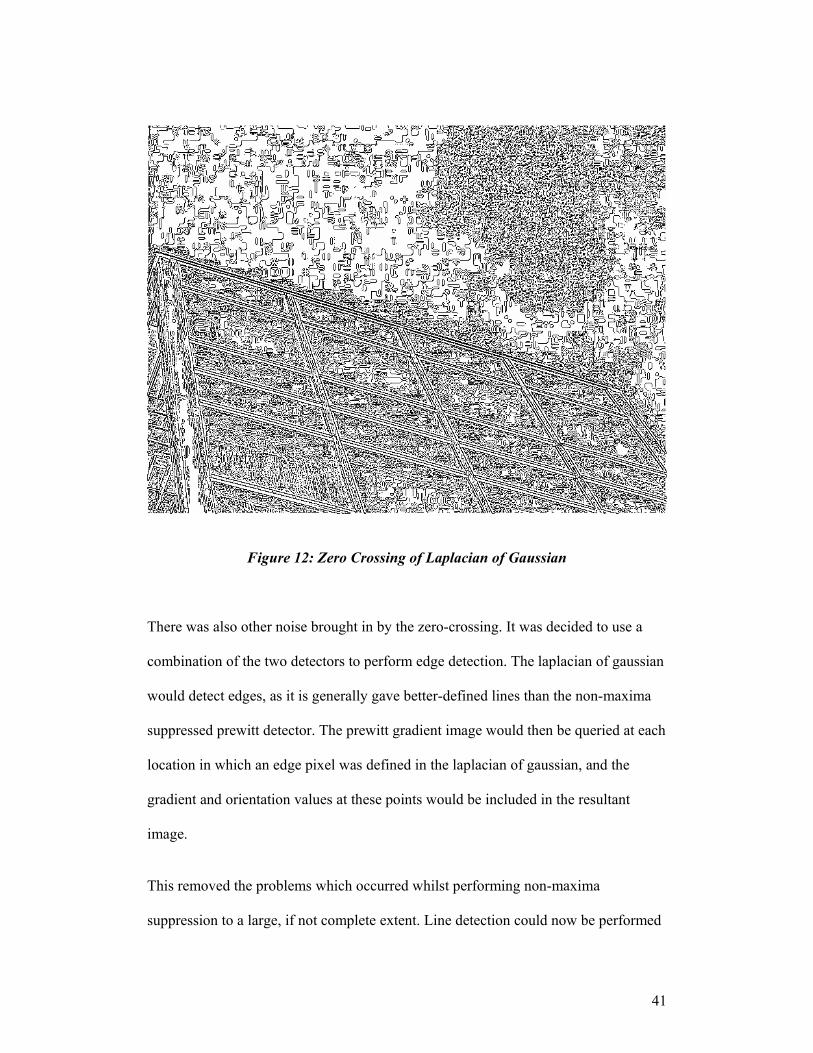
Figure 12: Zero Crossing of Laplacian of Gaussian There was also other noise brought in by the zero-crossing. It was decided to use a
combination of the two detectors to perform edge detection. The laplacian of gaussian
would detect edges, as it is generally gave better-defined lines than the non-maxima
suppressed prewitt detector. The prewitt gradient image would then be queried at each
location in which an edge pixel was defined in the laplacian of gaussian, and the
gradient and orientation values at these points would be included in the resultant
image.
This removed the problems which occurred whilst performing non-maxima
suppression to a large, if not complete extent. Line detection could now be performed
42
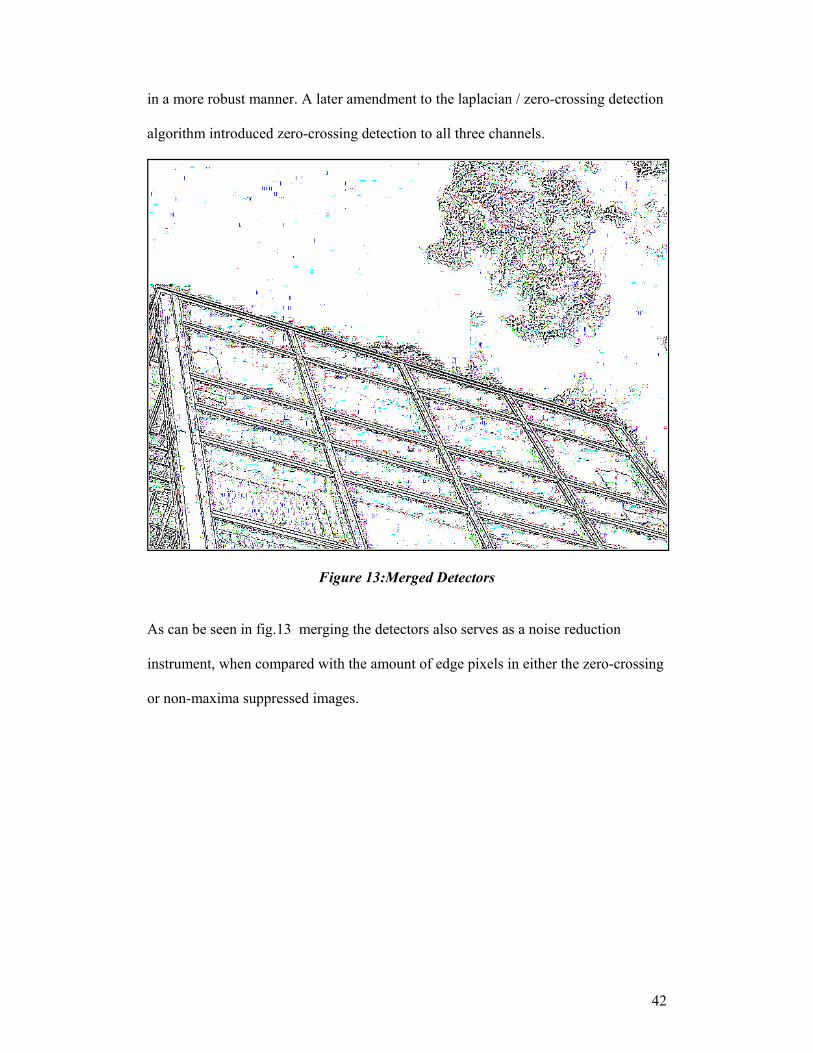
in a more robust manner. A later amendment to the laplacian / zero-crossing detection
algorithm introduced zero-crossing detection to all three channels.
Figure 13:Merged Detectors
As can be seen in fig.13 merging the detectors also serves as a noise reduction
instrument, when compared with the amount of edge pixels in either the zero-crossing
or non-maxima suppressed images.
43
5.2 Adaptive Hysterisis Thresholding
One problem with the resultant image, however, was the large amount of edge pixels
present. Up to this stage all edge pixels had been kept. Due to lighting and shading,
gradient values across an otherwise consistent line may change.
Simple thresholding was seen to remove some of these potentially important pixels.
For automation purposes, the definition of thresholds was seen to be a tricky issue.
The selection of two optimum values was not possible. The selection of two
reasonable thresholds, also, was seen to be tricky, due to the varying nature of
buildings and their features. It seemed reasonable to define the thresholds for
hysterisis thresholding as a function of the values of the edge pixels therein.
A histogram of the pixel intensities was performed. The quarter of the pixels, which
were most intense, were marked as strong; the quarter of least intense pixels were
eliminated from the image. From each of the strong pixels a recursive eight-
connectivity was performed, which stopped only when no more edge pixels were
found. Any pixels found during the course of the connectivity searches were kept in
the image. This included pixels which belonged to the middle half of the intensity
histogram, but none of the weaker ones. Any middle-value pixels which did not
connect to a strong point were now also eliminated from the image.
This method worked well on images of a viewpoint quite close to buildings, in which
features were large, eliminating a lot of pixels. In images taken further from an image,
whilst the requisite features were still maintained a lot of other points were also kept.
This would increase the processing needed in border detection for these images.
Possibly the premium solution might be a clustering step, for elimination of edge

44
pixels. One could possibly include the strongest pixel which a candidate pixel can
connect with, as well as the value of that candidate pixel, as attributes in this
clustering method.
Figure 14: Thresholded Edge Map after Adaptive Hysterisis
45
5.3 Edge Linking
First attempt considered recursive eight-connectivity on pixels found followed by
recursive splitting. While this was not the intended step, it was attempted due to ease
of implementation, and as a check of the efficiency of the recursive splitting
implementation.
When several edge pixels were found in an eight-connectivity step from an edge pixel
the one most similar in intensity was included in the group. At each point in the
growing the chaincode, relating the direction taken, was recorded. When the group
was finished growing the start and endpoints of the group were used to try to define
the group as a line segment. The considered line segment was defined by the angle
between these points. The deviation from this imaginary line was measured at each
edge point in the connected group. This was calculated by measuring the slope and
the length from the start point to the point in question. The angle between the ‘line
segment’ and this line was calculated by subtraction and the deviation from the line
determined as the sin of this angle by the length of the line from the start point to the
point in question.
One problem with this method was that small groups (less than roughly twelve pixels)
were often considered to be line segments when they were actually squiggles, which
could be seen to waver around a line drawn from the start to end pixels. These were
eliminated by considering the amount of chaincodes in the group, and comparing the
maximum deviation in a line segment against the amount of pixels in the group, for
small groups.
46
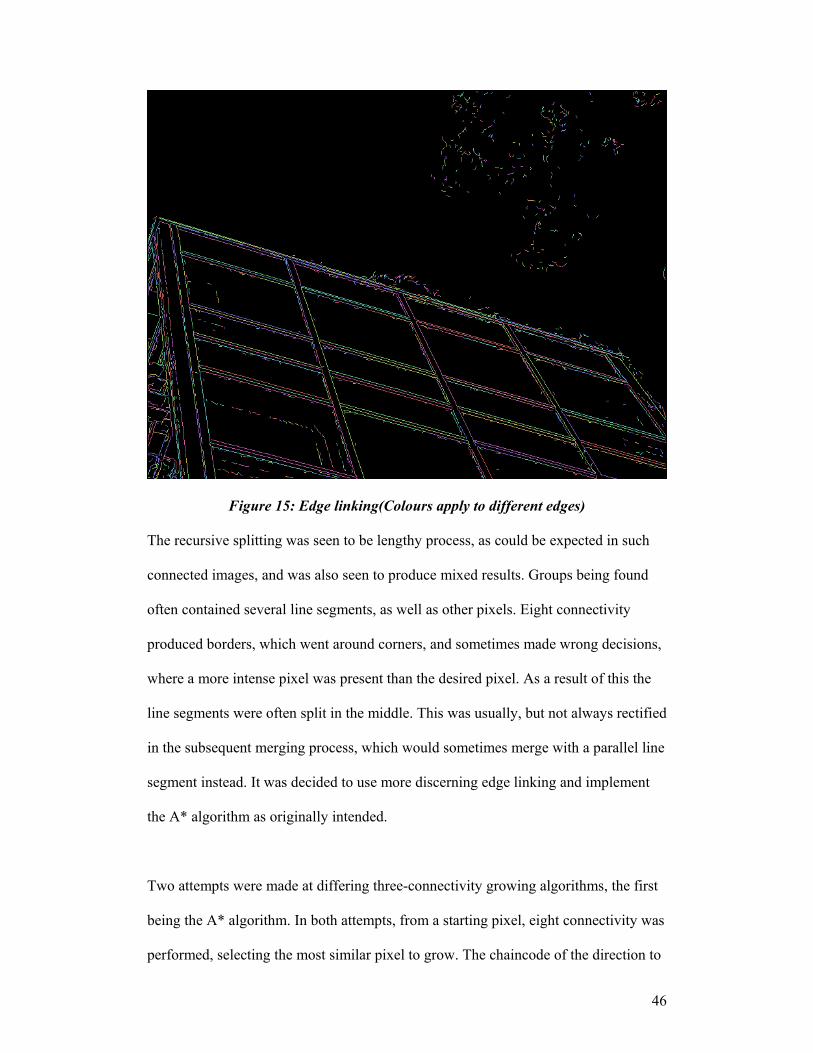
Figure 15: Edge linking(Colours apply to different edges) The recursive splitting was seen to be lengthy process, as could be expected in such
connected images, and was also seen to produce mixed results. Groups being found
often contained several line segments, as well as other pixels. Eight connectivity
produced borders, which went around corners, and sometimes made wrong decisions,
where a more intense pixel was present than the desired pixel. As a result of this the
line segments were often split in the middle. This was usually, but not always rectified
in the subsequent merging process, which would sometimes merge with a parallel line
segment instead. It was decided to use more discerning edge linking and implement
the A* algorithm as originally intended.
Two attempts were made at differing three-connectivity growing algorithms, the first
being the A* algorithm. In both attempts, from a starting pixel, eight connectivity was
performed, selecting the most similar pixel to grow. The chaincode of the direction to

47
this pixel was recorded, and from the new pixel, pixels in this central direction and the
immediately adjacent directions were checked for connectivity; again, in the case of
more than one candidate pixel being found, the most similar pixel being added. The
direction taken to a pixel was considered the central direction at that pixel. This
continued until no candidate pixels were found at a point.
The A* algorithm caused lines to split where there was one point, which deviated
from the line. However performance was relatively robust, and a decrease in
performance time was noticeable (if not recorded) due to the decreased search at each
point, and decreased recursive splitting required.
As it was decided to concentrate on straight lines in building images, a similar three
connectivity was implemented which maintained a constant central direction search
throughout the line growth. This central direction was defined as the direction taken in
the original eight connectivity. This was found to work well. However in the case of
growing curves it would be necessary to revert to the A* algorithm.
The next step was to perform merging of line segments in the image into larger line
segments. A first attempt compared all line segments to each other. If the difference
between their angles was below a certain threshold, further comparison was made.
Both sets of endpoints were checked against each other for the separation between
them. If a separation below a threshold was found, the angle between the midpoints s
of the two lines was calculated and compared to the angles of the line segments in
question. In this way it was hoped to eliminate merging two lines were there was a
better candidate line for merging. The pixels of each line were added together and line
segment classification similar to that performed during recursion was performed,
48
albeit with a slightly larger maximum deviance threshold. This algorithm was found
to be not very successful. Lines parallel to the best possible segment for merging, in a
given case, were sometimes chosen for merging when they were close. Also a lot of
lines, which could have been merged, were not merged at all. There were also cases
where edge pixels had been defined as loose lay between line segments that otherwise
might have been merged. Another hypothesis for the weakness of the previous
merging algorithm was the definition of angles of lines. As during the splitting stage
groups were split at points of maximum deviation, a lot of line segments had an
endpoint that was offset slightly from the real line. This could be seen as an error of
the imaging device, of the edge detection, or of the constraints of the splitting
algorithm. As the angle of the line segment was measured as the angle between the
endpoints, the accuracy of the angle measure is very dependent on having an endpoint
that represents the line, which is not necessarily the result, having performed line
splitting. Also, the algorithm was massively expensive in processing costs due to the
large amount of line segments present.
Before writing a second implementation of a merging algorithm, a linear regression
was performed on all line segments, allowing for a truer definition of the line
segment’s angle and intercept. Later, a further alteration was made to this
implementation, and lines were defined by their x and y mean values instead of their
y-intercept values, which was found to be slightly more accurate, especially with lines
which tended towards the vertical. As opposed to comparing all line segments to each
other for distance between endpoints and similarity of line angle, for performance
sakes, it was proposed to attempt a local search at the end of each line segment. In this
way loose pixels might also be found which might merge. Loose pixels which were
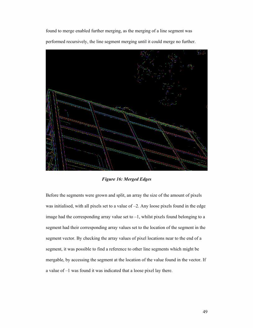
49
found to merge enabled further merging, as the merging of a line segment was
performed recursively, the line segment merging until it could merge no further.
Figure 16: Merged Edges
Before the segments were grown and split, an array the size of the amount of pixels
was initialised, with all pixels set to a value of –2. Any loose pixels found in the edge
image had the corresponding array value set to –1, whilst pixels found belonging to a
segment had their corresponding array values set to the location of the segment in the
segment vector. By checking the array values of pixel locations near to the end of a
segment, it was possible to find a reference to other line segments which might be
mergable, by accessing the segment at the location of the value found in the vector. If
a value of –1 was found it was indicated that a loose pixel lay there.
50
The segment found at this location in the vector could then have it’s angle compared
with the original line segment. If similar an attempt could be made to merge the lines.
In this implementation, a check to see if this new amalgamated pixel group referred to
a line segment was performed by adding the pixels of the lines together, furthest point
to furthest point and performing a linear regression on this group and checking that
the maximum value of deviation was below a low threshold.
This performed more successfully than the first attempt at merging and was massively
computationally cheaper. Further amendments to this algorithm considered similarity
of orientation as the factor of choice in pixel selection where several candidate pixels
were present. This was seen to improve on the use of intensity as the deciding factor.
Further again, and a combination of the two values, orientation and gradient intensity,
was used to decide the selection of the best pixel. Two probability ratings were given
to each pixel based on orientation and gradient intensity. These were then multiplied
to give an unnormalised probability for the pixel. To weight the rating closer to the
orientation, intensity was rated using a straight-line function, falling off equally for
each unit value whilst orientation was rated using a cosine function of the value
difference. This was seen to cause a large increase in the correlation between user-
observed selections and computer selections.
5.4 Collinearity
A similar approach was then taken to finding collinearity between line segments after
merging. A local search was performed by extending the line segment into a line that
traversed the image fully, by using the parameters of the line segment. At every few
pixels this line was checked to see if it coincided with another line segment. The
pixels either side of the line were also checked. All line segments found were
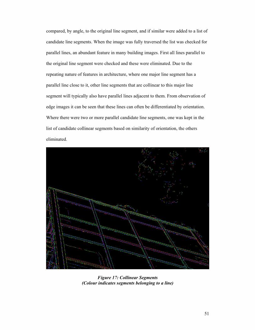
51
compared, by angle, to the original line segment, and if similar were added to a list of
candidate line segments. When the image was fully traversed the list was checked for
parallel lines, an abundant feature in many building images. First all lines parallel to
the original line segment were checked and these were eliminated. Due to the
repeating nature of features in architecture, where one major line segment has a
parallel line close to it, other line segments that are collinear to this major line
segment will typically also have parallel lines adjacent to them. From observation of
edge images it can be seen that these lines can often be differentiated by orientation.
Where there were two or more parallel candidate line segments, one was kept in the
list of candidate collinear segments based on similarity of orientation, the others
eliminated.
Figure 17: Collinear Segments (Colour indicates segments belonging to a line)
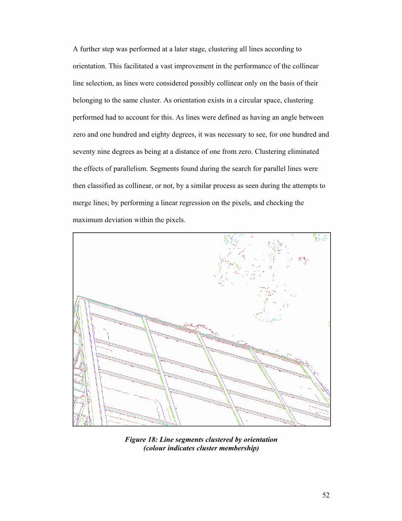
52
A further step was performed at a later stage, clustering all lines according to
orientation. This facilitated a vast improvement in the performance of the collinear
line selection, as lines were considered possibly collinear only on the basis of their
belonging to the same cluster. As orientation exists in a circular space, clustering
performed had to account for this. As lines were defined as having an angle between
zero and one hundred and eighty degrees, it was necessary to see, for one hundred and
seventy nine degrees as being at a distance of one from zero. Clustering eliminated
the effects of parallelism. Segments found during the search for parallel lines were
then classified as collinear, or not, by a similar process as seen during the attempts to
merge lines; by performing a linear regression on the pixels, and checking the
maximum deviation within the pixels.
Figure 18: Line segments clustered by orientation (colour indicates cluster membership)
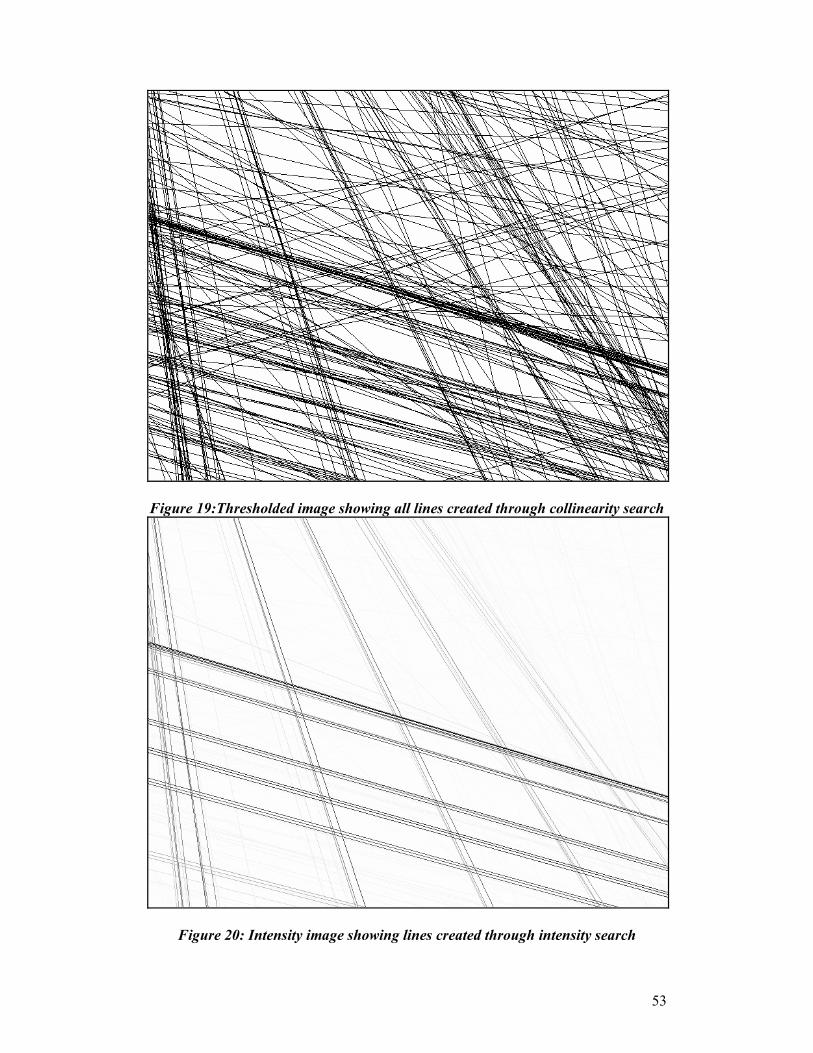
53
Figure 19:Thresholded image showing all lines created through collinearity search
Figure 20: Intensity image showing lines created through intensity search
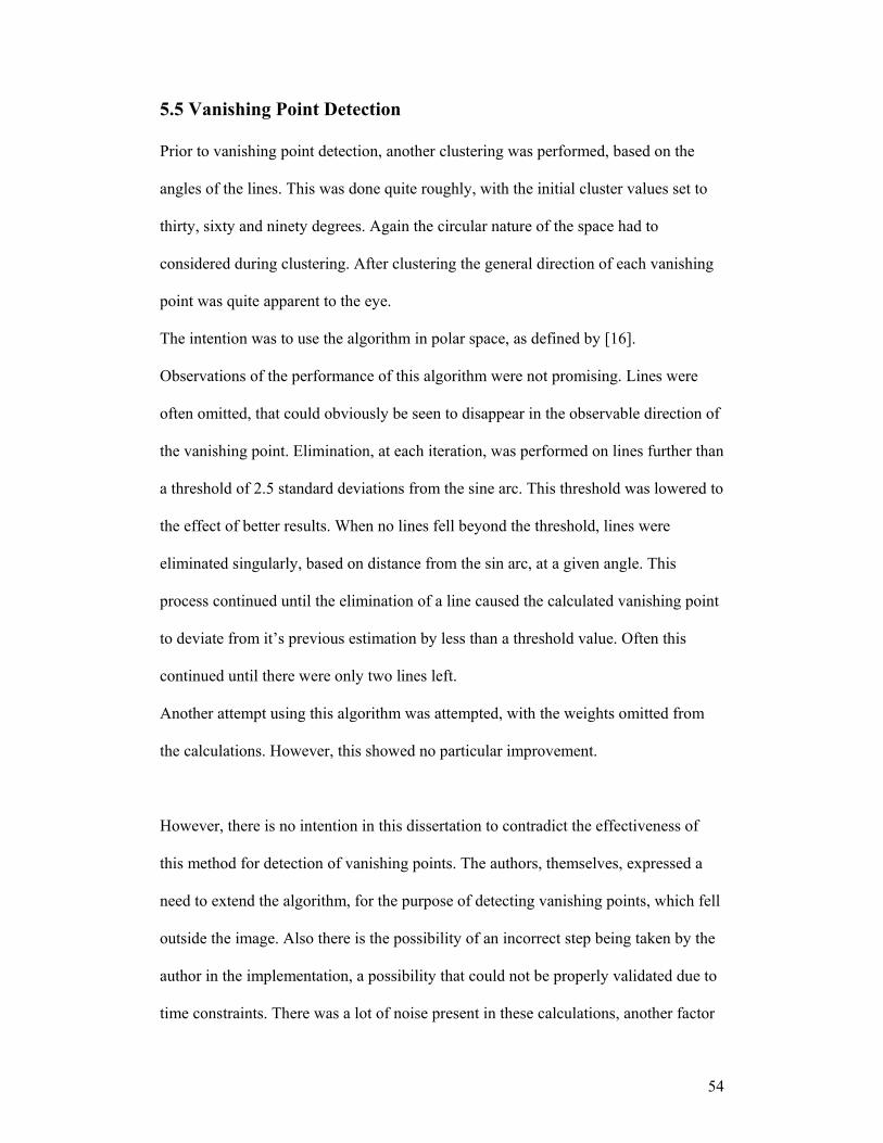
54
5.5 Vanishing Point Detection
Prior to vanishing point detection, another clustering was performed, based on the
angles of the lines. This was done quite roughly, with the initial cluster values set to
thirty, sixty and ninety degrees. Again the circular nature of the space had to
considered during clustering. After clustering the general direction of each vanishing
point was quite apparent to the eye.
The intention was to use the algorithm in polar space, as defined by [16].
Observations of the performance of this algorithm were not promising. Lines were
often omitted, that could obviously be seen to disappear in the observable direction of
the vanishing point. Elimination, at each iteration, was performed on lines further than
a threshold of 2.5 standard deviations from the sine arc. This threshold was lowered to
the effect of better results. When no lines fell beyond the threshold, lines were
eliminated singularly, based on distance from the sin arc, at a given angle. This
process continued until the elimination of a line caused the calculated vanishing point
to deviate from it’s previous estimation by less than a threshold value. Often this
continued until there were only two lines left.
Another attempt using this algorithm was attempted, with the weights omitted from
the calculations. However, this showed no particular improvement.
However, there is no intention in this dissertation to contradict the effectiveness of
this method for detection of vanishing points. The authors, themselves, expressed a
need to extend the algorithm, for the purpose of detecting vanishing points, which fell
outside the image. Also there is the possibility of an incorrect step being taken by the
author in the implementation, a possibility that could not be properly validated due to
time constraints. There was a lot of noise present in these calculations, another factor
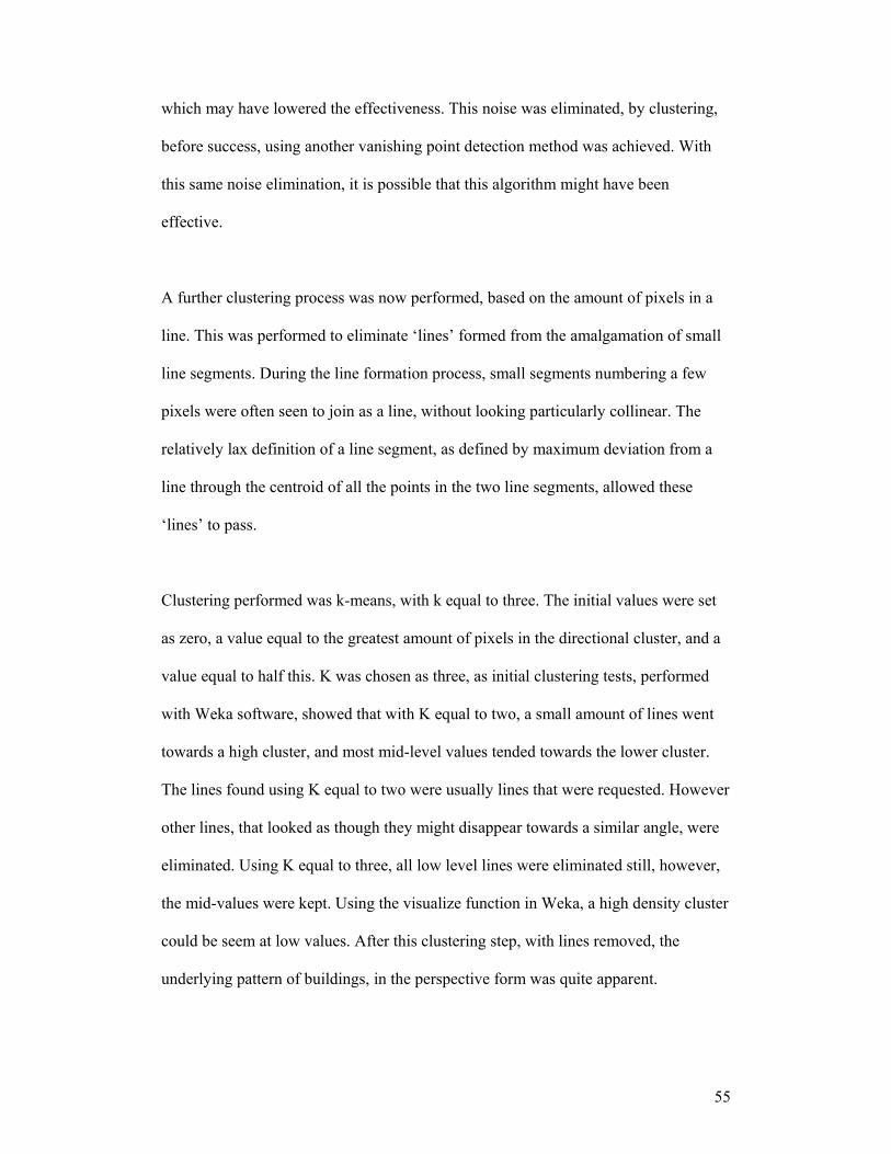
55
which may have lowered the effectiveness. This noise was eliminated, by clustering,
before success, using another vanishing point detection method was achieved. With
this same noise elimination, it is possible that this algorithm might have been
effective.
A further clustering process was now performed, based on the amount of pixels in a
line. This was performed to eliminate ‘lines’ formed from the amalgamation of small
line segments. During the line formation process, small segments numbering a few
pixels were often seen to join as a line, without looking particularly collinear. The
relatively lax definition of a line segment, as defined by maximum deviation from a
line through the centroid of all the points in the two line segments, allowed these
‘lines’ to pass.
Clustering performed was k-means, with k equal to three. The initial values were set
as zero, a value equal to the greatest amount of pixels in the directional cluster, and a
value equal to half this. K was chosen as three, as initial clustering tests, performed
with Weka software, showed that with K equal to two, a small amount of lines went
towards a high cluster, and most mid-level values tended towards the lower cluster.
The lines found using K equal to two were usually lines that were requested. However
other lines, that looked as though they might disappear towards a similar angle, were
eliminated. Using K equal to three, all low level lines were eliminated still, however,
the mid-values were kept. Using the visualize function in Weka, a high density cluster
could be seem at low values. After this clustering step, with lines removed, the
underlying pattern of buildings, in the perspective form was quite apparent.
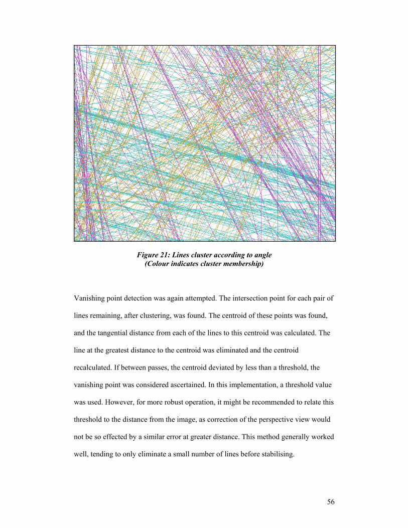
56
Figure 21: Lines cluster according to angle (Colour indicates cluster membership)
Vanishing point detection was again attempted. The intersection point for each pair of
lines remaining, after clustering, was found. The centroid of these points was found,
and the tangential distance from each of the lines to this centroid was calculated. The
line at the greatest distance to the centroid was eliminated and the centroid
recalculated. If between passes, the centroid deviated by less than a threshold, the
vanishing point was considered ascertained. In this implementation, a threshold value
was used. However, for more robust operation, it might be recommended to relate this
threshold to the distance from the image, as correction of the perspective view would
not be so effected by a similar error at greater distance. This method generally worked
well, tending to only eliminate a small number of lines before stabilising.

57
Figure 22: Line Clusters after further clustering by line weight (only shows two line clusters)
However, where only a small amount of a side of a building was visible, this detection
was seen to be erroneous. The clustering by angles step may produce a cluster, which
consists of lines, the majority of which may not actually belong to the plane for the
vanishing point detection is being performed. It might be recommended to perform
planar sectioning before this step. A simple implementation of this would consist of
clustering lines due to the location of their constituent line segments, relative to the
lines vanishing to the azimuth.
58
Figure 23: Lines going to vanishing point
Figure 24:Line Segments belonging to vanishing lines

59
Perceptual grouping in the form of a search for L-shapes consisting of junctions
caused by remaining line segments near junctions of lines which had not been
eliminated by the vanishing point detection. This worked as hoped.
60
Chapter 6 : Conclusions
Using computer vision techniques on buildings in an automatic fashion is a nontrivial
task, consisting of many potential pitfalls. However it may be a reasonable application
of these techniques. To build a fully automatic building recognition system would
require the inclusion of extra methodologies.
Some form of local to global colour clustering may need to be performed, to
understand better the nature of the image, including the perception of negative space.
An implementation of a more robust border detection algorithm is a must especially if
dealing with brick buildings. Texture analysis might also be added.
Trying to recognise more complicated buildings with many planes would introduce
more challenges. A program attempting to do this would probably have to understand
the occlusion of faces of buildings by other faces of the same building, as well as by
other objects in the environment.
A lot of research, relevant to this sort of application, has been done by the
architectural photogrammetry community, in pursuit of the goal of modelling
buildings accurately for the purpose of Computer Aided Architectural Design
projects. The goal of these projects is to show a model of a new building, which has
been modelled in CAD, in it’s surrounding environment, which consists of buildings
for which no CAD model exists. However, most of this research has not been based
on the need for automation.
Automation of many of these methods would require a program, which would
probably need to infer some probability on the identification of complex buildings,
before further model-based processing.
61
Appendix A : References [1] Norbert Haala & Jan Bohm, “A multi-sensor system for positioning in urban environments”. ISPRS Journal of Photogrammetry & Remote Sensing 58 (2003) pp31-42 [2] Daniel Wagner, Dieter Schmalsteig, “First steps towards Handheld Augmented Reality” Proceedings of the seventh IEEE International Symposium on Wearable Computers [3] Qasim Iqbal & J.K Aggarwal, “Applying perceptual grouping to content-based image retrieval: Building Images”, Proceedings of the IEEE International Conference on Computer Vision and Pattern Recognition, June 23-26, Fort Collins, Colorado, USA pp42-48 [4] Qasim Iqbal & J.K Aggarwal “Retrieval by classification of images containing large manmade objects using perceptual grouping” Pattern Recognition 35(2002) pp1463-1479 [5] Xiang Sean Zhou, Yong Rui, Thomas S.Huang, “Water-filling: A novel way for image structural feature extraction”, http://research.microsoft.com/~yongrui/ipsicp99a.pdf [6] Yi Li & Linda G. Shapiro, “Consistent Line Clusters for building recognition in CBIR”, 16th International Conference on pattern recognition(ICPR ’02) Volume 3 [7] Wei Zhang & Jana Kosecka, “Experiments in Building Recognition”, http://cs.gmu.edu/~tr-admin/papers/GMU-CS-TR-2004-3.pdf [8] Norbert Haala, Jan Bohm, Martin Kada, “Processing of 3D building models for location aware applications”, International Archives on Photogrammetry and Remote Sensing Volume XXXIV pp157-162 [9] Jan Bohm, Norbert Haala, Peter Kapusy, “Automated Appearance-Based Building Detection in Terrestrial Images”, International Archives on Photogrammetry and Remote Sensing Volume XXXIV pp491-495 [10] David Lowe, “Object Recognition from local scale-invariant features”, Proceedings of the International Conference of ComputerVision ICCV pp 1150-1157

62
[11] Ismail Haritaoglu, “Infoscope: Link from real world to Digital Information Space”, Lecture Notes in Computer Science; Vol 2201 Proceedings of the 3rd international conference on Ubiquitous Computing [12] Xiangrong Chen & Alan L. Yuille “Detecting and reading text in Natural Scenes” Proceedings of the 2004 IEEE computer society on computer vision and pattern recognition Volume 2 pp366-373 [13] Keechul Jung, Kwang In Kim, Takeshi Kurata, Masakastu Kourogi, JungHyun Han, “Text Scanner with text detection technology on image sequences”, 16th International Conference n Pattern Recognition Volume , pp30473 [14] Wanji Mai, Gordon Dodds, Chris Tweed “A PDA-Based system for recognizing buildings from User-Supplied Images” Mobile and Ubiquitous Information Access Ws 2003, LNCS 2954 pp143-157 [15] Christopher Jaynes “View Alignment of Aerial and Terrestrial Imagery in Urban Environments” Integrated Spatial Databases’ 99 pp 3 – 19 [16] Virginio Cantoni, Luca Lombardi, Marco Portam Nicolas Sicard, “Vanishing Point Detection: Representation Analysis and New Approaches”, Proceedings of the 11th international Conference on Image Analysis and Processing [17] Frank A. van den Heuvel, “Reconstruction from a single architectural image from the MeyDenBaeur Archives”, ISPRS Journal for Photogrammetry and Remote Sensing (??) [18] Andrea Matessi & Luca Lombardi “Vanishing Point Detection in the Hough Transform” Lecture Notes in Computer Science, Vol. 1685 Proceedings of the 5th International Euro-Par Conference on Parallel Processing pp987 - 994 [19] W. Forstner & E.Gulch, “Automatic Orientation and Recognition in Highly Structured Scenes”, Videometrics V, Integrating Photogrammetric Techniques with Scene Analysis and Machine Vision III

63
[20] Frank A. van Der Heuvel, “Exterior Orientation using Coplanar Lines”, Proceedings of the 10th Scandinavian Conference on Image Analysis pp71-78 [21] John Krumm, Eric Horvitz, “Locadio: Inferring Motion and Location from WI-FI Signal Strengths”, First Annual International Conference on Mobile and Ubiquitous Systems: Networks and Services pp4-13
64
Appendix B : Framework Overview
Courtesy Of Colm Conroy 1 Information Eye
In Urban based Systems there is a need for location based information and services [5].
However location detection within a city with GPS [10] is often unreliable. We propose a
solution for providing urban based Systems with location based information and services
through the use of image processing to detect where a user is located, structuring geographical
information into a format which can be queried, and an ability to share data between agents.
To facilitate these research objectives a framework was defined providing the ability for a
mobile user to:
1. Capture photographic information which is reasoned with an image based technology
to form primitive shapes,
2. Query a Geographical Ontology (with buildings represented as shapes) to provide
location based knowledge and services,
3. And finally a service to allow the sharing of mappings between related Ontologies.
The project was split into these three specific areas with Ken O’Hanlon responsible for the
image based technology, while Yaou Li was responsible for the Geographical Ontology and
location service, and the author was responsible for the development of a service to provide
the sharing of mappings between ontologies. Our overall framework’s capabilities are
described in Section 1.1.1.
2 Overall Framework Overview
Figure 1 shows a diagram model of the whole project structure framework. The main
components are a mobile application with the ability to process photographic information into
shapes, a web service with the ability to query a Ontology with this shape information to find
the users location and to also provide location based services, and finally a peer to peer
service with the ability to provide updated Ontology Mappings to other corresponding
ontologies.
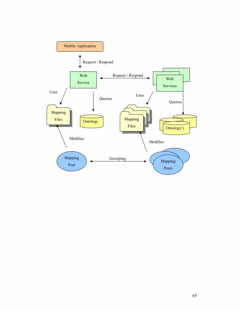
65
Request / Respond
Request / Respond
Uses Uses
Gossiping
Queries
Ontology Ontology’s
Mapping
Peer Mapping
Peers
Mapping
Files Mapping
Files
Web
Service Web
Services
Mobile Application
Queries
Modifies Modifies