building software systems at google and lessons learned · building software systems at google and...
TRANSCRIPT


Plan for Today
• Evolution of various systems at Google–computing hardware–core search systems–infrastructure software
• Techniques for building large-scale systems –decomposition into services–design patterns for performance & reliability
–Joint work with many, many people
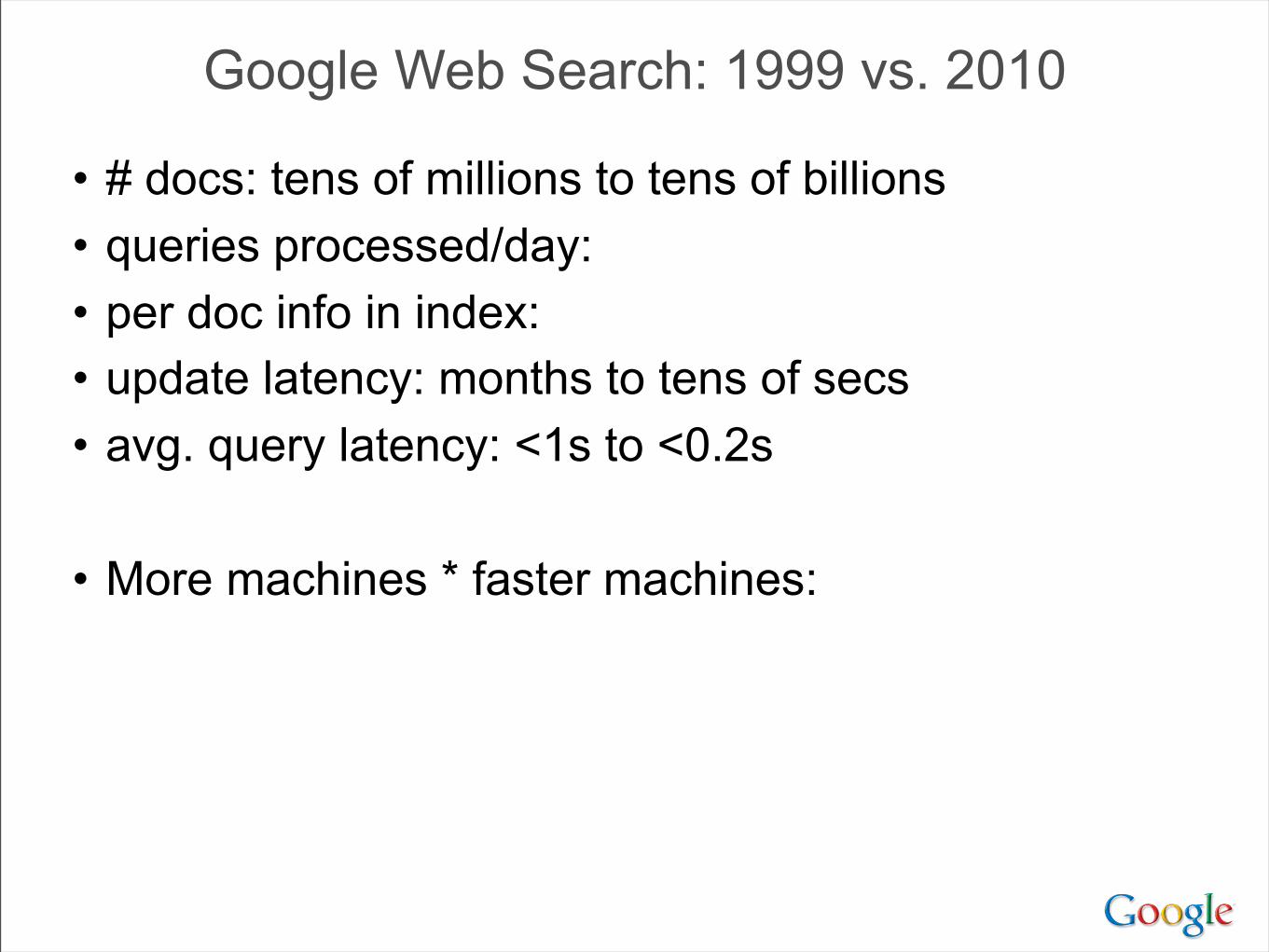
• # docs: tens of millions to tens of billions• queries processed/day:• per doc info in index: • update latency: months to tens of secs• avg. query latency: <1s to <0.2s
• More machines * faster machines:
Google Web Search: 1999 vs. 2010
• # docs: tens of millions to tens of billions• queries processed/day:• per doc info in index: • update latency: months to tens of secs• avg. query latency: <1s to <0.2s
• More machines * faster machines:
Google Web Search: 1999 vs. 2010
~1000X

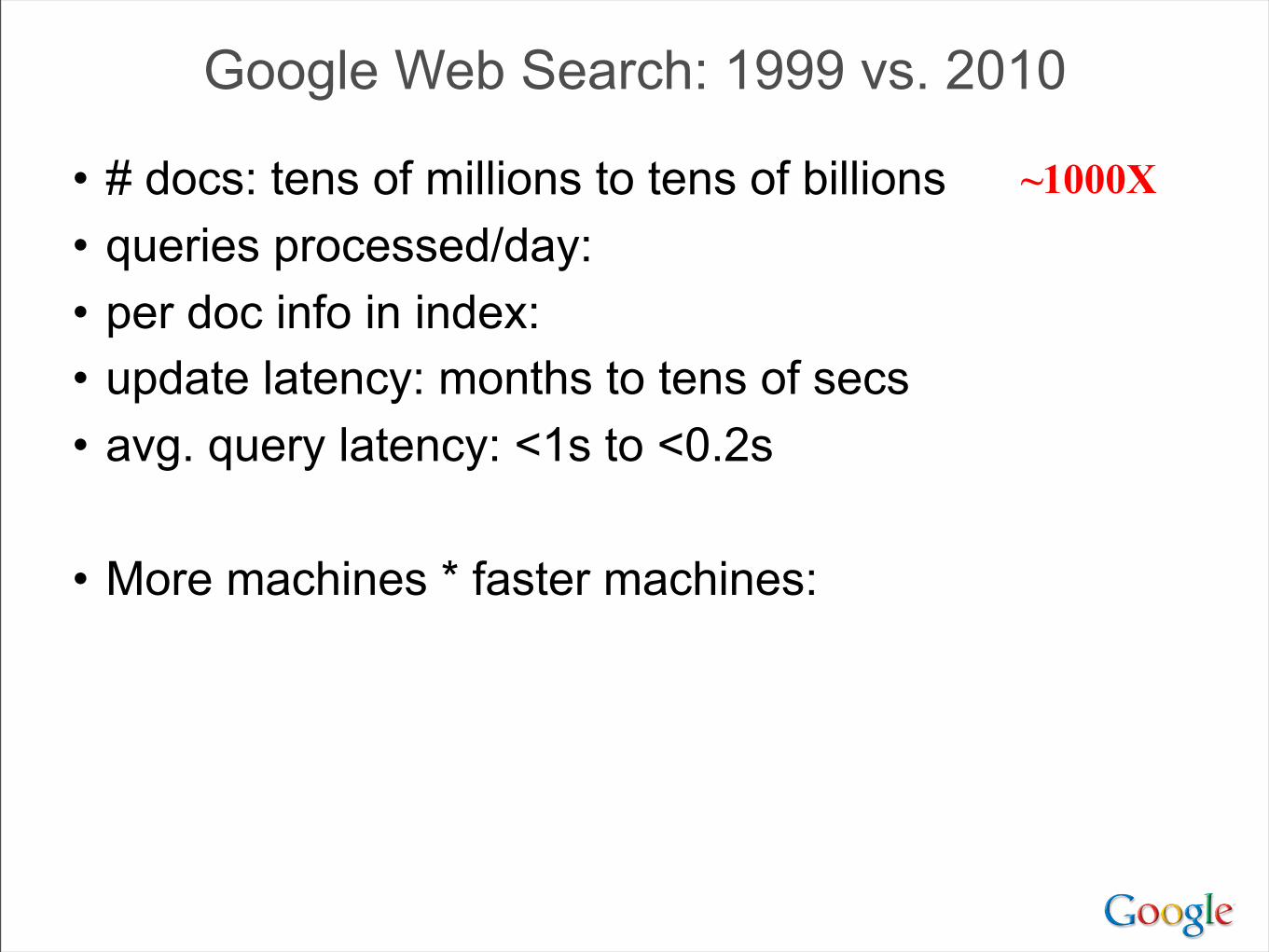
• # docs: tens of millions to tens of billions• queries processed/day:• per doc info in index: • update latency: months to tens of secs• avg. query latency: <1s to <0.2s
• More machines * faster machines:
Google Web Search: 1999 vs. 2010
~1000X~1000X
• # docs: tens of millions to tens of billions• queries processed/day:• per doc info in index: • update latency: months to tens of secs• avg. query latency: <1s to <0.2s
• More machines * faster machines:
Google Web Search: 1999 vs. 2010
~1000X
~3X~1000X

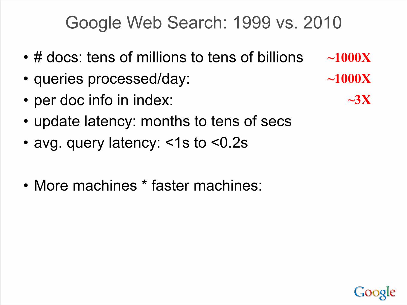
• # docs: tens of millions to tens of billions• queries processed/day:• per doc info in index: • update latency: months to tens of secs• avg. query latency: <1s to <0.2s
• More machines * faster machines:
Google Web Search: 1999 vs. 2010
~1000X
~3X~1000X
~50000X
• # docs: tens of millions to tens of billions• queries processed/day:• per doc info in index: • update latency: months to tens of secs• avg. query latency: <1s to <0.2s
• More machines * faster machines:
Google Web Search: 1999 vs. 2010
~1000X
~3X~1000X
~50000X
~5X

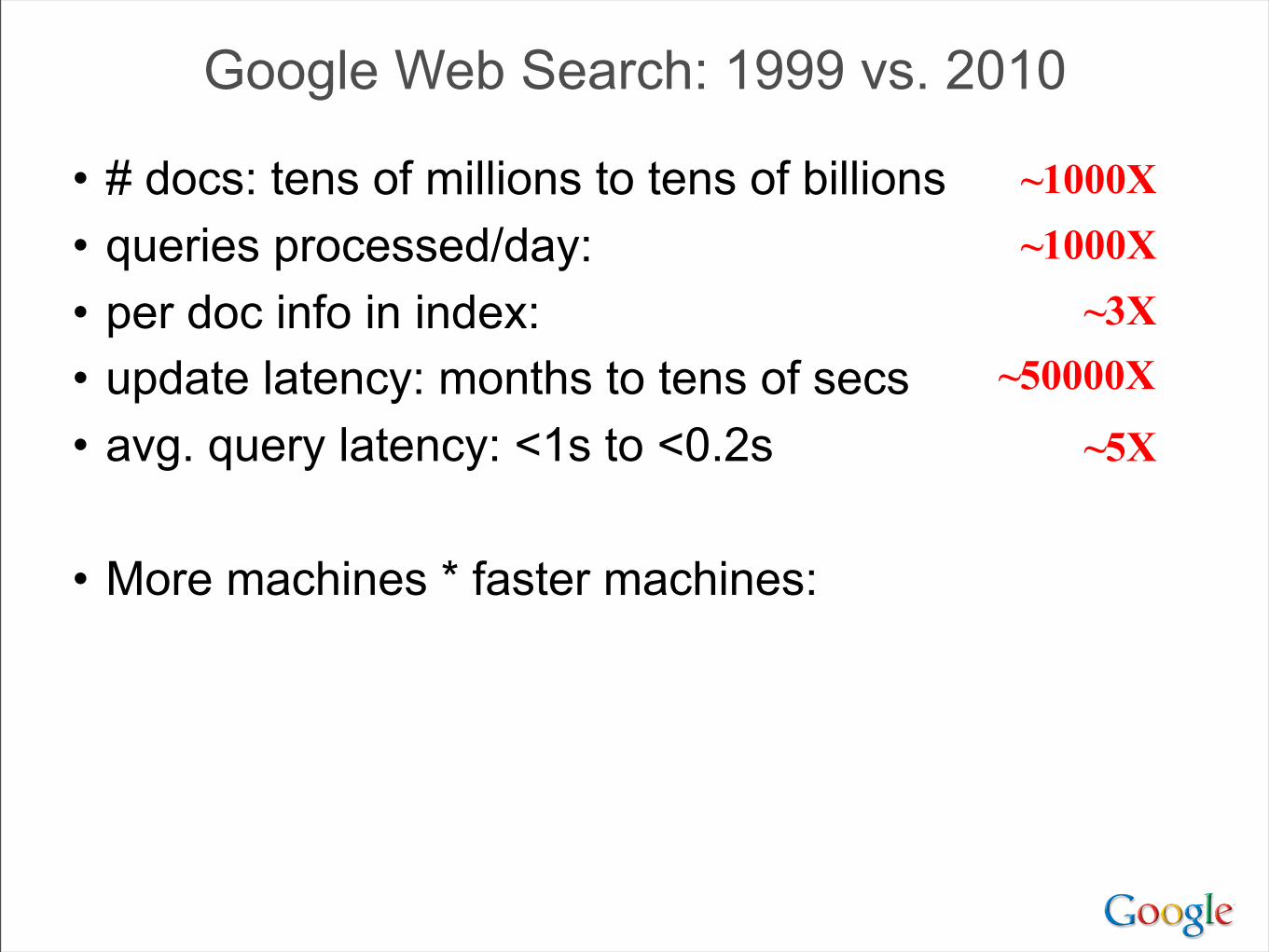
• # docs: tens of millions to tens of billions• queries processed/day:• per doc info in index: • update latency: months to tens of secs• avg. query latency: <1s to <0.2s
• More machines * faster machines:
Google Web Search: 1999 vs. 2010
~1000X
~3X~1000X
~50000X
~5X
~1000X
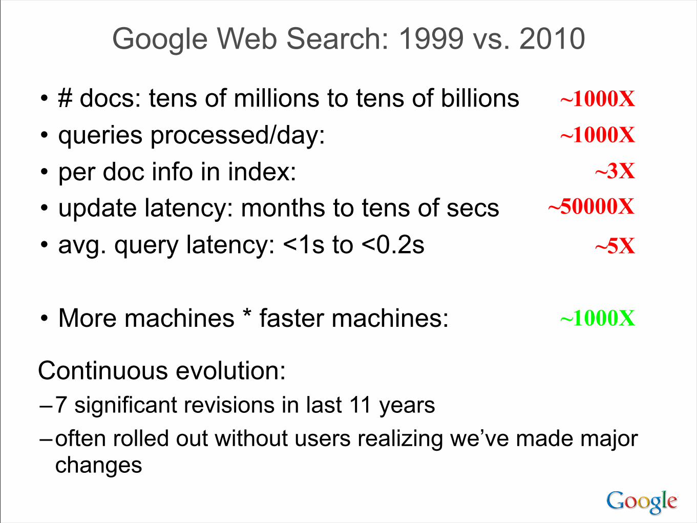
• # docs: tens of millions to tens of billions• queries processed/day:• per doc info in index: • update latency: months to tens of secs• avg. query latency: <1s to <0.2s
• More machines * faster machines:
Google Web Search: 1999 vs. 2010
~1000X
~3X~1000X
~50000X
~5X
~1000X
Continuous evolution:–7 significant revisions in last 11 years–often rolled out without users realizing we’ve made major
changes

“Google” Circa 1997 (google.stanford.edu)
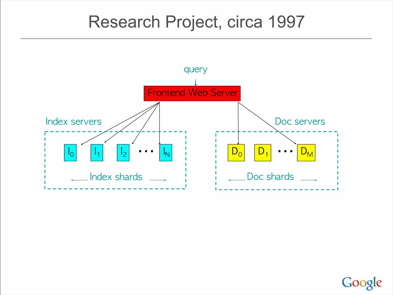
Research Project, circa 1997
Frontend Web Server
I0 I1 I2 IN
Index shards
D0 D1 DM
query
Index servers Doc servers
⋯ ⋯Doc shards
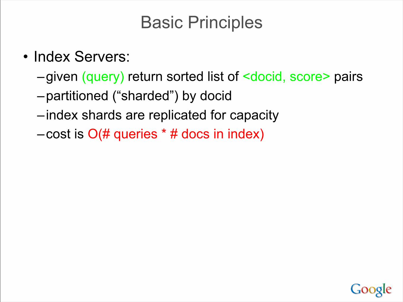
• Index Servers:–given (query) return sorted list of <docid, score> pairs–partitioned (“sharded”) by docid–index shards are replicated for capacity–cost is O(# queries * # docs in index)
Basic Principles
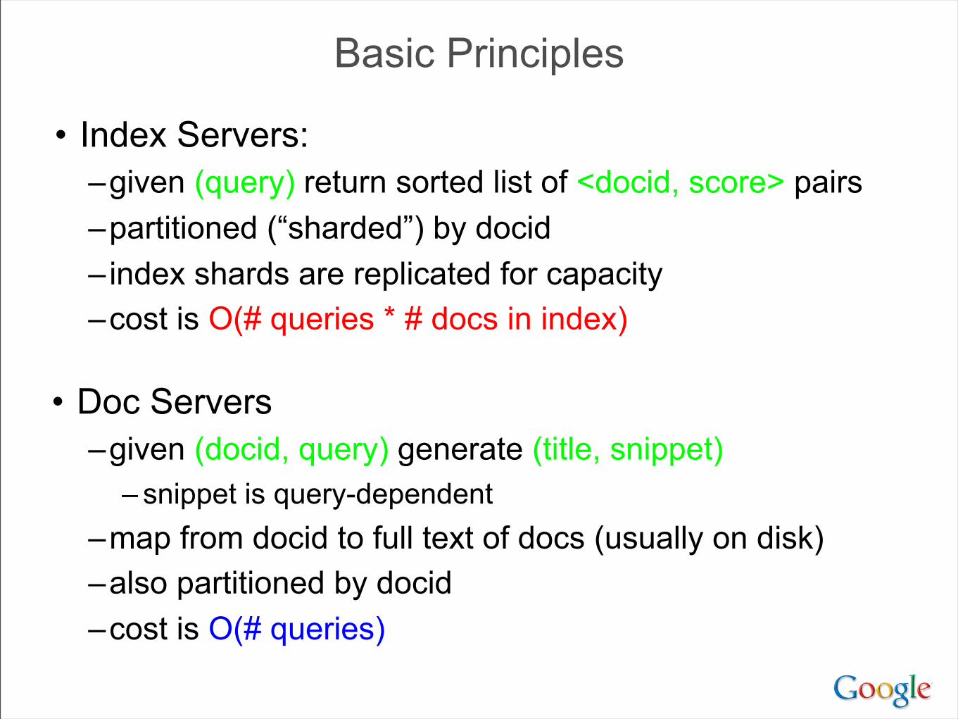
• Index Servers:–given (query) return sorted list of <docid, score> pairs–partitioned (“sharded”) by docid–index shards are replicated for capacity–cost is O(# queries * # docs in index)
Basic Principles
• Doc Servers–given (docid, query) generate (title, snippet)
– snippet is query-dependent–map from docid to full text of docs (usually on disk)–also partitioned by docid–cost is O(# queries)

“Corkboards” (1999)
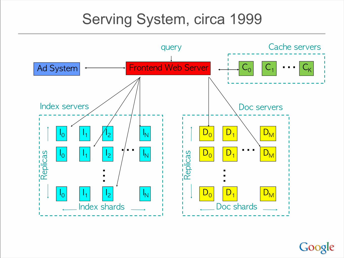
Serving System, circa 1999
Frontend Web Server
I0 I1 I2 IN
I0 I1 I2 IN
I0 I1 I2 IN
Replicas ⋯
⋯
Index shards
D0 D1 DM
D0 D1 DM
D0 D1 DMReplicas ⋯
⋯Doc shards
query
Index servers
Cache servers
C0 C1 CK⋯
Doc servers
Ad System
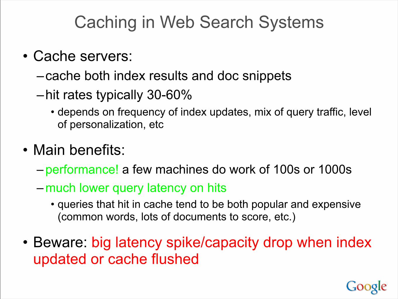
• Cache servers:–cache both index results and doc snippets–hit rates typically 30-60%
• depends on frequency of index updates, mix of query traffic, level of personalization, etc
• Main benefits:– performance! a few machines do work of 100s or 1000s– much lower query latency on hits
• queries that hit in cache tend to be both popular and expensive (common words, lots of documents to score, etc.)
• Beware: big latency spike/capacity drop when index updated or cache flushed
Caching in Web Search Systems

• Simple batch indexing system–No real checkpointing, so machine failures painful–No checksumming of raw data, so hardware bit errors
caused problems• Exacerbated by early machines having no ECC, no parity• Sort 1 TB of data without parity: ends up "mostly sorted"• Sort it again: "mostly sorted" another way
• “Programming with adversarial memory”–Developed file abstraction that stores checksums of
small records and can skip and resynchronize after corrupted records
Indexing (circa 1998-1999)
Google Data Center (2000)

Google Data Center (2000)
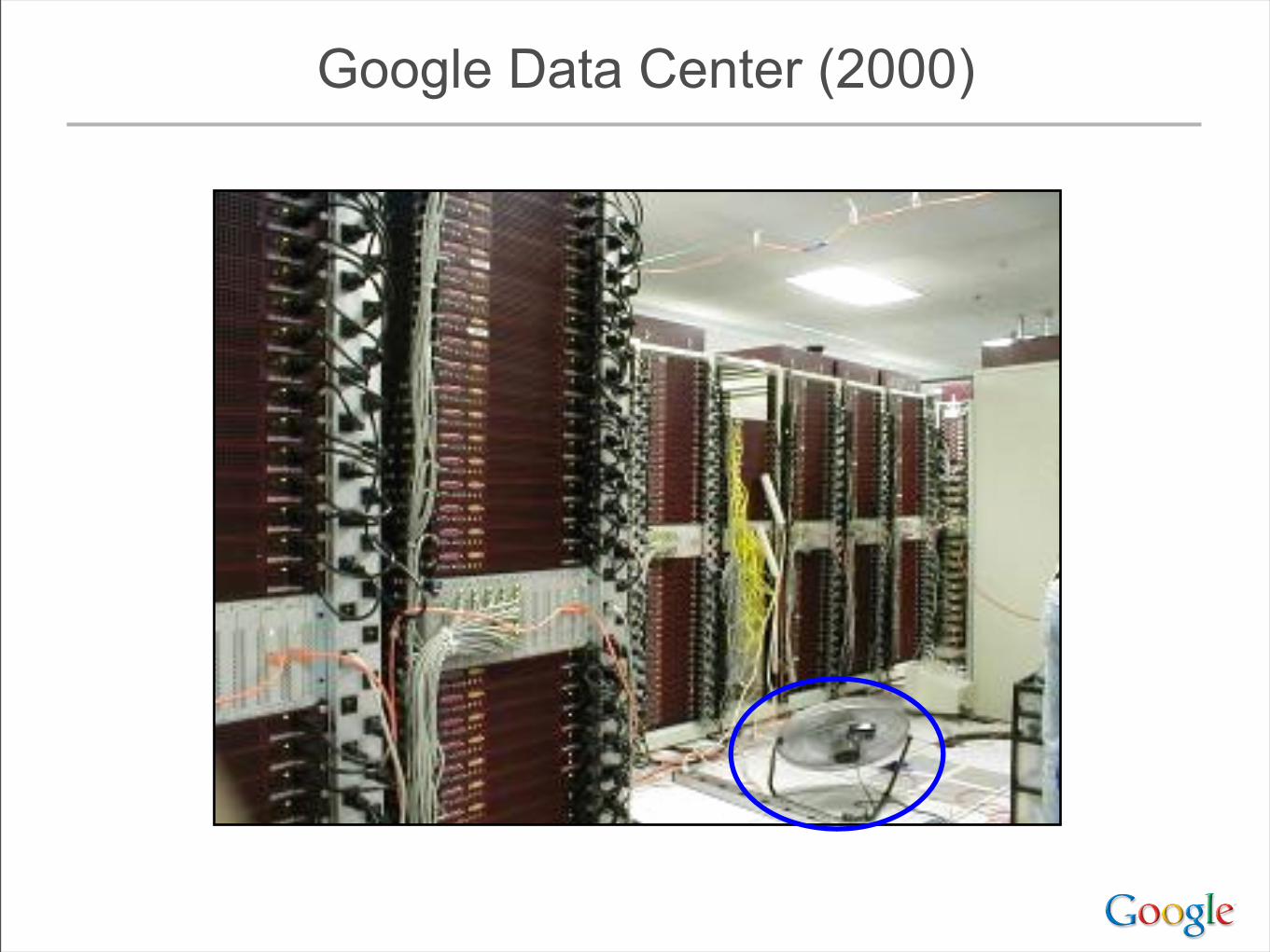
Google Data Center (2000)
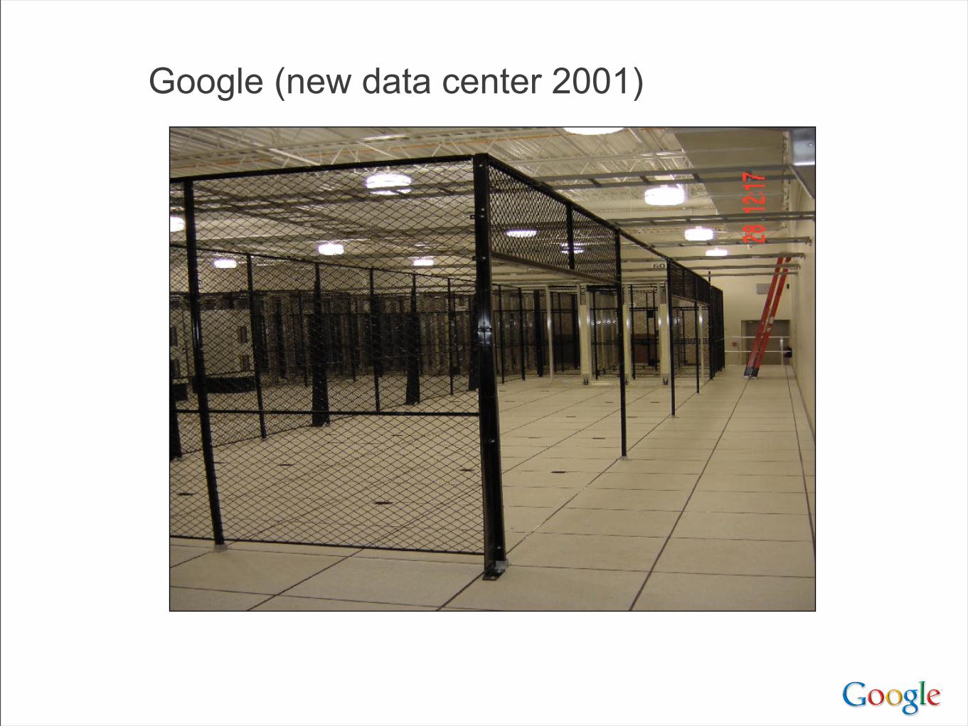
Google (new data center 2001)
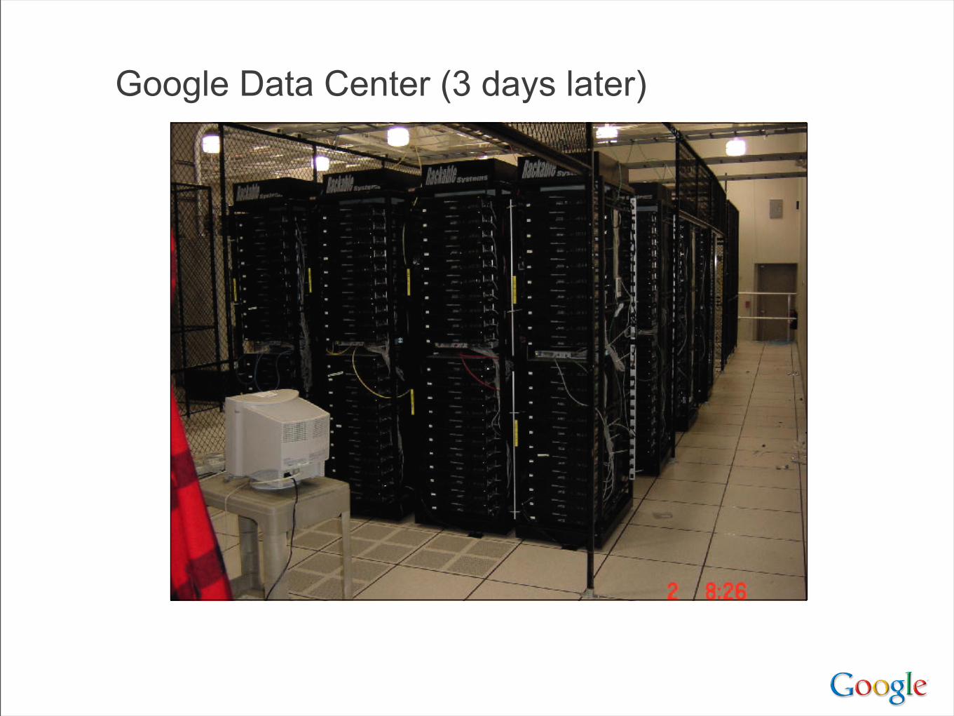
Google Data Center (3 days later)

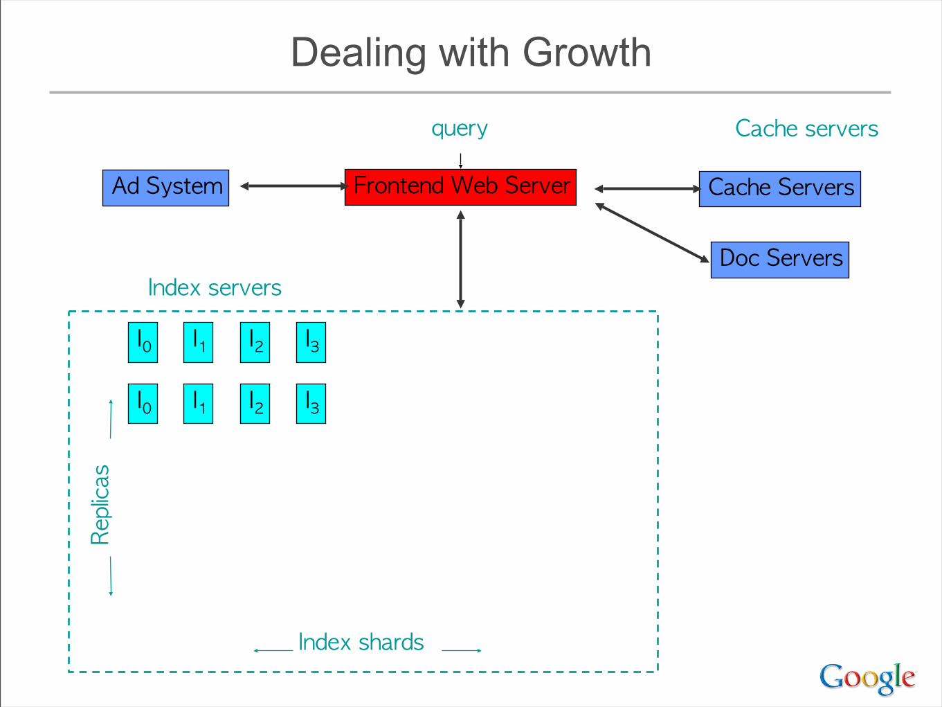
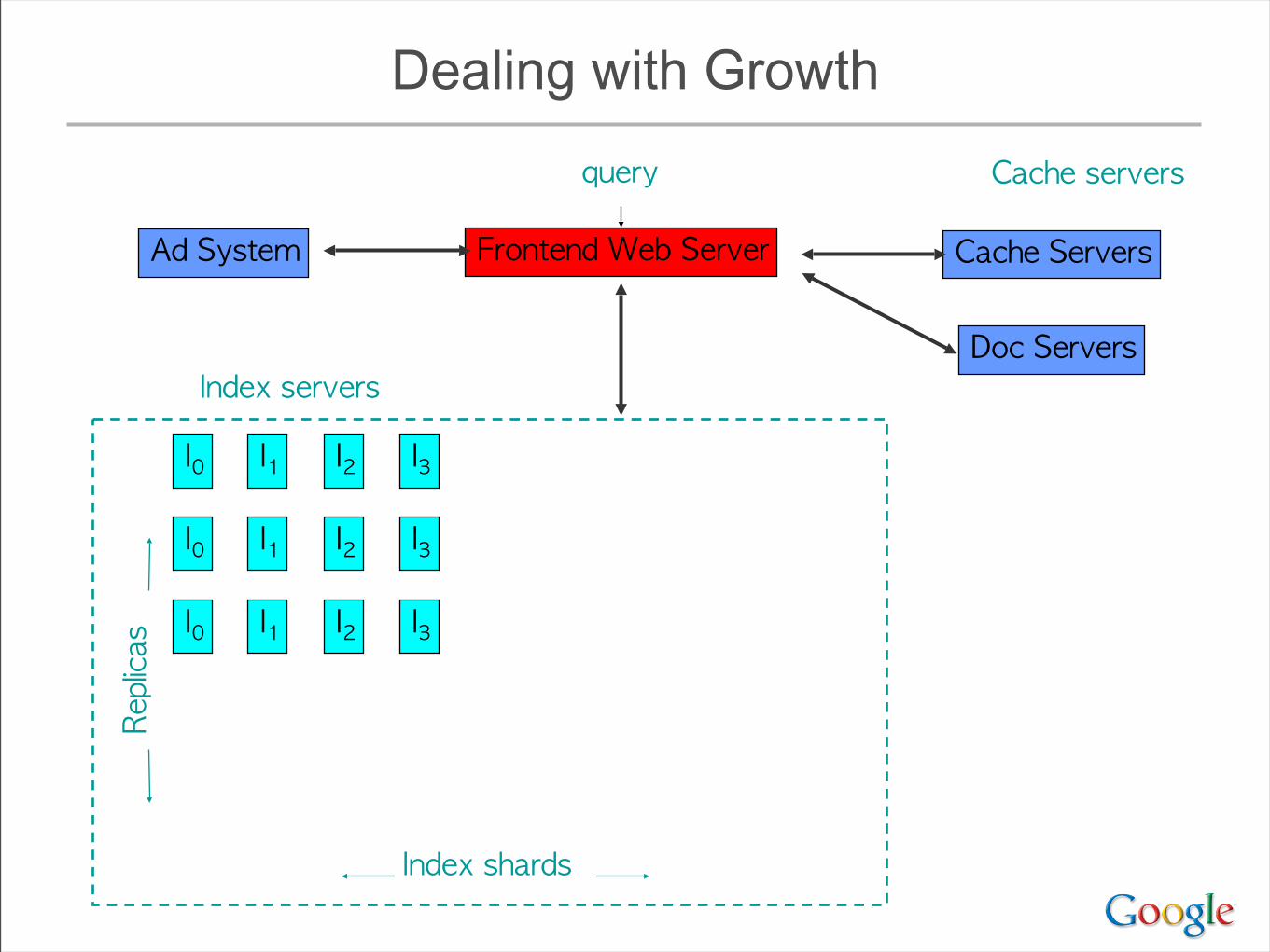
• Huge increases in index size in ’99, ’00, ’01, ...– From ~50M pages to more than 1000M pages
• At same time as huge traffic increases– ~20% growth per month in 1999, 2000, ...– ... plus major new partners (e.g. Yahoo in July 2000 doubled
traffic overnight)
• Performance of index servers was paramount– Deploying more machines continuously, but...– Needed ~10-30% software-based improvement every month
Increasing Index Size and Query Capacity

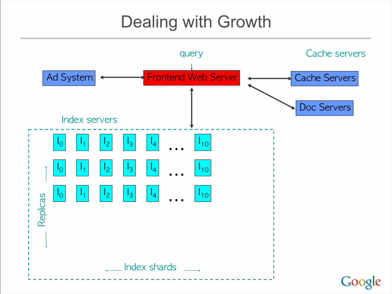
Dealing with Growth
Frontend Web Server
query
Index servers
Cache servers
Ad System
Doc Servers
Cache Servers
Replicas
Index shards
I0 I1 I2
I0 I1 I2
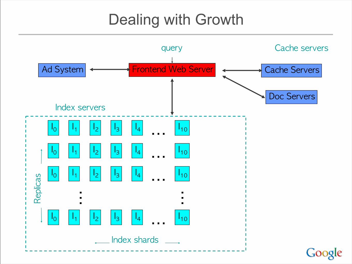
Dealing with Growth
Frontend Web Server
query
Index servers
Cache servers
Ad System
Doc Servers
Cache Servers
Replicas
Index shards
I0 I1 I2
I0 I1 I2
I3
I3
Dealing with Growth
Frontend Web Server
query
Index servers
Cache servers
Ad System
Doc Servers
Cache Servers
Replicas
Index shards
I0 I1 I2
I0 I1 I2
I3
I3
I0 I1 I2 I3

Dealing with Growth
Frontend Web Server
query
Index servers
Cache servers
Ad System
Doc Servers
Cache Servers
Replicas
Index shards
I0 I1 I2
I0 I1 I2
I3
I3
I0 I1 I2 I3
I4
I4
I4
Dealing with Growth
Frontend Web Server
query
Index servers
Cache servers
Ad System
Doc Servers
Cache Servers
Replicas
Index shards
I0 I1 I2
I0 I1 I2
I3
I3
I0 I1 I2 I3
I4
I4
I4
I10⋯I10⋯I10⋯
Dealing with Growth
Frontend Web Server
query
Index servers
Cache servers
Ad System
Doc Servers
Cache Servers
Replicas
Index shards
I0 I1 I2
I0 I1 I2
I3
I3
I0 I1 I2 I3
I4
I4
I4
I10⋯I10⋯I10⋯
I0 I1 I2 I3 I4 I10⋯
⋯ ⋯

Dealing with Growth
Frontend Web Server
query
Index servers
Cache servers
Ad System
Doc Servers
Cache Servers
Replicas
Index shards
I0 I1 I2
I0 I1 I2
I3
I3
I0 I1 I2 I3
I4
I4
I4
I10⋯I10⋯I10⋯
I0 I1 I2 I3 I4 I10⋯
⋯ ⋯
I60⋯I60⋯I60⋯I60⋯
⋯
# of disk seeks is O(#shards*#terms/query)
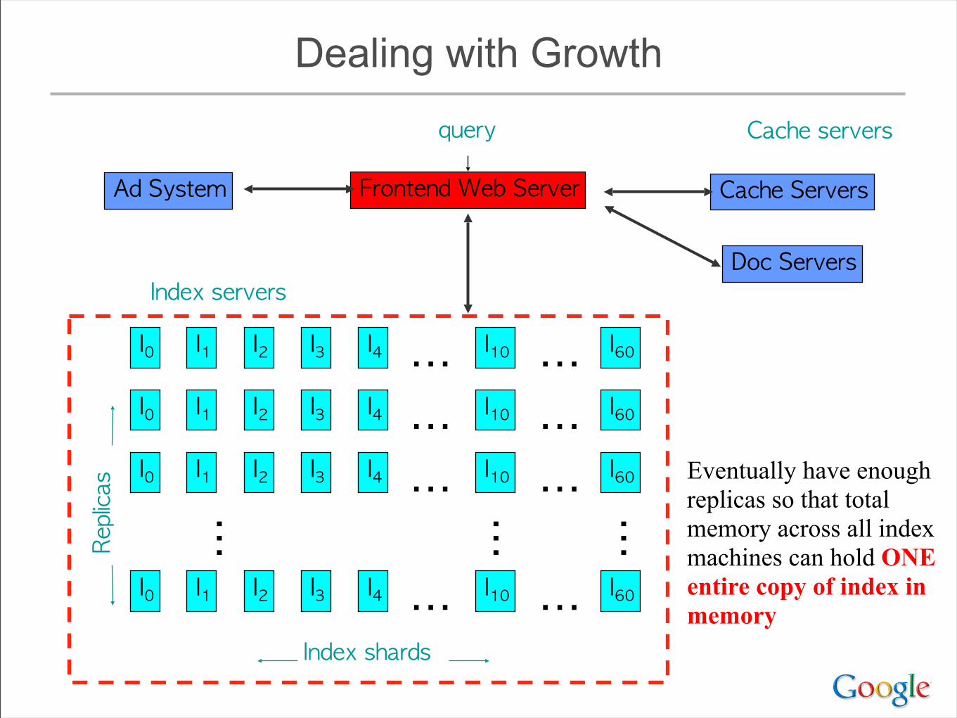
Dealing with Growth
Frontend Web Server
query
Index servers
Cache servers
Ad System
Doc Servers
Cache Servers
Replicas
Index shards
I0 I1 I2
I0 I1 I2
I3
I3
I0 I1 I2 I3
I4
I4
I4
I10⋯I10⋯I10⋯
I0 I1 I2 I3 I4 I10⋯
⋯ ⋯
I60⋯I60⋯I60⋯I60⋯
⋯
# of disk seeks is O(#shards*#terms/query)
Eventually have enough replicas so that total memory across all index machines can hold ONE entire copy of index in memory

Early 2001: In-Memory Index
Frontend Web Server
query
Index servers
Cache servers
Ad System
Doc Servers
Cache Servers
Index shards
Shard 0
I0 I1 I2
I14
I3
I12
bal
I4 I5
⋯I13
Shard 1
I0 I1 I2
I14
I3
I12
bal
I4 I5
⋯I13
Shard 2
I0 I1 I2
I14
I3
I12
bal
I4 I5
⋯I13
Shard N
I0 I1 I2
I14
I3
I12
bal
I4 I5
⋯I13
Balancers
⋯

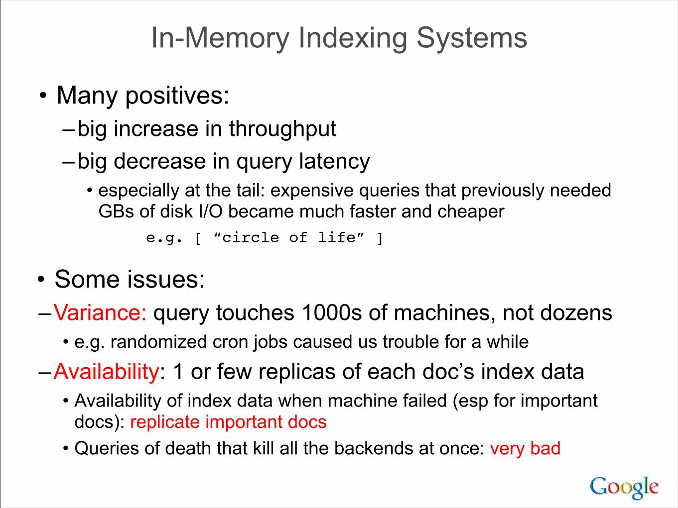
• Many positives:–big increase in throughput–big decrease in query latency
• especially at the tail: expensive queries that previously needed GBs of disk I/O became much faster and cheaper
e.g. [ “circle of life” ]
In-Memory Indexing Systems
• Many positives:–big increase in throughput–big decrease in query latency
• especially at the tail: expensive queries that previously needed GBs of disk I/O became much faster and cheaper
e.g. [ “circle of life” ]
In-Memory Indexing Systems
• Some issues:–Variance: query touches 1000s of machines, not dozens
• e.g. randomized cron jobs caused us trouble for a while
–Availability: 1 or few replicas of each doc’s index data• Availability of index data when machine failed (esp for important
docs): replicate important docs • Queries of death that kill all the backends at once: very bad
Canary Requests
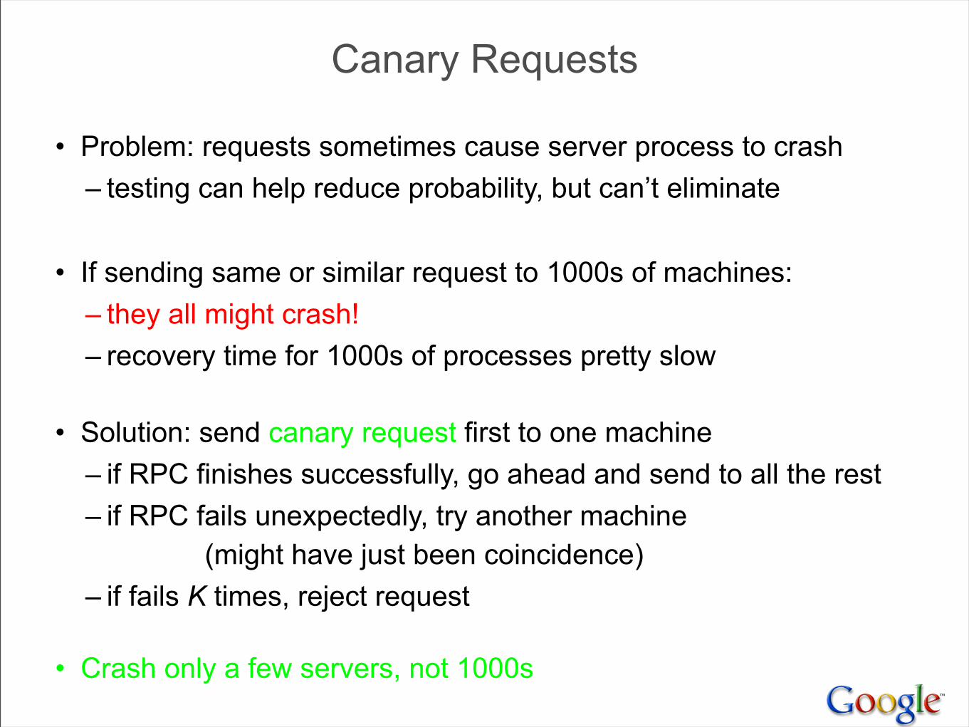
• Problem: requests sometimes cause server process to crash– testing can help reduce probability, but can’t eliminate
• If sending same or similar request to 1000s of machines:– they all might crash!– recovery time for 1000s of processes pretty slow
• Solution: send canary request first to one machine– if RPC finishes successfully, go ahead and send to all the rest– if RPC fails unexpectedly, try another machine
(might have just been coincidence)– if fails K times, reject request
• Crash only a few servers, not 1000s

Query Serving System, 2004 edition
Root
…
…
ParentServers
……
LeafServers
Repository Shards…
RepositoryManager
FileLoaders
Cache serversRequests
GFS

Query Serving System, 2004 edition
Root
…
…
ParentServers
……
LeafServers
Repository Shards…
RepositoryManager
FileLoaders
Cache serversRequests
GFS
Multi-level tree for query distribution

Query Serving System, 2004 edition
Root
…
…
ParentServers
……
LeafServers
Repository Shards…
RepositoryManager
FileLoaders
Cache serversRequests
GFS
Multi-level tree for query distribution
Leaf servers handle both index & doc requests from in-memory data structures

Query Serving System, 2004 edition
Root
…
…
ParentServers
……
LeafServers
Repository Shards…
RepositoryManager
FileLoaders
Cache serversRequests
GFS
Coordinates indexswitching as new shardsbecome available
Multi-level tree for query distribution
Leaf servers handle both index & doc requests from in-memory data structures

Features
• Clean abstractions:–Repository–Document–Attachments–Scoring functions
• Easy experimentation–Attach new doc and index data without full reindexing
• Higher performance: designed from ground up to assume data is in memory
New Index Format
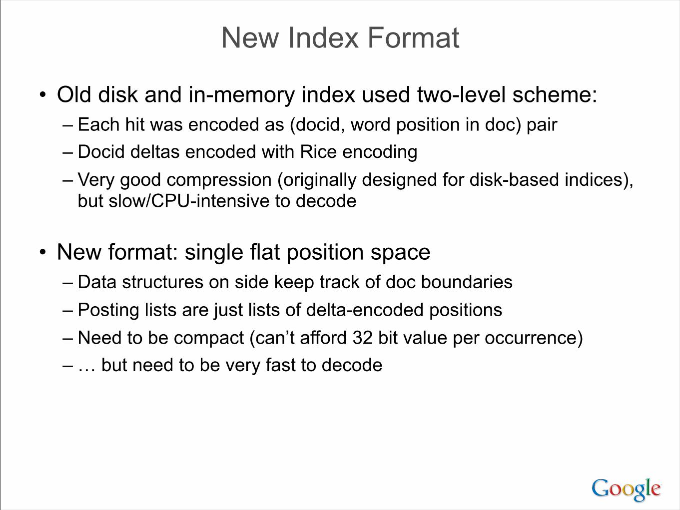
• Old disk and in-memory index used two-level scheme: – Each hit was encoded as (docid, word position in doc) pair– Docid deltas encoded with Rice encoding– Very good compression (originally designed for disk-based indices),
but slow/CPU-intensive to decode
• New format: single flat position space– Data structures on side keep track of doc boundaries– Posting lists are just lists of delta-encoded positions– Need to be compact (can’t afford 32 bit value per occurrence)– … but need to be very fast to decode
Byte-Aligned Variable-length Encodings
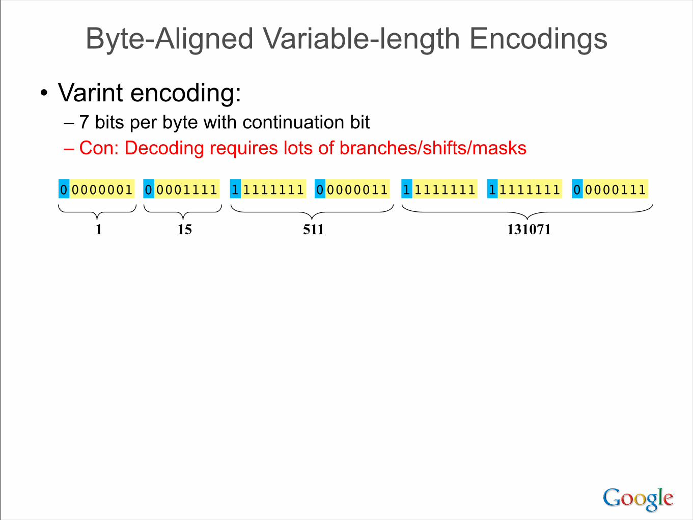
• Varint encoding:– 7 bits per byte with continuation bit– Con: Decoding requires lots of branches/shifts/masks
0000111100000001 0000001111111111 1111111111111111 00000111
1 15 511 131071
Byte-Aligned Variable-length Encodings
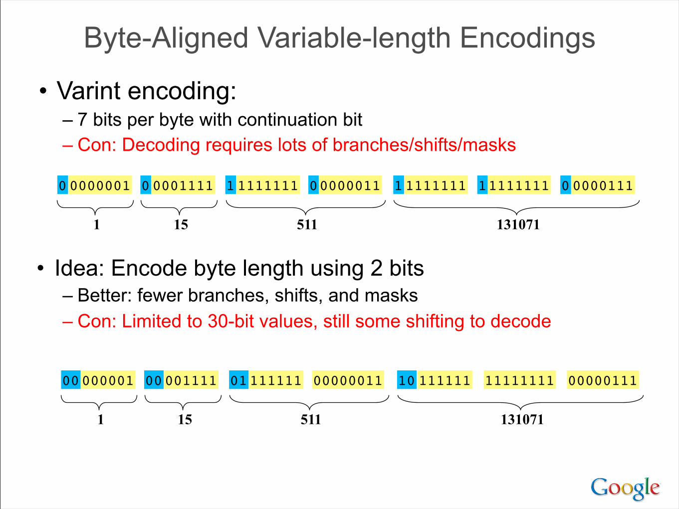
• Varint encoding:– 7 bits per byte with continuation bit– Con: Decoding requires lots of branches/shifts/masks
0000111100000001 0000001111111111 1111111111111111 00000111
1 15 511 131071
• Idea: Encode byte length using 2 bits– Better: fewer branches, shifts, and masks– Con: Limited to 30-bit values, still some shifting to decode
0000111100000001 0000001101111111 1111111110 111111 00000111
1 15 511 131071
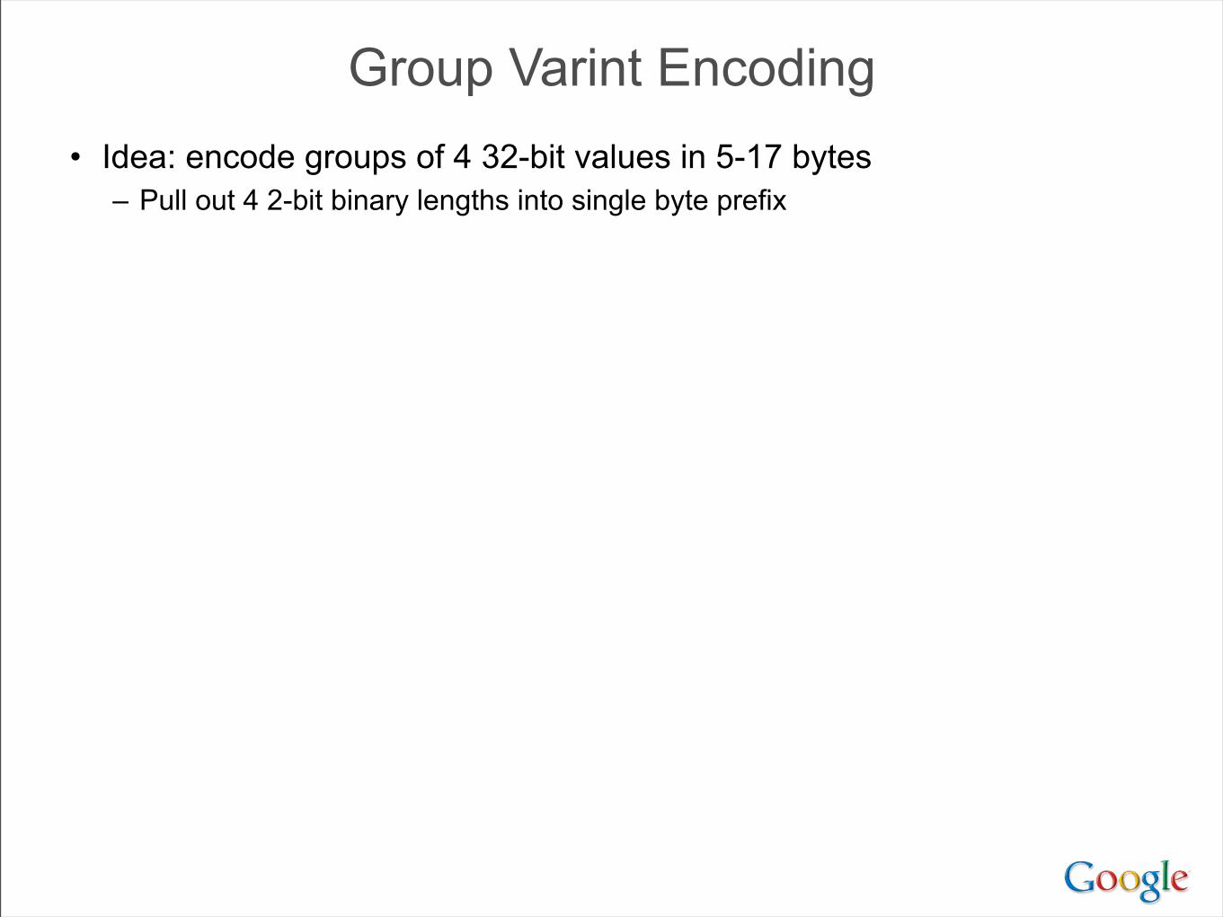
Group Varint Encoding• Idea: encode groups of 4 32-bit values in 5-17 bytes
– Pull out 4 2-bit binary lengths into single byte prefix

Group Varint Encoding• Idea: encode groups of 4 32-bit values in 5-17 bytes
– Pull out 4 2-bit binary lengths into single byte prefix
0000111100000001 0000011101111111 1111111110 111111 00000111

Group Varint Encoding• Idea: encode groups of 4 32-bit values in 5-17 bytes
– Pull out 4 2-bit binary lengths into single byte prefix
0000111100000001 0000011101111111 1111111110 111111 00000111
00000110
Tags
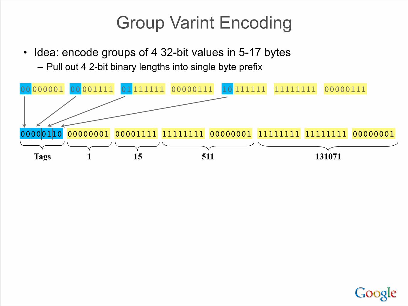
Group Varint Encoding• Idea: encode groups of 4 32-bit values in 5-17 bytes
– Pull out 4 2-bit binary lengths into single byte prefix
0000111100000001 0000011101111111 1111111110 111111 00000111
0000111100000001 11111111 11111111
1 15 511 131071
00000001 11111111 0000000100000110
Tags
Group Varint Encoding• Idea: encode groups of 4 32-bit values in 5-17 bytes
– Pull out 4 2-bit binary lengths into single byte prefix
0000111100000001 0000011101111111 1111111110 111111 00000111
0000111100000001 11111111 11111111
1 15 511 131071
00000001 11111111 0000000100000110
Tags
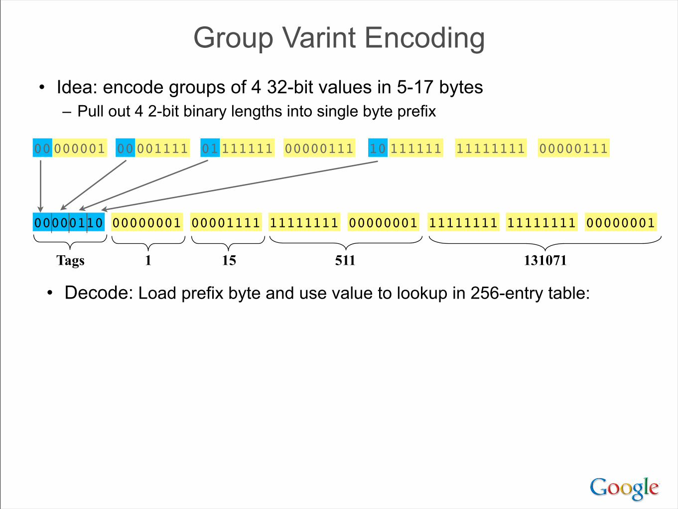
• Decode: Load prefix byte and use value to lookup in 256-entry table:

Group Varint Encoding• Idea: encode groups of 4 32-bit values in 5-17 bytes
– Pull out 4 2-bit binary lengths into single byte prefix
0000111100000001 0000011101111111 1111111110 111111 00000111
0000111100000001 11111111 11111111
1 15 511 131071
00000001 11111111 0000000100000110
Tags
• Decode: Load prefix byte and use value to lookup in 256-entry table:
00000110 Offsets: +1,+2,+3,+5; Masks: ff, ff, ffff, ffffff⋯⋯

Group Varint Encoding• Idea: encode groups of 4 32-bit values in 5-17 bytes
– Pull out 4 2-bit binary lengths into single byte prefix
0000111100000001 0000011101111111 1111111110 111111 00000111
0000111100000001 11111111 11111111
1 15 511 131071
00000001 11111111 0000000100000110
Tags
• Much faster than alternatives:– 7-bit-per-byte varint: decode ~180M numbers/second– 30-bit Varint w/ 2-bit length: decode ~240M numbers/second– Group varint: decode ~400M numbers/second
• Decode: Load prefix byte and use value to lookup in 256-entry table:
00000110 Offsets: +1,+2,+3,+5; Masks: ff, ff, ffff, ffffff⋯⋯

2007: Universal Search
Frontend Web Server
query
Cache servers
Ad System
News
Super root
Images
Web
BlogsVideo
Books
Local
Indexing Service
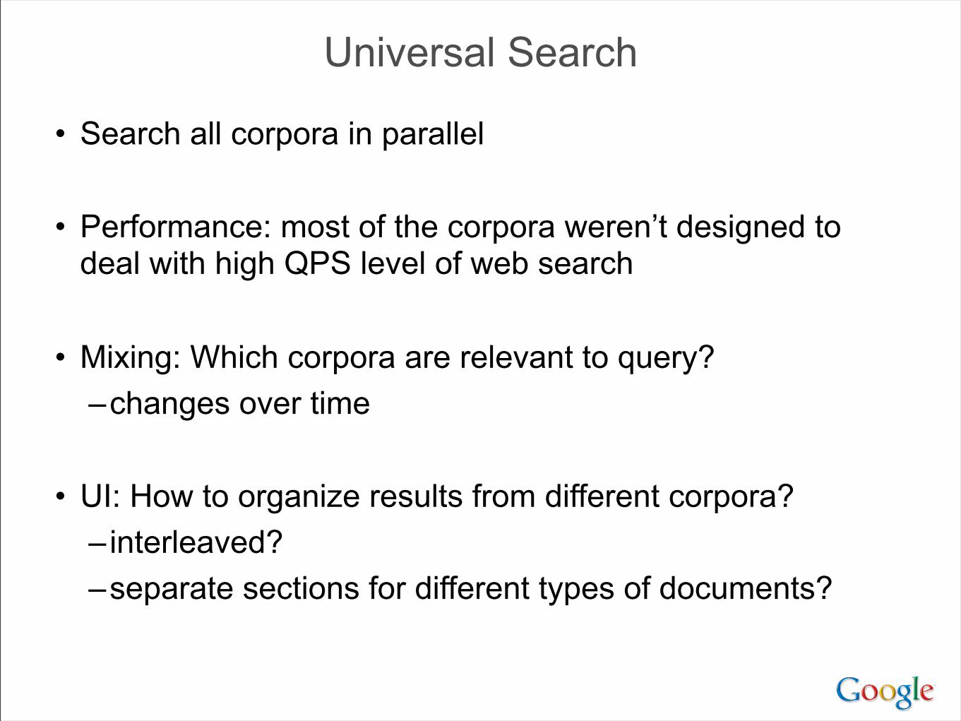
Universal Search
• Search all corpora in parallel
• Performance: most of the corpora weren’t designed to deal with high QPS level of web search
• Mixing: Which corpora are relevant to query?–changes over time
• UI: How to organize results from different corpora?–interleaved?–separate sections for different types of documents?

System Software Evolution

Machines + Racks
• In-house rack design• PC-class motherboards• Low-end storage & networking
hardware• Linux• + in-house software
Clusters
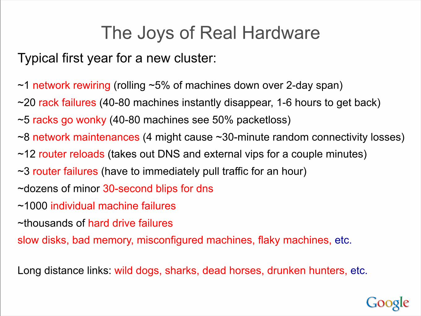
The Joys of Real HardwareTypical first year for a new cluster:
~1 network rewiring (rolling ~5% of machines down over 2-day span)~20 rack failures (40-80 machines instantly disappear, 1-6 hours to get back)~5 racks go wonky (40-80 machines see 50% packetloss)~8 network maintenances (4 might cause ~30-minute random connectivity losses)~12 router reloads (takes out DNS and external vips for a couple minutes)~3 router failures (have to immediately pull traffic for an hour)~dozens of minor 30-second blips for dns~1000 individual machine failures~thousands of hard drive failuresslow disks, bad memory, misconfigured machines, flaky machines, etc.
Long distance links: wild dogs, sharks, dead horses, drunken hunters, etc.
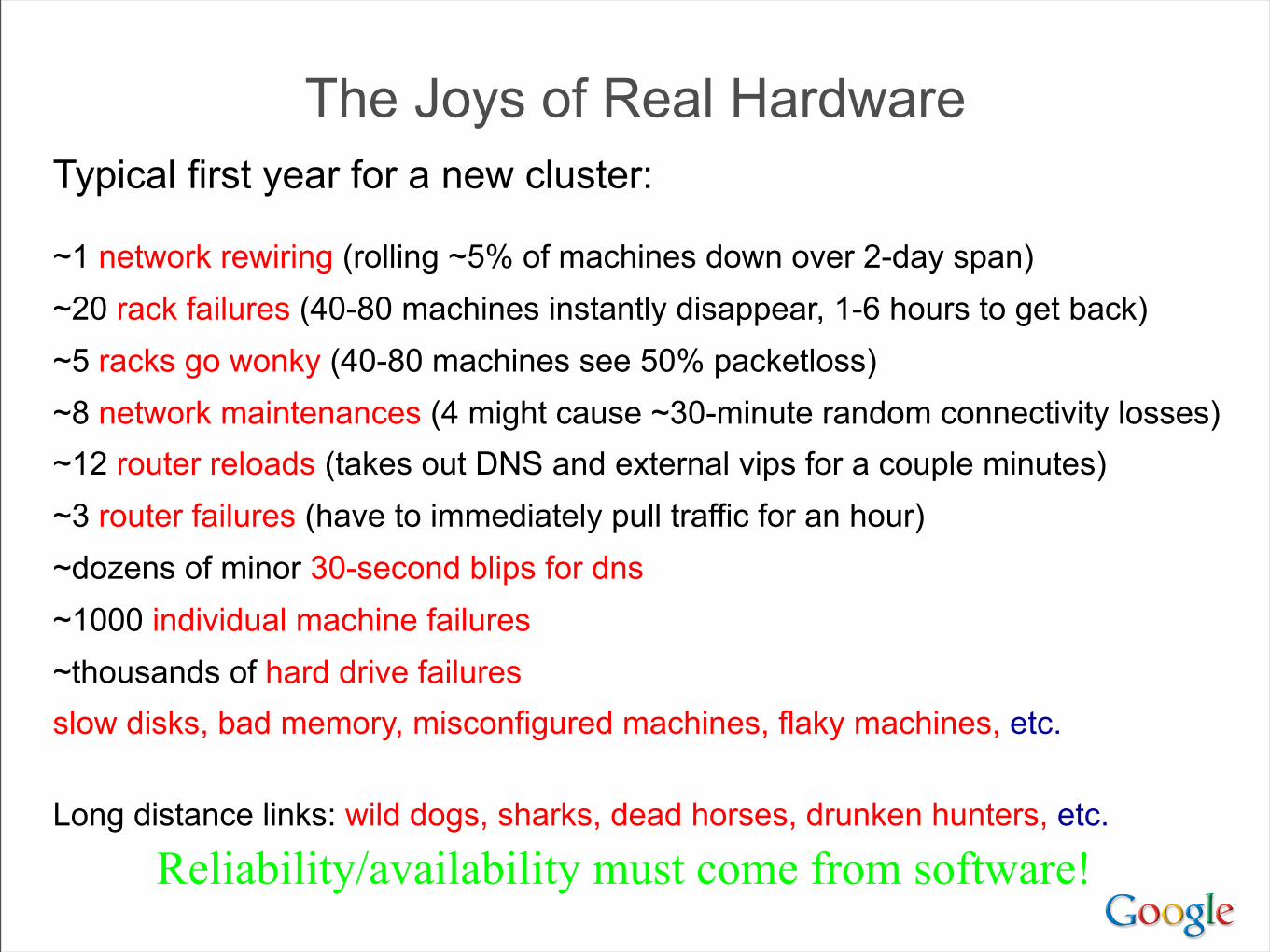
Reliability/availability must come from software!

Low-Level Systems Software Desires
• If you have lots of machines, you want to:
• Store data persistently–w/ high availability–high read and write bandwidth
• Run large-scale computations reliably–without having to deal with machine failures
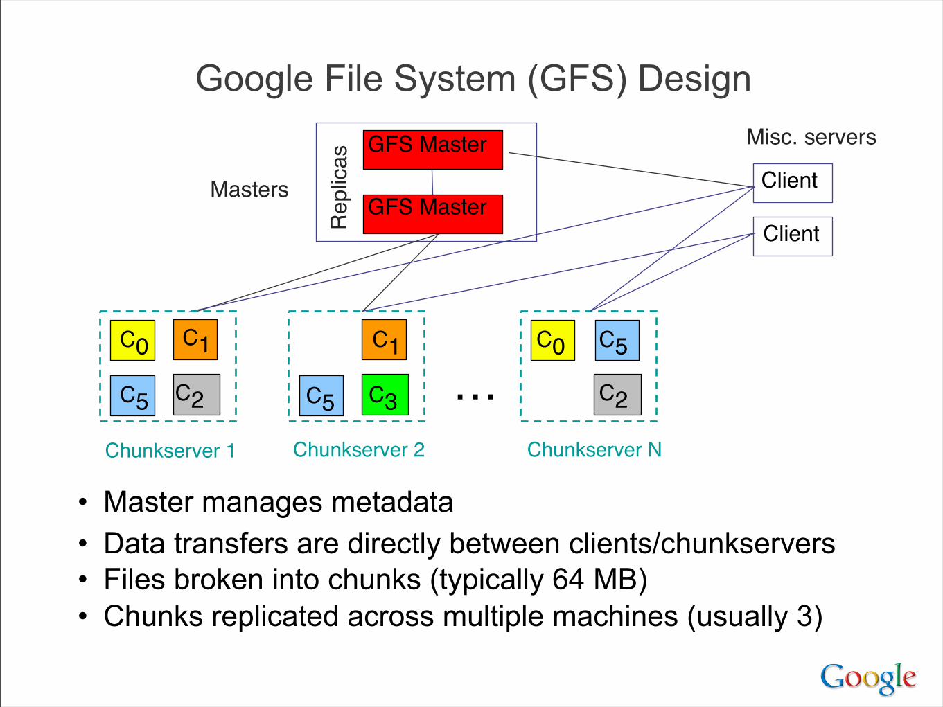
• Master manages metadata• Data transfers are directly between clients/chunkservers• Files broken into chunks (typically 64 MB)• Chunks replicated across multiple machines (usually 3)
Client
Client
Misc. servers
ClientRepl
icas
Masters
GFS Master
GFS Master
C0 C1
C2C5
Chunkserver 1
C0
C2
C5
Chunkserver N
C1
C3C5
Chunkserver 2
…
Google File System (GFS) Design

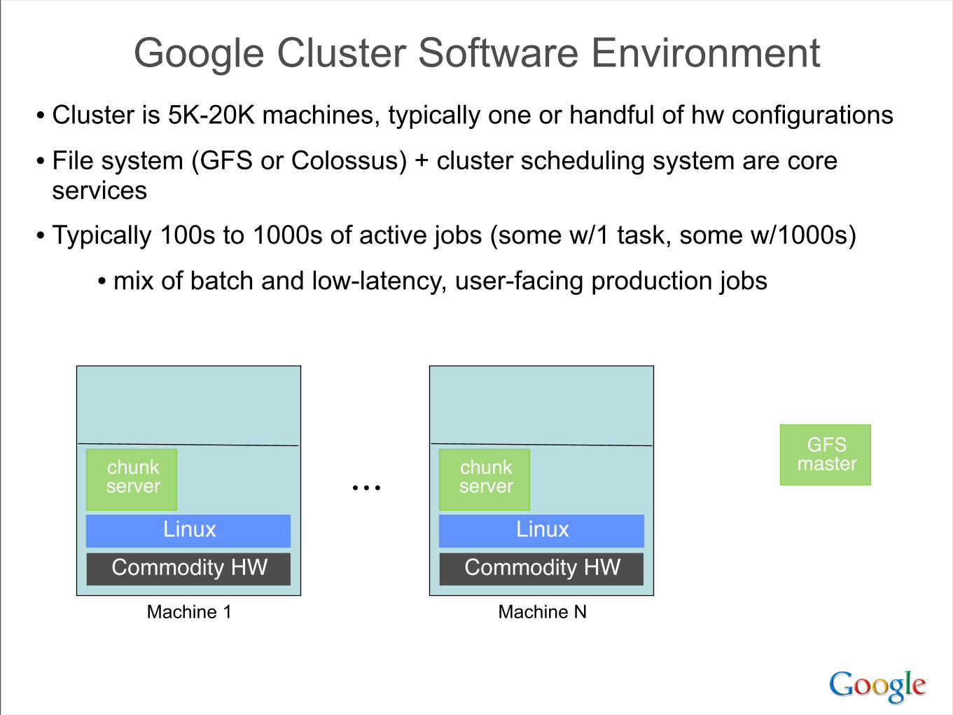
• Cluster is 5K-20K machines, typically one or handful of hw configurations
• File system (GFS or Colossus) + cluster scheduling system are core services
• Typically 100s to 1000s of active jobs (some w/1 task, some w/1000s)
• mix of batch and low-latency, user-facing production jobs
Google Cluster Software Environment
LinuxCommodity HW
LinuxCommodity HW
Machine 1
...
Machine N
chunkserver
chunkserver
GFSmaster

• Cluster is 5K-20K machines, typically one or handful of hw configurations
• File system (GFS or Colossus) + cluster scheduling system are core services
• Typically 100s to 1000s of active jobs (some w/1 task, some w/1000s)
• mix of batch and low-latency, user-facing production jobs
Google Cluster Software Environment
LinuxCommodity HW
LinuxCommodity HW
Machine 1
...
Machine N
schedulingdaemon
schedulingdaemon
schedulingmaster
chunkserver
chunkserver
GFSmaster
Chubbylock service

• Cluster is 5K-20K machines, typically one or handful of hw configurations
• File system (GFS or Colossus) + cluster scheduling system are core services
• Typically 100s to 1000s of active jobs (some w/1 task, some w/1000s)
• mix of batch and low-latency, user-facing production jobs
Google Cluster Software Environment
LinuxCommodity HW
LinuxCommodity HW
...job 1task
job 3task
job 12task
job 7task
job 3task
job 5task
Machine 1
...
Machine N
schedulingdaemon
schedulingdaemon
schedulingmaster
chunkserver
chunkserver
GFSmaster
Chubbylock service
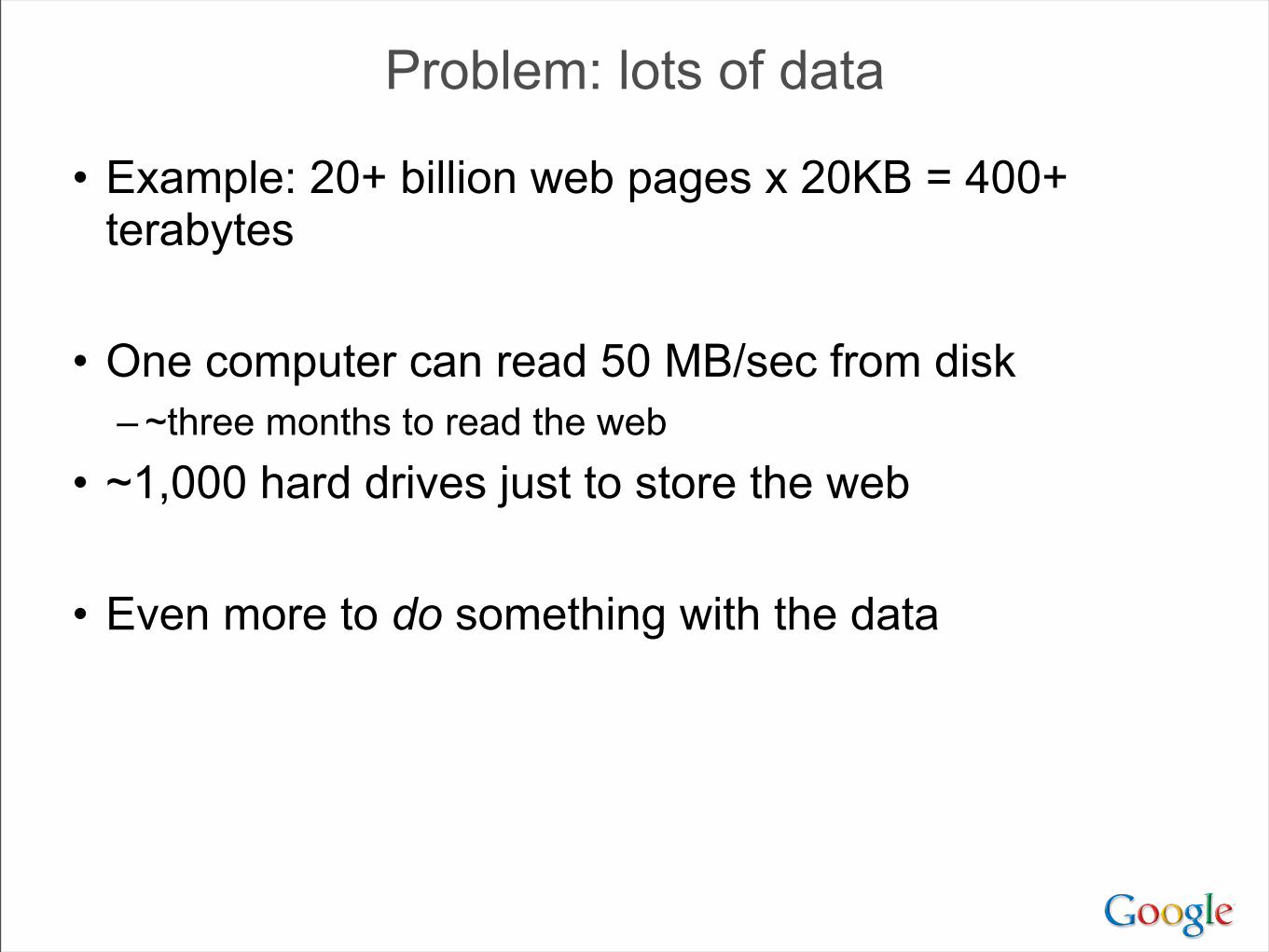
Problem: lots of data
• Example: 20+ billion web pages x 20KB = 400+ terabytes
• One computer can read 50 MB/sec from disk– ~three months to read the web
• ~1,000 hard drives just to store the web
• Even more to do something with the data

Solution: spread work over many machines
• Good news: same problem with 1000 machines, < 3 hours
• Bad news: programming work– communication and coordination– recovering from machine failure– status reporting– debugging– optimization– locality
• Bad news II: repeat for every problem you want to solve
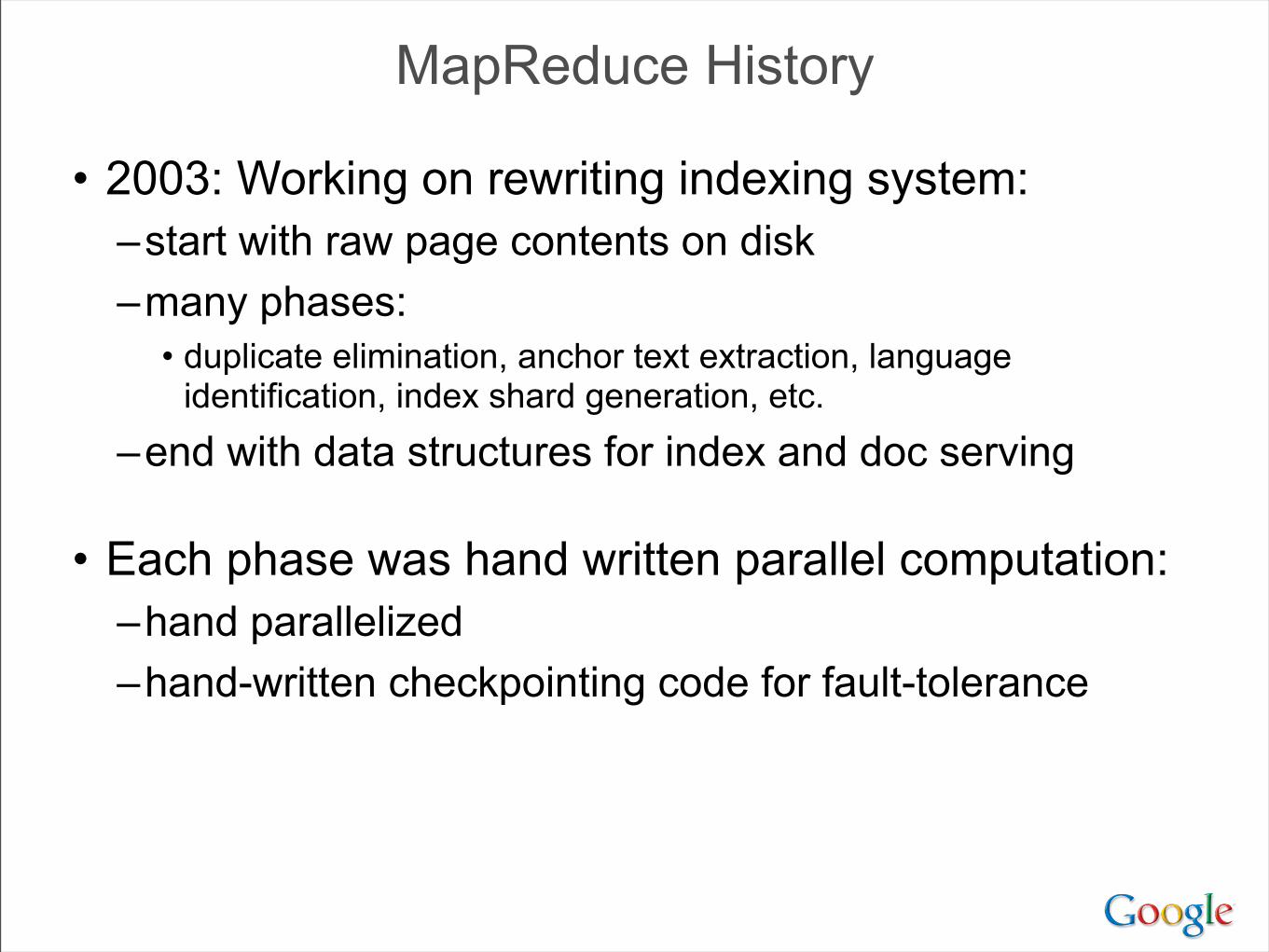
MapReduce History
• 2003: Working on rewriting indexing system:–start with raw page contents on disk–many phases:
• duplicate elimination, anchor text extraction, language identification, index shard generation, etc.
–end with data structures for index and doc serving
• Each phase was hand written parallel computation:–hand parallelized–hand-written checkpointing code for fault-tolerance
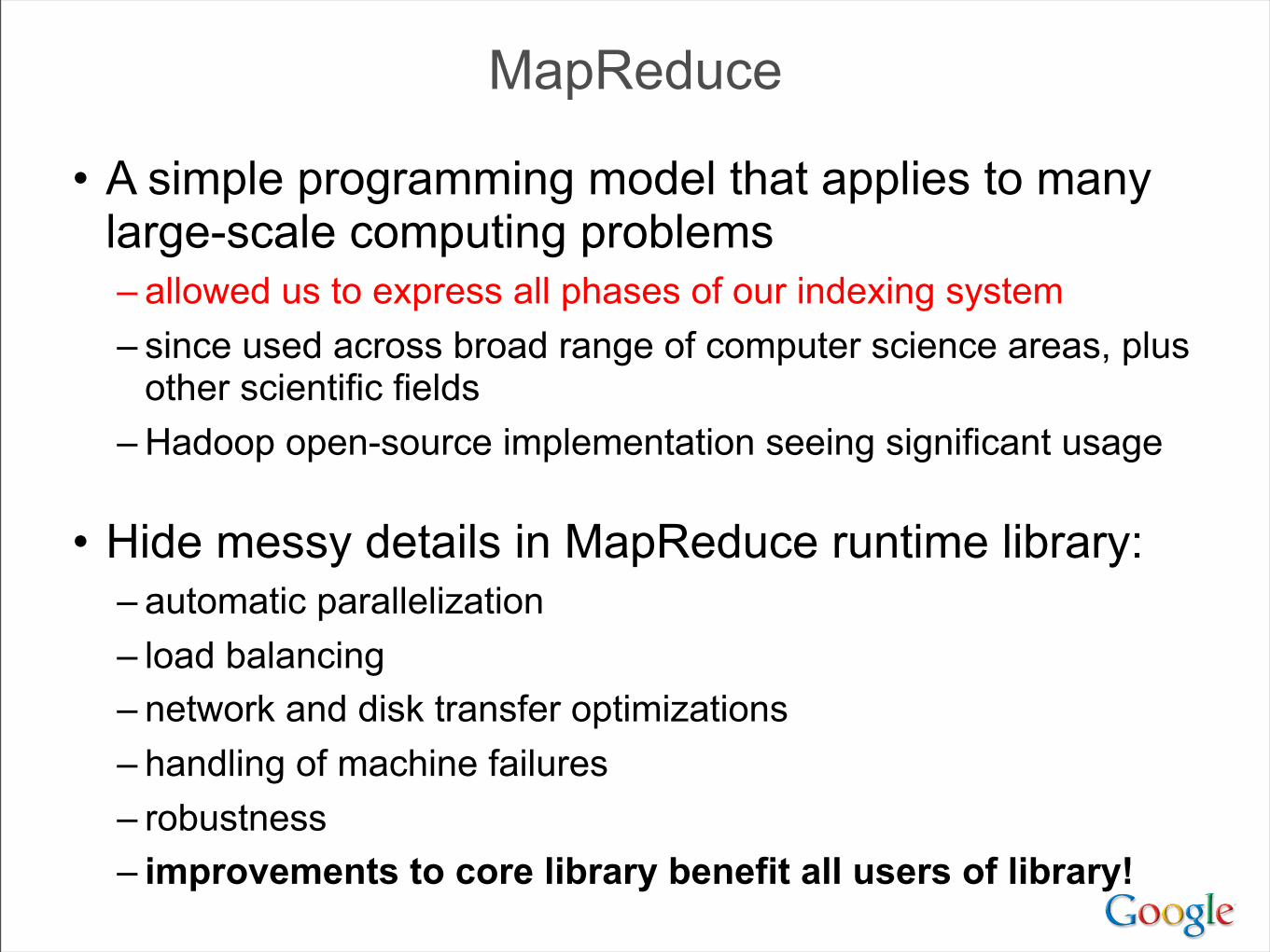
MapReduce
• A simple programming model that applies to many large-scale computing problems– allowed us to express all phases of our indexing system– since used across broad range of computer science areas, plus
other scientific fields– Hadoop open-source implementation seeing significant usage
• Hide messy details in MapReduce runtime library:– automatic parallelization– load balancing– network and disk transfer optimizations– handling of machine failures– robustness– improvements to core library benefit all users of library!
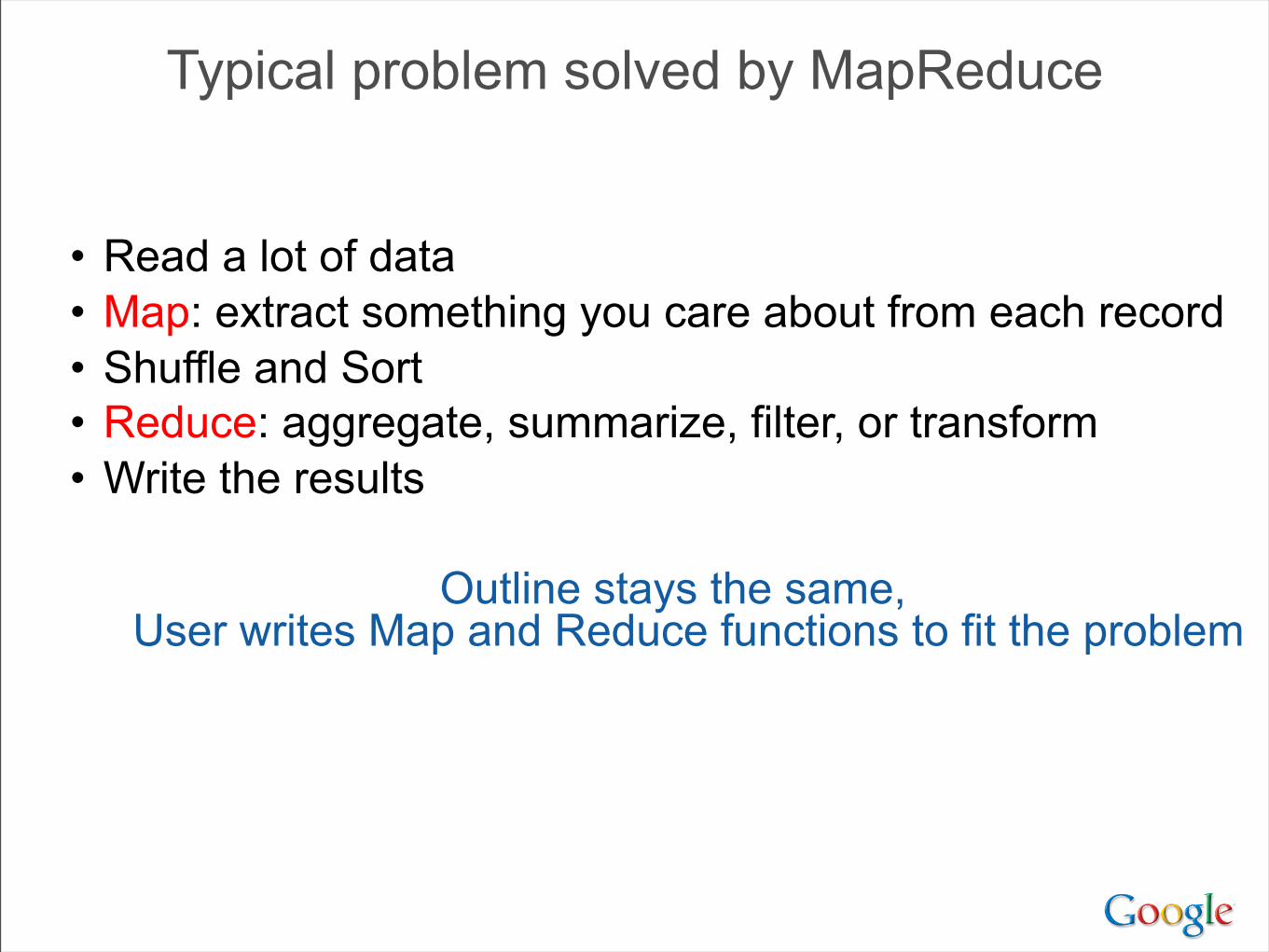
Typical problem solved by MapReduce
• Read a lot of data• Map: extract something you care about from each record• Shuffle and Sort• Reduce: aggregate, summarize, filter, or transform• Write the results
Outline stays the same,User writes Map and Reduce functions to fit the problem
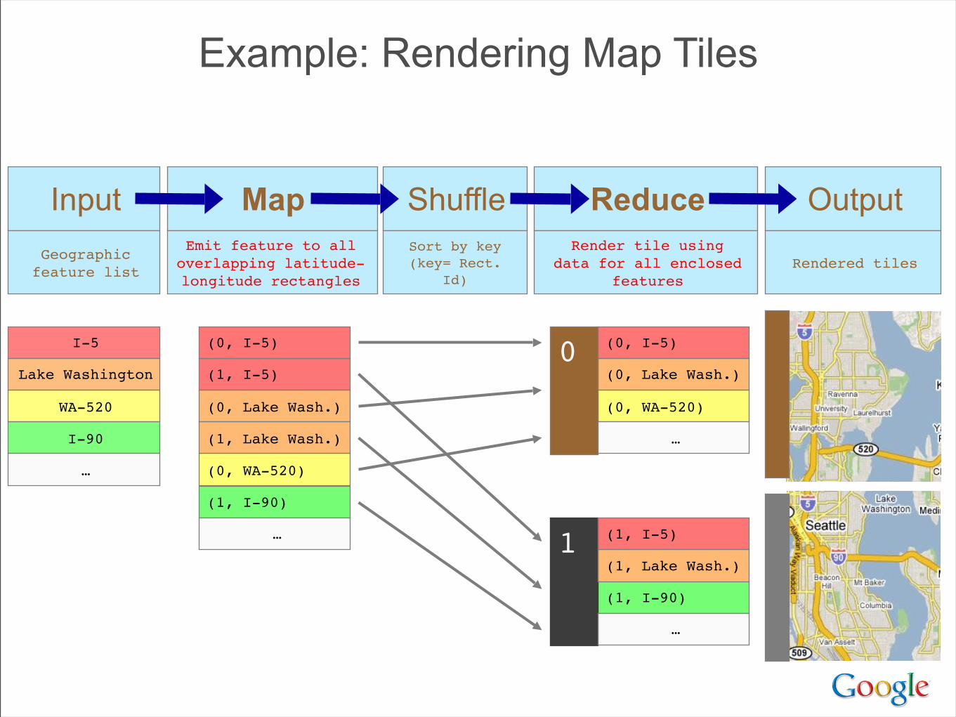
Example: Rendering Map Tiles
Input Map Shuffle Reduce OutputEmit feature to all
overlapping latitude-longitude rectangles
Sort by key(key= Rect.
Id)
Render tile usingdata for all enclosed
featuresRendered tiles
Geographicfeature list
I-5
Lake Washington
WA-520
I-90
(0, I-5)
(0, Lake Wash.)
(0, WA-520)
(1, I-90)
(1, I-5)
(1, Lake Wash.)
(0, I-5)
(0, Lake Wash.)
(0, WA-520)
(1, I-90)
0
1 (1, I-5)
(1, Lake Wash.)
…
…
…
…

MapReduce: Scheduling
• One master, many workers – Input data split into M map tasks (typically 64 MB in size)– Reduce phase partitioned into R reduce tasks– Tasks are assigned to workers dynamically– Often: M=200,000; R=4,000; workers=2,000
• Master assigns each map task to a free worker – Considers locality of data to worker when assigning task– Worker reads task input (often from local disk!)– Worker produces R local files containing intermediate k/v pairs
• Master assigns each reduce task to a free worker – Worker reads intermediate k/v pairs from map workers– Worker sorts & applies user’s Reduce op to produce the output

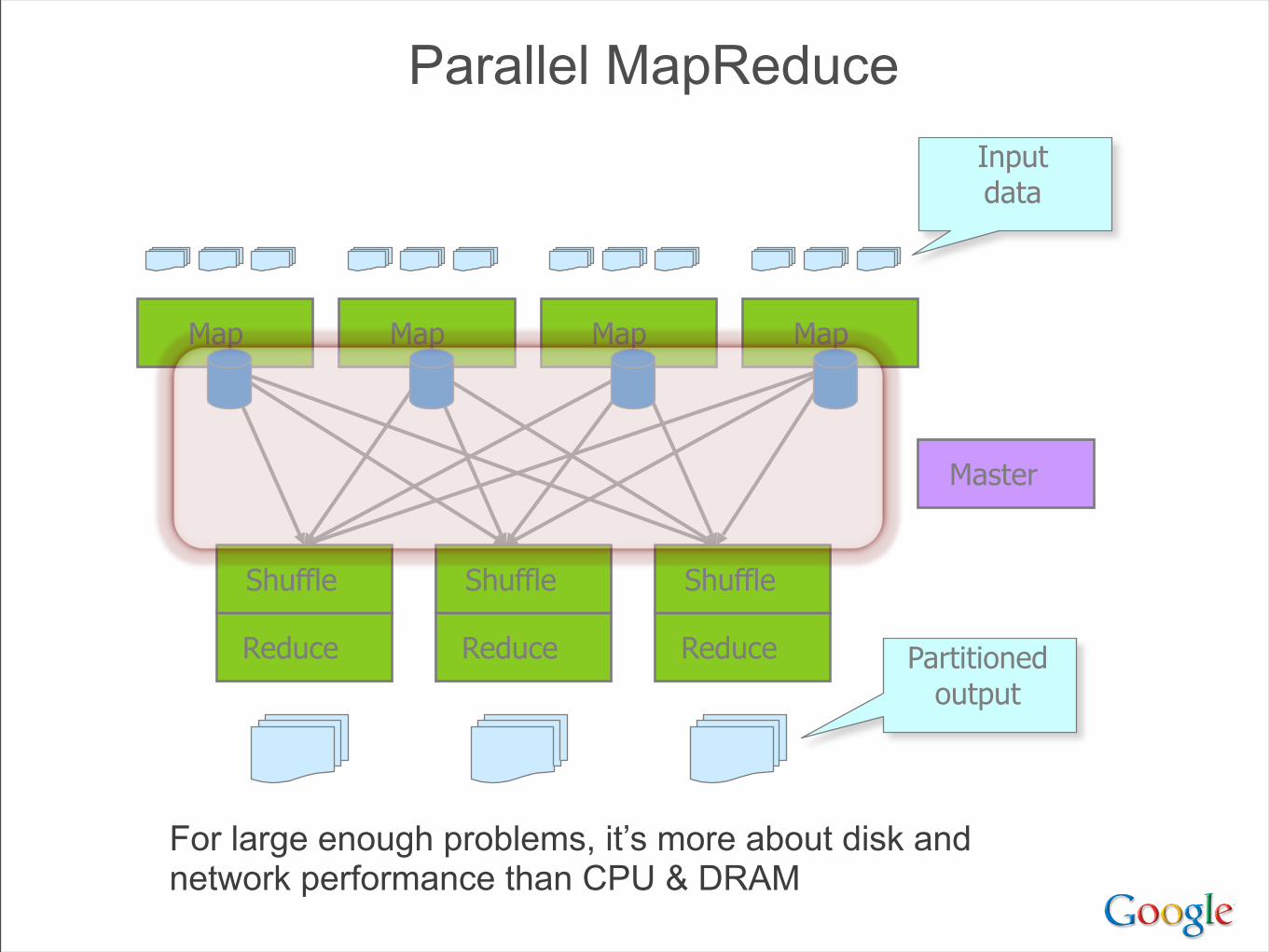
Parallel MapReduce
Map Map Map Map
Inputdata
Reduce
Shuffle
Reduce
Shuffle
Reduce
Shuffle
Partitioned output
Master
Parallel MapReduce
Map Map Map Map
Inputdata
Reduce
Shuffle
Reduce
Shuffle
Reduce
Shuffle
Partitioned output
Master
For large enough problems, it’s more about disk and network performance than CPU & DRAM
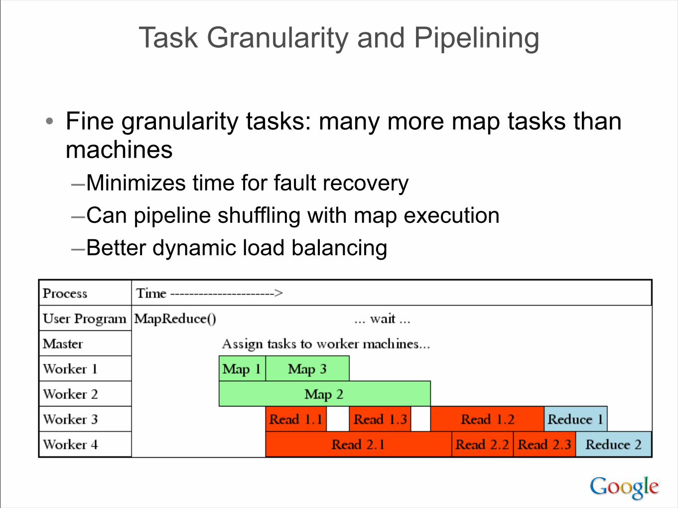
Task Granularity and Pipelining
• Fine granularity tasks: many more map tasks than machines–Minimizes time for fault recovery–Can pipeline shuffling with map execution–Better dynamic load balancing
• Often use 200,000 map/5000 reduce tasks w/ 2000 machines
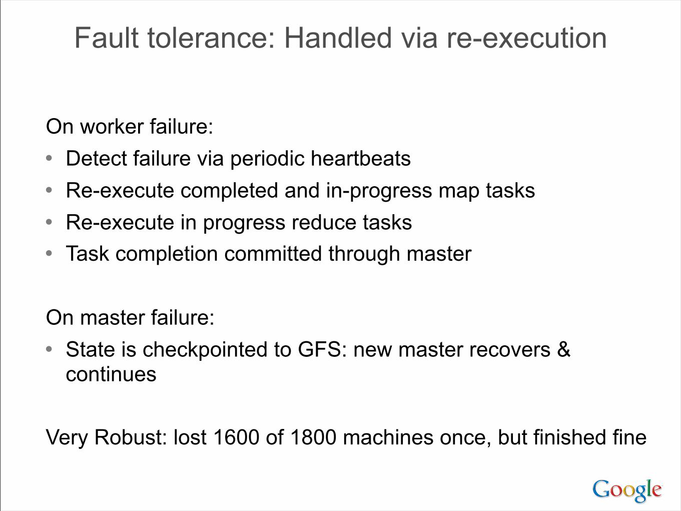
Fault tolerance: Handled via re-execution
On worker failure:• Detect failure via periodic heartbeats • Re-execute completed and in-progress map tasks• Re-execute in progress reduce tasks• Task completion committed through master
On master failure:• State is checkpointed to GFS: new master recovers &
continues
Very Robust: lost 1600 of 1800 machines once, but finished fine

Refinement: Backup Tasks
• Slow workers significantly lengthen completion time–Other jobs consuming resources on machine–Bad disks with soft errors transfer data very slowly–Weird things: processor caches disabled (!!)
• Solution: Near end of phase, spawn backup copies of tasks–Whichever one finishes first "wins"
• Effect: Dramatically shortens job completion time

Refinement: Locality Optimization
Master scheduling policy:• Asks GFS for locations of replicas of input file blocks• Map tasks typically split into 64MB (== GFS block size)• Map tasks scheduled so GFS input block replica are on
same machine or same rack
Effect: Thousands of machines read input at local disk speed
• Without this, rack switches limit read rate

MapReduce Usage Statistics Over Time
Number of jobsAug, ‘04
29KMar, ‘06
171KSep, '072,217K
May, ’104,474K
Average completion time (secs) 634 874 395 748
Machine years used 217 2,002 11,081 39,121
Input data read (TB) 3,288 52,254 403,152 946,460
Intermediate data (TB) 758 6,743 34,774 132,960
Output data written (TB) 193 2,970 14,018 45,720
Average worker machines 157 268 394 368

Current Work: Spanner
• Storage & computation system that runs across many datacenters– single global namespace
• names are independent of location(s) of data• fine-grained replication configurations
– support mix of strong and weak consistency across datacenters• Strong consistency implemented with Paxos across tablet replicas• Full support for distributed transactions across directories/machines
– much more automated operation• automatically changes replication based on constraints and usage patterns• automated allocation of resources across entire fleet of machines
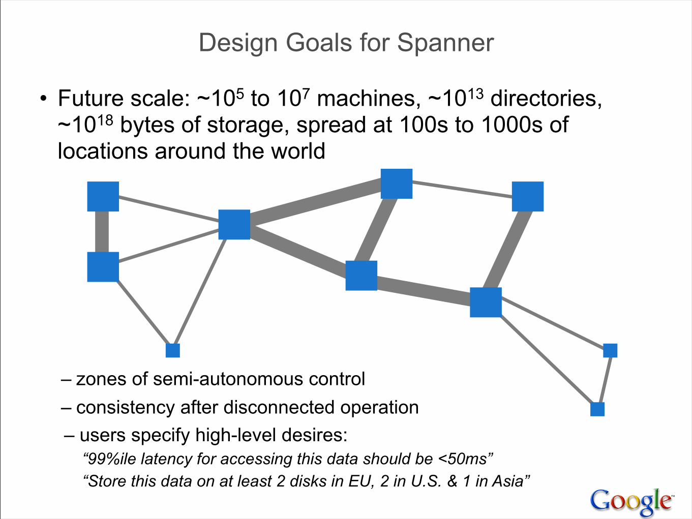
• Future scale: ~105 to 107 machines, ~1013 directories, ~1018 bytes of storage, spread at 100s to 1000s of locations around the world
– zones of semi-autonomous control– consistency after disconnected operation– users specify high-level desires:
“99%ile latency for accessing this data should be <50ms” “Store this data on at least 2 disks in EU, 2 in U.S. & 1 in Asia”
Design Goals for Spanner

System Building Experiences and Patterns
• Experiences from building a variety of systems–A collection of patterns that have emerged–Not all encompassing, obviously, but good rules of
thumb

Many Internal Services
• Break large complex systems down into many services!
• Simpler from a software engineering standpoint– few dependencies, clearly specified– easy to test and deploy new versions of individual services– ability to run lots of experiments– easy to reimplement service without affecting clients
• Development cycles largely decoupled– lots of benefits: small teams can work independently– easier to have many engineering offices around the world
• e.g. google.com search touches 200+ services–ads, web search, books, news, spelling correction, ...

Designing Efficient Systems
Given a basic problem definition, how do you choose "best" solution?
• Best might be simplest, highest performance, easiest to extend, etc.
Important skill: ability to estimate performance of a system design– without actually having to build it!

Numbers Everyone Should Know
L1 cache reference 0.5 ns
Branch mispredict 5 ns
L2 cache reference 7 ns
Mutex lock/unlock 25 ns
Main memory reference 100 ns
Compress 1K w/cheap compression algorithm 3,000 ns
Send 2K bytes over 1 Gbps network 20,000 ns
Read 1 MB sequentially from memory 250,000 ns
Round trip within same datacenter 500,000 ns
Disk seek 10,000,000 ns
Read 1 MB sequentially from disk 20,000,000 ns
Send packet CA->Netherlands->CA 150,000,000 ns

Back of the Envelope Calculations
How long to generate image results page (30 thumbnails)?
Design 1: Read serially, thumbnail 256K images on the fly30 seeks * 10 ms/seek + 30 * 256K / 30 MB/s = 560 ms

Back of the Envelope Calculations
How long to generate image results page (30 thumbnails)?
Design 1: Read serially, thumbnail 256K images on the fly30 seeks * 10 ms/seek + 30 * 256K / 30 MB/s = 560 ms
Design 2: Issue reads in parallel:10 ms/seek + 256K read / 30 MB/s = 18 ms
(Ignores variance, so really more like 30-60 ms, probably)
Lots of variations:– caching (single images? whole sets of thumbnails?)– pre-computing thumbnails– …
Back of the envelope helps identify most promising…

Know Your Basic Building Blocks
Core language libraries, basic data structures, protocol buffers, GFS, BigTable, indexing systems, MapReduce, …
Not just their interfaces, but understand their implementations (at least at a high level)
If you don’t know what’s going on, you can’t do decent back-of-the-envelope calculations!
Designing & Building InfrastructureIdentify common problems, and build software systems to
address them in a general way
• Important to not try to be all things to all people– Clients might be demanding 8 different things– Doing 6 of them is easy– …handling 7 of them requires real thought– …dealing with all 8 usually results in a worse system
• more complex, compromises other clients in trying to satisfy everyone

Designing & Building Infrastructure (cont)Don't build infrastructure just for its own sake:• Identify common needs and address them• Don't imagine unlikely potential needs that aren't really there
Best approach: use your own infrastructure (especially at first!)• (much more rapid feedback about what works, what doesn't)
Design for Growth
Try to anticipate how requirements will evolvekeep likely features in mind as you design base system
Don’t design to scale infinitely:~5X - 50X growth good to consider>100X probably requires rethink and rewrite

Pattern: Single Master, 1000s of Workers• Master orchestrates global operation of system
– load balancing, assignment of work, reassignment when machines fail, etc.
– ... but client interaction with master is fairly minimal
• Examples:– GFS, BigTable, MapReduce, file transfer service, cluster
scheduling system, ...
Client
Misc. serversRe
plica
sMasters
Master
MasterClient
Worker 1 Worker 2 Worker N
Client

Pattern: Single Master, 1000s of Workers (cont)
• Often: hot standby of master waiting to take over• Always: bulk of data transfer directly between clients and workers
• Pro:– simpler to reason about state of system with centralized master
• Caveats:– careful design required to keep master out of common case ops– scales to 1000s of workers, but not 100,000s of workers

• Problem: Single machine sending 1000s of RPCs overloads NIC on machine when handling replies– wide fan in causes TCP drops/retransmits, significant latency– CPU becomes bottleneck on single machine
Pattern: Tree Distribution of Requests
Root
Leaf 1 Leaf 2 Leaf 3 Leaf 4 Leaf 5 Leaf 6

• Solution: Use tree distribution of requests/responses– fan in at root is smaller– cost of processing leaf responses spread across many parents
• Most effective when parent processing can trim/combine leaf data– can also co-locate parents on same rack as leaves
Pattern: Tree Distribution of Requests
Root
Leaf 1 Leaf 2 Leaf 3 Leaf 4 Leaf 5 Leaf 6
Parent Parent
Pattern: Backup Requests to Minimize Latency
• Problem: variance high when requests go to 1000s of machines– last few machines to respond stretch out latency tail substantially
• Often, multiple replicas can handle same kind of request• When few tasks remaining, send backup requests to other replicas• Whichever duplicate request finishes first wins
– useful when variance is unrelated to specifics of request– increases overall load by a tiny percentage– decreases latency tail significantly
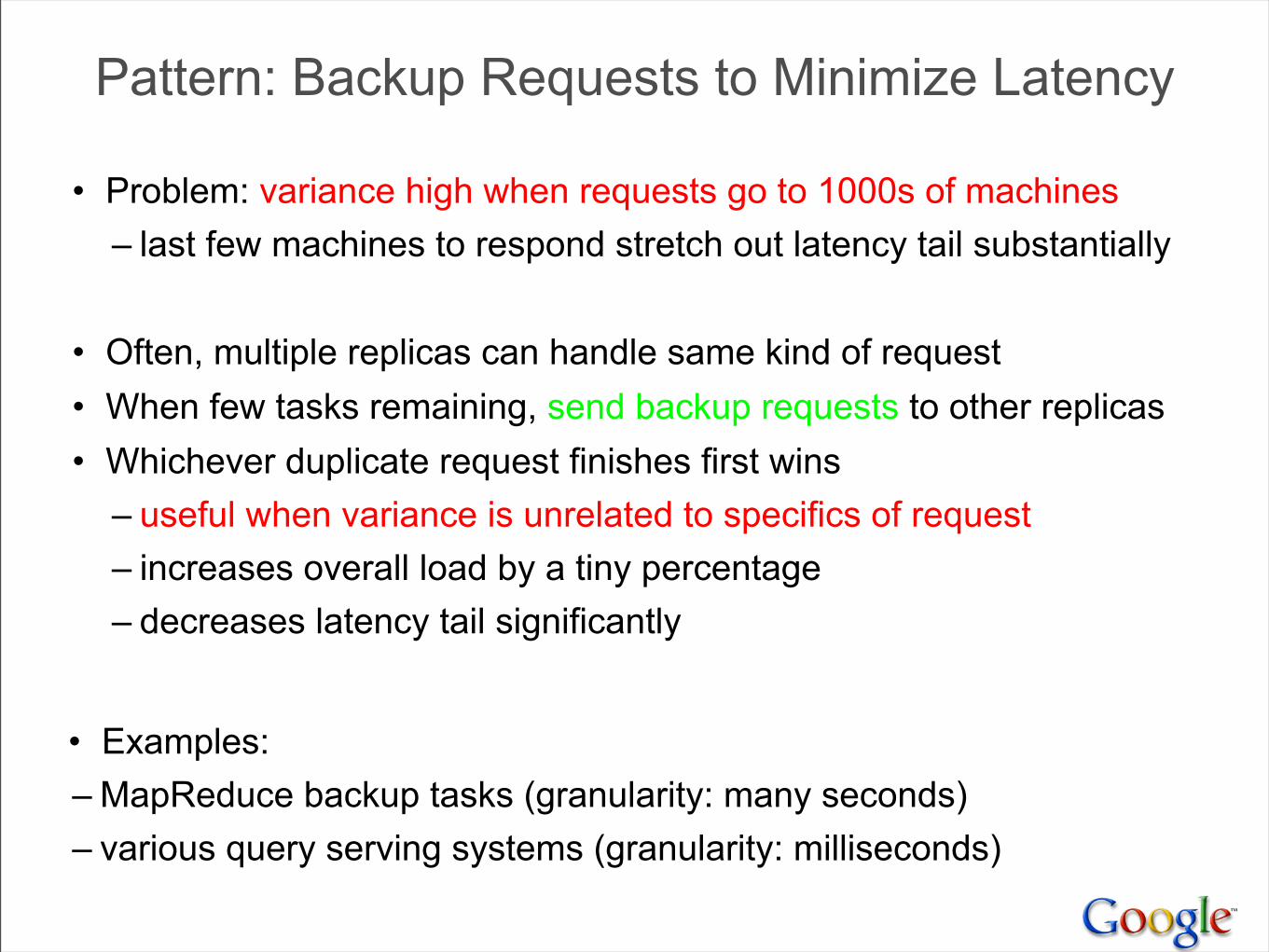
• Examples:– MapReduce backup tasks (granularity: many seconds)– various query serving systems (granularity: milliseconds)
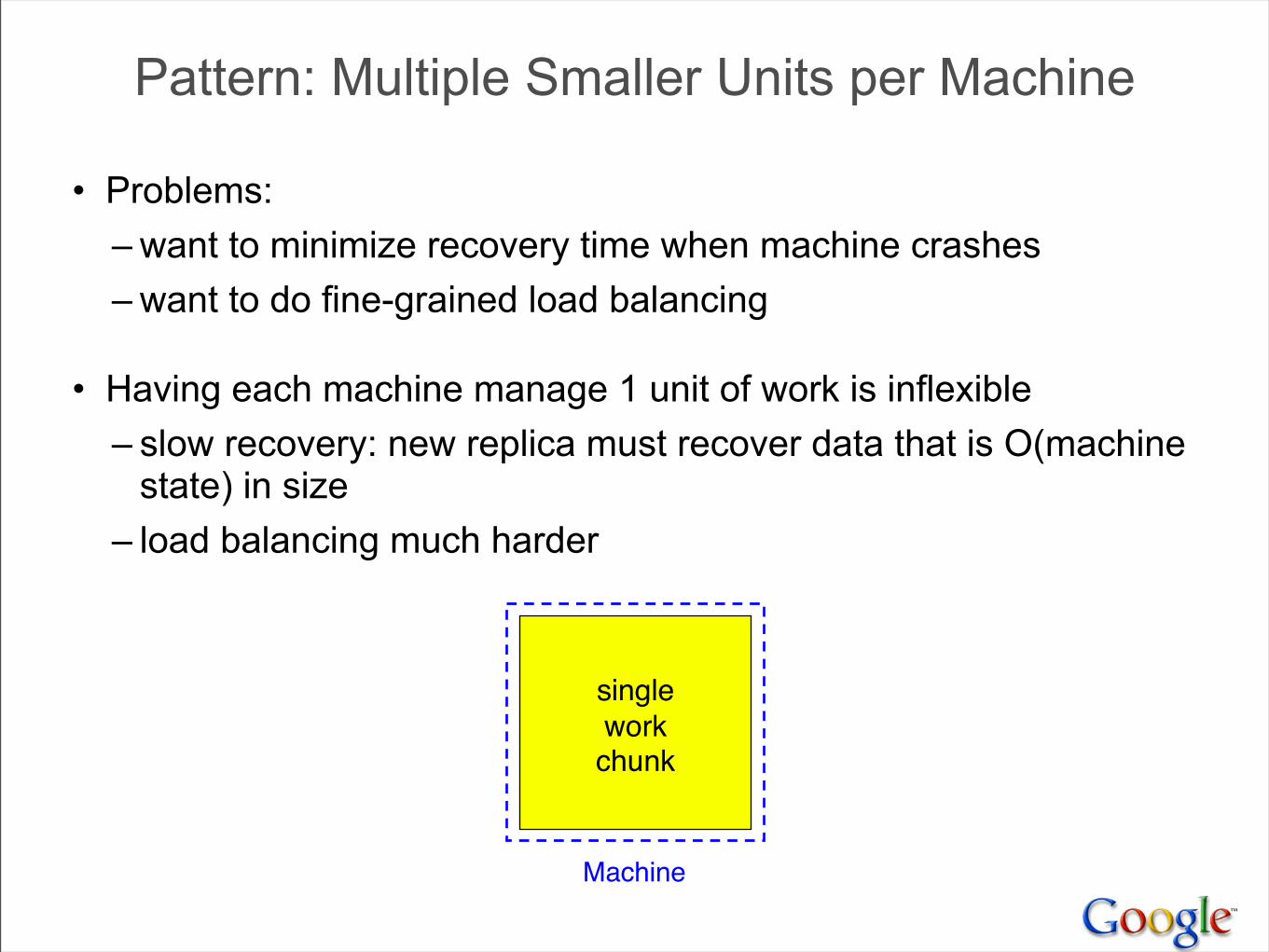
Pattern: Multiple Smaller Units per Machine
• Problems: – want to minimize recovery time when machine crashes– want to do fine-grained load balancing
• Having each machine manage 1 unit of work is inflexible– slow recovery: new replica must recover data that is O(machine
state) in size– load balancing much harder
singlework
chunk
Machine

Pattern: Multiple Smaller Units per Machine
• Have each machine manage many smaller units of work/data – typical: ~10-100 units/machine– allows fine grained load balancing (shed or add one unit)– fast recovery from failure (N machines each pick up 1 unit)
• Examples:– map and reduce tasks, GFS chunks, Bigtable tablets, query
serving system index shards
C0 C1
C2C5Machine
C9
C8
C17C6C11

Pattern: Elastic Systems
• Problem: Planning for exact peak load is hard– overcapacity: wasted resources– undercapacity: meltdown
• Design system to adapt:– automatically shrink capacity during idle period– automatically grow capacity as load grows
• Make system resilient to overload:– do something reasonable even up to 2X planned capacity
• e.g. shrink size of index searched, back off to less CPU intensive algorithms, drop spelling correction tips, etc.
– more aggressive load balancing when imbalance more severe

Pattern: Combine Multiple Implementations
• Example: Google web search system wants all of these:– freshness (update documents in ~1 second)– massive capacity (10000s of requests per second)– high quality retrieval (lots of information about each document)– massive size (billions of documents)
• Very difficult to accomplish in single implementation
• Partition problem into several subproblems with different engineering tradeoffs. E.g.– realtime system: few docs, ok to pay lots of $$$/doc– base system: high # of docs, optimized for low $/doc– realtime+base: high # of docs, fresh, low $/doc
Final Thoughts
Today: exciting collection of trends:• large-scale datacenters + • increasing scale and diversity of available data sets + • proliferation of more powerful client devices
Many interesting opportunities:– planetary scale distributed systems– development of new CPU and data intensive services– new tools and techniques for constructing such systems
• Fun and interesting times are ahead of us!
Thanks! Questions...?
Further reading:• Ghemawat, Gobioff, & Leung. Google File System, SOSP 2003.
• Barroso, Dean, & Hölzle. Web Search for a Planet: The Google Cluster Architecture, IEEE Micro, 2003.
• Dean & Ghemawat. MapReduce: Simplified Data Processing on Large Clusters, OSDI 2004.
• Chang, Dean, Ghemawat, Hsieh, Wallach, Burrows, Chandra, Fikes, & Gruber. Bigtable: A Distributed Storage System for Structured Data, OSDI 2006.
• Burrows. The Chubby Lock Service for Loosely-Coupled Distributed Systems. OSDI 2006.
• Pinheiro, Weber, & Barroso. Failure Trends in a Large Disk Drive Population. FAST 2007.
• Brants, Popat, Xu, Och, & Dean. Large Language Models in Machine Translation, EMNLP 2007.
• Barroso & Hölzle. The Datacenter as a Computer: An Introduction to the Design of Warehouse-Scale Machines, Morgan & Claypool Synthesis Series on Computer Architecture, 2009.
• Malewicz et al. Pregel: A System for Large-Scale Graph Processing. PODC, 2009.
• Schroeder, Pinheiro, & Weber. DRAM Errors in the Wild: A Large-Scale Field Study. SEGMETRICS’09.
• Protocol Buffers. http://code.google.com/p/protobuf/
These and many more available at: http://labs.google.com/papers.html