HAL Id: hal-01136221https://hal.inria.fr/hal-01136221v2

Submitted on 3 Mar 2017

HAL is a multi-disciplinary open accessarchive for the deposit and dissemination of sci-entific research documents, whether they are pub-lished or not. The documents may come fromteaching and research institutions in France orabroad, or from public or private research centers.

L’archive ouverte pluridisciplinaire HAL, estdestinée au dépôt et à la diffusion de documentsscientifiques de niveau recherche, publiés ou non,émanant des établissements d’enseignement et derecherche français ou étrangers, des laboratoirespublics ou privés.

Building Statistical Shape Spaces for 3D HumanModeling

Leonid Pishchulin, Stefanie Wuhrer, Thomas Helten, Christian Theobalt,Bernt Schiele

To cite this version:Leonid Pishchulin, Stefanie Wuhrer, Thomas Helten, Christian Theobalt, Bernt Schiele. BuildingStatistical Shape Spaces for 3D Human Modeling. Pattern Recognition, Elsevier, 2017, 67, pp.276-286. �10.1016/j.patcog.2017.02.018�. �hal-01136221v2�

Building Statistical Shape Spacesfor 3D Human Modeling

Leonid Pishchulina,∗, Stefanie Wuhrerb, Thomas Heltenc, Christian Theobalta,Bernt Schielea

aMax Planck Institute for Informatics, GermanybINRIA Grenoble Rhone-Alpes, France

cGoalControl GmbH, Germany

Abstract

Statistical models of 3D human shape and pose learned from scan databases have

developed into valuable tools to solve a variety of vision and graphics problems.

Unfortunately, most publicly available models are of limited expressiveness as

they were learned on very small databases that hardly reflect the true variety

in human body shapes. In this paper, we contribute by rebuilding a widely

used statistical body representation from the largest commercially available scan

database, and making the resulting model available to the community (visit

http: // humanshape. mpi-inf. mpg. de ). As preprocessing several thousand

scans for learning the model is a challenge in itself, we contribute by developing

robust best practice solutions for scan alignment that quantitatively lead to the

best learned models. We make implementations of these preprocessing steps

also publicly available. We extensively evaluate the improved accuracy and

generality of our new model, and show its improved performance for human

body reconstruction from sparse input data.

Keywords: statistical human body model, non-rigid template fitting

∗Corresponding author

Preprint submitted to Pattern Recognition December 22, 2016

1. Introduction

Statistical human shape models represent variations in human physique and

pose using low-dimensional parameter spaces, and are valuable tools to solve

difficult vision and graphics problems, e.g. in pose tracking or animation. De-

spite significant progress in modeling the statistics of the complete 3D human5

shape and pose [1, 3, 12, 9, 21, 16, 18] only few publicly available statistical

3D body shape spaces exist [16, 18]. Further on, the public models are often

learned on only small datasets with limited shape variations [16]. The reason is

a lack of large representative public datasets and the significant effort required

to process and align raw laser scans prior to learning a statistical shape space.10

This paper contributes by systematically constructing a model of 3D human

shape and pose from the largest commercially available dataset of 3D laser

scans [26] and making it publicly available to the research community (Section

2). Our model is based on a simplified and efficient variant of the SCAPE

model [3] (henceforth termed S-SCAPE space) that was described by Jain et15

al. [18] and used for different applications in computer vision and graphics [18,

24, 23, 17, 20], but was never learned from such a complete dataset. This

compact shape space learns a probability distribution from a dataset of 3D

human laser scans. It models variations due to changes in identity using a

principal component analysis (PCA) space, and variations due to pose using a20

skeleton-based surface skinning approach. This representation makes the model

versatile and computationally efficient.

Prior to statistical analysis, the human scans have to be processed and

aligned to establish correspondence. We contribute by evaluating different vari-

ants of the state-of-the-art techniques for non-rigid template fitting and posture25

normalization to process the raw data [1, 16, 38, 21]. Our findings are not

entirely new methods, but best practices and specific solutions for automatic

preprocessing of large scan databases for learning the S-SCAPE model in the

best way (Section 3). First, shape and posture fitting of an initial shape model

to a raw scan prior to non-rigid deformation considerably improves the results.30

2

Second, multiple passes over the dataset improve initialization and thus increase

the overall fitting accuracy and statistical model qualities. Third, posture nor-

malization prior to shape space learning leads to much better generalization and

specificity.

The main contribution of our work is a set of S-SCAPE spaces learned35

from the largest database that is currently commercially available [26]. The

differences in our S-SCAPE spaces stem from differences in the registration

and pre-alignment of the human body scans. We evaluate different data pro-

cessing techniques in Section 4 and the resulting shape spaces in Section 5.

Finally, in Section 6 we compare our S-SCAPE spaces to the state of the art S-40

SCAPE space learned from a publicly available database [16] for the application

of reconstructing full 3D body models from partial depth data. Experimental

evaluation clearly demonstrates the advantages of our more expressive shape

models in terms of shape space quality and performance on the task of recon-

structing 3D human body shapes from partial depth observations.45

We release the new shape spaces with code to (1) pre-process raw scans and

(2) fit a shape space to a raw scan for public usage. We believe this contribution

is required for future development in human body modeling. Visit http: //

humanshape. mpi-inf. mpg. de to download code and models.

1.1. Related work50

Datasets. Several datasets have been collected to analyze populations of 3D

human bodies. Many publicly available research datasets allow for the analysis

of shape and posture variations jointly; unfortunately they feature data of at

most 100 individuals [3, 16, 7], which limits the range of shape variations. We

therefore use CAESAR database [26], the largest commercially available dataset55

to date that contains 3D scans of over 4500 American and European subjects

in a standard pose, as it represents much richer sample of the human physique.

Statistical shape spaces of 3D human bodies. Building statistical shape

spaces of human bodies is challenging, as there is strong and intertwined 3D

3

shape and posture variability yielding a complex function of multiple correlated60

shape and posture parameters. Methods to learn this shape space usually follow

one of two routes. The first group of methods learn shape- and posture-related

deformations separately and combine them afterwards [3, 12, 9, 18, 21, 19].

These methods are inspired by SCAPE model [3] that couples a shape space

learned from variations in body shape with a posture space learned from de-65

formations of a single subject. This method has recently been enhanced to

capture deformations related to breathing [33] and dynamic motions [25]. Most

SCAPE-like models use a set of transformations per triangle to encode shape

variations in a shape space. Hence, to convert between the vertex coordinates

of a processed scan and its representation in shape space, a computationally70

demanding optimization problem needs to be solved. To overcome this diffi-

culty, a simplified version of SCAPE model (S-SCAPE ) was proposed [18]. S-

SCAPEoperates on vertex coordinates directly and models pose variation with

an efficient skeleton-based surface skinning approach [18, 17, 20]. Recently,

two alternative multi-linear shape spaces have been proposed that also operate75

directly on vertex coordinates [21, 19].

Another group of methods intends to perform simultaneous analysis of shape

and posture variations [2, 16]. These methods learn skinning weights for cor-

rective enveloping of posture-related shape variations, which allows to explore

both shape and posture variations using a single shape space. Furthermore, it80

allows for realistic muscle bulging as shape and posture are correlated [22]. It

has been shown, however, that for many applications in computer vision and

graphics this level of detail is not required and simpler and computationally

more efficient shape spaces can be used [18, 17, 24, 23].

Mesh registration. Mesh registration is performed on the scans to bring them85

in correspondence for statistical analysis. Two surveys [34, 32] review such

techniques, and a full review is beyond the scope of this paper. Allen et al. [1]

use non-rigid template fitting to compute correspondences between human body

shapes in similar posture. This technique has been extended to work for varying

4

postures [3, 2, 16] and in scenarios where no landmarks are available [37]. In90

this work, we evaluate a non-rigid template fitting approach inspired by Allen

et al. [1].

Applications. Statistical spaces of human body shape and posture are applica-

ble in many areas including computer vision, computer graphics, and ergonomic

design; our new model that was learned on a large commercially available dataset95

is beneficial in each of these applications. Statistical shape spaces have been used

to predict body shapes from partial data, such as image sequences and depth im-

ages [29, 6, 30, 40, 13, 14, 35, 8, 17] and semantic parameters [28, 1, 10, 4, 36, 27].

Furthermore, they have been used to estimate body shapes from images [5] and

3D scans [15, 39] of dressed subjects. Given a 3D body shape, statistical shape100

spaces can be used to modify input images [41] or videos [18], to automatically

generate training sets for people detection [24, 23], or to simulate clothing on

people [12].

2. Statistical modeling with SCAPE

We briefly recap the efficient version of the SCAPE model [18] we build on105

and discuss its differences to the original SCAPE model [3] in more detail. For

learning the model, both methods assume that a template mesh T containing

N vertices has been deformed to each raw scan in a database. All scans of the

database are assumed to be rigidly aligned, e.g. by Procrustes Analysis [11].

2.1. Original SCAPE model110

In the original SCAPE model, the transformation of each triangle of T is

modeled as combination of three linear transformations Rm,i ∈ SO(3) and

Qm,i ∈ R3×3 controlling posture, and Cm,i ∈ R3×3 controlling body shape.

Index i indicates one particular scan T is fitted to. Fitting result after rigid

alignment with T is denoted as instance mesh Mi.115

Shape deformations Cm,i encode per-triangle deformations that can be ap-

plied to change the body shape of the person in the same standard posture.

5

A low-dimensional space of plausible shape deformations Cm,i is computed by

performing PCA on the training dataset captured in standard posture.

To represent posture changes, two transformations are used: Rm,i repre-120

sents the posture of the person as rotation induced by the deformation of an

underlying rigid skeleton, and Qm,i encodes the individual deformations of each

triangle that originates from varying body shape or non-rigid posture depen-

dent surface deformations such as muscle bulging. Computing Qm,i for each

triangle separately is an under-constrained problem. Therefore, smoothing is125

applied such that Qm,i of neighboring triangles become dependent. Finally, the

dimensionality of the transformations Rm,i and Qm,i is reduced with the help

of a kinematic chain model.

In this way, SCAPE obtains a flexible model that covers a wide range of pos-

sible shape and posture deformations. However, as the model does not explic-130

itly encode vertex positions, a computationally expensive optimization problem

needs to be solved in order to reconstruct the mesh surface.

2.2. Simplified SCAPE (S-SCAPE) space

The aforementioned computational overhead is often prohibitive in applica-

tions where speed is more important than the overall reconstruction quality, or135

when many samples need to be drawn from the shape space. S-SCAPE space [18]

reconstructs vertex positions in a given posture and shape without need of solv-

ing a Poisson system. To learn the model, only laser scans in a standard posture

χ0 are used. Meshes Mi are used to learn a PCA model that represents each

shape using a parameter vector ϕ ∈ RD and can generate new models (repre-140

sented in homogeneous coordinates) with body shape ϕ in posture χ0 as

Mϕ,χ0= Cϕ+ M. (1)

C ∈ R4N×D with D the dimension of the PCA space is the matrix computed

using PCA and M is the mean body shape of the training database.

This shape space only covers variations in body shape bun not in posture. To

enable the latter an articulated skeleton is fitted to the average human shape145

6

and linear blend skinning weights are used to attach surface to bones. This

allows to deform a body with fixed shape ϕ0 into an arbitrary posture χ as

pi (Mϕ0,χ) =

B∑j=1

wi,jRj(χ)pi (Mϕ0,χ0) , (2)

where pi (Mϕ0,χ) is the homogeneous coordinate of the i-th vertex of Mϕ0,χ, B

is the number of bones used for the rigging, Rj ∈ R4×4 is the transformation

of the j-th bone, and wi,j are the rigging weights. We use the rigging and150

skeleton consisting of B = 15 bones proposed by Jain et al. [18]. The skeleton is

controlled by 30 pose parameters corresponding to rigid transformations, joint

angles and scale.

For reconstructing a model of shape ϕ in skeleton posture χ, the method

first calculates a personalized mesh Mϕ,χ0using ϕ, and subsequently applies155

linear blend skinning to the personalized mesh to obtain the final mesh Mϕ,χ.

This can be expressed in matrix notation as

Mϕ,χ = R(χ)Cϕ+ R(χ)M, (3)

where R(χ) ∈ R4N×4N is a block-diagonal matrix containing the per-vertex

transformations. While decoupling of shape and posture modeling by S-SCAPE re-

sults in lower level of details (e.g. posture-specific deformations such as muscle160

bulging may be missing), it leads much faster reconstruction speed, especially

when the personalized mesh and skeleton can be precomputed. We argue that

in many applications speed may be much more important than the overall re-

construction quality and build on this this simple and efficient shape space in

this work.165

3. Data processing

This section describes our pre-processing procedure that allows to establish

correspondences between raw laser scans. We demonstrate best-practice solu-

tions for non-rigid template fitting, effective initialization strategies, introduce

novel human-in-the-loop bootstrapping approach that allows to improve the170

7

correspondences, and finally explore postures normalization strategies. Tools to

reproduce these steps are made publicly available.

3.1. Non-rigid template fitting

Our method to fit a human shape template T to a human scan S is inspired

by Allen et al. [1]. In non-rigid template fitting (henceforth abbreviated NRD),175

each vertex pi of T is transformed by a 4 × 4 affine matrix Ai, which allows

for twelve degrees of freedom during the transformation. The aim is to find

a set of matrices Ai that align vertices of the deformed template M to the

corresponding points of S in the best possible way. The fitting is done by

minimizing a combination of data, smoothness and landmark errors.180

Data term. The data term requires each vertex of the transformed template

to be as close as possible to its corresponding vertex of S, and takes the form

Ed =

N∑i=1

wi||Aipi −NNi(S)||2F , (4)

where wi weights the error contribution of each vertex, ||.||F denotes the Frobe-

nius norm, and NNi is a closest compatible point in S. If surface normals of

closest points are less than 60◦ apart and the distance between the points is less185

than 20 mm, we set wi to 1, otherwise to 0.

Smoothness term. Fitting using Ed only may lead to situations where neigh-

boring vertices of T match to disparate vertices in S. To enforce smooth surface

deformations we use a smoothness term Es that requires affine transformations

applied to connected vertices to be similar, i.e.190

Es =∑

{i,j|(pi,pj)∈edges(T)}

||Ai −Aj ||2F . (5)

Landmark term. Although using Ed and Es would suffice to fit two surfaces

that are close to each other, the optimization may stuck in a local minimum

when T and S are far apart. A remedy is to identify a set of points on T

corresponding to known anthropometric landmarks on S. In each CAESAR

8

scan these are obtained by placing markers on each subject prior to scanning.195

Our landmark term penalizes misalignments between landmark locations

El =

M∑i=1

||Akipki − li||2F , (6)

where ki is the landmark index on T, and li is the landmark point on S. Al-

though there are only 64 landmarks compared to the total number of 6449

vertices, good landmark fitting is enough to get the deformed surface of T close

to Sand avoid local convergence.200

Combined energy. The three terms are combined into a single objective

E = αEd + βEs + γEl. (7)

For optimization we use L-BFGS-B [42]. We vary the weights α, β and γ

according to the following empirically found schedule. We first perform a single

iteration of optimization without data term by setting α = 0, β = 106, γ = 10−3,

which allows to bring the surfaces into a rough correspondence. We then allow205

the data term to contribute by setting α = 1, β = 106, γ = 10−3. In addition,

we relax smoothness and landmark weights after each iteration of fitting to

β := 0.25β and γ := 0.25γ, thus allowing the data term to dominate. This is

repeated until β ≤ 103. Reducing β increases the flexibility of deformation and

allows T to better reproduce fine details, while reducing γ is necessary due to210

unreliable placement of landmarks in some scans.

3.2. Initialization

For non-rigid template fitting to succeed, T should be pre-aligned to S. We

explore two initialization strategies.

A first standard way to initialize NRD is to use a static template with215

annotated landmarks. Corresponding landmarks are then used to rigidly align

S to T.

A second way to initialize the fitting is to start with a S-SCAPE space that

was learned from a small registered dataset. Fitting the shape space to a scan is

9

achieved by finding shape and posture parameters ϕ and χ such that Mϕ,χ (see220

Eq. 3) is close to S. To this end, E (Eq. 7) is minimized with respect to ϕ and

χ. To minimize E depending on ϕ and χ, we use the vertices pi of Mϕ,χ, and

set the per-vertex deformations Ai to the identity. That is, the deformation of

the body shape Mϕ,χ is exclusively controlled by the parameters ϕ and χ. As

in this case neighboring vertices do not move independently, the term Es is not225

required, and we set β = 0.

To find a good local minimum, good initialization is required. We found a

two-step optimization approach to work well in practice. First, we set α = 0 and

γ = 1 and optimize E with respect to χ while fixing ϕ, which fits the posture

of Mϕ,χ to S with the help of landmarks. Second, we set α = 1 and γ = 0 and230

optimize E with respect to ϕ and χ iteratively. For increased efficiency, each

iteration optimizes E with respect to χ in a first step and with respect to ϕ in a

second step. After each iteration, the set NNi(S) is recomputed. This iterative

procedure is repeated until E does not change significantly. Iterative interior

point method is used for optimization.235

3.3. Bootstrapping

In many cases, even after non-rigid template fitting (NRD), fitted mesh M

is far from the target human scan S. Learning from registered scans with a high

fitting error may capture unrealistic shape deformations. We thus propose the

following human-in-the-loop bootstrapping learning process: after each fitting240

iteration we visually examine each registered scan, discard registered scans of

low quality, and learn a S-SCAPE space using the registered scans that passed

the visual inspection; learned S-SCAPE space is then used during initialization

of the next fitting pass and the process is repeated. This bootstrapping process

is performed for multiple iterations until nearly all registered scans pass the245

visual inspection. Note that visual inspection is required, as low average fitting

errors do not always correspond to good results, since the fitting of localized

areas may be inaccurate.

10

3.4. Posture normalization

The S-SCAPE space used in this study decouples learning of shape and250

posture variations and learns shape variations via PCA on the registered scans

captured in a standard posture. However even standard postures may still

contain slight posture variations, mostly due to movements of arms. Thus PCA

may learn global shape variations due to variation in posture. In order to address

this issue we perform posture normalization of the registered scans based on two255

approaches [38, 21], as explained in the following.

Wuhrer et al. [38] factor out variations due to posture changes by perform-

ing PCA on localized Laplacian coordinates. While this approach leads to

better shape spaces, it is difficult to directly apply this approach to the S-

SCAPE spaces learned using Cartesian coordinates. We therefore compute a260

posture-normalized version of each fitted mesh Mi in the following way: we

start with a mean shape M computed over all Mi and use [38] to optimize the

localized Laplacian coordinates of M to be as close as possible to Mi. This

leads to fittings that have the body shape of Mi in the common normalized

posture of M.265

Neophytou and Hilton [21] normalize the posture of each processed scan

using a skeleton model and Laplacian surface deformation. While such nor-

malization may introduce artifacts around joints when the posture is changed

significantly, this approach is suitable to account for minor posture variations of

CAESAR scans. We use this method to modify the posture of each fitted mesh270

Mi.

4. Evaluation of template fitting

We now evaluate different components of our registration procedure on CAE-

SAR dataset [26]. Each CAESAR scan contains 73 manually placed landmarks.

We exclude several landmarks located on open hands, as those are missing for275

our template, resulting in 64 landmarks used for registration. Furthermore, we

11

remove all laser scans without landmarks and corrupted scans, resulting in 4308

scans.

4.1. Implementation details

Non-rigid template fitting requires a human shape template as input, and280

the initialization procedure requires an initial shape space. We use registered

scans of 111 individuals in neutral posture of the MPI Human Shape dataset [16]

to compute these initializations.

However, MPI scans have artifacts such as spiky non-smooth surfaces in

the areas of head and neck. We smooth these areas by identifying problematic285

vertices and by iteratively recomputing their positions as an average position

of direct neighbors. Furthermore, due to privacy reasons, head vertices of each

human scan were replaced by the same dummy head, which is not representative

and of low quality at the backside. We adjust the vertex compatibility criteria

to compute nearest neighbors during NRD by allowing 30◦ deviation of the head290

face normals while increasing the distance threshold to 50 mm.

We employ the algorithm from Section 3.1 to compute correspondences for

the CAESAR dataset. One inconsistency between the datasets is that the hands

in the MPI Human Shape dataset are closed, while they are open in the CAE-

SAR dataset. As remedy, we set α and γ to zero for hand vertices in Eq. 7, thus295

only allowing Es to contribute. Prior to fitting, we sub-sample each CAESAR

scan to have a total number of vertices that exceeds the number of vertices of T

by a factor of three (6449 vertices in T vs. 19347 vertices in S). This provides

a good trade-off between fitting quality and computational efficiency.

4.2. Quality measure300

Measuring the accuracy of surface fitting is not straightforward, as no ground

truth correspondence between S and T is available. We evaluate the fitting

accuracy by finding the nearest neighbor in S for each fitted template vertex.

If this neighbor is not further than 50 mm from its correspondence in T and

its face normals do not deviate more than 60◦, the Euclidean vertex-to-vertex305

12

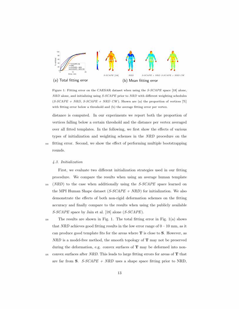
0 10 20

Error, mm

0

20

40

60

80

100

% v

ert

ices

S-SCAPE [18]

NRD

S-SCAPE + NRD

S-SCAPE + NRD CW

(a) Total fitting error

S-SCAPE [18] NRD S-SCAPE + NRD S-SCAPE + NRD CW

(b) Mean fitting error

Figure 1: Fitting error on the CAESAR dataset when using the S-SCAPE space [18] alone,

NRD alone, and initializing using S-SCAPE prior to NRD with different weighting schedules

(S-SCAPE + NRD, S-SCAPE + NRD CW ). Shown are (a) the proportion of vertices [%]

with fitting error below a threshold and (b) the average fitting error per vertex.

distance is computed. In our experiments we report both the proportion of

vertices falling below a certain threshold and the distance per vertex averaged

over all fitted templates. In the following, we first show the effects of various

types of initialization and weighting schemes in the NRD procedure on the

fitting error. Second, we show the effect of performing multiple bootstrapping310

rounds.

4.3. Initialization

First, we evaluate two different initialization strategies used in our fitting

procedure. We compare the results when using an average human template

(NRD) to the case when additionally using the S-SCAPE space learned on315

the MPI Human Shape dataset (S-SCAPE + NRD) for initialization. We also

demonstrate the effects of both non-rigid deformation schemes on the fitting

accuracy and finally compare to the results when using the publicly available

S-SCAPE space by Jain et al. [18] alone (S-SCAPE ).

The results are shown in Fig. 1. The total fitting error in Fig. 1(a) shows320

that NRD achieves good fitting results in the low error range of 0 – 10 mm, as it

can produce good template fits for the areas where T is close to S. However, as

NRD is a model-free method, the smooth topology of T may not be preserved

during the deformation, e.g. convex surfaces of T may be deformed into non-

convex surfaces after NRD. This leads to large fitting errors for areas of T that325

are far from S. S-SCAPE + NRD uses a shape space fitting prior to NRD,

13

which allows for a better initial alignment of T to S. Note that S-SCAPE +

NRD results in a better fitting accuracy in the high error range of 10− 20 mm.

The fitting result by S-SCAPE + NRD favorably compares against using S-

SCAPE alone. Although S-SCAPE results into deformations preserving the330

human body shape topology, the shape space is learned from the relatively

specialized MPI Human Shape dataset containing mostly young adults and thus

cannot represent all shape variations.

We also analyze the differences in the mean fitting errors per vertex in

Fig. 1(b). NRD achieves good fitting results for most of the vertices. How-335

ever, the arms are not fitted well due to differences in body posture of T and S.

Furthermore, the average fitting error is not smooth, which shows that despite

using Es, NRD may produce non-smooth deformations. In contrast, the result

of S-SCAPE + NRD is smoother and has a lower fitting error for the arms.

Clearly, the average fitting error of S-SCAPE is much higher, with notably340

worse fitting results for arms, belly and chest.

4.4. NRD parameters

Second, we evaluate the influence of the weight relaxation during NRD on the

fitting accuracy. Specifically, we compare the standard weighting scheme where

weights are relaxed in each iteration (S-SCAPE + NRD) to the case where the345

weights stay constant (S-SCAPE + NRD CW ). Fig. 1(a) shows that the total

fitting error of S-SCAPE + NRD is lower than S-SCAPE + NRD CW. This

is because S-SCAPE + NRD CW enforces higher localized rigidity by keeping

weights constantly high, while S-SCAPE + NRD relaxes the weights so that

T can fit more accurately to S. This explanation is supported by consistently350

higher per-vertex mean fitting errors in case of S-SCAPE + NRD CW compared

to S-SCAPE + NRD, as shown in Fig. 1(b). The highest differences are in the

areas of high body shape variability, such as belly and chest. Different weight

reduction schemes such as β := 0.5β, γ := 0.5γ and β := 0.25β, γ := 0.25γ lead

to better fitting accuracy compared to constant weights, with the latter scheme355

achieving slightly better results and faster convergence rates. We thus use the

14

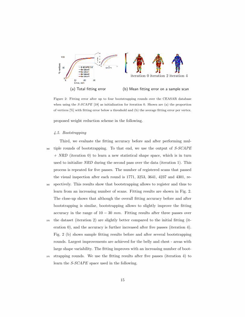
(a) Total fitting error

iteration 0 iteration 2 iteration 4

(b) Mean fitting error on a sample scan

Figure 2: Fitting error after up to four bootstrapping rounds over the CEASAR database

when using the S-SCAPE [18] as initialization for iteration 0. Shown are (a) the proportion

of vertices [%] with fitting error below a threshold and (b) the average fitting error per vertex.

proposed weight reduction scheme in the following.

4.5. Bootstrapping

Third, we evaluate the fitting accuracy before and after performing mul-

tiple rounds of bootstrapping. To that end, we use the output of S-SCAPE360

+ NRD (iteration 0) to learn a new statistical shape space, which is in turn

used to initialize NRD during the second pass over the data (iteration 1). This

process is repeated for five passes. The number of registered scans that passed

the visual inspection after each round is 1771, 3253, 3641, 4237 and 4301, re-

spectively. This results show that bootstrapping allows to register and thus to365

learn from an increasing number of scans. Fitting results are shown in Fig. 2.

The close-up shows that although the overall fitting accuracy before and after

bootstrapping is similar, bootstrapping allows to slightly improve the fitting

accuracy in the range of 10 − 30 mm. Fitting results after three passes over

the dataset (iteration 2) are slightly better compared to the initial fitting (it-370

eration 0), and the accuracy is further increased after five passes (iteration 4).

Fig. 2 (b) shows sample fitting results before and after several bootstrapping

rounds. Largest improvements are achieved for the belly and chest - areas with

large shape variability. The fitting improves with an increasing number of boot-

strapping rounds. We use the fitting results after five passes (iteration 4) to375

learn the S-SCAPE space used in the following.

15

5. Evaluation of statistical shape space

In this section, we evaluate the S-SCAPE space using the statistical quality

measures of generalization and specificity [31].

5.1. Quality measure380

We use two complementary measures of shape statistics. Generalization

evaluates the ability of a shape space to represent unseen instances of the object

class. Good generalization means the shape space is capable of learning the

characteristics of an object class from a limited number of training samples,

poor generalization indicates overfitting of the training set. Generalization is385

measured using leave-one-out cross reconstruction of training samples, i.e. the

shape space is learned using all but one training sample and the resulting shape

space is fitted to the excluded sample. The fitting error is measured using the

mean vertex-to-vertex Euclidean distance. Generalization is reported as mean

fitting error averaged over the complete set of trials, and plotted as a function390

of the number of shape space parameters. It is expected that the mean error

decreases until convergence as the number of shape space parameters increases.

Specificity measures the ability of a shape space to generate instances of the

object class that are similar to the training samples. The specificity test is per-

formed by generating a set of instances randomly drawn from the learned shape395

space and by comparing them to the training samples. The error is measured

as average distance of the generated instances to their nearest neighbors in the

training set. It is expected that the mean distance increases until convergence

with increasing number of shape space parameters. We follow Styner et al. [31]

and generate 10,000 random samples.400

5.2. Bootstrapping

We evaluate the influence of bootstrapping on the quality of the statisti-

cal shape space by comparing models obtained after zero, one, two and four

iterations of bootstrapping. The geometry of the training samples changes in

each bootstrapping round, which makes the generalization and specificity results405

16

Gen

era

lizati

on

1 5 10 15 20 25 300

5

10

15

20

25

# PCA coefficients

Dis

tan

ce

, m

m

iteration 0

iteration 1

iteration 2

iteration 4

1 5 10 15 20 25 300

5

10

15

20

25

# PCA coefficients

Dis

tan

ce

, m

m

train 50

train 100

train 1000

train 4307

1 5 10 15 20 25 300

5

10

15

20

25

# PCA coefficients

Dis

tan

ce

, m

m

none

normalization WSX

normalization NH

Sp

ecifi

cit

y

1 5 10 15 20 25 300

5

10

15

20

25

# PCA coefficients

Dis

tan

ce

, m

m

iteration 0

iteration 1

iteration 2

iteration 4

1 5 10 15 20 25 300

5

10

15

20

25

# PCA coefficients

Dis

tan

ce

, m

m

train 50

train 100

train 1000

train 4307

1 5 10 15 20 25 300

5

10

15

20

25

# PCA coefficients

Dis

tan

ce

, m

m

none

normalization WSX

normalization NH

(a) bootstrapping (b) # training samples (c) posture normalization

Figure 3: Influence of different design choices on statistical quality measures. Shown are

influence of (a) bootstrapping, (b) number of training samples and (c) posture normalization

on generalization (top row) and specificity (bottom row). Best viewed with zoom on the

screen.

incomparable across different shape spaces. We thus use the training samples

obtained after four iterations of bootstrapping as “ground truth”, i.e., the recon-

struction error of generalization and the nearest neighbor distance of specificity

for each shape space is computed w.r.t. fitting results after four bootstrap-

ping rounds. This allows for a fair comparison across different statistical shape410

spaces.

The results are shown in Fig. 3(a). Generalization error is already low after

a single iteration of bootstrapping because after one iteration, the shape space

is learned from a significantly larger number of training samples, thereby using

samples with higher shape variation that were discarded in the 0th iteration.415

The following rounds of bootstrapping have little influence on generalization

and specificity, with the shape space after four iterations resulting in a slightly

lower specificity error than for previous iterations for a small number of shape

parameters.

17

5.3. Number of training samples420

To evaluate the influence of the number of training samples, we vary the

number of samples obtained after four bootstrapping iterations. Specifically,

we consider subsets of 50, 100, 1, 000 and 4, 307 (all − 1) training samples.

To compute a shape space, the desired number of training shapes are sampled

from the entire set of training samples. For generalization, we cross-evaluate425

on all 4, 308 training samples by leaving one sample out and by sampling the

desired number of training shapes from the remaining samples. For specificity,

we compute the nearest-neighbor distances to all 4, 308 training samples to find

the closest sample.

The results are shown in Fig. 3(b). The shape space learned from the smallest430

number of samples performs worst. Increasing the number of samples consis-

tently improves the performance with the best results achieved when using the

maximum number. Both generalization and specificity error reduction is most

pronounced when increasing the number of samples from 50 to 100. Further in-

creasing the number of samples to 1, 000 affects specificity much stronger than435

generalization. This shows that the shape space learned from only 100 samples

generalizes well, while its generative qualities are poor. Increasing the number

of samples from 1, 000 to 4, 307 only slightly reduces both generalization and

specificity errors, which shows that a high-quality statistical shape space can be

learned from 1, 000 samples.440

5.4. Posture normalization

Finally, we evaluate the generalization and specificity of the shape space ob-

tained when performing posture normalization using the methods of Wuhrer et al.

[38] (WSX ) and Neophytou and Hilton [21] (NH ). The results are shown in

Fig. 3 (c). Posture normalization significantly improves generalization and445

specificity, with WSX achieving the best result. The reduction of the aver-

age fitting error in case of generalization is highest for a low number of shape

parameters. This is because both WSX and NH lead to shape spaces that are

18

more compact compared to the shape space obtained with unnormalized train-

ing shapes. Additionally, both posture-normalized shape spaces exhibit much450

better specificity. Compared to the shape space trained before posture nor-

malization, randomly generated samples from both shape spaces trained after

WSX and NH exhibit less variation in posture and are thus more similar to

their corresponding posture-normalized training samples.

Finally, we qualitatively examine the first five PCA components learned455

by the following S-SCAPE spaces: the current state-of-the-art shape space S-

SCAPE [18], our shape space without posture normalization and with posture

normalization using WSX and NH. The results are shown in Fig. 4. Major

modes of shape variation by S-SCAPE (row 1) are affected by global and local

posture-related deformations, such as moving of arms or tilting the body. In460

contrast, the principal modes of variation by our shape space (row 2) are mostly

due to shape changes, which is achieved due to better template fitting proce-

dure and a more representative training set. However, small posture variations

are still part of the learned shape space. Performing posture normalization of

the training samples prior to learning the shape space completely factors out465

changes due to posture, as can be seen in the major principal components of

ours+WSX (row 3) and ours+NH (row 4).

6. Human body reconstruction

Finally, we evaluate our improved S-SCAPE spaces on the task of estimating

human body shape from sparse and noisy visual input. We follow the approach470

by Helten et al. [17] to estimate the body shape of a person from two sequentially

taken front and back depth images. First, body shape and posture are fitted

independently to each depth image. Second, the obtained results are used as

initialization of a method that jointly optimizes over shape and independently

optimizes over posture parameters. This optimization strategy is used because475

the shape in both depth scans is of the same person, but the pose may differ.

19

S-S

CAPE

[18]

ours

ours

+W

SX

ours

+NH

st. dev. +3σ −3σ +3σ −3σ +3σ −3σ +3σ −3σ +3σ −3σ

PCA id I II III IV V

Figure 4: Visualization of the first five PCA eigenvectors scaled by ±3σ (standard deviation).

Shown are eigenvectors of the S-SCAPE space [18] (row 1) and the S-SCAPE spaces trained

using our pre-processed data without (row 2) and with posture normalization using WSX [38]

(row 3) and NH [21] (row 4).20

6.1. Dataset and experimental setup

We use a publicly available dataset [17] containing Kinect body scans of three

males and three females. Examples of the Kinect scans are shown in Fig. 6(a).

For each subject, a high-resolution laser scan was captured to determine “ground480

truth” body shape. Following the evaluation protocol of Helten et al. [17] we

first fit a shape space to the depth data, then fit shape space to the ground

truth scan, and finally compute the fitting error as a vertex-to-vertex Euclidean

distance between the vertices of the depth-fitted mesh and the ground truth-

fitted mesh. As the required landmarks are not available for this dataset, we485

manually placed 14 landmarks on each depth and laser scan.

6.2. Quantitative evaluation

For quantitative evaluation, we compare the following four shape models

presented above: the current state-of-the-art shape space [18], our shape space

without posture normalization and with posture normalization using WSX and490

NH. In our experiments, we vary the number of shape space parameters and

the number of training samples. To evaluate the fitting accuracy, we report the

proportion of vertices below a certain threshold.

The results are shown in Fig. 5, where the number of shape space parameters

varies in the columns and the number of training samples varies in the rows. In495

all cases our S-SCAPE spaces learned from the CAESAR dataset significantly

outperform the shape space by Jain et al., which is learned from the far less

representative MPI Human Shape dataset. Our models achieve good fitting ac-

curacy when using as few as 20 shape parameters, and the performance stays

stable when increasing the number of shape parameters up to 50 (first row). In500

contrast, the performance of the shape space by Jain et al. drops, possibly due

to overfitting to unrealistic shape deformations in noisy depth data. Interest-

ingly, better performance by our models is evident even in the case when all

models are learned from the same number of training samples (third and fourth

rows). This shows that the CAESAR data has higher shape variability than the505

MPI Human Shape data. In the majority of cases, the shape space learned from

21

# train # PCA coefficientssampl.

20 30 40 50all

0 10 20

Error, mm

0

50

100

% v

ert

ices

S-SCAPE [18]oursours + WSXours + NH

0 10 20

Error, mm

0

50

100

% v

ert

ices

S-SCAPE [18]oursours + WSXours + NH

0 10 20

Error, mm

0

50

100

% v

ert

ices

S-SCAPE [18]oursours + WSXours + NH

0 10 20

Error, mm

0

50

100

% v

ert

ices

S-SCAPE [18]oursours + WSXours + NH

1000

0 10 20

Error, mm

0

50

100

% v

ert

ices

ours

ours + WSX

ours + NH

0 10 20

Error, mm

0

50

100

% v

ert

ices

ours

ours + WSX

ours + NH

0 10 20

Error, mm

0

50

100

% v

ert

ices

ours

ours + WSX

ours + NH

0 10 20

Error, mm

0

50

100

% v

ert

ices

ours

ours + WSX

ours + NH

100

0 10 20

Error, mm

0

50

100

% v

ert

ices

S-SCAPE [18]oursours + WSXours + NH

0 10 20

Error, mm

0

50

100

% v

ert

ices

S-SCAPE [18]oursours + WSXours + NH

0 10 20

Error, mm

0

50

100

% v

ert

ices

S-SCAPE [18]oursours + WSXours + NH

0 10 20

Error, mm

0

50

100

% v

ert

ices

S-SCAPE [18]oursours + WSXours + NH

50

0 10 20

Error, mm

0

50

100

% v

ert

ices

S-SCAPE [18]oursours + WSXours + NH

0 10 20

Error, mm

0

50

100

% v

ert

ices

S-SCAPE [18]oursours + WSXours + NH

0 10 20

Error, mm

0

50

100%

vert

ices

S-SCAPE [18]oursours + WSXours + NH

Figure 5: Fitting error on the dataset of depth scans [17] of S-SCAPE spaces by Jain et

al. [18] and S-SCAPE spaces trained using our processed data without and with posture

normalization using WSX and NH. Shown is the proportion of vertices [%] for which the

fitting error falls below a threshold.

the posture-normalized samples with NH outperforms the shape space learned

from samples without posture normalization. This shows that the posture nor-

malization method of Neophytou and Hilton [21] helps to improve the accuracy

of fitting to noisy depth data. Surprisingly, the shape space learned from sam-510

ples without posture normalization outperforms the shape space learned from

the posture-normalized samples with WSX in most cases. Overall, the quanti-

tative results show the advantages of our approach of building S-SCAPE spaces

learned from a large representative set of training samples with additional pos-

ture normalization.515

22

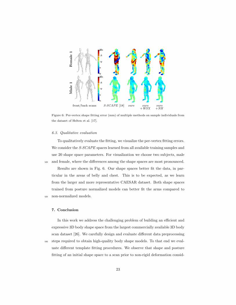
Female

1M

ale

1

front/back scans S-SCAPE [18] ours ours ours+WSX +NH

Figure 6: Per-vertex shape fitting error (mm) of multiple methods on sample individuals from

the dataset of Helten et al. [17].

6.3. Qualitative evaluation

To qualitatively evaluate the fitting, we visualize the per-vertex fitting errors.

We consider the S-SCAPE spaces learned from all available training samples and

use 20 shape space parameters. For visualization we choose two subjects, male

and female, where the differences among the shape spaces are most pronounced.520

Results are shown in Fig. 6. Our shape spaces better fit the data, in par-

ticular in the areas of belly and chest. This is to be expected, as we learn

from the larger and more representative CAESAR dataset. Both shape spaces

trained from posture normalized models can better fit the arms compared to

non-normalized models.525

7. Conclusion

In this work we address the challenging problem of building an efficient and

expressive 3D body shape space from the largest commercially available 3D body

scan dataset [26]. We carefully design and evaluate different data preprocessing

steps required to obtain high-quality body shape models. To that end we eval-530

uate different template fitting procedures. We observe that shape and posture

fitting of an initial shape space to a scan prior to non-rigid deformation consid-

23

erably improves the fitting results. Our findings indicate that multiple passes

over the dataset improve initialization and thus increase the overall fitting ac-

curacy and statistical shape space qualities. Furthermore, we show that posture535

normalization prior to learning a shape space leads to significantly better gen-

eralization and specificity of the S-SCAPE spaces. Finally, we demonstrate the

advantages of our learned shape spaces over the state-of-the-art shape space of

Jain et al. [18] learned on largest publicly available dataset [16] on the task of

human body shape reconstruction from noisy depth data.540

We release our S-SCAPE spaces, registered CAESAR scans, raw scan pre-

processing code, code to fit a S-SCAPE space to a raw scan and evaluation code

for public usage1. We believe this contribution is required for future develop-

ment in human body modeling.

Acknowledgements545

We thank Alexandros Neophytou and Adrian Hilton for sharing their posture

normalization code. This work was partially funded by the Cluster of Excellence

MMCI.

References

[1] B. Allen, B. Curless, and Z. Popovic. The space of human body shapes: recon-550

struction and parameterization from range scans. TG’03.

[2] B. Allen, B. Curless, Z. Popovic, and A. Hertzmann. Learning a correlated model

of identity and pose-dependent body shape variation for real-time synthesis. In

SCA’06.

[3] D. Anguelov, P. Srinivasan, D. Koller, S. Thrun, J. Rodgers, and J. Davis.555

SCAPE: shape completion and animation of people. TG’05.

[4] S.-Y. Baek and K. Lee. Parametric human body shape modeling framework for

human-centered product design. CAD’12.

1Available at http: // humanshape. mpi-inf. mpg. de

24

[5] A. Balan and M. Black. The naked truth: Estimating body shape under clothing.

In ECCV’08.560

[6] A. Balan, L. Sigal, M. Black, J. Davis, and H. Haussecker. Detailed human shape

and pose from images. In CVPR’07.

[7] F. Bogo, J. Romero, M. Loper, and M. Black. FAUST: Dataset and evaluation

for 3D mesh registration. In CVPR’14.

[8] J. Boisvert, C. Shu, S. Wuhrer, and P. Xi. Three-dimensional human shape565

inference from silhouettes: Reconstruction and validation. MVAP’13.

[9] Y. Chen, Z. Liu, and Z. Zhang. Tensor-based human body modeling. In CVPR’13.

[10] C.-H. Chu, Y.-T. Tsai, C. Wang, and T.-H. Kwok. Exemplar-based statistical

model for semantic parametric design of human body. Comp. in Ind.’10.

[11] C. Goodall. Procrustes Methods in the Statistical Analysis of Shape. J. R. Stat.570

Soc. Ser. B Stat. Methodol.’91.

[12] P. Guan, L. Reiss, D. Hirshberg, A. Weiss, and M. Black. DRAPE: DRessing

Any PErson. TG’12.

[13] P. Guan, A. Weiss, A. Balan, and M. Black. Estimating human shape and pose

from a single image. In ICCV’09.575

[14] N. Hasler, H. Ackermann, B. Rosenhahn, T. Thormahlen, and H.-P. Seidel. Mul-

tilinear pose and body shape estimation of dressed subjects from image sets. In

CVPR’10.

[15] N. Hasler, C. Stoll, B. Rosenhahn, T. Thormahlen, and H.-P. Seidel. Estimating

body shape of dressed humans. Comput. & Graph.’09.580

[16] N. Hasler, C. Stoll, M. Sunkel, B. Rosenhahn, and H.-P. Seidel. A statistical

model of human pose and body shape. CGF’09.

[17] T. Helten, A. Baak, G. Bharai, M. Muller, H.-P. Seidel, and C. Theobalt. Person-

alization and evaluation of a real-time depth-based full body scanner. In 3DV’13.

[18] A. Jain, T. Thormahlen, H.-P. Seidel, and C. Theobalt. MovieReshape: tracking585

and reshaping of humans in videos. TG’10.

25

[19] Matthew Loper, Naureen Mahmood, Javier Romero, Gerard Pons-Moll, and

Michael Black. Smpl: A skinned multi-person linear model. TG’15.

[20] L. Mundermann, S. Corazza, and T. Andriacchi. Accurately measuring human

movement using articulated icp with soft-joint constraints and a repository of590

articulated models. In CVPR’07.

[21] A. Neophytou and A. Hilton. Shape and pose space deformation for subject

specific animation. In 3DV’13.

[22] T. Neumann, K. Varanasi, N. Hasler, M. Wacker, M. Magnor, and C. Theobalt.

Capture and statistical modeling of arm-muscle deformations. CGF’13.595

[23] L. Pishchulin, A. Jain, M. Andriluka, T. Thormahlen, and B. Schiele. Articulated

people detection and pose estimation: Reshaping the future. In CVPR’12.

[24] L. Pishchulin, A. Jain, C. Wojek, T. Thormaehlen, and B. Schiele. In good shape:

Robust people detection based on appearance and shape. In BMVC’11.

[25] Gerard Pons-Moll, Javier Romero, Naureen Mahmood, and Michael Black.600

DYNA: a model of dynamic human shape in motion. TG’15.

[26] K. Robinette, H. Daanen, and E. Paquet. The CAESAR project: A 3-D surface

anthropometry survey. In 3DIM’99.

[27] C. Rupprecht, O. Pauly, C. Theobalt, and S. Ilic. 3d semantic parameterization

for human shape modeling: Application to 3d animation. In 3DV’13.605

[28] H. Seo and N. Magnenat-Thalmann. An automatic modeling of human bodies

from sizing parameters. In I3D ’03.

[29] H. Seo, Y. In Yeo, and K. Wohn. 3D body reconstruction from photos based on

range scan. In Edutainment’06.

[30] L. Sigal, A. Balan, and M. Black. Combined discriminative and generative artic-610

ulated pose and non-rigid shape estimation. In NIPS’07.

[31] M. Styner, K. Rajamani, L.-P. Nolte, G. Zsemlye, G. Szekely, C. Taylor, and

R. Davies. Evaluation of 3D correspondence methods for model building. In

IPMI’03.

26

[32] G. Tam, Z.-Q. Cheng, Y.-K. Lai, F. Langbein, Y. Liu, D. Marshall, R. Martin,615

X.-F. Sun, and P. Rosin. Registration of 3D point clouds and meshes: A survey

from rigid to non-rigid. TVCG’13.

[33] Aggeliki Tsoli, Naureen Mahmood, and Michael Black. Breathing life into shape:

Capturing, modeling and animating 3d human breathing. TG’14.

[34] O. van Kaick, H. Zhang, G. Hamarneh, and D. Cohen-Or. A survey on shape620

correspondence. CGF’11.

[35] A. Weiss, D. Hirshberg, and M. Black. Home 3D body scans from noisy image

and range data. In ICCV’11.

[36] S. Wuhrer and C. Shu. Estimating 3d human shapes from measurements.

MVAP’13.625

[37] S. Wuhrer, C. Shu, and P. Xi. Landmark-free posture invariant human shape

correspondence. The Vis. Comput.’11.

[38] S. Wuhrer, C. Shu, and P. Xi. Posture-invariant statistical shape analysis using

Laplace operator. Comput. & Graph.’12.

[39] Stefanie Wuhrer, Leonid Pishchulin, Alan Brunton, Chang Shu, and Jochen Lang.630

Estimation of human body shape and posture under clothing. CVIU’14.

[40] P. Xi, W.-S. Lee, and C. Shu. A data-driven approach to human-body cloning

using a segmented body database. In PG’07.

[41] S. Zhou, H. Fu, L. Liu, D. Cohen-Or, and X. Han. Parametric reshaping of human

bodies in images. TG’10.635

[42] C. Zhu, R. Byrd, P. Lu, and J. Nocedal. Algorithm 778: L-BFGS-B Fortran

subroutines for large-scale bound-constrained optimization. TOMS’97.

27