Is Trade Facilitation The Right Direction To Go In

Building Trade Capacity?

Jennifer Wing Shan Yuen

B.Sc., University of British Columbia, 2004

RESEARCH PROJECT SUBMITTED IN PARTIAL FULFILLMENT

OF THE REQUIREMENTS FOR THE DEGREE OF

MASTER OF ARTS

in the Department

of

Economics

O Jennifer Yuen 2005

SIMON FRASER UNIVERSITY

Fall 2005

All rights reserved. This work may not be

reproduced in whole or in parts, by photocopy

or other means, without permission of the author.

APPROVAL

Name: Jennifer Yuen

Degree: M. A. (Economics)

Title of Project : Is Trade Facilitation The Right Direction To Go In Building Trade Capacity?

Examining Committee :

Chair: Brian Krauth

Steve Easton Senior Supervisor

David Jacks Supervisor

Terry Heaps Internal Examiner

Date Approved: Thursday, December 1,2005

. . 11

SIMON FRASER UNIVERSIW~~ brary

DECLARATION OF PARTIAL COPYRIGHT LICENCE

The author, whose copyright is declared on the title page of this work, has granted to Simon Fraser University the right to lend this thesis, project or extended essay to users of the Simon Fraser University Library, and to make partial or single copies only for such users or in response to a request from the library of any other university, or other educational institution, on its own behalf or for one of its users.

The author has further granted permission to Simon Fraser University to keep or make a digital copy for use in its circulating collection, and, without changing the content, to translate the thesislproject or extended essays, if technically possible, to any medium or format for the purpose of preservation of the digital work.

The author has further agreed that permission for multiple copying of this work for scholarly purposes may be granted by either the author or the Dean of Graduate Studies.

It is understood that copying or publication of this work for financial gain shall not be allowed without the author's written permission.

Permission for public performance, or limited permission for private scholarly use, of any multimedia materials forming part of this work, may have been granted by the author. This information may be found on the separately catalogued multimedia material and in the signed Partial Copyright Licence.

The original Partial Copyright Licence attesting to these terms, and signed by this author, may be found in the original bound copy of this work, retained in the Simon Fraser University Archive.

Simon Fraser University Library Burnaby, BC, Canada

ABSTRACT

This paper uses the gravity equation of international trade to study the relationship

between trade facilitation commitments and trade flows using the OECDIWTO Trade

Capacity Building - Trade Facilitation Database. In the analyses of 257 donor-recipients

pairs, it is found that bilateral trade facilitation commitments are positively related, while

multilateral sources are negatively related to exports from recipients to donors. These

negative relationships for the multilateral institutions were found by using cross-sectional

studies and are significant, for all but the World Customs Organization. From the first-

differenced estimations, changes in exports from recipients to donors covariate positively

with changes in the World Customs Organization trade facilitation commitments; the

estimated effect is 0.23 percent to 0.41 percent increase in exports for every 10 percent

increase in the World Customs Organization trade facilitation commitments. There is no

evidence that changes in other trade facilitation sources will bring significant changes to

bilateral trade.

Keywords: trade facilitation, gravity model, capacity building

DEDICATION

Gis paper is dedicated to my parents for their sacn$ices,

unconditionalsupport andlove throughout my academic career.

ACKNOWLEGDEMENT

I would like to thank my Advisory Committee members, Dr. Stephen Easton, Dr.

David Jacks and Dr. Terry Heaps for their guidance.

I am grateful to Dr. Jane Friesen and Dr. Krishna Pendakur, who gave me

invaluable advice during my graduate study.

I would also like to express my gratitude to Mr. Yuen Pau Woo and Mr. Nizar

Assanie at the Asia Pacific Foundation of Canada for their inspiring introduction to the

research in trade facilitation.

TABLE OF CONTENTS

Approval

Abstract

Dedication

Acknowledgement

Table of Contents

List of Tables

List of Figures

Acronyms 1 Abbreviations

1. Introduction

2. Background on International Trade - Theories and Empirics

2.1. International Trade Theory

2.2. Gravity Model

2.2.1. History of the Gravity Model

2.2.2. Theoretical Framework for the Gravity Model

2.2.3. Applications of the Gravity Model

3. Data and Exploratory Analysis

4. Empirical Strategies

5. Empirical Results

5.1 Cross-Sectional Regression

5.2 First-Differenced Estimations

6. Future Research

7. Conclusion

Annex - Detailed Derivation of the Gravity Equation

Appendix

Bibliography

v

vi

vii . . .

V l l l

ix

1

5

5

6

7

9

12

19

24

28

28

3 3

37

3 8

3 9

4 2

5 5

LIST OF TABLES

Table 1. Distribution of Trade Facilitation Commitments by Donor Type

Table 2. Distribution of Trade Facilitation Commitments by Year

Table 3. Distribution of Trade Facilitation Commitments by Income Group and Year

Table 4. Distribution of Trade Facilitation Commitments by Region Group and Year

Table 5. Distribution of Funds to Recipients by Year

Table 6. Region of Trade Facilitation Concentration of Major Bilateral Donors

Table 7. Region of Trade Facilitation Concentration of Major Multilateral Donors

Table 8: Cross-Sectional Regression - Standard Gravity Model

Table 9a. Cross-sectional Regression - Trade Facilitation Variables

Table 9b. Cross-sectional Regression - Trade Facilitation Variables

Table 10. Cross-Sectional Regression - Weighted Least Squares

Table 1 1 . Cross-sectional Regression - based on different units of account

Table 12. First-differenced estimation - with 1 -year gap

Table 13. First-differenced estimation - with 5-year gap

vii

LIST OF FIGURES

Figure 1. Trade Facilitation Commitments from Different Donor Type 42

Figure 2. Trade Facilitation Commitments by Year 42

Figure 3. Trade Facilitation Commitments from Different Donor Type 43

Figure 4. Distribution of Funds by Year 4 5

Figure 5. Region of Trade Facilitation Concentration of Major Bilateral Donors 46

Figure 6. Region of Trade Facilitation Concentration of Major Multilateral Donors 47

. . . V l l l

ACRONYMS / ABBREVIATIONS

All TF

APEC

CE

CEECINIS

EB

EU

HICs

LAIA

LAS

LDCs

LICs

LIMCs

PE

RE

TF All Bi

TF All Multi

TF Bi (D-to-R)

TF EC

TF Other Bi

TF Other Multi

TF UN

TF WCO

TF WTO

Trade facilitation commitments from all bilateral and multilateral donors

Asia-Pacific Economic Cooperation

Customs environment

Central and Eastern European Countries and the Newly Independent

States of the Former Soviet Union

E-business usage

European Union

High income countries

Latin American Integration Association

League of Arab States

Least developed countries

Low income countries

Lower middle income countries

Port efficiency

Regulatory environment

Trade facilitation commitments from all bilateral donors

Trade facilitation commitments from all multilateral donors

Trade facilitation commitments between specific pair of donor and

recipient

Trade facilitation commitments from the European Commission

Trade facilitation commitments from all bilateral donors minus trade

facilitation commitments between specific pair of donor and recipient

Trade facilitation commitments from multilateral agencies other than the

EC, UN, WCO and WCO

Trade facilitation commitments from the United Nations

Trade facilitation commitments from the World Customs Organization

Trade facilitation commitments from the World Trade Organization

1. Introduction

International trade has become an integral part of most countries' everyday

activities. For the communist countries that once operated closed economies, their

markets have gradually opened up to foreigners. The best examples are China and the

Former Soviet Union states. In recent years, China and the Eastern European countries

are some of the fastest-growing economies in the world. According to the Pacific

Economic Cooperation Council publication - the 2005-2006 Pacific Economic Outlook,

China is expected to have an annual Gross Domestic Product (GDP) growth of about 8%

in 2005 and 2006. This growth rate is predicted to be sustained for the next decade. The

potentials of these economies are hard to project because there is still a lot to be learned

about these new open economies. The disappearance of autarkic economies is no

surprise because there is a net gain from trade, and it is possible to make all players better

off by enlarging each player's consumption level.

As these countries and other emerging economies enter the world of international

trade, there are many international rules and regulations with which they need to comply.

While these countries are enjoying a higher living standard, there are also many other

economies that have been stagnating for a long period of time. Examples are the least

developed countries (LDCs) and the low income countries (LICs) in Africa and South

Asia. Some of these stagnations may be attributed to political or social instability that

makes doing businesses risky, or other man-made or natural disasters that destroy

infrastructure. For example, Afghanistan has been in wars for many years. These wars

not only create physical damages to the country, but also create an unsafe image for the

country. Without a secure and infrastructure equipped economy, these countries can

hardly attract investors. Another possible reason for not engaging in trading is that most

goods produced by these LDCs and LICs, such as agricultural and manufacturing

products, face high tariff rates. However, as reported by various organizations,

procedural impediments can serve as stronger barriers to trade than tariffs in developing

countries.' This can be good news for these stagnant economies. Even if developed

' APFC and The World Bank, Cutting Through Red Tape: New Directions for APEC's Trade Facilitation Agenda, (Novemeber 2000)

economies that use the tariff to protect their low-end industries may not easily reduce

tariffs, the LDCs and LICs can still unilaterally reduce trade barriers by eliminating their

own procedural impediments to trade. The lack of a trade facilitation structure also

makes the potential gains of commitments to such an area high.

To build trade capacity, many multilateral trade institutions provide assistance of

various forms to countries in transition, the LDCs and LICs. To trade internationally,

there are internationally set rules and regulations to follow. Raising the standards of

developing countries to meet international regulations can be considered as a trade

facilitating procedure. Building the necessary infrastructure for transportation and

communication can also be viewed as trade facilitating. Since it is a new area of research,

there is no formal or universally-agreed definition of trade facilitation. Definitions used

by some multilateral agencies can be found in Wilson, Mann and Otsuki (WMO) 2003.

Trade facilitation is also a new item on the World Trade Organization (WTO) Ministerial

Conference Agenda. It was first introduced as a separate entity for negotiations in the

1996 WTO Ministerial Conference at Singapore. According to the Organization for

Economic Cooperation and Development (OECD) and the World Trade Organization

(WTO) in 2005, the definition of trade facilitation is the "simplification and

harmonization of international trade procedures related to the movement of goods across

borders". "Trade procedures include the activities, practices and formalities involved in

collecting, presenting, communicating and processing data and other information

required for the movement of goods in international trade."

More concretely, trade facilitation has been characterized by four areas of interest:

port efficiency, customs environment, regulatory environment and service-sector

infrastructure. Port efficiency addresses Article V of the General Agreement on Tariffs

and Trade (GATT) - freedom of transit. Article V says that "freedom of movement

through the territory of each contracting party is to be assured for goods (and their

conveyances), which are destined to or come from any other contracting party. Such

traffic must be allowed to move via the most convenient route; is to be exempted from

Joint WTO/OECD Trade Capacity Building Database - 2005 Data Collection

customs or transit duties; and is to be free from unnecessary delays or restriction^."^ The

customs environment corresponds to GATT Article VIII - fees and formalities connected

with importation and exportation. "Article VIII establishes that all fees and charges

(other than duties) imposed on, or in connection with, import or export shall be limited to

the approximate cost of services rendered, and shall not constitute indirect protection to

domestic products or taxation for fiscal purposes."4 The regulatory environment is

related to GATT Article X - publication and administration of trade regulations. "Article

X establishes two principles: First, all laws and regulations, judicial decisions and

administrative rulings, etc., affecting imports and exports should be published;

furthermore, they may not be enforced before official publication. Second, administration

of these laws, regulations, etc., shall be uniform, impartial and rea~onable."~

After 9 years of exploration, formulation and implementation in the area of trade

facilitation, the preliminary results of international commitments to trade facilitation will

be presented in the upcoming 6th WTO Ministerial Conference in Hong Kong (December

2005). The emerging attention to trade facilitation can be seen from the 197% (from 104

million USD to 309 million USD) increase in international commitments in this area

between 2001 and 2003. This trend continues in 2004. With only partial 2004 data

available as of October 2005, total commitment to trade facilitation sum to 343 million

USD in 2004, which is over the total in 2003. These values are computed using the

Trade Capacity Building - Trade Facilitation at abase^ launched jointly by the OECD

and the WTO in November 2002. This database is constructed based on the trade

facilitation definition given above, and it contains all commitments to trade facilitation

from both bilateral and multilateral sources to recipients between 2001 and 2003 and

partial commitments in 2004. This project also uses this Trade Facilitation Database to

study the research question: Is trade facilitation the right direction to go in building trade

Institute for Trade & Commercial Diplomacy at http://www.commerciaIdiplomacy.org/dictionaries.htm

WTO at http://ww.wto.org/english/thewto~e/whatis~e/eol/e/wtoO2/wto2~lO.htm

WTO at http://ww.wto.org/english/thewto:/whatise/eol/e/wtoO2/wto2IO.htm

6~oint WTOJOECD Trade Capacity Building Database Category 33 121 - 2005 Data Collection at hnp://tcbdb.wto.org.

capacity? More specifically, would trade volume increase with trade facilitation

commitments?

I propose using the gravity model, that is frequently used in studying bilateral

trade, to test the hypothesis that trade facilitation projects can enhance trade between the

country receiving and the country contributing to the building of trade capacity in the

area of trade facilitation. The modified gravity model attempts to account for the

variation in the bilateral trade flows by using trade facilitation contributions as an

explanatory variable in addition to the classic variables in the gravity model such as

distance between two countries, their GDP levels in actual value and in per capita terms,

tariff levels, trade preferential arrangements and language barriers. My first set of

regressions looks at the aggregate effects by using cross-sectional data, and my second

set of regressions uses the panel feature of the data to look at the before and after effect

and to accommodate the possibility of lagged response of trade flows to trade facilitation

commitments.

Another feature of this data set is that, multilateral institutions are involved in

about half of the records. Therefore, this gives an opportunity to examine the role of

multilateral donors on bilateral trade flows. This report should provide a better insight

about the significance of trade facilitation on trade than the previous works in this area

because previous works used computed indices to proxy trade facilitation levels while

this report employs real data to indicate improvement in trade facilitation.

The remainder of this paper is structured as follows: section 2 gives the history,

derivation and the previous uses of the gravity model; section 3 introduces the trade

facilitation data set; section 4 provides the framework for analyzing the trade facilitation

data; section 5 reports and discusses the statistical findings; section 6 discusses the issues

for future research; section 7 concludes.

2. Background on International Trade - Theories and Empirics

2.1 International Trade Theory

This report studies the relationship between trade flows and trade facilitation

commitments. Trade facilitation commitments can be viewed as aid from various sources

to improve trading environment in a recipient country. With these improvements, it is

believed that trade flows will increase. In order to justify such belief, it is necessary to

understand what the determinants of trade are. Theoretically, there are many factors that

potentially shape the pattern of international trade. There are three major schools of

thoughts regarding the three central questions in international trade: Why is there trade?

Who would trade? And what is being traded?

Using the fundamental supply and demand model, the three doctrines model the

demand side similarly as the aggregation of consumer preference from all over the world

for different goods; however, their theories on the supply side differ. Among the three

doctrines, the trade theory that has the longest history was developed by Ricardo in the

early nineteenth century. The Ricardian trade model was based on the concept that

relative cost differences among goods across countries arose from differences in the

technology of production. In essence, if a country has a comparative advantage in the

production of a commodity, it will produce and export this commodity until she reaches

her capacity. Since this methodology relies on comparative advantage and not on

absolute advantage, every country would produce at least one good according to the

Ricardian model. Together with the supply and demand framework at the world level, as

well as the domestic budget constraint -total income equals total expenditure - for each

country, consumption and production decisions for each commodity are made

simultaneously.

Another widely-adopted international trade model is the Heckscher-Ohlin model

postulated by Heckscher and Ohlin in the 1930s. This model uses relative factor

endowments to study the above three questions. Assuming that production of all goods

requires only two factors of production - labour and capital, the pattern of international

trade would be determined by the relative endowment of these factors as well as the

production technology of each good in each country. In other words, relatively labour-

intensity commodities tend to be produced or exported from countries with relatively

high labour-capital ratio.

The third type of model used to answer the three questions is essentially an

extension of the Heckscher-Ohlin model, the specific factor model. This allows for the

use of specific factors in various industries. For instance, all industries need labour as

input, but not all industries rely on both capital and land -the specific factors. Using the

Heckscher-Ohlin model argument, international trade pattern in the specific factor case

would also be driven by the relative endowment of each type of specific factors.

From the theoretical point of view, these three models are equally popular in the

field of international trade as they all have their own merits and are likely to shape trade

pattern jointly. Empirically, the trade pattern - bilateral trade in particular - is studied

extensively using the gravity model (Oguledo and MacPhee 1994).

2.2 Gravity Model

The gravity model earned its popularity in the study of bilateral trade flows since

the 1960s after Tinbergen (l962), Poyhonen and Pulliainen (1963) and Linnemann (1966)

applied such model to study trade pattern. The simplest form of the gravity model is:

& = (YJpl (17Pz(~0jp3 UV ... ... ... (la), or in logarithmic form:

ln(X,) = b,+Pl ln(YJ+P' ln(q)+PJ ln(Dil)+ ln(u,l) ... ... .. . (I b),

where X,, is the value of the flow from country i to country j, Yi (Y,) is the GDP in i (j),

Dl, is the distance between i and j, u,, is a log-normally distributed error term (In uij - N(O,o,)), and the p's tell how trade flow and GDPs and distance are linked. It is believed

and proven that GDPs are positively related, while distance is negatively related to trade

flow. This belief first arose from an analogy with the gravity theory in physics, which

states that the attraction between two masses grows as their masses increase and as the

distance between them decreases. Because of this non-economic explanation, the gravity

model has long been criticized. However, due to its high explanatory power, the model

has continued to be one of the most frequently used tools to study trade patterns by

researchers at all times. Today, the use of such model is subject to less criticism because

several economists like Anderson (1 979) and Bergstrand (1 985, 1989) built the gravity

model based on economic models, and thus provided a more rigorous economic basis for

the use and interpretation of the gravity model.

The rest of this section will present the history of the gravity model, followed by

the theoretical framework for it, and then finally the various applications of the model,

namely, preferential trade agreements, border effects and trade capacity assessments.

2.2.1 History of the Gravity Model

As early as the 1850s, the gravity model was used in social science studies of

human interactions such as the pattern of migration. In the 1940s, economists and

geographers started to recognize that there were potential benefits of collaborating with

each other to their respective studies. A simple but relevant example, the Heckscher-

Ohlin model requires knowledge about variation in endowment of different countries;

geographers would be a good resource. The field "Economic Geography" or "Space

Economy" was born, and "location theory" emerged. In 1954, Isard and Peck illustrated

diagrammatically that trade flow and distance, and thus transport costs, are negatively

related for both intra-national and international trade. They also provided an example

that uses the traditional opportunity cost and comparative advantage concepts to show the

direct relevance of relative geography due to the existence of transport costs in

determining production location and trade pattern. In that same year, Isard outlined an

"input-output analysis", which essentially modelled how national income is derived

through the interaction of input and output markets in a multi-country and multi-

commodity world. He then proposed the following trade-like relationship, which closely

resembles the gravity model presented above.

i V , = k Y, /Dva ... ... ... (21,

where iVj is the "income potential produced by nation j upon nation in, Yi is the "income

of nation j", Dii is the "average effective distance between nation i and j", k is "a constant

similar to the gravitational constant", and a is "a constant power to which Dii is raised".

Motivated by Isard and Peck's idea, Beckerman (1956) posed the research

question: "What is the importance of distance in determining the pattern of Western

European trade?" He reached 4 major conclusions using summary statistics; countries

near to one another traded markedly more, this was especially true for the less developed

nations in Europe whose degree of diversity in terms of trading partner was relatively low;

this tendency was less strong when three rather than two most important trade partners

are considered; both exports and imports showed similar tendency; such tendency did not

decline throughout the periods under study. He also made the following two inspiring

points. "Since one country's imports are another country's exports the actual distribution

of the first country's imports will depend on a mixture of two distance elements: (i) the

relative distance of every other country to the given country, which will influence the

import pattern of the given country in one way; and (ii) the relative distance of the given

country to each other country, which will affect the export pattern of each other country

and will thereby also have an effect on the import pattern of the given country." There

may also exist "psychic distance", such as a language barrier. Therefore, one may need

to consider concepts beyond physical bilateral distance to evaluate trade impediments.

The study of the distance term in the gravity model did not stop. Moneta ( 1 959)

found generally that the ratio of transportation cost to total cost of a commodity moves

inversely with its value per ton. This finding is worth-noting because underdeveloped

countries "are likely to trade low-valued commodities for high-valued commodity from"

industrialized countries. The relatively high transport costs of the low-valued

commodities could inhibit exports from the underdeveloped countries. This point on

relatively high transport costs on underdeveloped countries' exports was echoed by

Finger and Yeats (1976) in their study of the magnitudes of various trade protection

measures. They found that the protection by transport costs is more than equal to the

protection by tariffs. The implication therefore is that due to the nature of commodities

exported by underdeveloped countries, even if the tariffs against these countries are low,

exports may not significantly improve given the transport costs obstacle. Geraci and

Prewo (1977) also extended the study on transport cost, noting that the commodity

composition flowing between two countries is different in each direction. This suggests

that using distance as a proxy for transport cost for both directions is inadequate in a

pooling regression.

Year 1962 marked the first debut of the basic gravity model shown in equation (1).

Tinbergen proposed using this model to study the structure of world trade. In fact, he

also augmented the model with the Commonwealth and Benelux preferences dummies

and the difference in agriculture land per capita (a proxy for endowment) to capture their

effects on trade volume. In running the regression model for the 1958 bilateral world

trade data, he found that all the regressors were statistically significant with their

expected signs, and the explanatory power of the model was strikingly high, with the

unadjusted R* being 0.84. Due to these encouraging results, many researchers followed

suit even though there was no rigorous economic framework behind the use of the gravity

model. Linnemann (1966) further developed the basic gravity model proposed by

Tinbergen to a form that is used most often nowadays.

4 = f i (YJP1 ( v P 2 ( ~ 3 ~ ~ ( 4 j P 4 ( D ~ ~ ~ ~ u ~ ... ... ... (34, or in logarithmic form:

ln(Xj) = b,+PI 1n(YJ+f12 ln(I;)+P3 ln(NJ+P4 1n(NJ)+P5 ln(D,S + In@,,) ... (3b),

where the interpretations are the same as in equation (1) for the common terms, and N,

(N,) is the population of nation i 6). In his study, as well as many other studies,

population sizes have significant negative effect on trade flows. The economic intuition

behind the sign of each explanatory variable will be discussed in more details in later

sections. Similar to Tinbergen's model, Linnemann augmented his newly developed

gravity model with three trade preferences, namely the Commonwealth, French and

Belgian preferences. Again, Linnemann's model provided good fit for his 1958-1960

trade data, with all variables being statistically significant.

The gravity model had been used for more than a decade without any economic

theories behind it; the next section will provide three economic derivations of this model.

2.2.2 Theoretical Framework for the Gravity Model

Anderson (1979) was the first one to provide a theoretical foundation for the

gravity equation. A detailed derivation of the gravity model by Anderson can be found in

the Annex. His derivation of the gravity model was based on the properties of the

expenditure systems (basically income must equal sales) and the following assumptions

in the perfect competition setting. His main assumptions used to derive the simplest form

of the gravity equation include identical homothetic Cobb-Douglas preferences in all

countries (which give rise to identical expenditure functions), products are differentiated

by place of origin as each country is completely specialized, and tariffs and transport

costs are absent. By using a pure-expenditure system model, he found the following

relationship: X, = ,!% (K)" (I;)" His argument was that each country spends the same

portion of its income on country i's product (b,). Thus, the imports of good i by country j

is: X, = b,Y, . Country i's income equals to its sales: Y, = b,CI;. Thus, X, = Y,Y,/CI;

More realistically, he introduced a non-traded good sector, and assumed that

traded and non-traded goods are weakly separable in the utility function such that the

share of total trade expenditure of traded goods, with homotheticity, depends on traded

goods prices only. For the importing country j, let 8, be the share of j ' s expenditure on

country i's tradeable good divided by total expenditure in j on tradeables and 4, be the

share of expenditure on all tradeables in total expenditure of country j. Then, j's demand

for i's tradeables is given by: X, = 0, gl, I; , with the trade balance equation:

4, Y , = 0, (C, gl, I;). By imposing:

h = Fl(Y,, NJ = cm (Y,) )"I (NJaZ . . . . . . (4a), and

= F,(Y,, 4 ) = ,!% &)" . . . . . . (4b),

the gravity model becomes:

& = ko ( v ' (N,) (I;)" (4)" U , . . . . . . . . . (5a), or in logarithmic form:

h ( x J ) = k ~ + a ~ l n ( Y , ) + a ~ l n ( N , ) + ~ ~ In(I;)+pz In(N,)+h(u, ......... (5b).

Distance can easily be added to reflect transport costs. Assume that with transport costs

T,, the value of exports from i to j becomes X, T, instead ofx, , then j's demand for i's

tradeables becomes X, T,= T, 0, gl, I; , then the trade balance equation becomes: 4, Y , / T,

= 0, (C, gl, Y,/T,). Using distance as a proxy for transport costs:

T, = k2 dVS0 ... ... ... (6) ,

the gravity model becomes just like the one proposed by Linnemann (1 966):

X, = ko (Y,))"' (NJ)"' (I;)Pf p,)" (d,$ ' I uii .. . .. . . . . (74 , or in logarithmic form:

1n(Xj) = kl+a~ln(Y,)+azln~J+p~ln(I;)+pz lnpJ)+ 6rln(dij)+ln(~S ... ... (7b).

Noting that Y/N = y, where y is the real per capita income, the gravity model can be re-

written as:

......... x,] = yo (YJ" (y3" (yjjy3 (yJ) " (d,) ' u,, (7c), or in logarithmic form:

W X J ) = Y O O + Y I ~ ~ ( K ) + Y Z ~ ~ ( ~ J + Y ~ ~ ~ ( Y I ; ) + Y ~ 1n(yJ)+ yfWd,)+WuJ ..... (74 ,

This summarizes the work by Anderson. In fact, a slight variation of Anderson's

derivation was used by Thursby and Thursby (1987) and Oguledo and MacPhee (1 994) to

incorporate price levels of i and j as well as tariff rates between i and j. These can be

done through modifying conditions (4a), (4b) and (6) to:

= F, (Y,, N,, P3 = ao (YJ (N,) (P,) ......... ( w ,

......... 4 = Fl(yj, 4, PI) = f i ((I;" wJ)" (P~)'~ (8b), and

......... T, = kz d," ( I +t , f2 (9), respectively,

where PI (Pj) is country i's (j's) general price level, and tIJ is the ad valorem tariff imposed

by j on i's imports, and TIJ should now be interpreted as the trade barrier or trade cost

function as it no longer just reflects the transportation cost associated with trade. The

gravity models (7a) and (7b) then become:

X j = k4 (YJ (NJ (PJ a3 (YJ" fl)" (pJ)lM (d,,) '3 (1 + t,)" U , ......... (I Oa),

or in logarithmic form:

W X J ) = k j + a ~ ln(K)+a~ ln(NJ+ a3 W J + P I WI;)+P2 ln(N,)+ P3 WE;)+

SJ ln(d,) +& ln(1 +t,)+ln(u,) ......... (I Ob).

In fact, in many studies, the basic gravity model is augmented with many other variables

of the researchers' interests with the technique employed to include the tariff rates into

the model. As a prelude, this method would also be applied to the trade facilitation

commitments variables in the empirical study section to be followed.

For completeness, two other derivations of the gravity model would be presented

briefly. Bergstrand (1985) built the generalized gravity model using Linnemann's "four-

equation partial equilibrium model of export supply and import demand" under perfect

competition. With constant-elasticity-of-substitution utility function and constant-

elasticity-of-substitution production using a single factor, utility maximizers generate the

bilateral aggregate import demands and profit maximizers generate the bilateral aggregate

export supplies. Equilibrium for each commodity is defined by the intersection of its

supply and demand. This generates a system of equations to be solved. With the small

open-economy assumption and the identical utility and production functions across

countries assumption, Bergstrand's gravity equation has i's and j's GDPs and GDP

deflators, i's export unit value index, j's import unit value index, exchange rate, distance,

adjacency dummy and two preferences dummies (as proxies for tariff rates) as regressors

to explain trade flow from i to j. This model is complicated by the endogenous price

levels and the interactions between various types of elasticity of substitution.

In 1989, Bergstrand advanced to building the "gravity-type" model using the

same framework that he used in 1985, but under different assumptions about the utility

function and the production technology. In his 1989 derivation, the utility function used

was the Cobb-Douglas-constant-elasticity-of-substitution-Stone-Gea utility function,

and the production technology required two inputs instead of one. Under this setting, his

gravity equation has i's and j's GDPs, per capita GDPs, aggregate wholesale price indices,

j's exchange rate index, distance, adjacency dummy and three preferences dummies (as

proxies for tariff rates) as regressors to explain trade flow from i to j. Having seen the

basis of the gravity model under different conditions, the next section will look at a

number of applications of the model.

2.2.3 Applications of the Gravity Model

The establishment of trading blocs has occurred throughout all regions of the

world since the 1950s. Simply stated, the broad mission of most of these blocs is to

increase trade among the partner countries. Balassa (1 967) was interested in the effect of

the European Common Market on "gross trade creation"; that is, on the increase in trade

experienced by all of its members as a whole. Gross trade creation has two components:

"trade creation", which is "the emergence of new flows of trade among the partner

countries replacing domestic production", and "trade diversion", which is "the

replacement of non-partner imports (low-cost products) by partner country imports (more

costly products)". He concluded that there was evidence of trade creation but no

evidence of trade diversion in aggregate.

Aitken (1973) gave a more detailed and systematic look at the "gross trade

creation" problem in the context of the establishment of the European Economic

Community (EEC) and the declaration of the European Free Trade Agreement (EFTA).

These two trade arrangements were modelled as dummy variables in his paper, where he

used the gravity model in two ways. First, by estimating the gravity model for each year

in the period of 195 1 to 1967, the significance of the dummy variables was traced out.

He found that 1959 and 1960 were the first year when the EEC and EFTA variables

gained significance, respectively. Therefore, the "pre-integration period" was defined to

be 195 1 to 1958, and the "post-integration period" was defined to be 1959 to 1967. Next,

based on the magnitude of the above dummy variables in the gravity model for each year,

the size of gross trade creation could be found. However, there is a concern about

interpreting this as growth because it is unreasonable to expect no growth in trade in the

absence of the integration. Aitken tackled this problem by making a projection of trade

flows under the scenario that no economic integration took place. Since 1958 was

identified as the final year of no integration effect, the gravity model without the union

dummy term was estimated using 1958 data. This model was then used to project the

level of trade that was expected to prevail in the absence of trade integration in each

subsequent year. The projected growth given by this model was compared against the

estimated growth from above. He reported that the gross trade creation increased

continuously since 1959, and the effect of the EEC on trade creation was substantially

larger than that of the EFTA. However, this latter finding was only true for the aggregate,

when countries were considered separately, the results diverged.

In 1976, Aitken revisited the gross trade creation topic, this time he examined the

economic integration of certain African and European countries using the gravity model

again. Due to many inherited differences between African countries and European

countries, their trade flows were modelled separately. Both models used GDPs, distance

and trade preferential dummies to form the gravity model; however, for the Europe-to-

Africa flow model, there was an extra term, aid, which captured support provided by

European countries to African countries. He found positive significance in both cases

regarding the trade integration effects. Nevertheless, the aid from Europe was not

significant, yet it is important to keep this term in the model because its absence from the

model would create bias in the integration effect estimations in an upward manner.

Pelzman (1 977) studied yet another economic integration event. The Council of

Mutual Economic Assistance (CMEA), an organization that pulled together East

European countries, implemented a major reform between the period of 1954 and 1970.

His research question is the same as that of Aitken's 1973 study, so he used the same

framework to identify the first year when integration effect occurred and the same

projection model method to isolate the share of bilateral trade growth attributed to

"normal" economic growth. The additions provided by Pelzman were his analyses on

disaggregated commodity trade flows. Similar to Aitken's, the pooled estimations

showed strong effects for each variable, while the disaggregated estimations did not

follow any specific pattern.

The impact of preferential trade agreements was one of the hottest topics and was

examined extensively using the gravity model in the 1970s. Entering the 1980s, more

attention was put on searching for a theoretical foundation for the gravity model as

summarized in the previous subsection. In the era of 1990s, focus shifted to studying the

impeding effect of national border on trade. One of the pioneers in this study is

McCallum. His 1995 paper discussed how the Canada-U.S. border can shape trade

patterns of the two countries. These two countries provide a good ground for studying

trade because of their similarities in many aspects. Their history, culture, institution,

language and geographical location with respect to other economies in the world are very

similar.

His study departs from other international trade studies because not only did he

consider trade between Canada and the U.S., he also looked at trade within each country.

Using provincial-level and state-level data, he used the standard gravity model as in

Equation (1) and added a dummy variable to indicate whether trade is within Canada or

between the U.S. and Canada. His key result was that ceterisparibus inter-provincial

trade is 22 times larger than cross-border trade with the U.S., and this result is statistically

and economically significant. However, for the coastal provinces this factor is much

lower, at around 6 to 8 times only. In addition, he attempted to incorporate comparative

advantage or endowment factors into his analysis by adding into his model variables

related to the share of primary-sector production and the share of manufacturing sector.

His results correspond to the belief that trade is larger between economies when there are

more structural differences in their production. He also found that distance as a proxy for

transport cost has an estimated effect higher than that found in other international trade

studies. He explained that this could be due to differences in the mode of transportation

between North America and the rest of the world, with the former using the more

expensive land and air transport for within region trade and the latter using the cheaper

water transport predominantly.

Anderson and Wincoop (2003) revisited McCallum's research question and

innovatively added an extra factor which they called the "multilateral resistance", which

refers to the average trade barrier facing an individual country as whole. They asserted

that "the more resistant to trade with all others a region is, the more it is pushed to trade

with a given bilateral partner." This moves the analysis of international trade beyond just

considering the bilateral distance and tariff barriers. In fact, this multilateral resistance

term captures the belief Beckerman had in 1956 that multilateral standing is as important

as bilateral relationship in shaping trade pattern (see section 1.2.1. - History of the

Gravity Model). After including the multilateral resistance term, they found the ratio of

inter-provincial trade to province-to-state trade is only 10.5 as supposed to 16.5, which

was obtained by applying McCallum's methodology. For the U.S. data, the ratio of inter-

state trade to state-to-province trade is equal to 1.6 using McCallum's methodology and

2.6 with the multilateral resistance term. These results can be explained by the relative

small size of the Canadian economy and the dominating role of the U.S. in the world's

economy. For Canada, due to the existence of trade barrier to trading with other

economies, it would be relatively cheaper for Canada to trade with the U.S.; therefore,

Canada would trade more with the U.S. in this more complex world. However, for the

U.S., the multilateral trade barrier would enhance inter-state trade because it has the self-

sufficient capability. This exercise points to the necessity of acknowledging the presence

of other trading partners when estimating the effect of a national border on trade flows.

For a small open economy, failure to take this fact into account is very likely to

overestimate the resistance of border to trade.

The last set of applications of the gravity model to be discussed is on assessing

the effect of trade facilitation on trade; this is highly relevant to the empirical section of

this paper, which is also aiming at estimating the trade facilitation effects on trade. For

now, a review of the previous works in this area will be provided; compare and contrast

will be covered in the empirics section. As mentioned before, trade facilitation is a fairly

new concept in the sense that it was recognized as a separate entity by multilateral

organizations only in 1996. Therefore, empirical studies on it are very limited and are

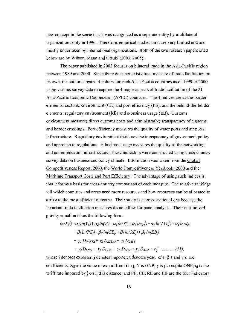
mostly undertaken by international organizations. Both of the two research papers cited

below are by Wilson, Mann and Otsuki (2003,2005).

The paper published in 2003 focuses on bilateral trade in the Asia-Pacific region

between 1989 and 2000. Since there does not exist direct measure of trade facilitation on

its own, the authors created 4 indices for each Asia-Pacific countries as of 1999 or 2000

using various survey data to capture the 4 major aspects of trade facilitation of the 21

Asia-Pacific Economic Cooperation (APEC) countries. The 4 indices are at-the-border

elements: customs environment (CE) and port efficiency (PE), and the behind-the-border

elements: regulatory environment (RE) and e-business usage (EB). Customs

environment measures direct customs costs and administrative transparency of customs

and border crossings. Port efficiency measures the quality of water ports and air ports

infrastructure. Regulatory environment measures the transparency of government policy

and approach to regulations. E-business usage measures the quality of the networking

and communication infrastructure. These indicators were constructed using cross-country

survey data on business and policy climate. Information was taken from the Global

Competitiveness Report, 2000, the World Competitiveness Yearbook, 2000 and the

Maritime Transport Costs and Port Efficiency. The advantage of using such indices is

that it forms a basis for cross-country comparison of each measure. The relative rankings

tell which countries and areas need more resources and how resources can be allocated to

arrive to the most efficient outcome. Their study is a cross-sectional one because the

invariant trade facilitation measures do not allow for panel analysis. Their customized

gravity equation takes the following form:

ln(X;) =al In@$+ a21n(ji1)+ a3ln(Y,')+ a41n(yi')+ a51n(I+ti,')+ a6h(di,)

+PI ln(PEJ +P2 ln(CEJ +P3 ln (EJ ) +P4 ln(EBJ)

+ YI DNAFTA+ YZ DASEAN+ Y3 DLAIA

+ Y ~ D E N G + Y ~ D C H N + Y ~ D S P N + Y ~ D A D J + ~ ~ ......... (I I ) ,

where i denotes exporter, j denotes importer, t denotes year, a 's , p's and y's are

coefficients, Xi, is the value of export from i to j, Y is GNP, y is per capita GNP, tij is the

tariff rate imposed by j on i, d is distance, and PE, CE, RE and EB are the four indicators

introduced above. Several dummy variables are also included for the recipients. DNAFTA,

DAsEAN and DLAIA are 3 dummy variables for trade preferences. DENG, DCHN and DspN are

3 dummy variables for the English, Chinese and Spanish languages respectively. DAD, is

the adjacency dummy. Finally, e is the disturbance term defined to be: eijt =EX+Y~+E,',

where Ex is the fixed effect for exporter, Yr is the fixed effect for time and &,,',is assumed

to follow a normal distribution with zero mean.

The coefficients p's measure how elastic trade from i to j is with respect to each

trade facilitation indicator. Their results are consistent with the expected results. PE, CE

and EB are all significant and positive, while RE is significant in a negative manner.

Based on the magnitudes of the P's, a 1% increase in the port efficiency index would give

rise to the largest improvement in trade than the improvement from the same increase in

other indices. Relaxing regulations gives the second largest improvement, followed by

increasing E-business usage and then lastly by improving customs environment.

However, one problem with the indicators is that they are time-invariant in the model.

Their values reflect 1999 or 2000 trade facilitation status, but one would expect

advancement in the course of the 11 years under study. Additionally, as the authors

pointed out, it is not adequate to just look at the increase in trade flow because there are

costs associated with the implementation of trade facilitation procedures. Improving

facilities at ports can be very costly, while making changes to customs procedures may be

more affordable. Therefore, it may be harder to create an increase in the port efficiency

index, but the opposite may be true for the customs environment index. Moreover, it is

important to include any i'ndirect gains as well because an improved trade environment in

one country benefits all the countries that trade with this country. To conclude, the cost-

and-benefit approach should be employed to design a trade facilitation strategy that is the

most efficient; that is, one that will create the largest net gain. Nevertheless, this model

provides some insights about what the benefits could be and allows for comparisons

between trade facilitation measures and other trade policy measures such as tariffs. It is

postulated that a country can unilaterally improve its trade capacity to mitigate the effect

of tariffs imposed by other countries, which can potentially be hard to eliminate without

engaging in costly lobbying.

The second research paper on trade facilitation in 2005 by these same authors

used the same framework to extend their analysis to global trade between 75 countries.

Since more countries are involved, there are more limitations to acquiring the necessary

data. They relied on a smaller set of survey data to create their trade facilitation

indicators and only analyzed 2000 and 2001 trade flows. Another major difference from

the previous study is the authors looked into both importers' and exporters' indices; that

is, in this more recent paper, exporter's port efficiency, regulatory environment and

service sector infrastructure (formerly termed as e-business usage) indices are also

included in the gravity equation, while the exporter fixed effect is eliminated. More trade

preferential arrangements and language dummies are included as the focus moved from

APEC countries to countries worldwide.

Their results for the indicators all have the expected signs and are generally

significant. Trade flow is the most elastic with respect to the service sector infrastructure

indicator; a 1% increase in this index of the exporter is associated with a 2% increase in

its export. This could be a very good news because this area is perhaps the least

complicated to improve in the sense that it does not require government intervention or

change in legislation. They also found that exporters' indices play a more important

role (that is more significant economically) than importers' indices. They explained that

this is related to having more developing countries (South) than developed countries

(North) in their set, and that the pattern of trade is mainly South-to-North. To further their

analysis on this point, they performed separate regressions for South-to-North trade

(exports from South to North) and South-to-South trade (exports between South

countries). In the South-to-North case, the only importers' indicator that is significant at

the 5% level is the service sector infrastructure indicator. The tariffs imposed on the

exporting countries are not significant. That means tariff is not a significant barrier to

trade in the South-to-North direction. Last but not least, the importance of exporters'

indicators generally increased compared to the pooled regression. However, the story is

quite different for the South-to-South trade, where tariffs can effectively deter exports

from other developing countries, and the regulatory environment of the importing

countries can also significantly change the pattern of trade. One thing in common with

the South-to-North trade is that the influences of exporters' indices are still strong than

importers' indices.

Another innovation of this 2005 paper is the inclusion of the interaction effects

between the port efficiency indicators and countries' geographical characteristics, such as

being adjacent, landlocked, or an island. This inclusion is motivated by the difference in

their accessibility. One problem with their approach is that they did not have a strong

theory on what the expected results should be for the various interaction terms, so their

results may be contrary to general believes and hard to interpret. Nonetheless, the

interaction effects are something that is worth thinking about in future research.

3. Data and Exploratory Analysis

The innovation of this paper is the use of the Trade Capacity Building - Trade

Facilitation data set. This survey-based data set is available at the WTOIOECD Trade

Capacity Building Database Category 33 12 1. This is a very new database, which has

been maintained since November 2002. This database is constructed based on the trade

facilitation definition given earlier in the introductory section. That is, any

"simplification and harmonization of international trade procedures related to the

movement of goods across borders" can be classified as a trade facilitating activity. This

database contains all commitments to trade facilitation from both bilateral and

multilateral sources to recipients between 2001 and 2003 and partial commitments in

2004. Some donors have not completely reported their 2004 trade facilitation projects to

the OECDIWTO as of October 2005. Bilateral donors include Australia, Austria, Canada,

Finland, France, Germany, Italy, Japan, Korea, the Netherlands, New Zealand, Norway,

Sweden, Switzerland, the United Kingdom (UK) and the United States (US). The major

multilateral donors include the European Commission (EC), Asian Development Bank

(AsDB), International Development Association (IDA), International Monetary Fund

(IMF), World Trade Organization (WTO) and World Customs Organization (WCO).

There are 168 recipients; most recipients are underdeveloped or developing countries.

Each record has the following fields: reporter name, donor name, implementing

country, recipient name, year of commitment, start date and end date of the project, value

of commitment in US dollars (USD) in thousands, type of flow, project title and project

description. Reporter is the country or organization reporting the project. Donor name is

the provider of the fund of the project. Implementing country is the country that actually

provides physical assistance or hosts the trade facilitation activity. This field is

particularly relevant when the donor is a multilateral agency or finances its own trade

facilitation project; that is, the donor is also the recipient. Recipient name is the country

benefitting from the project. Some of the funds have not been allocated to any particular

country; these will show up in this recipient field as unallocated or unspecified. Year of

commitment refers to the year in which funds were allocated. Start date and end date tell

the duration of the project. Value of commitment in USD is how much money is put into

the trade facilitation project. Type of flows tells how a project is funded. There are three

types of flows: grants, loans and self-financed. Based on the project titles and project

descriptions, some projects have multiple recipients. This is particularly true for

seminars and training sessions.

In total there are 1644 records, 730 records are financed through grant by bilateral

donors; 688 records are financed through grant by multilateral donors; 56 records are

loan and self-financed projects. The remaining 170 records have not been allocated to

any particular recipients. Of all the trade facilitation commitments allocated to a known

recipient from 2001 to 2004 (720.1 million USD), 54.5% came from multilateral donors

(393.1 million USD). Table 1 and Figure 1 in the Appendix show these results. The

commitments to trade facilitation increased significantly during the four-year period.

There was a close to 200% (from 104 million USD to 309 million USD) increase in

international commitments between 2001 and 2003. This trend continues to year 2004;

with only partial data available as of October 2005, total commitments to trade

facilitation in 2004 sum to 343 million USD, which is over the total in 2003. Table 2 and

Figure 2 illustrate these results. The next two tables, Table 3 and Table 4 break down

trade facilitation commitments by income group and region. These classifications into

income and region are the OECD/WTO classifications. This breakdown is partly

interesting because one would expect the less wealthy parts of the world to receive more

assistance. However, this does not seem to be the case; the lower middle income

countries (LMICs) and the Central and Eastern European Countries and the Newly

Independent States of the Former Soviet Union (CEECNS) received the majority of the

funding. Table 3 computes the average value of project for each income group. The

average value is close to 1 million USD in the CEECNIS, while it is only 0.37 million

USD in the LDCs. On average, a country belonging to the CEEC/NIS income group

receives 11.6 million USD in trade facilitation, while a country in the LDCs classification

only gets allocated 2.4 million USD. Figure 3 shows the trends in different regions. It

seems that the LDCs and LICs began to catch up with the other income groups starting

2003. Table 4 computes similar figures for regions. Europe stands out as having the

highest average value of projects of approximately 2 million USD per project, as well as

having the highest average trade facilitation commitments per country (24 million USD).

North Africa, which has four LMICs and one high income country (HIC), is ranked

second in both categories. Thus, both results suggest that trade facilitation procedures are

not necessarily focused on the LDCs and LICs. However, it is hard to judge whether it is

equitable to provide more funds to the LMICs than the LDCs and LICs because the LDCs

and LICs may enjoy a higher marginal benefit than the LMICs for the same amount of

funding. This may be analogous to the Solow Growth Model, which says growth during

a period when the economy is not very developed is faster than during a period when the

economy is well-developed. As a country is already engaging at a high level of'trade,

relatively more trade facilitation effort must be made in order to create more trade. On

the contrary, relatively less effort may be needed to motivate more trade for countries that

were not trading a lot previously.

Table 5 and Figure 4 show the distribution of funds in each year. Each year most

recipients received 5000 USD to 20000 USD of trade facilitation funding. That means

most of the trade facilitation projects were small in scale. There seemed to be more

large-scale projects in 2003 and 2004 than in 2001 and 2002; the number of recipients

receiving above 5 million USD in 2003 and 2004 more than doubled that in 2001 and

2002. Going from 2001 to 2002, there was a large increase in the number of recipients;

the number of beneficiary countries jumped from 88 to 157. This reflects the increasing

importance of trade facilitation. Having only partial 2004 data is likely to be the reason

for the drop in the number of recipients in 2004.

On the donor side, it is interesting to look at whether donors have regional focus

when making trade facilitation commitments. It is not unreasonable to expect a bilateral

donor to focus on helping countries that are geographically close because trade

facilitation procedures are assumed to benefit donors indirectly as well, and such benefits

may be more readily realized if there is less distance barrier. On the other hand, for

multilateral donors, their objectives may be different from that of bilateral donors.

Multilateral organizations may have a more thorough understanding of "which country is

lacking what", and thus can prioritize and balance these needs more efficiently. Table 6

and Figure 5 show which regions received assistance from a few major bilateral donors,

namely Australia, Japan, France, Canada and the US. Canada, Japan and Australia seem

to agree with the above hypothesis on regional concentration. More than half of

Canada's commitments went to South America. Asia as a whole consumed more than

80% of Japan's commitments. Australia only assisted three regions - Far East Asia,

North and Central America and Oceania. Note also that over 80% of Oceania funding

came from Australia. The US being the largest bilateral donor had quite a diverse

portfolio, except it did not make commitments to Oceania. For the main multilateral

donors on the other hand, the EC and WCO behaved like bilateral donors. Table 7 and

Figure 6 illustrate how the main multilateral donors allocated their funds. It is not

surprising that 70% of EC's resources (3 10 million USD) went to European countries and

CEECINIS; this can explain the results seen in Table 3 and Table 4. However, the focus

on South Saharan African countries by the WCO is phenomenal. This regional focus of

the WCO suggests that customs environment may have significantly improved in South

Saharan African countries. The WTO had a diverse portfolio like the US; however, more

weights (approximately 40%) are put on South Saharan African countries.

After a brief examination of the trade facilitation data, I now return to my

research question: Is trade facilitation the right direction to go in building trade capacity?

Would trade volume between each pair of donor and recipient - in particular exports from

recipient to donor - increase with trade facilitation commitments? This data set on trade

facilitation maintained by the OECDIWTO fits my topic perfectly because it identifies

donor, recipient and value commitment to trade facilitation. The amounts committed to

trade facilitation can be viewed as improvements in trading environment. In WMO 2003

and 2005, they used trade facilitation indices to estimate the effect of trade facilitation on

trade flows. The weakness of their methodology is that there were no variations in their

trade facilitation indices over time. Any change in trade flows between a particular pair

of countries cannot be attributed to different levels of trade facilitation indices because

these indices are the same over time in their framework. Unlike WMO, this paper

utilizes the panel feature of the trade facilitation data set to generate variation in trade

facilitation level. For each donor-recipient pair, I construct for each year how many

funds were provided from this donor to this recipient (TF Bi D-to-R), how many funds

were provided from other bilateral donors to this recipient (TF Other Bi), how many

funds were provided from various multilateral donors - EC, the United Nations, WCO,

WTO and others, and how many commitments were made through loans or self-financed.

A positive commitment would be interpreted as an improvement in trade facilitation.

To use the gravity model, data on bilateral trade flows, GDP, per capita GDP,

tariff rates and distance are needed from 2000 to 2004. The data on bilateral trade flows

are gathered from the United Nations Statistics Division - Commodity and Trade

Database (COMTRADE), volumes are in million nominal USD. Data on GDP and per

capita GDP come from the International Monetary Fund (IMF). The IMF database has

nominal, real and purchasing-power-parity adjusted GDP (PPP GDP) and per capita GDP.

Real values refer to 1990 USD. GDP deflator and purchasing-power-parity US dollar

exchange rate are also available from the IMF database. The use of real GDP and PPP

GDP eliminates the effect of inflation on trade volume and takes into account differences

in general price level in different countries. Tariff rates are from the World Bank

division of the United Nations Conference on Trade and Development (UNCTAD) under

the World Development Indicator category. Tariff rates for 2004 are not available yet. It

will be assumed that there was no change in tariff rates between 2003 and 2004. Tariff

rates for some years were also missing for some countries; the tariff rates for the missing

years will be assumed to be the same as in the previous year. For some countries, tariff

rates were completely missing for all years. In this case, the regional average tariff will

be used. For instance, if country A exports to country B, but the tariff rate imposed on A

by B is not known; if country A is in region C, the tariff rate imposed on country A will

be taken to be the average tariff rate imposed on all other countries in region C. Distance

between each donor-recipient pair calculated using the "great circle distance between capital

cities" method come from two sources http://www.macalester.edu~research/economics/~a~e/

haveman/trade.Resources/Data/ Gravitv/dist.txt and www.indo.com/distance. Besides the

above variables, trading blocs or trade preferential arrangements and language are often

put into the gravity model as well; therefore, I will also investigate the most commonly

included trading blocs and languages. The Asia-Pacific Economic Cooperation (APEC),

Latin American Integration Association (LAIA), League of Arab States (LAS) and

European Union (EU) will be considered. The Central Intelligence Agency (CIA) World

FactBook provides the list of members of each of these groups at http://www.cia.~ov/cia/

publications/factbook/index.html. From the same source, which country uses English,

French, Spanish and Arabic as their primary language can also be identified .

Due to data unavailability and some recipients did not receive funding from

bilateral donors, the number of recipients included in the study is 128 and the number of

bilateral donors included in the study is 14. In total there are 257 donor-recipient pairs in

the analysis. Provided each pair has data for 5 years, from 2000 to 2004, there are 1285

records in total. Details on how the trade facilitation commitments and all other variable

are incorporated into the regression framework are provided in the next sections on

empirical strategies and empirical results.

4. Empirical Strategies

My specification of the gravity model to study the effect of trade facilitation on

bilateral trade is built on Linnemann's model (1966) (Equation 7c):

xij = yo my' ( ~ i ) ~ ~ (E;)y3 (YIY'~ (d0P5 UiJ

However, the trade barrier function - Equation (9) - would not only depend on distance,

but also on tariff and the trade facilitation supports provided by the trading partner and

other bilateral and multilateral sources. If, for two trading partners i and j, country j is a

donor country and country i is a recipient country of trade facilitation commitments, then

Equation (9) becomes:

Tij = Gij(d,j, ti, , TF$,j, TF$B,, TF$M,)

= a0 (dG)"O(l + t ~ "'(TF$~)"~(TF$B~)~~(TF$M~)~~ ... . .. . . . (1 2).

Contrary to distance and tariff, which is positively related to the trade barrier function,

trade facilitation commitments - TF$,, , TF$Bl and TF$M, - should be negatively related

to the trade barrier function because the purpose of these commitments is to facilitate

trade, which can be thought of as to reduce trade barrier. Thus, coefficients a3 to a5

should be negative. This modification (12) gives rise to the following "gravity-type"

equation used in this paper:

xi,'= a ~ ~ ~ ' , a ' ~ ' , a 2 ( y ~ ) a 3 ( y ~ ) a 4 ( ~ ~ $ ~ ) p ' ( ~ ~ $ ~ ~ ) p 2 ( ~ ~ $ ~ ~ p 3 ( d ~ 8 1 ( l + t i ) ' (1 3a),

or in logarithmic form:

ln(X,;) =aoot+al 1n(Y,')+a2 ln(~, ')+ a3 ln(y:)+a;l ln(y,')

+PI ln(~F$:) + P2 In(TF$B;) + P3 ln(TF$M,')

+ Sl ln(di,) + S2 ln(l+t,')+ln(u,') ... ... ... ... ... ... ... (1 3b).

where t denotes year, the constant term is allowed to vary for different years to capture

aggregate economic shock for a given year; that is, time is treated as a fixed effect; Xi, is

the value of the flow from country i (recipient) to country j (donor); Yi (Y,) is the GDP in

i ('j), y, (yj) is the per capita GDP in i 0); TF$,, TF$Bi and TF$Mi are the trade facilitation

commitments received by i from j, the trade facilitation commitments to i from other

bilateral sources and the trade facilitation commitments to i from multilateral sources,

respectively; dij is the distance between i and j; tij is the ad valorem tariff imposed by j on

i's exports; ui,, the disturbance term, is assumed to be log-normally distributed (In u,,' - N(0, 0,)). This equation estimates the behaviour of i's (recipient) exports to j (donor).

Changing Xij to X,i (i's imports from j) and t, to t,, (ad valorem tariff imposed by i on

imports from j) of Equation (13) gives the behaviour of i's imports from j. However, this

direction of flows would not be considered in this paper because the concern is on the

exports of the recipient countries.

The focus of this study is on the P coefficients, which try to estimate the effect of

trade facilitation commitments on trade flows. It is postulated that the p's should be

positive because the introduction or reform of trade facilitation procedures is to enhance

trade. This also follows directly from the fact that trade facilitation commitments are

inversely related to the trade barrier function and the trade barrier function is also

inversely related to trade flows. The other variables in Equation (13) capture other

influences on trade flows. By Anderson's derivation of the gravity equation, the GDP

terms represent the demand and supply of tradeables. The larger the GDP of the exporter

is, the larger the supply of tradeable goods. This is intuitive because a large economy is

associated with high production capability, which in turns increases export capability.

The larger the GDP of the importing country is, the larger the demand for tradeable good.

Therefore, the level of trade should be increasing in both GDPs; that means both a, and

a2 are expected to have a positive sign. For the per capita GDP terms, they are often

used as indicator of the level of development of the two economies. Some researchers

use per capita GDPs as a proxy for productivity (Anderson and Van Wincoop 2003).

When a country is more developed, it becomes more specialized and thus more

productive. This links highly specialized and high per capita income together. With

higher production of fewer goods, such country would need to purchase from foreign

countries items that it does not produce enough for domestic consumption. Therefore,

per capita GDP should be positively related to trade flows (Frankel and Wei 1995 and

Cyrus 2002). This suggests both a3 and a4 are anticipated to have a positive sign. For

the distance (dij) and tariff (t,j) variables, their coefficients 6, and 62 should

unambiguously be negative because they impede trade by creating more costs. This

completes the augmentation of the basic gravity model with the trade facilitation

commitments.

In today's literature, most uses of the gravity model would also include dummy

variables for trade preferential arrangements and primary language variables. These

variables acknowledge the qualitative aspects of trading partners. In earlier empirical

works, researchers either only included trading blocs or tariff rates to capture trade

preferences. However, there exists studies that show both tariffs and trading blocs are

significantly related to bilateral trade flows (Oguledo and MacPhee 1994). Since trade

preferential arrangements may be correlated with tariff rates, they must both be taken into

account in the estimation to create unbiased results. For the language spoken variables,

they can be related to trade volume because communication is an important aspect for

trade to take place. Intuitively, if a country operates using a language that is universally

recognized such as English, then there will be less of a barrier to trade. Language

variables can also be used as proxies for culture background and colonial ties. For

instance, French is the official language of the African countries that were once the

French colonies. With these extensions, the new specification of my gravity model in

logarithmic form is:

In(&]') =aoot+al In(~,')+a~ln(Y,')+ a3 In(y,')+alIn(y,')

+PI ln(TF$,') + P2 ~(TF$B,') + PJ In(TF$Mi[)

+ Y I DAPEC+ ~2 DLAIA+ ~3 DLAS + ~5 DEU

+ Y6 D~n~llsh + Y7 D~rench + Y8 Dspanlsh + Y9 DArabrc

..................... +al ln(d,) + 62 ln(1 +t,[l+ln(u,') (1 4).

This equation pools data for four years since 200 1, the year when trade facilitation

efforts were first made, to do a cross-sectional estimation. The resulting estimations

would tell how each variable is correlated with bilateral trade flow between a donor and a

recipient of trade facilitation commitments. Focus will be put on the exports from the

recipient to the donor because one of the broader goals of facilitating trade is to help the

recipients to climb up the income ladder by expanding their trade capacity. If recipients

can sell their products abroad more after the improvement in trade facilitation, we are one

step closer to this goal.

Usually a cross-sectional analysis can provide insights about association between

variables. It is possible that the association is capturing the natural trends of the

dependent and the independent variables. This motivates the use of the first-differenced

estimation method, which helps to detrend the data. This methodology requires data for

more than one period because it looks at changes. In the trade facilitation context, the

first-differenced estimator would test whether changes in bilateral trade flows can be

explained by changes or additions in trade facilitation commitments. Taking the

difference of Equation (14) for two different periods, t and t-1, would give the first-

differenced equation:

4k+KJ) = A ~ o o + ~ I A ln(I;)+a~ A WI;)+ a 3 A l l n ( y 3 + a ~ A l

+PI A, ln(TF$,)+ P2 A, ln(TF$B,) + P3 A, ln(TF$M,)

.................... +&Al ln(1 +t,S+ A, ln(u,) (15),

where A, is the change between period t-1 and t, for t=2001,2002,2003,2004. Note that

the time invariant terms such as trading blocs, languages and distance drop out of the

first-differenced equation. This equation allows for fluctuations in year-to-year

macroeconomic shocks, national output, per capita income and trade facilitation

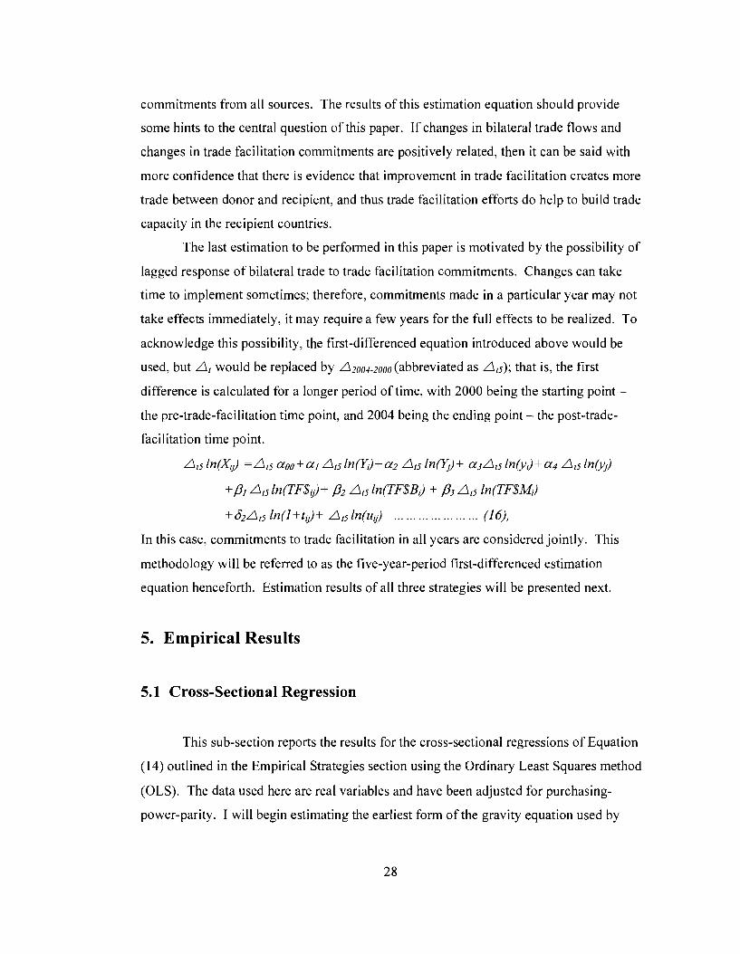
commitments from all sources. The results of this estimation equation should provide

some hints to the central question of this paper. If changes in bilateral trade flows and

changes in trade facilitation commitments are positively related, then it can be said with

more confidence that there is evidence that improvement in trade facilitation creates more

trade between donor and recipient, and thus trade facilitation efforts do help to build trade

capacity in the recipient countries.

The last estimation to be performed in this paper is motivated by the possibility of

lagged response of bilateral trade to trade facilitation commitments. Changes can take

time to implement sometimes; therefore, commitments made in a particular year may not

take effects immediately, it may require a few years for the full effects to be realized. To

acknowledge this possibility, the first-differenced equation introduced above would be

used, but A, would be replaced by A200r-rooo (abbreviated as &); that is, the first

difference is calculated for a longer period of time, with 2000 being the starting point -

the pre-trade-facilitation time point, and 2004 being the ending point - the post-trade-

facilitation time point.

At51n(Xj) = A 5 a00+alA,51n(K)+az A t 5 a3&ln(yJ+a4 Atsln(y/)

+PI A t 5 ln(TF$,/)+ PZ At, ln(TF$BJ + P3 A,, ln(TF$MJ

+&At5 ln(l+t,i)+ A,ln(u,j) ... ... ... ... ... ... ... (16),

In this case, commitments to trade facilitation in all years are considered jointly. This

methodology will be referred to as the five-year-period first-differenced estimation

equation henceforth. Estimation results of all three strategies will be presented next.

5. Empirical Results

5.1 Cross-Sectional Regression

This sub-section reports the results for the cross-sectional regressions of Equation

(14) outlined in the Empirical Strategies section using the Ordinary Least Squares method

(OLS). The data used here are real variables and have been adjusted for purchasing-

power-parity. I will begin estimating the earliest form of the gravity equation used by

Tinbergen, to check if my data set can produce similar results. That is, the first

estimation will only use national income and distance as regressors. Then, the basic

model will be augmented by including the per capita income, tariff, trading blocs and

languages. Table 8 shows the results of each of these estimations. The last set of

estimations in this sub-section is the key estimation and it is shown in Table 9; it will

include all the trade facilitation variables into the gravity model.

The second column of Table 8 confirms that the gravity model fits my bilateral

trade data set well; the portion of variation in bilateral trade that can be explained by

income and distance is 67%. Economic conditions in 2004 seemed to be significantly

better than 2000. Exports from recipients to donors were 65% (exp(0.507)= 1.65) more in

2004 compared to 2000. Similar to other trade studies, there is evidence that higher

incomes are associated with higher level of trade, and distance also significantly reduces

trade volume. Recipient's exports are found to be elastic with respect to the recipient's

GDP; this result is also consistent with other studies. This exercise is mainly used as a

check for the suitability of applying the gravity model to my particular sample of trading

partners (donor-recipient pairs). The results support such application.

The fourth column of Table 8 shows the most commonly used gravity model in

the literature. It incorporates the per capita income, tariff, trade preferential arrangements

and language variables. The adjusted R~ remains high at 0.73, meaning that these newly

added variables are useful. Income and distance are still significant with the expected

signs. The income level of the recipient has a positive and statistically significant effect

on trade; a 10% increase in recipient's per capita GDP is associated with a 3% increase in

its exports. However, the donors' per capita GDP does not have much impact on how

much the recipients export to them. This could be explained by the fact that all these

donors are wealthy developed countries, the variation in income level is trivial. Tariff on

recipients' exports affects trade negatively but not in a significant manner. This

corresponds to what WMO reported in their 2005 trade facilitation paper, where they

found that South-to-North trade is not significantly affected by tariff. Next, recipient

countries that use English or Spanish tend to trade significantly more, but recipient

countries that use French or Arabic tend to trade significantly less, than countries that use

other languages. This also agrees with WMO findings. Lastly, for the trading blocs,

countries belonging to the Asia-Pacific Economic Cooperation (APEC) and League of

Arab States (LAS) groups trade significantly (about 3.7 times) more than countries not

belonging to these groups. The result for APEC may be explained by the rapid growth in

the Asian economy, but the reason for the LAS result is less clear.

The first set of estimations in Table 9a shows the effects of the nine trade

facilitation commitment variables. The donor-to-recipient commitment (TF Bi D-to-R) is

marginally insignificant at the 5% level. A 10% increase in the trade facilitation

commitment from a donor to a recipient would increase exports from this recipient to this

donor by 0.2%. For other bilateral sources (TF Other Bi), the effect on the trade between

any given pair of trading partner is significant. A 10% increase in other bilateral trade

facilitation commitments would increase trade by 0.3%. For the multilateral

commitments, sources are divided into the European Commission (TF EC), United

Nations Development Account (TF UN), World Customs Organization (TF WCO) and

World Trade Organization (TF WTO) and other multilateral sources (TF Other Multi).

This classification is based upon two criteria. First is their importance in terms of amount

of commitments and second is their relevance to trade issues. The EC and UN satisfy the

first criterion, and the WCO and WTO satisfy the second. It shows that multilateral

sources are related negatively to exports from recipients to donors, and these negative

relationships are significant except for WCO. This might be a good example of a

regression showing association rather than effect. It seems more reasonable to interpret

the negative signs for the multilateral commitments as "more multilateral commitments

are spent on relatively low-trade-exposure countries" than as "the more multilateral

commitments are made, the less trade there will be from recipients to donors". The

different results found for the two types of donors may not be as surprising as it seems

because the goals of multilateral agencies may be different from the goals of bilateral

donors, with the former trying to promote equity around the world and the lateral

focusing more on their own national interests. Lastly, the loan and the self-financed

commitments are both insignificant. The adjusted R~ for this model is 0.74, and the

estimates of the other variables are robust to the addition of the trade facilitation variables.

Note that, this regression is run for year 2001 to 2004 because trade facilitation

commitments only started in 2001.

Column five of Table 9a aggregates all the bilateral trade facilitation

commitments into a single variable to show the total bilateral effect (TF All Bi). This

new variable has a positive and significant effect on trade. The estimate shows that a

10% increase in bilateral commitments as a whole is associated with a 0.4% increase in

recipient-to-donor trade. The estimates of the other variables virtually do not change

under this modification. Table 9b is a continuation of Table 9a. The first set of

regression in Table 9b is a duplication of column two and three of Table 9a for

comparison purposes. Column four of Table 9b aggregates all the bilateral trade

facilitation commitments into a single variable (TF All Bi) and all the multilateral trade

facilitation commitments into another variable (TF All Multi). The results say that a 10%

increase in the overall level of bilateral commitments is associated with a 0.4% increase

in bilateral trade, and a 10% higher in the overall level of multilateral commitments are

related to a trade volume that is 0.6% lower. Both results are statistically significant.

Column six further aggregates the bilateral and multilateral commitments into one entity

(All TF). However, the positive effect of the bilateral commitments and the negative

effect of the multilateral commitments seem to have cancelled each other out that the net

effect is insignificant. Again with these modifications, the estimates for the other

variables remain quite stable. Although it is hard to establish causal relationship here, it

is clear that trade facilitation commitments are related to trade in some way. This

corresponds to what WMO found when they used trade facilitation indices to measure the

level of trade facilitation across countries. Based on the above results, it appears that

combining all the bilateral commitments into one variable is plausible because there does

not seem to have much gain in distinguishing between the two. On the other hand, it may

be better and useful to keep each multilateral source of commitments separately because

of their very different nature and scope. This scheme of using a single bilateral

commitments variable and several multilateral commitments variables will be used in the

next part - the first-differenced estimation.

Often in doing cross-sectional regressions, one may worry about the error terms

not being homoskedastic. Two proposals are suggested here to address this concern.

First is to use the White hetero-robust standard errors instead of the OLS standard errors.

These are shown next to the OLS standard errors (column 4 and 7) in Table 9a. The

significance of the trade facilitation variables, as shown by the asterisks beside the robust

standard errors estimates, does not change significantly. This implies that the above

results are robust. The second proposal is to use the weighted least squares (WLS)

method, which is commonly used in econometric studies to handle heteroskedastic data.

The weights to be used here are the population size of the recipient countries (Frankel

and Wei 1993). Variance of errors is assumed to vary inversely with population size;

therefore, more weights would be given to countries with a larger population. Results for

this WLS estimation are shown in Table 10. In general, the results are similar to that in

Table 9a. The coefficient of the bilateral commitments (TF Bi D-to-R) drops from 0.021

to 0.014, while that of the other bilateral commitments (TF Other Bi) rises from 0.03 1 to

0.036; both terms become more statistically significant in the WLS estimation. For the

aggregate bilateral commitments (TF All Bi), there is a drop from 0.040 to 0.032. In both

bilateral commitments specifications, the UN commitments become insignificant. WCO

commitment is still insignificant but in the WLS regression, it takes a positive value.

While loan remains insignificant, self-financed trade facilitation commitments become

significantly negative. This suggests that countries that have not been engaging in much

trade tend to finance trade facilitation projects themselves. As mentioned before the

donor and recipient of a self-financed project are the same country. Some developing

countries may see the need to engage in trade facilitating activities; however, due to lack

of expertise perhaps, they must acquire expertise from developed countries or multilateral

agencies to implement the trade facilitation projects for them.

In reviewing the gravity models used by other researchers, different units of

account were used. Some used nominal values (Bergstrand 1985), some used real values

(WMO 2003, 2005) and some used nominal values but also include price indices

(Thursby and Thursby 1987). In table 11, I re-estimated Equation (14) using nominal

values, real values based on 1990 USD and nominal values adjusted for purchasing-

power-parity (PPP), standard errors shown are the hetero-robust standard errors. These

three estimations are to be compared to the first set of estimates in Table 9a. These

estimates vary somewhat from the estimates using real PPP values. In particular, the

bilateral and the WTO commitments become insignificant in all cases. The magnitude of

other variables also changes by a considerable amount. It seems like the real values

estimates depart from the real PPP estimates by the most, followed then by the nominal

values. The nominal PPP values seem to give the closest results to the estimates using

the real PPP values. This suggests that the metric choice may change one's results, so

one must be aware of such possibility. Ideally, the real PPP values should be used

because it eliminates the effect of inflation and incorporates the differences in price level

across nations. Therefore, the remaining analyses will be performed on the real PPP

values.

5.2 First-Differenced Estimations

As mentioned before, trends may obscure the cross-sectional estimates, this

section attempts to remedy this drawback of the cross-sectional estimations. Equation

(1 5) in the Empirical Strategies section is the equation to be estimated here. The first

difference is calculated based on annual data. Since there are four years of trade

facilitation commitments, there are in total four differences for each donor-recipient pair

if data are available. The estimation results are provided in Table 12. The second

column was obtained using OLS, the fourth column gives the White hetero-robust

standard errors and the fifth column shows the WLS estimation. Before going through

each of the trade facilitation variables in detail, it is noted that the robust standard error

are very close to the standard error produced by OLS. However, due to the differencing,

a large portion of the variation in the variables has been cancelled out. This results in a

small R2 of 0.1 5 for the OLS first-differenced estimation. The WLS method, again using

recipient's populations as the weights, improves the explanatory power of the model by

about 25%. These phenomena on R2 are not unexpected as explained above, thus, this

statistic is only reported for completeness.

From the OLS estimation, most variables do not significantly influence changes in

exports in a statistical sense. For the year-to-year economic fluctuations, only the fixed

effects between year 2003 and 2004 differ by a significant amount. The aggregate shock

experienced in 2004 on top of the aggregate shock experienced in 2003 is positively

affecting trade flows from recipients to donors. This shock in 2004 is estimated to

increase exports from recipients to donors by 1 1 % (exp(O.107)=1.11) from the level of

exports in 2003. Focusing back to the trade facilitation variables, there is evidence that

the investments made by WCO in trade facilitation paid off. A 10% increase in WCO

commitment is related to 0.27% increase in recipients' exports to donors. Although this

number is small numerically, it can quite potentially be translated into large increase in

exports because by looking at Table 7, WCO only made a total of 378,110 USD

commitments to trade facilitation. This amount can easily be doubled, and thus produce a

2.7% increase in exports from recipients to donors. Based on the robust standard error,

the combined commitments of multilateral agencies (TF Other Multi), besides those

explicitly included institutions, also have similar positive effect on trade as WCO

although the evidence is not as strong. All other trade facilitation variables do not seem

to have any effect on exports according to this OLS estimation.

Using the WLS method, so that more weights are given to the larger countries, the

estimates should be more efficient than the OLS estimates. The results obtained with

WLS indeed fit more comfortably with the general belief. A higher increase in the

recipient's per capita income would induce a higher increase in exports. This seems to

agree with the saying that richer countries tend to trade more (Cyrus 2002). Donor's

economic factors do not seem to have much impact on the pattern of change in recipients'

exports. In this estimation, an increase in the tariff rate on recipients' exports has the

expected negative effect. This effect is also a significant one. A 1% increase in tariff

rate will inhibit exports from recipients by 2.72%. Comparing the results for the

"generic" gravity variables in the two estimation methods shows a large degree of

discrepancy. However, for the trade facilitation variables, the two methods give rather

similar results. In particular, the significance found in OLS for the WCO commitments

appears in WLS as well, with a comparable magnitude of 0.023. In WLS, WTO

commitments would marginally (with a p-value of 0.088) decrease exports by a very

small and possibly negligible amount (1% increase in WTO commitment would give rise

to a 0.003% decrease in exports). The commitments from other multilateral sources

would not significantly alter exports pattern in this case, the same is true for bilateral

commitments. As an additional remark, for this first-differenced estimation methodology,

I also checked the different specifications of the bilateral and multilateral commitments

as in Table 9. When bilateral (TF Bi D-to-R) and other bilateral commitments (TF Other

Bi) enter into the equation separately, the same results are observed - particularly the

effect of WCO commitments remains strong. All forms of aggregation between and

within bilateral and multilateral commitments would produce insignificant estimates

because they are likely to cancel out each other's effect.

Now compare the first-differenced results with the cross-sectional regressions

from before. The positive shock in 2004 shows up in both estimations. Among the

multilateral donors, WCO is the only one that is not significantly negatively correlated

with trade in the cross-sectional analyses and it also is the only one that is clearly

positively correlated with trade in the first-differenced analyses. This can be considered

as an informal qualitative cross-check or confirmation procedure. To summarize, the

lesson learned from this first-differenced estimation is that changes in exports from

recipients to donors covariate positively with changes in WCO trade facilitation efforts.

The last equation to be estimated is Equation (16), the five-year-period first-

differenced estimation equation. By allowing for a longer response period - five years,

this may be able to capture the longer term and cumulative effects of trade facilitation

efforts if they exist. Since this equation is merely a slight variation of Equation (1 5) , the

same procedures will be used to perform the estimations - OLS, OLS with hetero-robust

standard errors and WLS with population size of recipient countries as weights. The

estimation results are tabulated in Table 13. The most remarkable result in Table 13

perhaps is the strong impeding effect of tariff on trade over the 5-year period of study,

with a 5.53% decrease in recipients' exports for every 1% increase in tariff against

imports from recipients. The second observation is that the R~ is significantly higher in

the 5-year-period first-differenced estimation. With OLS, the proportion of variation in

changes in exports that can be explained by the variables listed is 0.37; with WLS, this

proportion jumps up to 0.70, which is considered to be quite high for first-differenced

estimations. However, this is by no means a "standard" first-differenced estimation.

With OLS, the changes in exports over a five-year period are related positively to

changes in EC's trade facilitation commitments. This is a weak relationship, and cannot

be stated with a high degree of confidence when WLS estimation is used. However,

trade facilitation commitments financed through loan by the recipients themselves do

show some positive influence on their exports to donors, and this result is robust across

estimation procedures. With WLS, the results for WCO and WTO commitments found

in the one-year-period first-differenced estimations appear in the 5-period difference as

well. The size of the effects gets magnified considerably in the 5-year-period difference.

For WCO, the 1-year-period effect is 0.023 and the 5-year-period effect is 0.04 1. For

WTO, the 1 -year-period effect is -0.003 and the 5-year-period effect is -0.034. From a

brief look at the project description available in the trade facilitation database, WCO

tends to participate in more actual fieldwork, such as visiting and assessing facilities; its

scope is also very wide, its projects involve all four sub-categories of trade facilitation -

customs environment, port efficiency, regulatory environment and service

infrastructures - implemented in various forms. They organize practical training sessions,

workshops and seminars. The robust positive effects on trade attributable to WCO

commitments may be a result of their ability to deliver the suitable form of assistance to

the beneficiary countries. WTO, on the other hand, mostly gives seminars and seldom

provides other forms of assistance. This may partly explain the negative relationship

observed. However, there might be many other policies and shocks that took place

during the 5 years, and that their effects might not have been properly controlled for in

the estimation. One must exercise caution when interpreting the results. Lastly, it is

useful to look at how much change in trade is realized after improvement in trade

facilitation. It is found that the total increase in trade would be 361 million USD.

This completes the quantitative analysis section of this paper. The trade

facilitation database used in this paper is very rich in qualitative terms because it contains

project descriptions. These project descriptions provide a channel for a deeper

understanding of this relatively new field of trade facilitation. The next section would

give a more thorough direction on how this data set can be further utilized and what the

other issues are regarding trade facilitation.

6. Future Research

Trade facilitation, being a very young area of research, has a long way to grow.

The OECDIWTO Trade Capacity Building - Trade Facilitation Database provides useful

information for exploration. Not only does this database show how much aid was given

by whom to whom, most of its projects are also accompanied by a description outlining

what type of work has actually been done. One can make use of these descriptions to

classify projects into the four categories of trade facilitation and then estimate how trade

flows respond to improvement in each of these categories. This exercise has strong

policy relevance because negotiations on trade facilitation commitments are likely to

continue in the foreseeable future. It is important that these resources are put into their

best possible use and are distributed equitably.

In this paper, only the increment in trade facilitation and bilateral trade resistance

are considered. Ideally, one would want to control for the multilateral trade resistance

that a country faces as in Anderson and Wincoop (2003) and the trade facilitation status

when evaluating the effects of increment in trade facilitation. When a country is already

operating at a reasonable level of trade facilitation, any additional commitment to trade

facilitation may not create much impact on trade. One the other hand, if the initial level

of trade facilitation is low, a small increment in trade facilitation may lead to enormous

increase in trade. However, finding a good measure of the initial trade facilitation level

may be a difficult task because using survey data like WMO may result in selection bias.

There will be less data or even no data for countries that trade very little, and thus it will

be more difficult to assess the actual level of trade facilitation for these countries.

Another extension of this project can be to look beyond trade between each pair

of donor and recipient of trade facilitation commitments. One can study whether the

exports of a recipient to all of its trading partners or the total exports of a recipient

experienced an increase after the implementation of certain trade facilitating procedures.

The main reason for limiting this paper to the donor-recipient trade is that bilateral donors

are likely to have stronger ties to their choice of recipients than other countries that they

did not assist. Any gain in trade due to increment in trade facilitation should be more

pronounced between donor-recipient pairs, and thus more easily identified.

Another possible stream of research is to assess the results and usefulness of the

previously implemented trade facilitation procedures. Using trade volume as an

instrument to evaluate the effectiveness of these projects is one strategy. Other method to

appraise trade facilitation projects is to review surveys on trade facilitation performance

submitted by recipients, reporting countries or observers. However, these surveys have

not yet been publicized or done extensively; this form of assessment may not be feasible

at this time.

7. Conclusion

This project investigates whether trade facilitation efforts can help the less

developed and the developing countries to engage in more trade. In particular, can trade

facilitation commitments from bilateral and multilateral sources successfully build trade

capacity in these countries such that they can integrate themselves into the world of trade?

The relationship between trade facilitation and trade capacity is connected or linked

through trade volume. If trade originating from a country became more frequent after it

received some aid in trade facilitation, this would be considered as a success in building

trade capacity via trade facilitation activities or programs. By using the OECDIWTO

Trade Capacity Building - Trade Facilitation Database that contains bilateral and

multilateral commitments to promoting trade facilitation in less developed countries

between 2001 and 2004, a few models have been estimated to examine the effects of such

commitments on trade flows. The cross-sectional analyses reveal that bilateral

commitments are significantly positively correlated with exports from a recipient to its

donor. For the multilateral commitments, this relationship is found to be negative. With

the first-differenced estimator, there is evidence that WCO commitments are trade

facilitating. Its effect on trade is estimated at 0.23% to 0.41% increase in recipient-to-

donor trade for every 10% increase in WCO commitments. Finally, this project only

looked at a few aspects of the relationship between trade facilitation and trade. There are

many areas remained to be studied. Undoubtedly, more and more information will

become available in this field, and this will allow for more detailed analyses to be done in

the future.

Appendix A - Detailed Derivation of the Gravity Equation

As introduced in the literature review section, Anderson (1979) was the first one

to provide a theoretical framework for the gravity equation. This annex will show how

Anderson derived the gravity equation using the trade-share-expenditure system model.

Assume that all countries have a traded good sector and a non-traded good sector

and the utility function is a weakly-separable one: u=u(g(traded goods), non-traded

goods), where the function g(traded goods) is Cobb-Douglas in its argument. This

property allows for the maximization of the utility from traded goods to subject to the

budget constraint for traded goods only. This in turn gives j's demand for i's tradeable

good (i exports to j):

Mij = Oi $j YJ ...... (A. I), where

0. = j's total expenditure on i's tradeable good ...... (A.2) j's total expenditure on all tradeable goods

..... j's total expenditure on all tradeable goods = F(Yj, Nj). (A.3). $J = j's total expenditure

Yj is the importing country's national income. By Chenery (1960)' $, can be well-

explained by income (Y) and population (N).

With balanced trade,

YI $i = 0i(C $j Yj) ...... (A.4).

That is, the value of imports of i and domestic tradeable purchases must equal to the

value of exports of i and domestic tradeable sales. Substituting (A.4) into (A.1):

If, as a result of long-term capital account transactions, which is a function of Yi and Ni ,

ml=m(Yi, Ni), the trade balance condition changes, then (A.4) becomes:

Yi 4, mi = 0; ( C $j Yj) ...... (A.6).

Under this circumstance, (AS) can be re-written as:

Since xi CI Mij = ( C 4, YJ) by (A. I), (A.7) can be estimated by:

where Uij is a log-normal disturbance, where E(ln(Uij))=O.

By imposing a log-linear form on both m and $:

ml (Yi, Nl) = km ( ~ i ) " ' ( ~ i ) " ~ . . . . . . (A.9),

$I (Y 1, Nl) = ke ( ~ i ) " . . . . . . (A. 1 O),

and substituting (A.9) and (A. 10) into (A.8), the following is obtained:

Mi, = k' km k t (Y i) m l + @l+lWi)m2+ 42 ( Y , ) ~ ' + ' ( N , ) ~ ~ U,, . . . . . . (A.ll).

This is the same as Equation (5) in the main text.

To realistically estimate trade flows, it is necessary to extent (A. 11) to include

flows of many goods between countries, tariffs and transport costs. The following

derivation illustrates this extension using identical preferences for traded goods across

countries and goods in the same commodity class are differentiated by place of origin.

Tariffs and transport costs increase the landed value of i's good when it arrives at the

importing country (i). Let TiJk be the adjustment factor for i's exports of good k to

country j, and Mijk be the value of flows of k from i to j evaluated at the exporter's port

before shipment. Thus, the landed value at country j of good k from country i equals to

Mijk TIJk . With identical preferences for traded goods, the propensity to good k from

country i, eik(Tj) depends on (zj) which is a vector representing resistance to trade

imposed by j due to either geography or trade policy on different goods from different

origins. This gives a more complicated version of (A. 1):

Mljk Tijk = eik(Tj) $j Yj . . . . . . (A. 12).

Aggregating across commodity to get the aggregate flow M,:

My = xk Mijk = $j Yj ( I k (I /TIJk) eik(Tj)) . . . . . . (A. 13).

With balanced trade,

Yi $1 ml = & Mij = $j Yj (xk (l/~?jk) eik(~j)) . . . . . . (A. 14).

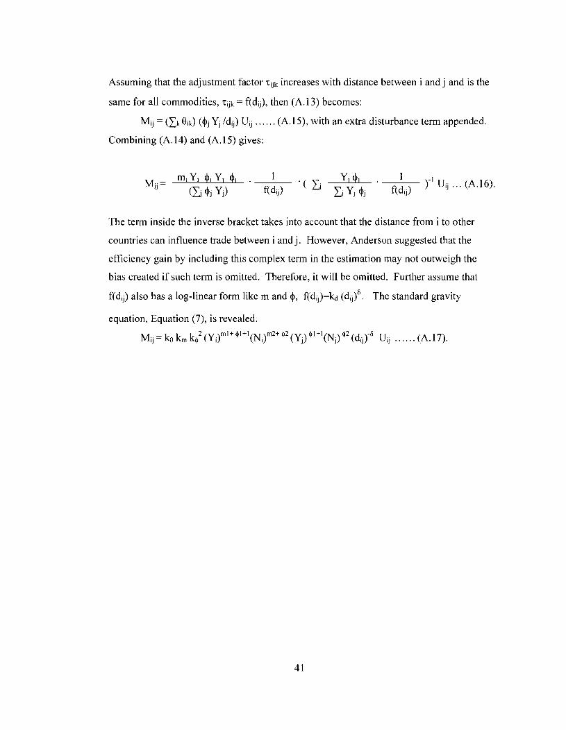
Assuming that the adjustment factor z,;k increases with distance between i and j and is the

same for all commodities, ~,;k = f(d,;), then (A.13) becomes:

Mi; = (x r; eik) (4; Y; Idij) Uij . . . . . . (A. 1 5), with an extra disturbance term appended.

Combining (A. 14) and (A. 15) gives:

M.. = miYi $i Yi $i . 1 Yi 4i . 1 IJ

( C 4; Yj) f(d,j) ' ( XI Y, 4, f(di;) )-I U,; . . . (A. 16).

The term inside the inverse bracket takes into account that the distance from i to other

countries can influence trade between i and j. However, Anderson suggested that the

efficiency gain by including this complex term in the estimation may not outweigh the

bias created if such term is omitted. Therefore, it will be omitted. Further assume that

f(dl;) also has a log-linear form like m and 4, f(di,)=kd (di;)" The standard gravity

equation, Equation (7), is revealed.

M.. = k IJ 0 km k t (~ i ) " ' " ' * ' (N i )~~~ " ( Y ~ ) ""(Nj) 42 (dij)-6 Uij . . . . . . (A. 17).

Appendix B

Table 1. Distribution of Trade Facilitation Commitments by Donor Type (million USD)

Figure 1. Trade Facilitation Commitments from Different DonorType

450.0 , . -- - .-

Donor Type Bilateral Multilateral Loadself-financed Unallocated TOTAL

Bilateral Multilateral Loaniself- financed

Total No. of Records

730 688

2001-2004 92.6

393.1

Table 2. Distribution of Trade Facilitation Commitments by Year (million USD)

Total No. of Records (with nonzero value)

643 629

234.4 172.1 892.2

56 170

1644

Donor Type Bilateral

Figure 2. Trade Facilitation Commitments by Year

3 8 155

1465

Multilateral TOTAL

2001 23.2 81.1

104.3

2002 1 2003

106.2 136.2

2004 54.1 30.0

All 169.2 62.0

246.6 308.6

289.1 343.2

723.0 892.2

Table 3. Distribution of Trade Facilitation Commitments by Income Group and Year (million USD)

Income Group 2001 2002 2003 2004 CEEC/NIS 28.4 22.7 56.3 32.1 LDC 17.9 3.1 51.8 39.2 112.0 LIC 7.3 7.1 26.7 78.2 LMIC 11.0 58. 1 121.9 96.5 287.5

Unallocated 22.4 36.7 1 43.8 1 29.2 TOTAI, 104.3 136.2 1 308.6 1 343.2

I No. of 1 Average value I No. of / Average ~ a q

/ LDC 1 299 / 0.37 1 5 0 I 2.24 I

Income Group CEEC/NIS

LIC LMIC

Figure 3. Trade Facilitation Commitments from Different Donor Type

140.0

Projects I of Project

UMIC Unallocated TOTAL

CEECINIS L DC L IC LMlC UMlC 1

Countries 12 147

216 44 1

each countr 1 1.63 0.95

223 139

1465

5.42 6.39

0.55 0.65 0.46 0.95 0.61

2 2 4 5 53 N/ A 182 4.90

Table 4. Distribution of Trade Facilitation Commitments by Region Group and Year (million USD)

Average Value to each country

12.41 24.02 4.30 0.79 1.94

22.20 0.17 4.68 0.68 2.29

4.90

Region Group CEEC/NIS Europe Far East Asia Middle East North & Central America North Africa Oceania South & Central Asia South America South of Sahara Africa Unallocated America Unallocated Asia Unallocated LDC Unallocated Unallocated TOTAL

No. of Projects

179 97 187 69 150 86 43 172 114 285

9 3 10 4 5 7

1465

Average value of Project

0.97 1.98 0.39 0.16 0.36 1.29 0.07 0.46 0.07 0.39 1.14 0.45 0.77 0.95 0.89 0.61

No. of Countries

14 8 17 14 28 5 18 17 12 49

182

Table 5. Distribution of Funds to Recipients by Year

Total Funding Under 5000 USD 5000-20000 USD 20000-50000 USD

No. of Recipients 2001 / 2002 1 2003 / 2004

50000- 100000 USD 100000-200000 USD 200000-500000 USD

"

go , . . . . . . . . ... . . .. . .. .. ... . . .. ........... " lo Under USE) 5000

4 1 32 1 2 2 2 18

500000- 1500000 USD 1500000-5000000 USD Above 5000000 USD Total

Fiaure 4. Distribution of Funds bv Year 7l

5

7 8 10

2002

Year

54 2 1

6 7 6 8 8

I '13 USD 50000-100000

USD 1000110-200000

10 5 15

0 USD 200000-500000

I IB USD 500000-1500000

78 16

6 8 6

157

2004 Im M o v e USD 5000000

L i

3 9 8

9 6 10

7 7 5

1 1 6 14

152

10 8 12 10 1

Table 6. Region of Trade Facilitation Concentration of Major Bilateral Donors (USD thousand)

- Region Group

CEEC!NIS Europe Far East Asia

Australia 0.0

Middle East North & Central America North Africa

I South of Sahara I 0.0 1 210.3 1 228.8 1 292.5 1 8567.7 1

0.0 3058.6

Oceania South & Central Asia

Japan 23.2

0.0 1402.8

0.0

I

1 Figure 5. Region of Trade Facilitation Concentration of Major Bilateral Donors 1

21.0 1109.2

2680.4 0.0

Canaaa

France 268.8

62.1 8.2 0.0

South America Total

France

Japan

,ustraha

Canada 8.4

57.5 1906.7

157.8 53 1.2

15.2 2138.2

0.0 7141.8

C E E C I Y ~ ' ~ IJ Europe

Far East Asla

Mlddle East I

I

0.0 5248.2 34.0

15.1 86.6 1 12.5

rn Norm 8. Central 1 Amerlca

0 Norm Afrlca I

Oceanla i

7.1

15.5 12333.1 0.0 0.0

243.6 2919.6

0 South S Central Asia

S o u t h of Sahara i

0.0 1.3

627.3 1186.4

0.0 24205.2

1556.4 76168.3

Table 7. Region of Trade Facilitation Concentration of Major Multilateral Donors (USD thousand)

Region Group CEECINIS

I Middle East 2 12.58 / 1.29 1 196.04 1 Europe Far East Asia

EC 125584.90

I Oceania 1 0.00 1 0.00 1 53.80 1

1 85 107.20 14043.74

North & Central America North Africa

WCO 9.66

1 South America 1 94.24 1 3.45 1 146.98 1

WTO 2 17.92

0.46 0.08

2986.10 86513.16

South & Central Asia South of Sahara

Total / 443123.86 1 378.11 1 2082.29 1

87.83 149.83

Figure 6. Region of Trade Facilitation Concentration of Major Multilateral Donors I

4.74 0.00

26702.42 1879.52

nCEEC'NIS 1 ta Europe

I OFarEss tAs ia .

0 Middle East 1 North 8 Central I

129.20 129.20

America I I North Afr~ca ,

12.34 346.09

Y south Central , , AS ia

S o u t h of Sahara

229.97 74 1 .52

Y South America I

Table 8: Cross-Sectional Regression - Standard Gravity Model

Recipient Export Year200 1

Recipient PCGDP Recipient GDP

Coefficient -0.047

Donor PCGDP Donor GDP distance

1.180***

tariff

I LAIA I I 1 0.016 1 0.168 1

SE 0.157

0.873*** -0.983***

French Spanish Arabic

0.025

-2.308

Coefficient -0.082

0.052 0.075

English 1.880

-0.706*** 0.536*** -1.305***

APEC LAS

I No. of Obs. 1 1230 1 1230

SE 0.144

0.307*** 1.074***

0.182 0.155 0.431

EU Constant

0.064 0.029

0.195 0.946*** -0.997***

0.831***

1.306*** 1.327***

0.23 1 0.052 0.080

0.135

0.146 0.435

12.372***

R2 adj. R*

0.697

Significance: 1%: ***, 5%: **, 10%: *

0.669 0.667

0.730 0.726

-0.212 18.182**

0.263 8.987

Table 9a. Cross-Sectional Regression - Trade Facilitation Variables

Recipient Export Year2002

All TF Loan 1 0.000 10.019 10.019 1 0.001 1 0.019 [ 0.019

TF Other Bi TF EC TF Other Multi TF UN TF WCO TF WTO All Bi All Multi

Coefficient 0.1 1 1

0.011 0.012

0.03 1 *** -0.042***

SE 0.168

-0.148* -0.042*** -0.020 -0.037**

Self-Financed 1 -0.039 1 0.025 Recipient PCGDP ] 0.347*** 1 0.072

SE 0.168

Robust SE 0.164

0.011"' 0.011"'

Recipient GDP Donor PCGDP Donor GDP distance

0.084 0.015 0.038 0.017

0.026 0.078"'

Robust SE 0.163

-0.043***

1.060*** 0.346 0.95 1 *** -0.996***

3.019 0.163***

tariff English French 1 -0.706*** Spanish 1 0.403**

Coefficient 0.109

0.059'' 0.015"' 0.037 0.016"

-0.041 1 0.025 0.350*** ] 0.072

Arabic LAIA APEC LAS EU

0.012

0.027 0.078***

0.034 0.269 0.058 0.088

-2.973 0.640***

0.208 0.176

Constant No. of Obs. R~

0.01 I*** -0.142* -0.044*** -0.02 1 -0.038** 0.040***

- 1.460*** -0.045 1.173*** 1.48 1 *** -0.168

I adj. R' 1 0.740

0.038"' 0.281 0.062"' 0.079"'

2.095 0.157

0.270"' 0.132"'

18.553* 983 0.747

1 0.741

0.084 0.015 0.038 0.017 0.013

0.472 0.186 0.165 0.475 0.291

Significance: 1%: ***, 5%: **, 10%: *

0.059** 0.015*** 0.037 0.016** 0.013***

1 .062*** 0.341 0.951 *** -1.010***

-0.697*** 0.398**

10.013

2.088 0.157

3.056 0.162"'

0.541"' 0.130 0.150"' 0.557"' 0.194

0.034 0.269 0.056 0.088

-2.907 0.634***

0.209 0.176

14.846 983 0.747

0 . 0 3 8 ~ 0.280 0.062*** 0.080***

0 . 2 7 0 ~ 0.132***

-1.462*** -0.048 1.170*** 1.453*** -0.229 18.308* 983 0.747

0.472 0.186 0.165 0.475 0.288

0.547*** 0.130 0.150*** 0.563*** 0.190

9.978 14.660 983 0.747

Table 9b. Cross-sectional Regression - Trade Facilitation Variables

I RecipientExport I Coefficient I SE I Coefficient ( SE 1 Coefficient 1 SE ]

TF Bi (D-to-R) TF Other Bi TF EC TF Other Multi TF UN TF WCO TF WTO

I Loan 1 0.000 1 0.019 1 0.004 1 0.019 1 0.006 10.019 1

0.021* 0.03 I*** -0.042*** -0.148*

TF All Bi TF All Multi All TF

Significance: 1%: ***, 5%: **, 10%: *

0.01 1 0.01 1 0.012 0.084

-0.042*** -0.020 -0.037**

0.0 15 0.038 0.017

0.040*** -0.062***

0.013 0.012

-0.006 0.0 14

Table 10. Cross-Sectional Regression - Weighted Least Squares

I WLS WLS Recipient Export Year2002 Year2003

TF Other Bi TF EC TF Other Multi

I Self-Financed 1 -0.093*** 1 0.020 1 -0.096*** 1 0.020 1

Coefficient -0.207** 0.197*

TF UN TF WCO TF WTO TF All Bi Loan

0.036*** -0.030*** -0.164

I Donor PCGDP 1 0.386** 1 0.162 1 0.401** 1 0.163 1

SE 0.084 0.117

-0.006 0.036 -0.042***

-0.002

Recipient PCGDP Recipient GDP

0.006 0.010 0.139

Coefficient -0.172** 0.229**

0.012 0.027 0.010

0.008

0.347* * * 0.836***

Donor GDP distance

SE 0.085 0.118

-0.032*** -0.158

tariff English

0.010 0.139

-0.004 0.031 -0.036*** 0.032*** -0.001

~ ~

0.062 0.034

French Spanish Arabic

0.012 0.027 0.009 0.007 0.008

1.013*** -0.496*** 3.516** -0.878***

LAIA APEC LAS

0.35 1 * * * 0.830***

1.014*** -0.505***

0.034 0.048

-1.609*** -0.705*** -3.058**

EU Constant No. of Obs.

0.062 0.034

0.034 0.048

1.582 0.107

-0.066 0.990*** 2.091 *

R~ Adj. R~

0.249 0.139 1.210

-0.618* -14.819* 1229

3.851** -0.932***

0.1 11 0.111 1.215

Significance: 1%: ***, 5%: **, 10%: *

0.867 0.864

1.587 0.107

-1.651*** -0.725*** -3.1 13**

0.346 7.747

0.865 0.862

0.250 0.140 1.216

-0.043 1.010*** 2.106*

0.1 11 0.111 1.222

-0.701 * * -16.482** 1229

0.348 7.773

Table 1 1. Cross-Sectional Regression - based on different units of account

Significance: 1%: ***, 5%: **, 10%: *

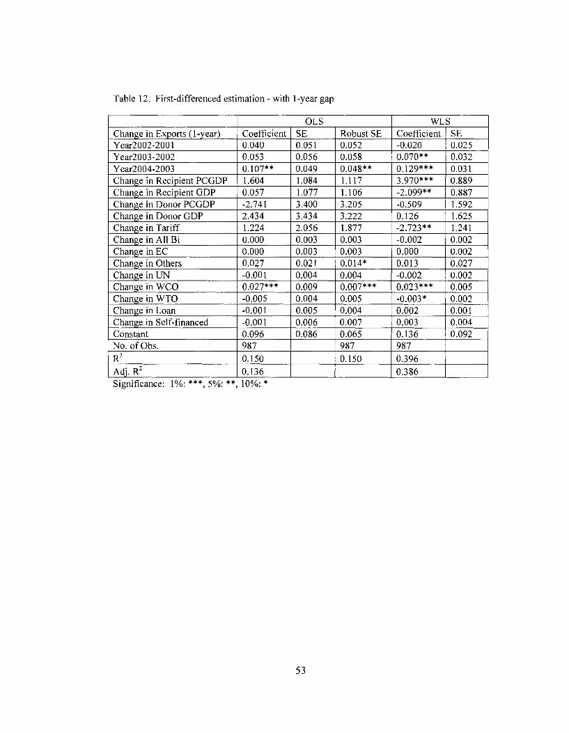
Table 12. First-differenced estimation - with I-year gap

Significance: 1%: ***, 5%: **, 10%: *

Table 13. First-differenced estimation - with 5-year gap

Change in Exports (5-year) Change in Recipient PCGDP Change in Recipient GDP Change in Donor PCGDP Change in Donor GDP Change in Tariff Change in All Bi Change in EC Change in Others Change in UN Change in WCO

OLS

2.289 -5.478 -0.018 0.012*

Change in WTO Change in Loan Change in Self-financed

Adi. R2 1 0.331 I I 1 0.686 I I

Coefficient 0.793 0.78 1 -2.197

WLS

0.010 -0.041 0.02 1

Constant 1 0.126 1 0.251 1 0.303 1 0.462* 1 0.272

I

Significance: 1%: ***, 5%: **, 10%: *

Coefficient 2.500*** -0.837 -1.157

2.430 4.203 0.019 0.006

-0.014 0.015** -0.007

No. of Obs. 1 247

SE 0.810 0.757 1.248

SE 0.857 0.818 2.384

0.010 0.031 0.015

1 247 1 247

Robust SE 0.871 0.856 2.425 2.471 4.977 0.021 0.007*

0.015 0.007 0.010

0.009 0.052 0.018

1.042 -5.529** -0.028 -0.004

0.014 0.007** 0.010

1.297 2.335 0.019 0.005

0.015** -0.049 0.041***

0.007 0.045 0.010

-0.034*** 0.009** 0.006

0.010 0.004 0.008

Bibliography

Aitken Norman D. "The effect of the EEC and EFTA on European trade: A temporal cross-section analysis." American Economic Review, Dec 1973, 63(5), 88 1-892.

Aitken, Norman D. and Obutelewicz, R. S. "A cross-sectional study of EEC trade with the association of African countries." Review of Economics and Statistics. 1976, LVIII (4), 425-33.

Anderson, James E. 1979. "A Theoretical Foundation for the Gravity Equation." American Economic Review, March 1979, 69, 106- 1 1 6.

Anderson, James E. and van Wincoop, Eric. "Gravity with Gravitas: A Solution to the Border Puzzle." American Economic Review, March 2003, 93(1), 170-1 92.

Balassa, Bela. "Trade Creation and Trade Diversion in the EEC." Economic Journal, March 1967, 77, 1-21.

Beckerman W. "Distance and the Pattern of Intra-European Trade." Review of Economics and Statistics, February 1956, 38(1), 31-40.

Bergstrand, Jeffrey H. "The Gravity Equation in International Trade: Some Microeconomic Foundations and Empirical Evidence." Review of Economics and Statistics, August 1985, 67(3), 474-81.

Bergstrand, Jeffrey H. "The Generalized Gravity Equation, Monopolistic Competition, and the Factor-Proportions Theory in International Trade." Review of Economics and Statistics, February 1989, 71(1), 143-53.

Bergstrand, Jeffrey H. "The Heckscher-Ohlin-Samuelson Model, the Linder Hypothesis and the Determinants of Bilateral Intra-Industry Trade." Economic Journal, December 1990, 1 OO(403), 12 16-29.

Chenery, Hollis B. "Patterns of industrial growth." American Economic Review, September 1960,50(4), 624-654.

Cyrus, Teresa L. "Income in the gravity model of bilateral trade: does endogeneity matter?" International Trade Journal, 2002, l6(2), 16 1 - 180.

Deardorff, Alan V. "The General Validity of the Heckscher-Ohlin Theorem." American Economic Review, September l982,72(4), 683-694

Finger, J. M and Yeats, A.J. "Effective Protection by Transportation Costs and Tariffs: A Comparison of Magnitudes." Quarterly Journal of Economics, February 1976, 90(1), 169-176.

Frankel, Jeffrey A. and Wei, Shang J. "Trading blocs and currency blocs." National Bureau of Economic Research, NBER Working Papers: 4335, 1993.

Frankel, J., Stein, E., and Wei, S. J. "Trading Blocs and the Americas: The Natural, the Unnatural, and the Supernatural." Journal of Development Economics, June 1995, 47(1), 61-95.

Geraci, Vincent J and Prewo, Wilfried. "Bilateral Trade Flows and Transport Costs." Review of Economics and Statistics, February 1977, 59(1), 67-74.

Helpman, E. (1981). "International trade in the presence of product differentiation, economics of scale and monopolistic competition: a Chamberlin-Heckscher-Ohlin approach." Journal of International Economics, 1981, 1 1, 305-40.

Helpman, E. and Krugman, P. Market Structure and Foreign Trade. Cambridge, Massachusetts: MIT Press, 1985.

Hans Linnemann, An Econometric Study of International Trade Flows, Amsterdam 1966.

Isard, Walter and Peck, Merton J. "Location Theory and International and Interregional Trade Theory." Quarterly Journal of Economics, February 1954,68 (1), 97-1 14.

Isard, Walter. "Location Theory and Trade Theory: Short-Run Analysis." Quarterly Journal of Economics, May 1954,68(2), 305-320.

Linnemannn, Hans. An Econometric Study of International Trade Flows, Amsterdam, Netherlands: North-Holland, 1966.

McCallum, John. "National Borders Matter: Canada-U.S. Regional Trade Patterns." American Economic Review, June 1995, 85(3), 61 5-23.

Moneta, Carmellah. "The Estimation of Transportation Costs in International Trade." Journal of Political Economy, February 1959, 67(1), 4 1-58.

Oguledo, Victor I and MacPhee, Craig R. "Gravity models: a reformulation and an application to discriminatory trade arrangements." Applied Economics , February 1994, 26(2): 107- 120.

Pelzman, Joseph. "Trade creation and trade diversion in the Council of Mutual Economic Assistance: 1954-70", American Economic Review, September 1977, 67(4), 71 3- 722.

Poyhonen Pentti. "A tentative model for the volume of trade between countries. Weltwirtschaftliches Archive, 1963, 90, 93-99.

Roberts, Benjamin A. "A gravity study of the proposed China-ASEAN free trade area." International Trade Journal, 2004, l8(4), 335-353.

Thursby, Jerry G. and Thursby, Mary C. "Bilateral trade flows, the Linder hypothesis, and exchange rate risk." Review of Economics and Statistics, August 1987, 69(3), 488-495.

Tinbergen, Jan. "Shaping the World Economy: Suggestions for an International Economic Policy." New York Twentieth Century Fund, 1962.

Wilson, John S., Mann, Catherine L. and Otsuki, Tsunehiro. "Trade Facilitation and Economic Development: Measuring the Impact." World Bank, Policy Research Working Paper Series: 2988,2003.

Wilson, John S., Mann, Catherine L. and Otsuki, Tsunehiro. "Trade Facilitation and Economic Development: A New Approach to Quantifying the Impact." World Bank Economic Review, 2003, 17(3), 367-389.

Wilson, John S., Mann, Catherine L. and Otsuki, Tsunehiro. "Assessing the Potential Benefit of Trade Facilitation: A Global Perspective." World Bank, Policy Research Working Paper Series: 3224, February 2004.

Wilson, John S., Mann, Catherine L. and Otsuki, Tsunehiro. "Assessing the Benefits of Trade Facilitation: A Global Perspective." World Economy, June 2005, 28(6), 841- 871.

Wolf, Charles Jr. and Weinschrott, David. "International Transactions and Regionalism: Distinguishing Insiders from Outsiders." American Economic Review, May 1973, 63(2), 52-60

Woo, Y.P. and Wilson, J. Cutting Through Red Tape, APF Canada, Vancouver, 2000.

Woodridge, J.M. Introductory Econometrics: A Modem Approach. South Western College Publishing, USA, 2000.