bulent eris model development for planning and forecasting in diagnostic and treatment systems...
TRANSCRIPT
8/8/2019 Bulent Eris Model Development for Planning and Forecasting in Diagnostic and Treatment Systems 9022004
http://slidepdf.com/reader/full/bulent-eris-model-development-for-planning-and-forecasting-in-diagnostic-and 1/182
T.C.MARMARA UNIVERSITY
INSTITUTE FOR GRADUATE STUDIES INPURE AND APPLIED SCIENCES
MODEL DEVELOPMENT FOR PLANNING ANDFORECASTING IN DIAGNOSTIC AND TREATMENT
SYSTEMS
Salih Bülent ER ŞMSc.(Management Engineering)
THESISFOR THE DEGREE OF DOCTOR OF PHILOSOPHY
ININDUSTRIAL ENGINEERING
SUPERVISOR
Prof.Dr. Erkan TÜRE
STANBUL 2004

8/8/2019 Bulent Eris Model Development for Planning and Forecasting in Diagnostic and Treatment Systems 9022004
http://slidepdf.com/reader/full/bulent-eris-model-development-for-planning-and-forecasting-in-diagnostic-and 2/182
T.C.MARMARA UNIVERSITY
INSTITUTE FOR GRADUATE STUDIES INPURE AND APPLIED SCIENCES
MODEL DEVELOPMENT FOR PLANNING ANDFORECASTING IN DIAGNOSTIC AND TREATMENT
SYSTEMS
Salih Bülent ER ŞMSc.(1412009 19920009)
THESISFOR THE DEGREE OF DOCTOR OF PHILOSOPHY
ININDUSTRIAL ENGINEERING
SUPERVISOR
Prof.Dr. Erkan TÜRE
STANBUL 2004

8/8/2019 Bulent Eris Model Development for Planning and Forecasting in Diagnostic and Treatment Systems 9022004
http://slidepdf.com/reader/full/bulent-eris-model-development-for-planning-and-forecasting-in-diagnostic-and 3/182
ACKNOWLEDGEMENTS
I would like to express my sincere gratitude to my thesis advisor, Prof. Dr. ErkanTüre, for his supervision, guidance, continued support and motivation throughout this study.
I wish to extend my thanks and Prof Dr. Sevil Ünal, Prof Dr. Sami Ercan, Prof. Dr.
Taylan Ula and Asst. Prof. Dr Güldal Büyükdamgacı for serving on my thesis committee and
for their valuable advices and comments.
Special appreciation is due to my General Manager Asst. Prof. Dr. Giray Velioğlu,
and Asst. General Manager Umur Çullu and my colleagues Burak Sayın, Deniz Sümengen,Esra Güler, Ulas Öncül, Ercan Tekin, Utku Birdal and Ali Özmen for their valuable technical
advice.
Finally, I would like to thank to my wife Nalan and son Onat for their patience,
encouragement and support
Eylül, 2003 Salih Bülent Eriş

8/8/2019 Bulent Eris Model Development for Planning and Forecasting in Diagnostic and Treatment Systems 9022004
http://slidepdf.com/reader/full/bulent-eris-model-development-for-planning-and-forecasting-in-diagnostic-and 4/182
TABLE OF CONTENTS
ACKNOWLEDGEMENTS.................................................I
TABLE OF CONTENTS....................................................II
ÖZET ..........................................................................................V
ABSTRACT .....................................................................................VI
ORIGINALITY CLAIM..................................................VII
LIST OF SYMBOLS............................................................. X
ABBREVATIONS..................................................................XI
LIST OF FIGURES............................................................XII
LIST OF TABLES..............................................................XIV
PART.I. INTRODUCTION AND OBJECTIVES ......................1
PART.II. GENERAL BACKGROUND ........................................4
II.1 PRIVATE HEALTH INSURANCE IN THE WORLD .......................4
II.2 TURKEY PRIVATE HEALTH INSURANCE BACKGROUND.......7
II.3 HEALTH RISK MODELS IN LITERATURE..................................11
II.3.1 Demographic Models .......................................................12
II.3.2 Prior Year Expenditures ...................................................14II.3.3 Diagnosis-Based Risk Adjustment....................................15
II.3.4 Information Derived from Prescription Drugs...................17
II.3.5 Self-Reported Health Information.....................................17
II.3.6 Mortality..........................................................................18

8/8/2019 Bulent Eris Model Development for Planning and Forecasting in Diagnostic and Treatment Systems 9022004
http://slidepdf.com/reader/full/bulent-eris-model-development-for-planning-and-forecasting-in-diagnostic-and 5/182
II.3.7 Other Models ...................................................................18
II.4 PRIVATE HEALTH INSURANCE PRICING .................................18
II.4.1 Practice of Pricing in the World........................................18
II.4.2 Theory of Health Insurance Pricing ..................................23
PART.III. ANALYSIS OF THE DATA........................................26
III.1 DIAGNOSIS AND TREATMENT SERVICES CATEGORIES.......27
III.1.1 Out- patient Treatment (without hospitalization) ............27
III.1.2 In-patient Treatment.............. ..........................................28
III.2 ESTIMATION OF PARAMETERS .................................................29
III.2.1 Prior year stats ................................................................30
III.2.2 Group size.......................................................................33
III.2.3 Parameters .............................................. ........................37
III.3 MOMENTS OF USAGE ..................................................................43
III.3.1 Comparison of the Data from Other Sources ...................50
PART.IV. THE MODEL................................................................52
IV.1 ALTERNATIVE MODELS..............................................................52
IV.1.1 Moments Based Approach ..............................................52
IV.1.2 Recursive Algorithm.......................................................55
IV.1.3 Inversion -Methods Fast Fourier- ....................................55
IV.2 SIMULATION MODEL STRUCTURE...........................................57
IV.2.1 Individual Expenses Module...........................................58IV.2.1.1 Pc, n, X 61 IV.2.1.2 Age and Gender 61 IV.2.1.3 Distribution Assumptions 61 IV.2.1.4 Limits and Deductibles 63 IV.2.1.5 Dependency 66 IV.2.1.6 Short Term Monthly Analysis 68
IV.2.2 Experience - Credibility Module .....................................75IV.2.2.1 Experience Rating with monthly and Quarter Yearly Periods 80
IV.2.3 Individual to Group Module............................................81
IV.2.4 Characteristics of the Model Output and Sensitivity........83IV.2.4.1 The Effect of Dependency 84 IV.2.4.2 The Effect of Group Size and Uncertainty on Individual to Group Module 87 IV.2.4.3 Sensitivity 90
PART.V. IMPLEMENTATION AND MODELVALIDATION ..........................................................95

8/8/2019 Bulent Eris Model Development for Planning and Forecasting in Diagnostic and Treatment Systems 9022004
http://slidepdf.com/reader/full/bulent-eris-model-development-for-planning-and-forecasting-in-diagnostic-and 6/182
V.1 IMPLEMENTATION.......................................................................95
V.1.1 Characteristic of the Sample Data ....................................95V.1.1.1 Age and Gender Profiles 95 V.1.1.2 Profile of Group 1 97 V.1.1.3 Profile of Group 2 97 V.1.1.4 Profile of Group 3 97
V.1.2 Scenarios .........................................................................97V.1.2.1 Output Analysis 99
PART.VI. CONCLUSION ...........................................................139
REFERENCES..............................................................................143
APPENDIX 1..........................................................................146
Definiton of the Actuary.............................................................146
Extreme Cases............................................................................148
APPENDIX 2..........................................................................150
APPENDIX 3..........................................................................157
CURRICULUM VITAE...............................................................161

8/8/2019 Bulent Eris Model Development for Planning and Forecasting in Diagnostic and Treatment Systems 9022004
http://slidepdf.com/reader/full/bulent-eris-model-development-for-planning-and-forecasting-in-diagnostic-and 7/182
ÖZET
TEŞH S VE TEDAV S STEMLER NDE PLANLAMA AMAÇLITAHM NE YÖNELK MODEL GEL ŞT R LMES
Bu çalışmanın amacı ülkemizdeki gerek özel sağlık sigortalarında gerekse sağlık
sandıklarındaki grupların kullanılmak üzere gelecekteki sağlık hizmetlerinden faydalanma
adetleri-miktarları ve maliyetlerini kısa ve orta vadede tahminde kullanılacak dinamik bir
model geliştirilmesidir. Bu çalışma simülasyon modelinin kurulması, duyarlılık analizi ve
7436 kişilik örnekli pilot uygulamalarla sınanmasıyla amaca ulaşmıştır. Güvenilir sonuçlara
ulaşabilmek amacıyla eldeki gerçek verilerden faydalanılarak çeşitli değişkenler
kullanılmıştır.
Geleneksel modellerde sadece grup büyüklüğüne dayanarak limit ve muafiyetinetkilerini göz ardı ettiğinden karşılaşılan risk ve dolayısıyla maliyetlerle ilgili yeterince bilgi
sağlamamaktadır. Bu çalışmada üç modül kullanılmıştır. Bireysel Harcamalar Modülü’nde
değişik yaş cinsiyet dağılımlarından oluşan gruplarda, değişik limit ve muafiyet sonucu ortaya
çıkacak maliyet tahminleri yapılmıştır. Bireysel’den Gruba Modülünde gerçek yaşamda
incelenmesi zor olan değişkenler arası bağımlılığın etkisi, tahmin üzerinde istatistiksel
dalgalanma ve bunların dışındaki, parametre hataları veya verinin uygunluğu gibi
belirsizliklerin etkilerinin nasıl incelenebileceği gösterilmiştir. Grubun önceki harcamalarının
değerlendirilmesi Deneyim-Kredibilite Modülü’nde kullanılmıştır.
Bu çalışmada ayrıca Türkiye’deki Sağlık hizmetleri konusunda ekonomi, ekonometri,
aktüerya ve yöneylem araştırması/endüstri mühendisliği konularında çok az sayıda araştırma
olduğundan tahmin konusundaki araştırmalara geniş olarak yer verilmiştir.
Eylül, 2003 Salih Bülent Eriş
8/8/2019 Bulent Eris Model Development for Planning and Forecasting in Diagnostic and Treatment Systems 9022004
http://slidepdf.com/reader/full/bulent-eris-model-development-for-planning-and-forecasting-in-diagnostic-and 8/182
ABSTRACT
MODEL DEVELOPMENT FOR PLANNING AND FORECASTING INDIAGNOSTIC AND TREATMENT SYSTEMS
In this study we intended to build a dynamic forecasting model for future health care
service costs and utilizations of the groups in the short and mid term ranges in private health
insurance and health funds. This study covers its scope by developing and testing validity of a
simulation model together with the sensitivity analysis and pilot applications on a sample of
7436 people. Real data have been used to describe a model with a number of variables so that
reliable forecasts can be made.
Traditional models that rely on just group size and ignore the effect of limit and
deductibles do not furnish adequate information on the potential risk and therefore the cost
involved. Three different modules have been used. In Individual Expenses Module cost
forecasts for the groups with different age and gender distributions where different limits and
deductibles are done. Factors which can not be tested in real life like interrelational
dependency between variables, statistical fluctuations due to group size, uncertainty due to
credibility and suitability of the data are examined in Individual to Group Module. Group
prior statistics are used in the Experience Rating – Credibility Module.
As there are very few academic or non-academic research studies on economics,econometrics, actuarial or operations research/industrial engineering fields concerning health
care services in Turkey we provided a wide range of literature for forecasting research on
health systems on different disciplines.
September, 2003 Salih Bülent Eriş

8/8/2019 Bulent Eris Model Development for Planning and Forecasting in Diagnostic and Treatment Systems 9022004
http://slidepdf.com/reader/full/bulent-eris-model-development-for-planning-and-forecasting-in-diagnostic-and 9/182
ORIGINALITY CLAIM
MODEL DEVELOPMENT FOR PLANNING AND FORECASTING INDIAGNOSTIC AND TREATMENT SYSTEMS
Health is a dynamic and relative concept both on individual and national base. The
objective of health care systems, their structures, functions, their effectiveness largely differ at
local, regional and national levels. Relations between the elements of the health care systems
and the interaction of these elements with the other elements like cultural behaviors of the
people in the society, environmental conditions etc have complex and dynamic
characteristics.
Strategic health care decision problems including medical, behavioral, socio-economic,
managerial and technical variables can be solved only by integrated and inter disciplinaryapproach. Quantitative techniques and methods have been applied with success for more than
30 years now in finding solutions to the health care decision problems of developed countries.
In Turkey, there is a multi provider health care system which is managed by the
Ministry of Health, social security organizations, armed forces, universities and private
organizations. This system has many problems like over utilization of health care services
leading to the huge health care expenses and budget deficits. Until now the government or the
other parties involved have offered solutions and approaches regarding the political medical,financial and organizational factors. But the approach of mathematical modeling and
prediction techniques that can be employed in health care systems to control the expenditures
and service utilization has been largely ignored .

8/8/2019 Bulent Eris Model Development for Planning and Forecasting in Diagnostic and Treatment Systems 9022004
http://slidepdf.com/reader/full/bulent-eris-model-development-for-planning-and-forecasting-in-diagnostic-and 10/182
The condition stated above is also valid for the insurance sector. When Turkish and big
European Health Insurance markets are observed, it is seen that there is enormous need for
development of forecasting models. It is nearly impossible to find neither detailed academic
studies nor application examples on decision-making and health insurance claims prediction
models. Models should be adaptive and should be suitable for all kinds of health insurance
products. Most of the common approaches in the market are far from supplying flexible
solutions for different health insurance products including various specifications. Simple
common assumptions, pricing and prediction approaches are believed to insufficient and so
they are criticized in this study
The problem in model building in health systems comes from the lack of data and the
uncertainty concerning the model structure, parameters and interrelations between variables.
The complexity (compound and mixed statistical nature of the health utilizations and costs)
makes it harder in addition to issues stated above.
The originality of this study is that it is the first example of a health care expenses
prediction simulation model in group health insurances in Turkish health insurance sector.
The model is purely constructed from the scratch using the actuarial, mathematical and
statistical techniques. The originality also lies in the real insurance claims data which was
derived from the health insurance expenses (claims) made by the insured population building
up the portfolio of a certain insurance company. In this context the data is unique andcontrollable since it is obtained through real observations and a well running IT system.
While building up the model, the stochastic nature of the process is examined and the
distribution characteristics of costs and utilizations in monthly and annual intervals are shown
depending on the real data.
The model has 3 different modules as follows;
A- Individual Expense Module: This module reduces the group medical expensesbehavior to individual and creates a representative individual expense form on an expense
type basis. The module variables are set as; probability of claiming (Pc), number of claims(n),
claim size(X) for demographical classes. Setting these variables is a new approach that allows
the usage of positively skewed or long tailed non-zero distributions, which are allocated to
severity and frequency of variables.

8/8/2019 Bulent Eris Model Development for Planning and Forecasting in Diagnostic and Treatment Systems 9022004
http://slidepdf.com/reader/full/bulent-eris-model-development-for-planning-and-forecasting-in-diagnostic-and 11/182
B-Experience and Credibility Module: This module combines the observed results of
the examined groups’ statistics with the standard portfolio values to improve the estimation.
This is done for the distributional characteristics of each utilization type (physician visit
prescribed drugs, etc) for each variable of the model (Pc, n and X). This is also another new
proposal to the actuarial study ground where the actuarial health studies are rarely
sophisticated.
C-Individual to Group Module: Taking into account the group size and the uncertainty
from other factors (trend, credibility and suitability of the data), this module examines the
possible variations on the empirical distribution output from the A and B modules to quantify
the stochastic nature. This prediction of uncertainty approach is also new to Turkish health
insurance sector.
The model presented in this study is a potentially useful tool for either private insurance
companies (which have approximately 700,000 insured) or health aid funds (which have more
than 270,000 members) in Turkey. The companies or health aid funds can determine the
distribution characteristics of health care needs for populations that are formed of people in
different age and gender groups. The suggested methods could also be used for social security
or governmental planning purposes when the data is based on a short-term period.
September, 2003 Prof.Dr. Erkan TÜRE Salih Bülent Eriş

8/8/2019 Bulent Eris Model Development for Planning and Forecasting in Diagnostic and Treatment Systems 9022004
http://slidepdf.com/reader/full/bulent-eris-model-development-for-planning-and-forecasting-in-diagnostic-and 12/182
LIST OF SYMBOLS
n :Claim Count(utilization of the observed health care service)
Pc :Probability of claimingX :Cost of the utilized health care service
αααα , λλλλ :Parameters of Gamma and Pareto distributions
σσσσ :Population STD
1 X φ :The characteristic functions of the input distributions
ω :The correlation matrix for two different benefits
γ γγ γ : Skewness
Z : Credibility

8/8/2019 Bulent Eris Model Development for Planning and Forecasting in Diagnostic and Treatment Systems 9022004
http://slidepdf.com/reader/full/bulent-eris-model-development-for-planning-and-forecasting-in-diagnostic-and 13/182
ABBREVATIONS
MSA : Medical Saving Accounts
MCO : Managed Care Organization
LER : Loss Elimination RatioLEV : Limited Expected Value
ACG : Ambulatory Care Group
DCG : Diagnostic Cost Group
DPS : Disability Payment System
HCC : Hierarchical Condition Categories.
ICD : International Classification of Diseases
CDS : Chronic Disease Score
NHE : National Health ExpenditureCPI : Consumer Price Increases
NCD: : No Claim Discount
RF: Rating Factors
PMPM: Per Member Per Month

8/8/2019 Bulent Eris Model Development for Planning and Forecasting in Diagnostic and Treatment Systems 9022004
http://slidepdf.com/reader/full/bulent-eris-model-development-for-planning-and-forecasting-in-diagnostic-and 14/182
LIST OF FIGURES
Figure II.1 Health Spending for Gender, Age Sample Netherlands........................................13
Figure II.2 Health Spending for Gender, Age Sample USA Privately Insureds......................13
Figure II.3 Health Spending for Gender, Age Sample USA Medicaid Eligibles ....................13Figure II.4 Distribution of population costs to the members for year one and two .................14
Figure II.5 Group and Individual Rating Structures ..............................................................19
Figure II.6 Distribution of Relative Costs Between Groups...................................................22
Figure III.1 Ratio of Users to the Population.........................................................................37
Figure III.2 Ratio of Physician Users in Age and Gender Band Population ...........................38
Figure III.3 Average Number of Visits for Different Age and Gender Bands ........................38
Figure III.4 Distribution of Number of Visits for Different Age and Gender Bands ..............39
Figure III.5 Average Cost Per Usage ....................................................................................39Figure III.6 Distribution of Visit Costs for Different Age and Gender Bands ........................40
Figure III.7 Gender and age effect on sample data ................................................................42
Figure IV.1 Output for Prescribed Drugs of a Group.............................................................56
Figure IV.2 Second Fourier Example....................................................................................57
Figure IV.3 Creation of the Input Parameters for Individual to Group Module + Experience-
Credibility Module........................................................................................................59
Figure IV.4 Iteration of the Individual Expense Module(fed with credibility if any) .............60
Figure IV.5 Hospital Claim Cost X graph produced with gamma and real data.....................62
Figure IV.6 Number of Physician Visits n graph produced with gamma and real data...........62
Figure IV.7 Limit and Deductible Application Process ................................. ........................64
Figure IV.8 Limit and Deductible Affect On Diagnostic Annual Costs.................................65
Figure IV.9 When various scenarios Applied Total Costs on Individual Basis ......................66
Figure IV.10 Development of Distributions..........................................................................69

8/8/2019 Bulent Eris Model Development for Planning and Forecasting in Diagnostic and Treatment Systems 9022004
http://slidepdf.com/reader/full/bulent-eris-model-development-for-planning-and-forecasting-in-diagnostic-and 15/182
Figure IV.11 Distribution of "n" in March and August..........................................................70
Figure IV.12 Flow Process for the Individual to Group Module............................................83
Figure IV.13 Std B coefficients for Total Costs Incurred ......................................................91
Figure IV.14 Std B coefficients for Total Costs After the Limits and Deductibles.................93
Figure V.1Graph of Group 1 Total Costs ............................................................................101
Figure V.2 Graph of Group 1 After First Scenario .............................................................104
Figure V.3 Graph of Group 1 After Second Scenario.........................................................108
Figure V.4 Graph of Group 2 Total Costs ...........................................................................110
Figure V.5 Graph of Group 2 After First Scenario .............................................................113
Figure V.6 Graph of Group 2 After Second Scenario.........................................................117
Figure V.7 Graph of Group 3 Total Costs ...........................................................................119
Figure V.8 Graph of Group 3 After First Scenario .............................................................122
Figure V.9 Graph of Group 3 After Second Scenario..........................................................126
Figure V.10 Physician Visit Comparison ............................................................................130
Figure V.11 Prescribed Drug Comparison ..........................................................................132
Figure V.12 Diagnostic procedure comparison ...................................................................134
Figure V.13 Minor treatment comparison ...........................................................................136
Figure V.14 Hospital benefit comparison............................................................................138

8/8/2019 Bulent Eris Model Development for Planning and Forecasting in Diagnostic and Treatment Systems 9022004
http://slidepdf.com/reader/full/bulent-eris-model-development-for-planning-and-forecasting-in-diagnostic-and 16/182
LIST OF TABLES
Table II-1 Types of VHI in the EU .........................................................................................5
Table II-2 VHI coverage in the EU in 1998 ................................ ............................................5
Table II-3 VHI expenditure as a percentage of total expenditure on health in the EU, 1980-
1998 ...............................................................................................................................6Table III-1 Out Patient Benefits............................................................................................27
Table III-2 In patient Benefits...............................................................................................28
Table III-3 Descriptive Stats for 2 year sample data in total expenditures .............................30
Table III-4 Regression for 2 year total expenditures..............................................................30
Table III-5 ANOVA for Regression for 2 year total expenditures ................. ........................31
Table III-6 Coefficients of Regression for 2 year total expenditures......................................31
Table III-7 Line Fit Plot For 2 Year Expenditures.................................................................31
Table III-8 Descriptive Stats for 2 year total number of utilizations ......................................32Table III-9 Regression Statistics for 2 year total number of utilizations ................................32
Table III-10 ANOVA for Regression Statistics for 2 year total number of utilizations ..........32
Table III-11 Coefficients for Regression Statistics for 2 year total number of utilizations .....32
Table III-12 Line Fit Plot For 2 Year Utilizations .................................................................33
Table III-13 Descriptive stats of the groups formed of males born between 1960 -1970........34
Table III-14 Different Group Size Characteristics.................................................................35
Table III-15 Single Factor ANOVA......................................................................................35
Table III-16 ANOVA table for different group sizes.............................................................36
Table III-17 Correlation of Average Physician Visits vs Group Size.....................................37
Table III-18 Comparison of Average Expenditures Between the Age Gender Classification.41
Table III-19 Correlation between the Average Figures..........................................................42
Table III-20Moments of Physician(Dr) Visits.......................................................................44
Table III-21 Moments of Prescribed Drugs...........................................................................45

8/8/2019 Bulent Eris Model Development for Planning and Forecasting in Diagnostic and Treatment Systems 9022004
http://slidepdf.com/reader/full/bulent-eris-model-development-for-planning-and-forecasting-in-diagnostic-and 17/182
Table III-22 Moments of Diagnostics ...................................................................................46
Table III-23 Moments of Minor Treatment ................................. ..........................................47
Table III-24 Moments of Hospitalization..............................................................................48
Table III-25 Gamma Parameters for Pc, n and X variables for Physician Visits,...................49
Table III-26 Gamma Parameters for Pc, n and X variables for Prescribed Drugs,..................49
Table III-27 Gamma Parameters for Pc, n and X variables for Diagnostics...........................49
Table III-28 Gamma Parameters for Pc, n and X variables for Minor Treatment,..................49
Table III-29 Annual Number Physician Contacts..................................................................50
Table III-30 Annual Number Hospitalizations .............................................. ........................51
Table III-31 Physician contacts with different level of income..............................................51
Table IV-1 Spearman Rank Correlations For Ratio of User Input Data(Pc)...........................67
Table IV-2 Spearman Rank Correlations For Number of Usage Input Data(n) ......................68
Table IV-3 Descriptive Statistics of Monthly Figures ...........................................................71
Table IV-4 Mann-Whitney U test (two-tailed test) for Monthly Incurred Costs.....................72
Table IV-5 Kolmogorov-Smirnov(two-tailed test) test for Monthly Incurred Costs...............72
Table IV-6 Mann-Whitney's U (two-tailed test) test for Monthly Number of Utilizations .....72
Table IV-7 Empirical Distribution for Number of Utilizations for Out Patient Benefits ........73
Table IV-8 Empirical Distribution for Number of Utilizations for In-Patient Benefits...........74
Table IV-9 Credibility ratings for groups with at least 3 year’s claims history ......................76
Table IV-10 Summary Statistic of the Total Costs Incurred(Independent of the limits) .........84
Table IV-11 Distribution of the Total Costs Incurred(Independent of the limits)...................85Table IV-12 Distribution of the Limit and Deductible Applied Costs With Scenario 2..........86
Table IV-13 Summary Statistics of the Limit and Deductible Applied Costs With Scenario 2
.....................................................................................................................................86
Table IV-14 Statistical Summary for Group Members..........................................................88
Table IV-15 Distribution Output for Group Members...........................................................89
Table IV-1612 Std B coefficients for Total Costs Incurred....................................................92
Table IV-17Std B coefficients for Total Costs After the Limits and Deductibles...................94
Table V-1 Age an Gender characteristics of the Sample Data ...............................................96Table V-2 Dr scenarios.........................................................................................................97
Table V-3 Prescription Scenarios..........................................................................................98
Table V-4 Diagnostic Scenarios............................................................................................98
Table V-5 Minor Treatment Scenarios..................................................................................98
Table V-6 Hospital Scenarios ...............................................................................................98

8/8/2019 Bulent Eris Model Development for Planning and Forecasting in Diagnostic and Treatment Systems 9022004
http://slidepdf.com/reader/full/bulent-eris-model-development-for-planning-and-forecasting-in-diagnostic-and 18/182
Table V-7 Distribution of Group 1 Total Costs ...................................................................100
Table V-8 Descriptive Stats of Group 1 Total Costs............................................................101
Table V-9 Mann-Whitney test for Gr1 Total Costs ............................................................102
Table V-10 Kolmogorov-Smirnov test for Gr1 Total Costs.................................................102
Table V-11 Distribution of Group 1 After First Scenario ...................................................103
Table V-12 Descriptive Stats of Group 1 After First Scenario...................... ......................104
Table V-13 Mann-Whitney test for Gr. 1 Scen.1.................................................................105
Table V-14 Kolmogorov-Smirnov test for Gr.1 and Scen. 1................................................105
Table V-15 Descriptive Stats of Group 1 After Second Scenario ................. ......................106
Table V-16 Distribution of Group 1 After Second Scenario ...............................................107
Table V-17 Mann-Whitney test for Gr. 1 Scen.2.................................................................108
Table V-18 Kolmogorov-Smirnov test for Gr.3 and Scen. 2................................................109
Table V-19 Distribution of Group 2 Total Costs .................................................................109
Table V-20 Descriptive Stats of Group 2 Total Costs..........................................................110
Table V-21 Mann-Whitney test for Gr2 Total Costs ..........................................................111
Table V-22 Kolmogorov-Smirnov test for Gr2 Total Costs.................................................111
Table V-23 Distribution of Group 2 After First Scenario ...................................................112
Table V-24 Descriptive Stats of Group 2 After First Scenario...................... ......................113
Table V-25 Mann-Whitney test for Gr. 2 Scen.1.................................................................114
Table V-26 Kolmogorov-Smirnov test for Gr.2 and Scen. 1................................................114
Table V-27 Descriptive Stats of Group 2 After Second Scenario ................. ......................115Table V-28 Distribution of Group 1 After Second Scenario ...............................................116
Table V-29 Mann-Whitney test for Gr. 1 Scen.2.................................................................117
Table V-30 Kolmogorov-Smirnov test for Gr.3 and Scen. 2................................................118
Table V-31 Distribution of Group 3 Total Costs .................................................................118
Table V-32 Descriptive Stats of Group 3 Total Costs..........................................................119
Table V-33 Mann-Whitney test for Gr3 Total Costs ..........................................................120
Table V-34 Kolmogorov-Smirnov test for Gr3 Total Costs.................................................120
Table V-35 Distribution of Group 3 After First Scenario ...................................................121Table V-36 Descriptive Stats of Group 3 After First Scenario...................... ......................122
Table V-37 Mann-Whitney test for Gr. 3 Scen.1.................................................................123
Table V-38 Kolmogorov-Smirnov test for Gr.3 and Scen. 1................................................123
Table V-39 Descriptive Stats of Group 3 After Second Scenario ................. ......................124
Table V-40 Distribution of Group 3 After Second Scenario ...............................................125
8/8/2019 Bulent Eris Model Development for Planning and Forecasting in Diagnostic and Treatment Systems 9022004
http://slidepdf.com/reader/full/bulent-eris-model-development-for-planning-and-forecasting-in-diagnostic-and 19/182
Table V-41 Mann-Whitney test for Gr. 3 Scen.2.................................................................126
Table V-42 Kolmogorov-Smirnov test for Gr.3 and Scen. 2................................................127
Table V-43 F testf or Physician Simulation and real data comparison.................................128
Table V-44 t testf or Physician Simulation and real data comparison ..................................129
Table V-45 F testf or Prescribed Drugs Simulation and real data comparison .....................130
Table V-46 t testf or Prescribed Drugs Simulation and real data comparison ......................131
Table V-47 F testf or Diagnostic Simulation and real data comparison ...............................132
Table V-48 t testf or Diagnostic Simulation and real data comparison ................................133
Table V-49 F testf or Minor Treatment Simulation and real data comparison......................134
Table V-50 t test f or Diagnostic Simulation and real data comparison ...............................135
Table V-51 F testf or Hospital Simulation and real data comparison...................................136
Table V-52 t testf or Hospital Simulation and real data comparison....................................137
Table 0-1 Earthquake predictions from the California Data.................................................148
Table 0-2 Real Earthquake data ................................ ..........................................................148
Table 0-3 High costs incidence rates...................................................................................149

8/8/2019 Bulent Eris Model Development for Planning and Forecasting in Diagnostic and Treatment Systems 9022004
http://slidepdf.com/reader/full/bulent-eris-model-development-for-planning-and-forecasting-in-diagnostic-and 20/182
PART.I.
INTRODUCTION AND OBJECTIVES
Turkey is the third most populous country in World Health Organization’s European
Region, and its economy is among the ten largest in Europe. It has a high growth rate and ayoung population. Turkey is also a candidate for membership of the European Union.
However, the population’s health status and the quality of the health care system are far below
the country’s general level of development.
The last few years have seen a rapid expansion of the private health care sector in
Turkey. The expectations of those with high incomes (last decade has created a high-income
group of between six and eight million people) provide incentives for further expansion and
encourage the private sector to play a larger role in the health care system. Furthermore
patients prefer private to public health care, regardless of their income, due to a lack of
confidence in public health services and a belief that private health care is of better quality
It is difficult to make reliable estimates of the extent of out-of-pocket payments in
Turkey, as private spending on health care is not well documented. Official sources like the
World Health Organization’s European health for all database records, The Organization for
Economic Co-operation and Development (OECD), and reports of the Ministry of Health puts
the percentage of out of pocket expenses to be 28% of all health care expenditures which is 10
billion USD in official figures. This constitutes a total expenditure of 3 billion USD with out
of the record expenses. Taking into account differences in the relative purchasing power of
various currencies, Turkey’s GDP per capita (Intl $) is 6,455 where the total health
expenditure per capita (Intl $) is 323. ( in normal USD currency it is approximately GDP is
2000$ and expenditure is 110$) When we compare health care expenditures with other

8/8/2019 Bulent Eris Model Development for Planning and Forecasting in Diagnostic and Treatment Systems 9022004
http://slidepdf.com/reader/full/bulent-eris-model-development-for-planning-and-forecasting-in-diagnostic-and 21/182
comparable countries like Hungary (846$, 24.3 % of this is private expenditure), Greece
(1,390$, 44.5 % of this is private expenditure) we can say that private health care
expenditures are very low and will increase in the following years due to the technological
progress, the new expectations of consumers, population aging and the reluctance of
governments to devote an ever-growing proportion of State budget.
Private health insurance always plays a complementary role, which varies in
significance, in the majority of the countries all over the world. In some countries private
insurance even has partially taken the place of public services. Private insurance plays its role
at two different levels: the financing level, where the insurer reimburses the cost of care or
provides compensation, and the care providing level such as in the case of managed care. So
private health insurance covers a very extensive range of services, and also brings into play
many different operators. Its characteristics, and in particular the extent of its integration in
the various parts of the public systems, differ considerably from one country to another.
Considering the Private Health Care Expenditures covered by private health insurance
in Turkey, (257 Trillion TL which is 170 million USD) and covered population to be 700,000
which is 1% of population) if the system grows like in the western countries then the insured
population will grow to 10 million and will be covering privately insured expenses totaling
more than 2 Billion USD comparatively .
In private health insurance, contracts are done as a group or individually. In group
contracts employers or unions are contracting with the private health insurance company. But
for individual contracts, people are paying for their families. Because of the higher risk of
adverse selection for the insurance company, the conditions are much more stricter and
premium is higher for individual contract than group contracts.
To avoid major inequalities or excessive rise in premiums, group insurance contracts
have been favored by the regulation in the countries where private medical insurance is welldeveloped. And as a result of this group contracts are widespread in a number of countries. (In
US %70 of the population is covered under group business)
Only in a few countries health insurance statistics are published in sufficient volume to
be credible and meaningful. It is very hard to find the technical literature on private health

8/8/2019 Bulent Eris Model Development for Planning and Forecasting in Diagnostic and Treatment Systems 9022004
http://slidepdf.com/reader/full/bulent-eris-model-development-for-planning-and-forecasting-in-diagnostic-and 22/182
insurance. For example in UK where 11.5% of the population is under private health
insurance, there are no official published statistics as classified in this thesis. Though the
majority of the published actuarial literature is UK origin, first article on health insurance was
written in 1988 and few additional articles were published after that. Due to the lack of
information new articles written in UK still refer to the overseas articles like the ones that are
published in US or Australia.
The objective of this study is to prepare a dynamic forecasting model in private group
health insurance business and health funds. Real data have been used to describe the model
with a large number of variables so that reliable forecasts can be made. Structure of such a
model that aims to reflect a real life situation made up of various distributions with different
characteristics is very complex.
While developing this model, it is aimed to;
· Outline the approaches and adopt some general actuarial concepts to private health
insurance. (Since this is the first example of a health care expenses prediction simulation
model in group health insurances in Turkey.)
· Determine the structure of the model made up of various modules, taking into account
the age and gender differences on utilizations and unit costs, experience of the examined
group previous year statistics, uncertainty due to various factors such as trend, credibility and
suitability of the data.· Test the model due to interrelations and sensitivity of variables.

8/8/2019 Bulent Eris Model Development for Planning and Forecasting in Diagnostic and Treatment Systems 9022004
http://slidepdf.com/reader/full/bulent-eris-model-development-for-planning-and-forecasting-in-diagnostic-and 23/182
PART.II.
GENERAL BACKGROUND
II.1 PRIVATE HEALTH INSURANCE IN THE WORLD
In industrial States, health care financing has historically been inspired by three
competing “models”: the first one, implemented by Bismarck in Germany, relied on
professional enrolment through compulsory contributions from employers and employees;
more recently, Beveridge introduced in the after war UK a public health monopoly, ensuring
universal social protection. The last form of organization is a mix-system, which prevails in
the US, where health insurance is not compulsory [23].
The extend and pace of the development of private health insurance in each country has
been very dependant on the original pattern of the national health care organization, even if
most countries tend to have now a rather hybrid health care system (mixing elements from the
three original models). Amongst OECD member countries, strong contrasts can now be
observed in the balance between private and public health insurance. Although, private sector
is mainly supplementary to public coverage, in some countries it can substitute to public
sector to cover even primary care for all or part of the population. Lastly private health
insurance may provide the same level of coverage than the existing public scheme, whilegiving access to private providers.
According to these regulations, if we would like to explain the systems in EU [23],

8/8/2019 Bulent Eris Model Development for Planning and Forecasting in Diagnostic and Treatment Systems 9022004
http://slidepdf.com/reader/full/bulent-eris-model-development-for-planning-and-forecasting-in-diagnostic-and 24/182
Table II-1 Types of VHI in the EU
Supplementary
increases choice / access
Faster access
increased choice of provider
own room in hospital
Complementary
services excluded / not fully covered
by the state
Dental care
‘alternative’ treatment
co-payments
Substitutive
the principle means of protection
Spain
Germany
Netherlands
Table II-2 VHI coverage in the EU in 1998
Country % populationsubstitutive
% populationcomplementary / supplementary
Austria (hospital expenses) 13
(hospital cash payments) 21
Belgium 30
Denmark 28
Finland (children) 33 / (adults) 10
France (co-payments) 85
(other types of VHI) 20
Germany 8.9
Greece 10
Ireland 42
Italy 5
Lux (active population) 75
Neth 31
Portugal 10
Spain 6.8 10.8
Sweden 0.5
UK 11.5

8/8/2019 Bulent Eris Model Development for Planning and Forecasting in Diagnostic and Treatment Systems 9022004
http://slidepdf.com/reader/full/bulent-eris-model-development-for-planning-and-forecasting-in-diagnostic-and 25/182
Table II-3 VHI expenditure as a percentage of total expenditure on health in the
EU, 1980-1998
Country 1980 1985 1990 1995 1998Austria 7.6 9.8 9.0 7.8 7.1
Belgium 0.8 1.2 1.6 1.9 *2.0
Denmark 0.8 0.8 1.3 1.2 1.5
Finland 1.4 1.8 2.2 2.4 2.7
France - 5.8 11.2 11.7 12.2
Germany 5.9 6.5 7.2 6.7 **6.9
Greece - - 0.9 - -
Ireland - - - - 9.4
Italy 0.2 0.5 0.9 1.3 **1.3
Luxembourg - 1.6 1.4 1.4 **1.6
Netherlands - 11.2 12.1 - 17.7
Portugal - 0.2 0.8 1.4 **1.7
Spain 3.2 3.7 3.7 5.2 **1.5
Sweden - - - - -
UK 1.3 2.5 3.3 3.2 3.5
Health care expenditures can be financed according to three basic models: risk-based
calculation of premium, community rating and funding.
Risk based calculation is the most common way for private insurers to provide health
products. Two different types of policies may be distinguished: individual and group
insurance. These models involve different kind of selectivity and premium calculations.
Individual policies are scarce in OECD countries (except in Italy and in Denmark). For
such policies, individual contract premiums are calculated on risk-based criteria such as age
or age at entry, sometimes gender (Luxembourg, Portugal, Switzerland) and often health
status. Therefore premiums are higher for older and weaker persons. Moreover, private

8/8/2019 Bulent Eris Model Development for Planning and Forecasting in Diagnostic and Treatment Systems 9022004
http://slidepdf.com/reader/full/bulent-eris-model-development-for-planning-and-forecasting-in-diagnostic-and 26/182
insurers are allowed in most case to deny the access to high-risked individuals or to impose
waiting period (such as in the US, Luxembourg or Switzerland). This is the case in nearly all
OECD countries except when policies are aimed at protecting specific categories of persons.
Group insurance policies are more common. They are widespread in a number of
countries such as:
The US, with more than 70% of the population covered by this type of scheme,
France, where two thirds of insured are covered by a global contracts through the
employer,
Germany,
The UK, where three quarters of the population have a supplementary health insurance
cover,
Canada,
And recently Portugal, in which 90% of contracts are group insurance policies.
Reasons for this development certainly lie on the particular financial and access
facilities of these policies. Actually, since risks are borne by more people, insured enjoy lower
premiums based on an experience-rated calculation. Insurers may therefore have fewer
incentives to have recourse to risk selection.
II.2 TURKEY PRIVATE HEALTH INSURANCE BACKGROUND
In essence, private health insurance started to develop circa 1990 by offering per event
limited out-patient based policies with a limited surgery, room and board benefits(Health
Insurance is defined to be a separate branch by 1990).
As many multinational companies started investing in Turkey and as a policy they
require Group Health Covers for their employees, private insurance companies have begun to
take part in the health market.
As a result of the lack of confidence to the social security system, the private insurance
companies have developed policies for individuals in addition to policies providing group
health coverage which are being spread out by the help of direct sales teams, and most

8/8/2019 Bulent Eris Model Development for Planning and Forecasting in Diagnostic and Treatment Systems 9022004
http://slidepdf.com/reader/full/bulent-eris-model-development-for-planning-and-forecasting-in-diagnostic-and 27/182
policyholders, although being at the same time contributors to the social security system,
more and more they stopped using the services provided by the social security institutions.
Between 1990 and 1993, as a consequence of the insufficient understanding of
principles of health insurance, health insurance policies were mostly out-patient oriented and
were insufficient for in-patient benefits. In 1994, the benefit structure of these policies was
changed to ones in which more comprehensive in-patient benefits were provided.
Between 1993 & 1995, a serious increase in the private health organizations was
observed. With these modern hospitals, there came a professional approach to private health
insurance. For example, Bayındır Hospital which was owned by a group who has also a life
insurance company, produced a Preferred Provider Organization (PPO) product to sell to the
upper and middle class markets in Ankara. This hospital has established contacts with the
health insurers of Istanbul in 1994.
PPO agreements were done with some of the well known hospitals in Istanbul and in
Ankara by Halk Yaşam and Koç-Allianz Hayat which were the first companies to initiate
PPO concept to the market through the end of 1994.
The leading companies in the market aim to expand this system gradually to the whole
country and thus create a private health service system. These products offer unlimitedbenefits with some exclusions and cost containment measures. Even though the policy is
unlimited, when the insured wants to get service from another provider (non-PPO) then, a
maximum limit, deductibles or coinsurance are applied. But for the emergency cases, when
someone could not reach a PPO, this condition is usually not enforced.
Due to the development in the private health insurance industry, Munich-Re, the most
known foreign reinsurance company in Turkish insurance market established Med-Net system
with foreign partners (a Third Party Administration) in 1994, which was a new concept for theinsurance sector. Small companies prefer this system because policy related services such as
underwriting, policy issuing, premium collections and claim settlements are done by Med-
Net. Med-Net offers a wide range of plans which are equipped with different geographical
scopes, limits, co-insurance and deductibles.

8/8/2019 Bulent Eris Model Development for Planning and Forecasting in Diagnostic and Treatment Systems 9022004
http://slidepdf.com/reader/full/bulent-eris-model-development-for-planning-and-forecasting-in-diagnostic-and 28/182
In 1994, affordable check-up benefits started to be offered by policies.
In 1993 and 1994, insurance companies began to provide air ambulance services which
are not unfortunately being able to be used efficiently. Air ambulances are employed
according to the distribution of the insureds within big cities. The air ambulance system is
supported by wide spread road ambulance system as well.
Since 1995, many different kinds of products have been introduced to the market, some
of which offer benefit limited products both per prescription, per visit limit and annual limit
per benefit whereas new models with annual maximum limits per person are being developed
as package options. In order to increase market penetration, more attractive policy options are
being developed in the market for the middle class people. As far as product designs are
concerned, the market has been moving from a fee for service model to annual limits and even
to unlimited benefit models. Halk Yaşam and Koç-Allianz Hayat have started a family
physician service including also free laboratory tests and keeping health condition records of
the insureds.
In late 1994 and 1995, guaranteed renewability rights were added to some of the
products of the leading companies in the market and Med-Net.
In 1997, companies which were not satisfied with the service quality and continuousincrease in prices started to quit from the market. Another Third Party Administration
Company named Med-Ex entered the market.
In 2001 Private pension law put the condition for life insurance companies who would
like to serve pension business, segregation of the health business is obliged.
As of 2002, there are approximately 700,000 policyholders in the health branch who are
either individually insured or members of group plans.
As a result of a number of factors including the following, there is an expectation of a
significant growth in health insurance business in Turkey in the coming years:
1. The poor quality of health services offered by the social security system.

8/8/2019 Bulent Eris Model Development for Planning and Forecasting in Diagnostic and Treatment Systems 9022004
http://slidepdf.com/reader/full/bulent-eris-model-development-for-planning-and-forecasting-in-diagnostic-and 29/182
2. The introduction of innovative health products which has already built public
confidence.
3. Increase in income levels.
4. Increased awareness.
5. Regulatory changes requiring separate life insurance companies, which
increased management's focus on health and life insurance.
6. Major developments in the financial sector in Turkey, including debt and
equity capital markets which have enabled diverse investment opportunities for individuals
and institutions for life savings (as opposed to bank deposits and real estate being the only
available investment tools pre-1980). Individuals are now more aware of the value added
provided by institutional fund management by investment professionals.
7. Private sector companies becoming more institutionalized as they transform
from family owned businesses into institutionally held corporations and offer better benefits
to their employees. The increased number of multinational companies establishing a presence
or expanding their existing operations in Turkey is resulting in better added benefits to
employees in the form of group health and life programs.
There is also a series of talks and preparations for a health reform, which include
special proposals to maintain the development in the health sector and health insurance
services. This can be outlined as following:
· to unify the 3 major Social Security Institutions ( SSK, BAG-KUR, Emekli Sandigi )
under a Social Security Finance Institution and to separate the concepts of health care
provision and financing;
· to include the non-insured ( almost 35% of the population ) in the new system;
· to expand the service of the Social Security System with the application of a "Green
Card" which provides free health services for people whose monthly income is equal to less
than 1/3 of the minimum wage;
· to separate the financial control of health and pension funds;· to use a modern accounting system throughout the health sector and to use efficient
financial & actuarial methods;
· to provide a modern information system;
· to encourage the establishment of private hospitals with efficient management and
financial systems in order to increase market competition and to decrease the prices;

8/8/2019 Bulent Eris Model Development for Planning and Forecasting in Diagnostic and Treatment Systems 9022004
http://slidepdf.com/reader/full/bulent-eris-model-development-for-planning-and-forecasting-in-diagnostic-and 30/182
· to enlarge the extent of support investments in the health sector;
Private health insurance companies are also allowed to participate in the
implementation of this program.
It is observed that 4/5 of the private insureds belongs to the upper income class and the
upper middle class. The rest are mainly members of group health insurance plans which are
offered as a fringe benefit by the employers in the private sector. The development of the
market with increasing number of insureds will reduce the risk of anti-selection which shall
lead to more affordable premiums for middle class people [29].
Private health insurance companies in Turkey compete with each other by their quality
of service, policy premiums and product differentiation. Preventive medicine, family
physician system and family planning are going to be popular benefits in order to make
policies more desirable. It is observed that the market tends to be more in oligopolistic
structure during the recent years because of the vast entrance into the market.
II.3 HEALTH RISK MODELS IN LITERATURE
Health care expenditures are characterized both by large random variation as well as
large predictable variation across individuals. Such differences create the potential for large
efficiency gains due to planning, risk reduction from social or private insurance, and raise
important concerns about fairness across individuals with different expected needs for
services. Although each population not only has unique demographic and socioeconomic
characteristics but also a distinct medical signature [35], it is indispensable to use experiences,
data and techniques of the other models.
Considerable research has been conducted on alternative forecasting models in many
countries, using a wide range of information.
Risk adjustment means the use of information to calculate the expected health
expenditures of individual consumers over a fixed interval of time (e.g., a month, quarter, or
year)
8/8/2019 Bulent Eris Model Development for Planning and Forecasting in Diagnostic and Treatment Systems 9022004
http://slidepdf.com/reader/full/bulent-eris-model-development-for-planning-and-forecasting-in-diagnostic-and 31/182
In the United States, actuaries have been slow to accept health-based risk adjustment,
despite its greater accuracy.
According to the demographics only, prior year expenditures, diagnoses, information
derived from prescription drugs, self-reported health and functional health status measures,
mortality, and approaches from the other discipline exist.
While examining these methods it should be noted that it very hard to estimate the
health care spending on individual basis. When the numbers reaches to sufficient size (in risk
adjustment literature it is considered to be more than 5000 members but this number is
defined by the characteristics of the health care system and population) than it becomes
possible to estimate the overall costs of the sample size.
II.3.1 Demographic Models
First data that is used in health estimations are age and sex. When we examine the
worldwide statistics and the Turkish data it is clearly seen that age and sex factors are the
primary factors concerning the health utilization and spending.

8/8/2019 Bulent Eris Model Development for Planning and Forecasting in Diagnostic and Treatment Systems 9022004
http://slidepdf.com/reader/full/bulent-eris-model-development-for-planning-and-forecasting-in-diagnostic-and 32/182
Figure II.1 Health Spending for Gender, Age Sample Netherlands
Figure II.2 Health Spending for Gender, Age Sample USA Privately Insureds
Figure II.3 Health Spending for Gender, Age Sample USA Medicaid Eligibles
Age and sex are easy to document and use for risk adjustment, are fair, and generally
accepted by all parties involved. Because the information is independent of medical care, and
not readily gamed, it appears attractive in terms of incentives. Most serious drawback of age

8/8/2019 Bulent Eris Model Development for Planning and Forecasting in Diagnostic and Treatment Systems 9022004
http://slidepdf.com/reader/full/bulent-eris-model-development-for-planning-and-forecasting-in-diagnostic-and 33/182
and sex as risk adjusters are simply that they are weak predictors of individual expenditures
[31].
II.3.2 Prior Year Expenditures
Because expenditures in one year are correlated with expenditure the following year -
the correlation coefficient for total health expenditures is on the order of .2 to .3 - a simple
proposal has often been made to regress expenditures in year two on year one expenditures
(together with other demographic variables) and use this model for calculating risk-adjusted
payments. Newhouse et. al. [24], Van de Ven and Van Vliet [32] and Ash et al. [5] have all
estimated such models and typically find that spending an extra dollar on health care in year
one "predicts" spending of $0.20 to $0.30 in year two. The R2 from a regression that includes
age, sex and prior year expenditures, is generally estimated to be in the range of .06 to .10. on
individual basis These measures are a substantial improvement over demographic only
models, and comparable to the predictive power achieved by diagnosis-based models or
models that use self-reported health status measures.
In the study that was done by Ash et al. [5]], by examining MED-STAT Market Scan
Research Database, the largest multi source private sector health care database in the United
States, 2.7 million individuals were selected and year 1997 and 1998 results were examined.Below figures were gathered,
Figure II.4 Distribution of population costs to the members for year one and two
This is the distributions of Year- One and Year- Two Cost by Year- one Cost Group,
which means in year one top (in term of health care costs occurred) 0,5% of the population

8/8/2019 Bulent Eris Model Development for Planning and Forecasting in Diagnostic and Treatment Systems 9022004
http://slidepdf.com/reader/full/bulent-eris-model-development-for-planning-and-forecasting-in-diagnostic-and 34/182
had spent %23 of the total population and next year in 1998 this group spent the 8% of the
total health care cost of all. And contrary to this bottom %80 of population had spent %13 of
total costs and next year they spent the %49 of costs. As can be seen top spenders tendency to
pay 2-3 times the average can be recognized easily where the bottom cost %80 has more
volatile nature. This shows us the large random component for the individual figures.
Van de Ven describes that the prior year expenditures or utilization appears to be the
best single predictor(where there is only one predictor in hand) of an individual’s future
health expenditures [31]. But Ash et al.(1998) mentions that prior cost, which was historically
superior to diagnostic information for the purpose of predicting future costs, is no longer
better than the current generation of diagnosis- based risk models for predicting future costs.
In her above-mentioned study diagnostic based methods were slightly superior at identifying
the top group with high costs [5].
II.3.3 Diagnosis-Based Risk Adjustment
Since the early 1980's a considerable amount of research has developed risk adjustment
models that use diagnoses from insurance claims to calculate risk-adjusted payments. In 1997,
the US Congress directed CMS to change the way it paid HMOs that contracted with the
federal government to provide Medicare covered services. [27]
The best-known methods are;
• Ambulatory Care Group (ACG)
• Diagnostic Cost Group (DCG)
• Disability Payment System (DPS)
The starting point for all diagnosis based risk adjustment models is the concept that
certain diagnoses predict of health care expenditures. Each of the three major diagnosis basedmodels begins by identifying a subset of all diagnoses that predict current or subsequent year
resource use. Although the three models differ in how they choose their subset of diagnoses,
each attempts to identify codes that are assigned only for encounters involving a
professionally trained clinician. In particular, diagnoses appearing on laboratory, diagnostic

8/8/2019 Bulent Eris Model Development for Planning and Forecasting in Diagnostic and Treatment Systems 9022004
http://slidepdf.com/reader/full/bulent-eris-model-development-for-planning-and-forecasting-in-diagnostic-and 35/182
testing, and medical supplies claims are uniformly not used in classifying individuals for
prediction, on the grounds that they are less reliable than those assigned by clinicians.
ACGs are based on aggregation of all ICD9-CM codes into 32 diagnostic groups using
ambulatory diagnoses only. These diagnostic groups can then be used in a number of
alternative combinations, providing up to 83 mutually exclusive ACGs into which any given
individual may be classified.
DCGs have received the most attention of all classification systems. Early versions of
this system were based on simple hierarchical models of diagnosis grouping, where modeling
was used to identify a large number of clinically homogenous groups, which were then
aggregated into between 9 and 20 Diagnosis Cost Groups. The DPS was developed for US
Medicaid disabled enrollees, and is based on similar principles to the DCG/HCC model. All
diagnoses from clinical encounters are used within a hierarchical system for conditions.
However, the DPS is more additive than the DCG/HCC system in its methods to account for
the number of conditions an individual has within certain body systems. The general disability
of the DPS is unclear, however, as its development and application has focused on people
with disabilities.
Also in USA, where medical infrastructure is said to be the technologically foremost
developed one in the world, the systems that combine diagnoses from patient - clinicianencounters across the spectrum of health care delivery sites with age and sex are now being
used by health care organizations to measure the health risk of populations. However, many
organizations have not implement ed “all encounter” diagnosis models because they require
timely, comprehensive, high- quality data from physician’s offices and other dispersed sites of
care.
In USA many author In patient models (diagnosis based) predict next year’s total costs
reasonably well in Medicare, where nearly 20 percent of the population is hospitalizedannually, of ten for chronic conditions. However, such models are less attractive for privately
insured under 65 populations, where fewer than 5 percent are hospitalized in a year and of ten
for acute conditions. Few previous studies have evaluated inpatient diagnosis models on
younger populations. So-called all encounter models that use both inpatient and out patient
diagnoses to predict cost have been developed for several types of populations: elderly

8/8/2019 Bulent Eris Model Development for Planning and Forecasting in Diagnostic and Treatment Systems 9022004
http://slidepdf.com/reader/full/bulent-eris-model-development-for-planning-and-forecasting-in-diagnostic-and 36/182
In Diagnosis based methods the data should be tracked for each member with the
following year costs and the diagnostic codes should be chosen, entered and kept correctly
which is not a very easy situation for Turkish private and social security systems.
II.3.4 Information Derived from Prescription Drugs
A second source of needs measures based on prior utilization is the use of prescription
drugs.
Early work focused on classifying drugs into different therapeutic classes and counting
drug orders in each class. This approach was extended to include clinician judgment of
severity to form weighted disease scores based on outpatient pharmacy utilization and
condition severity to develop the Chronic Disease Score (CDS)
II.3.5 Self-Reported Health Information
Health survey information can be obtained without contact with medical providers, no
prior medical or insurance history is required; reflects individual’s perceptions of their ownneeds and expected utilization, is uniform across health schemes and providers; and other
relevant data, such as socioeconomic measures etc., may also be collected. There are also
disadvantages to self-reported measures of health; surveys are costly to undertake; response
rates may be low and affect the robustness of empirical analysis, requiring large sample sizes;
responses may be correlated with medical risk; reporting may be inaccurate due to errors or
confidentiality issues. Furthermore, provider assistance in conducting surveys may be
required, which may lead to problems in follow up and non-random sampling. Van de Ven
(2000) presents information on the validity of regression models that have sought to explainvariations in health expenditure in terms of health status measures. These studies show that
adding self reported health status measures to demographic variables significantly increases
the predictive power of risk adjustment models. However, self reported health status measures
do not outperform prior diagnosis variables in explaining variations in health expenditure.

8/8/2019 Bulent Eris Model Development for Planning and Forecasting in Diagnostic and Treatment Systems 9022004
http://slidepdf.com/reader/full/bulent-eris-model-development-for-planning-and-forecasting-in-diagnostic-and 37/182
II.3.6 Mortality
In individual level analysis mortality has been proposed as a potential explanatory
variable in regressions on expenditure due to the excess costs incurred prior to death.
However, whether mortality is a useful predictor of variations in expenditure at the individual
level is not clear. One argument is that the costs associated with death are largely
unpredictable, and have been found to be 250% above. A more effective means of
reimbursing health schemes for the costs of death may be to control for deaths in the
regression model (through dummy variables for patients who died during the period, and
reimburse schemes retrospectively for those individuals. Van de Ven (2000) have questioned
the political and social acceptability of increasing payment rates to health schemes with
higher mortality rates. Mortality data may also be poorly coded and only partially available in
some contexts, and may raise some concerns about privacy.
II.3.7 Other Models
There is a considerable literature in statistics, econometrics, and health economics that
examines and assesses alternative functional forms for estimating models of health spending.For data source and applications we recommend [2,3,6,7,9,11,13,19,22,28 and 33]
II.4 PRIVATE HEALTH INSURANCE PRICING
II.4.1 Practice of Pricing in the World
Group business is defined as any collection of individuals who combine to make a
single proposal for uniform Insurance cover. Usually the collected individuals will beemployees in the same company and the employer will pay for the premiums either wholly or
in part. Generally the group will be a discrete definable unit of individuals and the insurer will
look for some minimum take-up rate of the terms offered, if the scheme is voluntary, in order
to limit and-selection.

8/8/2019 Bulent Eris Model Development for Planning and Forecasting in Diagnostic and Treatment Systems 9022004
http://slidepdf.com/reader/full/bulent-eris-model-development-for-planning-and-forecasting-in-diagnostic-and 38/182
Several kinds of product pricing mechanisms exists in health insurance market starting
from fixed price fully insured plans to experience rated plans with minimal stop loss
insurance protection. The options available to group policy holders increase together with the
increase of the employee within the company. Up to 10 employee groups are invariably
covered by fully insured contracts with no waivers on medical underwriting. Groups of more
than 1000 employees are almost invariably experience rated and all medical underwriting is
relinquished(UK, US) [12, 25,26].
The following chart illustrates the different pricing methods that are used in UK for
different sizes of policy [4]
Size of Policy Pricing methods available
Very large group scheme( > 5000 lives)
Large group scheme( > 500 lives)
Small group scheme( > 100-500 lives)
Very small group scheme
Individual Policyholder
C o s t
P l u s
E x p e r i e n c e
R a
t i n g
M i x o
f B o o
k a n
d
E x p e r i e n c e
R a
t i n g
B o o
k R a
t i n g
Figure II.5 Group and Individual Rating Structures
It should be noted that this chart is dependent on the type of cover offered. The chart is
appropriate for a cover including mainly hospital benefits. The size of scheme at which
Experience rating becomes appropriate would reduce for cover within higher frequency of
claiming (for example cover including primary and dental care) and would increase for cover
with a lower frequency of claiming (for example cover including a very large
excess/deductible).(smaller groups can be experience rated for higher frequency benefits like

8/8/2019 Bulent Eris Model Development for Planning and Forecasting in Diagnostic and Treatment Systems 9022004
http://slidepdf.com/reader/full/bulent-eris-model-development-for-planning-and-forecasting-in-diagnostic-and 39/182
for a 100 member group can be experience rated for physician visits while it is hard to give
credibility to the group data for hospital benefits )
The premium quoted by an insurer for new groups will be based on the following
general factors: who will be covered (e.g. employees only, employees plus dependants,
hierarchical status of employees)
• the age profile of the group
• type of product
• the group's past claims experience
• method of payment
• location and occupation might also be considered
If the group has never been covered under Private Health Insurance before, then there
would generally be a calculation based on individual book rates(if so) with an appropriate
discount because it is a group scheme (to allow for the lower anti selection that a group
scheme should bring).
The renewal process will follow the same pattern as outlined above, although the
insurer will have to consider any changes within the group during the previous period of
cover (e.g. increase/decrease of the group membership, change in eligibility criteria, orincrease /Decrease in scale of cover).
• individual policy premiums are generally higher than group premiums as
the risk of anti-selection against the insurer is higher when in individual is
financing has own premium
• Some form of experience rating is usually incorporated in group pricing,
whereas individual business is normally priced on a community rate basisi.e. the premium is assesses pari passu with all other lives in the same risk
cell without reference to individual claims experience
• The larger the group size, the greater the credibility that is placed on the
group's own experience

8/8/2019 Bulent Eris Model Development for Planning and Forecasting in Diagnostic and Treatment Systems 9022004
http://slidepdf.com/reader/full/bulent-eris-model-development-for-planning-and-forecasting-in-diagnostic-and 40/182
• No Claim Discounts (NCDs) are sometimes used for individual and group
business in order to make some allowance for individual claims experience
in the premium rates
• Larger groups (more than 50 employees) are often flat rated according to
benefit class, whereas individual business is almost always age rated
• Additional rating factors are considered when pricing group business e.g.
industry, location, size of group, employer's attitude to his employees'
health
• Large groups frequently self-insure up to a point e.g. 125% of expected
claims cost, and purchase administration and stop-loss insurance from the
insurer.
• Benefits and exclusions are generally similar between group and
individual products
• There is other greater scope for customizing benefits for larger groups to
meet their requirements
In US Industry Rating Factors (RFs) were introduced in the late 1950's in an attempt to
appropriately price each group based on its industry. There are a great many "dynamics"
(other than age/sex and geographic area) that drive a group's claims level. The employer's
contribution level, participation rate, the distribution of employees by collar color, and the
annual employee turnover rate, are a few examples of some of the dynamics involved.
“US has the widest library of the written articles in Group Health Insurance Pricing. First group health policy was issued to Montgomery Ward in 1910”[1]

8/8/2019 Bulent Eris Model Development for Planning and Forecasting in Diagnostic and Treatment Systems 9022004
http://slidepdf.com/reader/full/bulent-eris-model-development-for-planning-and-forecasting-in-diagnostic-and 41/182

8/8/2019 Bulent Eris Model Development for Planning and Forecasting in Diagnostic and Treatment Systems 9022004
http://slidepdf.com/reader/full/bulent-eris-model-development-for-planning-and-forecasting-in-diagnostic-and 42/182
And in the same text distributional models are regarded to be “increasingly
sophisticated”
“but contrary to these developments actuaries continue to use highly simplified models.” [1] .
This practical approaches are some times criticized by some actuaries to be “ancient”
“Over the last 45 years, the advances that have taken place in our world have been mind-boggling to saythe least. However, the sad reality is that the group health insurance industry STILL develops an account's
premiums the same way it did 45 years ago!”[30]
Both in US and UK overall out patient benefits are packaged and most of the models are
based on this benefit structure.
In Turkey excluding few companies (Halk Yaşam was one of them) standard rates are
used to be multiplied with the benefits offered, For example for physician visit benefit limited
by 50$, the premium is calculated by multiplying the limit with fix multiplier (for 20%
coinsurance 1.88 for individual and 3.76 for families. Most of the time deductibles or
different type of limits (like total number of visits etc) are not covered in the models. Most of
the time rule of thump case-by-case evaluations are done. According to group size a discount
is applied like 30% discount for 500 lives covered. (Than the multiplier for physician visits
for 50$ drops to 1.3 for individuals and 2.6 for families. For renewal rates most of the time
100% projection is done according to loss (claims paid)/premium ratio i.e. if the overall claim
/ premium ratio is 150%, for the group of 500 lives with the above limits next year the
physician fee is calculated with 50% increase in premium most of the time regardless of the
new year limits. For example if the group gets the limit as 40$ next year the premium will be
(1.5)(40)(1.88)(0.7) =79$
II.4.2 Theory of Health Insurance Pricing
When we put on limits for number of visits or total costs LEV is used. Well Known
distributions like Gamma and Pareto have exact formulas to calculate these limits and
deductibles.

8/8/2019 Bulent Eris Model Development for Planning and Forecasting in Diagnostic and Treatment Systems 9022004
http://slidepdf.com/reader/full/bulent-eris-model-development-for-planning-and-forecasting-in-diagnostic-and 43/182
If we accept the cost of hospitalization to have a Pareto distribution with parameters
alpha and lambda; the limited expected value formula [17]
[ ] ( )
++
+−+
+−
−=
−
x x
x x x X E
λ λ
λ λ α
λ λ α
α λ
α α
111
;1
Equation II-1
And for Gamma;
[ ] ( ) ( )[ ] x x x x X E λ α λ α λ α ;1;1..; Γ −++Γ = Equation (II-2)
This is accepted as the ladder method to see effect of proposed limit or deductible.
Deductible and limits are the amounts which the below and above claims are not paid by the
insured respectively.
The usage of the graph depends on the area of the graph shows the total amount thatwill be paid by the insurer and the insured.

8/8/2019 Bulent Eris Model Development for Planning and Forecasting in Diagnostic and Treatment Systems 9022004
http://slidepdf.com/reader/full/bulent-eris-model-development-for-planning-and-forecasting-in-diagnostic-and 44/182

8/8/2019 Bulent Eris Model Development for Planning and Forecasting in Diagnostic and Treatment Systems 9022004
http://slidepdf.com/reader/full/bulent-eris-model-development-for-planning-and-forecasting-in-diagnostic-and 45/182
PART.III.
ANALYSIS OF THE DATA
As have seen in preceding chapters, there are various approaches to predict the futurehealth costs/expenditures and utilizations.
“Health care expenditures are characterized both by large random variation as well as
large predictable variation across individuals”. As we have to deal with the data’s available
we should define the data where we have drawn the model structure and available input.
• The first resource is the Halk Yaşam Sigorta Statistics between 1996 and 2000
years covering 140.000 insured lives on the average
• Various world statistics for the missing data and benchmarking
• “Health Service Utilization Survey in Turkey” Ministry of Health, Turkey
When we examine the health expenditures of the population we see that major part of
the total is formed of Outpatient (Physician visits, prescribed drugs, diagnostic procedures and
minor treatment) and Inpatient expenditures where the rest of the expenditures are formed of
Maternity, Dental and Optical costs. We will be examining the outpatient and inpatient costs.
The private insurance data is providing us the major characteristics of the population, but as
this group is a selected group in terms of socio economic characteristics, and requires the
members to be healthy at the start of the first policy year (excluding the newborns and big
group members) we have to examine the above mentioned sources as well. Also as the data is
formed of insufficient for the extremely costly cases like organ transplantation we have to get

8/8/2019 Bulent Eris Model Development for Planning and Forecasting in Diagnostic and Treatment Systems 9022004
http://slidepdf.com/reader/full/bulent-eris-model-development-for-planning-and-forecasting-in-diagnostic-and 46/182
benefit from international statistics. Also catastrophe cases like earthquake will be mentioned
in the final part a special estimation for Istanbul with a rule of thump will be provided.
“Health Service Utilization Survey in Turkey” was carried out to provide baseline
information for formulation of National Health System of Turkey has been done with a
30,155 sample size. The information gathered by this survey can be grouped under two part
which are the determination of the characteristics of the consumers, the second is to sort out
the factors influencing utilization.
III.1 DIAGNOSIS AND TREATMENT SERVICES CATEGORIESDifferent kinds of services are obtained from health service providers.
Diagnosis and treatment services will be examined under the below titles:
III.1.1 Out- patient Treatment (without hospitalization)
Table III-1 Out Patient BenefitsBenefit Definition
Medical Visit Physician examinations and
consultations for diagnosis and
treatmentDrug Prescribed or non-prescribed
drug usage
Diagnosis Laboratory, x-ray, MR, etc.
methods
Minor Medical
Treatment
Injections, etc. treatments

8/8/2019 Bulent Eris Model Development for Planning and Forecasting in Diagnostic and Treatment Systems 9022004
http://slidepdf.com/reader/full/bulent-eris-model-development-for-planning-and-forecasting-in-diagnostic-and 47/182
III.1.2 In-patient Treatment
Table III-2 In patient BenefitsBenefit Definition
Room/Bed Room/meal/
Accommodation in hospital
Operation Operation theatre charges,
operations and related expenses.
Physicians/drug/diagnosi
s
While hospitalization
Maternity Normal/
Caesarean
Various Dressings, blood supply,
bandages, etc.
These service and cost elements show the areas on which the related community made
medical expenditures within the specified period.

8/8/2019 Bulent Eris Model Development for Planning and Forecasting in Diagnostic and Treatment Systems 9022004
http://slidepdf.com/reader/full/bulent-eris-model-development-for-planning-and-forecasting-in-diagnostic-and 48/182
III.2 ESTIMATION OF PARAMETERS
Total utilization numbers and cost for these areas for each of the above-mentioned
classifications are formed of;
Pc: The ratio of people who will use this specific treatment within the defined period (1-
non users ratio) I.e. each year 6 % of the population of a group can be hospitalized where 85%
of the same group can use physicians
n: The frequency of treatment among those who demanded the treatment within the
defined period and the analysis of the related distributions. I.e. people who visits physicians
are experiencing 3.5 visits on the average with a variance of 12.
X: The intensity of demand per treatment (cost/duration/service level) among those whodemanded the treatment within the defined period. I.e. People who are visiting physicians are
paying 30 $ on the average with a variance of 900.
In non life insurance where the casualty branches are very dominant in terms of
actuarial literature, the main variables are derived to be severity and frequency. But
examining the characteristics of the health data, in order to be able to use well known
distributions like Gamma and Pareto we concluded to use three rather than two variables.
These outputs are coming from various distributions, which are affected by various
factors and form these we will be examining the following factors;
• Prior year stats
• Group size
• Age
• Gender
• Socio economic status
Examining the data in hand, we have found similar results that are provided in the
literature survey

8/8/2019 Bulent Eris Model Development for Planning and Forecasting in Diagnostic and Treatment Systems 9022004
http://slidepdf.com/reader/full/bulent-eris-model-development-for-planning-and-forecasting-in-diagnostic-and 49/182
III.2.1 Prior year statsExamining the medical expenses between following year medical experiences shows us
the stochastic nature of health expenditures.
In our first sample 1987 insured population is taken and total medical expenditures forall benefits like physician visits, prescribed drugs, diagnostic procedures etc between two
years are compared. USD conversion is used for correlation analysis of the total expenditures
incurred.
This is a very similar result as in literature survey section under “Prior Year Expenditures”
As in the section when we sort the total adjusted costs of the first year and look for the next
year stats than we see that
Table III-3 Descriptive Stats for 2 year sample data in total expenditures
Correlationbetween
years
Averagehealth
expendituresin year 1(USD)
Averagehealth
expendituresin year 2(USD)
top 0.005 0.53 6,134 2,145top 0.01 0.42 5,027 1,757top 0.05 0.42 3,152 1,004
top 0.10 0.31 2,367 875100% 0.25 502 552
When we do regression analysis it is seen that
Table III-4 Regression for 2 year total expendituresRegression Statistics
Multiple R 0.25R Square 0.06
Adjusted R Square 0.06Standard Error 821.35Observations 1987

8/8/2019 Bulent Eris Model Development for Planning and Forecasting in Diagnostic and Treatment Systems 9022004
http://slidepdf.com/reader/full/bulent-eris-model-development-for-planning-and-forecasting-in-diagnostic-and 50/182

8/8/2019 Bulent Eris Model Development for Planning and Forecasting in Diagnostic and Treatment Systems 9022004
http://slidepdf.com/reader/full/bulent-eris-model-development-for-planning-and-forecasting-in-diagnostic-and 51/182

8/8/2019 Bulent Eris Model Development for Planning and Forecasting in Diagnostic and Treatment Systems 9022004
http://slidepdf.com/reader/full/bulent-eris-model-development-for-planning-and-forecasting-in-diagnostic-and 52/182
Table III-12 Line Fit Plot For 2 Year Utilizations
year 1 Line Fit Plot
0102030405060708090
100
0 100 200
year 1
y e a r
2year 2
Predicted year2
III.2.2 Group sizeIn the Turkish insurance market most of the companies are applying discounts for groups with
large number of members like below.Number Of
Lives Under
Insurance
Discountin Unit
Premium25 551 10
101 15176 20
276 25501 30
751 351000 40
As mentioned earlier and that will be provided in the following sections age and gender
categorization has huge impact on the expenditure behavior (not as single person base but a
group of people with the same gender and age band). In order to eliminate the possibility of

8/8/2019 Bulent Eris Model Development for Planning and Forecasting in Diagnostic and Treatment Systems 9022004
http://slidepdf.com/reader/full/bulent-eris-model-development-for-planning-and-forecasting-in-diagnostic-and 53/182
groups to have different demographic nature, if we draw out the Males with the birth dates
between 1960 and 1970 than, examining the group size will be healthier.
Now there are 169 group of males (1960-1970) with a minimum group size of 20 and
covering a total number of people 16704 lives. Average number of physician visits are
calculated. When we look a the descriptive stats of the groups
Table III-13 Descriptive stats of the groups formed of males born between 1960
-1970avg
Mean 1.462951303
Standard Error 0.048237183Median 1.447916667Mode 1.4Standard Deviation 0.627083383Sample Variance 0.393233569Kurtosis 0.198298942Skewness 0.196612365Range 3.341294783Minimum 0.054054054Maximum 3.395348837
Sum 247.2387702Count 169
The aim of this research is to show that mean health care cost per person does not vary
depending on the size of the insured group. To achieve this purpose we use the institutional
customers data of Halk Yaşam as our sample. The first step we take is to categorize the
companies. The companies can be divided into three main groups according to two different
approaches. For the first approach the categorization is made according to the number of
claimants and groups are formed as small (having 100 or less claimants) medium (100-500
claimants) and large (500 and over claimants). For the second approach the groups formed
according to number of employees insured and they are small (having 100 or less employees),
medium (having 100 to 500 employees) and large (having 500 and more employees). The
next step after categorization is to apply ANOVA procedure to check whether there is a

8/8/2019 Bulent Eris Model Development for Planning and Forecasting in Diagnostic and Treatment Systems 9022004
http://slidepdf.com/reader/full/bulent-eris-model-development-for-planning-and-forecasting-in-diagnostic-and 54/182
significant difference between mean health care costs per person for these groups. As it is
known in order to be able to apply ANOVA the variables we are dealing with must normally
distributed. Since our variable is the mean heath care cost per person for each company,
although mean heath care cost per person(A) has a skewed distribution, central limit theorem
allows us to assume that mean of A is normally distributed. So we have no objection in
applying ANOVA. The mean, variance and standard deviations of each group for the first
approach is given below.
Table III-14 Different Group Size Characteristics1-100 101-500 501+
Mean 58.93391 51.95898 45.29502Variance 2172.165 983.7596 439.9523Standard Deviation 46.60649 31.36494 20.97504
As it can be observed from the above table the means of the groups are close to each
other. However, it is still needed to be assured. At 0,05 level of significance we apply the
ANOVA and output is given below.
H0: Mean claim size per capita is equal for all groups
HA: At least one group has a statistically significantly different Mean claim size per
capita
Table III-15 Single Factor ANOVAANOVA
Source
of
Variation
SS df MS F P-value F crit
BetweenGroups
3553.162 2 1776.581 0.94917 0.387631 3.010442
WithinGroups
1145493 612 1871.721
Total 1149046 614

8/8/2019 Bulent Eris Model Development for Planning and Forecasting in Diagnostic and Treatment Systems 9022004
http://slidepdf.com/reader/full/bulent-eris-model-development-for-planning-and-forecasting-in-diagnostic-and 55/182
Since F(calculated)< F(tabulated) we say that we don’t have enough evidence to reject
the null hypothesis at 0,05 level of significance. In other words at 0,95 confidence level we
can say that the mean heath care cost per capita does not vary depending on the size of the
group insured.
For the second approach we can apply the same procedure and test the same hypothesis.
The data summary of the groups constructed according to the number of employees insured is
given below.
(Normality assumption is considered is tested and chi square Goodness of fit values are found
to be satisfactory )
And finally the ANOVA output is
Table III-16 ANOVA table for different group sizes
ANOVASource
of
Variation
SS df MS F P-value F crit
Between
Groups
8799.179 2 4399.59 2.362931 0.094997 3.010349
WithinGroups
1146943 616 1861.92
Total 1155742 618
The decision is parallel to the one we made for the previous case. At 0,95 confidence
level we don’t have enough evidence against equality of the means. Therefore, we can say
that the size of the group do not have a significant effect on the mean health care cost perperson.
As will be seen on the following sections, the group size effect the stochastic nature of
the average annual cost per person and that’s why(it is not easy to explain to small groups) an

8/8/2019 Bulent Eris Model Development for Planning and Forecasting in Diagnostic and Treatment Systems 9022004
http://slidepdf.com/reader/full/bulent-eris-model-development-for-planning-and-forecasting-in-diagnostic-and 56/182
additional contingency loading should be added according to distribution characteristics of the
expected overall costs,
Also the correlation between group size and average physician visit utilization is as
below.
Table III-17 Correlation of Average Physician Visits vs Group Sizeavg size
avg 1size -0.14586 1
III.2.3 ParametersDeriving the characteristics of these distributions and dealing with and the analysis of
the related distributions and determination of the parameters of this distribution by the various
point estimation methods.
I.e. if we assume that the demographic characteristics are similar, what percent of the
population uses the physicians?
Figure III.1 Ratio of Users to the Population
But if we differentiate between the age and gender classes;

8/8/2019 Bulent Eris Model Development for Planning and Forecasting in Diagnostic and Treatment Systems 9022004
http://slidepdf.com/reader/full/bulent-eris-model-development-for-planning-and-forecasting-in-diagnostic-and 57/182
Figure III.2 Ratio of Physician Users in Age and Gender Band Population
CH is for children, FE is for females and MA is for males. As can be seen the ratio of
usage for the Female on the average is much more than males.
Another measure which is the average number of visit (The frequency of treatment) for theusers
of the physician services (non users are not taken into consideration).
If we show the differentiation according to age and gender;
Figure III.3 Average Number of Visits for Different Age and Gender Bands
If we want the shape of the distributions of these frequencies

8/8/2019 Bulent Eris Model Development for Planning and Forecasting in Diagnostic and Treatment Systems 9022004
http://slidepdf.com/reader/full/bulent-eris-model-development-for-planning-and-forecasting-in-diagnostic-and 58/182
Figure III.4 Distribution of Number of Visits for Different Age and Gender
Bands
Again what is the effect of age and gender difference for the cost of each treatment?
The average figures are as follows;
Figure III.5 Average Cost Per Usage
Again the distribution characteristics are;

8/8/2019 Bulent Eris Model Development for Planning and Forecasting in Diagnostic and Treatment Systems 9022004
http://slidepdf.com/reader/full/bulent-eris-model-development-for-planning-and-forecasting-in-diagnostic-and 59/182
Figure III.6 Distribution of Visit Costs for Different Age and Gender Bands
When we examine the same group in section “Prior year stats” after classifying the data
according to the age and gender we see the below output,
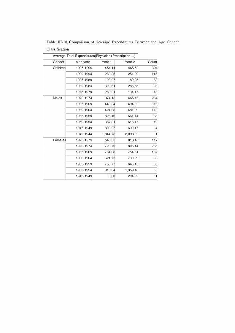
8/8/2019 Bulent Eris Model Development for Planning and Forecasting in Diagnostic and Treatment Systems 9022004
http://slidepdf.com/reader/full/bulent-eris-model-development-for-planning-and-forecasting-in-diagnostic-and 60/182
Table III-18 Comparison of Average Expenditures Between the Age Gender
ClassificationAverage Total Expenditures(Physician+Prescription ...)Gender birth year Year 1 Year 2 CountChildren 1995-1999 454.11 465.52 304
1990-1994 280.25 251.29 1461985-1989 198.97 189.25 681980-1984 302.61 286.55 281975-1979 269.21 134.17 13
Males 1970-1974 374.13 465.16 2641965-1969 448.34 494.92 3161960-1964 424.63 481.09 113
1955-1959 826.46 661.44 381950-1954 387.31 616.47 191945-1949 898.27 690.17 41940-1944 1,844.78 2,098.02 1
Females 1975-1979 548.00 818.45 1171970-1974 723.70 805.14 2651965-1969 784.03 754.61 1671960-1964 621.75 799.29 621955-1959 766.77 643.15 301950-1954 915.34 1,359.18 6
1945-1949 0.00 204.82 1

8/8/2019 Bulent Eris Model Development for Planning and Forecasting in Diagnostic and Treatment Systems 9022004
http://slidepdf.com/reader/full/bulent-eris-model-development-for-planning-and-forecasting-in-diagnostic-and 61/182

8/8/2019 Bulent Eris Model Development for Planning and Forecasting in Diagnostic and Treatment Systems 9022004
http://slidepdf.com/reader/full/bulent-eris-model-development-for-planning-and-forecasting-in-diagnostic-and 62/182
III.3 MOMENTS OF USAGE
First and second moments of the distributions are two basic estimators of the stochastic
nature of the distributions. As the distributions characteristics are changing with the age andgender, the data is analyzed according to 5 year age bands. While combining the different
weights of age and gender groups it is possible to derive the representative characteristics of
the whole group with the use of first and second moments.

8/8/2019 Bulent Eris Model Development for Planning and Forecasting in Diagnostic and Treatment Systems 9022004
http://slidepdf.com/reader/full/bulent-eris-model-development-for-planning-and-forecasting-in-diagnostic-and 63/182

8/8/2019 Bulent Eris Model Development for Planning and Forecasting in Diagnostic and Treatment Systems 9022004
http://slidepdf.com/reader/full/bulent-eris-model-development-for-planning-and-forecasting-in-diagnostic-and 64/182
Table III-21 Moments of Prescribed Drugs
Age AVG Pc N AVERAGE
n SECOND
MOMENT X AVERAGE
X SECOND
MOMENT %0-4 0.86 6.67 73.05 18.19 661.39 0.08
5-9 0.73 4.58 34.37 20.69 855.89 0.07
10-14 0.64 2.94 14.17 21.81 951.66 0.0515-19 0.58 2.97 14.44 21.41 917.07 0.03
20-24 0.55 2.82 13.06 23.99 1150.58 0.01
Male
16-20 0.58 2.51 11.41 22.00 975.00 0.0021-25 0.55 3.04 16.70 22.00 975.00 0.04
26-30 0.60 3.26 19.22 22.00 975.00 0.12
31-35 0.63 3.61 23.53 22.00 975.00 0.10
36-40 0.63 3.96 28.33 22.00 975.00 0.07
41-45 0.63 4.44 35.62 22.00 975.00 0.04
46-50 0.63 4.87 42.91 22.00 975.00 0.0351-55 0.67 5.71 59.06 22.00 975.00 0.01
56-60 0.70 6.83 84.34 22.00 975.00 0.0161-65 0.75 7.59 104.17 23.00 1030.02 0.00
66-70 0.75 8.35 126.10 23.00 1030.02 0.00
71-75 0.75 8.35 126.10 23.00 1030.02 0.00
Female
16-20 0.73 2.67 12.89 22.00 975.00 0.01
21-25 0.73 4.26 32.83 22.00 975.00 0.0626-30 0.75 4.39 34.85 22.00 975.00 0.10
31-35 0.75 4.56 37.66 22.00 975.00 0.0736-40 0.76 4.66 39.34 22.00 975.00 0.05
41-45 0.76 4.74 40.63 22.00 975.00 0.03
46-50 0.76 5.72 59.26 22.00 975.00 0.01
51-55 0.76 6.71 81.40 22.00 975.00 0.01
56-60 0.76 6.71 81.40 22.00 975.00 0.00
61-65 0.76 7.63 105.36 23.00 1030.02 0.00
66-70 0.76 8.55 132.41 23.00 1030.02 0.00
71-75 0.76 10.40 195.77 23.00 1030.02 0.00

8/8/2019 Bulent Eris Model Development for Planning and Forecasting in Diagnostic and Treatment Systems 9022004
http://slidepdf.com/reader/full/bulent-eris-model-development-for-planning-and-forecasting-in-diagnostic-and 65/182
Table III-22 Moments of Diagnostics
Age AVG Pc
n
AVERAGE
n SECOND
MOMENT X AVERAGE
X SECOND
MOMENT %0-4 0.52 2.7 24.63 35.62 2804.19 0.08
5-9 0.45 2.6 24.63 36.45 2935.61 0.07
10-14 0.35 1.89 14.98 42.05 3908.57 0.05
15-19 0.33 1.89 16.16 52.93 6192.49 0.03
20-24 0.34 2.11 19.95 73.33 11884.73 0.01Male
16-20 0.26 1.84 15.31 44.53 4382.26 0.00
21-25 0.34 2.04 18.66 53.75 6384.00 0.04
26-30 0.36 2.2 21.86 55.76 6871.54 0.12
31-35 0.38 2.35 24.8 62.78 8708.99 0.10
36-40 0.41 2.4 25.83 71.3 11235.6 0.07
41-45 0.43 2.49 27.93 76.73 13011.55 0.04
46-50 0.43 2.78 34.75 86.62 16583.16 0.03
51-55 0.45 3.11 43.65 86.62 16583.16 0.01
56-60 0.46 3.23 47.07 93.83 19455.78 0.01
61-65 0.46 3.35 50.62 101.03 22557.74 0.00
66-70 0.53 3.35 50.62 108.6 26064.13 0.00
71-75 0.7 3.35 50.62 112.53 27983.49 0.00
Female
16-20 0.44 2.2 21.84 53.87 6413.14 0.01
21-25 0.53 2.47 27.38 53.59 6347.97 0.06
26-30 0.53 2.66 31.8 57.23 7238.90 0.10
31-35 0.55 2.75 34.13 60.96 8212.72 0.07
36-40 0.55 2.99 40.33 66.11 9659.99 0.05
41-45 0.54 3.07 42.29 74.14 12149.00 0.03
46-50 0.56 3.4 52.04 78.73 13697.77 0.01
51-55 0.61 3.59 58.07 80.55 14339.27 0.01
56-60 0.55 4.17 78.14 88.06 17139.23 0.00
61-65 0.62 4.17 78.14 90.51 18104.63 0.00
66-70 0.56 4.17 78.14 96.63 20633.86 0.00
71-75 1 4.17 78.14 101.52 22776.26 0.00

8/8/2019 Bulent Eris Model Development for Planning and Forecasting in Diagnostic and Treatment Systems 9022004
http://slidepdf.com/reader/full/bulent-eris-model-development-for-planning-and-forecasting-in-diagnostic-and 66/182
Table III-23 Moments of Minor Treatment
Age AVG Pcn
AVERAGEn SECONDMOMENT X AVERAGE
X SECONDMOMENT %
0-4 0.21 2.56 13.10 14.97 1,120 0.085-9 0.14 2.14 9.19 21.25 2,257 0.07
10-14 0.11 1.88 7.09 28.71 4,122 0.05
15-19 0.12 2.11 8.91 36.82 6,778 0.03
20-24 0.10 2.49 12.41 61.68 19,021 0.01Male
16-20 0.10 1.72 5.92 42.59 9,071 0.00
21-25 0.09 1.95 8.83 49.36 12,184 0.04
26-30 0.11 1.95 8.83 51.82 13,426 0.12
31-35 0.13 1.95 8.83 5.82 13,426 0.10
36-40 0.12 1.95 8.83 57.83 16,723 0.07
41-45 0.13 1.95 8.83 62.44 19,495 0.0446-50 0.13 2.01 8.83 77.64 30,141 0.0351-55 0.13 2.01 8.83 83.25 34,652 0.0156-60 0.13 2.21 9.75 89.74 40,270 0.01
61-65 0.13 2.21 9.75 89.74 40,270 0.00
66-70 0.13 2.21 9.75 89.74 40,270 0.00
71-75 0.13 2.21 9.75 89.74 40,270 0.00
Female
16-20 0.11 1.86 6.90 43.43 9,431 0.01
21-25 0.14 2.01 8.10 47.08 11,084 0.0626-30 0.18 2.12 9.01 54.54 14,872 0.10
31-35 0.19 2.12 9.01 56.87 16,173 0.07
36-40 0.17 2.12 9.01 59.50 17,702 0.0541-45 0.17 2.12 9.01 66.40 22,042 0.03
46-50 0.17 2.12 9.01 73.60 27,082 0.01
51-55 0.17 2.51 12.57 113.30 64,188 0.01
56-60 0.17 2.51 12.57 162.18 131,519 0.00
61-65 0.17 2.51 12.57 162.18 131,519 0.0066-70 0.17 2.51 12.57 162.18 131,519 0.00
71-75 0.17 2.51 12.57 162.18 131,519 0.00
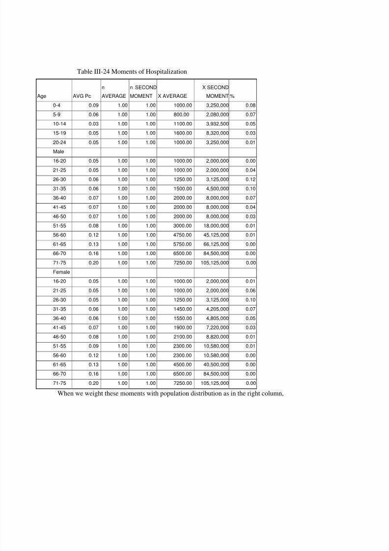
8/8/2019 Bulent Eris Model Development for Planning and Forecasting in Diagnostic and Treatment Systems 9022004
http://slidepdf.com/reader/full/bulent-eris-model-development-for-planning-and-forecasting-in-diagnostic-and 67/182
Table III-24 Moments of Hospitalization
Age AVG Pc
n
AVERAGE
n SECOND
MOMENT X AVERAGE
X SECOND
MOMENT %0-4 0.09 1.00 1.00 1000.00 3,250,000 0.08
5-9 0.06 1.00 1.00 800.00 2,080,000 0.07
10-14 0.03 1.00 1.00 1100.00 3,932,500 0.05
15-19 0.05 1.00 1.00 1600.00 8,320,000 0.03
20-24 0.05 1.00 1.00 1000.00 3,250,000 0.01Male
16-20 0.05 1.00 1.00 1000.00 2,000,000 0.00
21-25 0.05 1.00 1.00 1000.00 2,000,000 0.04
26-30 0.06 1.00 1.00 1250.00 3,125,000 0.12
31-35 0.06 1.00 1.00 1500.00 4,500,000 0.10
36-40 0.07 1.00 1.00 2000.00 8,000,000 0.07
41-45 0.07 1.00 1.00 2000.00 8,000,000 0.04
46-50 0.07 1.00 1.00 2000.00 8,000,000 0.03
51-55 0.08 1.00 1.00 3000.00 18,000,000 0.01
56-60 0.12 1.00 1.00 4750.00 45,125,000 0.01
61-65 0.13 1.00 1.00 5750.00 66,125,000 0.0066-70 0.16 1.00 1.00 6500.00 84,500,000 0.00
71-75 0.20 1.00 1.00 7250.00 105,125,000 0.00
Female16-20 0.05 1.00 1.00 1000.00 2,000,000 0.01
21-25 0.05 1.00 1.00 1000.00 2,000,000 0.0626-30 0.05 1.00 1.00 1250.00 3,125,000 0.10
31-35 0.06 1.00 1.00 1450.00 4,205,000 0.07
36-40 0.06 1.00 1.00 1550.00 4,805,000 0.0541-45 0.07 1.00 1.00 1900.00 7,220,000 0.03
46-50 0.08 1.00 1.00 2100.00 8,820,000 0.01
51-55 0.09 1.00 1.00 2300.00 10,580,000 0.01
56-60 0.12 1.00 1.00 2300.00 10,580,000 0.0061-65 0.13 1.00 1.00 4500.00 40,500,000 0.00
66-70 0.16 1.00 1.00 6500.00 84,500,000 0.00
71-75 0.20 1.00 1.00 7250.00 105,125,000 0.00
When we weight these moments with population distribution as in the right column,
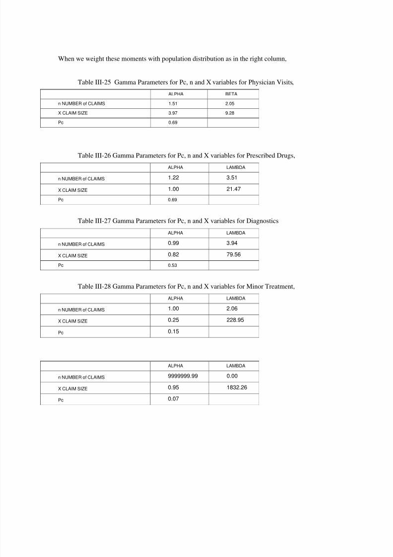
8/8/2019 Bulent Eris Model Development for Planning and Forecasting in Diagnostic and Treatment Systems 9022004
http://slidepdf.com/reader/full/bulent-eris-model-development-for-planning-and-forecasting-in-diagnostic-and 68/182
When we weight these moments with population distribution as in the right column,
Table III-25 Gamma Parameters for Pc, n and X variables for Physician Visits,ALPHA BETA
n NUMBER of CLAIMS 1.51 2.05
X CLAIM SIZE 3.97 9.28
Pc 0.69
Table III-26 Gamma Parameters for Pc, n and X variables for Prescribed Drugs,ALPHA LAMBDA
n NUMBER of CLAIMS 1.22 3.51
X CLAIM SIZE 1.00 21.47
Pc 0.69
Table III-27 Gamma Parameters for Pc, n and X variables for DiagnosticsALPHA LAMBDA
n NUMBER of CLAIMS 0.99 3.94
X CLAIM SIZE 0.82 79.56
Pc 0.53
Table III-28 Gamma Parameters for Pc, n and X variables for Minor Treatment,ALPHA LAMBDA
n NUMBER of CLAIMS 1.00 2.06
X CLAIM SIZE 0.25 228.95
Pc 0.15
ALPHA LAMBDA
n NUMBER of CLAIMS 9999999.99 0.00
X CLAIM SIZE 0.95 1832.26Pc 0.07

8/8/2019 Bulent Eris Model Development for Planning and Forecasting in Diagnostic and Treatment Systems 9022004
http://slidepdf.com/reader/full/bulent-eris-model-development-for-planning-and-forecasting-in-diagnostic-and 69/182
III.3.1 Comparison of the Data from Other Sources
When we compare our output with the Turkish and USA statistics, we see that mainindicators are close to the data that is gathered from private insurance for example ;
The National Ambulatory Medical Care Survey (NAMCS) is a national survey designed
to meet the need for objective, reliable information about the provision and use of ambulatory
medical care services in the United States. Also Health, United States, 2000 This report was
compiled by the Centers for Disease Control and Prevention (CDC), National Center for
Health Statistics (NCHS).
And also “Health Service Utilization Survey in Turkey” Ministry of Health, Turkey is a
very big sampled from overall Turkey with different income and educational levels [21]
Table III-29 Annual Number Physician Contacts
Age Group Private Insurance
Data
USA NAMCS data Health Service
Utilization Survey
in Turkey
0-14 M/F 3.11 2.95 1.84
15-44 Male 1.56 1.75 1.54
15-44 Female 2.54 3.25 2.74
45-64 Male 1.83 3.2 3.09
45-64 Female 2.83 4.2 4.48
Note: In private health insurance, maternity visits, optician controls are not included.

8/8/2019 Bulent Eris Model Development for Planning and Forecasting in Diagnostic and Treatment Systems 9022004
http://slidepdf.com/reader/full/bulent-eris-model-development-for-planning-and-forecasting-in-diagnostic-and 70/182
Table III-30 Annual Number Hospitalizations
Age GroupPrivate Insurance
Data
Health, United
States, 2000
Health Service
Utilization Survey
in Turkey
0-14 M/F 0.06 0.04 0.013-0.03
15-44 Male 0.06 0.085 (F/M) 0.025
15-44 Female 0.06 0.085(F/M) 0.059
45-64 Male 0.08 0.094-0.145(F/M) 0.061
45-64 Female 0.09 0.094-0.145(F/M) 0.072
In Health Service Utilization Survey in Turkey, to show the effect of various socio-
economic factors.
One of them is the Table V.19, this table conflicts the thesis(although it was mentioned
in the report) that increase in income level will increase the number of physician contacts
Table III-31 Physician contacts with different level of income
Physician contacts at age 15-44 band
Income level 1 1.66Income level 2 1.35
Income level 3 3.51
Income level 4 2.68
Income level 5 2.81

8/8/2019 Bulent Eris Model Development for Planning and Forecasting in Diagnostic and Treatment Systems 9022004
http://slidepdf.com/reader/full/bulent-eris-model-development-for-planning-and-forecasting-in-diagnostic-and 71/182
PART.IV.
THE MODEL
IV.1 ALTERNATIVE MODELS
There are various analytical or non analytic approaches to the aggregate distributions
(also called compound distributions). Especially in insurance the actuarial science is dealing
with the analytical solutions of the aggregate distributions.
The main course that we will benefit from actuarial literature are "Aggregate Loss
Models" Where sometimes referred as Compound Distributions.
There are alternative approaches to the problem which are; Moment based Approach(approximation), Recursive Algorithm, Inversion Methods, and simulation are used. No
method is clearly superior to other for all problems. Each method has both advantages and
disadvantages when compared with others.
IV.1.1 Moments Based Approach
In moment-based approach, moments of the aggregate distribution are calculated withthe moments of the compounding distributions. If the model can be based on a very familiar
distributions and the aggregate distribution is calculated to have a reasonable skew ness than
this method is the easiest way to calculate the models.

8/8/2019 Bulent Eris Model Development for Planning and Forecasting in Diagnostic and Treatment Systems 9022004
http://slidepdf.com/reader/full/bulent-eris-model-development-for-planning-and-forecasting-in-diagnostic-and 72/182

8/8/2019 Bulent Eris Model Development for Planning and Forecasting in Diagnostic and Treatment Systems 9022004
http://slidepdf.com/reader/full/bulent-eris-model-development-for-planning-and-forecasting-in-diagnostic-and 73/182
During the 10 years of experience a moment based model was build for calculating the
group proposals. The reason why a moment based model developed was it is the simplest and
fastest approach for forecasting health insurance quotations trough marketing people
In the model for aggregate distribution and limits various solutions were produced
sizenumber sizenumber annual avgavg 2222 .. σ σ σ += Equation IV-4
Having used the formulas above, related with the group being new or old,
different distributions may be found. These are
groupnumber groupsizegroupannual avgavgavg ___ .= Equation IV-5
If it is a new group, using variances and means of the size claim and number
distributions of the portfolio, a new annual distribution may be found.
portf number portf size portf annual avgavgavg ___ .= Equation IV-6
If we have the prior years experience for the group, , using variances and means of size
claim and number distributions formed with respect to the experience data, a new annual
distribution may be found.
).().( _2
_2
_2
__2
portf size portf number portf size portf number portf annual avgavg σ σ σ += Equation IV-7
If we have the prior years experience for the group,
The mean of size claim distribution via experience and the mean of size claim
distribution of the portfolio combined with a pre-defined coefficient Zi, portf+group sizeclaim average is found.
portf sizeigroupsizegroup portf size avg Z avg Z avg ____ ).1(. −+= Equation IV-8
The variance of size claim distribution via experience and the variance of size claim
distribution of the portfolio combined with a pre-defined coefficient Zq, portf+group size
claim variance is found.
groupsizegroupnumber groupsizegroupnumber groupannual avgavg _2
_2
_2
__2 .. σ σ σ += Equation IV-9
As a result of , setting this data into the formulas given above, variance and mean of
the annual distribution is found.
group portf number group portf sizegroup portf annual avgavgavg ______ .= Equation IV-10

8/8/2019 Bulent Eris Model Development for Planning and Forecasting in Diagnostic and Treatment Systems 9022004
http://slidepdf.com/reader/full/bulent-eris-model-development-for-planning-and-forecasting-in-diagnostic-and 74/182
IV.1.2 Recursive Algorithm
This method assumes a discrete claim severity distribution. By choosing a large enough
number of points for the claim severity distribution, one can obtain any desired degree of accuracy. For this reason, it has been called an “exact” method. This method requires far less
computer time than Monte Carlo simulation. Much of the mathematics involved is similar to
that used in the characteristic function in-version method. There are derivation of the
recursive method which does not involve inverting the Laplace transform designed in to work
for (a,b,0) and (a,b,1) parameter distributions pk = ( a + b/k) pk-1 [20]
IV.1.3 Inversion -Methods Fast Fourier-
By using canned routines which are available with many software packages using
vectors in complex number forms Discrete Fourier Transform - Fast Fourier Transform
method; Used both in convoluting and combining various distributions (physician visits and
prescribed drugs etc)
Direct Numerical Inversion; the method inverts the characteristic function of the
aggregate loss distribution using approximations like replacing severity distribution function
by piecewise linear distribution.
Here we define the Fourier application
Fast Fourier Transformation can be used to both combine n fold convolution
and also correlated benefits (physician + prescribed drugs) like simulation contrary to
moments based approach and recursive algorithm,
S x N n X xn
n( ) ( ) ( )*= ×
=
∞
∑0
Equation (IV-11)
))(()( )*1(* x X X x X nn∗= − Equation IV-12

8/8/2019 Bulent Eris Model Development for Planning and Forecasting in Diagnostic and Treatment Systems 9022004
http://slidepdf.com/reader/full/bulent-eris-model-development-for-planning-and-forecasting-in-diagnostic-and 75/182
Fourier Estimation
0
0,02
0,04
0,06
0,08
1 4 7 1 0
1 3
1 6
1 9
2 2
2 5
2 8
3 1
Fourier Es timation Real
Figure IV.1 Output for Prescribed Drugs of a Group
In this model an excel plus visual basic applications are used the model is
Two files of FFTsHT.xls and inputfile.xls is used
The input file has the n, X, and annual total variables and the macro creates the total
annual cost distribution by combining n and X distributions
This example was the combination of n and X, while combining two different benefits
again Fourier transformation can be used. In this case the formula will be [34]
( ) ( ) ( ) ( )[ ] ( )[ ]−−+= ∑ ji
j X i X jik X X k X X t t t t t t jik k
p
φ φ ω φ φ φ 111...,..., ,11,..., 11Equation (IV-13)
1 X φ are characteristic functions of the input distributions
ω is the correlation matrix for two different benefits
However the as the mathematics is complex for both explaining the problems in model
development (like below) simulation is preferred for development of the model

8/8/2019 Bulent Eris Model Development for Planning and Forecasting in Diagnostic and Treatment Systems 9022004
http://slidepdf.com/reader/full/bulent-eris-model-development-for-planning-and-forecasting-in-diagnostic-and 76/182
Figure IV.2 Second Fourier Example
IV.2 SIMULATION MODEL STRUCTUREModel that is provided here is made up of various parameters and variables, the simplest
technique was chosen. The structure is based on simulation and mathematical statistics, and
actuarial science is used.
@RISK is an Excel add-in software product that provides Excel to perform risk analysis
using Monte Carlo simulation in a spreadsheet based environment. @RISK Version 4.0.5.
Professional Edition of Palisade Corporation (where Best-fit software is also provided) is used
The model is formed of below 3 major modules where each module have different
subdivisions.
A. Individual Expenses Module
B. Experience and Credibility module
C. Group(Individual to Group) Module

8/8/2019 Bulent Eris Model Development for Planning and Forecasting in Diagnostic and Treatment Systems 9022004
http://slidepdf.com/reader/full/bulent-eris-model-development-for-planning-and-forecasting-in-diagnostic-and 77/182
IV.2.1 Individual Expenses Module
In this module with limits, deductibles and raw figures health care
expenditures/utilizations of one person for one year and shorter time periods are calculated,
All of these 3 variables are assumed to be have probability distributions and the
characteristics of these distributions are derived by
• Age
• GenderComment [B1]: AlthouStatus of health and Socioeconomic / geographic coare affecting the number aaverage cost of healthexpenditures, for each of tcategories of these differebands
Socio economic and geoconditions

8/8/2019 Bulent Eris Model Development for Planning and Forecasting in Diagnostic and Treatment Systems 9022004
http://slidepdf.com/reader/full/bulent-eris-model-development-for-planning-and-forecasting-in-diagnostic-and 78/182
START
INPUT NUMBER OF MEMBERS
ACCORDING TO AGE AND SEXDISTRIBUTION
Calculate the representative First and Second Moments forPc, n ,X
forPhysician, Prescription, Diagnostics,Minor Treatment and Hospitalization
from Age and Sex Bands
Calculate theParameters of the Distributions from the First and SecondMoments forPc (Binomial Dist.)n, X (Gamma Dist.)
forPhysician, Prescription, Diagnostics,Minor Treatment and Hospitalization
IF THE MODEL ISEXPERIENCE RATED
COMBINE THE CALCULATED Pc, nAND X PARAMETERS WITH PRIOR
GROUP DATA
Y
SIMULATIONITERATIONS
N
PERSON TOGROUP MODEL
Figure IV.3 Creation of the Input Parameters for Individual to Group Module +
Experience-Credibility Module

8/8/2019 Bulent Eris Model Development for Planning and Forecasting in Diagnostic and Treatment Systems 9022004
http://slidepdf.com/reader/full/bulent-eris-model-development-for-planning-and-forecasting-in-diagnostic-and 79/182
Simualtion Iterations
START
Loop up to Last Iterationand FINISH
Settingn via Gamma Dist.
SettingX's via Gamma Dist.
SettingPc via Binom Dist.
Settingmonth for each X viaEmpiricalDist.
Calculation of totalexpenditure and counts w.r.t.month
Generate Seed forPc, n ,X 's and month' s
forPhysician, Prescription,
Diagnostics,Minor Treatmentand Hospitalization
with the Spearman RankCorrelation forPc and n
Filter n and X's according to limits anddeductibles
Calculation ofAnnual Totals forCosts Incurred
Filtered with Limits and Deductibles
Combine Annual Totals forCosts Incurred
Filtered with Limits and Deductiblesmonthly expenditure and counts
in total sheet
Figure IV.4 Iteration of the Individual Expense Module(fed with credibility if any)

8/8/2019 Bulent Eris Model Development for Planning and Forecasting in Diagnostic and Treatment Systems 9022004
http://slidepdf.com/reader/full/bulent-eris-model-development-for-planning-and-forecasting-in-diagnostic-and 80/182
IV.2.1.1 Pc, n, X
These one-year expenditures can be formed of
• Medical Visit
• Drug• Diagnosis
• Minor Medical Treatment
• In-patient Treatment (Hospitalization)
The variables that are used in each category areo Pc (probability of claiming)o n (The frequency of treatment)
o X (Unit cost per treatment (i.e. one physician visit cost , cost of the drugs in oneprescription, one inpatient hospital stay )
IV.2.1.2 Age and Gender
For each 5 benefits there are 3 main category. Children, males and females have in total
29 different categories. Especially most of the health insurance models are calculating the
children in one category but statistics show us that different bands in children have 4 to 5
times different frequency figures and the groups can be very different children demographics
as well as adult demographics.
For different age and gender profiles of groups number of people in that age band are
used as weight factors to get the representative figures.
IV.2.1.3 Distribution Assumptions
For Pc, n and X which means total group of 435 converted to 15 (5 benefits * 3
‘Pc,n,X’). In such kind of a conversion, calculating different types of distributions for each
sub category is impossible. For Pc, Binomial distributions is used as Pc probabilities are not
very low(some times %90) Gamma is used for X and n distribution as it is a very flexibledistribution. After examining the distributions it was seen that Gamma was sufficient for most
of tail lengths(in the individual to group module large medical expenditures are inserted )and
being much more flexible, it was found suitable. For n as its out put is discrete a rounding is
done after the seed is executed and n is produced .

8/8/2019 Bulent Eris Model Development for Planning and Forecasting in Diagnostic and Treatment Systems 9022004
http://slidepdf.com/reader/full/bulent-eris-model-development-for-planning-and-forecasting-in-diagnostic-and 81/182
Here are the examples of the different shaped distributions considering the limits
0.00
0.05
0.10
0.15
0.20
0.25
0.30
1 6 1 1
1 6
2 1
2 6
3 1
risk GammaOutput
real hospitalclaims
Figure IV.5 Hospital Claim Cost X graph produced with gamma and real data
00.050.1
0.150.2
0.250.3
1 4 7 1 0
1 3
1 6
1 9
# DR Real
# DRGammaRisk
Figure IV.6 Number of Physician Visits n graph produced with gamma and real
data
According to Gamma Beta is Variance / Average and Alpha is Average / Beta
Comment [B2]: 3 no luçalışması
Comment [B3]: 3 noluolan d bank verilerini = daarındırıp çalıştık

8/8/2019 Bulent Eris Model Development for Planning and Forecasting in Diagnostic and Treatment Systems 9022004
http://slidepdf.com/reader/full/bulent-eris-model-development-for-planning-and-forecasting-in-diagnostic-and 82/182
IV.2.1.4 Limits and Deductibles
In various social security and private health systems, limits and deductibles are applied.
The effect of these may be very interesting to the aggregate cost or total utilization.
In private insurance systems and some times social security benefits are limited or
applied deductibles.
Briefly Deductible is “Amount of expenses that the insured party must pay before
receiving any benefits from the insurance company” and limit is “the maximum dollar amount
that an insurance company will pay based on annual total or case, illness definition”[14]
Limits are the maximum amounts that the risk career (private or social security fund)
will not compensate above. Deductibles are the minimum amounts that the risk career will not
compensate below.
In the model following types of limits and deductibles can be applied.
• Annual number of case unit (Maximum/out of pocket Number of expenditures
for 1 year applied ton),limit / deductible
• Per case limit /deductible(Cost of each expenditure applied toX)
• Annual USD limit/deductible (Maximum amount of expenditure in USD terms
for 1 year)
Deductibles with the limit category are defined.

8/8/2019 Bulent Eris Model Development for Planning and Forecasting in Diagnostic and Treatment Systems 9022004
http://slidepdf.com/reader/full/bulent-eris-model-development-for-planning-and-forecasting-in-diagnostic-and 83/182
Figure IV.7 Limit and Deductible Application Process
Limits and deductibles are drastically affecting the overall characteristics of the costs
and utilizations as well as total and benefit basis. When we compare the limited number of
utilizations and total cost with health care spending without limit and the total cost of the
expenditures after the limits, the shape of the distribution is changing.

8/8/2019 Bulent Eris Model Development for Planning and Forecasting in Diagnostic and Treatment Systems 9022004
http://slidepdf.com/reader/full/bulent-eris-model-development-for-planning-and-forecasting-in-diagnostic-and 84/182
0
5 0
1 0 0
1 5 0
2 0 0
Costs Occurred0
0.10.20.30.40.50.6
0.70.8
Costs Occurred 0.554 0.06 0.039 0.035 0.028 0.025 0.026 0.021 0.021 0.019
Annual Limits of 150$ 0.554 0.06 0.039 0.035 0.028 0.025 0.259 0 0 0
Annual Limits of 150$+ AnnualDeductible of 50$ 0.653 0.035 0.028 0.025 0.259 0 0 0 0 0
Annual Limits of 2000$ 0.554 0.06 0.039 0.035 0.028 0.025 0.026 0.021 0.021 0.019
Annual Limits o f 2000$+Annual Deduct ible of 100$
0.716 0.025 0.026 0.021 0.021 0.019 0.015 0.016 0.013 0.012
0 25 50 75 100 125 150 175 200 225
Figure IV.8 Limit and Deductible Affect On Diagnostic Annual Costs
Similar affects occur for the total of the costs from various benefits and deductibles

8/8/2019 Bulent Eris Model Development for Planning and Forecasting in Diagnostic and Treatment Systems 9022004
http://slidepdf.com/reader/full/bulent-eris-model-development-for-planning-and-forecasting-in-diagnostic-and 85/182
1 4 7 1 0
1 3
1
6
1 9
CLAIMSINCURRED
00.10.20.30.40.50.60.70.80.9
CLAIMS INCURRED 0.048 0.509 0.211 0.086 0.049 0.036 0.016 0.012 0.007 0.005 0.004 0.004 0.003 0.002 0.003 0 0 9E-04 0 0 0
NUMBER OF CLAIMS0 .048 0 .036 0 .044 0 .063 0 .044 0 .057 0 .068 0 .047 0 .057 0 .043 0 .045 0 .043 0 .049 0 .032 0 .036 0 .029 0 .03 0 .03 0 .019 0 .019 0 .308
HYBRID LIMITED1 0.03 0.627 0.229 0.031 0.02 0.016 0.016 0.017 0.012 0 0 0 0 0 0 0 0 0 0 0 0
HYBRID LIMITED2 0.036 0.842 0.046 0.019 0.019 0.01 0 .027 9E-04 0 0 0 0 0 0 0 0 0 0 0 0 0
HYBRID LIMITED3 0.03 0.45 0.27 0.117 0.047 0.025 0.016 0.015 0.005 0.004 0.004 0.005 0.002 0.002 0.003 0 0 0 0 0 9E-04
HYBRID LIMITED4 0.538 0 .379 0 .047 0.012 0.007 0 .003 0 .002 0 .003 0.004 9E-04 0 0 0 0 0 0 0.003 0 0 0 0
1 2 3 4 5 6 7 8 9 10 11 12 13 14 15 16 17 18 19 20 21
Figure IV.9 When various scenarios Applied Total Costs on Individual Basis
IV.2.1.5 Dependency
While producing the seed for the input of these 3 variables Pc and n distributions are
correlated with Spearman Rank Correlation. from the observation it was found that the annual
number of treatment and probability of claiming(Pc) is correlated with each other.
In the model distributions of Pc and n are correlated by @RISK with spearman
correlation where the input Coefficient are entered with matrixes. The rank-order correlationcoefficient was developed by C. Spearman in the early 1900's. It is calculated using rankings
of values, not actual values themselves (as is the linear correlation coefficient). A value's
"rank" is determined by its position within the min-max range of possible values for the
variable. The coefficient is a value between -1 and 1, which represents the desired degree of

8/8/2019 Bulent Eris Model Development for Planning and Forecasting in Diagnostic and Treatment Systems 9022004
http://slidepdf.com/reader/full/bulent-eris-model-development-for-planning-and-forecasting-in-diagnostic-and 86/182
correlation between the two variables during sampling. Positive coefficient values indicate a
positive relationship between the two variables — when the value sampled for one is high, the
value sampled for the second will also tend to be high. Negative coefficient values indicate an
inverse relationship between the two variables — when the value sampled for one is high, the
value sampled for the second will tend to be low. @RISK generates rank-correlated pairs of
sampled values in a two-step process. First, a set of randomly distributed "rank scores" are
generated for each variable. If 100 iterations are to be run, for example, 100 scores are
generated for each variable. (Rank scores are simply values of varying magnitude between a
minimum and maximum. @RISK uses Van der Waerden scores based on the inverse function
of the normal distribution). These rank scores are then rearranged to give pairs of scores,
which generate the desired rank correlation coefficient. For each iteration there is a pair of
scores, with one score for each variable.
Using the resources that are presented in the previous chapters as actuarial or other
predicting techniques, we try to take out the risk factors and identify the parameters of the
model affecting the health care demand. When we try to structure the predicting techniques
we have the parameters to be used in the model,
The spearman correlation coefficients for the Probability of claiming as follows;
Table IV-1 Spearman Rank Correlations For Ratio of User Input Data(Pc)
NewMatrixPc (5x5)dr!B8
binom Pc / ALPHA
pres!B8binom Pc /
ALPHA
diagnostic!B8binom Pc /
ALPHA
minortreat!B8binom Pc /
ALPHA
hospital!B8binom Pc /
ALPHAdr!B8
binom Pc / ALPHA1
pres!B8binom Pc / ALPHA
0.616 1
diagnostic!B8binom Pc / ALPHA
0.586 0.466 1
minortreat!B8binom Pc / ALPHA
0.273 0.324 0.286 1
hospital!B8binom Pc / ALPHA
0.596 0.396 0.485 0.423 1

8/8/2019 Bulent Eris Model Development for Planning and Forecasting in Diagnostic and Treatment Systems 9022004
http://slidepdf.com/reader/full/bulent-eris-model-development-for-planning-and-forecasting-in-diagnostic-and 87/182
Table IV-2 Spearman Rank Correlations For Number of Usage Input Data(n)
NewMatrixadet(5x5)
dr!B9n
PRODUCER / ALPHA
pres!B9n
PRODUCER / ALPHA
diagnostic!B9
n PRODUCER / ALPHA
minortreat!B9
n PRODUCER / ALPHA
hospital!B9
n PRODUCER / ALPHA
dr!B9n PRODUCER /
ALPHA1
pres!B9n PRODUCER /
ALPHA0.668 1
diagnostic!B9
n PRODUCER / ALPHA 0.57 0.4 1
minortreat!B9n PRODUCER /
ALPHA0.309 0.345 0.239 1
hospital!B9n PRODUCER /
ALPHA0.456 0.396 0.359 0.385 1
Uncertainty approach for the level of dependency problem can also be used if
appropriate software and configuration is handled. There is an example for the application of
Fourier transformation in the Appendix.
IV.2.1.6 Short Term Monthly Analysis
This question arises from the question if we have the stats of one-two month of a
population that we know census (like Turkey pop.) what kind of uncertainties exists and is itpossible to derive an estimation formula which has parameters of limits for expense issues,
deductibles, demographic etc, and other economic input.
This is possibly the most interesting issues complicating because of the shorter time
period creates a bigger randomness in nature. Study. In this part aggregate costs are calculated

8/8/2019 Bulent Eris Model Development for Planning and Forecasting in Diagnostic and Treatment Systems 9022004
http://slidepdf.com/reader/full/bulent-eris-model-development-for-planning-and-forecasting-in-diagnostic-and 88/182

8/8/2019 Bulent Eris Model Development for Planning and Forecasting in Diagnostic and Treatment Systems 9022004
http://slidepdf.com/reader/full/bulent-eris-model-development-for-planning-and-forecasting-in-diagnostic-and 89/182
Distribution of "n" in Monthly intervals
0
0.05
0.1
0.15
0.2
0.25
0.30.35
0.4
1 2 3 4 5 6 7 8 9 10 11
Real "n" in August Real "n" in March
Figure IV.11 Distribution of "n" in March and August
When we compare the real data for March And August, considering n, following results
occurred

8/8/2019 Bulent Eris Model Development for Planning and Forecasting in Diagnostic and Treatment Systems 9022004
http://slidepdf.com/reader/full/bulent-eris-model-development-for-planning-and-forecasting-in-diagnostic-and 90/182
Table IV-3 Descriptive Statistics of Monthly FiguresReal Costs
Occurred inMarch
Real CostsOccurred in
August
CLAIMSINCURRED in All
YearNo. of values used 1951 1951 1951No. of values ignored 0 0 0No. of min. val. 1602 1518 852% of min. val. 82.112 77.806 43.670Minimum 0.000 0.000 0.0001st quartile 0.000 0.000 0.000Median 0.000 0.000 46.2643rd quartile 0.000 0.000 274.225Maximum 1011.270 1875.490 7694.798Range 1011.270 1875.490 7694.798Sum 22097.932 27899.751 468342.505Mean 11.326 14.300 240.053Geometric meanHarmonic meanKurtosis 156.706 293.945 50.291Skewness 11.302 15.618 5.593Kurtosis 157.276 295.008 50.478Skewness 11.320 15.642 5.601CV (standard deviation/mean) 5.047 5.476 2.137Sample variance 3266.456 6128.155 263017.830Estimated variance 3268.131 6131.298 263152.711Sample standard deviation 57.153 78.283 512.853Estimated standard deviation 57.168 78.303 512.984Mean absolute deviation 18.868 22.777 284.704Median absolute deviation 0.000 0.000 46.264Standard-error 1.294 1.773 11.614Lower bound. Mean IC 8.788 10.824 217.276Upper bound. Mean IC 13.865 17.777 262.829
When we examine these results we can say that Coefficient of Variation increase in
monthly statistics(as would be expected)
Comparing the monthly costs occurred between August and March
Note: The calculation of the Mann-Whitney's U takes ties into account

8/8/2019 Bulent Eris Model Development for Planning and Forecasting in Diagnostic and Treatment Systems 9022004
http://slidepdf.com/reader/full/bulent-eris-model-development-for-planning-and-forecasting-in-diagnostic-and 91/182
Table IV-4 Mann-Whitney U test (two-tailed test) for Monthly Incurred CostsU 673737.000U (expected value) 715208.000U (variance) 185183031.030
Z (observed value) -3.048Z (critical value) 1.960Two-tailed p-value 0.002Alpha 0.050
The Mann-Whitney's U is normalized and tested against the normal distribution
Decision: At the level of significance alpha=0.050 the decision is to reject the null
hypothesis of absence of difference between samples. In other words, the difference between
samples is significant.
Kolmogorov-Smirnov test / two-tailed test:Table IV-5 Kolmogorov-Smirnov(two-tailed test) test for Monthly Incurred
CostsD 0.063Two-tailed p-value 0.017Alpha 0.050
Decision:
At the level of significance alpha=0.050 the decision is to reject the null hypothesis of
absence of difference between samples. In other words, the difference between samples is
significant.
Also when we do the comparison between number of expenditures
Note: The calculation of the Mann-Whitney's U takes ties into account
Table IV-6 Mann-Whitney's U (two-tailed test) test for Monthly Number of
UtilizationsU 673325.500
U (expected value) 715208.000U (variance) 184916515.611Z (observed value) -3.080Z (critical value) 1.960Two-tailed p-value 0.002Alpha 0.050

8/8/2019 Bulent Eris Model Development for Planning and Forecasting in Diagnostic and Treatment Systems 9022004
http://slidepdf.com/reader/full/bulent-eris-model-development-for-planning-and-forecasting-in-diagnostic-and 92/182
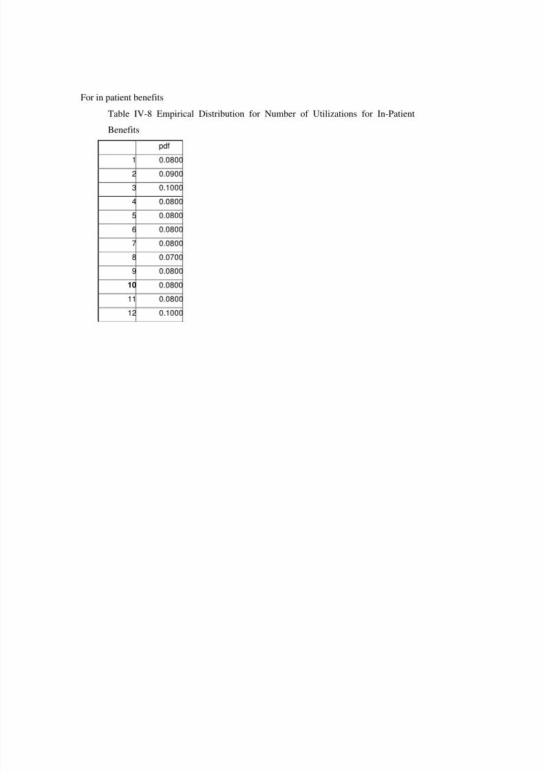
8/8/2019 Bulent Eris Model Development for Planning and Forecasting in Diagnostic and Treatment Systems 9022004
http://slidepdf.com/reader/full/bulent-eris-model-development-for-planning-and-forecasting-in-diagnostic-and 93/182
For in patient benefits
Table IV-8 Empirical Distribution for Number of Utilizations for In-Patient
Benefitspdf
1 0.08002 0.09003 0.10004 0.08005 0.08006 0.08007 0.08008 0.0700
9 0.080010 0.080011 0.080012 0.1000

8/8/2019 Bulent Eris Model Development for Planning and Forecasting in Diagnostic and Treatment Systems 9022004
http://slidepdf.com/reader/full/bulent-eris-model-development-for-planning-and-forecasting-in-diagnostic-and 94/182
All of these Number of cases and total expenditure are presented in each benefit sheet
and also are summed in a summary sheet, which creates one member’s outputMinimum 0
Mean 40.37111
Maximum 11928.55
Std Dev 229.8935
Variance 52851.01
Skewness 25.40516
Kurtosis 1010.965
Mode 0
Left X 0
Left P 5%
Right X 196.7438
Right P 95%Diff. X 196.7438
Diff. P 90%
5th Perc. 0
95th Perc. 196.7438
#Errors 0
Filter Min
Filter Max
#Filtered 0
IV.2.2 Experience - Credibility Module
Although we combine the sub groups according to age and gender and analyze the risk
in uniform sub groups in terms of medical expense and utilizations, we can always improve
our estimations with the experience of that group in the following periods. (we will be dealing
with prospective experience rating techniques as this study is focused on the prediction)
Credibility Theory is one of the most well examined subjects in actuarial profession
within the names of "credibility rating" and "experience rating" dealing with this and has been
published various articles on non-life insurance, disability and life.

8/8/2019 Bulent Eris Model Development for Planning and Forecasting in Diagnostic and Treatment Systems 9022004
http://slidepdf.com/reader/full/bulent-eris-model-development-for-planning-and-forecasting-in-diagnostic-and 95/182
Credibility is a procedure by which data external to a particular group or individual are
combined with the experience of the group or individual in order to better estimate te
expected loss(or any other statistical quantity) for each group or quantity.
The external data are typically a rate that has been determined based on historical data
from other, similar policies. The internal data are the experience of the individual or group
itself. Often the calculation is reduced to a very simple form [12].
PrRatedE.premiumportfolio*Z)-(1experiencegroup *Z =+ Equation (IV-14)
Z= credibility factor
Group experience
If the experience size of the group is enough we can base our calculation according to
experience of the group(with the inflationary assumptions etc.) however the question for what
is the group size that the experience should be based on 100% is usually unknown.
In the applications standard tables are used like this.[25, 26]
Table IV-9 Credibility ratings for groups with at least 3 year’s claims history
Number of Peaople Credibility Rates
50 to 99 35-50%
100 to 399 50-70%
400 to 999 70-90%
1000 or more 100%
However we structured the model based on much more sophisticated grounds.
Z is calculated for each benefit (for hospitalization, physician fees, prescribed drugs
etc.) as each of these benefits is defined separately for each group.
• The size of the group
• The limit amount of the benefit (large claims require more experience)
• The incidence rate of the claims

8/8/2019 Bulent Eris Model Development for Planning and Forecasting in Diagnostic and Treatment Systems 9022004
http://slidepdf.com/reader/full/bulent-eris-model-development-for-planning-and-forecasting-in-diagnostic-and 96/182
• The number of years experienced
Affects the Z. Z = sqrt of (n / n100%) [18]
n100% is the group size that gives us the full credibility for experience rating
2%100 )
*..*)((
eter RangeParamestimate AVGprior estimateSTDprior confidence NormInv
n = Equation (IV-15)
100%
.
nn
Z concerned groupsize partial =
Equation (IV-16)
concerned groupsize partial nconfidence NormInveter RangeParam
STD AVG
Z .)(×= Equation IV-17
According to this formula for 0,95 confidence and 0,1 accepted deviation, normal
inverse function output is 1.64(=NORMINV(0.95;0;1)) and
(Normal-Inverse / Range Parameter) =(1.65 / 0.1)=16.5
For each variable the Prior year averages and standard deviation will be calculated and
after that according to cases handled the “group size concerned” will be calculated.
We calculate the required number of experience cases for each variable of Pc, n, X to
get 100% credibility in the experience formula (Z to be taken 1 and (1-Z) to be 0).
In Pc as every insured will be a case experience for us for the probability of claiming,
we will be counting the member of the group to give the credibility

8/8/2019 Bulent Eris Model Development for Planning and Forecasting in Diagnostic and Treatment Systems 9022004
http://slidepdf.com/reader/full/bulent-eris-model-development-for-planning-and-forecasting-in-diagnostic-and 97/182
Pc AVG STD n100% Physician Visits 0.69 0.46 122
Prescribed Drugs 0.69 0.46 122
Diagnostic Procedures 0.53 0.49 240Minor Treatment 0.15 0.36 1533
Hospital Treatment 0.07 0.26 3595
For n the required number of cases is calculated byn100% but as the all the members are
not spending health care expenditures(Pc is always <1) we have to divide the result of the
n AVG STD Required number of
member (n100% / Pc)
Physician Visits 3.10 2.52 179 / 0.69=260
Prescribed Drugs 4.28 3.88 222/0.69=321
Diagnostic Procedures 3.9 3.92 273/0.53=516
Minor Treatment 1 2.26 271/0.15=1804
Hospital Treatment 1 1 3595
X AVG STD Required number of member (n100% / Pc Xn)
Physician Visits 36.84 18.49 68 / 0.69 X 3.1=32
Prescribed Drugs 21.47 21.47 271 / 0.69 X 4.28=92
Diagnostic Procedures 65.24 72.04 330 / 0.53 X3.9=160
Minor Treatment 57.24 114.48 1082 / 0.15 X
2.06=3502
Hospital Treatment 1740.65 1785.87 285 /0.07 X1 =4068
For each variable there are different credibility weights.

8/8/2019 Bulent Eris Model Development for Planning and Forecasting in Diagnostic and Treatment Systems 9022004
http://slidepdf.com/reader/full/bulent-eris-model-development-for-planning-and-forecasting-in-diagnostic-and 98/182

8/8/2019 Bulent Eris Model Development for Planning and Forecasting in Diagnostic and Treatment Systems 9022004
http://slidepdf.com/reader/full/bulent-eris-model-development-for-planning-and-forecasting-in-diagnostic-and 99/182

8/8/2019 Bulent Eris Model Development for Planning and Forecasting in Diagnostic and Treatment Systems 9022004
http://slidepdf.com/reader/full/bulent-eris-model-development-for-planning-and-forecasting-in-diagnostic-and 100/182

8/8/2019 Bulent Eris Model Development for Planning and Forecasting in Diagnostic and Treatment Systems 9022004
http://slidepdf.com/reader/full/bulent-eris-model-development-for-planning-and-forecasting-in-diagnostic-and 101/182
The Trend parameter allows for gradual movements of the inception and termination
rate parameters away from their starting points over time. The shock parameter allows for
sudden jumps in experience, for example due to a change in the legal environment
)}1).(1{(_
1k k k k
Module IndivGroupSize
i
DC B A EmpirDist ++++∑=
Equation IV-19
Individual to Group Formula with Uncertainty from Different Factors
Ak = representing credibility risk (iteration k)
Bk = representing appropriateness risk (iteration k)
Ck = representing trend risk (iteration k)
Dk = representing shock risk (iteration k)
For A, B and C normal distribution issuedParameter Avg StdCredibility 0% 20%Appropriateness 0% 20%Trend 1% 2.50%
Equation IV-20 Normal Distribution Parameters N(µ, σ)
For the Shock risk Generalized Distribution is usedx f(x)
-30 0-29 0.05-1 0.10 99.71 0.1
29 0.0530 0
Equation IV-21 Shock Risk Generalized Distribution Points

8/8/2019 Bulent Eris Model Development for Planning and Forecasting in Diagnostic and Treatment Systems 9022004
http://slidepdf.com/reader/full/bulent-eris-model-development-for-planning-and-forecasting-in-diagnostic-and 102/182
Simualtion Iterations for Individual to Group
START
Setting Individual Module OutputX's viaEmprical Dist.
Setting Uncertainty from credibility of thedata via Normal Dist.
Generate Seed for
Pc, n ,X 's and month' sforPhysician, Prescription,
Diagnostics,Minor Treatmentand Hospitalization
with the Spearman RankCorrelation forPc and n
Calculation ofAnnual Totals
Setting Uncertainty from suitability of thedata via Normal Dist.
Setting Uncertainty from allowance forshocks via Generalized Dist.
Setting Uncertainty from trends viaNormal Dist.
Figure IV.12 Flow Process for the Individual to Group Module
IV.2.4 Characteristics of the Model Output and SensitivityIn this section with the help of the model we examined the characteristics that we
cannot examine in real life like effect of dependency, group size(statistical fluctuation) and
Uncertainty due to factors mentioned in Individual to Group Module. After examining these
an overall sensitivity is done according to the parameters that has on effect on the costs and
limit/deductible is provided.

8/8/2019 Bulent Eris Model Development for Planning and Forecasting in Diagnostic and Treatment Systems 9022004
http://slidepdf.com/reader/full/bulent-eris-model-development-for-planning-and-forecasting-in-diagnostic-and 103/182
IV.2.4.1 The Effect of Dependency
Using the individual model and testing the sensitivity of the correlation matrix below
output is gathered.
If we take the Spearman correlations as 0 tha below results are taken
Table IV-10 Summary Statistic of the Total Costs Incurred(Independent of the
limits)
NameWith real
correlation
With allcorrelation input –
0.25
With allcorrelation input
0
With allcorrelation input
1
Minimum 0 0 0 0Mean 337.15 350.98 349.40 335.43Maximum 10,592.66 9,762.28 13,968.36 11,001.53Std Dev 657.61 562.09 620.02 547.87Variance 432,446.40 315,940.80 384,420.90 300,159.30Skewness 5.64 6.99 6.17 7.56Kurtosis 52.52 71.79 67.44 91.66Mode 0 0 0 0Left X 0 21.31772 0 0Left P 5% 5% 5% 5%
Right X 1289.10 905.06 1183.33 951.26Right P 95% 95% 95% 95%Diff. X 1289.10 883.74 1183.33 951.26

8/8/2019 Bulent Eris Model Development for Planning and Forecasting in Diagnostic and Treatment Systems 9022004
http://slidepdf.com/reader/full/bulent-eris-model-development-for-planning-and-forecasting-in-diagnostic-and 104/182
Table IV-11 Distribution of the Total Costs Incurred(Independent of the limits)
TOTAL COST0
CORREL'-
0.25CORREL1
CORRELREAL
CORRELGrand
Total0 6.77% 2.77% 34.18% 17.71% 15.36%1-500 75.87% 81.28% 45.81% 62.33% 66.32%501-1000 12.85% 11.75% 12.24% 13.18% 12.51%1001-1500 2.18% 1.69% 3.85% 3.52% 2.81%1501-2000 0.82% 0.65% 1.60% 1.18% 1.06%2001-2500 0.39% 0.49% 0.81% 0.63% 0.58%2501-3000 0.36% 0.32% 0.34% 0.33% 0.34%3001-3500 0.17% 0.29% 0.32% 0.29% 0.27%3501-4000 0.17% 0.20% 0.21% 0.27% 0.21%4001-4500 0.09% 0.20% 0.16% 0.12% 0.14%4501-5000 0.10% 0.06% 0.16% 0.09% 0.10%5001-5500 0.05% 0.11% 0.06% 0.18% 0.10%5501-6000 0.00% 0.01% 0.07% 0.05% 0.03%6001-6500 0.04% 0.04% 0.05% 0.03% 0.04%6501-7000 0.03% 0.04% 0.03% 0.00% 0.03%7001-7500 0.01% 0.02% 0.00% 0.02% 0.01%7501-8000 0.03% 0.03% 0.03% 0.02% 0.03%8001-8500 0.03% 0.01% 0.02% 0.02% 0.02%8501-9000 0.01% 0.03% 0.02% 0.01% 0.02%9001-9500 0.01% 0.00% 0.02% 0.00% 0.01%9501-10000 0.00% 0.01% 0.00% 0.01% 0.01%10001-10500 0.01% 0.00% 0.01% 0.00% 0.01%10501-11000 0.01% 0.00% 0.01% 0.00% 0.01%13501-14000 0.00% 0.00% 0.00% 0.01% 0.00%Grand Total 100.00% 100.00% 100.00% 100.00% 100.00%

8/8/2019 Bulent Eris Model Development for Planning and Forecasting in Diagnostic and Treatment Systems 9022004
http://slidepdf.com/reader/full/bulent-eris-model-development-for-planning-and-forecasting-in-diagnostic-and 105/182

8/8/2019 Bulent Eris Model Development for Planning and Forecasting in Diagnostic and Treatment Systems 9022004
http://slidepdf.com/reader/full/bulent-eris-model-development-for-planning-and-forecasting-in-diagnostic-and 106/182
IV.2.4.2 The Effect of Group Size and Uncertainty on Individual to Group
Module
By just iterating the model to examine the statistical fluctuation combining the twoprobabilities for 2 different groups where the first one has 50 members and the secondhas 500 the simulation of 10.000 iterations gives us the distribution of total cost perheadas follows;
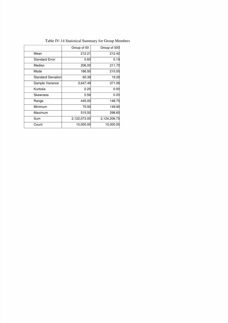
8/8/2019 Bulent Eris Model Development for Planning and Forecasting in Diagnostic and Treatment Systems 9022004
http://slidepdf.com/reader/full/bulent-eris-model-development-for-planning-and-forecasting-in-diagnostic-and 107/182

8/8/2019 Bulent Eris Model Development for Planning and Forecasting in Diagnostic and Treatment Systems 9022004
http://slidepdf.com/reader/full/bulent-eris-model-development-for-planning-and-forecasting-in-diagnostic-and 108/182
When we examine these out puts with the uncertainty modifications in Individual to
Group Module section
Table IV-15 Distribution Output for Group Members
50 withuncertainty
500 withuncertainty
50 nouncertainty
500 nouncertainty
500 noshockvariable
0 0.000 0.000 0.000 0.000 0.00025 0.000 0.000 0.000 0.000 0.00050 0.000 0.000 0.000 0.000 0.00075 0.000 0.000 0.000 0.000 0.000
100 0.007 0.000 0.004 0.000 0.000
125 0.039 0.000 0.046 0.000 0.000150 0.081 0.000 0.098 0.000 0.000175 0.107 0.002 0.145 0.017 0.019200 0.119 0.034 0.173 0.257 0.230225 0.114 0.154 0.154 0.484 0.454250 0.113 0.257 0.136 0.211 0.248275 0.093 0.222 0.093 0.031 0.047300 0.074 0.129 0.066 0.001 0.003325 0.058 0.068 0.039 0.000 0.000350 0.044 0.046 0.023 0.000 0.000375 0.036 0.034 0.013 0.000 0.000400 0.024 0.019 0.007 0.000 0.000425 0.017 0.014 0.002 0.000 0.000450 0.011 0.007 0.001 0.000 0.000475 0.009 0.005 0.001 0.000 0.000500 0.008 0.003 0.000 0.000 0.000

8/8/2019 Bulent Eris Model Development for Planning and Forecasting in Diagnostic and Treatment Systems 9022004
http://slidepdf.com/reader/full/bulent-eris-model-development-for-planning-and-forecasting-in-diagnostic-and 109/182
0
1000
2000
3000
4000
5000
6000
1 2 3 4 5 6 7 8 9 10 11 12 13 14 15 16 17 18 19 20 21 22 23
50 w ith uncertainty
500 w ith uncertainty
50 no uncertainty
500 no uncertainty
500 no shock variable
Equation IV-22 Average Expenditure Per Member For Groups with Different
Number of Members
IV.2.4.3 Sensitivity
In order to identify the most critical inputs in our model we make the sensitivity
analysis. In below graph These results show the sensitivity of each output variable to its inputvariables. The Sensitivity analysis performed on the output variables and their associated
inputs uses either a multivariate stepwise regression analysis or a rank order correlation
analysis. The input distributions in the model are ranked by their impact on the output. In the
@RISK software, multiple regression tries to fit multiple input data sets to a planar equation
that could produce the output data set. The sensitivity values returned by @RISK are
normalized variations of the regression coefficients. During this stepwise regression technique
is used as it is is preferable for large numbers of inputs since it removes all variables that
provide an insignificant contribution from the model. The second technique used is a rankcorrelation calculation. With this analysis, correlation coefficients are calculated between the
output values and each set of sampled input values. The results of each form of sensitivity
analysis are displayed as a "tornado" type chart, with longer bars at the top representing the
most significant input variables.

8/8/2019 Bulent Eris Model Development for Planning and Forecasting in Diagnostic and Treatment Systems 9022004
http://slidepdf.com/reader/full/bulent-eris-model-development-for-planning-and-forecasting-in-diagnostic-and 110/182
Regression Sensitivity for TOTAL COSTINCURRED / After P...
Std b Coefficients
TOTAL COST INCURRED/M11 .031
TOTAL COST INCURRED/N11 .031
TOTAL COST INCURRED/K11 .034
date/N9-.035
TOTAL COST INCURRED/Q11 .039
TOTAL COST INCURRED / LIMI.../D11 .047
date/P9 .061
bınom Pc / ALPHA/B8 .064
bınom Pc / ALPHA/B8 .065
bınom Pc / ALPHA/B8 .086
n PRODUCER / ALPHA/B9 .099
n PRODUCER / ALPHA/B9 .118
TOTAL COST INCURRED / LIMI.../D11 .126
bınom Pc / ALPHA/B8 .142
n PRODUCER / ALPHA/B9 .213
bınom Pc / ALPHA/B8 .549
-1 -0.75 -0.5 -0.25 0 0.25 0.5 0.75 1
Figure IV.13 Std B coefficients for Total Costs Incurred

8/8/2019 Bulent Eris Model Development for Planning and Forecasting in Diagnostic and Treatment Systems 9022004
http://slidepdf.com/reader/full/bulent-eris-model-development-for-planning-and-forecasting-in-diagnostic-and 111/182
Table IV-1612 Std B coefficients for Total Costs IncurredRank
for totalsheet!B11 Cell Name
B11 / TOTAL
COST INCURRED / After Pc % Regression
#1 hospital!B8 bınom Pc / ALPHA 0.549#2 diagnostic!B9 n PRODUCER / ALPHA 0.213#3 diagnostic!B8 bınom Pc / ALPHA 0.142#4 hospital!D11 TOTAL COST INCURRED / LIMIT 0.126#5 dr!B9 n PRODUCER / ALPHA 0.118#6 pres!B9 n PRODUCER / ALPHA 0.099#7 dr!B8 bınom Pc / ALPHA 0.086#8 minortreat!B8 bınom Pc / ALPHA 0.065#9 pres!B8
bınom Pc / ALPHA0.064
#10 minortreat!P9 date 0.061#11 diagnostic!D11 TOTAL COST INCURRED / LIMIT 0.047#12 diagnostic!Q11 TOTAL COST INCURRED 0.039#13 minortreat!N9 date -0.035#14 diagnostic!K11 TOTAL COST INCURRED 0.034#15 minortreat!N11 TOTAL COST INCURRED 0.031#16 diagnostic!M11 TOTAL COST INCURRED 0.031#17 pres!E11 TOTAL COST INCURRED / DEDUCTIBLE 0.031#18 minortreat!R9 date 0.03
#19 pres!D11 TOTAL COST INCURRED / LIMIT 0.03#20 diagnostic!R11 TOTAL COST INCURRED 0.029#21 dr!V11 TOTAL COST INCURRED -0.029#22 diagnostic!E11 TOTAL COST INCURRED / DEDUCTIBLE 0.026#23 diagnostic!AA11 TOTAL COST INCURRED 0.026#24 dr!Q11 TOTAL COST INCURRED -0.026#25 pres!O11 TOTAL COST INCURRED 0.025#26 diagnostic!H11 TOTAL COST INCURRED / mom2 0.024
R-Squared= 0.5822099

8/8/2019 Bulent Eris Model Development for Planning and Forecasting in Diagnostic and Treatment Systems 9022004
http://slidepdf.com/reader/full/bulent-eris-model-development-for-planning-and-forecasting-in-diagnostic-and 112/182
Regression Sensitivity for Cell B16
Std b Coefficients
0123456789
10111213141516
TOTAL COST INCURRED / mom2.../H11 .037date/X9-.04
TOTAL COST INCURRED / DEDU.../E11 .041date/R9 .042TOTAL COST INCURRED/N11 .042TOTAL COST INCURRED/M11 .042
date/N9-.043TOTAL COST INCURRED/K11 .05TOTAL COST INCURRED / LIMI. ../ D11 .052TOTAL COST INCURRED/Q11 .054bınom Pc / ALPHA/B8 .057date/P9 .084TOTAL COST INCURRED / LIMI.../D11 .154bınom Pc / ALPHA/B8 .155n PRODUCER / ALPHA/B9 .285b ınom Pc / ALPHA/B8 .393
-1 -0.75 -0.5 -0.25 0 0.25 0.5 0.75 1
Figure IV.14 Std B coefficients for Total Costs After the Limits and Deductibles
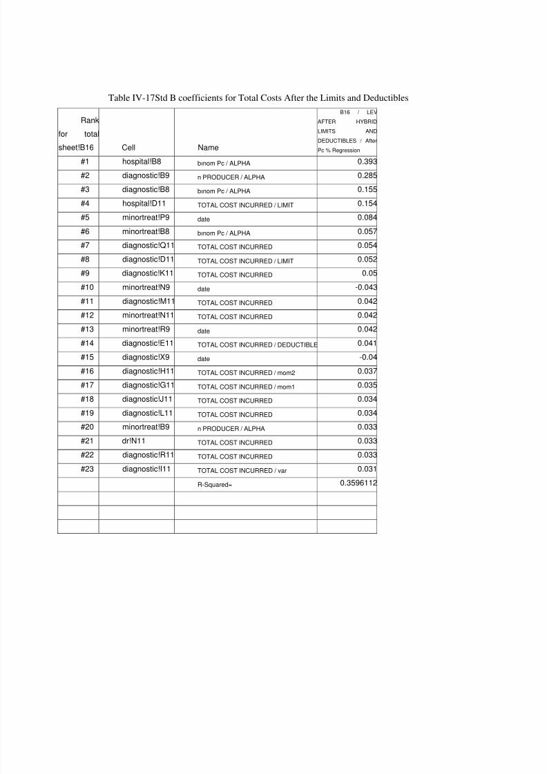
8/8/2019 Bulent Eris Model Development for Planning and Forecasting in Diagnostic and Treatment Systems 9022004
http://slidepdf.com/reader/full/bulent-eris-model-development-for-planning-and-forecasting-in-diagnostic-and 113/182
Table IV-17Std B coefficients for Total Costs After the Limits and Deductibles
Rank
for totalsheet!B16 Cell Name
B16 / LEVAFTER HYBRIDLIMITS ANDDEDUCTIBLES / AfterPc % Regression
#1 hospital!B8 bınom Pc / ALPHA 0.393#2 diagnostic!B9 n PRODUCER / ALPHA 0.285#3 diagnostic!B8 bınom Pc / ALPHA 0.155#4 hospital!D11 TOTAL COST INCURRED / LIMIT 0.154#5 minortreat!P9 date 0.084#6 minortreat!B8 bınom Pc / ALPHA 0.057#7 diagnostic!Q11 TOTAL COST INCURRED 0.054#8 diagnostic!D11 TOTAL COST INCURRED / LIMIT 0.052
#9 diagnostic!K11 TOTAL COST INCURRED 0.05#10 minortreat!N9 date -0.043#11 diagnostic!M11 TOTAL COST INCURRED 0.042#12 minortreat!N11 TOTAL COST INCURRED 0.042#13 minortreat!R9 date 0.042#14 diagnostic!E11 TOTAL COST INCURRED / DEDUCTIBLE 0.041#15 diagnostic!X9 date -0.04#16 diagnostic!H11 TOTAL COST INCURRED / mom2 0.037#17 diagnostic!G11 TOTAL COST INCURRED / mom1 0.035#18 diagnostic!J11 TOTAL COST INCURRED 0.034#19 diagnostic!L11 TOTAL COST INCURRED 0.034#20 minortreat!B9 n PRODUCER / ALPHA 0.033#21 dr!N11 TOTAL COST INCURRED 0.033#22 diagnostic!R11 TOTAL COST INCURRED 0.033#23 diagnostic!I11 TOTAL COST INCURRED / var 0.031 R-Squared= 0.3596112

8/8/2019 Bulent Eris Model Development for Planning and Forecasting in Diagnostic and Treatment Systems 9022004
http://slidepdf.com/reader/full/bulent-eris-model-development-for-planning-and-forecasting-in-diagnostic-and 114/182

8/8/2019 Bulent Eris Model Development for Planning and Forecasting in Diagnostic and Treatment Systems 9022004
http://slidepdf.com/reader/full/bulent-eris-model-development-for-planning-and-forecasting-in-diagnostic-and 115/182
Table V-1 Age an Gender characteristics of the Sample DataGENDER AGE Group 1 Group 2 Group 3
CHILD 0-4 0.09 0.10 0.13CHILD 5-9 0.04 0.05 0.09CHILD 10-14 0.03 0.03 0.04CHILD 15-19 0.01 0.01 0.01CHILD 20-24 0.01 0.01 0.01
0.00MALE 16-20 0.00 0.00 0.00MALE 21-25 0.06 0.05 0.02MALE 26-30 0.15 0.14 0.14MALE 31-35 0.08 0.09 0.14MALE 36-40 0.03 0.03 0.05
MALE 41-45 0.01 0.02 0.02MALE 46-50 0.01 0.01 0.01MALE 51-55 0.00 0.00 0.00MALE 56-60 0.00 0.00 0.00MALE 61-65 0.00 0.00 0.00MALE 66-70 0.00 0.00 0.00MALE 71-75 0.00 0.00 0.00
0.00FEMALE 16-20 0.00 0.00 0.00FEMALE 21-25 0.07 0.07 0.11
FEMALE 26-30 0.13 0.13 0.15FEMALE 31-35 0.08 0.08 0.09FEMALE 36-40 0.03 0.03 0.02FEMALE 41-45 0.01 0.01 0.00FEMALE 46-50 0.00 0.00 0.00FEMALE 51-55 0.00 0.00 0.00FEMALE 56-60 0.00 0.00 0.00FEMALE 61-65 0.00 0.00 0.00FEMALE 66-70 0.00 0.00 0.00FEMALE 71-75 0.00 0.00 0.00

8/8/2019 Bulent Eris Model Development for Planning and Forecasting in Diagnostic and Treatment Systems 9022004
http://slidepdf.com/reader/full/bulent-eris-model-development-for-planning-and-forecasting-in-diagnostic-and 116/182
V.1.1.2 Profile of Group 1
This group is formed of total members where the 0.58 of the total is employed by the
employer setting up the plan. There have been maximum 1607 members in the group andcosts are formed of records from 1999. This group is formed of white collar all over Turkey
who are on the mid and upper income class.
V.1.1.3 Profile of Group 2
This group is formed of total members where the 0.57 of the total is employed by the
employer setting up the plan. There have been maximum 1686 members in the group and
costs are formed of records from 2000. This group is formed of white collar all over Turkey
who are on the mid and upper income class.
V.1.1.4 Profile of Group 3
This group is formed of total members where the 0.36 of the total is employed by the
employer setting up the plan. There have been maximum 4143 members in the group and
costs are formed of records from 1999. this group is formed of white collar office
workers(from Istanbul) and sales representatives from allover Turkey, and in the second part
white collar and blue collar workers(from Anatolian non Ankara metropolitan)who are on themid and upper income class.
V.1.2 Scenarios
And scenario tested is provided as
Table V-2 Dr scenarios
DR LIMITS (all numbers in USD) SCNR1 SCNR2Number of Physician Visit Limit 4 10000Number of Physician Visit Deductible 0 0Per Physician Visit Limit 35 100Per Physician Visit Deductible 0 50

8/8/2019 Bulent Eris Model Development for Planning and Forecasting in Diagnostic and Treatment Systems 9022004
http://slidepdf.com/reader/full/bulent-eris-model-development-for-planning-and-forecasting-in-diagnostic-and 117/182
Table V-3 Prescription ScenariosPRES LIMITS SCNR1 SCNR2Number of Prescription Limit 4 10000Number of Physician Visit Deductible 0 0
Per Prescription Limit 35 100Per Prescription Deductible 0 50
Table V-4 Diagnostic Scenarios
DIAGNOSTIC LIMITS SCNR1 SCNR2Number of Diagnostic Proced. Limit 10000 10000Number of Diagnostic Proced. Deductible 0 0Annual Diagnostic Proced. Expense Total
Limit 150 2000
Annual Diagnostic Proced. Expense TotalDeductible 0 100
Table V-5 Minor Treatment Scenarios
MINORTREAT LIMITS SCNR1 SCNR2Number of Diagnostic Proced. Limit 10000 10000Number of Diagnostic Proced. Deductible 0 0Annual Diagnostic Proced. Expense Total Limit 500 2000Annual Diagnostic Proced. Expense Total Deductible 0 100
Table V-6 Hospital Scenarios
HOSPITAL LIMITS SCNR1 SCNR2Number of Hospitalization Limit 10000 10000Number of Hospitalization Deductible 0 0Annual Hospitalization Expense Total Limit 1500 30000Annual Hospitalization Expense Total
Deductible 0 1000

8/8/2019 Bulent Eris Model Development for Planning and Forecasting in Diagnostic and Treatment Systems 9022004
http://slidepdf.com/reader/full/bulent-eris-model-development-for-planning-and-forecasting-in-diagnostic-and 118/182
V.1.2.1 Output Analysis
V.1.2.1.1 Analysis on Benefit On Individual Total Cost
The analysis can only be done on individual basis (it is nearly impossible to find out 15-
20 years of a big group experience)
For the number of iterations 10,000 is chosen as it is above the number suggested by
@RISK. @RISK includes a convergence monitoring capability to help evaluate the stability
of the output distributions during a simulation. As more iterations are run, output distributions
become more "stable" as the statistics describing each distribution change less and less with
additional iterations. It is important to run enough iterations so that the statistics generated on
your outputs are reliable. However, there comes a point when the time spent for additionaliterations is essentially wasted because the statistics generated are not changing significantly.
Different random seed is used foe each simulation. Latin Hypercube is used for
sampling.

8/8/2019 Bulent Eris Model Development for Planning and Forecasting in Diagnostic and Treatment Systems 9022004
http://slidepdf.com/reader/full/bulent-eris-model-development-for-planning-and-forecasting-in-diagnostic-and 119/182

8/8/2019 Bulent Eris Model Development for Planning and Forecasting in Diagnostic and Treatment Systems 9022004
http://slidepdf.com/reader/full/bulent-eris-model-development-for-planning-and-forecasting-in-diagnostic-and 120/182

8/8/2019 Bulent Eris Model Development for Planning and Forecasting in Diagnostic and Treatment Systems 9022004
http://slidepdf.com/reader/full/bulent-eris-model-development-for-planning-and-forecasting-in-diagnostic-and 121/182
Mann-Whitney test
Table V-9 Mann-Whitney test for Gr1 Total CostsU 7,947,339U (expected value) 8,425,000U (variance) 16,279,997,479Z (observed value) -3.74Z (critical value) 3.89Two-tailed p-value 0Alpha 0.000
At the level of significance alpha=1.00E-04 the decision is to not reject the null
hypothesis of absence of difference between samples.
In other words, the difference between samples is not significant.
Table V-10 Kolmogorov-Smirnov test for Gr1 Total CostsD 0.213Two-tailed p-value < 0.0001Alpha 0.000
At the level of significance alpha=1.00E-04 the decision is to reject the null hypothesis
of absence of difference between samples.
In other words, the difference between samples is significant.
For the costs after all limits and deductibles for all benefits in scenarios below data is
gathered

8/8/2019 Bulent Eris Model Development for Planning and Forecasting in Diagnostic and Treatment Systems 9022004
http://slidepdf.com/reader/full/bulent-eris-model-development-for-planning-and-forecasting-in-diagnostic-and 122/182
Table V-11 Distribution of Group 1 After First Scenario
Sim real100 0.513 0.470
200 0.256 0.219
300 0.112 0.155400 0.056 0.081500 0.011 0.018600 0.010 0.011
700 0.005 0.005800 0.003 0.004900 0.004 0.004
1000 0.002 0.0021100 0.003 0.0011200 0.001 0.0011300 0.001 0.0021400 0.002 0.0031500 0.002 0.0021600 0.007 0.0041700 0.006 0.0021800 0.004 0.0081900 0.003 0.0062000 0.000 0.001
20000 0.000 0.001

8/8/2019 Bulent Eris Model Development for Planning and Forecasting in Diagnostic and Treatment Systems 9022004
http://slidepdf.com/reader/full/bulent-eris-model-development-for-planning-and-forecasting-in-diagnostic-and 123/182
Table V-12 Descriptive Stats of Group 1 After First Scenario
Real dataSimulation
data
Mean 187.89 167.15Standard Error 7.44 2.79Median 115.71 96.01Mode 0.00 0.00Standard Deviation 298.05 278.79Sample Variance 88,835.09 77,721.21Kurtosis 16.54 18.25Skewness 3.80 4.03Range 2,054.37 2,343.43Minimum 0.00 0.00Maximum 2,054.37 2,343.43Sum 301,937.72 1,671,533.99Count 1,607.00 10,000.00
0.000
0.100
0.200
0.300
0.400
0.500
0.600
1 0 0
3 0 0
5 0 0
7 0 0
9 0 0
1 1 0 0
1 3 0 0
1 5 0 0
1 7 0 0
1 9 0 0
2 0 0 0 0
Sim
real
Figure V.2 Graph of Group 1 After First Scenario
When we apply a chi-test
Ho: there are no significant differences between real & simulated freq.
H1: there are significant differences between real & simulated freq.
Statistical test: X2

8/8/2019 Bulent Eris Model Development for Planning and Forecasting in Diagnostic and Treatment Systems 9022004
http://slidepdf.com/reader/full/bulent-eris-model-development-for-planning-and-forecasting-in-diagnostic-and 124/182
Level of Significant : α=0.05
Rejection area which is the less than value of α =0.05
Ho: is rejected with 45.07 and critical value as 32.67
For other non parametric tests, we applied Mann-Whitney test / two-tailed test:
and the out put is
Table V-13 Mann-Whitney test for Gr. 1 Scen.1U 8,423,444U (expected value) 8,035,000
U (variance) 15,432,295,358Z (observed value) 3.13
Z (critical value) 3.89Two-tailed p-value 0Alpha 0.000
The Mann-Whitney's U is normalized and tested against the normal distribution
Decision:
At the level of significance alpha=1.00E-04 the decision is to not reject the null
hypothesis of absence of difference between samples.
In other words, the difference between samples is not significant.
Kolmogorov-Smirnov test / two-tailed test:
Table V-14 Kolmogorov-Smirnov test for Gr.1 and Scen. 1D 0.185Two-tailed p-value < 0.0001Alpha 0.000
Decision:
At the level of significance alpha=1.00E-04 the decision is to reject the null hypothesis
of absence of difference between samples.
In other words, the difference between samples is significant.

8/8/2019 Bulent Eris Model Development for Planning and Forecasting in Diagnostic and Treatment Systems 9022004
http://slidepdf.com/reader/full/bulent-eris-model-development-for-planning-and-forecasting-in-diagnostic-and 125/182
Table V-15 Descriptive Stats of Group 1 After Second Scenario
Real dataSimulation
data
Mean 93.82 102.18Standard Error 12.86 4.11Median 0.00 0.00Mode 0.00 0.00Standard Deviation 515.54 411.46Sample Variance 265,783.16 169,299.18Kurtosis 392.14 180.79Skewness 17.27 10.93Range 13,783.72 11,564.98Minimum 0.00 0.00Maximum 13,783.72 11,564.98Sum 150,769.37 1,021,842.60Count 1,607.00 10,000.00

8/8/2019 Bulent Eris Model Development for Planning and Forecasting in Diagnostic and Treatment Systems 9022004
http://slidepdf.com/reader/full/bulent-eris-model-development-for-planning-and-forecasting-in-diagnostic-and 126/182
Table V-16 Distribution of Group 1 After Second Scenario
Sim Real100 0.853 0.843
200 0.040 0.060
300 0.025 0.032400 0.017 0.017500 0.011 0.009600 0.010 0.009
700 0.008 0.004800 0.006 0.004900 0.005 0.002
1000 0.003 0.0011100 0.003 0.0021200 0.002 0.0021300 0.003 0.0011400 0.001 0.0011500 0.002 0.0011600 0.001 0.0011700 0.001 0.0011800 0.001 0.0021900 0.001 0.0012000 0.001 0.001
20000 0.007 0.007

8/8/2019 Bulent Eris Model Development for Planning and Forecasting in Diagnostic and Treatment Systems 9022004
http://slidepdf.com/reader/full/bulent-eris-model-development-for-planning-and-forecasting-in-diagnostic-and 127/182
0.000
0.1000.200
0.300
0.4000.500
0.600
0.7000.800
0.900
1 4 7 1 0
1 3
1 6
1 9
Sim
real
Figure V.3 Graph of Group 1 After Second Scenario
When we apply a chi-testHo: there are no significant differences between real & simulated freq.
H1: there are significant differences between real & simulated freq.
Statistical test: X2
Level of Significant : α=0.05
Rejection area which is the less than value of α =0.05
Ho: is rejected with 40.92 and critical value as 32.67
And for non parametrics
Table V-17 Mann-Whitney test for Gr. 1 Scen.2U 7,166,201.00U (expected value) 8,035,000.00U (variance) 13,187,253,313.25Z (observed value) -7.57Z (critical value) 3.89Two-tailed p-value < 0.0001Alpha 0.000
Decision: At the level of significance alpha=1.00E-04 the decision is to reject the nullhypothesis of absence of difference between samples.
In other words, the difference between samples is significant.

8/8/2019 Bulent Eris Model Development for Planning and Forecasting in Diagnostic and Treatment Systems 9022004
http://slidepdf.com/reader/full/bulent-eris-model-development-for-planning-and-forecasting-in-diagnostic-and 128/182
Table V-18 Kolmogorov-Smirnov test for Gr.3 and Scen. 2D 0.537Two-tailed p-value < 0.0001Alpha 0.000
At the level of significance alpha=1.00E-04 the decision is to reject the null hypothesis
of absence of difference between samples.
In other words, the difference between samples is significant.
V.1.2.1.1.2 Group 2
For the total costs incurred
Table V-19 Distribution of Group 2 Total Costs
Sim real100 0.441 0.510
200 0.180 0.162
300 0.109 0.089400 0.074 0.064500 0.046 0.038600 0.032 0.029
700 0.021 0.020800 0.017 0.016900 0.010 0.015
1000 0.009 0.0111100 0.008 0.0041200 0.007 0.0021300 0.004 0.0041400 0.006 0.0031500 0.004 0.0031600 0.003 0.0021700 0.003 0.0041800 0.003 0.0021900 0.002 0.0012000 0.003 0.003
20000 0.019 0.018

8/8/2019 Bulent Eris Model Development for Planning and Forecasting in Diagnostic and Treatment Systems 9022004
http://slidepdf.com/reader/full/bulent-eris-model-development-for-planning-and-forecasting-in-diagnostic-and 129/182
Table V-20 Descriptive Stats of Group 2 Total Costsreal sim
Mean 315.15 295.89Standard Error 45.69 5.88Median 95.08 126.37Mode 0.00 0.00Standard Deviation 1,875.42 588.07Sample Variance 3,517,206.60 345,822.03Kurtosis 1,261.22 74.78Skewness 33.55 6.67Range 71,833.54 12,523.14
Minimum 0.00 0.00Maximum 71,833.54 12,523.14Sum 531,026.66 2,958,873.56Count 1,685.00 10,000.00
0.000
0.100
0.200
0.3000.400
0.500
0.600
1 0 0
3 0 0
5 0 0
7 0 0
9 0 0
1 1 0 0
1 3 0 0
1 5 0 0
1 7 0 0
1 9 0 0
2 0 0 0 0
Sim
real
Figure V.4 Graph of Group 2 Total Costs
When we apply a chi-test
Ho: there are no significant differences between real & simulated freq.
H1: there are significant differences between real & simulated freq.
Statistical test: X2
Level of Significant : α=0.05

8/8/2019 Bulent Eris Model Development for Planning and Forecasting in Diagnostic and Treatment Systems 9022004
http://slidepdf.com/reader/full/bulent-eris-model-development-for-planning-and-forecasting-in-diagnostic-and 130/182
Rejection area which is the less than value of α =0.05
Ho: accepted with 27.33 and critical value as 32.67
Mann-Whitney test
Table V-21 Mann-Whitney test for Gr2 Total CostsU 7,947,465.00U (expected value) 8,425,000.00U (variance) 16,298,830,116.85Z (observed value) -3.74Z (critical value) 3.89Two-tailed p-value 0.00Alpha 0.000
At the level of significance alpha=1.00E-04 the decision is to not reject the null
hypothesis of absence of difference between samples.
In other words, the difference between samples is not significant.
Table V-22 Kolmogorov-Smirnov test for Gr2 Total CostsD 0.143
Two-tailed p-value < 0.0001Alpha 0.000
At the level of significance alpha=1.00E-04 the decision is to reject the null hypothesis
of absence of difference between samples.
In other words, the difference between samples is significant.
For the costs after all limits and deductibles for all benefits in scenarios below data is
gathered

8/8/2019 Bulent Eris Model Development for Planning and Forecasting in Diagnostic and Treatment Systems 9022004
http://slidepdf.com/reader/full/bulent-eris-model-development-for-planning-and-forecasting-in-diagnostic-and 131/182
Table V-23 Distribution of Group 2 After First Scenario
Sim real100 0.52 0.49
200 0.25 0.24
300 0.10 0.15400 0.06 0.05500 0.01 0.01600 0.01 0.00
700 0.01 0.01800 0.00 0.01900 0.00 0.00
1000 0.00 0.00
1100 0.00 0.001200 0.00 0.001300 0.00 0.001400 0.00 0.001500 0.00 0.001600 0.01 0.001700 0.01 0.001800 0.00 0.011900 0.00 0.002000 0.00 0.00
20000 0.00 0.00

8/8/2019 Bulent Eris Model Development for Planning and Forecasting in Diagnostic and Treatment Systems 9022004
http://slidepdf.com/reader/full/bulent-eris-model-development-for-planning-and-forecasting-in-diagnostic-and 132/182
Table V-24 Descriptive Stats of Group 2 After First Scenario
Real dataSimulation
data
Mean 179.98 166.02Standard Error 7.20 2.80Median 102.14 94.48Mode 0.00 0.00Standard Deviation 295.57 279.55Sample Variance 87,363.06 78,146.12Kurtosis 17.92 18.36Skewness 4.00 4.03Range 2,209.77 2,317.87Minimum 0.00 0.00Maximum 2,209.77 2,317.87Sum 303,268.07 1,660,178.96Count 1,685.00 10,000.00
0.00
0.10
0.200.30
0.40
0.50
0.60
1 0 0
3 0 0
5 0 0
7 0 0
9 0 0
1 1 0 0
1 3 0 0
1 5 0 0
1 7 0 0
1 9 0 0
2 0 0 0
0
Sim
real
Figure V.5 Graph of Group 2 After First Scenario
When we apply a chi-test
Ho: there are no significant differences between real & simulated freq.H1: there are significant differences between real & simulated freq.
Statistical test: X2
Level of Significant : α=0.05
Rejection area which is the less than value of α =0.05

8/8/2019 Bulent Eris Model Development for Planning and Forecasting in Diagnostic and Treatment Systems 9022004
http://slidepdf.com/reader/full/bulent-eris-model-development-for-planning-and-forecasting-in-diagnostic-and 133/182
Ho: is accepted with 28.07 and critical value as 32.67
For other non parametric tests, we applied Mann-Whitney test / two-tailed test:
and the out put is
Table V-25 Mann-Whitney test for Gr. 2 Scen.1U 8,877,201.00U (expected value) 8,425,000.00
U (variance) 16,307,707,507.21Z (observed value) 3.54Z (critical value) 3.89Two-tailed p-value 0.00Alpha 0.00
The Mann-Whitney's U is normalized and tested against the normal distribution
Decision:
At the level of significance alpha=1.00E-04 the decision is to not reject the null
hypothesis of absence of difference between samples.
In other words, the difference between samples is not significant.
Kolmogorov-Smirnov test / two-tailed test:
Table V-26 Kolmogorov-Smirnov test for Gr.2 and Scen. 1D 0.112Two-tailed p-value < 0.0001Alpha 0.000
Decision:
At the level of significance alpha=1.00E-04 the decision is to reject the null hypothesis
of absence of difference between samples.
In other words, the difference between samples is significant.

8/8/2019 Bulent Eris Model Development for Planning and Forecasting in Diagnostic and Treatment Systems 9022004
http://slidepdf.com/reader/full/bulent-eris-model-development-for-planning-and-forecasting-in-diagnostic-and 134/182
Table V-27 Descriptive Stats of Group 2 After Second Scenario
Real dataSimulation
data
Mean 84.83 100.12
Standard Error 21.34 4.06Median 0.00 0.00Mode 0.00 0.00Standard Deviation 876.11 405.93Sample Variance 767,561.70 164,780.07Kurtosis 832.91 189.21Skewness 26.73 10.99Range 29,764.68 11,440.17Minimum 0.00 0.00Maximum 29,764.68 11,440.17Sum 142,938.36 1,001,198.50Count 1,685.00 10,000.00

8/8/2019 Bulent Eris Model Development for Planning and Forecasting in Diagnostic and Treatment Systems 9022004
http://slidepdf.com/reader/full/bulent-eris-model-development-for-planning-and-forecasting-in-diagnostic-and 135/182

8/8/2019 Bulent Eris Model Development for Planning and Forecasting in Diagnostic and Treatment Systems 9022004
http://slidepdf.com/reader/full/bulent-eris-model-development-for-planning-and-forecasting-in-diagnostic-and 136/182
0.000
0.100
0.200
0.300
0.400
0.500
0.600
0.700
0.800
0.900
1.000
1 4 7 1 0
1 3
1 6
1 9
Sim
real
Figure V.6 Graph of Group 2 After Second Scenario
When we apply a chi-test
Ho: there are no significant differences between real & simulated freq.
H1: there are significant differences between real & simulated freq.
Statistical test: X2
Level of Significant : α=0.05
Rejection area which is the less than value of α =0.05
Ho: is accepted with 19.82 and critical value as 32.67
And for non parametrics
Table V-29 Mann-Whitney test for Gr. 1 Scen.2U 10,159,916.00U (expected value) 8,419,158.00U (variance) 13,727,428,725.43Z (observed value) 14.86Z (critical value) 3.89Two-tailed p-value < 0.0001Alpha 0.00
Decision: At the level of significance alpha=1.00E-04 the decision is to reject the null
hypothesis of absence of difference between samples.
In other words, the difference between samples is significant.
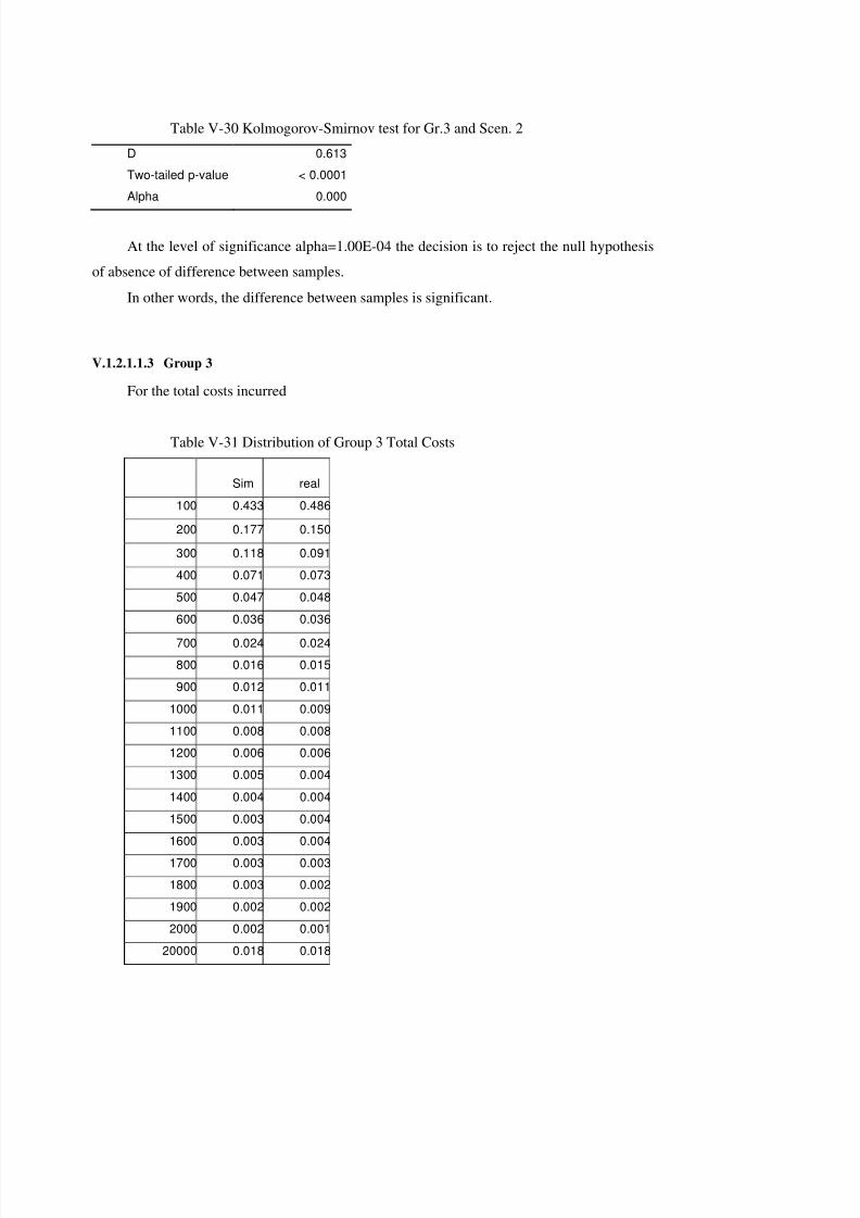
8/8/2019 Bulent Eris Model Development for Planning and Forecasting in Diagnostic and Treatment Systems 9022004
http://slidepdf.com/reader/full/bulent-eris-model-development-for-planning-and-forecasting-in-diagnostic-and 137/182
Table V-30 Kolmogorov-Smirnov test for Gr.3 and Scen. 2D 0.613Two-tailed p-value < 0.0001Alpha 0.000
At the level of significance alpha=1.00E-04 the decision is to reject the null hypothesis
of absence of difference between samples.
In other words, the difference between samples is significant.
V.1.2.1.1.3 Group 3
For the total costs incurred
Table V-31 Distribution of Group 3 Total Costs
Sim real100 0.433 0.486
200 0.177 0.150
300 0.118 0.091400 0.071 0.073500 0.047 0.048600 0.036 0.036
700 0.024 0.024800 0.016 0.015900 0.012 0.011
1000 0.011 0.0091100 0.008 0.0081200 0.006 0.0061300 0.005 0.0041400 0.004 0.0041500 0.003 0.0041600 0.003 0.0041700 0.003 0.0031800 0.003 0.0021900 0.002 0.0022000 0.002 0.001
20000 0.018 0.018
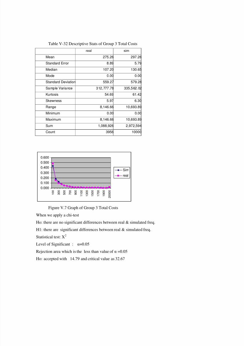
8/8/2019 Bulent Eris Model Development for Planning and Forecasting in Diagnostic and Treatment Systems 9022004
http://slidepdf.com/reader/full/bulent-eris-model-development-for-planning-and-forecasting-in-diagnostic-and 138/182
Table V-32 Descriptive Stats of Group 3 Total Costsreal sim
Mean 275.26 297.26Standard Error 8.89 5.79Median 107.20 130.65Mode 0.00 0.00Standard Deviation 559.27 579.28Sample Variance 312,777.78 335,562.02Kurtosis 54.69 61.42Skewness 5.97 6.30Range 8,146.66 10,693.89Minimum 0.00 0.00
Maximum 8,146.66 10,693.89Sum 1,088,926 2,972,594Count 3956 10000
0.0000.100
0.2000.3000.4000.5000.600
1 0 0
3 0 0
5 0 0
7 0 0
9 0 0
1 1 0 0
1 3 0 0
1 5 0 0
1 7 0 0
1 9 0 0
2 0 0 0 0
Sim
real
Figure V.7 Graph of Group 3 Total Costs
When we apply a chi-test
Ho: there are no significant differences between real & simulated freq.
H1: there are significant differences between real & simulated freq.
Statistical test: X2
Level of Significant : α=0.05Rejection area which is the less than value of α =0.05
Ho: accepted with 14.79 and critical value as 32.67

8/8/2019 Bulent Eris Model Development for Planning and Forecasting in Diagnostic and Treatment Systems 9022004
http://slidepdf.com/reader/full/bulent-eris-model-development-for-planning-and-forecasting-in-diagnostic-and 139/182
Mann-Whitney test
Table V-33 Mann-Whitney test for Gr3 Total CostsU 17,584,590U (expected value) 19,780,000U (variance) 45,381,441,883Z (observed value) -10.31Z (critical value) 3.89Two-tailed p-value < 0.0001Alpha 0.000
Decision: At the level of significance alpha=1.00E-04 the decision is to reject the null
hypothesis of absence of difference between samples.
In other words, the difference between samples is significant.
Table V-34 Kolmogorov-Smirnov test for Gr3 Total CostsD 0.231Two-tailed p-value < 0.0001Alpha 0.000
At the level of significance alpha=1.00E-04 the decision is to reject the null hypothesis
of absence of difference between samples.
In other words, the difference between samples is significant.
For the costs after all limits and deductibles for all benefits in scenarios below data is
gathered

8/8/2019 Bulent Eris Model Development for Planning and Forecasting in Diagnostic and Treatment Systems 9022004
http://slidepdf.com/reader/full/bulent-eris-model-development-for-planning-and-forecasting-in-diagnostic-and 140/182
Table V-35 Distribution of Group 3 After First Scenario
Sim real100 0.507 0.508
200 0.255 0.208
300 0.117 0.132400 0.058 0.068500 0.011 0.016600 0.009 0.009
700 0.005 0.007800 0.004 0.005900 0.002 0.006
1000 0.003 0.0041100 0.002 0.0041200 0.002 0.0041300 0.002 0.0021400 0.002 0.0031500 0.002 0.0021600 0.007 0.0041700 0.006 0.0051800 0.004 0.0051900 0.002 0.0042000 0.001 0.002
20000 0.001 0.003
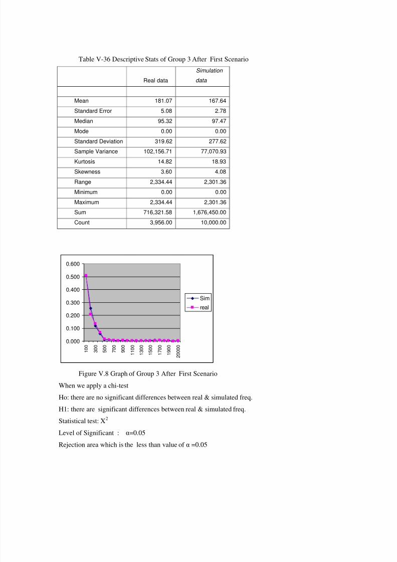
8/8/2019 Bulent Eris Model Development for Planning and Forecasting in Diagnostic and Treatment Systems 9022004
http://slidepdf.com/reader/full/bulent-eris-model-development-for-planning-and-forecasting-in-diagnostic-and 141/182
Table V-36 Descriptive Stats of Group 3 After First Scenario
Real dataSimulation
data
Mean 181.07 167.64Standard Error 5.08 2.78Median 95.32 97.47Mode 0.00 0.00Standard Deviation 319.62 277.62Sample Variance 102,156.71 77,070.93Kurtosis 14.82 18.93Skewness 3.60 4.08Range 2,334.44 2,301.36Minimum 0.00 0.00Maximum 2,334.44 2,301.36Sum 716,321.58 1,676,450.00Count 3,956.00 10,000.00
0.000
0.100
0.200
0.300
0.400
0.500
0.600
1 0 0
3 0 0
5 0 0
7 0 0
9 0 0
1 1 0 0
1 3 0 0
1 5 0 0
1 7 0 0
1 9 0 0
2 0 0 0 0
Sim
real
Figure V.8 Graph of Group 3 After First Scenario
When we apply a chi-test
Ho: there are no significant differences between real & simulated freq.H1: there are significant differences between real & simulated freq.
Statistical test: X2
Level of Significant : α=0.05
Rejection area which is the less than value of α =0.05

8/8/2019 Bulent Eris Model Development for Planning and Forecasting in Diagnostic and Treatment Systems 9022004
http://slidepdf.com/reader/full/bulent-eris-model-development-for-planning-and-forecasting-in-diagnostic-and 142/182
Ho: accepted with 28.73 and critical value as 32.67
For other non parametric tests, we applied Mann-Whitney test / two-tailed test:
and the out put is
Table V-37 Mann-Whitney test for Gr. 3 Scen.1U 18,496,837U (expected value) 19,780,000
U (variance) 45,381,209,438Z (observed value) -6.02Z (critical value) 3.89Two-tailed p-value < 0.0001Alpha 0.000
The Mann-Whitney's U is normalized and tested against the normal distribution
Decision:
At the level of significance alpha=1.00E-04 the decision is to reject the null hypothesis
of absence of difference between samples.
In other words, the difference between samples is significant.
Kolmogorov-Smirnov test / two-tailed test:
Table V-38 Kolmogorov-Smirnov test for Gr.3 and Scen. 1D 0.231Two-tailed p-value < 0.0001Alpha 0.000
At the level of significance alpha=1.00E-04 the decision is to reject the null hypothesis
of absence of difference between samples.
In other words, the difference between samples is significant.
Decision:

8/8/2019 Bulent Eris Model Development for Planning and Forecasting in Diagnostic and Treatment Systems 9022004
http://slidepdf.com/reader/full/bulent-eris-model-development-for-planning-and-forecasting-in-diagnostic-and 143/182
Table V-39 Descriptive Stats of Group 3 After Second ScenarioReal
dataSimulation
data
Mean 69 100Standard Error 5 4Median 0 0Mode 0 0Standard Deviation 322 401Sample Variance 103,957 160,845Kurtosis 156 135Skewness 11 10Range 6,670 9,484Minimum 0 0Maximum 6,670 9,484Sum 273,037 1,004,984Count 3,956 10,000

8/8/2019 Bulent Eris Model Development for Planning and Forecasting in Diagnostic and Treatment Systems 9022004
http://slidepdf.com/reader/full/bulent-eris-model-development-for-planning-and-forecasting-in-diagnostic-and 144/182
Table V-40 Distribution of Group 3 After Second Scenario
Sim Real
100 0.856 0.883200 0.043 0.039
300 0.024 0.023400 0.016 0.014500 0.011 0.008600 0.011 0.008
700 0.007 0.003800 0.004 0.004900 0.004 0.002
1000 0.003 0.0031100 0.003 0.0011200 0.002 0.0011300 0.001 0.0011400 0.002 0.0011500 0.001 0.0001600 0.001 0.0011700 0.002 0.0011800 0.001 0.0011900 0.001 0.001
2000 0.001 0.00120000 0.007 0.006

8/8/2019 Bulent Eris Model Development for Planning and Forecasting in Diagnostic and Treatment Systems 9022004
http://slidepdf.com/reader/full/bulent-eris-model-development-for-planning-and-forecasting-in-diagnostic-and 145/182
0.000
0.100
0.200
0.300
0.400
0.500
0.6000.700
0.800
0.900
1.000
1 4 7 1 0
1 3
1 6
1 9
Sim
real
Figure V.9 Graph of Group 3 After Second Scenario
When we apply a chi-test
Ho: there are no significant differences between real & simulated freq.
H1: there are significant differences between real & simulated freq.
Statistical test: X2
Level of Significant : α=0.05
Rejection area which is the less than value of α =0.05
Ho: accepted with 21.53 and critical value as 32.67
And for non parametrics
Table V-41 Mann-Whitney test for Gr. 3 Scen.2U 16,194,269.00U (expected value) 19,780,000.00U (variance) 37,703,780,245.16Z (observed value) -18.467Z (critical value) 3.891Two-tailed p-value < 0.0001
Alpha 0.000
Decision: At the level of significance alpha=1.00E-04 the decision is to reject the null
hypothesis of absence of difference between samples.
In other words, the difference between samples is significant.

8/8/2019 Bulent Eris Model Development for Planning and Forecasting in Diagnostic and Treatment Systems 9022004
http://slidepdf.com/reader/full/bulent-eris-model-development-for-planning-and-forecasting-in-diagnostic-and 146/182
Table V-42 Kolmogorov-Smirnov test for Gr.3 and Scen. 2D 0.427Two-tailed p-value < 0.0001Alpha 0.000
At the level of significance alpha=1.00E-04 the decision is to reject the null hypothesis
of absence of difference between samples.
In other words, the difference between samples is significant.
V.1.2.1.2 Analysis on Benefit Basis
In this part of the research we will look for an effect of scenerio2 to the mean claim size
per capita. To do this the first step to be taken is to construct a simulation data using the
restrictions determined for scenario2. Then the next step is to check whether the means of the
root populations of these samples are the same or not. Since we don’t know the population
variances we have to use T-test to check whether there exist a significant difference or not. At
this point there arises a problem: how can we estimate the variance of the differences of
sample means. There are two approaches to handle this problem. One is assuming the
population variances equal and using pooled variance as estimator of each population
variance and the other one is assuming population variances are not equal and use a weighted
variance as the variance of sample mean difference. To decide which approach to use we will
apply F test to sample variances. Let us now begin with the doctor expenses. First of all, we
begin with stating the null hypothesis H0: variances of two populations are equal and HA:
variances of two populations are not equal. The F test Output is given below.

8/8/2019 Bulent Eris Model Development for Planning and Forecasting in Diagnostic and Treatment Systems 9022004
http://slidepdf.com/reader/full/bulent-eris-model-development-for-planning-and-forecasting-in-diagnostic-and 147/182
Table V-43 F test for Physician Simulation and real data comparison
F-Test Two-Sample for
Variances
dr drsim
Mean 57.34699966 57.39982683Variance 7013.093549 5211.470245Observations 1989 7300df 1988 7299F 1.345703462P(F<=f) one-tail 6.98037E-18F Critical one-tail 1.060018295
Since the Calculated F value is greater than the tabulated one we reject the null
hypothesis, in other words we decide that there is a statistically significant difference between
two population variances. Now our next step is to apply T test with unequal variances
assumption. Here the sampling variation of the mean difference is the sum of variances each
divided by its sample size. The T test output is given below.

8/8/2019 Bulent Eris Model Development for Planning and Forecasting in Diagnostic and Treatment Systems 9022004
http://slidepdf.com/reader/full/bulent-eris-model-development-for-planning-and-forecasting-in-diagnostic-and 148/182
Table V-44 t test for Physician Simulation and real data comparison
t-Test: Two-Sample Assuming Unequal
Variances
dr drsim
Mean 57.34699966 57.39982683Variance 7013.093549 5211.470245Observations 1989 7300Hypothesized Mean Difference 0Df 2843t Stat -0.025655623P(T<=t) one-tail 0.48976691t Critical one-tail 1.645389602P(T<=t) two-tail 0.979533821t Critical two-tail 1.960797817
The absolute value of the calculated t value is less than the absolute value of the
tabulated one which means we don’t have any evidence to reject the null hypothesis claiming
the means are equal.
So we can say that at 95% level of confidence there is no evidence against our claim.
The scenario2 does not have an effect on doctor expenses. To visualize this more efficiently
we will now plot the real and simulated data on the same axis and compare them.

8/8/2019 Bulent Eris Model Development for Planning and Forecasting in Diagnostic and Treatment Systems 9022004
http://slidepdf.com/reader/full/bulent-eris-model-development-for-planning-and-forecasting-in-diagnostic-and 149/182
0
0.05
0.1
0.15
0.2
0.25
0.0001-20.0001
100.0001-120.0001
200.0001-220.0001
300.0001-320.0001
400.0001-420.0001
560.0001-580.0001
REAL DOCTORSIM DOCTOR
Figure V.10 Physician Visit Comparison
Graphical visualization is consistent with our findings. Two series differ from each
other in terms of dispersion but they seem to have similar means.
Now let us apply the same procedure to the prescription expenses. The F test output will
reveal if there exist any significant difference between variances of real and simulated
data.
Table V-45 F test for Prescribed Drugs Simulation and real data comparison
F-Test Two-Sample forVariances
pres pressim
Mean 36.24227677 36.543792Variance 4833.208537 2705.8660
27
Observations 1989 7300df 1988 7299F 1.786196541P(F<=f) one-tail 1.15318E-65F Critical one-tail 1.060018295

8/8/2019 Bulent Eris Model Development for Planning and Forecasting in Diagnostic and Treatment Systems 9022004
http://slidepdf.com/reader/full/bulent-eris-model-development-for-planning-and-forecasting-in-diagnostic-and 150/182
The result is similar to the one we did for doctor expenses. So we will use t test
assuming unequal. variances. The t test will look for any significant difference between
population means.
Table V-46 t test for Prescribed Drugs Simulation and real data comparison
t-Test: Two-Sample AssumingUnequal Variances
pres pressim
Mean 36.24227677 36.543792Variance 4833.208537 2705.866027Observations 1989 7300Hypothesized Mean Difference 0Df 2624t Stat -0.180169369P(T<=t) one-tail 0.428516759t Critical one-tail 1.645435077P(T<=t) two-tail 0.857033517t Critical two-tail 1.960870577
At 0,05 level of significance we cannot reject the equality of the means. So scenario2applied to prescription has no significant effect.
We will use a graphical visualization to check consistency of our results as we did for
doctor expenses

8/8/2019 Bulent Eris Model Development for Planning and Forecasting in Diagnostic and Treatment Systems 9022004
http://slidepdf.com/reader/full/bulent-eris-model-development-for-planning-and-forecasting-in-diagnostic-and 151/182
0
0.05
0.1
0.15
0.2
0.25
0 . 0 0
0 1 - 1 0
. 0 0 0 1
5 0 . 0 0
0 1 - 6 0
. 0 0 0 1
1 0 0 .
0 0 0 1
- 1 1 0 .
0 0 0 1
1 5 0 .
0 0 0 1
- 1 6 0 .
0 0 0 1
2 0 0 .
0 0 0 1
- 2 1 0
. 0 0 0 1
2 5 0 .
0 0 0 1
- 2 6 0
. 0 0 0 1
3 0 0 .
0 0 0 1
- 3 1 0 .
0 0 0 1
3 5 0 .
0 0 0 1
- 3 6 0 .
0 0 0 1
4 3 0 .
0 0 0 1
- 4 4 0
. 0 0 0 1
5 8 0 .
0 0 0 1
- 5 9 0 .
0 0 0 1
REAL PRESCRIBEDSIM PRESCRIBED
Figure V.11 Prescribed Drug Comparison
This graph again shows two populations differ only in terms of variability not in terms
of mean.
Now let us pass to application of the procedure to diagnostic expenses.
Starting with F test again we will decide whether to assume variances equal or not.
Table V-47 F test for Diagnostic Simulation and real data comparison
F-Test Two-Sample for
Variances
diag diagsim
Mean 35.82434506 40.65171246Variance 3232.504789 3866.209524Observations 1989 7300df 1988 7299F 1.196041
P(F<=f) one-tail 0.00000045F Critical one-tail 0.942297129
Te calculated F value is greater than the tabulated value so The conclusion is to reject
the equality of the variances.

8/8/2019 Bulent Eris Model Development for Planning and Forecasting in Diagnostic and Treatment Systems 9022004
http://slidepdf.com/reader/full/bulent-eris-model-development-for-planning-and-forecasting-in-diagnostic-and 152/182
Table V-48 t test for Diagnostic Simulation and real data comparison
t-Test: Two-Sample Assuming
Unequal Variances
diag diagsim
Mean 35.82434506 40.65171246Variance 3232.504789 3866.209524Observations 1989 7300Hypothesized Mean Difference 0df 3397t Stat -
3.288561699P(T<=t) one-tail 0.000508634t Critical one-tail 1.6453032P(T<=t) two-tail 0.001017267t Critical two-tail 1.960661393
The test come up with an unexpected result we rejected the null hypothesis stating the
equality of means so scenario2 applied to diagnostic expenses has a significant effect on the
mean claim size per capita.The graphical representation of this result is given below.

8/8/2019 Bulent Eris Model Development for Planning and Forecasting in Diagnostic and Treatment Systems 9022004
http://slidepdf.com/reader/full/bulent-eris-model-development-for-planning-and-forecasting-in-diagnostic-and 153/182
0
0.05
0.1
0.15
0.2
0.250.3
0.35
0.4
0.45
0 . 0 0
0 1 - 1 0
. 0 0 0 1
5 0 . 0 0
0 1 - 6 0
. 0 0 0 1
1 0 0 .
0 0 0 1
- 1 1 0 .
0 0 0 1
REAL DIAGNOSTICSIM DIAGNOSTIC
Figure V.12 Diagnostic procedure comparison
As it can be seen easily the two series do not resemble each other as we concluded in F
and t tests.
Now we will continue with minor treatment case. Again the first step is F test for
variances.
Table V-49 F test for Minor Treatment Simulation and real data comparison
F-Test Two-Sample forVariances
minor minorsim
Mean 12.15380529 10.06403624Variance 3370.709438 2992.406044Observations 1989 7300df 1988 7299
F 1.126421144P(F<=f) one-tail 0.000373858F Critical one-tail 1.060018295
As the calculated test statistic is greater than the tabulated one and since the F test is a
one tailed(right) test we conclude that the variances of two populations are different.

8/8/2019 Bulent Eris Model Development for Planning and Forecasting in Diagnostic and Treatment Systems 9022004
http://slidepdf.com/reader/full/bulent-eris-model-development-for-planning-and-forecasting-in-diagnostic-and 154/182

8/8/2019 Bulent Eris Model Development for Planning and Forecasting in Diagnostic and Treatment Systems 9022004
http://slidepdf.com/reader/full/bulent-eris-model-development-for-planning-and-forecasting-in-diagnostic-and 155/182
0
0.02
0.04
0.06
0.08
0.1
0.12
0.14
0.16
0.0001-10.0001
50.0001-60.0001
100.0001-110.0001
150.0001-160.0001
220.0001-230.0001
280.0001-290.0001
330.0001-340.0001
410.0001-420.0001
REAL MINORTREATSIM MINORTREAT
Figure V.13 Minor treatment comparison
A close look to the graph will reveal the same conclusion that we made for the tests.
Finally the last variable we will apply the same scenario is hospital expenses.
We again start with the F test.
Table V-51 F test for Hospital Simulation and real data comparison
F-Test Two-Sample forVariances
hosp hospsim
Mean 53.42372541 43.93490211Variance 75392.37087 54916.13154Observations 1989 7300df 1988 7299F 1.372863833P(F<=f) one-tail 3.56962E-20
F Critical one-tail 1.060018295
F test shows that the variances of two populations are different. So we will again use t
test for unequal variances.
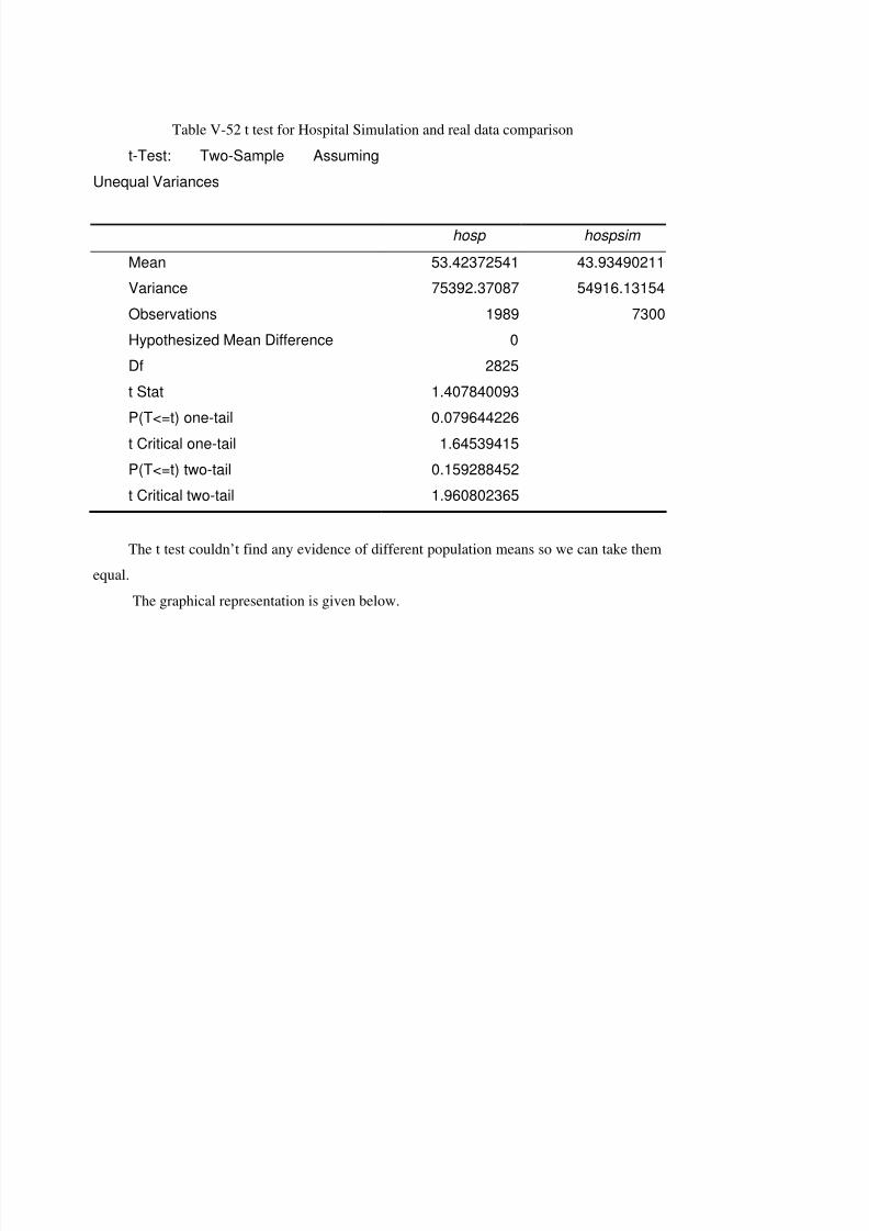
8/8/2019 Bulent Eris Model Development for Planning and Forecasting in Diagnostic and Treatment Systems 9022004
http://slidepdf.com/reader/full/bulent-eris-model-development-for-planning-and-forecasting-in-diagnostic-and 156/182
Table V-52 t test for Hospital Simulation and real data comparison
t-Test: Two-Sample AssumingUnequal Variances
hosp hospsim
Mean 53.42372541 43.93490211Variance 75392.37087 54916.13154Observations 1989 7300Hypothesized Mean Difference 0Df 2825t Stat 1.407840093P(T<=t) one-tail 0.079644226t Critical one-tail 1.64539415P(T<=t) two-tail 0.159288452t Critical two-tail 1.960802365
The t test couldn’t find any evidence of different population means so we can take them
equal.
The graphical representation is given below.

8/8/2019 Bulent Eris Model Development for Planning and Forecasting in Diagnostic and Treatment Systems 9022004
http://slidepdf.com/reader/full/bulent-eris-model-development-for-planning-and-forecasting-in-diagnostic-and 157/182
0 . 0 0
0 . 0 5
0 . 1 0
0 . 1 5
0 . 2 0
0 . 2 5
0 . 3 0
0 . 3 5
5 0 1
1 , 5 0 1
2 , 5 0 1
3 , 5 0 1
4 , 5 0 1
5 , 5 0 1
7 , 0 0 1
8 , 5 0 1
1 0 , 0 0
1
S im H o s p i ta lR e a l H o s p i ta l
Figure V.14 Hospital benefit comparisonIt is seen that the simulated series is less disperse than the original one and the mean is
more or less the same. Without applying tests we could have made the same conclusion.
To sum up at this section of the study we tried to show that there is no significant effect
of scenario2 to any of the expense variables mentioned above. Except for Diagnostic expenses
we accomplished our goal. The problem in the diagnostic expenses case may be the effect of
the experimented company. For the further stages of the study we will apply the same
procedure to the sampled 8 companies and that will be a more precise and can be generalized
to the whole companies insured.

8/8/2019 Bulent Eris Model Development for Planning and Forecasting in Diagnostic and Treatment Systems 9022004
http://slidepdf.com/reader/full/bulent-eris-model-development-for-planning-and-forecasting-in-diagnostic-and 158/182
PART.VI. CONCLUSION
This dissertation has showed that, as in every real life problem health care services are
formed of very complex structure and there are various approaches to model the problem.
We presented the first example of a simulation model to predict group health insurances
health care expenses in Turkey. Some approaches are outlined and some general actuarial
concepts are adopted to private health insurance including fast Fourier transformation,
moments approach.
As well as the published statistics, this study is based on the real data. Experience of
140,000 lives of 4 years has been used to describe the model with a large number of variables
so that reliable forecasts can be made. The module variables are set as; probability of claiming
(Pc), number of claims (n), claim size (X). For every utilization area (physician visits etc) and
for each variable(Pc, X and n), as every age/gender band has its own distribution, age band /
gender sub groups are created. Total number of distributions derived adds-up 435 and then,
moments of these distributions are provided in the thesis. While structuring the simulation
model, the interrelations between these variables are examined and Spearman correlation
matrix of the Pc and n variables are calculated and tested. Further to this characteristics of the
monthly and annual output distributions are analyzed.
The model is structured into three modules; Individual Expenses Module, Experience
and Credibility Module, Individual to Group Module

8/8/2019 Bulent Eris Model Development for Planning and Forecasting in Diagnostic and Treatment Systems 9022004
http://slidepdf.com/reader/full/bulent-eris-model-development-for-planning-and-forecasting-in-diagnostic-and 159/182
Individual Expenses Module outputs the distributional characteristics of one person
representing the overall group demographics after limits and deductibles applied using the
correlated input. In the Experience and Credibility Module, prior statistics of the model
variables of probability of claiming, number of claims and claim size for demographical
classes are used. Distributional characteristics of each benefit for each variable of the model
(Pc, n and X) are combined with the respective portfolio distribution characteristics. Structure
of full and partial credibility factor formula for each variable is also a new approach for this
area of health insurance.
Individual to Group Module is the part where the distribution output from the Individual
Expense Module is used and uncertainty due to statistical fluctuations, model and data
uncertainty is examined. It is nearly impossible to regenerate the results of one year with
identical conditions to see the overall risk spread in real life therefore this part of the model is
very useful to picture the stochastic nature of the aggregate costs.
In the Characteristics of the Model Output and Sensitivity section we examined the
characteristics that we cannot examine in real life, like effect of dependency, group size
(statistical fluctuation) and uncertainty due to factors mentioned in Individual to Group
Module. After examining these an overall sensitivity analysis is done to identify the most
critical inputs in the model with the limits and deductibles. The out come showed that the
limits and deductibles are decreasing the significance in the coefficients but do not change therank of significance among other variables. Further to this results show that Probability of
claiming (Pc) of hospitalization is the most critical value on the overall results.
The implementation of the model is illustrated on three sample groups with 7,436 lives
who had 59,080 health claims in total. For two different health insurance schemes (scenarios)
all the claims are filtered and compared with the simulation results with same demographic
out put limits and deductibles. Simulated results for total costs (from all areas of usage like
physician visits, hospital etc) and benefit-based costs are compared with actual costs of thesegroups. Although the output is made up of very complex combination of calculations, the
results are satisfactory.
As the model is structured on excel based simulation environment it is easy to
understand and to follow. Although non-technical people can use the model, great care should

8/8/2019 Bulent Eris Model Development for Planning and Forecasting in Diagnostic and Treatment Systems 9022004
http://slidepdf.com/reader/full/bulent-eris-model-development-for-planning-and-forecasting-in-diagnostic-and 160/182
be taken for keeping the model input data up to date. For example the unit costs should be
updated with current figures due to health inflation in USD. Also correcting the distribution
characteristics of the model variables or experience parameters great care should be taken for
the changes in the number of members of the exposed population. (If the number of members
of the exposed population changes in examined period, some elimination should be done for
the new comers.)
The model presented in this study is potentially a useful tool for helping a health
insurance company or private health fund to determine the risk characteristics that can be
faced while pricing and designing a health plan. By introducing the concept of credibility to
the distribution characteristics of the expenditure areas predictive accuracy of the model is
improved.
In addition to private health insurance, the issues that are explained in this study can be
used in areas stated below:
• Hospital groups will need advice on preferred provider arrangements. An
actuary with knowledge of health care demographics could forecast the demand
and likely case mix for a new hospital in a geographic region.
• Third party administrators for large group medical expenses plans and health aid
funds that are substitutive to social security will need advice for product design,
premium rating and reserving requirements. They also need advice on specificand aggregate stop loss insurance to limit their clients' exposure to catastrophic
(extremely big) claims.
• Large employers with insured medical expenses plans will need advice on
benefit plan design and the relative merits of competitive bids from a variety of
medical expenses insurers. The experience rating formulae used by different
insurers are not easily comparable; the lowest quoted premium may not result in
the lowest cost. An actuary can also advise on the likely effect of cost
containment measures designed to mitigate future increases in claim costs.
It will be interesting to see to which extent the private health insurance market in
Turkey will follow health insurance product developments in the U.S.A. These developments
might take the form of self funded medical trusts, ASO (Administrative Services Only)
contracts, HMOs (Health Maintenance Organizations) and PPOs (Preferred Provider

8/8/2019 Bulent Eris Model Development for Planning and Forecasting in Diagnostic and Treatment Systems 9022004
http://slidepdf.com/reader/full/bulent-eris-model-development-for-planning-and-forecasting-in-diagnostic-and 161/182
Organizations). Many of these developments might open up opportunities for modeling
involvement, particularly in the areas of risk management.
We believe that further studies are needed in this area. The model is built up for a
private health insurance population and that’s why congenital or chronic cases are less than a
public social insurance portfolio. The composition of such population should be examined
and credibility module should be used if only short-term data is available for these sources
before adopting the model to social security applications.

8/8/2019 Bulent Eris Model Development for Planning and Forecasting in Diagnostic and Treatment Systems 9022004
http://slidepdf.com/reader/full/bulent-eris-model-development-for-planning-and-forecasting-in-diagnostic-and 162/182
REFERENCES
[1]. Actuarial Standards Board Measuring Retiree Group Benefit Obligations USA(2001)13-27
[2]. Agency for Health Care Policy and Research Center for Cost and FinancingStudies “Medical Expenditure Panel Survey Household Component: Public Use File”Rockville, MD, USA (1997)
[3]. American Academy of Actuaries “Recommendations for Actuarial Advice GivenWith Respect to Self-Insured Employee Benefit Plans”, Washinton DC, USA,(1985)
[4]. Alexander, D.; Hilary N.; Shah S.:” Private Medical Insurance” Institute of Actuaries, London, UK,(2001)
[5]. Ash, A. S. ;Byrne-Logan, S.:“How well do models work? Predicting health carecosts” , in Proceedings of the Section on Statistics in Epidemiology, AmericanStatistical Association,.(1998)42-49
[6]. Barney, H. L.; Doran, P.; Rosenblatt, A.; Yamanoto, D.: “A Review of PremiumEstimates in the Health Security Act” American Academy of Actuaries, WashintonDC, USA (1994)
[7]. Bluhm, W.; Perkins, P.; Carstens, J.; Knapp, A.: “Actuarial Solvency Issues of Health Plans in the United States”(1994) [8]. Bluhm, W.: ”The Small Group Pricing Simulator
“http://www.milliman.com/minneapolis/tools/small_group_pricing_simulator.aspMilliman-USA Minnesota, USA
[9]. Board of Directors of the CAS: ‘Statement of Principles Regarding Property andCasualty Insurance Ratemaking’,(1988)
[10]. Daykin, C. D.; Pentikainen, T.; Pesonen., M.:“Practical Risk Theory for Actuaries” . Chapman and Hall, Washinton DC, USA,(1996)61
[11]. Dederichs, W.: “Claims Reserves in Health Assurances” Paper Presented to theSociety of Actuaries (of Turkey) II International Seminar on Health Insurance,Istanbul, Turkey,(1992)
[12]. Dullaway, D.: “Experience Rating of Medical Expense Insurance” The ActuaryLondon UK(1992)
[13]. Fleischacker, P.; Discenza, J.; Huey, M.; “Actuarial Issues Related to PrizingHealth plans Under Health Care Reform” American Academy of Actuaries,Washinton DC, USA,(1994)
[14]. Glas, J.: “Application of Deductibles and their effects” Paper Presented to theSociety of Actuaries (of Turkey) II International Seminar on Health Insurance,Istanbul, Turkey,(1992)
Comment [B4]:
Edwin C. Hustead, PeterHendee, Roland E. KingE.Litow, Gerald R. SheaL. Sutton Jr.,George. WaJr ‘Medical Savings AccCost Implications and DeIssues’ ,American AcadeActuaries ,1995(V1SLTSMedical Savings A c c oCost implications and DeIssues.pdf)
Board of Directors of the ‘Statement of Principles RProperty and Casualty InsRatemaking’, 1988(sppcrateStatement of PrinRegarding Property and CInsurance Ratemaking.pdf
Paul R. Fleischacker, JudiDiscenza, Martin S. Huey‘Actuarial Issues Related Prizing Health plans Unde
Care Reform’ American Aof Actuaries,1994(PRICINHEALTH PLANS.pdf veyPRICING HEALTH PLARISK2.pdf)(daha cok grup buyuklugdegil ama grup icindeki ygruplarının oranındanbahsediyor ama yararlı oozellikle Appendix kısmHarold L Barney, Phyllis Alice F Rosenblatt, Dale HYamanoto, A Review of PEstimates in the Health SeAct, 1994(PREMIUMESTIMATES.pdf)(Features that affect Primve Methodology kısmı g‘MEPS HC-003:1996 Pan
Population CharacteristicsUtilization Data’ , 1996(PPopulation CharacteristicsUtilization Data for 1996XXXXX.pdf)
‘Medical Expenditure PanSurvey Household CompoPublic Use File 1’, 1997(mexpenditure population chXXXXX.pdf)
‘Recommendations for AAdvice Given With RespeSelf-Insured Employee BePlans’, 1985(recomandatiactuarial adice given with to self insured employee bplans.pdf)
William F Bluhm, Peter PJanet M Carstens, Alan DActuarial Solvency IssuesHealth Plans in the United1994 (HEALTH PLANSOLVENCY.pdf)(Who takes the Risk veManaging the Risk bolumgenel bilgi verilen bir bokullanılabilir)Julia T Philips, Janet M C

8/8/2019 Bulent Eris Model Development for Planning and Forecasting in Diagnostic and Treatment Systems 9022004
http://slidepdf.com/reader/full/bulent-eris-model-development-for-planning-and-forecasting-in-diagnostic-and 163/182
[15]. Grazier, K.L., G’Sell Associates,“Group Medical Insurance Large Claims Database Collection and Analysis” American Academy of Actuaries, Washinton DC,USA, (1997)
[16]. Hauboldt, R.H.: “Cost Implications of Human Organ and Tissue Transplantations,an update: 1999”, Milliman & Robertson, Inc. Seattle, USA,(1999)
[17]. Hogg, R.; Klugman S.:“Loss Distributions” , John Wiley &Sons, New York,USA,(1984) [18]. Hossack, I. B.“Introductory Statistics with Applications in General Insurance”
Cambridge University Press, London, UK,(1983) [19]. Hustead, E.; Hendee, P.; King, R.; Litow, M., Shea, G.; Sutton, H.; Wagoner, G.;
“Medical Savings Accounts Cost Implications and Design Issues” , AmericanAcademy of Actuaries, Washinton DC, USA,(1995)
[20]. Klugman, S.; Panjer,H., Willmot, G.: ”Loss Models” John Wiley and Sons NewYork, USA,(1998) 605
[21]. Ministry of Health”Health Service Utilization Survey in Turkey”, Ankara, urkey, (1995).
[22]. MEPS HC-003:1996 Panel Population Characteristics and Utilization Data , 1996[23]. Mosslakos, E.; Thompson, S.: “Voluntary Health Insurance in the European Union
“Copenhagen, Denmark(2002) [24]. Newhouse, J.P.; Manning, W.G.; Keeler, E.B.; Sloss, E.M.:“Adjusting capitation
rates using objective health measurers and prior utilization” , Health Care FinancingReview, 10(3):(1989)41-54.
[25]. Orros, G.; Webber, J.: “Medical Expense Insurance- An Actuarial Review”Presented to the Institute of Actuaries, London, UK,(1987)
[26]. Orros, G. : “Group Medical Expenses in the United Kingdom” Benefits &Compensation International May(1985)
[27]. Palsbo, S.:”Risk Assessment and Risk Adjustment: A Field Guide for People with Disabilities” The National Institute of Disability and Rehabilitation Research(NIDRR) December, (2001)
[28]. Philips, J. P.; Carstens, J. P.; Lewis, L.; Swanson, S.; Zwitter, N.: “StandardBenefits in Health Care Reform-The Impact and Cost” American Academy of Actuaries, Washinton DC, USA,(1993)
[29]. Savas,B.Serdar et al.In Thomson,S.and Mossialos, E., eds.”Health care systems intransition: Turkey. Copenhagen, Copenhagen, Denmark(2002)
[30]. Seminar description “Modernizing Our Ancient Pricing Methods” 2003 S. MSnow & Associates, Inc.http://www.smsnow.com/Sem_AncientPricing/APmain.htm#detailed Berlin, MAUSA (2003)
[31]. Van de Ven; W.P.M.M., Ellis, R.P.:”Risk adjustment in competitive health planmarkets” . Handbook of Health Economics. A.J. Culyer and J.P. Newhouse, ElsevierScience B.V. 1A:(2000)755 – 845
[32]. Van de Ven, W.P.M.M.; van Vliet, R.C.J.A.:“How can we prevent cream
skimming in a competitive health insurance market? The great challenge for the‘90’s” , in P. Zweifel and H.E. French, eds., Health Economics World-wide KluwerAcademic Publishers, the Netherlands,(1992)23-46.
[33]. Walling, R.; “Managed Care: A Brief Look at the Past” Paper Presented to theCasualty Actuarial Society Ratemaking Seminar Nashville, USA,(1999)
[34]. Wang, S.: “Aggregation of Correlated Risk Portfolios: Models & Algorithms”.Proceedings of the Casualty Actuarial Society,(1999)28

8/8/2019 Bulent Eris Model Development for Planning and Forecasting in Diagnostic and Treatment Systems 9022004
http://slidepdf.com/reader/full/bulent-eris-model-development-for-planning-and-forecasting-in-diagnostic-and 164/182
[35]. Zhao, Y., Ellis, R.P., Ash, A.S., Calabrese, D., Ayanian, J.A., Slaughter, J.P.,Weyuker, L., Bowen, B., “Measuring Population Health Risks Using Inpatient
Diagnoses and Outpatient Pharmacy Data” HSR: Health Services Research, Part II,(2001)

8/8/2019 Bulent Eris Model Development for Planning and Forecasting in Diagnostic and Treatment Systems 9022004
http://slidepdf.com/reader/full/bulent-eris-model-development-for-planning-and-forecasting-in-diagnostic-and 165/182
APPENDIX 1
Definiton of the Actuary
An actuary is a professional businessperson skilled in the application of mathematics to
financial problems.
An actuary applies specialized knowledge of the mathematics of finance, statistics and
risk theory to problems faced by:
• Insurance companies
• Pension plans
• Government regulators
• Social programs
• Individuals
Traditionally, actuaries have specialized in:
• Life insurance
• Annuities
• Property and casualty insurance
• Pension plans
• Other employee benefit plans
• Evidence in the courts about loss of future earnings
An actuary has a practical business sense, the creativity to apply training and experience
to new problems and provide innovative solutions, and the communication skills required to

8/8/2019 Bulent Eris Model Development for Planning and Forecasting in Diagnostic and Treatment Systems 9022004
http://slidepdf.com/reader/full/bulent-eris-model-development-for-planning-and-forecasting-in-diagnostic-and 166/182
convince both colleagues and clients. Actuaries help people plan better for the future by
controlling or reducing financial risks associated with:
• Sickness• Disability
• Dying too soon
• Living too long
• Unemployment
• Property loss and damage
• Investment policy
Some actuaries spend part of their time ensuring that companies and pension plans
comply with the consumer protection and tax legislation, which govern their operations. In
legislation, an actuary is defined as a member of an institute, as a profession, have rules of
professional conduct and standards of practice.
The actuarial profession has played a significant role in the process of health insurance
and it is hoped that the role will strengthen over time. The primary areas of responsibility of
an actuary with a carrier organization would be, among others:
Pricing of contribution
Determination of reserves
Determination of reinsurance arrangement
Advice on benefit design
Determination of capital requirements
Pricing and advise on provider remuneration arrangements
Analysis of claims data
In order for the actuary to perform these tasks professionally and efficiently an
understanding of the dynamics within the health care environment is required.
Members of Actuarial Profession have become the highest income class mathematicians
who are employed in various sectors of finance as well as insurance and risk management.
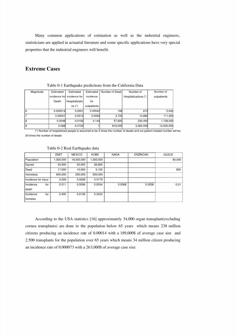
8/8/2019 Bulent Eris Model Development for Planning and Forecasting in Diagnostic and Treatment Systems 9022004
http://slidepdf.com/reader/full/bulent-eris-model-development-for-planning-and-forecasting-in-diagnostic-and 167/182
Many common applications of estimation as well as the industrial engineers,
statisticians are applied in actuarial literature and some specific applications have very special
properties that the industrial engineers will benefit.
Extreme Cases
Table 0-1 Earthquake predictions from the California DataMagnitude Estimated
incidence forDeath
Estimatedincidence forHospitalizatio
ns (*)
Estimatedincidence
foroutpatients
Number of Dead Number ofHospitalizations (*)
Number ofoutpatients
6 0.000014 0.0001 0.00042 168 672 5,0407 0.00031 0.0012 0.0093 3,720 14,880 111,6008 0.0048 0.0192 0.144 57,600 230,400 1,728,0009 0.068 0.2720 1 816,000 3,264,000 12,000,000
(*) Number of hospitalized people is assumed to be 4 times the number of deads and out patient treated number will be30 times the number of deads
Table 0-2 Real Earthquake dataIZMIT MEXCO KOBE NADA ERZNCAN DÜZCE
Population 1,500,000 18,000,000 1,500,000 80,000njured 43,000 50,000 26,800Dead 17,000 10,000 5,100 800Homeless 600,000 250,000 500,000Incidence for injury 0.029 0.0028 0.0179Incidence fordeath
0.011 0.0006 0.0034 0.0068 0.0058 0,01
Incidence forhomelss
0.400 0.0139 0.3333
According to the USA statistics [16] approximately 34,000 organ transplant(excluding
cornea transplants) are done to the population below 65 years which means 238 million
citizens producing an incidence rate of 0.00014 with a 189,000$ of average case size and
2,500 transplants for the population over 65 years which means 34 million citizen producing
an incidence rate of 0.000073 with a 263,000$ of average case size.

8/8/2019 Bulent Eris Model Development for Planning and Forecasting in Diagnostic and Treatment Systems 9022004
http://slidepdf.com/reader/full/bulent-eris-model-development-for-planning-and-forecasting-in-diagnostic-and 168/182
In Grazier K.L[15], depending on Group Private Insurance data USA, for all the large
medical expenditure cases below data is produced
Table 0-3 High costs incidence rates
AGE EXPOSEDNUMBER
AVERAGECOST
POSSIBILITYOF EXCEEDING25.000$
AVERAGECOST
POSSIBILITYOF EXCEEDING250.000$
0 20 317,319 46,246 0.004264 167,163 0.00016421 30 237,034 38,213 0.002536 145,546 0.00007231 40 362,143 39,294 0.003361 136,827 0.00007741 50 303,184 36,217 0.005700 132,088 0.00010251 60 169,052 31,556 0.014138 116,429 0.00018361 64 52,064 29,776 0.025680 98,078 0.00019265 69 32,655 25,195 0.016628 164,821 0.000092
70 120 44,774 25,628 0.010430 21,888 0.000067

8/8/2019 Bulent Eris Model Development for Planning and Forecasting in Diagnostic and Treatment Systems 9022004
http://slidepdf.com/reader/full/bulent-eris-model-development-for-planning-and-forecasting-in-diagnostic-and 169/182
APPENDIX 2
In the model there are 8 major sheets. The major sheets where all the iterations are done
are ‘dr’, ‘pres’,’ diagnostic’, ‘minortreat’, ’ hospital’ SHEETS
The formulas are
FORMULAS FROM RANGE B4:E7
B4. =+G4/C4
C4. =+I4/G4
B5. =+G5/C5
C5. =+I5/G5
B7. =+'YAŞ C NS YET'!T1
FORMULAS FROM RANGE G4:I5G4. =+'YAŞ C NS YET'!V1
H4. =+'YAŞ C NS YET'!W1
I4. =+H4-G4^2
G5. =+'YAŞ C NS YET'!X1
H5. =+'YAŞ C NS YET'!Y1
I5. =+H5-G5^2
FORMULAS FROM RANGE B8:B9
B8. =RiskBinomial(1, B7, RiskCorrmat(NewMatrixPc,1))
B9. =RiskOutput() + ROUND(RiskGamma(B4, C4,
RiskCorrmat(NewMatrixadet,1)),0)
FORMULAS FROM RANGE D9:AB9

8/8/2019 Bulent Eris Model Development for Planning and Forecasting in Diagnostic and Treatment Systems 9022004
http://slidepdf.com/reader/full/bulent-eris-model-development-for-planning-and-forecasting-in-diagnostic-and 170/182
D9. =+ IF(D11=0,0,RiskDiscrete($AD$2:$AD$13,$AE$2:$AE$13))
AB9. =+ IF(AB11=0,0,RiskDiscrete($AD$2:$AD$13,$AE$2:$AE$13))
FORMULAS FROM RANGE B12:C14
B12. =RiskOutput() + IF(B8=1,C12,0)
C12. =RiskOutput() + SUM(D12:AB12)
B14. =RiskOutput() + IF(B8=1,C14,0)
C14. =RiskOutput() + MAX(D14:AB14)
FORMULAS FROM RANGE B16:B21
B16. =RiskOutput() + RiskGamma($B$5,$C$5)
B17. =RiskOutput() +IF(B16>$D$5,$D$5-$E$5,IF(B16>$E$5,B16-$E$5,0))
B20. =RiskOutput() + IF(E11>$D$5,$D$5-$E$5,IF(E11>$E$5,E11-$E$5,0))
B21. =RiskOutput() + COUNTIF(D12:AB12,">0")
FORMULAS FROM RANGE D11:AB19
From D column to AB column below formulas are coppied
D11. =IF(D10>$B$9,0,RiskGamma($B$5,$C$5))
D12. =IF(D10>$D$4,0,IF(D10<=$E$4,0,IF(D11>$D$5,$D$5-
$E$5,IF(D11>$E$5,D11-$E$5,0))))
D13. =SUM($D$11:D11)
D14. =+IF(ISERROR(D15),0,D15)
D15. =+IF(D13<$E$6,0,IF(D13<$D$6,D13,$D$6)-$E$6)
D16. =+D11*(1-(MAX(D11-$D$5,0)/D11))-($E$5/D11)
D17. =+(D13-$E$6)*(1-(MAX(D11-$D$5,0)/D11))-($E$5/D11)
D18. =+($D$6-C13)*(1-(MAX(D11-$D$5,0)/D11))-($E$5/D11)
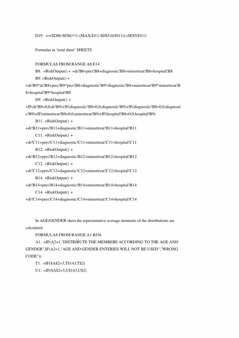
8/8/2019 Bulent Eris Model Development for Planning and Forecasting in Diagnostic and Treatment Systems 9022004
http://slidepdf.com/reader/full/bulent-eris-model-development-for-planning-and-forecasting-in-diagnostic-and 171/182
D19. =+($D$6-$E$6)*(1-(MAX(D11-$D$5,0)/D11))-($E$5/D11)
Formulas in ‘total sheet’ SHEETS
FORMULAS FROM RANGE A8:E14
B8. =RiskOutput() + +dr!B8+pres!B8+diagnostic!B8+minortreat!B8+hospital!B8
B9. =RiskOutput() +
+dr!B9*dr!B8+pres!B9*pres!B8+diagnostic!B9*diagnostic!B8+minortreat!B9*minortreat!B
8+hospital!B9*hospital!B8
D9. =RiskOutput() +
+IF(dr!B8=0,0,dr!B9)+IF(diagnostic!B8=0,0,diagnostic!B9)+IF(diagnostic!B8=0,0,diagnosti
c!B9)+IF(minortreat!B8=0,0,minortreat!B9)+IF(hospital!B8=0,0,hospital!B9)
B11. =RiskOutput() +
+dr!B11+pres!B11+diagnostic!B11+minortreat!B11+hospital!B11
C11. =RiskOutput() +
+dr!C11+pres!C11+diagnostic!C11+minortreat!C11+hospital!C11
B12. =RiskOutput() +
+dr!B12+pres!B12+diagnostic!B12+minortreat!B12+hospital!B12
C12. =RiskOutput() +
+dr!C12+pres!C12+diagnostic!C12+minortreat!C12+hospital!C12
B14. =RiskOutput() ++dr!B14+pres!B14+diagnostic!B14+minortreat!B14+hospital!B14
C14. =RiskOutput() +
+dr!C14+pres!C14+diagnostic!C14+minortreat!C14+hospital!C14
In AGE/GENDER sheet the representative average moments of the distributions are
calculated.
FORMULAS FROM RANGE A1:BJ36A1. =IF(A2=1,"DISTRIBUTE THE MEMBERS ACCORDING TO THE AGE AND
GENDER",IF(A2=1,"AGE AND GENDER ENTERIES WILL NOT BE USED","WRONG
CODE"))
T1. =IF($A$2=3,T$143,T$2)
U1. =IF($A$2=3,U$143,U$2)

8/8/2019 Bulent Eris Model Development for Planning and Forecasting in Diagnostic and Treatment Systems 9022004
http://slidepdf.com/reader/full/bulent-eris-model-development-for-planning-and-forecasting-in-diagnostic-and 172/182
V1. =IF($A$2=3,V$143,V$2)
W1. =IF($A$2=3,W$143,W$2)
X1. =IF($A$2=3,X$143,X$2)
Y1. =IF($A$2=3,Y$143,Y$2)
AC1. =IF($A$2=3,AC$143,AC$2)
AD1. =IF($A$2=3,AD$143,AD$2)
AE1. =IF($A$2=3,AE$143,AE$2)
AF1. =IF($A$2=3,AF$143,AF$2)
AG1. =IF($A$2=3,AG$143,AG$2)
AH1. =IF($A$2=3,AH$143,AH$2)
AL1. =IF($A$2=3,AL$143,AL$2)
AM1. =IF($A$2=3,AM$143,AM$2)
AN1. =IF($A$2=3,AN$143,AN$2)
AO1. =IF($A$2=3,AO$143,AO$2)
AP1. =IF($A$2=3,AP$143,AP$2)
AQ1. =IF($A$2=3,AQ$143,AQ$2)
AU1. =IF($A$2=3,AU$143,AU$2)
AV1. =IF($A$2=3,AV$143,AV$2)
AW1. =IF($A$2=3,AW$143,AW$2)
AX1. =IF($A$2=3,AX$143,AX$2)
AY1. =IF($A$2=3,AY$143,AY$2)AZ1. =IF($A$2=3,AZ$143,AZ$2)
BD1. =IF($A$2=3,BD$143,BD$2)
BE1. =IF($A$2=3,BE$143,BE$2)
BF1. =IF($A$2=3,BF$143,BF$2)
BG1. =IF($A$2=3,BG$143,BG$2)
BH1. =IF($A$2=3,BH$143,BH$2)
BI1. =IF($A$2=3,BI$143,BI$2)
T2. =SUMPRODUCT($E$6:$E$142,T6:T142)U2. =SUMPRODUCT($E$6:$E$142,U6:U142)
V2.
=SUMPRODUCT($E$6:$E$36,T6:T36,V6:V36)/SUMPRODUCT($E$6:$E$36,T6:T36)
W2.
=SUMPRODUCT($E$6:$E$36,T6:T36,W6:W36)/SUMPRODUCT($E$6:$E$36,T6:T36)

8/8/2019 Bulent Eris Model Development for Planning and Forecasting in Diagnostic and Treatment Systems 9022004
http://slidepdf.com/reader/full/bulent-eris-model-development-for-planning-and-forecasting-in-diagnostic-and 173/182
X2.
=SUMPRODUCT($E$6:$E$36,T6:T36,V6:V36,X6:X36)/SUMPRODUCT($E$6:$E$36,V6:
V36,T6:T36)
Y2.
=SUMPRODUCT($E$6:$E$36,T6:T36,V6:V36,Y6:Y36)/SUMPRODUCT($E$6:$E$36,V6:
V36,T6:T36)
AC2. =SUMPRODUCT($E$6:$E$142,AC6:AC142)
AD2. =SUMPRODUCT($E$6:$E$142,AD6:AD142)
AE2.
=SUMPRODUCT($E$6:$E$36,AC6:AC36,AE6:AE36)/SUMPRODUCT($E$6:$E$36,AC6:
AC36)
AF2.
=SUMPRODUCT($E$6:$E$36,AC6:AC36,AF6:AF36)/SUMPRODUCT($E$6:$E$36,AC6:
AC36)
AG2.
=SUMPRODUCT($E$6:$E$36,AC6:AC36,AE6:AE36,AG6:AG36)/SUMPRODUCT($E$6:
$E$36,AE6:AE36,AC6:AC36)
AH2.
=SUMPRODUCT($E$6:$E$36,AC6:AC36,AE6:AE36,AH6:AH36)/SUMPRODUCT($E$6:
$E$36,AE6:AE36,AC6:AC36)
AL2. =SUMPRODUCT($E$6:$E$142,AL6:AL142)AM2. =SUMPRODUCT($E$6:$E$142,AM6:AM142)
AN2.
=SUMPRODUCT($E$6:$E$36,AL6:AL36,AN6:AN36)/SUMPRODUCT($E$6:$E$36,AL6:
AL36)
AO2.
=SUMPRODUCT($E$6:$E$36,AL6:AL36,AO6:AO36)/SUMPRODUCT($E$6:$E$36,AL6:
AL36)
AP2.=SUMPRODUCT($E$6:$E$36,AL6:AL36,AN6:AN36,AP6:AP36)/SUMPRODUCT($E$6:$
E$36,AN6:AN36,AL6:AL36)
AQ2.
=SUMPRODUCT($E$6:$E$36,AL6:AL36,AN6:AN36,AQ6:AQ36)/SUMPRODUCT($E$6:
$E$36,AN6:AN36,AL6:AL36)

8/8/2019 Bulent Eris Model Development for Planning and Forecasting in Diagnostic and Treatment Systems 9022004
http://slidepdf.com/reader/full/bulent-eris-model-development-for-planning-and-forecasting-in-diagnostic-and 174/182
AU2. =SUMPRODUCT($E$6:$E$142,AU6:AU142)
AV2. =SUMPRODUCT($E$6:$E$142,AV6:AV142)
AW2.
=SUMPRODUCT($E$6:$E$36,AU6:AU36,AW6:AW36)/SUMPRODUCT($E$6:$E$36,AU
6:AU36)
AX2.
=SUMPRODUCT($E$6:$E$36,AU6:AU36,AX6:AX36)/SUMPRODUCT($E$6:$E$36,AU6
:AU36)
AY2.
=SUMPRODUCT($E$6:$E$36,AU6:AU36,AW6:AW36,AY6:AY36)/SUMPRODUCT($E$
6:$E$36,AW6:AW36,AU6:AU36)
AZ2.
=SUMPRODUCT($E$6:$E$36,AU6:AU36,AW6:AW36,AZ6:AZ36)/SUMPRODUCT($E$6
:$E$36,AW6:AW36,AU6:AU36)
BD2. =SUMPRODUCT($E$6:$E$142,BD6:BD142)
BE2. =SUMPRODUCT($E$6:$E$142,BE6:BE142)
BF2.
=SUMPRODUCT($E$6:$E$36,BD6:BD36,BF6:BF36)/SUMPRODUCT($E$6:$E$36,BD6:
BD36)
BG2.
=SUMPRODUCT($E$6:$E$36,BD6:BD36,BG6:BG36)/SUMPRODUCT($E$6:$E$36,BD6:BD36)
BH2.
=SUMPRODUCT($E$6:$E$36,BD6:BD36,BF6:BF36,BH6:BH36)/SUMPRODUCT($E$6:$
E$36,BF6:BF36,BD6:BD36)
BI2.
=SUMPRODUCT($E$6:$E$36,BD6:BD36,BF6:BF36,BI6:BI36)/SUMPRODUCT($E$6:$E
$36,BF6:BF36,BD6:BD36)
AE3.=SUMPRODUCT($E$6:$E$36,AC6:AC36,AE6:AE36)/SUMPRODUCT($E$6:$E$36,AC6:
AC36)
AF3.
=SUMPRODUCT($E$6:$E$36,AC6:AC36,AF6:AF36)/SUMPRODUCT($E$6:$E$36,AC6:
AC36)

8/8/2019 Bulent Eris Model Development for Planning and Forecasting in Diagnostic and Treatment Systems 9022004
http://slidepdf.com/reader/full/bulent-eris-model-development-for-planning-and-forecasting-in-diagnostic-and 175/182

8/8/2019 Bulent Eris Model Development for Planning and Forecasting in Diagnostic and Treatment Systems 9022004
http://slidepdf.com/reader/full/bulent-eris-model-development-for-planning-and-forecasting-in-diagnostic-and 176/182
APPENDIX 3
Fourier Algorithm
Sub Macro1()
'
' Macro1 Macro' Macro recorded 11.06.2000
'
Application.Run "ATPVBAEN.XLA!Fourier", ActiveSheet.Range("$B$2:$B$33"),
_
ActiveSheet.Range("$N$2:$N$33"), False, False
End Sub
Sub fftsht()Dim found As Integer, row As Integer
Dim s As String, power As Integer
found = False
row = 5
Workbooks.Open FileName:="C:\Fourier\inputfile.xls"
While Not found
row = row + 1
s = "I" & Trim$(Str$(row))
If Workbooks("inputfile.xls").Worksheets("tablolar").Range(s) = "Grand Total"
Then found = True
Wend
power = Int(Log(row - 6) / Log(2)) + 1
For i = 1 To 2 ^ power
8/8/2019 Bulent Eris Model Development for Planning and Forecasting in Diagnostic and Treatment Systems 9022004
http://slidepdf.com/reader/full/bulent-eris-model-development-for-planning-and-forecasting-in-diagnostic-and 177/182

8/8/2019 Bulent Eris Model Development for Planning and Forecasting in Diagnostic and Treatment Systems 9022004
http://slidepdf.com/reader/full/bulent-eris-model-development-for-planning-and-forecasting-in-diagnostic-and 178/182
Workbooks("fftsht.xls").Worksheets("n-fold").Range(Chr$(65 + row) & "2:" & Chr$(65 +
row) & Trim$(Str$(2 ^ power + 1))).Value
Workbooks("fftsht.xls").Worksheets("n-fold").Range(Chr$(67 + row) & "2:" &
Chr$(67 + row) & Trim(Str$(2 ^ power + 1))).Formula = "=IMPRODUCT(" & Chr$(65 +
row) & "2," & Chr$(66 + row) & "2)"
For i = 2 To row - 2
Application.Run "ATPVBAEN.XLA!Fourier",
Workbooks("fftsht.xls").Worksheets("n-fold").Range("$" & Chr$(67 + row) & "$2:$" &
Chr$(67 + row) & "$" & Trim(Str$(2 ^ power + 1))), _
Workbooks("fftsht.xls").Worksheets("n-fold").Range("$" & Chr$(68 + row) &
"$2:$" & Chr$(68 + row) & "$" & Trim(Str$(2 ^ power + 1))), True, False
Workbooks("fftsht.xls").Worksheets("n-fold").Range(Chr$(65 + i) & "2:" &
Chr$(65 + i) & Trim$(Str$(2 ^ power + 1))).Value = Workbooks("fftsht.xls").Worksheets("n-
fold").Range(Chr$(68 + row) & "2:" & Chr$(68 + row) & Trim$(Str$(2 ^ power + 1))).Value
Workbooks("fftsht.xls").Worksheets("n-fold").Range("$" & Chr$(68 + row) &
"$2:$" & Chr$(68 + row) & "$" & Trim(Str$(2 ^ power + 1))).ClearContentsWorkbooks("fftsht.xls").Worksheets("n-fold").Range("$" & Chr$(65 + row) &
"$2:$" & Chr$(65 + row) & "$" & Trim(Str$(2 ^ power + 1))).ClearContents
Application.Run "ATPVBAEN.XLA!Fourier",
Workbooks("fftsht.xls").Worksheets("n-fold").Range("$" & Chr$(65 + i) & "$2:$" &
Chr$(65 + i) & "$" & Trim(Str$(2 ^ power + 1))), _
Workbooks("fftsht.xls").Worksheets("n-fold").Range("$" & Chr$(65 + row) &
"$2:$" & Chr$(65 + row) & "$" & Trim(Str$(2 ^ power + 1))), False, FalseNext i
Workbooks("fftsht.xls").Worksheets("n-fold").Range("B" & Trim$(Str$(2 ^ power +
4))).Formula = "=B" & "$" & Trim$(Str$(2 ^ power + 3)) & "*B2"
Workbooks("fftsht.xls").Worksheets("n-fold").Range("B" & Trim$(Str$(2 ^ power +
4))).Copy

8/8/2019 Bulent Eris Model Development for Planning and Forecasting in Diagnostic and Treatment Systems 9022004
http://slidepdf.com/reader/full/bulent-eris-model-development-for-planning-and-forecasting-in-diagnostic-and 179/182
Workbooks("fftsht.xls").Worksheets("n-fold").Range("B" & Trim$(Str$(2 ^ power +
4)) & ":" & Chr$(63 + row) & Trim$(Str$((2 ^ power) * 2 + 4))).Select
ActiveSheet.Paste
Workbooks("fftsht.xls").Worksheets("n-fold").Range(Chr$(63 + row + 1) &
Trim$(Str$((2 ^ power) + 4)) & ":" & Chr$(63 + row + 1) & Trim$(Str$((2 ^ power) * 2 +
4))).Formula = "=SUM(B" & Trim$(Str$((2 ^ power) + 4)) & ":" & Chr$(63 + row) &
Trim$(Str$((2 ^ power) + 4)) & ")"
End Sub
Sub Macro2()
'
' Macro2 Macro
' Macro recorded 11.06.2000
'
'
Application.Run "ATPVBAEN.XLA!Fourier", ActiveSheet.Range("$T$2:$T$33"),
_
ActiveSheet.Range("$U$2:$U$33"), True, False
End Sub

8/8/2019 Bulent Eris Model Development for Planning and Forecasting in Diagnostic and Treatment Systems 9022004
http://slidepdf.com/reader/full/bulent-eris-model-development-for-planning-and-forecasting-in-diagnostic-and 180/182
CURRICULUM VITAE
Name: SALIH BULENT ERISHOME TEL:+90 216 3 40 37 35MOBILE TEL:+90 532 794 22 74E MAIL: [email protected]: BEYAZ KARANFIL SOKAK 19/8 ACIBADEM 81010ISTANBUL/TURKEYGENDER: MALEBIRTH DATE : DECEMBER,3RD 1967
EDUCATION1979-1985 KADIKÖY ANADOLU LISESI/ KADIKÖY ANADOLU SECONDARY-HIGHSCHOOL1985-1989 BS. IN MANAGEMENT ENGINEERING TECHNICAL UNIVERSITY,ISTANBUL (GRADUATION PROJECT: “CASH FLOW MANAGEMENT ANALYSIS”)1989-1992 MS. IN MARM. UNIV. BANKING AND INSURANCE FACULTY ININSURANCE (GRADUATION PROJECT: “MAJOR MEDICAL EXPENSE ANDUNLIMITED HEALTH INSURANCE BENEFITS”)EXPERIENCE1990-1996 Worked as specialist in System Research and Development department in chargeof actuarial subjects on life and health product development, system analysis1996-1999 MANAGER IN “TECHNICAL AND R&D” DEPARTMENT. ABOVESUBJECTS PLUS THE RE-INSURANCE AND POOLING WORK.1999- SENIOR MANAGERATTENDED SEMINARS ON VARIOUS SUBJECTS SUCH ASMARCH 1992 LIFE INSURANCE UNDERWRITING SEMINAR (FROM MUNICH RE)1994 AND 1995 2 MAIN COURSES FOR ISO 9001SEPTEMBER 1995 EDUCATION OF THE EDUCATORS (FROM ROTACONSULTANCY INC.)JUNE 1995 REACHING THE STARS (FROM TIME MANAGEMENT INTERNATIONALINC.)JUNE 1997 ACTUARIAL COURSE FOR ONE WEEK IN COLOGNEOCTOBER 2000 MAY 2001 MANAGEMENT TRAINING. (BY INTERCON)MARITAL STATUS
MARRIED SINCE 1991 AND HAS SON BORN JULY, 3RD 1995.

8/8/2019 Bulent Eris Model Development for Planning and Forecasting in Diagnostic and Treatment Systems 9022004
http://slidepdf.com/reader/full/bulent-eris-model-development-for-planning-and-forecasting-in-diagnostic-and 181/182
Page 143: [1] Comment [B4] BERIS
Edwin C. Hustead, Peter G. Hendee, Roland E. King, Mark E.Litow,Gerald R. Shea, Harry L. Sutton Jr.,George. Wagoner Jr ‘Medical SavingsAccounts Cost Implications and Design Issues’ ,American Academy of Actuaries ,1995 (V1SLTSL1 Medical Savings A c c o u n t s Costimplications and Design Issues.pdf)
Board of Directors of the CAS ‘Statement of Principles Regarding Property and CasualtyInsurance Ratemaking’, 1988(sppcrateStatement of Principles Regarding Property andCasualty Insurance Ratemaking.pdf)
Paul R. Fleischacker, Judith A. Discenza, Martin S. Huey, ‘Actuarial Issues Related to PrizingHealth plans Under Health Care Reform’ American Academy of Actuaries,1994(PRICINGHEALTH PLANS.pdf veya PRICING HEALTH PLAN RISK2.pdf)(daha cok grup buyuklugunden degil ama grup icindeki yas gruplarının oranındanbahsediyor ama yararlı olabilir ozellikle Appendix kısmı)Harold L Barney, Phyllis A Doran, Alice F Rosenblatt, Dale H Yamanoto, A Review of Premium Estimates in the Health Security Act, 1994(PREMIUM ESTIMATES.pdf)(Features that affect Primiums ve Methodology kısmı guzel)‘MEPS HC-003:1996 Panel Population Characteristics and Utilization Data’ , 1996(PanelPopulation Characteristics and Utilization Data for 1996 XXXXX.pdf)
‘Medical Expenditure Panel Survey Household Component: Public Use File 1’, 1997(medical expenditure population charac XXXXX.pdf)
‘Recommendations for Actuarial Advice Given With Respect to Self-Insured EmployeeBenefit Plans’, 1985(recomandations for actuarial adice given with respect to self insuredemployee benefit plans.pdf)
William F Bluhm, Peter Perkins, Janet M Carstens, Alan D Knapp, ‘ Actuarial SolvencyIssues of Health Plans in the United States’ 1994(HEALTH PLAN SOLVENCY.pdf)(Who takes the Risk ve Managing the Risk bolumleri genel bilgi verilen bir bolumdekullanılabilir)Julia T Philips, Janet M Carstens, Lucinda Lewis, Sheree Swanson, Norman Zwitter, ‘Standard Benefits in Health Care Reform-The Impact and Cost’ 1993(EFFEC OF standarthealth benefis IN USA.pdf)(Sizin calısmanıza benzer bir calısma bu calısmada 4 ayrı model simule edilmis ve buplanlar costları ile kıyaslanmıs)
Bunların dısında hcir.pdf de bulunan Health Care Index Report u , factse 50facts of health.pdf
dosyasında bulunan 50 Facts of Health yazısı ve monthly HMO premiums for singl e
premium.pdf de bulunan prim örnekleri konu anlatımı sırasında kullanılabilir gibi duruyor.

8/8/2019 Bulent Eris Model Development for Planning and Forecasting in Diagnostic and Treatment Systems 9022004
http://slidepdf.com/reader/full/bulent-eris-model-development-for-planning-and-forecasting-in-diagnostic-and 182/182