bulk temperature measurement in thermally striped pipe flows

NUREG/GR-0015

Bulk Temperature Measurement in Thermally Striped Pipe Flows

RECEIVED A06 0 5 figs OSTi

Prepared by N. Lemure, J. R. Olvera, A. E. Ruggles

College of Engineering The University of Tennessee

Prepared for U.S. Nuclear Regulatory Commission

MAST! DISTRIBUTION OF THIS DOCUMENT IS UNLIMITED

w

AVAILABILITY NOTICE

Availability of Reference Materials Cited in NRC Publications

Most documents cited in NRC publications will be available from one of the following sources:

1. The NRC Public Document Room, 2120 L Street, NW., Lower Level, Washington, DC 20555-0001

2. The Superintendent of Documents, U.S. Government Printing Office, P. O. Box 37082, Washington, DC 20402-9328

3. The National Technical Information Service, Springfield, VA 22161-0002

Although the listing that follows represents the majority of documents cited in NRC publications, it is not intended to be exhaustive.

Referenced documents available for inspection and copying for a fee from the NRC Public Document Room include NRC correspondence and Internal NRC memoranda; NRC bulletins, circulars, information notices, inspection and investigation notices; licensee event reports; vendor reports and correspondence; Commission papers; and applicant and licensee documents and correspondence.

The following documents in the NUREG series are available for purchase from the Government Printing Office: formal NRC staff and contractor reports, NRC-sponsored conference proceedings, international agreement reports, grantee reports, and NRC booklets and brochures. Also available are regulatory guides, NRC regulations in the Code of Federal Regulations, and Nuclear Regulatory Commission Issuances.

Documents available from the National Technical Information Service include NUREG-series reports and technical reports prepared by other Federal agencies and reports prepared by the Atomic Energy Commission, forerunner agency to the Nuclear Regulatory Commission.

Documents available from public and special technical libraries include all open literature items, such as books, journal articles, and transactions. Federal Register notices, Federal and State legislation, and congressional reports can usually be obtained from these libraries.

Documents such as theses, dissertations, foreign reports and translations, and non-NRC conference proceedings are available for purchase from the organization sponsoring the publication cited.

Single copies of NRC draft reports are available free, to the extent of supply, upon written request to the Office of Administration, Distribution and Mail Services Section, U.S. Nuclear Regulatory Commission, Washington, DC 20555-0001.

Copies of industry codes and standards used in a substantive manner in the NRC regulatory process are maintained at the NRC Library, Two White Flint North, 11545 Rockville Pike, Rockville, MD 20852-2738, for use by the public. Codes and standards are usually copyrighted and may be purchased from the originating organization or, if they are American National Standards, from the American National Standards Institute, 1430 Broadway, New York, NY 10018-3308.

DISCLAIMER NOTICE

This document was prepared with the support of the U.S. Nuclear Regulatory Commission (NRC) Grant Program. The purpose of the NRC Grant Program is to support basic, advanced, and developmental scientific research for a public purpose in areas relating to nuclear safety. The nature of NRC's Grant Program is such that the grantee bears prime responsibility for the conduct of the research and exercises judgement and original thought toward attaining the scientific goals. The opinions, findings, conclusions, and recommendations expressed herein are therefore those of the authors and do not necessarily reflect the views of the NRC.

NUREG/GR-0015

Bulk Temperature Measurement in Thermally Striped Pipe Flows

Manuscript Completed: November 1995 Date Published: December 1995

Prepared by N. Lemure, J. R. Olvera, A. E. Ruggles

College of Engineering The University of Tennessee Knoxville, TN 37996-2300

F. Eltawila, NRC Project Manager

Prepared for Division of Systems Technology Office of Nuclear Regulatory Research U.S. Nuclear Regulatory Commission Washington, DC 20555-0001 NRC Job Code G2530

For sale by the U.S. Government Printing Office Superintendent of Documents, Mail Stop: SSOP, Washington, DC 20402-9328

ISBN 0-16-048546-0

DISCLAIMER

Portions of this document may be illegible in electronic image products. Images are produced from the best available original document.

DISCLAIMER

This report was prepared as an account of work sponsored by an agency of the United States Government. Neither the United States Government nor any agency thereof, nor any of their employees, makes any warranty, express or implied, or assumes any legal liability or responsibility for the accuracy, completeness, or usefulness of any information, apparatus, product, or process disclosed, or represents that its use would not infringe privately owned rights. Reference herein to any specific commercial product, process, or service by trade name, trademark, manufacturer, or otherwise does not necessarily constitute or imply its endorsement, recommendation, or favoring by the United States Government or any agency thereof. The views and opinions of authors expressed herein do not necessarily state or reflect those of the United States Government or any agency thereof.

ABSTRACT

The bulk temperature measurement of pipe flows with thermal striping is explored. An experiment is conducted to examine the feasibility of using temperature measurements on the external surface of the pipe to estimate the bulk temperature of the flow. Simple mixing models are used to characterize the development of the temperature profile in the flow. Simple averaging techniques and Backward Propagating Neural Net are used to predict bulk temperature from the external temperature measurements. Accurate bulk temperatures can be predicted. However, some temperature distributions in the flow effectively mask the bulk temperature from the wall and cause significant error in the bulk temperature predicted using this technique.

iii

TABLE OF CONTENTS

Section

ABSTRACT

LIST OF TABLES

LIST OF FIGURES

Page

ill

Vll

Vlll

XI EXECUTIVE SUMMARY

1. INTRODUCTION 1.1 History of Thermal Striping in PWR Hot Legs 2 1.2 Determination of Bulk Temperature in PWR Hot Legs 4

2. EXPERIMENT OBJECTIVES AND DESIGN 2.1 Experiment Objectives 8 2.2 Description of the Thermal Stratification Test

Facility (TSTF) 9 2.3 System Operat .on 20

3. EXPERIMENT RESULTS AND OBSERVATIONS 3.1 Description of the TSTF Test Program 22 3.2 Characteristic TSTF Process Conditions 22 3.3 Description of the Experimental Results 2 5

3.3.1 Inlet Geometry I - Semi-Circular Inlet 26 3.3.2 Inlet Geometry II - Concentric Inlet 34 3.3.3 Inlet Geometry III - Off-Center Inlet 39

ANALYTICAL APPROACH TO BULK TEMPERATURE ESTIMATION OF THERMALLY STRIPED FLOWS 4.1 Principle Influences on External Temperature Distribution

4.2 Internal Temperature Distributions 4.2.1 Temperature Distribution for the Concentric

Inlet Condition

4.2.2 Temperature Distribution for the Semi-Circular Inlet Condition

4.2.3 Effective Thermal Diffusivity due to Turbulence

4.3 Heat Transfer Through the Pipe Wall

4.4 External Temperature Distributions

47 50

50

53 58 59 61

EMPIRICAL METHODS FOR PREDICTING BULK TEMPERATURE 5.1 Introduction 5.2 Statistical Method 5.3 Artificial Neural Networks

64 65 72

CONCLUSIONS 75

APPENDICES

Appendix A Appendix B Appendix C Appendix D Appendix E Appendix F

Duke Power Meeting Attendees Sensor Calibration Sample of Raw Data Post-Processing Background on Turbulence and Mixing Theory Background on Artificial Neural Networks Pipe Wall Thermal Transient

vi

LIST OF TABLES

Table Description Page

2-1 Thermocouple Positions 18 2-2 Extension Spool Pieces 20 3-1 Thermal Stratification Test Matrix 23 3-2 Supply Leg Flow Rate Ratios 24 5-1 External Thermocouple Groups 65 5-2 Desired vs. Predicted Bulk Temperature from Neural

Network Model 74

VII

LIST OF FIGURES

Figure Description Page

2-1 Thermal Stratification Test Facility 10 2-2 Inlet Condition Geometries Used in the TSTF 12 2-3 Inlet Mixing Piece I 13 2-4 Inlet Mixing Piece II 13 2-5 Test Spool Piece Installed in the TSTF 16 2-6 Thermocouple Harness 19 2-7 Thermocouple Probe 19 3-1 Internal Temperatures for Semi-Circular Inlet, HC Stations 27 3-2 External Temperatures for Semi-Circular Inlet, HC Stations 27 3-3 Internal Standard Deviations, Semi-Circular Inlet,

HC Stations 29 3-4 External Standard Deviations, Semi-Circular Inlet,

HC Stations 29 3-5 Internal Temperatures for Semi-Circular Inlet, CH Stations 31 3-6 External Temperatures for Semi-Circular Inlet, CH Stations 31 3-7 Internal Standard Deviations, Semi-Circular Inlet,

CH Stations 33 3-8 External Standard Deviations, Semi-Circular Inlet,

CH Stations 33 3-9 Internal Temperatures for Concentric Inlet, HC Stations 35 3-10 External Temperatures for Concentric Inlet, HC Stations 35 3-11 Internal Standard Deviations, Concentric Inlet, HC Stations 37 3-12 External Standard Deviations, Concentric Inlet, HC Stations 37 3-13 Internal Temperatures for Concentric Inlet, CH Stations 38 3-14 External Temperatures for Concentric Inlet, CH Stations 38 3-15 Internal Standard Deviations, Concentric Inlet, CH Stations 40 3-16 External Standard Deviations, Concentric Inlet, CH Stations 40 3-17 Internal Temperatures for Off-Center Inlet, Selected

HC Stations 42 3-18 External Temperatures for Off-Center Inlet, Selected

HC Stations 42 viii

LIST OF FIGURES (cont'd)

Figure Description Page

3-19 Internal Standard Deviations, Off-Center Inlet, Selected HC Stations 43

3-20 External Standard Deviations, Off-Center Inlet, Selected HC Stations 43

3-21 Internal Temperature Distributions at 5 m/s and 8 m/s, Station CHI 45

3-22 External Temperature Distributions at 5 m/s and 8 m/s, Station CHI 45

3-23 Internal Temperature Distributions at 5 m/s and 8 m/s, Station CH6 46

3-24 External Temperature Distributions at 5 m/s and 8 m/s, Station CH6 46

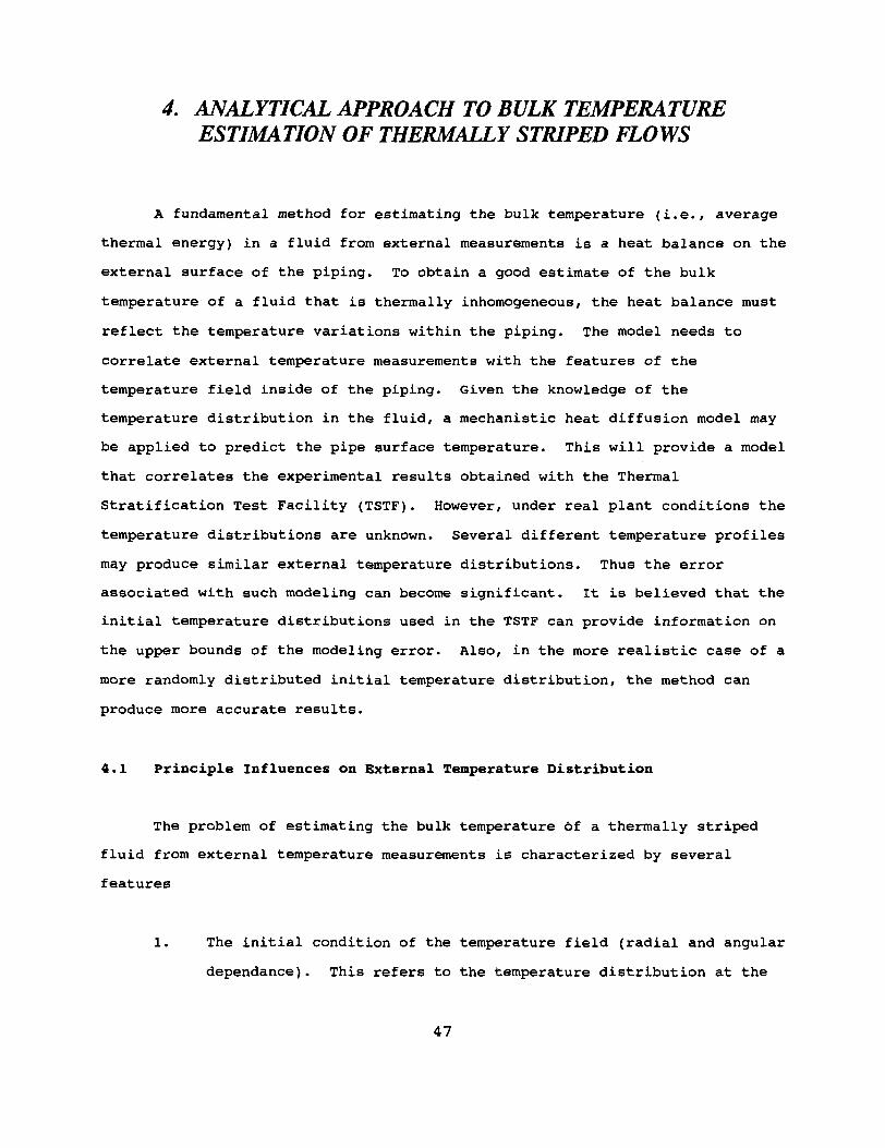
4-1 Initial Temperature Distribution for the Semi-Circular Inlet Geometry 49

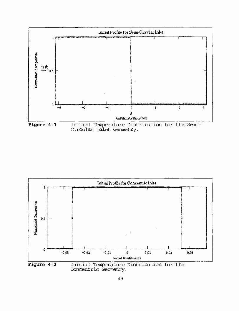
4-2 Initial Temperature Distribution for the Concentric Inlet Geometry 49

4-3 External Temperature Profile for Semi-Circular Inlet Geometry at Station HC1 54

4-4 Internal Temperature Profile for Semi-Circular Inlet Geometry at Station HC1 54

4-5 Measured Temperature Distribution (at Q=n/2) for the Semi-Circular Inlet Geometry 56

4-6 Calculated Temperature Distribution (at Q=n/2) for the Semi-Circular Inlet Geometry 56

4-7 Measured Temperature Distribution (at 0=7r/2) for the Concentric Inlet Geometry 57

4-8 Calculated Temperature Distribution (at 9=7r/2) for the Concentric Inlet Geometry 57

4-9 Eddy Diffusivity for Turbulent Pipe Flow 59 4-10 Measured External Temperature Distribution, Semi-Circular

Inlet, HC Stations 62 4-11 Calculated External Temperature Distribution, Semi-Circular

Inlet, HC Stations 62 4-12 Measured External Temperature Distribution, Concentric

Inlet, HC Stations 63 4-13 Calculated External Temperature Distribution, Concentric

Inlet, HC Stations 63

ix

LIST OF FIGURES (cont'd)

Description Page

Group Averages for Semi-Circular Inlet, HC Stations 66 Group Averages for Semi-Circular Inlet, CH Stations 66 Group Averages for Concentric Inlet, HC Stations 69 Group Averages for Concentric Inlet, CH Stations 69 Extrapolation of Group Averages for the Concentric Inlet Geometry, HC Stations 70 Extrapolation of Group Averages for the Concentric Inlet Geometry, CH Stations 70

x

EXECUTIVE SUMMARY

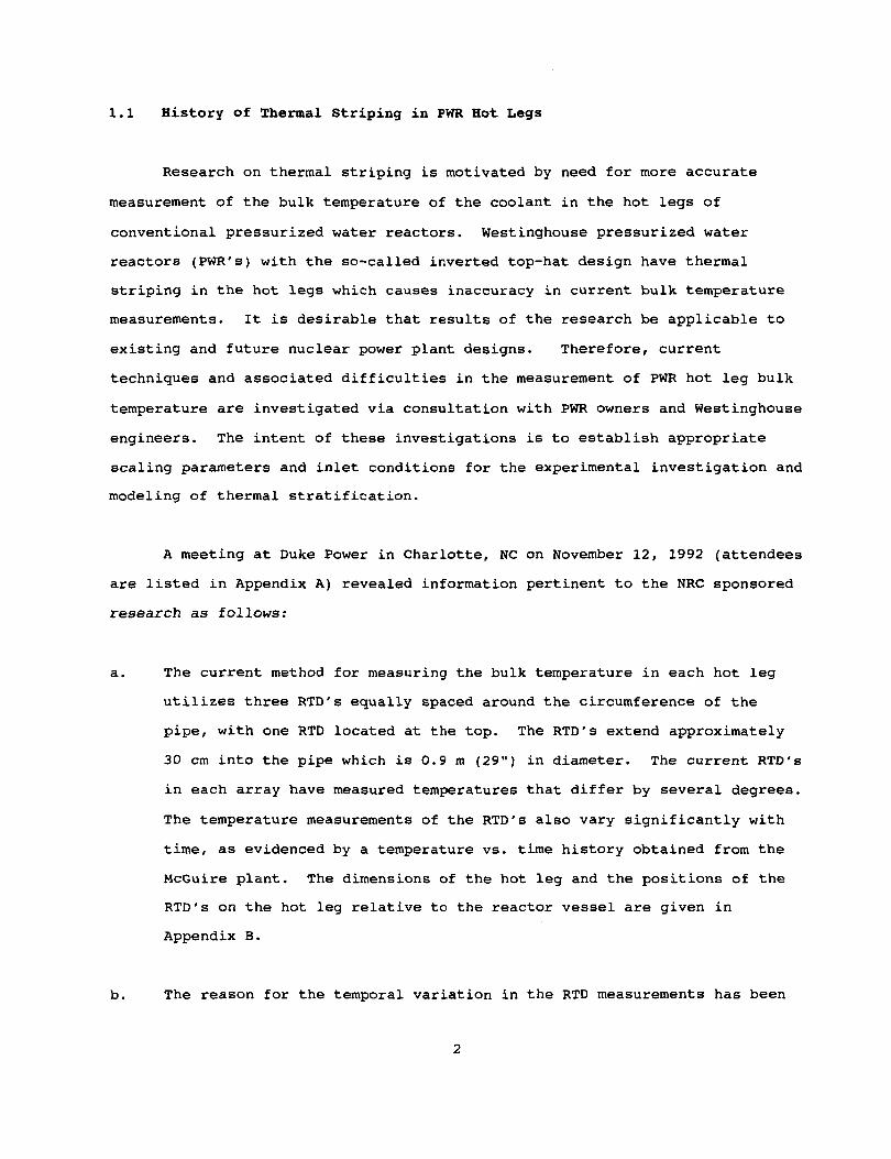
The hot leg flows in some Pressurized Water Reactor (PWR) designs have a temperature distribution across the pipe cross-section. This condition is often referred to as a thermally striped flow. This temperature distribution is known to vary with time, apparently switching between two or three relatively stable configurations. The temperature distribution in the hot legs makes the accurate measurement of the bulk temperature of the core exit flow difficult. This research investigates methods to measure the bulk temperature of a flow in a pipe using externally mounted thermocouples.

The research contains experimental and analytical components. The experimental component involves a study of thermally striped flows in a three inch inner diameter pipe with Reynolds numbers around 500,000. Three different spatial inlet temperature distributions are considered. The first inlet configuration splits the pipe cross-section into two half moons, one on the top of the pipe, the other on the bottom. The second inlet temperature distribution is a concentric annular configuration. The third inlet temperature distribution is an eccentric annular configuration. The temperature distribution in the flow downstream of the inlet is measured inside the pipe using a rake of thermocouples mounted on an aerodynamic mast. The temperature distribution on the exterior of the pipe is measured using a ring of thermocouples pressure mounted by a clamp to the exterior of the pipe. Measurements of this type are taken at several positions downstream of the inlet. The actual bulk temperature is known in all tests through measurement of the flow rate and temperature for both of the inlet streams.

The development of the temperature profile downstream of the inlet is predicted using standard models for thermal diffusivity in turbulent pipe flows. These models predict spatial temperature gradients in the flow field as a function of axial position downstream of the inlet. These models are found to predict the measured data well. This information is useful in

XI

determining the spacing of thermocouples in the internal rake and in the external ring necessary to achieve an accurate representation of the spatial temperature profile in the flow and the associated bulk temperature.

The bulk temperature is predicted from the external temperature measurements using two strategies. The first strategy uses the mean temperature value from the external values as the bulk temperature. This technique is based on the definition of the bulk temperature and assumes the pipe cross-section is divided into equal pieces, like a pie, with each piece having a temperature corresponding to the external temperature value. A uniform velocity profile is also assumed. The second strategy utilizes a Backpropagation Neural Net Algorithm to predict the bulk temperature based on the pipe external temperature measurements.

Both bulk temperature prediction strategies work well for the inlet temperature distribution where the cross-section is divided into two half moons. Unfortunately, the bulk temperature is not well predicted using the mean value strategy for the inlet configuration corresponding to concentric annuli because one of the temperature stripes is not in intimate contact with the pipe wall. The Backpropagation Neural Net Algorithm shows some advantage over the simple mean value method. However, the data gathered in the experimental part of this research are not diverse or numerous enough to properly train the network.

x n

/ . INTRODUCTION

A combined experimental and theoretical approach is employed to establish measurement strategies that allow accurate bulk temperature determination in PWR hot legs. The experimental effort uses a three inch diameter test pipe supplied with hot and cold fluid streams. The fluid streams are introduced in three different inlet geometries. The fluid flow velocities in the pipe are from 5 m/s to 8 m/s. Temperature profiles in the pipe are measured using an instrumented spool piece that could be placed at several positions downstream of the hot and cold fluid stream inlets. The spool piece is fitted with 14 thermocouples mounted circumferentialy around the exterior of the pipe. A rake of 12 thermocouples spans the flow along the vertical cross-section. The spool piece allows characterization of the centerline temperature profile in the pipe at several positions downstream of the hot and cold fluid stream inlet.

Mechanistic thermal mixing models are employed to predict the experimentally measured temperature profiles. The mixing models use existing models for mixing length in fully developed pipe flow to derive thermal diffusivity as a function of the radial position. The radially varying thermal diffusivity is then used to predict the temperature profile development in the test section. The temperature field development is thereby described as a transient conduction problem. This technique works for the portion of the flow cross-section where the time average velocity is relatively constant, which is over 90% of the pipe diameter for the highly turbulent flows (i.e., Re > 106 ) considered in this study.

1

1.1 History of Thermal Striping in PWR Hot Legs

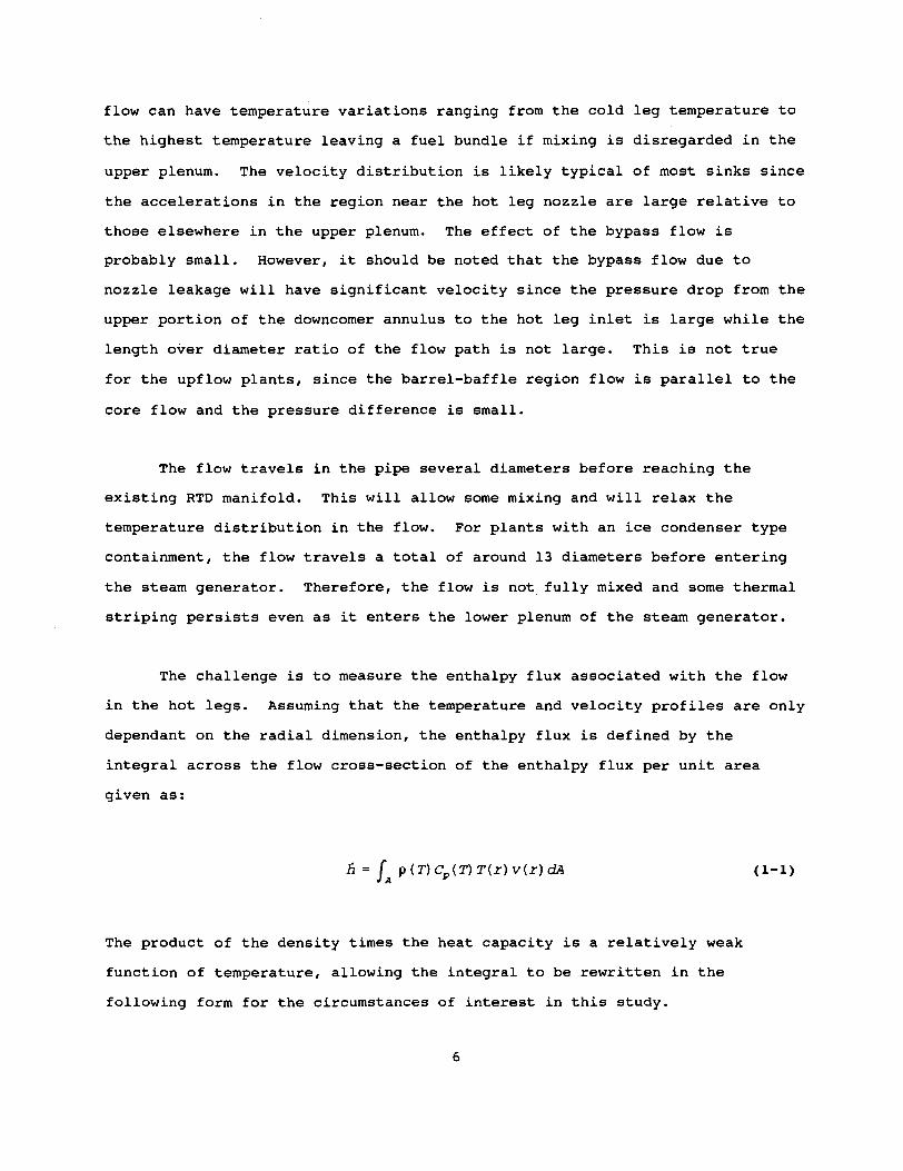
Research on thermal striping is motivated by need for more accurate measurement of the bulk temperature of the coolant in the hot legs of conventional pressurized water reactors. Westinghouse pressurized water reactors (PWR's) with the so-called inverted top-hat design have thermal striping in the hot legs which causes inaccuracy in current bulk temperature measurements. It is desirable that results of the research be applicable to existing and future nuclear power plant designs. Therefore, current techniques and associated difficulties in the measurement of PWR hot leg bulk temperature are investigated via consultation with PWR owners and Westinghouse engineers. The intent of these investigations is to establish appropriate scaling parameters and inlet conditions for the experimental investigation and modeling of thermal stratification.

A meeting at Duke Power in Charlotte, NC on November 12, 1992 (attendees are listed in Appendix A) revealed information pertinent to the NRC sponsored research as follows:

a. The current method for measuring the bulk temperature in each hot leg utilizes three RTD's equally spaced around the circumference of the pipe, with one RTD located at the top. The RTD's extend approximately 30 cm into the pipe which is 0.9 m (29") in diameter. The current RTD's in each array have measured temperatures that differ by several degrees. The temperature measurements of the RTD's also vary significantly with time, as evidenced by a temperature vs. time history obtained from the McGuire plant. The dimensions of the hot leg and the positions of the RTD's on the hot leg relative to the reactor vessel are given in Appendix B.

b. The reason for the temporal variation in the RTD measurements has been

2

attributed to the so-called Upper Plenum Anomaly. The flow pattern in the upper plenum exhibits two or more stable patterns during normal operation of the reactor. Each of these flow configurations results in a different temperature distribution measured at the RTD positions on each hot leg, and in a different bulk temperature in each hot leg. This behavior is more noticeable in low leakage cores because the spatial temperature distribution of coolant leaving the top of the core is more pronounced.

c. Westinghouse is sponsored by a sub-group of the Westinghouse owner's group called the Upper Plenum Anomaly Sub-group to evaluate the flow patterns in the upper plenum using Computational Fluid Dynamic (CFD) techniques. The list of the members of this sub-group are given in Appendix C.

Pursuant to the meeting in Charlotte, the following was learned from personal communication with Walt Lyman, a consulting Engineer in Fluid Systems Engineering at Westinghouse. Both the inlet temperature distribution and the inlet velocity distribution are currently unknown for the hot legs. Further, the CFD analysis currently underway will require a benchmark to be credible given the complexity of the flow geometry and model. The benchmark for the CFD analysis may be partially fulfilled by experiments performed in Japan.

The RTD manifold is located three to five pipe diameters away from the reactor vessel on the Watts Bar Nuclear Plant operated by TVA, which is a typical Westinghouse PWR with an ice condenser containment. This manifold replaces the RTD bypass line that was originally used in these systems, but was removed due to safety issues. The RTD bypass line was a small diameter line in parallel to the hot leg in which the RTD's were mounted. The flow in this line was well mixed and originated from a single position on the hot leg circumference. Therefore, the RTD's were exposed to a single water

3

temperature in the bypass line. Thermal striping in the hot leg may have been present, but undetected.

The true flux of enthalpy through each of the hot legs must be known in order to allow an energy balance to be performed on the primary coolant loop. This is important to allow operation of the plant at peak efficiency and is also critical to the plant safety systems. The present uncertainty in the enthalpy flux through the hot legs has caused these nuclear plants to operate at less than their potential safe power output by a few tenths of a percent.

1.2 Determination of Bulk Temperature in PWR Hot Legs

The character of the thermal striping in the hot leg should be understood in order for the measurement strategy developed herein to be useful. The nature of the thermal striping can be quantified by considering the flow in the upper plenum which provides the inlet velocity and temperature distribution to the hot legs. The flow in the upper plenum is not well quantified in any study available in the open literature. However, several general characteristics of this flow can be identified.

The source of flow in the upper plenum comes from hundreds of flow paths in the core upper tie plate. These flows have spatially varying temperatures and velocities. The temperature distribution is on average peaked in the center of the core due to low leakage fuel loading designs. The flow is also peaked in the center of the core to maintain uniform thermal margins. Thus, the source term can be globally characterized with a center peaked radial profile of a cosine shape for both temperature and velocity.

The sink for the flow in the upper plenum is three operating hot leg nozzles. Each hot leg nozzle takes approximately the same amount of flow. The variation in flow between the three hot legs depends on the configuration

4

of the plant and the condition of the individual pumps and steam generators. The reactor is fitted with four hot legs, therefore, the three operating nozzles are not located symmetrically about the centerline of the reactor vessel.

The flow into the hot legs likely has some angular momentum characteristic of sink flows. The temperature distribution at the sink inlet is a function of the temperature distribution of the source, the flow pattern from the source to the sink, and the mixing that takes place during the time the fluid travels from the source to the sink. The upper plenum has many internal structures that promote mixing of the flow as it travels from the source to the sinks.

The flow in the upper plenum has at least two "stable" flow configurations. These configurations can be thought of as local minima in the energy of the flow. Occasionally the system will move from one local minimum to another. This movement may be motivated by an external perturbation of the system, or may be motivated by a particular trajectory of the state space that occurs as a natural consequence of randomness (i.e., chaos) internal to the flow. Westinghouse sponsored experiments in Japan (Walter Lyman, 1992) and may have more quantitative information on the flow in the upper plenum.

Note also that the hot leg nozzles fitted to the inner core barrel fit loosely to the outer pressure vessel. A leakage or bypass flow from the downcomer annulus enters the hot legs. This flow is thought to be small. Also, some plant configurations allow coolant to flow up through the barrel-baffle region, by-passing the core. These flows enter the hot leg near the cold leg temperature.

This description of the flow in the upper plenum leads to some qualitative information pertaining to the flow entering the hot legs. The

5

flow can have temperature variations ranging from the cold leg temperature to the highest temperature leaving a fuel bundle if mixing is disregarded in the upper plenum. The velocity distribution is likely typical of most sinks since the accelerations in the region near the hot leg nozzle are large relative to those elsewhere in the upper plenum. The effect of the bypass flow is probably small. However, it should be noted that the bypass flow due to nozzle leakage will have significant velocity since the pressure drop from the upper portion of the downcomer annulus to the hot leg inlet is large while the length over diameter ratio of the flow path is not large. This is not true for the upflow plants, since the barrel-baffle region flow is parallel to the core flow and the pressure difference is small.

The flow travels in the pipe several diameters before reaching the existing RTD manifold. This will allow some mixing and will relax the temperature distribution in the flow. For plants with an ice condenser type containment, the flow travels a total of around 13 diameters before entering the steam generator. Therefore, the flow is not fully mixed and some thermal striping persists even as it enters the lower plenum of the steam generator.

The challenge is to measure the enthalpy flux associated with the flow in the hot legs. Assuming that the temperature and velocity profiles are only dependant on the radial dimension, the enthalpy flux is defined by the integral across the flow cross-section of the enthalpy flux per unit area given as:

A = f p(T)Cp{T)T{r)v(r)dA (1-1)

The product of the density times the heat capacity is a relatively weak function of temperature, allowing the integral to be rewritten in the following form for the circumstances of interest in this study.

6

A = 2npCp JR T{z) v{r) rdr (1-2)

The velocity distribution and the temperature distribution in the pipe cross-section must be known before the enthalpy flux can be accurately determined.

7

2. EXPERIMENT OBJECTIVES AND DESIGN

2.1 Experiment Objectives

This work studies the effect of a thermally striped flow through a pipe on the temperature measurements at the surface of the pipe. To accomplish this, the task is divided into five major objectives:

1. The delivery of a well-defined, thermally striped flow to the test section. This is implemented by using inlet transition pieces that deliver two different temperature streams to the test section with a specific geometric shape.

2. An accurate knowledge of the bulk temperature of the flow in the test section. This is determined by measuring the temperature of the source flows before mixing occurs, and the fluid flow rates from each source. These measurements are combined using the relation

<?1 + <?2

where g and T; (i=l,2) are the volumetric flow rate and the temperature of the two streams. (Note the specific heat and density are assumed equal for T, and T2. There is a difference of approximately 1% in the densities over the temperature span of interest here.)

3. Measurement of the internal temperature distribution. This helps to characterize the evolution of the temperature distribution as a function of axial position (i.e., along the pipe), and provides another measure of bulk temperature.

8

4. Measurement of the external surface temperatures. These measurements provide the "output", or response of the test section to the thermally striped flows. They would be the primary measurement parameter in a field application.

5. Correlation of the external measurements with the bulk temperature measurements. This is the main objective of the experiment. The external measurements provide information on the energy content of the pipe, and thus in many instances can be used to estimate the bulk temperature.

The physical implementation of items one through four are the subject of this section. The measurement results of the test runs are described in section 3. Methodologies to address item five are discussed in sections four and five.

2.2 Description of the Thermal Stratification Test Facility

The Thermal Stratification Test Facility (TSTF) was designed to simulate the effect of thermal striping in a coolant leg of a PWR. It consists of hot and cold water reservoirs, an inlet mixing piece, a test spool piece, piping, pumps, and instrumentation. A flow diagram of the TSTF is shown in Fig. 2-1. The system can deliver two different temperature streams at flow velocities up to 8 m/s. The University water system supplies the hot and cold water streams. Two inlet mixing pieces can be used to provide three different inlet geometries, semi-circular, concentric, and off-center. Temperature measurements are made in a test spool piece made of stainless steel, and instrumented with 16 surface (external) thermocouples and 12 internal thermocouples. A data acquisition system records the thermocouple measurements once per second.

9

*»

»

i

tr

M

W f t f l p) rt H-H) H-O D> rt p-O 3 t-3 n> w rt *) o H-H rt

Thermal Stratification Test Facility

, * - . .v . lT . - - . . . - , r^ - . - s . .Tr^v . ^ y , . . , . V ^ , . - , . . ' ^

Pump A

Pump B

System Description

Hot and Cold Water Reservoirs The water reservoirs are two 300 gallon vertical cylindrical polytanks.

These are the sources for different temperature streams in the test section. Each tank is equipped with a three inch penetration for discharge, and a 1.5 inch penetration and hose connection for water supply. The hot and cold water is supplied by the University physical plant. Temperatures vary seasonally, and are in the range of 15 - 25 °C for cold water and 40 - 50 °c for hot water. However, the differential temperatures remain at approximately 30 ±5 °C. Gate valves are located on the three inch discharge line to isolate the tanks from each other during filling.

Each tank has an independent differential pressure sensor and transmitter. The transmitters input to the data acquisition system so that the water volume vs. time can be logged, and the volumetric flow rates calculated. There is a calibrated thermocouple located in the discharge nozzle of each tank. The bulk temperature in the test section is determined using these measurements and equation 2.1. The thermocouples also provide a means of verifying that the source flows are isothermal.

Inlet Mixing Pieces The inlet mixing pieces provide the transition from two separated

isothermal flows to a single, thermally striped flow. They also provide the specific inlet geometry from which thermal mixing is allowed to proceed. In this sense, the end of the inlet mixing piece corresponds to the reactor vessel hot leg nozzle. There are two inlet mixing pieces that allow three different inlet conditions. Figure 2-2 shows the three inlet geometries, semi-circular, concentric, and off-center.

11

Inlet Geometry 1

Inlet Geometry II

Inlet Geometry III

Figure 2-2 - I n l e t Condi t ion Geometries Used In The TSTF.

12

Figure 2-3 - Inlet Mixing Piece I.

Figure 2-4 - Inlet Mixing Piece II.

13

Inlet mixing piece I provides the semi-circular inlet condition. It is constructed out of three inch, schedule 40, clear PVC. Water flows from tank A into the bottom section of the wye, and from tank B into the top portion of the wye. The flows remain separated by a divider plate located horizontally along the discharge portion of the mixing piece. At the end of the horizontal run, the flows are allowed to begin mixing. A photograph of this inlet mixing piece is shown in Figure 2-3.

Inlet mixing piece II provides the concentric and off-center inlet conditions. The horizontal run is constructed out of three inch, schedule 40, white PVC, and the wye portion is constructed out of two inch, schedule 40 PVC. The bottom leg of the wye actually penetrates the three inch section at the wye, and runs through to the end, thus keeping the flows separate until the end of the mixing piece is reached. This configuration provides the concentric inlet condition. The center tube is supported at the end by three set screws. By adjusting these set screws, the end of the inner tube can be deflected in any direction. Setting the inner tube against the inside of the outer pipe provides the off-center inlet condition. Water flows from tank A into the bottom section of the wye, and from tank B into the top portion of the wye. At the end of the horizontal run, the flows are allowed to begin mixing. A photograph of this inlet mixing piece is shown in Figure 2-4.

A convention used in this work defines the temperature configuration of the inlet as the temperature of water (i.e., H for hot and C for cold) that is flowing from tank A or from tank B. For example, the temperature configuration HC refers to hot water flowing from tank A, and cold water flowing from tank B. Temperature configuration CH refers to the opposite situation. Thus for mixing piece I, the HC configuration would allow hot water to be the bottom layer in the test spool, and cold water to be the top layer. This convention is used in the test matrix to identify all possible combination of inlet conditions and axial positions.

14

Test Spool Piece and Extension Spools The test spool piece is designed to simulate the thermal response

(scaled) of a reactor coolant system hot leg, and to provide discreet temperature measurements at points on the surface, and in the interior flow of the pipe. It is 18 inches in length, and is constructed of three inch, schedule 40 stainless steel. This schedule was chosen because the dimensions scale well to a reactor coolant pipe. The inner diameter of 3.Q68 inches and wall thickness of 0.216 inches, gives a diameter to wall thickness ratio of 14.2. By comparison, the reactor coolant pipe has a diameter (29 inches) to wall thickness (2-1/3 inches) ratio of 12.4. The pipe material (304S) also has the same thermal conductivity as the reactor coolant system piping. Flanges are welded onto each end to provide for easy installation into and removal from the TSTF. A photograph of the test spool piece is shown in Figure 2-5.

To measure the external surface temperatures, an array of type k thermocouples are attached at the midpoint of the spool piece by use of a PVC harness. This thermocouple harness contains 16 thermocouple junctions, arranged in a circle with a spacing of approximately 22.5 degrees. It is secured to the outside of the spool piece by a hose clamp to ensure that even pressure is applied to all of the thermocouples. Conductant paste is also applied to each junction to further ensure good thermal conductivity. Internal temperature measurements are made by an array of thermocouples that is inserted into the spool piece through a hole drilled at the midpoint. This thermocouple probe contains 12 thermocouples at a pitch of approximately five millimeters. Thermocouple wire is run through a hole bored down the center of a brass "mast", and the junctions emerge from a set of 12 holes drilled into the face of the mast. The crossection of the mast is shaped like an airfoil to reduce drag and the resultant perturbations of the flow. The junctions protrude approximately 6 millimeters from the surface to allow temperature measurements to be taken before the mast creates a disturbance in the flow

15

pSS'J3!M""^n"g«

*mmji 9" 0$f

„^w.

-&^^nK^

Figure 2-5 - Test Spool Piece Installed In The TSTF.

16

field. The probe mast is inserted vertically into the bottom of the pipe, and is countersunk into the top of the pipe for stability. Table 2-1 gives the positions of the thermocouples inside the pipe, and around the exterior perimeter. A photograph of thermocouple harness and probe are shown in Figures 2-6 and 2-7 respectively.

A set of extension spool pieces were made to allow the test spool piece to be moved to different axial positions. Table 2-2 shows the length of each extension spool, and the distance in inches and pipe diameters that it positions the temperature sensors on the test spool piece. The total length of the test section is 36 inches; 18 inches for the test spool piece and 18 inches for a combination of extension spool pieces.

The axial placement of the test spool piece by using the extension pieces defines the axial measurement stations that are used in the test procedures. A measurement station is defined by the combination of axial displacement of the test section, and temperature configuration of the inlet (i.e., HC or CH ). Thus if the inlet geometry I is used without an extension spool piece, and tank A contains hot water and tank B contains cold water, then the measurement station is designated as HC1-I. Changing the extension spool to number 5 would be designated as HC6-I, and so forth.

Pumps And Discharge Tank

There are two, 300 gpm capacity pumps that draw water from the tanks through the spool piece. The pumps are connected by a wye to a pipe at the end of the test spool piece. They each have a vertical discharge that turns through two elbows into a 500 gallon discharge tank. Each pump can be isolated by a quarter turn ball valve on the discharge pipe. The system can be operated with either one, or both, of the pumps. Operating with both of the pumps creates a combined flow rate of over 550 gpm (approximately 8 m/s). Single pump operation yields a flow rate of 370 gpm (approximately 5 m/s).

17

Table 2-1 - Thermocouple Positions

Internal Thermocouples Number Position from pipe bottom(mm)

Al 6 A2 12 A3 18 A4 24 A5 30 A6 36 A7 39 A8 42 A9 48 A10 54 All 60 A12 66 A13 72

External Thermocouples Number Position around pipe (degrees)

Bl 0 B2 23 B3 45 B4 68 B5 90 B6 113 B7 135 B8 158 B9 180 BIO 203 Bll 225 B12 248 B13 270 B14 293 B15 315 B16 338

18

Figure 2-6 - Thermocouple Harness.

Figure 2-7 - Thermocouple Probe.

19

Table 2-2 - Extension Spool Pieces

Spool Number Length Sensor Axial Position (in) (in) (L/Dl

1 6 15 5 2 9 18 6 3 12 21 7 4 15 24 8 5 18 27 9

Data Acquisition System The data acquisition system consists of a 48 channel A/D stand alone

unit complete with termination board, cold junction compensation, and signal conditioning software. The unit can sample up to 48 analog inputs at the rate of 1 per second. It is connected to the parallel port of an IBM-PC. The data acquisition software scales the voltages to temperatures, and writes the results to the hard disk in an ASCII format file.

A total of 29 thermocouples from the test spool (16 external, 13

internal) terminate in the data acquisition unit. There are also two thermocouples that measure the temperature of each of the supply tanks. In addition, the pressure transmitters on the supply tanks also input to the unit, providing a log of tank level vs time {i.e., flow rate). All of the data is post-processed using the spreadsheet program Excel.

2.3 System Operation

The supply tanks isolation valves are closed, and one tank is filled from the hot water supply, and the other tank from the cold water supply. During the filling process, the data acquisition system is started and the

20

proper operation of all sensors is verified. When the tank level is above the discharge of the pumps, water is allowed to enter the test leg first from one tank, then from the other (after re-isolating the first). This procedure allows the purging of as much air as possible from all of the piping, without allowing the water in the two tanks to mix. It also allows the test spool piece to come to a thermal equilibrium at a temperature somewhere between that of the two reservoirs. This helps assure the longest possible run time at steady state conditions. Due to the limited volume of the supply and discharge tanks, a maximum run time of only 60 seconds is achievable.

When both tanks are at their operating levels, the water supplies are shut off. The data acquisition system is set to acquire and write to a disk file. The power switches of the pumps are aligned so that the a single throw of the master switch will start either, or both, of the pumps. As quickly as possible both of the supply tank isolation valves are opened, followed by the appropriate pump discharge valve(s). Since there is a 1.5 foot level difference between the two supply tanks, the above steps should be performed quickly to reduce the effect of level equalization and mixing. Gravity flow of the water is allowed to occur for a few seconds to sweep each supply leg of thermally mixed water (the supply tanks are higher than the pumps). The master pump switch is then closed to start the pumps. When the discharge tank is nearly full, or either one of the supply tanks drops below 50 gallons, the master pump switch is opened, and all isolation valves re-closed. Supply tank refill can be started while the discharge tank is pumped out and the test run data is post-processed.

21

3. Experiment Results And Observations

3.1 Description of the TSTF Test Program

The test program is divided into three major sections characterized by the three inlet geometries. A full set of test runs consists of measurements taken for each temperature configuration, at each of the six axial stations. At least two test runs are made for each configuration to ensure that the conditions are repeatable. An extensive set of tests were performed for inlet geometries I and II. A less extensive set of test runs were made for inlet geometry III because of similarities that were observed between tests using inlet geometries I and III. The test program that was performed is summarized in Table 3-1.

3.2 Character i s t i c TSTF Process Conditions

Process conditions for the TSTF consist of inlet water temperatures, supply leg flow velocities, and total flow velocity. The test procedure reproduces similar process conditions for all test runs. The water supply is from the University physical plant, and therefore the maximum and minimum temperatures available varied during the study. However, within a given seasonal period, the temperatures of both hot and cold water remained very consistent.

22

Table 3-1 - Thermal Stratification Test Matrix Inlet Geometry Temperature Axial

I HC 1 Semi-circular inlet geometry, hot lower flow, cold upper flow.

I HC 2

Semi-circular inlet geometry, hot lower flow, cold upper flow.

I HC

3


I HC

4


I HC

5


I HC

6


I

CH 1 Cold lower flow, hot upper flow.

I

CH 2

Cold lower flow, hot upper flow.

I

CH

3


I

CH

4


I

CH

5


I

CH

6


II HC 1 Concentric inlet geometry, hot center flow, cold outer flow.

II HC 2

Concentric inlet geometry, hot center flow, cold outer flow.

II HC

3


II HC

4


II HC

5


II HC

6


II

CH 1 Cold center flow, hot outer flow.

II

CH 2

Cold center flow, hot outer flow.

II

CH

3


II

CH

4


II

CH

5


II

CH

6


III HC 1 Off-center inlet geometry, hot center flow, cold outer flow.

III HC 3

Off-center inlet geometry, hot center flow, cold outer flow.

III HC

4


III HC

6


23

The nominal hot water temperature is 50 "C and the nominal cold water temperature is 17 °c. The average differential temperature is approximately 33 °C. The supply leg flow velocities are a function of the number of pumps running and the type of inlet geometry used. Due to differences in the piping arrangements for each inlet condition, the flow velocities for the supply legs are not equally balanced. Table 3-2 gives the average fraction of the total flow that each supply leg contributes. The fractions are presented in percent of total flow, and in units of gallons per minute. Equal flow balance is not necessary as long as the actual flow rates are measured. Pressure transmitters tapped into the bottom of each tank measure these flow rates. For the majority of the tests run, only one pump is used, yielding a flow velocity of approximately 5 m/s. This equates to approximately 360 gpm. It was determined early in the test program that higher flow velocities did not produce any significant differences in the temperature profiles. Examples of temperature distributions using a higher flow velocity (i.e., 8 m/s) are presented later in this section.

In the reactor coolant system (RCS), the flow velocity at full power is approximately 14 m/s, which corresponds to a Reynolds number on the order of 8 x 108. At a flow rate of 5 m/s, the Reynolds number in the TSTF is approximately 5 x 10s. Thus the Reynolds number in the TSTF does not scale to

Table 3-2 - Supply Leg Flow Rate Ratios.

Inlet Geometry Percent of Total Flow Flow Rate (gpm) Semi-circular Supply Leg A: 48 173

Supply Leg B: 52 187 Concentric Supply Leg A: 60 216

Supply Leg B: 4 0 144 Off-center Supply Leg A: 60 216

Supply Leg B: 40 144

24

that of the RCS. Equality with the RCS Reynolds number is not possible in a test facility of this size without increasing the pumping capacity and tankage volume. To do so would have far exceeded the funding for equipment in this project. However, it was noted that testing at a higher Reynolds number corresponding to 8 m/s did not produce any appreciable change in the character of the measured temperature distributions.

3.3 Description of the Experimental Results

The results of measurements made with the TSTF are presented in the following sections. Results are categorized by the type of inlet geometry used. Graphical presentation of the data is prepared using time-averaged values of the steady state portion of each group of test runs. The sample size used for the time-averages is typically about 30 (i.e., 30 seconds). Recall that the internal temperatures are measured vertically across the center of the pipe. Thus the mean internal temperature measurements present a distribution perpendicular to the centerline of the pipe. The external measurements present an angular temperature distribution around the external perimeter of the pipe. Note that all of the temperatures are normalized using the expression

T -T T* = m c 3-1

where Th and Tc are the hot and cold temperature measurements taken at the tank outlet, and T m is the measured temperature at the probe.

Standard deviations for each set of measurements are also presented. These plots indicate the areas of maximum temperature variance. For the internal measurements, this indicates the regions in the vicinity of the sensors where the highest degree of thermal mixing is occurring. In the case

25

of the external measurement, the standard deviation is an indication of thermal mixing near the inside surface of the pipe, or possibly transient conduction in the pipe wall.

Two sets of internal and external measurements are made at each axial location, one set for the HC temperature configuration, and one set for the CH temperature configuration. Measurements are taken at six axial locations (e.g., HC1 through HC6) at distances from the inlet mixing piece of 9, 15, 18, 21, 24, and 27 inches (corresponding to an L/D of 3, 5, 6, 7, 8, and 9 respectively).

Inlet Geometry I - Semi-Circular Inlet The inlet condition for this geometry allows water from tank A to enter

the bottom semi-circle and water from tank B to enter the top semi-circle. Thus all test runs using the HC designation have hot water in the bottom half of the semi-circle, and cold water in the top half. Test runs with the CH designation represent the opposite case.

The results of the inlet geometry I tests are presented in Figures 3-1 through 3-8. Figure 3-1 shows the mean internal temperature profile at each measurement station. Note the s-shaped curve for station HC1. As expected, the streams are still largely separated, with the largest thermal gradient in the center region of the pipe. Progressing down the pipe, the profile almost becomes linear, indicating a nearly constant temperature gradient. The external temperatures are shown in a contour plot in Figure 3-2. The overall pattern shows the temperature gradient matching the internal distribution (i.e., cold on the upper half of the pipe and hot on the lower half of the pipe). Moving clockwise, it can be seen that the maximum thermal gradients for HC1 appear in the regions between 338° and 23°, and between 180° and 225°, corresponding to positions near the horizontal plane of the pipe. As the axial distance from the inlet is increased, the temperature gradient increases

26

1 -r 0.9-

QJ

S 0.8-1 0.7-DJ

| . 0.6 -!» 0.5 -•B 0 . 4 -01

JH 0.3-1 0.2-| 0.1 -

0--0.1

Semi-Circular Inlet - Internal Temperatures (HC)

10 20 30 40 50 60 Distance horn bottom of pipe (mm]

— i —

70 —i

80

Figure 3-1 - In ternal Temperatures For In le t Geometry No. 1, HC Stat ions .

Semi-Circular In le t - External Tempera tu res (HC)

•HC6

c s i C M c x i c j c u m m c n

Angular Position (clockwise)

• 0-0.1 3 0.1-0.2 • 0.2-0.3 • 0.3-0.4 • 0.4-0.5 D 0.5-0.6 • 0.6-0.7 H 0.7-0.8 • 0.8-0.3 • 0.9-1

Figure 3-2 - External Temperatures,For Inlet Geometry No. 1, HC Stations. 27

in the clockwise direction until, for HC6, it spans the region from 180° to 270°. This indicates a cooling of one of the bottom quadrants of the pipe, which can also be seen in Figure 3-1. A less pronounced warming of the upper quadrant (centered about 23°) is also visible, and also corresponds to Figure 3-1. Thus the external temperature distribution reflects some of the structures of the internal temperature field. This demonstrates that the thermal striping induced by this inlet geometry can be detected by external measurements.

Ideally, the maximum thermal gradients should appear centered on the horizontal plane of the pipe. Note however that the temperature profiles are slightly rotated in the clockwise direction. This is attributed to the effects of possible circulation caused by bends in the flow within each inlet leg. This could also be attributed to the slight difference in the hot and cold flow rates. The apparent clockwise "rotation" of the external temperature distribution as the flow progresses downstream may indicate this effect. Recall that station HC1 is located nine inches (three pipe diameters) downstream of the inlet mixing piece, thus allowing this circulation to progress to the point shown in Figure 3-2 for station HC1. Due to the physical constraints of the inlet mixing piece, the external profile at the exit of the mixing piece is (within fabrication uncertainties) exactly symmetric with respect to the vertical plane of the pipe.

The standard deviations of the internal measurements are shown in Figures 3-3. The arrow shown in Figure 3-3 marks the location of the divider plate. As expected, the largest temperature variance occurs down the centerline of the pipe, corresponding to a position downstream of the divider plate. As the flow progresses axially, the magnitude of the variances increase and spread to the top and bottom of the pipe. The centerline variances appear to peak around station HC3 and then begin to decline. However, there may be additional phenomenon occurring beyond the axial

28

B 5-6

• 4-5

• 3-4

• 2-3

H 1-2

• 0-1

Internal Probe Standard Deviations (Inlet Geometry I - HC)

24 30 36 ^42 4% 54 Distance from bottom of pipe (mm)

Figure 3-3 In t e rna l Standard Deviations, Semi-Circular I n l e t , HC S ta t i ons .

• 0.8-1

• 0.6-0.8

• 0.4-0.6

H 0.2-0.4

• 0-0.2

External Probe Standard Deviations (Inlet Geometry l-HC)

r M^

HC6

•HC5

HC4 EL

f HC3 %

HC2 §

<=> LO LO LO CNI " ^ CM

^ : <y> T -co T —

L o a o c s r o L o o D c a n L o c o c s n i - o a o c 3 C M T r * - a 3 T — n co i— i— i— C N I C M C M C M C a C O O - J C n

HC1

Angular Position (degrees)

Figure 3-4 External Standard Deviations, Semi-Circular Inlet, HC Stations. 29

measurement zone that cannot be seen here.

Figure 3-4 shows the standard deviations of the external measurements. The regions of maximum variance occur near the angular positions of 0° and 200°. A large zone from 23° to 180° (i.e., the top half of the pipe) shows very little relative mixing, which corresponds to the same zone in Figure 3-2. The magnitudes of the temperature variances in the bottom portion of the pipe are generally higher than the top half of the pipe (again, corresponding to Figure 3-2). The external variations thus provide an indication of regions of temperature mixing at least along the inside wall of the pipe.

The results for the CH temperature configurations (cold water in the bottom, hot water in the top) are presented in Figures 3-5 through 3-8.

Figure 3-5 shows the mean internal temperature profile at each measurement station. By comparison with Figure 3-1, it can be seen that the CH internal profiles are the mirror image of the HC internal profiles. The observations made for the HC measurements also apply to the CH measurements. The external temperatures are shown in a contour plot in Figure 3-6. Again, the profiles for the CH configuration nearly mirror the profiles for the HC configuration. As with the HC measurements, the overall pattern shows the temperature gradient matching the internal distribution (i.e., hot on the upper half of the pipe and cold on the lower half of the pipe). Moving clockwise, it can be seen that the maximum thermal gradients for CHI appear in the regions between 338° and 45°, and between 158° and 225°, again corresponding to positions near the horizontal plane of the pipe. This is a slightly broader angular region over which the thermal gradients are large. As the axial distance from the inlet is increased, the temperature gradient increases in the clockwise direction until, for HC6, it spans the region from 158° to 270°. This indicates a warming of one of the bottom quadrants of the pipe, which can also be seen in Figure 3-5. A less pronounced cooling of the upper quadrant (centered about 23°) is also visible, and also corresponds to Figure 3-5.

30

1 T

§ 0.8 +

g. 0-6 4-E CD

I - QA 0) M

o Z 0 •-

-0.2

Semi-Circular Inlet- Internal Temperatures (CH)

10 20 30 40 50 60 Distance from bottom of pipe (mm)

CH6

70 80

Figure 3-5 In t e rna l Temperatures for Semi-Circular I n l e t , CH S t a t i ons .

Semi-Circular Inlet - External Temperatures (CH)

VI If 111 Um

l O L O L n a d L n a o o c o L n c o o n L D c o

CH6

CH5S

CM CM

en i— n LO oo CM T - r»- co r - n co T— T— T— i— c M C - a c s i c - a i N i r o n n i


10-0.1 B 0.1-0.2 • 0.2-0.3 D 0.3-0.4 • 0.4-0.5 D 0.5-0.6 • 0.6-0.7 B 0.7-0.8 • 0.8-0.3 D 0.9-1

Figure 3-6 External Temperatures for Semi-Circular Inlet, CH Stations.

31

Note that the same clockwise "rotation" that is observed in Figure 3-2 is also present here, indicating that this rotation is not attributable to thermal or buoyancy effects.

The standard deviations of the internal measurements are shown in Figures 3-7. Comparison to Figure 3-3 shows that the variance patterns are very similar. Again, the largest temperature variance occurs down the centerline of the pipe, corresponding to a position downstream of the divider plate. As the flow progresses axially, the magnitude of the variances increase and spread to the top and bottom of the pipe. Figure 3-8 shows the standard deviations of the external measurements. The regions of maximum variance match very closely to those for the HC measurements. The regions of maximum variance occur near the angular positions of 0° and 200°. However, the large zone of little relative mixing shown on the top of the pipe in the HC case is now located on the bottom of the pipe in the CH case. As in the HC case, the magnitudes of the temperature variances in the bottom portion of the pipe are generally higher than the top half of the pipe.

It should be noted that the magnitudes of the external temperature variances are an order of magnitude smaller than the internal measurement variances. In addition, the standard deviations of the sensors is on the order of 0.05 °C, with a corresponding 95% confidence interval of 0.15 °C. Thus the lower end of the magnitude scale for the measured external temperature variations is on the order of the characteristic sensor variation. While no useful information can be obtained from the lower temperature variation region, it does provide a measure for an upper bound of temperature variations in these zones. The higher magnitude temperature variations still provide useful information. If these measurements are used quantitatively, they should be corrected to account for the variation inherent in the sensors.

32

• 5-6

• 4-5

D3-4

• 2-3

H1-2

• 0-1

Internal Probe Standard Deviations (Inlet Geometry I - CH)

-CH6

18 24 30 36 4d2 48 54 Distance from bottom of pipe (mm)

Figure 3-7 Internal Standard Deviations, Semi-Circular In le t , CH Stations.

• 0.8-1

• 0.6-0.8

• 0.4-0.6

H 0.2-0.4

• 0-0.2

External Probe Standard Deviations (Inlet Geometry l-CH)

LO LO LO «\i "*" i< CM CO

CD CO Lf> OO CD CD i— CO LO CO C D L O C O O n L O C O _ C D C M T r ^ c n T — rr> co C M C M O J c s i o j n c o n

CH1


Figure 3-8 External Standard Deviations, Semi-Circular Inlet, CH Stations. 33

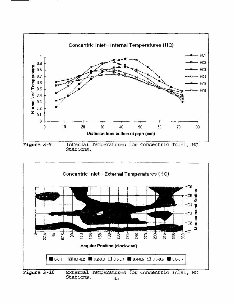
3.3.2 Inlet Geometry II - Concentric Inlet The inlet condition for this geometry allows water from tank A to enter

the center region of the pipe and water from tank B to enter the annular region of the pipe. Thus all test runs using the HC designation have hot water in the center region of the pipe, and cold water in the annular region of the pipe. Test runs with the CH designation represent the opposite case.

The results of the inlet geometry I tests are presented in Figures 3-9 through 3-16. Figure 3-9 shows the mean internal temperature profile at each measurement station. Note the bell-shaped curve for station HC1. As expected, the temperature profile is maximum near the pipe centerline, decreasing radially through the annular region to the pipe walls. Progressing down the pipe, the profile becomes flatter, indicating a decreasing temperature gradient. The external temperatures are shown in a contour plot in Figure 3-10. The overall pattern shows that the temperature gradient is roughly constant with respect to the angular dimension. Cold water flowing in the annular region dominates the temperature distribution around the pipe perimeter. The temperature of the inner core of hotter liquid is "masked" by the colder liquid in the annular region. Thus it is not possible to obtain an accurate measure of the bulk temperature of the whole stream.

As the axial distance is increased, the external temperature distribution tends toward a higher temperature. The changing profile in the axial direction provides some indication that there are temperature gradients in the fluid. The external temperatures approaches a normalized temperature of 0.6 for HC5 and HC6 in the 180° to 270° quadrant. The normalized value of the bulk temperature for this inlet geometry is also approximately 0.6. Thus there is some indication that axially spaced sensors may allow a bulk temperature estimate to be extrapolated. However, this would require a sufficient degree of thermal mixing in the radial direction to allow the center core flow to penetrate the annular layer.

34

Concentric In let- Internal Temperatures (HC)

1 T

. ° 9 -3 0.8 -cd o 0-7 + Q. E 0.6 ••

H 0.5 | 0.4 "5 0.3 + £ 5 0.2 -f

Z 0.1 0

10 20 30 40 50 60

Distance from bottom of pipe (mm) 70 80

Figure 3-9 In t e rna l Temperatures for Concentric I n l e t , HC S t a t i ons .

Concentric In let- External Temperatures (HC)

•fcpwa ' i b ^ i l L O L O L T J C D n L O O O C D ^ J - S T p ^ C O r — C D m C O CM UD -i— i— T— r—

o o L n c o o c o L n c o c j C D C M ^ T I ^ - C O T — r o t o c s j c s j c s i c s j c v j c n c n n

HC2 0 3

HC1


0-0.1 0.1-0.2 • 0.2-0.3 • 0.3-0.4 • 0.4-0.5 H 0.5-0.6 • 0.6-0.7

Figure 3-10 External Temperatures for Concentric Inlet, HC Stations. -*c

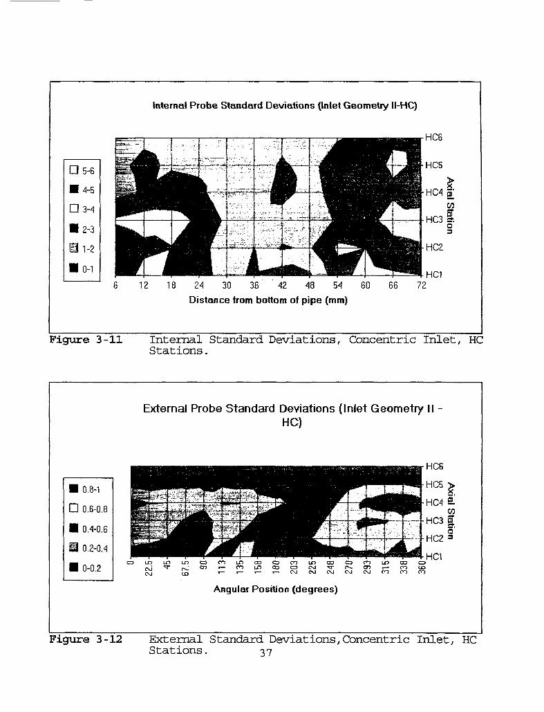
The standard deviations of the internal measurements are shown in Figure 3-11. The arrows shown in Figure 3-11 mark the location of the inner pipe wall. As expected, the largest temperature variances occur at a position corresponding to the walls of the inner pipe. At station HC1, there is a region of low variance that corresponds to the centerline of the inner pipe. As the flow progresses axially, the magnitude of the variances downstream of the inner pipe walls decline slightly. The core flow variances also increase slightly, but remain largely undisturbed throughout the remainder of the measurement stations.

Figure 3-12 shows the standard deviations of the external measurements. The region of maximum variance occur near the angular position of 0°. Maximum temperature variances occur at station HC4, and quickly drop down to the sensor variance range for stations beyond HC4. There is no well defined pattern that indicates the nature of the internal temperature distribution. Thus for this geometry, the external variations do not provide a good indication of regions of temperature mixing inside of the pipe.

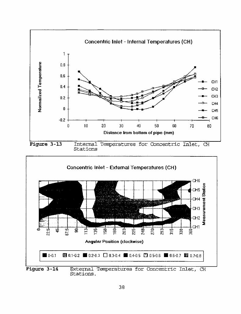
The results for the CH temperature configurations (cold water in the core region, hot water in the annular region) are presented in Figures 3-13 through 3-16. Figure 3-13 shows the mean internal temperature profile at each measurement station. By comparison with Figure 3-9, it can be seen that the CH internal profiles are the mirror image of the HC internal profiles. The observations made for the HC measurements also apply to the CH measurements. The external temperatures are shown in a contour plot in Figure 3-14. Nearly the same pattern seen in the HC measurements is repeated here, but in reverse order. Again, the overall pattern shows that the temperature gradient is roughly constant with respect to the angular dimension. Hot water flowing in the annular region dominates the temperature distribution around the pipe perimeter. The temperature of the inner core of colder liquid is "masked" by the hotter liquid in the annular region. Thus it is not possible to obtain an

36

a 5-6

• 4-5

a 3-4

• 2-3

H 1-2

• 0-1

Internal Probe Standard Deviations (Inlet Geometry ll-HC)

HC6

12 18 24 30 36 42 48 54 60 66 Distance from bottom of pipe (mm)

Figure 3-11 In t e rna l Standard Deviations, Concentric I n l e t , HC S t a t i ons .

• 0.8-1

• 0.6-0.8

• 0.4-0.6

B 0.2-0.4

• 0-0.2

External Probe Standard Deviations (Inlet Geometry II -HC)

CM CM

c o L r > a o o r « - > L O o o c 3 C O t f } a o c z > T— C O L O C O C D C M T r H . C T ) T — C O C O r— T— 7— r— C M C M C M C M C M C O O O O O


Figure 3-12 External Standard Deviations,Concentric Inlet, HC Stations. 37

Concentric Inlet- Internal Temperatures (CH)

0) w a 13 0) Q.

s <D H T3 0) '5 S w O Z

1 T

0.8

0.6 --

0.4 -•

0.2

0 +

-0.2 "1

CH1

CH2

CH3

CH4

CH5

CHG

0 10 20 30 40 50 60

Distance from bottom of pipe (mm) 70 80

Internal Temperatures for Concentric Inlet, CH Stations Figure 3-13

Concentr ic I n l e t - External Temperatures (CH)

CH6

O L O L O L o o r o L D C o o f O L n o s a c n L n o o o 07 i— en i n ao CNJ 'vT r». <T> i — CO CO

C M O J C M c s i c N j r o r o r o


0-0.1 0.1-0.2 • 0.2-0.3 • 0.3-0.4 • 0.4-0.5 H 0.5-0.6 • 0.6-0.7 H 0.7-0.8

Figure 3-14 External Temperatures for Concentric Inlet, CH Stations.

38

accurate measure of the bulk temperature of the whole stream.

As the axial distance is increased, the temperature distribution tends toward a lower temperature. The external temperatures approaches a normalized temperature of 0.4 for HC5 and HC6 in the 180° to 270° quadrant. The normalized value of the bulk temperature for this inlet geometry is also approximately 0.4. Thus, as in the HC measurements, there is some indication that axially spaced sensors may allow a bulk temperature estimate to be extrapolated.

The standard deviations of the internal measurements are shown in Figure 3-15. The pattern matches the HC measurements (Figure 3-11) very closely. Figure 3-16 shows the standard deviations of the external measurements. Again, there is no well defined pattern that indicates the nature of the internal temperature distribution. Thus for this geometry, the external variations do not provide a good indication of regions of temperature mixing inside of the pipe.

3.3.3 Inlet Geometry III - Off-Center Inlet

The inlet condition for this geometry allows water from tank A to enter a circular region that is tangent to the inside bottom of the pipe (see Figure 2-2). Water from tank B to enters the remaining area of the pipe, dominating in the upper region. Thus all test runs using the HC designation have hot water in the off-set region of the pipe, and cold water in the remaining region of the pipe. For this inlet geometry, measurements were taken at four of the HC stations (HC1, HC3, HC4, HC6). No CH measurements were performed.

39

• 5-6

• 4-5

• 3-4

• 2-3

fag 1-2

• 0-1

Internal Probe Standard Deviations (Inlet Geometry ll-CH)


CH6

Figure 3-15 Internal Standard Deviations, Concentric Inlet, CH Stations.

• 0.8-1

• 0.6-0.8

• 0.4-0.6

H 0.2-0.4

• 0-0.2

External Probe Standard Deviations (Inlet Geometry II CH)

rCH6 CH5

CM CM

LO LO

to

O Q L n a o o m L n o o o m L n o o r— c « - ) L o o o c 3 C M v r r v . c r ) T — n t o T — T — i— i — C M C M C M C M C M C O C D O O

-CH4 B. 52

•CH3 & 5"

•CH2 3

•CH1


Figure 3-16 External Standard Deviations, Concentric Inlet, CH Stations.

40

The results of the inlet geometry III tests are presented in Figures 3-17 through 3-20. Figure 3-17 shows the mean internal temperature profile at each measurement station. In the bottom half of the pipe, the hot water stream dominates the temperature distribution, reaching a maximum for HC1 at about 30 mm. As the flow progresses axially, it can be seen that the temperature gradients become flatter. The profile for HC6 actually begins to increase toward the top wall of the pipe. There is evidently a flow pattern of hotter water circulating toward the top, but not near the internal probe. This may be caused by the flow rate through the inner pipe being larger than the flow rate in the outer pipe region.

The external temperatures are shown in a contour plot in Figure 3-18. The overall pattern shows a the temperature distribution similar to that of inlet geometry I cases. However, the temperature gradients are much larger in the top half of the pipe (particularly in the first quadrant) than in the bottom half. Moving down the pipe to HC6, the temperature profile shows a large warming trend in the first quadrant (from 0° to 90°). This supports the notion of a hot flow circulating to the top of the pipe that is not detected by the internal probe (i.e., the flow followed the contour of the pipe wall in the first quadrant).

The standard deviations of the internal measurements are shown in Figures 3-19. The most distinct feature here is the region of lower thermal mixing in the bottom of the pipe. This reflects a core of hotter fluid from the inner pipe that is relatively stable, corresponding to the bottom half of the pipe shown in Figure 3-18. The intensity of the thermal mixing increases toward the top of the pipe, with the maximum shown at stations HC5 and HC6. Figure 3-20 shows the standard deviations of the external measurements. The regions of maximum variance are in the first quadrant, match very well to the temperature gradients shown in Figure 3-18. As for inlet geometry I, the external variations thus provide an indication of regions of temperature

41

Off-Center Inlet- Internal Temperatures (HC)


1 1 •— - H C 1

0 9 • ^ ^ : « ^ ^ j L ' " " "*•**. u p T » u " 3 ^ssgs'-i'E _^^ ^'^^-v^ ^ * n>—J

3 0-8- °~ ^ ^ ^ - O ^ ^ L % , X . 2 5J 0.7 • "^kC:^- ^X. "X HCb

a. £ 0.6 -.<» 1- 0.5 -•o S o.4 • 13 0.3 -£ 5 0.2 -

\ \ \ —°~ - H C 6 a. £ 0.6 -.<» 1- 0.5 -•o S o.4 • 13 0.3 -£ 5 0.2 -: ^ S ' ^ C ^

2 0.1 - ^ " ^ ^ 0 - 1 1 1 1 1 1 1 1

70 80

Figure 3-17 In t e rna l Temperatures for Off-Center I n l e t , Selected HC S ta t i ons .

Off-Center Inlet- External Temperatures (HC)

HC6

-HC5 1 S 5 .2

-HC3

IHC1

513 0) X

c \ i C M C \ j c \ j c \ j m m n


10-0.1 • 0.1-0.2 •0.2-0.3 • 0.3-0.4 •0.4-0.5 0 0.5-0.G • 0.6-0.7 H 0.7-0.8

I 0.8-0.9 Q 0.9-1

Figure 3-18 External Temperatures for Off-Center inlet, Selected HC Stations.

42

n 5-6

• AS

• 3-4

• 2-3

a 1-2

• 0-1

Internal Probe Standard Deviation (Inlet Geometry III - HC)

•r F i ^m Im. JUL.

12 18 24 30 36 42 48 Distance from bottom of pipe (mm)

54 f 6D t

•HC6

-HC5 m" CO

-HC3 I o

•HC1 66 72

Figure 3-19 In t e rna l Standard Deviations, Off-Center I n l e t , Selected HC S ta t ions .

• 0.8-1

• 0.6-0.8

• 0.4-0.6

Wm 0.2-0.4

m 0-0.2

External Probe Standard Deviations (Inlet Geometry III - HC)

ID ID ID CM CM CD

CD cn

uo oo o en en I D oo o 7 — 7— T— C M

I D CM CM

o CM

•HC6

•HC5 | j

HC3 5" i .

-HC1 en I D ao cz> er> r— en ca CM ro en en


Figure 3-20 External Standard Deviations, Off-Center Inlet, Selected HC Stations.

43

mixing along the inside wall of the pipe.

Effect Of Higher Flow Rate

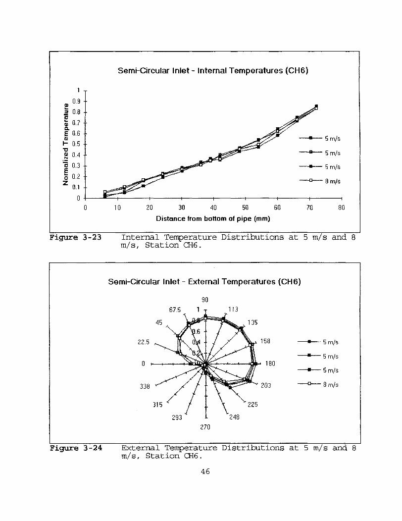
Figures 3-21 through 3-24 demonstrate the difference in the temperature distributions at the higher flow rate of 8 m/s at stations CHI and CH6. Stations CHI and CH6 were chosen to demonstrate this because they are the endpoints of the (axial) test zones, and bound the conditions throughout the test zone. The measured internal and external temperature distributions show no significant differences from the test runs with flow velocities of 5 m/s. For this reason, and to increase the test run time, it was decided to perform all remaining tests at 5 m/s. Note that these results indicate the flow development length, or length/diameter ratio, is more important than the transient time for Reynolds numbers in the 105-106 range, the increased mixing due to increased turbulence compensates for shorter residence times as the Reynold's number is increased.

44

1 T

0.9 -•

0.8 -•

0.7 -

0.6 --

w 3 13 a) a £ a 0.5 4-

•o a) M

"5 o Z

0.4 --0.3 --

0.2 --

0.1 --

0 -• -0.1

Semi-Circular Inlet- Internal Temperatures (CH1)

0 10 20 30 40 50 60

D is tance f rom bot tom of p ipe (mm)

5 m/s

5 m/s

8 m/s

70 80

Figure 3-21 Internal Temperature Distributions at 5 m/s and 8 m/s, Station CHI.

Figure 3-22

Semi-Circular Inlet- External Temperatures (CHI)

90 67.5 1 j L 113

4 5 \„J^k' ' ^ N w 1 3 5

^ K \ 6 " 22.5 ,. V \ m -

0 , — , — , — i ^ w i

• / / v * 1 5 8

••• 5 m/s

5 m/s

22.5 ,. V \ m -

0 , — , — , — i ^ w i K^J^J^-1—' 180 ®—

••• 5 m/s

5 m/s

338 " ^ / i ' - \ \ < ^ ^ 203 8 m/s

315 ^ I . . \ 225

1 293 J

L 248 270

External Temperature Distributions at 5 m/s and 8 m/s, Station CHI.

45

1 T

. 0-9 -3 0.8 -• B o 0-7 + a £ 0.6 | a>

I - 0.5 | 0.4 TB 0.3 --o 0.2 --

Z0.1 + 0

Semi-Circular Inlet- Internal Temperatures (CH6)


70 80

Figure 3-23 Internal Temperature Distributions at 5 m/s and 8 m/s, Station CH6.

Semi-Circular Inlet- External Temperatures (CH6)

90 67.5 1 j 113

45 J r * - ^ r 5 1 ^ * 1 3 5

22.5 ,. Trx ' -M • / y ^&. 1 qo _ 22.5 ,. Trx ' -M • 5 m/s

Q , , t inailS C " ' ' 'oP-' 180 5 m/s

5 m/s

5 m/s

5 m/s

5 m/s

5 m/s

338 ^ yT f • • ^ ^ S S ^ * 1 ^ 203 °— - 8 m/s

3 1 5 / . \ 225

293 248 270

Figure 3-24 External Temperature Distributions at 5 m/s and 8 m/s, Station CH6

46

4. ANALYTICAL APPROACH TO BULK TEMPERATURE ESTIMATION OF THERMALLY STRIPED FLOWS

A fundamental method for estimating the bulk temperature {i.e., average thermal energy) in a fluid from external measurements is a heat balance on the external surface of the piping. To obtain a good estimate of the bulk temperature of a fluid that is thermally inhomogeneous, the heat balance must reflect the temperature variations within the piping. The model needs to correlate external temperature measurements with the features of the temperature field inside of the piping. Given the knowledge of the temperature distribution in the fluid, a mechanistic heat diffusion model may be applied to predict the pipe surface temperature. This will provide a model that correlates the experimental results obtained with the Thermal Stratification Test Facility (TSTF). However, under real plant conditions the temperature distributions are unknown. Several different temperature profiles may produce similar external temperature distributions. Thus the error associated with such modeling can become significant. It is believed that the initial temperature distributions used in the TSTF can provide information on the upper bounds of the modeling error. Also, in the more realistic case of a more randomly distributed initial temperature distribution, the method can produce more accurate results.

4.1 Principle Influences on External Temperature Distribution

The problem of estimating the bulk temperature of a thermally striped fluid from external temperature measurements is characterized by several features

1. The initial condition of the temperature field (radial and angular dependance). This refers to the temperature distribution at the

47

inlet of the piping. The angular shape of the external temperature distribution as well as the ability to detect temperature features inside the fluid is influenced by the inlet conditions.

2. Intensity of turbulence. A higher intensity of turbulence will promote thermal mixing (i.e., thermal diffusion). Note that for flows with a high axial velocity, thermal diffusion due to turbulence is the principle mechanism for heat transport in the radial direction.

3. Convective heat transfer coefficient. The convective heat transfer coefficient (along with the temperature difference between the pipe wall and the fluid) will control the rate of heat flow from the fluid to the inner pipe wall. This element is not expected to have a significant effect.

In the TSTF, the initial temperature distributions are specified by the inlet geometries described in section 2.2. The inlet geometries were chosen to provide two extremes in the initial temperature field (semi-circular and concentric). The third geometry (off-center concentric) provides a compromise between these two extremes. The initial temperature field for the semicircular geometry (shown in Figure 4-1) has a step profile with respect to the angular dimension. In the case of the concentric geometry (Figure 4-2), it also has a square wave profile, but with respect to the radial dimension instead. It has no angular dependence.

The affect of turbulence is incorporated into the model in the form of a turbulent thermal diffusivity (see Appendix D). The high Reynold's number of the flow indicates that the axial momentum flux is much greater than any radial momentum flux. Thus the primary means of heat transport in the radial

48

Initial Profile for Setni-Ckcular Inlet 1 i l l

s |

i

' 1(6) ;i

1 I ! - 3 - 2 - 1 0 1 2 3

0 Anguki Position (rad)

Figure 4-1 Initial Temperature Distribution for the Semi-Circular Inlet Geometry.

Initial Profile for Concentric Inlet

! AH

|

i

1

• 0.3

1

I

1 i

1 l I 1

i

1

i

1 0

-0.03 -0.02 -0.01 0 0.01 RadM Position (m)

0.02 0.03

Figure 4-2 Initial Temperature Distribution for the Concentric Geometry.

49

direction is turbulent thermal diffusion. The TSTF was not designed to acquire data on turbulent fluctuations. Thus the total thermal diffusivity is modeled using conventional methods as outlined in Appendix D.

The convective heat transfer coefficient is calculated using the Dittus-Boelter correlation for the Nuselt number. It is also estimated from the transient portion of the TSTF test data as an independent check of the Dittus-Boelter correlation results.

4.2 Internal Temperature Distributions

In the TSTF, internal temperature measurements are taken across the flow along the vertical axis of the pipe cross-section. This axis is used because it is symmetric with respect to the angular dimension for the semi-circular inlet condition and for the concentric inlet condition (which ideally has no angular dependance). These measurements provide a good indication of the temperature distribution down the center of the pipe cross-section. They can be used to directly calculate the bulk temperature of the fluid, and to help validate the model predictions. The temperature profiles for all of the test runs are presented in Chapter 3.

4.2.1 Temperature Distribution for the Concentric Inlet Condition

We will first solve the heat diffusion equation for this geometry since it is the easier case. The time-dependant heat diffusion equation in circular cylindrical coordinates with constant fluid properties and no internal heat source is given by

x dr\ drj r 2 QQ2 dz2 a dt

50

where a is the effective thermal diffusivity of the fluid given by

« = -prz + «turi> 4-2

where a^ is the effective thermal diffusivity due to turbulence. For the concentric case, it is assumed that T is a function of r and t only.

1 9 /_ dT\ _ 1 BT A , 1 Mte) ~~i~5i 4 " 3

This expression of the heat diffusion equation follows a disk of fluid moving at the mean velocity (V) of the fluid. Thus the axial position of the fluid can be related to the time variable by t=z/V. The solution of this equation is expressed as

T(z,t) = (AJ0(Xr) + BY0(\r))e-**-2t + C 4-4

where A is a separation constant and A, B, and C are integration constants. The constant C allows for a non-zero steady state solution as t -» °o. For the two temperature region case, this would be the bulk temperature as given by

T = _l_i L_2 4-5 W

where W, and W2 are the volumetric flow rates for temperature region 1 and temperature region 2, and W is the total flow rate. This expression assumes that the product of density and heat capacity are equal for temperature

51

regions 1 and 2. To simplify the analysis, it is assumed that the pipe surface is perfectly insulated (adiabatic boundary condition), and that the volumetric flow rates of both temperature streams are equal. Thus the constant C is equal to a normalized mean temperature, 0.5. The condition that T(r,t) remain finite as r approaches zero requires that B equal zero. The boundary condition at r=0 (i.e., the normalized value of T at r=0 is one) also requires the constant A to be set equal to 0.5.

A slightly different approach is used to determine the value of the separation constant X. Normally in a problem like this, the value of the separation constant is obtained by using the boundary condition at the inner surface of the pipe (of radius R). The initial condition (i.e., at z=0) is the step function shown in Figure 4-2. To simplify the calculation, the initial condition is instead taken from the first measurement station. This removes the complexity introduced by the discontinuous inlet condition. To reflect this boundary condition, the value of the temperature at the hot/cold interface is assumed to be equal to 0.5. This assumption is supported by the measured temperature profile for station HC1, as shown in Figure 3.9. Thus the separation constant can be determined by

J0 {XRX) =0 4-6

where R, is the radial position of the temperature interface, and is approximately equal to 28 mm. Thus A = P/Rj, where p is the first zero of J0(r). The internal temperature distribution for the concentric inlet condition is thus expressed as

m , « - i ( i • *{%) e'^'')

52

Note that all of the parameters in this equation are known except for the effective thermal diffusivity. The value of the effective thermal diffusivity will determine how rapidly the temperature profile approaches the mean value of the fluid. This will be determined later based on the discussion in Appendix D.

4.2.2 Temperature Distribution for the Semi-Circular Inlet Condition

In the concentric inlet case, there is symmetry about the z-axis, thus simplifying the problem to two dimensions (r and t). For the case of the semi-circular inlet, the initial condition is entirely dependant on the angular variable (see Figure 4-1). Thus the temperature distribution will be a function of r, t, and 8. The heat diffusion equation (Eq. 4-1) is reduced to

r dz\ dr) r

2 dB2 a dt

The solution of this equation has the general form

T(r,8,t) = (AJ0Ur) + BY0{kr)) (Ccos (v8) + Dsin(v8)) e-«xH + E 4-9

As in the previous case, T remains finite as r -* °° requiring B = 0, and T -* 0.5 as t -» oo making E = 0.5. To avoid the complexity of the discontinuous inlet geometry (Figure 4-1), we again use the temperature profiles taken at the first measurement station. The boundary conditions for r and 0 can best be visualized by examining the measured temperature profiles at station HCl (see Figures 4-3 and 4-4). The external profile is best fit by a cardioid function normalized to unity. Thus for this solution, we will use the sine function (setting C=0). Since the range of 6 is from 0 to 2TT, the value of

53

Semi-Circular Inlet - External Temperatures (HCl)

90

22.5

* . — i 1 180

203

270

Figure 4-3 External Temperature Prof i l e for Semi-Circular I n l e t Geometry a t S ta t ion HCl.

Semi-Circular In let- Internal Temperatures (HC1)

I -

0.9 -M S 0.8 • 2 0.7 • 03 Q- 0.6 • £

,o> 0.5 • H •o 0.4 -m .H 0.3 -| 0 . 2 , ° 0.1 • Z

0 - * -», _ -0.1 • _, 1 1 r— 1 1 -i 1

10 20 30 AQ 50 60 Distance from bottom of pipe (mm)

70 80

Internal Temperature Profile for Semi-Circular Inlet Geometry at Station HCl. Figure 4-4

54

the separation constant v is one. Therefore the value of the separation constant A is determined from the Bessel function J,(x).

At this point, Equation 4-8 has the form

T(r,(p,t) = i(l + AJ1(\r)sin{tp)e-*x-2t ) 4-10

where the constants A and A have yet to be determined. Note that since J,(Ar) =0 at r=0, T satisfies the value mean value of 0.5 (from Figure 4-4) for any value of 9 and t. However, the value of T at r = R depends on it's angular position. From Figure 4-4 it is seen that T = 1 (the maximum) for 0 = n/2 and T « 0 (the minimum) for 0 = 3n/2. Thus AJ, (AR) must equal 1, and J,(AR) should be a local maximum. The first maximum for J,(x) occurs approximately at a value of p = 1.9, and the value of A is 50. From the above discussion, the value of the constant A is -0.5/J,(AR), and equation 4-9 becomes

• < * • * ' « - i f 1 - O T s i n U , ) -<a2t 4-11

Equations 4-10 and 4-6 represent the solution to the heat diffusion equation as applied to the semi-circular and concentric inlet conditions respectively. They are idealized representations, and do not reflect many other dynamics that are present in such turbulent flows. However, they do provide a good approximation of the temperature distributions. Figures 4-5 and 4-6 show the measured and calculated internal temperature distributions along the vertical centerline of the pipe for the semi-circular inlet geometry. Note that the contour plot for the measured distribution is composed of only six discreet measurement locations in the axial direction. The areas in between the discreet locations are interpolated. Figure's 4-7 and 4-8 show similar plots for the concentric inlet geometry.

55

Measured Internal Temperature Distribution - Semi-Circular Inlet

Q

i s ^H^

j H . 7 MM' c

^Btf ^^B M H H H M i

-0.87 -0.71 -0.55 -0.39 -0.24 -0.08 0.08 0.24 0.39 0.55 0.71 0.87 r*

• 0-0.1 B 0.1-0.2 • 0.2-0.3 DO.3-0.4 • 0.4-0,5 • 0.5-0.6 • 0.6-0.7 • 0.7-0.8 • 0.8-0.3 0.3-1

Figure 4-5 Measured Temperature Distribution (at 0=jr/2) for the Semi-Circular Inlet Geometry.

Calculated Internal Temperature Distribution - Semi-Circular Inlet

-9 n • . . : - — _ 7 Q - —

-6.6

'•SA°

•4.2 •a n

-6.6

'•SA°

•4.2 •a n

-6.6

'•SA°

•4.2 •a n

-6.6

'•SA°

•4.2 •a n

-6.6

'•SA°

•4.2 •a n

i

i

-6.6

'•SA°

•4.2 •a n

i 0.68

1

-6.6

'•SA°

•4.2 •a n

c c 3 CT 3 dC - < =

I

5 CD CO CO rv J Ps- CO LO ^ 3 CD CO CO C

l i l t i -0.3

7-

-0,2

6-

-0.1

6-

-0.0

5-

0,05

-

0.16

-

n O

R.

j en i CD"

rs . ex

CD C 0.68

1

0,79

-

0,89

-

D D

• 0-0.1 • 0.1-0.2 • 0.2-0.3 D 0.3-0.4 • 0.4-0.5 D 0.5-0.6 • 0.6-0.? 9 0.7-0.8 • 0.8-0.3 D 0.3-1

Figure 4-6 Calculated Temperature Distribution (at 0=TC/2) for the Semi-Circular Inlet Geometry.

56

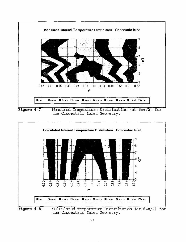
Measured Internal Temperature Distribution - Concentric Inlet

HB-8

Hi ^

. • : • , ; ; .

.... _.,.

HB-8

Hi ^ HB-8

Hi ^ • p E r | ^ ^ L HB-8

Hi ^ j r [^flBSB V -5

pnH|L_ ^^» i|BB si -5

-0.87 -0.71 -0.55 -0.39 -0.24 -0.08 0.08 0.24 0.39 0.55 0.71 0.87

r*

• 0-0.1 H 0.1-0.2 • 0.2-0.3 • 0.3-0.* •0.4-0.5 Q 0.5-0.6 • 0.6-0.7 S 0.7-0.8 • 0.8-0.9 • 0.3-1

Figure 4-7 Measured Temperature Distribution (at 6=rc/2) for the Concentric Inlet Geometry.

Calculated Internal Temperature Distribution - Concentric Inlet

10-0.1 H 0.1-0.2 • 0.2-0.3 • 0.3-0.* • 0.4-0.5 0! 0.5-0.6 • 0.6-0.7 • 0.7-0.8 • 0.8-0.3 • 0.3-1

Figure 4-8 Calculated Temperature Distribution (at 8=n/2) for the Concentric Inlet Geometry.

57

4.2.3 Effective Thermal Diffusivity Due To Turbulence

In Appendix D, the equations for turbulent fluid flow were presented using the Reynold's decomposition (equations D-12, D-13, and D-14). The treatment of the fluctuation cross-product terms led to the definition of the eddy viscosity model and the mixing length model (equations D-24 and D-25). These models give the following relations for the eddy viscosity and the eddy

diffusivity

--•"(f)

--•"(f)

The ratio of these two factors is a function of the Reynold's number, and can vary from 1 to 1.6. As an approximation, we will take them to be equal. To evaluate the eddy diffusivity, we use Prandtl's power law to represent the velocity profile

°(W u(r) = UU 7 4 " 1 4

where y is the distance from the pipe wall, U is the maximum velocity, and R is the pipe inner radius. The mixing length 1 will be expressed by the empirical relation (Nikuradse)

liy) = 0.14 - o.os/i - ^ ) 2 - o.oe/i - -^\4| 4-15

The resulting function for the eddy diffusivity is plotted in Figure 4-9.

58

Figure 4-9 Eddy Diffusivity For Turbulent Pipe Flow.

Integrating this function over the radius gives an average value for the eddy diffusivity of 5.4 x 1CT4 triys. The value of the molecular thermal diffusivity for saturated water at 37 °C is 1.5 x 10"7 mVs. The total thermal diffusivity is therefore just equal to 5.4 x 10"4 mVs. This is the value that is used in the results plotted in Figures 4-6 and 4-8.

4.3 Heat Transfer Through the Pipe Wall

The heat transfer from the fluid to the pipe wall is a function of the fluid velocity (Reynold's number) and the fluid conductivity (Prandtl number). The heat transfer coefficient can be calculated using empirical correlations such as the Dittus-Boelter correlation

NuD = Q.Q23Re%-3 Prn 4-16

59

where n = 0.3 for cooling and 0.4 for heating. The Nuselt number is defined as

NUD = M 4-17 Kf

where kf is the conductivity of the fluid. When the TSTF is operating at a mean flow velocity of 5 m/s, the Reynold's number is 5.4 x 105 and the Prandtl number is 4.62 (fluid properties evaluated at 37 °C). Thus the average value for the heat transfer coefficient is 1.36 x 104 W/m2K. The thermal resistance for this heat transfer coefficient at the pipe wall (radius R) is

Rconv 2nRhL 4 " 1 8

This is evaluated to 3.08 x 10"4 per meter of pipe axial length (L). The temperature difference between the fluid and the pipe wall is expressed as

A r = g r J ? c o n v 4 -19

where qr is the radial rate of heat flow. The heat flow rate at the wall of the pipe is on the order of 5 W, making the AT approximately 0.001 °C.

The thermal effect of the stainless steel pipe is evaluated in a similar manner. Thermal resistance through the wall is given by

J?_w = - ^ ^ l n l ^ l 4-20 cond 2

60

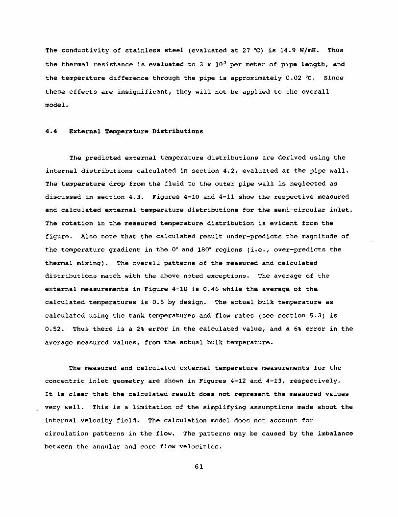
The conductivity of stainless steel (evaluated at 27 °C) is 14.9 W/mK. Thus the thermal resistance is evaluated to 3 x 10'3 per meter of pipe length, and the temperature difference through the pipe is approximately 0-02 °C. Since these effects are insignificant, they will not be applied to the overall model.

4.4 External Temperature Distributions

The predicted external temperature distributions are derived using the internal distributions calculated in section 4.2, evaluated at the pipe wall. The temperature drop from the fluid to the outer pipe wall is neglected as discussed in section 4.3. Figures 4-10 and 4-11 show the respective measured and calculated external temperature distributions for the semi-circular inlet. The rotation in the measured temperature distribution is evident from the figure. Also note that the calculated result under-predicts the magnitude of the temperature gradient in the 0° and 180° regions (i.e., over-predicts the thermal mixing). The overall patterns of the measured and calculated distributions match with the above noted exceptions. The average of the external measurements in Figure 4-10 is 0.46 while the average of the calculated temperatures is 0.5 by design. The actual bulk temperature as calculated using the tank temperatures and flow rates (see section 5.3) is 0.52. Thus there is a 2% error in the calculated value, and a 6% error in the average measured values, from the actual bulk temperature.

The measured and calculated external temperature measurements for the concentric inlet geometry are shown in Figures 4-12 and 4-13, respectively. It is clear that the calculated result does not represent the measured values very well. This is a limitation of the simplifying assumptions made about the internal velocity field. The calculation model does not account for circulation patterns in the flow. The patterns may be caused by the imbalance between the annular and core flow velocities.

61

Measured External Temperature Distibution, Semi-Circular Inlet, HC Stations.

135 180 225 Angular Position (degrees)

10-0.1 H 0.1-0.2 • 0.2-0.3 • 0.3-01 • 0>0.5 H 0.5-0.6 • 0.6-07 • 0.7-0.8 • 0.8-0.9 • 0.9-1

Figure 4-10 Measured External Temperature Distribution, Semi-Circular Inlet, HC Stations.

Calculated External Temperature Oistibution, Semi-Circular Inlet, HC Stations.

135 180 225 Angular Position (degrees)

270

10-0.1 • 0.1-0.2 • 0.2-0.3 • 0.3-0.4 • 0.1-0.5 • 0.5-0.6 • 0.6:0.7 • 0 7-0.8 • 0 8-0 9 0 0.9-1

Figure 4-11 Calculated External Temperature Distribution, Semi-Circular Inlet.

62

Measured External Temperature Oistibution, Concentric Inlet, HC Stations.

90 135 180 225 Angular Position (degrees)

270 315 360

10-01 H 0.1-0.2 •0.2-0.3 • 0.3-0.4 • 0.4-0.5 H 0.5-0.6 • 0,6-0.7 • 0.7-0.8

Figure 4-12 Measured External Temperature Distribution, Concentric Inlet, HC Stations.

1 Dak :ulal ted 1 Exte rna I T e Inle

mpe t, Hi

ratu C S l

ire 1 alio

l is t ns.

ibuti on, Cor icen trie

r9

• 6 °

•5

0 45 90 135 180 225 270 315 360 Angular Position (degrees)

• 0-0.1 B 0.1-0.2 fl 0.2-0.3 • 0.3-0.4 • 0.4-0.5 Q 0.5-0.6 fl 0.6-0.7 IB 0.7-0.8

Figure 4-13 Calculated External Temperature Distribution, Concentric Inlet, HC Stations.

63

5. EMPIRICAL METHODS FOR PREDICTING BULK TEMPERATURES

5.1 Introduction

The problem of measuring a flow that is not thermally well-mixed can be addressed by providing a finer mesh of measurement points to map the temperature field and perform a spatial averaging. A number of measurements need to be taken to develop a set of statistics adequate for an accurate bulk temperature estimate. This approach allows the determination of temperature distributions along the pipe perimeter under steady state flow conditions. Using only pipe surface measurements creates the possibility of temperature

masking. That is, if a thermally striped layer develops away from the pipe wall, and mixing is not sufficiently energetic in the radial direction, then the temperature of that layer of fluid will be masked from the surface measurements by the intervening fluid. The contribution to the bulk temperature estimate from the masked fluid will be diminished or lost. This experiment will also demonstrate this condition by producing conditions that will create this effect.

In this chapter, we will analyze the temperature data using two methods. First, a simple statistical approach will be used. The averages of groups of thermocouples will be taken to estimate the bulk temperature at each measurement station. Then the axial measurements will be used in conjunction with the group averages to try to predict trends that are developing within the fluid. The second technique will examine the application of artificial neural networks as a way to predict bulk fluid temperature from external measurements. A neural network model can be developed to weight the external measurements based on appropriate training patterns (i.e., temperature distributions).

64

5.2 Statistical Method

In this method, simple averages are calculated for different groupings of external thermocouples. The groups are listed in Table 5-1. For comparison to the group averages, the bulk temperature is calculated using the tank discharge temperature and volumetric flow rate for each individual tank. Note that the data at L/D=4 is interpolated.

Semi-Circular Inlet Geometry

Measurement results for the semi-circular inlet geometry are plotted in Figures 5-1 (HC stations) and 5-2 (CH stations). The bulk temperature measurement coincides with all of the group averages at an L/D=3. At this point, the two temperature regions have just begun to mix, and most thermocouples are, in equal proportion, measuring either T^ or T^. Thus the

Table 5-1 External Thermocouple Groups

Group No. Number of Sensors Angular Positions Idea)

1 4 0, 90, 180, 270 2 4 23, 113, 203, 293 3 4 45, 135, 225, 315 4 4 68, 158, 248, 338 5 8 0, 45, 90, 135

180, 225, 270, 315 23,68, 113, 158, 203, 248, 293, 338

16 All

65

Group Averages for External Thermocouples

0.550 T

S 0.500 IB t . 0)

I 0.450 I -"S 0.400 "5 E o 0.350 -Z

0.300 5 6 7

Axial Position (L/D) 10

- * — Bulk Temp

- • — Group 1

- * — Group 2

- ° — Group 3

- • Group 4

-*— Group 5

- • — Group 6

" • — Group 7

Figure 5-1 Group Averages for Semi-Circular I n l e t , HC S ta t ions .


0.700 T

£ 0.650

g. 0.600 £ £ 0.550 •a o | 0.500 £ J 0.450

0.400 4 5 6 7

Axial Position (L/D)

" • — Bulk Temp

- • — Group 1

- • — Group 2

-°— Group 3

- * — Group 4

- • — Group 5

" • — Group 6

" • — Group 7

Figure 5-2 Group Averages for Semi-Circular Inlet, CH Stations. 66

averages are very close to the bulk temperature. The averages then diverge from the bulk temperature (except at L/D=6). This divergence appears to level off around L/D=8, and begin to converge back to the bulk temperature at L/D=9. However, this convergence is not conclusive within the axial data range of the TSTF experiment.

The behavior between the HC stations and the CH stations mirror each other. In the HC case, the cold fluid is in the top half of the pipe, and dominates the external measurements as mixing progresses. For the CH case, the hot fluid is in the top half of the pipe, and the opposite trend is observed. There is clearly a hydrodynamic effect that allows the fluid in the top half of the pipe (from tank B) to circulate around the outer region of the pipe, thus biasing the external temperature measurements. As noted in Table 3-2, the flow rate from tank B is 4% higher than that from tank A. The velocity difference between the two streams results in a shear stress at the hot/cold interface, thus introducing an instability in the velocity field. This is the most likely cause of the flow pattern observed in the test results. Referring to Figure 3-2, the rotation in the temperature field (as measured by the external thermocouples) provides further evidence of this pattern. For this particular inlet condition, the group averages diverge as the fluid in the lower half of the pipe is masked by the circulation of the upper fluid around the inner wall of the pipe. As mixing progress, it is predicted that the average temperatures will converge on the bulk temperature. As noted above, this convergence is not conclusive within this data set. Temperature measurements taken at axial positions further downstream are necessary to confirm this.

Another important feature of the group averages is the group size. The groups that contain four measurements each are spread out. However, the groups of eight and sixteen thermocouples are nearly equal. Thus it appears that a good representation in the angular direction is two thermocouples per

67

quadrant. Fewer thermocouples increases the spread in the estimate, while more provides no additional accuracy. It is not as clear how many measurement stations are needed in the axial direction. For this inlet geometry, the first axial station give the best estimate, while the remaining stations become less accurate. Thus it would appear that if it is at the correct location, one is sufficient. However, an array of axial positions show the development of the temperature distribution, and can help to determine at what point the fluid temperatures become steady. That is, at what point dT/dx approaches zero.

Concentric Inlet Geometry

Measurement results for the concentric inlet geometry are plotted in Figures 5-3 (HC stations) and 5-4 (CH stations). The initial condition for this inlet geometry (HC case) is an annulus of fluid at temperature T c

surrounding a core of fluid at temperature T H (vice-versa for the CH stations). Thus the core fluid is initially masked by the annular fluid, and the group average is extremely biased toward T c. It is clear from the data that the pipe wall temperature is converging on the bulk fluid temperature. The asymptotic behavior of the group averages reflects the thermal diffusion of the core fluid through the annular fluid to the pipe wall. The axial distribution of a group average can be extrapolated to its asymptotic limit (i.e., the bulk temperature). For example, an s-curve of the form

, „ W+-> 5-1 gkt) = e x

can be fit to the group average data to estimate the asymptotic limit. Figures 5.5 and 5.6 show a possible fit of equation 5-1 to the group averages for the HC and CH stations respectively. The function parameters A and B were

68

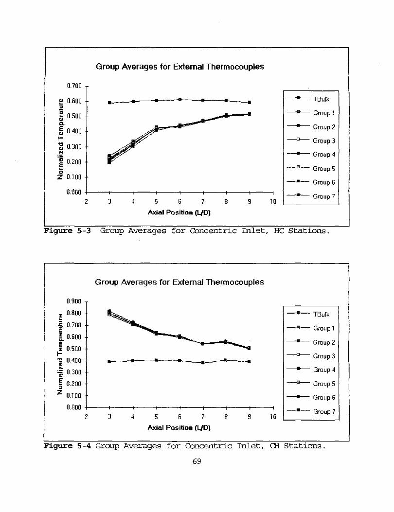
0.700

8 0.600

I 0.500 + a. I 0.400 4-

"O 0) 0.300

| 0.200 •-

Z 0.100 -•

0.000


5 6 7

Axial Position (LJD) 10

_s_

TBulk

Group 1

Group 2

Group 3

Group 4

Group 5

Group 6

Group 7

Figure 5-3 Group Averages for Concentric Inlet, HC Stations.

0.900

u 0.800 4-

I 0.700

| 0.600

a) 0.500 -•

•o 0.400 4-

= 0.300 4-

| 0.200 4-Z 0.100 4-

0.000


5 6 7 Axial Position (\JD)

10

Figure 5-4 Group Averages for Concentric Inlet, CH Stations, 69

0.6

0.4

0.2

*

____Z-L^ * " "

- f | , i -1 ,

' / i

t f t 1 I I

! j i | 1 !

< i

, 1 1

J : j \

* i

.« f

1 i

i i ! 1

0.5 1 1J Ami Eistaioa (m)

2.5

Figure 5-5 Extrapolation of Group Averages for the Concentric Inlet Geometry, HC Stations.

i

u "8 u 4'' s. 0.8 6

1 0.6 o

0.4

i

u "8 u 4'' s. 0.8 6

1 0.6 o

0.4

i j i «

i i

\ |

! i i j r 1

J j j

i

u "8 u 4'' s. 0.8 6

1 0.6 o

0.4

i j i «

i i

\ | i 1 i \ \ * 1 i !

,

i

u "8 u 4'' s. 0.8 6

1 0.6 o

0.4

• *v

j

~ r ! T ~ — : i j { -- i I j j

,

i

u "8 u 4'' s. 0.8 6

1 0.6 o

0.4 0 0.5 1 1.5 2

Axial Distance (mj 2.5 3

Figure 5-6 Extrapolation of Group Averages for the Concentric Inlet Geometry, CH Stations.

70

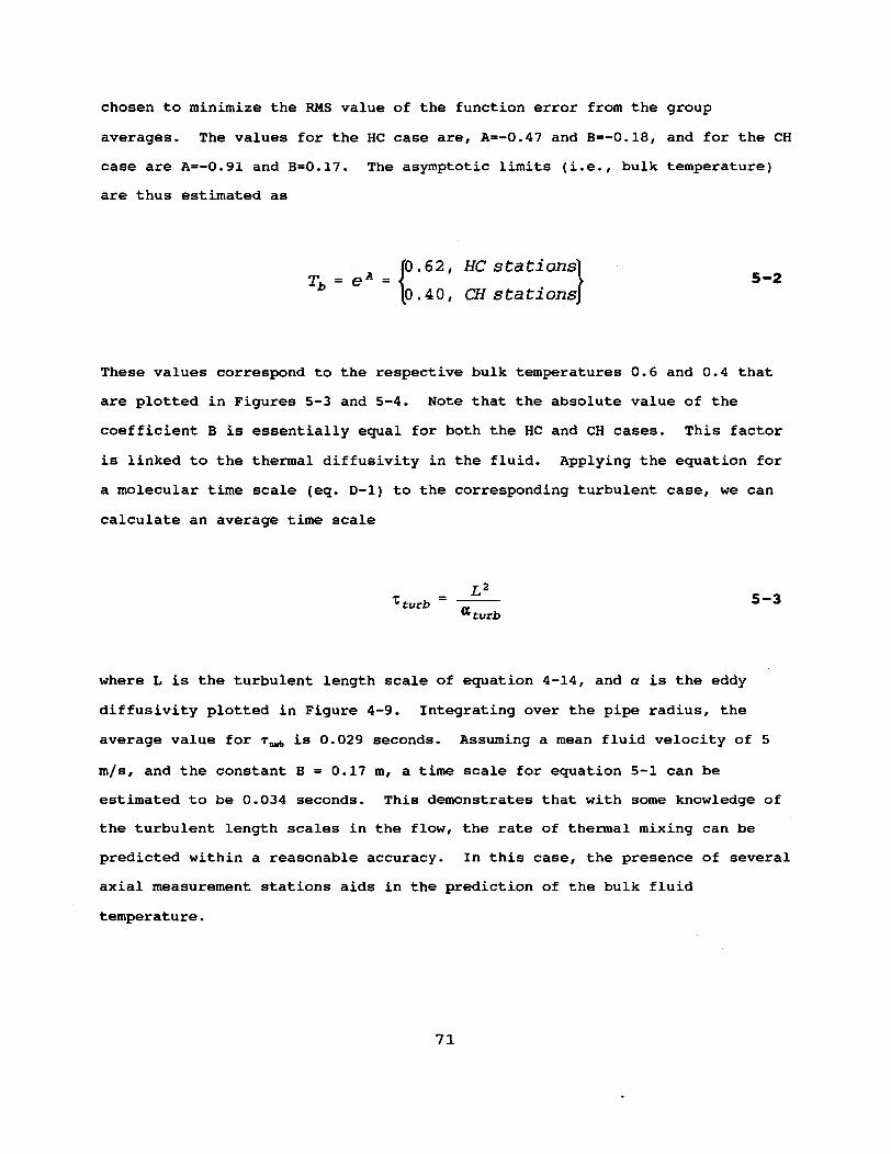
chosen to minimize the RMS value of the function error from the group averages. The values for the HC case are, A=-0.47 and B=-0.18, and for the CH case are A=-0.91 and B=0.17. The asymptotic limits (i.e., bulk temperature) are thus estimated as

_ JO. 6 2 , " jo -40 ,

HC stations) \ 5 " 2

* ' " CH stations]

These values correspond to the respective bulk temperatures 0.6 and 0.4 that are plotted in Figures 5-3 and 5-4. Note that the absolute value of the coefficient B is essentially equal for both the HC and CH cases. This factor is linked to the thermal diffusivity in the fluid. Applying the equation for a molecular time scale (eq. D-1) to the corresponding turbulent case, we can calculate an average time scale

xturb — 5 ~ 3

aturb

where L is the turbulent length scale of equation 4-14, and a is the eddy diffusivity plotted in Figure 4-9. Integrating over the pipe radius, the average value for T ^ is 0.029 seconds. Assuming a mean fluid velocity of 5 m/s, and the constant B = 0.17 m, a time scale for equation 5-1 can be estimated to be 0.034 seconds. This demonstrates that with some knowledge of the turbulent length scales in the flow, the rate of thermal mixing can be predicted within a reasonable accuracy. In this case, the presence of several axial measurement stations aids in the prediction of the bulk fluid temperature.

71

5.3 Artificial Neural Networks

A bulk temperature estimate may be obtained by studying the empirical relationship between the pipe surface temperature and bulk fluid temperature measured under different internal temperature distributions. The method applied in this section uses the associative ability of the neural network paradigm. One of the most commonly used learning algorithms, namely Backpropagtion Neural Network (BPN), is utilized to develop a relationship between the measured external temperatures and fluid bulk temperature.

The analysis uses artificial neural networks technology to develop a relationship between bulk fluid temperature measurements and pipe surface temperature measurements. One of the design goals of the TSTF was to produce consistent, repeatable flow conditions (i.e., bulk temperature). As a consequence, while the results of the neural network analysis are promising, they are restricted by the dynamic range of the measured data which covers a very limited range of bulk temperature values. Therefore, the results are not conclusive, but illustrate the potential feasibility of applying artificial neural network modeling for estimating bulk fluid temperature.

Training the Neural Network Model

The neural network is designed to accept the surface temperatures as inputs, and the bulk fluid temperatures as the desired outputs. The error between the predicted bulk fluid temperatures and the desired bulk temperatures is used by the learning algorithm to increase the accuracy of the network model. Training the network is an iterative process that is repeated until the prediction error becomes acceptable.

Pre-Processing the Data

One of the important steps in developing neural network models is the preparation of the training data. There are various ways of normalizing the

72

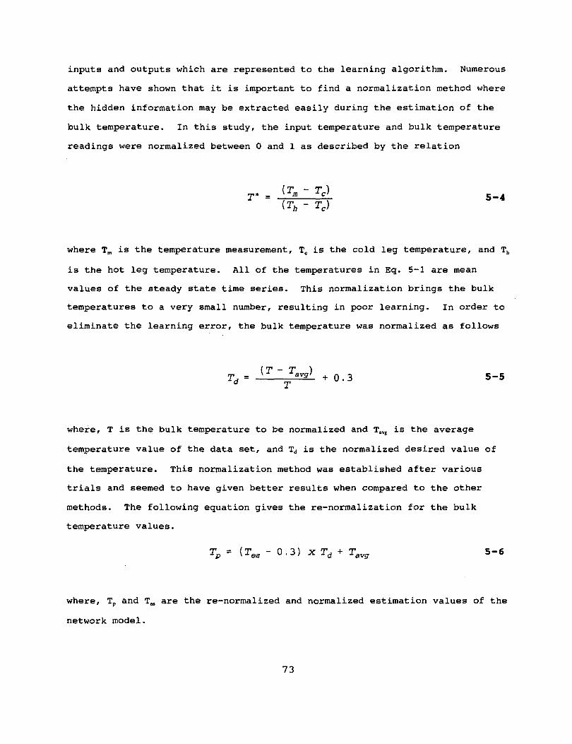
inputs and outputs which are represented to the learning algorithm. Numerous attempts have shown that it is important to find a normalization method where the hidden information may be extracted easily during the estimation of the bulk temperature. In this study, the input temperature and bulk temperature readings were normalized between 0 and 1 as described by the relation

(T - T ) T* = ±1* l£i 5-4

(Tb ~ Tc)

where T m is the temperature measurement, Tc is the cold leg temperature, and Th

is the hot leg temperature. All of the temperatures in Eq. 5-1 are mean values of the steady state time series. This normalization brings the bulk temperatures to a very small number, resulting in poor learning. In order to eliminate the learning error, the bulk temperature was normalized as follows

(T - T ) 11 a yg ; +0.3 5-5

where, T is the bulk temperature to be normalized and Tavg is the average temperature value of the data set, and Td is the normalized desired value of the temperature. This normalization method was established after various trials and seemed to have given better results when compared to the other methods. The following equation gives the re-normalization for the bulk temperature values.

Tn = (Tes - 0.3) X Trf + Tava 5-6

where, Tp and T M are the re-normalized and normalized estimation values of the network model.

73

Estimation Results

The network t r a i n i n g used twelve d i f f e r e n t da ta s e t s , and e s t i m a t i o n s of

t h e network model were encouraging. The l a r g e s t e s t i m a t i o n e r r o r was l e s s

than 0.01°C. Following t a b l e shows the d e s i r e d ( a c t u a l ) and t h e e s t ima ted

va lues of bulk t empera ture obta ined from one of t h e developed n e u r a l network

models.

Table 5-2 - D e s i r e d v s . P r e d i c t e d Bulk T e m p e r a t u r e s from N e u r a l Network Model

Bulk Temperature Model Es t imate 4 0 . 3 5 2 4 0 . 3 5 0 3 9 . 8 0 9 39 .814 4 0 . 1 3 0 40 .126 4 1 . 7 6 2 41 .762 4 1 . 8 7 0 41 .874 4 3 . 2 0 0 4 3 . 1 9 8 4 1 . 5 9 1 4 1 . 5 8 9 4 1 . 3 2 4 41 .326 4 0 . 7 4 4 40 .744 4 0 . 7 0 1 40 .700 4 0 . 3 8 8 4 0 . 3 8 9 4 0 . 0 0 0 4 0 . 0 0 0

74

6. CONCLUSIONS

This study shows that it is possible to estimate the bulk temperature of a fluid from measurements of the surface temperature of the pipe. However, some inlet conditions made accurate determination of the bulk temperature difficult by masking temperature stripes in the flow from the pipe wall. A more complex model could be developed that carefully examines data from multiple axial locations to better estimate bulk temperature for these circumstances. This strategy would certainly work for the controlled circumstances of the experiment.

The time response of the system is limited by the conduction path through the pipe wall to the external thermocouples. The time response of the experimental system was of the order of 10 seconds. This is demonstrated by the time trace of the external thermocouples given in Figure C-2. The response is due to the transient conduction in the pipe that follows a change in the adjacent fluid temperature. This transient conduction problem is considered in Appendix F for an idealized change in the fluid temperature from uniform at 36.5 Degrees Celsius to 45 Degrees Celsius in the top half of the pipe and 18 Degrees Celsius in the bottom half of the pipe. The pipe was modeled in the ABAQUS code and the results given in Figures Fl through F3 show the transient response occurs in around 10 seconds. Note that the steady state solution to the striped flow boundary condition given in Figure F4 indicates that the azimuthal conduction effects extend over roughly three pipe thicknesses. Therefore, placing thermocouples closer than three pipe thicknesses around the pipe circumference will not significantly improve the knowledge of the spatial distribution in the external pipe temperature.

The measured temperature distributions inside the pipe downstream of the inlet show well the effects of turbulent mixing and turbulent diffusivity.

75

The simple models for turbulent diffusivity employed in this study predicted the measured relaxation in the temperature profile in the pipe as the flow moved downstream. Knowledge of the thermal diffusivity in conjunction with some knowledge of the inlet conditions allows the thermal gradients to be bounded as a function of axial location downstream. This allows the possible error in the predicted bulk temperature value to be bounded when the prediction technique utilizing the mean temperature value is employed.

76

APPENDIX A - DUKE POWER MEETING ATTENDEES

Name Melvin Cline Dale Smith Jeff Nolin J. Michael Davis Dan Wellbaum Mike Mallard Arthur Ruggles

Organization Duke Power Duke Power Duke Power Duke Power Duke Power Duke Power University of Tennessee

A-l

APPENDIX B - SENSOR CALIBRATION

The calibration of the thermocouples is checked using the two reference thermocouples that are installed in the discharge pipes for tank A and tank B. A hot oil bath was used to verify the calibration of the reference thermocouples. The reference thermocouples are re-installed into the TSTF, and are then used to perform an in-situ check of the calibration of the test spool thermocouples. They are also used to measure the temperature of the supply tank water at the discharge of each tank.

During the calibration of the TSTF instrumentation, it was noted that the data acquisition system introduced a bias in the sensor measurements. The bias is a result of the cold junction temperature varying across the thermocouple termination board. Cold junction compensation is provided at one point within the data acquisition enclosure. Since each thermocouple is not individually compensated, internal temperature variances inside the data acquisition enclosure can introduce a bias error. We attempted to reduce this effect by placing the data acquisition enclosure within a ventilated box, thus drawing air across the termination board, and reducing the temperature gradient. Even using the ventilated box, the system still introduced a bias in the measurements. To help quantify this bias, we use a group bias and reference bias for each thermocouple.

The group bias is a measure of the average deviation (i.e., accuracy) of an individual thermocouple from the group of redundant sensors. The internal and external thermocouples each form one group. For a given set of measurements taken under isothermal conditions, the average for each thermocouple is calculated, and then a group average is determined. The deviation of each thermocouple from it's group average is called the group

B-l

bias for that thermocouple. The reference bias is a measure of the average deviation of an individual thermocouple from the reference thermocouple measurement. This parameter can be used to correct thermocouple measurements (if desired) to the reference thermocouple measurements.

The results of the calibration check are presented in Table 2-3. For each thermocouple, the standard deviation, 95% confidence interval (i.e., 3o interval), the absolute value of the group bias, and reference bias are presented. The average value of the 95% confidence interval for is 0.12 °C for group A, and 0.14 °C for group B. The average group deviation is 0.10 °C for group A and 0.17 °C for group B. Thus the accuracy of the thermocouples within their respective groups is on the order of <0.2 °C, or 0.4% of full scale (i.e., 50 °C). However, the reference bias (cold junction bias effect) increases the absolute error significantly. Note that the average reference bias for group A and group B is -1.25 °C and -1.36 °C respectively. This error yields an overall error of <3% of full scale. Thus the reference bias is applied to each individual sensor channel to help compensate for the cold junction bias.

B-2

Table B-1 Thermocouple Calibration Data.

TIC Nwmher.-.. Standard-Deviation— rV.nfiHpnP* fQSU\ Gfmin Bias —Reference Bias—

Ref. A 0.053 0.16 n/a n/a

Ref. B 0.071 0.21 n/a n/a

Al 0.043 0.13 0.09 -1.34

A2 0.046 0.14 0.11 -1.37

A3 0.045 0.13 0.10 -1.35

A4 0.044 0.13 0.08 -1.33

A5 0.040 0.12 0.07 -1.33

A6 0.039 0.12 0.06 -1.31

A7 0.074 0.22 0.07 -1.33

A8 0.042 0.12 0.05 -1.30

A9 0.034 0.10 0.06 -1.19

A10 0.029 0.09 0.09 -1.16

A l l 0.033 0.10 0.13 -1.13

A12 0.034 0.10 0.17 -1.09

A13 0.034 0.10 0.18 -1.07

Bl 0.048 0.14 0.34 -1.70

B2 0.047 0.14 0.21 -1.58

B3 0.045 0.13 0.25 -1.62

B4 0.052 0.16 <0.01 -1.37

B5 0.043 0.13 0.12 -1.24

B6 0.043 0.13 0.07 -1.43

B7 0.044 0.13 0.18 -1.18

B8 0.045 0.14 0.11 -1.25

B9 0.049 0.15 0.03 -1.39

BIO 0.052 0.16 0.15 -1.51

Bl l 0.049 0.15 0.19 -1.55

B12 0.050 0.15 0.40 -0.96

B13 0.052 0.16 0.05 -1.31

B14 0.045 0.13 0.13 -1.50

B15 0.051 0.15 0.12 -1.25

B16 0.047 0.14 0.38 -0.98

B-3

APPENDIX C - SAMPLE OF RAW DATA POST PROCESSING

This appendix describes the methodology used to process the raw temperature data acquired in the Thermal Stratification Test Facility (TSTF). Sensor data is sampled once per second and output to a text file for later analysis. The test spool piece is instrumented with 16 external thermocouples and 12 internal thermocouples (see section 2.2). There are also two thermocouples located on the discharge pipe of each supply tank. Finally, each supply tank has a pressure transducer to help measure the supply flow rates. Thus, there are a total of 32 time series associated with a measurement run (30 thermocouple signals and 2 pressure transmitter voltage signals). These time series comprise the raw data for a given measurement run.

A typical example (Figure C-l) shows the time series for a measurement run at station HC1-I for the internal measurements. The time series of the external sensors for the same measurement run is shown in Figure C-2. To complete the set, Figure C-3 shows the supply tank temperature outputs and Figure C-4 shows the supply tank levels. A typical measurement run will last for approximately 60 seconds at a flow velocity of 5 m/s.

The desired information from the raw data is the steady state temperature measurements for each sensor. Figure C-l shows the behavior of the internal measurements. The two sensors located near the center of the pipe demonstrate the effect of fluid turbulence along the hot/cold interface. Moving away from the pipe centerline, the variance of the temperature fluctuations drops off significantly (at least, for this measurement station). Thus the accuracy of the mean values of these temperature measurements (as an estimate of the fluid temperature) increases away from the pipe centerline.

C-l

Time Series of the Internal Thermocouples - Station HCl-l

120

A1

A2

A3

A4

. A5

A6

A8

A9

A10

All

A12

A13

Figure C-l - Time Series of Internal Temperature Measurements.

tem

pera

ture

(C

)

55

50

45

40

35

30

25

20

C

tem

pera

ture

(C

)

55

50

45

40

35

30

25

20

C

Time Series of External Temperatures - Station HC1-I

-—•—

-—-»—

-—a—

m—

•—

„ B 1

82

_ 83

_ B 4

B5

86

B7

_ B 8

B9

__B10

811

812

_ 8 1 3

_ 8 1 4

_ 815

p i f l

tem

pera

ture

(C

)

55

50

45

40

35

30

25

20

C

~ r """""" ' i "" I |

-—•—

-—-»—

-—a—

m—

•—

„ B 1

82

_ 83

_ B 4

B5

86

B7

_ B 8

B9

__B10

811

812

_ 8 1 3

_ 8 1 4

_ 815

p i f l

tem

pera

ture

(C

)

55

50

45

40

35

30

25

20

C

T&fe>^ I

-—•—

-—-»—

-—a—

m—

•—

„ B 1

82

_ 83

_ B 4

B5

86

B7

_ B 8

B9

__B10

811

812

_ 8 1 3

_ 8 1 4

_ 815

p i f l

tem

pera

ture

(C

)

55

50

45

40

35

30

25

20

C

LmtttiH'ff'ft-uiijJ T&fe>^ I

-—•—

-—-»—

-—a—

m—

•—

„ B 1

82

_ 83

_ B 4

B5

86

B7

_ B 8

B9

__B10

811

812

_ 8 1 3

_ 8 1 4

_ 815

p i f l

tem

pera

ture

(C

)

55

50

45

40

35

30

25

20

C

-—•—

-—-»—

-—a—

m—

•—

„ B 1

82

_ 83

_ B 4

B5

86

B7

_ B 8

B9

__B10

811

812

_ 8 1 3

_ 8 1 4

_ 815

p i f l

tem

pera

ture

(C

)

55

50

45

40

35

30

25

20

C

-—•—

-—-»—

-—a—

m—

•—

„ B 1

82

_ 83

_ B 4

B5

86

B7

_ B 8

B9

__B10

811

812

_ 8 1 3

_ 8 1 4

_ 815

p i f l

tem

pera

ture

(C

)

55

50

45

40

35

30

25

20

C

-—•—

-—-»—

-—a—

m—

•—

„ B 1

82

_ 83

_ B 4

B5

86

B7

_ B 8

B9

__B10

811

812

_ 8 1 3

_ 8 1 4

_ 815

p i f l

tem

pera

ture

(C

)

55

50

45

40

35

30

25

20

C

m ^ N l ^ ^ ^ ^ J

-—•—

-—-»—

-—a—

m—

•—

„ B 1

82

_ 83

_ B 4

B5

86

B7

_ B 8

B9

__B10

811

812

_ 8 1 3

_ 8 1 4

_ 815

p i f l

tem

pera

ture

(C

)

55

50

45

40

35

30

25

20

C

-—•—

-—-»—

-—a—

m—

•—

„ B 1

82

_ 83

_ B 4

B5

86

B7

_ B 8

B9

__B10

811

812

_ 8 1 3

_ 8 1 4

_ 815

p i f l

tem

pera

ture

(C

)

55

50

45

40

35

30

25

20

C

a—

„ B 1

82

_ 83

_ B 4

B5

86

B7

_ B 8

B9

__B10

811

812

_ 8 1 3

_ 8 1 4

_ 815

p i f l

tem

pera

ture

(C

)

55

50

45

40

35

30

25

20

C I .__

»o

„ B 1

82

_ 83

_ B 4

B5

86

B7

_ B 8

B9

__B10

811

812

_ 8 1 3

_ 8 1 4

_ 815

p i f l

tem

pera

ture

(C

)

55

50

45

40

35

30

25

20

C ) 20 40 60 80 100 12

time |s)

»o

„ B 1

82

_ 83

_ B 4

B5

86

B7

_ B 8

B9

__B10

811

812

_ 8 1 3

_ 8 1 4

_ 815

p i f l

tem

pera

ture

(C

)

55

50

45

40

35

30

25

20

C

Figure C-2 - Time Series of External Temperature Measurements. C-2

60

Supply Tank Discharge Temperature - Run HC1071

20 40 60 X

50 B

4 0 r m • —

30

1

_ A _ _ — _ _ • X

20

10 —•— Tank A Temp |

_ T a nk B Temp ! _ T a

0 ~ T

80 100 120

Figure C-3 - Time Series of Supply Tank Discharge Temperature.

0.79

0.78

0.77

0.76

m 0.75 to % 0.74 >

0.73

0.72

0.71

0.7 C

i ^ B B M a ^ .

Time Series of the Supply Tank Level - Run HC1071

0.79

0.78

0.77

0.76

m 0.75 to % 0.74 >

0.73

0.72

0.71

0.7 C

i ^ B B M a ^ . ! 0.79

0.78

0.77

0.76

m 0.75 to % 0.74 >

0.73

0.72

0.71

0.7 C

T^^^d^a- «— Tank A Lvl j

0.79

0.78

0.77

0.76

m 0.75 to % 0.74 >

0.73

0.72

0.71

0.7 C

^^^ , % , * * l * f a . m— Tank B Lvl i

0.79

0.78

0.77

0.76

m 0.75 to % 0.74 >

0.73

0.72

0.71

0.7 C

^ ^ ^ " ^ ^ i ^ _ !

0.79

0.78

0.77

0.76

m 0.75 to % 0.74 >

0.73

0.72

0.71

0.7 C

^ ^ ^ " ^ ^ i ^ _

0.79

0.78

0.77

0.76

m 0.75 to % 0.74 >

0.73

0.72

0.71

0.7 C

0.79

0.78

0.77

0.76

m 0.75 to % 0.74 >

0.73

0.72

0.71

0.7 C

0.79

0.78

0.77

0.76

m 0.75 to % 0.74 >

0.73

0.72

0.71

0.7 C

0.79

0.78

0.77

0.76

m 0.75 to % 0.74 >

0.73

0.72

0.71

0.7 C

0.79

0.78

0.77

0.76

m 0.75 to % 0.74 >

0.73

0.72

0.71

0.7 C

0.79

0.78

0.77

0.76

m 0.75 to % 0.74 >

0.73

0.72

0.71

0.7 C

0.79

0.78

0.77

0.76

m 0.75 to % 0.74 >

0.73

0.72

0.71

0.7 C

0.79

0.78

0.77

0.76

m 0.75 to % 0.74 >

0.73

0.72

0.71

0.7 C ) 20 40 60 80 100 1

time (s)

20

Figure C-4 - Time Series of Supply Tank Level, C-3

The external measurements do not exhibit the rapid fluctuations of the internal measurements. This is due to the increased thermal lag associated with the conductance through the stainless steel pipe. However, note that some of the external measurement have not yet achieved a true steady state (i.e., statistically stationary) condition. These measurements are associated with the hot/cold interface, in this case along the 0° and 180° locations. In this example, the length of the test run is not sufficiently long to reach a steady state condition. Thus the error of the mean values of these temperature measurements (as an estimate of the pipe surface temperature) will be greater than for a true steady state condition.

The calculation of the mean temperatures involves isolating a segment of the test run for which the temperatures most closely approach a steady state condition. In general, the endpoint of such a segment is at the end of the test run. This is best determined by using the pump shutoff time as determined in Figure C-4 (in this instance, pump shutoff is at 78 seconds). It is desirable to obtain as large a sample space as possible. However, as the size of the sample space grows, measurements taken in the transient phase of the test run will begin to bias the mean value. This is particularly true for the external measurements (Figure C-2).

To help select the optimal sample size, the standard deviations of the signals are calculated and plotted in Figures C-5 and C-6. The graphs show the standard deviations for different size sample groups (ranging from 10 elements to 50 elements). The standard deviations for the internal sensors show a sharp peak for sensors located near the centerline of the pipe. This reflects the turbulent nature of the temperature field in this area of the pipe. Notice that the standard deviations of the smallest sample group (10 elements) departs from the other sample groups in this region. This indicates that this sample group is too small. Figure C-6 shows the standard deviations for the external measurements. The magnitude of the temperature

C-4

Figure C-5 - Effect of Sample Size on Standard Deviation for Internal Measurements.

Effect of Sample Size on Temperature Standard Deviation - External

External Sensor No.

Figure C-6 - Effect of Sample Size on Standard Deviation for External Measurements.

C-5

fluctuations are much smaller for the external measurements due to the thermal lag associated with the pipe. There are two peaks that occur for all sample groups at sensors 2 and 9. This corresponds to the positions near sides of the pipe, where the temperature interface is located. However it is clear from the chart that the largest sample group (50) is biased around the entire pipe circumference. This sample group extends back into the part of the time series (Figure C-2) that is still in transient, and thus is too large. This leaves the sample groups 20, 30, and 40 as possible sample sizes. Thus most of the test runs will have an average sample size of 30 elements.

The next step in the methodology is to combine the mean temperatures for two or more test runs at a given station. This is done to confirm that a test run made at a station is repeatable. Figure C-7 shows the internal mean temperature values for two test runs made at station HC1-I. Figure C-8 shows the external temperatures for the same test runs. These two runs are averaged together to produce a representative temperature profile for station HC1-I. Temperature profiles for other stations are developed, and presented together graphically as shown in Chapter 3.

C-6

I o 2

1

0.9

0.8

0.7

0.6

0.5

0.4

0.3

0.2

0.1

0

-0.1

Semi-Circular Inlet - Internal Temperatures (HC1)

' 5 5 = *^=« ,

t.

x * = =

10 20 30 40 50 Distance from bottom of pipe (mm)

60

HC1069

HC1071

70 80

Figure C-7 - Mean Internal Temperatures - Station HC1-I.

Semi-Circular Inlet - External Temperatures (HC1)

90

67.5 113

\ 0.8

22.5

338

315 F

158

180

203

270

HC1069

HC1071

HC1069

HC1071

HC1069

HC1071

Figure C-8 - Mean External Temperatures - Station HC1-I C-7

APPENDIX D - BACKGROUND ON TURBULENCE AND MIXING THEORY

Turbulence originates when small disturbances in fluid streamlines are not damped out but instead enhanced. The likelihood of this occurring is evidenced by the Reynolds number (the ratio of inertia to viscous forces.) At high Reynolds number the disturbances are amplified by the inertial forces rather than dissipated by the viscous forces. Laminar pipe flow becomes turbulent at Reynold's numbers greater than 2,000. Other flows such as free shear flows may become unstable at much lower Reynold's numbers. Unfortunately the interaction between viscous terms and non-linear inertia terms in the equations of fluid motion are very complex. This combined with other features of turbulence such as randomness make it challenging to model mathematically.

As mentioned, turbulence is characterized by the existence of random fluctuations in the fluid. With a device such as a hot wire or laser anemometer these temperature and velocity fluctuations may be measured. Turbulence may also be characterized as being dissipative; significant viscous losses increase the internal energy of the fluid as they decrease the kinetic energy. Hence turbulence will decay unless energy is supplied to make up for these losses. Turbulent flows are generally shear flows and shear in the mean flow is a common source of this required energy.

Turbulence is advantageous as it provides an increase in heat and mass transfer rates. The rates of transfer and mixing are several orders of magnitude greater than their molecular counterparts. This leads to a flat temperature and velocity profile in fully developed pipe flows with steep gradients near the walls. Thus there are larger surface shear stresses (deleterious effect) but also larger heat and mass transfer rates ( desired

D-l

effect.) A simple scaling exercise can help to quantify these effects.

A scaling analysis of the equation for molecular diffusion with a fixed length scale results in

*«!• " ^ D - X

where L is a characteristic length scale and a is the thermal diffusivity. Now let L also represent the characteristic length scale of the turbulent motion and u represent a characteristic turbulent velocity fluctuation. Then dimensionally

I**, = i D - 2

The ratio of the turbulent time scale to the molecular time scale is

T turb _ a *mole u L

D-3

For fluids such as air and water the Prandtl number is close to unity and we can rewrite the above as

xtuzb _ _V_ _ _1_ D _ 4

However in most turbulent flows there is no one characteristic length scale and this exercise can only be used to indicate orders of'magnitude. In fact turbulence offers a range of length scales; from the dimension of the flow field down to the Kolmogrov microscale. Generally speaking large eddys (scaling with the width of the flow) are responsible for the transport of

D-2

momentum, particles, heat etc. Small scale eddys have an interesting relationship with the turbulent viscosity and turbulent energy dissipation which has been extensively analyzed by Kolmogrov.

The differential equations which govern the motion of a vector or scaler within a flowing fluid are derived by examining a stationary elemental control volume in the flow field. The conservation law is applied to the quantities of mass, momentum and energy to obtain a balance for each.

Mass

|H + |I = 0 D-5 dx dy

Momentum

Energy

dt dx dy p dx p\dx2 dy2,

dt dx dy ~ pCp\dx2 dy2)

D-6

D-7

Under certain conditions and with certain assumptions (such as those used in boundary layer analysis) mathematical solutions for the temperature and velocity profiles of laminar flow can be found. Turbulent flows contain energy fluctuations at frequencies from zero to 10kHz or more. A description of the flow at all points and times would be impossible. Reynolds suggested some of the difficulty associated with instantaneous turbulence could be eliminated if one considered the mean behavior averaged over a long enough period of time. It is the time mean behavior of turbulent flows that is of practical interest. With this in mind the equations for laminar flow may be converted into the time-averaged equations for turbulent flow by substitution

D-3

of certain parameters by their time averaged counterpart. These modified equations are called the Reynold's-averaged mean-motion equations.

The Reynold's decomposition is given by

Uy = Uy+ U' D _ 8

P = P + P' %• = x + T1

Before substituting these time averaged parameters into the equations it is useful to review algebra associated with time averaged and fluctuating components.

The quantities with an overbar represent mean values obtained by averaging over time, for example

to U = A fudt D-9

'0

Thus the quantities with a prime (fluctuating components) average to zero over time. The average is taken over a time that is large compared with the period of a typical fluctuation, and if T is independent of time, the time-mean flow is said to be steady.

to >dt = 0 D ~ 1 0 /„'<

These two d e f i n i t i o n s r e s u l t in t h e following

D-4

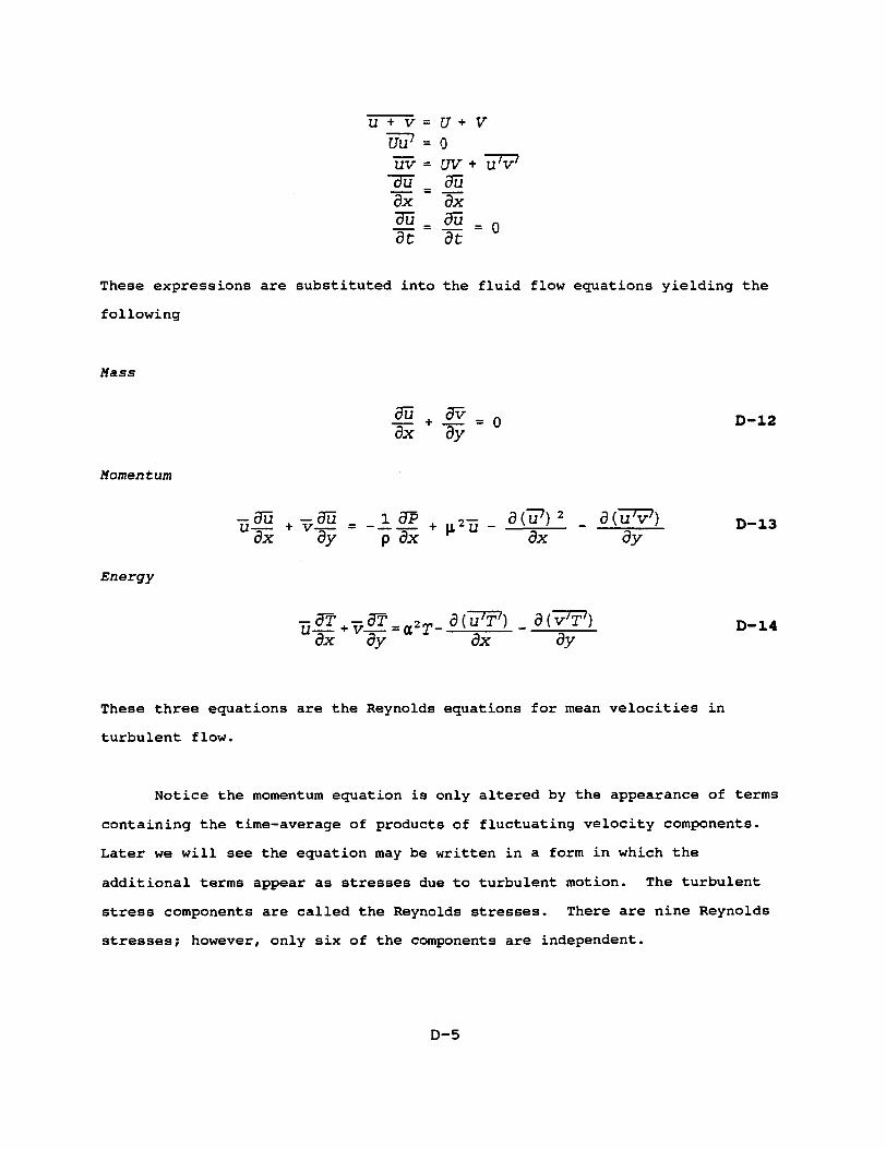
u + v = U + V ~uiP = 0

uv = uv + u V du _ £Ju ax dx d~u du ^ n

at at

These expressions are substituted into the fluid flow equations yielding the following

Mass

in + i r = 0 D-12 ax ay

Momentum

u J « + vJ?H - - i 5P + 2 - _ a o ? ) 2 _ djWV) D _ 1 3

ax ay p dx dx dy

Energy

u^+v^=a2T-l^Tl-ilrTl D - 1 4 dx dy dx dy

These three equations are the Reynolds equations for mean velocities in turbulent flow.

Notice the momentum equation is only altered by the appearance of terms containing the time-average of products of fluctuating velocity components. Later we will see the equation may be written in a form in which the additional terms appear as stresses due to turbulent motion. The turbulent stress components are called the Reynolds stresses. There are nine Reynolds stresses; however, only six of the components are independent.

D-5

Notice also that the energy equation is similar to the original but for the additional terms containing time-averages of products of fluctuating velocities and temperature. We will see that the energy equation may be rewritten to allow these extra terms to appear as heat fluxes which are due to the convective action of the turbulent motion. Also notice that the energy equation is similar in form to the momentum equation except temperature is a scaler compared to velocity.

We now have five equations and 14 unknowns. Thus there exist a closure problem. Also note that the turbulent stresses are controlled by differential equations and, unlike pure viscous stresses, are not simply related to the local rates of strain. The problem of these additional terms may be solved by representing them as dependent variables (e.g. the k-e model). Or it may be solved by specifying the correlations as functions of known quantities, for example by Prandtl's mixing length, or the turbulent Prandtl number approach.

A first step toward this goal is the use of assumptions found in boundary layer theory to simplify the equations.(i.e. normal stresses negligible compared to shear, etc)

^H>^r D-is dy dx

Boundary layer equations may be written as follows

uB + v|H = -1& + v- H - 4-W^) D-16 dx dy p ax dy2 dy

u|? + v-p = a f | - 4-TPF) D-17 dx dy dy2 dy

D-6

A simple conceptual model, which is widely used attributes the transport of momentum, heat, and mass in a turbulent boundary layer to the motion of eddies, small portions of fluid in the boundary layer that move about for a short time before losing their identity. Because of this motion, the transport of momentum, energy, and species is greatly enhanced. The notion of transport by eddies has prompted the introduction of a transport coefficient defined as the eddy diffusivity for momentum, heat and mass transfer. These are sometimes referred to as turbulent viscosity and turbulent diffusivity. With this in mind we can rewrite the equations to maintain the same form as the laminar version but the coefficients (viscosity, diffusivity, conductivity) are apparent ones composed of the laminar or molecular component plus a turbulent component which is often much greater (ten times) than the laminar value. A basic problem when dealing with turbulence is determining the value of these eddy diffusivities using the mean properties of the flow. Whereas molecular diffusivites are fluid properties, eddy diffusivities depend on the nature of the flow and vary from point to point in the flow.

It is useful to rewrite these as

u<® + v^- = -±& * ±J- (uJH - olFP) D-18 ox dy p dx p dy ay

u|I + vB = -±J?- {k£ - PC^F) D-19 ox dy pcp dy dy

There are three main types of turbulence models. The first two depend on the assumption made by Boussinesg (1877) that the stress-strain law for time-averaged turbulent flow could be represented in the same form as for laminar flow, i. e., as a product of the mean velocity gradient and a viscosity. Model type one finds the turbulent viscosity by way of an algebraic expression involving the mean velocity profile. Model type two uses differential equations to determine a turbulent viscosity. The third type

D-7

model does not attempt to provide effective turbulent transport quantities but actually uses differential transport equations for the turbulent fluxes. Some algebraic expressions for turbulent viscosity include Prandtl's mixing length hypothesis, von Karman's similarity hypothesis and the eddy viscosity formula. Differential models for turbulent viscosity include Prandtl's model (1945), Nee and Kovaszney's model (1968), and Kolmogrov's model (1942).

To correspond with our notion of shear stress and heat flux viewed as a molecular component enhanced by a turbulent component let us define a turbulent (eddy) shear stress and heat flux

Turbulent shear stress

du

Turbulent heat flux

- p W = pe„|H D-2 0

BT •pcplPF = pcPtH^ D-21

Substituting these new definitions into the boundary layer equations results in

u^ + v ^ = -!<* + 4- [ ( v + e M ) | H ] D-22 dx dy p dx dy M dy

u^ + v | ? = 9 [ (« + e „ ) I ? ] D-23 dx dy dy H dy

Thus the Reynolds stress may be thought of as the turbulent equivalent of the viscous stress. Two practical applications of this theory rewrite the Reynolds stress as follows

D-8

Eddy viscosity model

TFv7 = ej£± D-24 Mdy

Mixing length model

dy dU dy

P - 2 5

Note: Although these methods are standard and frequently used in engineering practice , there are other methods more firmly based in the mechanics of turbulence. Recall the assumptions used when approximating viscous stress by the product of the viscosity and velocity derivative

1. dU/dy is very small compared with the gradients of the molecular velocities which are responsible for viscosity,

2. memories of velocity gradients extend only over distances comparable with the molecular mean free path and therefore the production of molecular viscous stresses is a purely local phenomenon.

These statements do not hold for large eddies. The turbulent velocities are small compared with the mean velocity over most of the flow field and the largest eddies are of a size comparable to the size of the flow field. Thus Reynolds stresses at a point in the fluid will depend on the history of the fluid at that point and on the entire velocity profile. (Note that Townsend (1961) showed that under a particular set of conditions, near wall where boundary layer approximations are valid, the mixing length model is generally reliable.) Thus, although mathematical expressions can be found for eddy viscosity or the mixing length, based on an experimentally determined velocity profile, the expressions are all empirical.

D-9

LENGTH SCALE MODELLING

An estimate for the turbulent momentum flux can be obtained by analyzing the random motion of fluid blobs in a turbulent shear flow. Suppose a moving point starts at the center of the pipe y = 0 at time t = 0. Its momentum in the y direction per unit volume is the product of density times the y component of the instantaneous velocity. If we assume that the blob does not lose any momentum as it travels upward, it has a momentum deficit

AM = p[U(y = 2) -U(y = 0)] + p[u(y,t) -y(0,0)] D-26

At some distance 1 we expect the velocity and distance to become uncorrelated. This may be thought of as the distance a blob travels before it loses it's identity. This is the physical basis for the mixing length.

In the mixing length model empirical information is introduced entirely through the mixing length itself. Only if the transport terms are really small (as in the log-law region of a wall layer) is the mixing length related to a true eddy scale; otherwise it is just a quantity to be correlated empirically. Much the same applies to the eddy viscosity which, if transport terms are small, is the product of an eddy velocity scale and an eddy length scale (though it can be treated as one quantity.)

An exact transport equation can be derived (from the Navier Stokes equations) for any length scale defined in terms of velocity fluctuations, such as the integral scale. The equation can then be modelled in way analogous to those outlined for the uu equations. If only one length scale is used to describe the turbulence it is implied that all relevant definitions are related to one another. Almost none of the terms in the exact length scale equation have

D-10

ever been measured, These two facts imply an excessive number of degrees of freedom in the modeling of length scale transport equations.

Because the largest eddies in a turbulent shear layer always grow until they fill the shear layer we can, in simple cases, relate a real eddy length scale to the shear-layer thickness. This is more rigorous than relating the mixing length to the shear-layer thickness because in general the mixing length is not a true eddy length scale. At present the uncertainties of length scale modelling are such that a length scale related to the shear layer thickness, with empirical adjustments for special cases like stabilization by streamline curvature, may be more realistic than a length scale deduced from a transport equation.

Note that the length scale needed for modelling the time averaged momentum equation is a length scale of the larger eddies, which contain most of the contribution to uu. When the turbulent energy dissipation rate, e, is used in the definition of such a length scale it is really a substitute for the rate of turbulent energy transfer from the larger eddies to the smallest ones where the dissipation actually occurs. This energy transfer rate is of course equal to e, but it depends on complicated triple correlations. The time averaged equation for energy transfer rate would be very complicated mathematically: the transport equation of e itself is easier to write down but is ill-conditioned, depending on the small difference between two large terms.

Recall the basic assumption of the mixing length model

X R 2 dy

This equation is due to Prandtl who saw an analogy with the kinetic theory of

du dy

D-27

D-ll

gasses and a mean free path. Viscosity

P ~ "3 P lfreepathVmolecular D " 2 8

Prandtl adopted an idea due to Boussinesq that Newton's viscosity law applied to turbulent flow and used the kinetic theory of gases to pattern an expression for turbulent viscosity. Unlike gases however, the random velocity would be a function of the particular type of flow and vary within the flow.

Prandtl then needed expression for the mixing length and the velocity. To handle the velocity aspect Prandtl arrived at the following

^t«n«i«t--Zj-pl D" 2 9

Prandtl proposed that the mixing length was proportional to the distance from the wall.

Various expressions for mixing length may be found for free turbulent flows such as plane mixing layers, jets and for flow near walls.

This model is most valid when advection and diffusion are small, as in regions near the wall.

The model will calculate the mixing length based on the distance of a point from the tube wall. There is no general rule for calculating the mixing length as it varies depending on the type of flow. Perhaps the roughest approximation would be to recognize that an upper bound for mixing length would be the distance to the wall, and set where k is an empirical constant. An early equation developed along these lines is attributed to von Karman.

D-12

l=Cy D-30

The Von Karman constant C is frequently taken as 0.4. This expression is most valid in near wall regions.

A popular expression for the mixing length in the regions near the wall that is more accurate than those above in this semi-laminar region is by Van Driest (1965). To understand it's contribution it is useful to realize that the effective viscosity can be thought of as the sum of the molecular and turbulent components. Van Driest formula is an improvement over the von Karman expression because it has the effect of lowering the mixing length when the argument of the exponential is close to zero.

•Z* = *y H-^ D-31

with A = 26.0. When the argument is large the exponential term is small; then 1 is simply Ky. There are numerous modifications to Van Driest formula.

There are other analytical expressions for 1 as a function of y (Kinney and Sparrow (1969)) some of which are valid across the whole of the pipe, but all are empirically deduced. A well-known formulation for fully developed turbulent flow in pipes is by Nikuradse

i^=0.14-0.08(l-^)2-0.06(l-^)4 D-32 R R R

This formulation along with initial and boundary conditions does a good job of solving for the velocity distribution.

D-13

Heat transfer by turbulence is qualitatively the same as momentum •transfer, although the molecular diffusivity of heat (i. e. thermal conductivity) is different than the molecular diffusivity of momentum (i. e. viscosity.) Also, an analogy exists between mass and heat transfer parameters. Passive scalers in small concentrations (analogous to small density variations) behave in the same way as enthalpy with small temperature differences: molecular diffusivities may differ but this seldom affects the turbulence much except in the "conductive sublayer" near the wall.

Reynolds quantitative analogy between heat transfer parameters and momentum-transfer parameters is close only in the log-law part of a wall layer: near free boundaries it is not as accurate.

The equivalent of the mixing length equation for thermal calculations is

d£ D-33 dy

This is equivalent to putting Pr = 1. Spalding offers corrections for conditions when Pr is not near 1.

In summary there are advantages and disadvantages to the mixing length approach. It is simple, allows realistic predictions of the velocity and shear stress distributions , describes boundary layer flow and has been widely investigated. However one of its biggest drawbacks is it's failure to take account of processes of convection or diffusion of turbulence.

dy

D-14

EDDY VISCOSITY MODEL

For this method

dU T„=-cA,-^= D-34 R M dy

As with the mixing length model, the momentum equation is now reduced to a linear equation which can be solved exactly. The difficulty arises in trying to specify the eddy viscosity which is a function of y and the turbulent intensity. If the velocity profile is known from experiment then and there is a suitable expression for the turbulent stress then the eddy viscosity can be computed from the equation above. Notice the circuitry involved. In order to formulate the eddy viscosity one needs the velocity profile and vice versa.

Again this method may be extended to cover thermal problems. The analogous equation is

v^eJp D-35 H dy

Heat transfer coefficients can be predicted over a wide range of Prandtl numbers by assuming the eddy thermal diffusivity is equal to the eddy viscosity. This idea is thought to be improved by setting the eddy Prandtl number equal to 0.9 rather than 1.

D-15

REFERENCES

1. Incropera, F. P., and D. P. DeWitt, Fundamentals of Heat and Mass Transfer

2. Schlichting, H., Boundary Layer Theory

3. Hinze, J. 0., Turbulence, 2nd ed.

4. Launder, B., and D. B. Spalding, Mathematical Models of Turbulence

5. Bradshaw, P., T. Cebeci, and J. Whitelaw, Engineering Calculational Methods for Turbulent Flow

6. Patankar, S. V., Numerical Heat Transfer and Fluid Flow

7. Kontomaris, K., and T. J. Hanratty, Int. J. Heat Mass Transfer Vol 36. No 5

8. Rust, J. H., Nuclear Power Plant Engineering

9. Tennekes, H.r and J. L. Lumley, A First Course in Turbulence

10. Launder, B., and D. B. Spalding, Lectures in Mathematical Models of Turbulence

11. Leslie, D. C., Developments in the Theory of Turbulence

12. Davies, J. T., Turbulence Phenomena

D-16

APPENDIX E - BACKGROUND ON ARTIFICIAL NEURAL NETWORKS

Backpropagation Network Algorithm

General Properties

The multi-layer perceptron network is one of the most important historical developments in neural networks technology. It is a powerful mapping network that has been successfully applied to problems from financial analysis to signal processing [2] (3].

The multi-layer perceptron (MLP), is a multi-layer, feed-forward artificial neural network (see Figure E-3). The capabilities of these networks come from the nonlinear transfer functions used on the processing elements. A two-layer perceptron (counting the input layer as one layer) forms half plane decision regions, and a three-layer perceptron can classify any convex region in the input space [1].

The backpropagation algorithm utilizes a generalization of the least mean square algorithm. It uses a gradient descent technique to minimize the cost function (i.e., the mean square difference between the desired and the actual network outputs). This gradient descent technique may find a local minimum in the cost function instead of the global minimum. Using extra hidden nodes, lowering the gain term used in adapting weights, adding momentum and restarting training with a different set of initial weights are some of the remedies used to avoid being trapped at a local minimum.

E-l

Yi Y: i ,

Q Other Hidden Layers

X-, X 2

Outputs

Output Layer

First Hidden Layer

Input Layer

X Inputs

<Igure E-l - General Topology of a Multi-Layer Perception Network.

E-2

The Recall Process

The network architecture is a hierarchical design consisting of fully interconnected layers. A schematic showing this architecture is given in Figure E-3. In general, it consists of L layers of processing elements, {1,2,3,...,L}. The first layer consists of M processing elements that receives the input pattern and distributes it to the next layer of elements without any processing. Each element in the second layer receives the output of all elements of the first layer. The combined input is processed according to the rules mentioned earlier. The output is passed to all of the elements of the next layer. This is repeated through all the layers of the network up to the last layer. The final layer consists of N processing elements and produces the output response of the network to the input pattern.

The Training Process

The network's operation during the training phase consists of two sweeps through the network. The first sweep, or forward sweep, introduces a training pattern into the network's input layer. The network's response to this input pattern is evaluated using the procedure described in section 2.3.2. The output elements of the network are then compared with the desired output for the given input pattern. The second sweep, or backward pass, computes the error for each PE in the output layer, and adjusts the incoming weights to each PE according to this error. The errors in each output PE are also used for assigning error to the processing elements of the layer below the output layer. Thus they are used to adjust the weights of the layer below the output. This process continues until the first layer is reached. The whole process is repeated until the mean-square error between the desired and the actual network outputs decreases below a satisfactory level. A mathematical description of the training procedure is presented in the next section.

E-3

The Training Algorithm A rigorous mathematical derivation of the BP algorithm can be found in many

sources [2] [3] [4]. Instead of the derivation, only the training procedure is described here. The notation used in this discussion is given below.

Xjp: is the output value of the jth node in layer p. wJ": is the weight on connection from ith node in layer (p-1) to the jth node

in layer p. Ijp: is the weighted sum of inputs to the jth node in layer p.

The weighted sum is evaluated by the following formula

i

The output of a node is given by the following

where the transfer function / may be a sigmoid function as shown in Figure E-4.

After presenting an input pattern, it is propagated through the network, and the output of the network is calculated based on the above equations. Assume that the output of the network is denoted by the vector a, and the desired output for the input pattern is denoted by the vector d. For each node of the output layer (o), the raw error (ej°) is calculated, and it is scaled by the derivative of the transfer function.

e° = (dfa)f\fy E"3

Based on this scaled error on each node of the output layer, the connection weights from the layer (o-l) to the layer (o) are calculated according to the following equation.

E-4

0J~ 0J~

04" 04"

M*4

J#*$ ...

0*J -

«. 1 8 -2 -1 8 1 2 8 + 8 X

Figure E-2 - The Sigmoid Function

E-5

Wji(new) = w]i(old) + PeJ*J E"4

where 0 is a constant and is called the learning coefficient. For the layer (o-1) and all the other hidden layers, (p) in general, the scaled error for each of the nodes on the layer is evaluated based on the following formula.

<=/(££ COO E-5 k

Corresponding weight adjustments are made according to

rftinew) = yf^old) + pe£f ' E^

So far, the discussion has been limited to the standard backpropagation algorithm. One of the problems of a gradient descent algorithm is setting an appropriate learning coefficient. Large learning coefficients may cause divergent .behavior when the error surface is not smooth. On the other hand, a small coefficient results in slow learning. The momentum term in the weight adjustment equation was introduced to solve this problem. Another method to accelerate the learning is to update the weights after some number of different input presentations instead of after each presentation. One other method is a variation of standard algorithm and is known as the fast backpropagation [4]. In this technique, the activation value in the weight adjustment equation is replaced by the activation value plus the error at the node.

E-6

References

[1] R. P. Lippmann, "An Introduction to Computing with Neural Nets," IEEE ASSP Magazine, vol. 4, p4, April 1987.

[2] P. K. Simpson, "Artificial Neural Systems," Pergamon Press, New York 1990.

[3] R. Hect-Nielson, "Neurocomputing," Addison-Wesley, Reading, Massachusetts, 1990.

[4] "NeuralWorks Professional II/Plus and NeuralWorks Explorer," NeuralWare Inc. Pittsburgh, Pennsylvania, 1991.

E-7

APPENDIX F - PIPE WALL THERMAL TRANSIENT

The ABAQUS code was used to develop a model of a pipe to evaluate the transient thermal behavior of the pipe when subjected to transient inside temperatures. The exterior of the pipe was insulated. The pipe was modeled using dimensions identical to those of the test section in the experiment (i.e., CD= 0.0889m and H>= 0.0779m) . The internal temperature was taken initially uniform at 36.5 Deg. C. The temperature in the top of the pipe was then changed linearly in time to 45 Deg. C. over the next second. The temperature in the bottom of the pipe was changed linearly in time over one second to 18 Deg. C. A convective inner boundary condition was employed with the flow velocity at 5m/s resulting in convective heat transfer coefficients of 14,600 W/ttfC on the top of the pipe and 11,200 W/itfC on the bottom half of the pipe.

The transient response of the pipe is given in Figures Fl through F3. Note that after 10 seconds the temperature profile in the pipe is essentially at steady state, where the steady state temperature profile is given in Figure F4. This response is faster than would be achieved in a power reactor hot leg where the pipe wall is much thicker.

F-l

Fringe: LC=2.11 -RES=1.1-P3/PATRAN R.1.2-Tempen lAQUS-14-Jun-95 15 41.37

40.43

39.48

38.53

37.58

36.63

35.68

34.74

33.79

32.84

31.89

30.94

30.00

29.05

28.10

27.15

FIGURE Fl: PIPE THERMAL RESPONSE AT 1.05 SECONDS

Fringe: LC=2.24-RES=1.1-P3/PATRAN R.1.2-Temperatur< AQUS-14-Jun-95 15

I en

FIGURE F2: PIPE THERMAL RESPONSE AT 5.70 SECONDS

44.12

42.55

40.98

39.41

37.84

36.27

34.70

33.13

31.56

29.99

28.42

26.85

25.28

23.71

22.14

20.57

Fringe: LC=2.27-RES=1.1-P3/PATRAN R.1.2-Tempei AQUS-14-Jun-95 15 44.49

42.82

41.16

39.50

37.84

36.18

34.52

32.86

31.20

29.54

27.88

26.22

24.56

22.90

21.24

19.58

FIGURE F3: PIPE THERMAL RESPONSE AT 8.10 SECONDS

Fringe: LC=1.6-RES=2.1-P3/PATRAN R.1.2-Temperature (Nodal)-ABAQUS-17-May-95 09: 46.00

43.20

41.40

39.60

37.80

36.00

34.20

32.40

30.60

28.80

27.00

25.20

23.40

21.60

19.80

18.00

FIGURE F4 : STEADY STATE PIPE TEMPERATURE DISTRIBUTION

NRC FORM 3 3 5 US. NUCLEAR REGULATOR Y COMMISSION (2-89)

™™™f- BIBLIOGRAPHIC DATA SHEET (See instructions on the reverse)

1. REPORT NUMBER (Assigned toy «RC. Add Vol., Supp.. Rev., and Addendum Numbers, If any.)

NUREG/GR-0015 2. TITLE AND SUBTITLE

Bulk T e m p e r a t u r e M e a s u r e m e n t i n T h e r m a l l y S t r i p e d P i p e F l o w s

2. TITLE AND SUBTITLE Bulk T e m p e r a t u r e M e a s u r e m e n t i n T h e r m a l l y S t r i p e d P i p e F l o w s 3 . OATE REPORT PUBLISHED

2. TITLE AND SUBTITLE Bulk T e m p e r a t u r e M e a s u r e m e n t i n T h e r m a l l y S t r i p e d P i p e F l o w s

MONTH | YEAR

December ' 1995

2. TITLE AND SUBTITLE Bulk T e m p e r a t u r e M e a s u r e m e n t i n T h e r m a l l y S t r i p e d P i p e F l o w s

4 . FIN OR GRANT NUMBER

G2530 5. A U T H O R S )

N. L e m u r e , J . R . O l v e r a , A . E . R u g g l e s 6. TYPE OF REPORT 5 . A U T H O R S )

N. L e m u r e , J . R . O l v e r a , A . E . R u g g l e s

7. PERIOD COVERED (Inclusive Dates)

8. PERFORMING ORGANIZATION - NAME A N D ADDRESS llf NRC. provide Division. Office or Region. U.S. Nuclear Regulatory Commission, and mailing address; if contractor, provide name and mailing address./

C o l l e g e of E n g i n e e r i n g The U n i v e r s i t y of T e n n e s s e e K n o x v i l l e , T e n n e s s e e 3 7 9 9 6 - 2 3 0 0

9 . SPONSORING ORGANIZATION — NAME A N D ADDRESS Of NRC. type Same as above"; if contractor, provide NRC Division. Office or Region. US. Nuclear Regulatory Commission, and mailing address.)

D i v i s i o n of S y s t e m s T e c h n o l o g y O f f i c e of N u c l e a r R e g u l a t o r y R e s e a r c h U . S . N u c l e a r R e g u l a t o r y C o m m i s s i o n W a s h i n g t o n , DC 2 0 5 5 5 - 0 0 0 1

10. SUPPLEMENTARY NOTES

11. ABSTRACT 1200 words or less)

The bulk temperature measurement of p ipe flows with thermal s t r i p i n g is explored . An experiment i s conducted to examine the f e a s i b i l i t y of us ing temperature measurements on the e x t e r n a l sur face of the p ipe to e s t ima te the bulk tempera ture of the flow. Simple mixing models a re used to c h a r a c t e r i z e the development of the temperature p r o f i l e i n the flow. Simple averaging techniques and Backward Propagat ing Neural Net a r e used to p r e d i c t bu lk temperature from the e x t e r n a l tempera ture measurements. Accurate bu lk tempera tures can be p r e d i c t e d . However, some tempera ture d i s t r i b u t i o n s i n the flow e f f e c t i v e l y mask the bu lk temperature from the w a l l and cause s i g n i f i c a n t e r r o r i n the bulk temperature p r e d i c t e d us ing t h i s t e chn ique .

12. KEY WORDS/DESCRIPTORS (List words or phrases mat will assist researchers in locating the report.!

t h e r m a l d i f f u s i o n , t u r b u l e n c e , t h e r m a l s t r i p i n g , t e m p e r a t u r e m e a s u r e m e n t , p r e s s u r i z e d w a t e r r e a c t o r s

13. AVAILABILITY STATEMENT

u n l i m i t e d 12. KEY WORDS/DESCRIPTORS (List words or phrases mat will assist researchers in locating the report.!

t h e r m a l d i f f u s i o n , t u r b u l e n c e , t h e r m a l s t r i p i n g , t e m p e r a t u r e m e a s u r e m e n t , p r e s s u r i z e d w a t e r r e a c t o r s 14. SECURITY CLASSIFICATION



(This Page)

u n c l a s s i f i e d



(This Report)

u n c l a s s i f i e d



15. NUMBER OF PAGES

16. PRICE

NRC FORM 335 (2-891

Printed on recycled

paper

Federal Recycling Program

ISBN 0-16-048546-0

9 780160"485466

90000