burn-in, bias, and the rationality of...
TRANSCRIPT

Burn-in, bias, and the rationality of anchoring
Falk LiederTranslational Neuromodeling Unit
ETH and University of ZurichZurich, Switzerland
Thomas L. GriffithsPsychology Department
University of California, BerkeleyBerkeley, CA, USA
Noah D. GoodmanDepartment of Psychology
Stanford UniversityStanford, CA, USA
Abstract
Bayesian inference provides a unifying framework for addressing problems in ma-chine learning, artificial intelligence, and robotics, as well as the problems facingthe human mind. Unfortunately, exact Bayesian inference is intractable in allbut the simplest models. Therefore minds and machines have to approximateBayesian inference. Approximate inference algorithms can achieve a wide rangeof time-accuracy tradeoffs, but what is the optimal tradeoff? We investigate time-accuracy tradeoffs using the Metropolis-Hastings algorithm as a metaphor for themind’s inference algorithm(s). We find that reasonably accurate decisions are pos-sible long before the Markov chain has converged to the posterior distribution, i.e.during the period known as “burn-in”. Therefore the strategy that is optimal sub-ject to the mind’s bounded processing speed and opportunity costs may performso few iterations that the resulting samples are biased towards the initial value.The resulting cognitive process model provides a rational basis for the anchoring-and-adjustment heuristic. The model’s quantitative predictions are tested againstpublished data on anchoring in numerical estimation tasks.
1 Introduction
What are the algorithms and representations used in human cognition? This central question of cog-nitive science has been attacked from different directions. The heuristics and biases program startedby Kahneman and Tversky [1] seeks to constrain the space of possible algorithms by the systematicdeviations of human behavior from normative standards. This approach has demonstrated a largenumber of cognitive biases, i.e. systematic “errors” in human judgment and decision-making thatare thought to result from people’s use of heuristics [1]. Heuristics are problem-solving strategiesthat are simple and efficient but not guaranteed to find the optimal solution. By contrast, Bayesianmodels of cognition seek to identify and understand the problems solved by the human mind, andto constrain the space of possible algorithms by considering the optimal solutions to those prob-lems [2].
Bayesian models and heuristics characterize cognition at two different levels of analysis [3], namelythe computational and the algorithmic level respectively. Explanations formulated at the computa-tional level do not specify psychological mechanisms, but they can be used to derive or constrainpsychological process models [3]. Though heuristics seem very different from Bayesian inference,it can nevertheless be useful to think of a given heuristic as an algorithm for approximating the so-
1

lution to a Bayesian inference problem. Thus approximate inference algorithms including samplingalgorithms and variational Bayes can inspire models of the psychological mechanisms underlyingcognitive performance. In fact, models developed in this way (e.g. [4–7]) provide a rational basisfor established psychological process models such as the Win-Stay-Lose-Shift algorithm [6] andexemplar models [5], as well as cognitive biases such as probability matching [6, 7]. Such rationalprocess models are informed by the teleological constraint that they should approximate Bayesianinference as well as by processing constraints on working memory (e.g. [6]) or computation time(e.g. [7]). In addition to the success of these models—which are based on sampling algorithms—there is some direct experimental evidence that speaks to sampling as a psychological mechanism:people appear to sample from posterior probability distributions when making predictions [8, 9],categorizing objects [10], or perceiving ambiguous visual stimuli [11, 12]. Furthermore, samplingalgorithms can be implemented in biologically plausible networks of spiking neurons [13, 14], andindividual sampling algorithms are applicable to a wide range of problems including inference oncomplex structured representations. In what follows, we will therefore use sampling algorithms asour starting point for exploring how the human mind might perform probabilistic inference.
The problem of having to trade off accuracy for speed is ubiquitous not only in machine learning andartificial intelligence, but also in human cognition. The mind’s bounded computational resourcesnecessitate tradeoffs, and these tradeoffs should be chosen such as to maximize expected utilitysubject to resource bounds (bounded optimality). Therefore understanding what the optimal time-accuracy tradeoffs may benefit cognitive modelling as well as real-time AI. A previous analysis [7]concluded that time costs make it rational for systems with bounded processing speed to makedecisions based on very few samples from the posterior distribution. However, generating evena single perfect sample from the posterior distribution may be very costly, for instance requiringthousands of iterations of a Markov chain Monte Carlo (MCMC) algorithm. The values generatedduring this burn-in phase are typically discarded, because they are biased towards the Markov chain’sinitial value. This paper analyses under which conditions it is boundedly optimal to tolerate biasedsamples and in particular to make a decision based on the values generated in the burn-in phase ofMCMC. The results may further our understanding of bounded optimality in real-time computing[15] which may become a framework for developing algorithmic models of human cognition as wellas AI systems. We demonstrate the utility of the bounded optimality framework by presenting analgorithmic model of probabilistic inference that can explain a cognitive bias that might otherwiseappear irrational.
2 The Time-Bias Tradeoff of MCMC Algorithms
Exact Bayesian inference is either impossible or intractable in most real-world problems. Thus nat-ural and artificial information processing systems have to approximate Bayesian inference. Thereis a wide range of approximation algorithms that could be used. Which algorithm is best suitedfor a particular problem depends on two criteria: time cost and error cost. Iterative inference al-gorithms such as MCMC gradually refine their estimate over time allowing the system to smoothlyadjust to time pressure. This section formalizes the problem of optimally approximating probabilis-tic inference for real-time decision-making under time costs for a specific MCMC algorithm, theMetropolis-Hastings algorithm [16].
2.1 Problem Definition: Probabilistic Inference in Real-Time
The problem of decision-making under uncertainty in real-time can be formalized as the optimiza-tion of a utility function that incorporates decision time [15]. Here, we analyze the special case thatwe will use to model a psychology experiment in Section 3. In this special case, actions are pointestimates of the latent variable of a Normal-Normal model,
P (X) = N (µp, σ2p), P (Y |X = x) = N (x, σ2
l ), (1)
where X is unknown and Y is observed. The utility of predicting state a when the true state is xafter time t is given by the function
u(a, x, t) = −costerror(a, x)− c · t. (2)
This function has two terms—error cost and time cost—whose relative importance is determined bythe time cost c (opportunity cost per second).
2

In certain situations the mind may be faced with the problem of maximizing the utility functiongiven in Equation 2 using an iterative inference algorithm. Under this assumption the reaction timein Equation 2 can be modeled as a linear function of the number of iterations i used to compute thedecision, with
t =i
v+ t0, [v] =
iterations
sec. (3)
The slope of this function is the system’s processing speed v measured in iterations per second, andthe offset t0 is assumed to be constant. The next section solves this bounded optimality problemassuming that the mind’s inference algorithm is based on MCMC.
2.2 A Rational Process Model of Probabilistic Inference
We assume that the brain’s inference process iteratively refines an approximation Q to the posteriordistribution. The first iteration computes approximation Q1 from an initial distribution Q0, the tthiteration computes approximation Qt from the previous approximation Qt−1, and so on. Underthe assumption that the agent updates its belief according to the Metropolis-Hastings algorithm[16], the temporal evolution of its belief distribution can be simulated by repeated multiplicationwith a transition matrix T : Qt+1 = T · Qt. Each element of T is determined by two factors:the probability that a transition is proposed, i.e. Ppropose(xi, xj) = N (xi;µ = xj , σ
2), and the
probability that this proposal is accepted, i.e. α(xi, xj) = min{1,
P (xi|y)·Ppropose(xj ,xi)P (xj |y)·Ppropose(xi,xj)
}. In brief,
Ti,j = Ppropose(xi, xj) · α(xi, xj).Concretely, the psychological process underlying probabilistic inference can be thought of as a se-quence of adjustments of an initial guess, the anchor x0. In each iteration a potential adjustmentis drawn from a Gaussian distribution with mean zero (δ ∼ N (0, σ2)). The adjustment will eitherbe accepted, i.e. xt+1 = xt + δ, or rejected, i.e. xt+1 = xt. If a proposed adjustment makesthe estimate more probable (p(xt + δ) > p(xt)), then it will always be accepted. Otherwise theadjustment will be made with probability α = p(xt+δ)
p(xt), i.e. according to the posterior probability
of the adjusted relative to the unadjusted estimate. This simple scheme implements the Metropolis-Hastings algorithm [16] and thereby renders the sequence of estimates (x0, x1, x2, · · · ) a Markovchain converging to the posterior distribution. Beyond this instantiation of MCMC we assume thatthe mind stops after the optimal number of (potential) adjustments that will be derived in the follow-ing subsections. This algorithm can be seen as a formalization of anchoring-and-adjustment [17]and therefore provides a rational basis for this heuristic.
2.3 Bias decays exponentially with the number of MCMC Iterations
The bias of a probabilistic belief Q approximating a normative posterior P can be measured by theabsolute value of the deviation of its expected value from the posterior mean,
Bias[Q;P ] = ‖EQ[X]− EP [X]‖. (4)
If the proposal distribution is positive, then the distribution Qi that the Metropolis-Hastings algo-rithm samples from in iteration i converges to the posterior distribution geometrically fast under mildregularity conditions on the posterior [18]. Here, the convergence of the sampling distribution Qi tothe posterior P was defined as the convergence of the supremum of the absolute difference betweenthe expected values EQi
[f(X)] and EP [f(X)] over all functions f with ∀x : ‖f(x)‖ < V (x) forsome function V that depends on the posterior. Using this theorem, one can prove the geometricconvergence of the bias of the distributionQi to zero and the geometric convergence of the expectedutility of actions sampled from Qi to the expected utility of actions sampled from P :
∃M, r ∈ R+ : Bias[Qi;P ] ≤M · ri,and
∣∣EQi(A) [EE(a)]− EP (A) [EE(a)]∣∣ ≤M · ri, (5)
where EE(a) is EP (X) [costerror(a, x)], and the tightness of the bound M , the initial bias, and theconvergence rate r are determined by the chosen proposal distribution, the posterior, and the initialvalue.
We simulated the decay of bias in the Normal-Normal case that we are focussing on (Equation 1)and costerror(a, x) = ‖a − x‖. All Markov chains were initialized with the prior mean. Our results
3

show that the mean of the sampling distribution converges geometrically as well (see Figure 1). Thusthe reduction in bias tends to be largest in the first few iterations and decreases quickly from thereon, suggesting a situation of diminishing returns for further iterations: an agent under time pressuremay do well stopping after the initial reduction in bias.
Figure 1: Bias of the mean of the approximation Qt, i.e. |E[X̃t]−E[X|Y = y]| where Xt ∼ Qt, asa function of the number of iterations t of our Metropolis-Hastings algorithm. The five lines showthis relationship for different posterior distributions whose means are located 1σp, · · · , 5σp awayfrom the prior mean (σp is the standard deviation of the prior). As the plot shows, the bias decaysgeometrically with the number of iterations in all five cases.
2.4 Optimal Time-Bias Tradeoffs
This subsection combines the result reported in the previous subsection with time costs and computesthe optimal bias-time tradeoffs depending on the ratio of time cost to error cost and on how largethe initial bias is. It suggests that intelligent agents might use these results to choose the numberof MCMC iterations according to their estimate of the initial bias. Formally, we define the optimalnumber of iterations i? and resulting bias b? as
i? = argmaxiE [u(ai, x, t0 + i/v)|Y = y] ,where ai ∼ Qi (6)
b? = Bias [Qi? ;P ] (7)
using the variables defined above. If the upper bound in Equation 5 is tight, then the optimal numberof iterations and the resulting bias can be calculated analytically,
i? =1
log(r)· (log(c)−M · log(M · log(1/r))) (8)
b? ≤ c
log (1/r). (9)
Figure 2 shows the optimal number of iterations for various initial distances and ratios of time costto error cost (c), and Figure 3 shows the resulting biases. Over a large range of time cost to error costratios, the optimal number of iterations is about 10 and below. Thus by the standard use of MCMCalgorithms, the samples used in the boundedly optimal decisions would have been discarded as“burn-in”. As one might expect, the optimal number of iterations increases with the distance frominitial value to the posterior mean, but the conclusions hold regardless of those differences. As aresult, rational agents should tolerate a non-negligible amount of bias in their approximation to theposterior.
4

Figure 2: Number of iterations i? that maximizes the agent’s expected utility as a function of theratio between the cost per iteration and the cost per unit error. The five lines correspond to the sameposterior distributions as in Figure 1.
Figure 3: Bias of the approximate posterior (Equation 4) after the optimal number of iterationsshown in Figure 2. The five lines correspond to the same posterior distributions as in Figure 1.
Contrary to traditional recommendations that MCMC algorithms should be run for thousands ofiterations (e.g. [19]) our analysis suggests that the boundedly optimal number of iterations for real-time decision-making is about two orders of magnitude lower. This implies that real-time decision-making can and should tolerate bias in exchange for speed. In separate analyses we found thatthe tolerable bias is even higher for decision problems with non-linear error costs. In predicting abinary random variable with 0− 1 loss, for instance, bias has almost no effect on accuracy unless itpushes the agent’s probability estimate across the 50% threshold (see Figure 4). In cases like this,the optimal bias-time tradeoff tolerates even more bias. These surprising insights have importantimpications for modelling mental algorithms and cognitive biases, as we will illustrate in the nextsection.
5

Figure 4: Expected number of correct predictions of a binary event from 16 samples as a functionof the bias of the belief distribution from which these samples are drawn. Different lines correspondto different degrees of predictability. As the belief becomes biased, the expected number of correctpredictions declines gracefully and stays near its maximum for a wide range of biases; especially ifthe predictability is high. This illustrates that biased beliefs can support decisions with high utility.Therefore the value of reducing bias can be rather low.
3 A rational explanation of the anchoring bias in numerical estimation
The bounded optimality of biased estimates might be able to explain why people’s estimates ofcertain unknown quantities (e.g. the duration of Mars’s orbit around the sun) are systematicallybiased towards other values that come to mind easily (e.g. 365 days). This effect is known as theanchoring bias. The anchoring bias has been explained as a consequence of people’s use of theanchoring-and-adjustment heuristic [1]. The anchoring-and-adjustment heuristic generates an initialestimate by recalling a related quantity from memory and adjusts it until a plausible value is reached[17]. Epley and Gilovich have shown that people use an anchoring-and-adjustment for unknownquantities that call to mind a related value by demonstrating that the anchoring bias decreases withsubjects’ motivation to be accurate and increases with cognitive load and time pressure [17, 20, 21].
Here we model Experiment 1B from [17]. In this study, one group of 54 subjects estimated sixnumerical quantities including the duration of Mars’s orbit around the sun and the freezing point ofvodka. Each quantity was chosen such that subjects would not know its true value but the value ofa related quanity (i.e. the intended anchor, e.g. 365 days and 32◦F). Another group was asked toprovide plausible ranges ([li, ui], 1 ≤ i ≤ 6) for the same quantities. If responses were sampleduniformly from the plausible values or a Gaussian centered on their mean, then mean responsesshould fall into the center of the plausible ranges. By contrast, the first group’s mean responsesdeviated significantly from the center of the plausible range towards the anchor; the deviations weremeasured by dividing the difference between the mean response and the range endpoint nearest theintended anchor by the range of plausible values (“mean skew”). Thus subjects’ adjustments wereinsufficient, but why? Our model explains insufficient adjustments as the optimal bias-time tradeoffof an iterative inference algorithm that formalizes the anchoring-and-adjustment heuristic.
3.1 Modelling Estimation as Probabilistic Inference
When people are asked to estimate numerical quantities they appear to sample from an internalprobability distribution [22]. For quantities such as the duration of Mars’s orbit around the sun theprocess computing those distributions may be reconstruction from memory. Reconstruction frommemory has been shown to combine noisy memory traces y with prior knowledge about categoriesp(X) into a more accurate posterior belief p(X|y) [23,24]. For other quantities such as the durationof Mars’ orbit there may be no memory trace of the quantity itself, but there will be memory tracesof related quantities. In either case the relation between the memory trace and the quantity to be
6
estimated is probabilistic and can be described by a likelihood function. Therefore estimation alwaysamounts to combining noisy evidence with prior knowledge. The six estimation tasks were thusmodelled as probabilistic inference problems.
The unknown posterior distributions were approximated by Gaussians with a mean equal to theactual value and a variance such that the 95% posterior credible intervals are as wide as the plausibleranges reported by the subjects (σi = ui−li
Φ−1(0.975)−Φ−1(0.025) ). Epley and Gilovich [17] assumed thatthe anchoring-and-adjustment process starts from self-generated anchors, such as the duration ofa year in the case of estimating the duration of Mars’ orbit. The initial distributions were thusmodelled by delta-distributions on the subjects’ self-generated anchors. Considered adjustmentswere assumed to be sampled from N (µ = 0, σ = 10). Thus numeric estimation can be modelledas probabilistic inference according to our rational model. The model’s optimal bias-time tradeoffdepends only on the ratio of the cost per iteration to the cost per unit error. This ratio (c̃ = c/v) wasestimated from subjects’ mean responses reported in [17] by weighted least squares. The weightswere the precisions (inverse variances) of the assumed posterior distributions. The resulting pointestimate was used to predict subjects’ mean responses.
3.2 Results
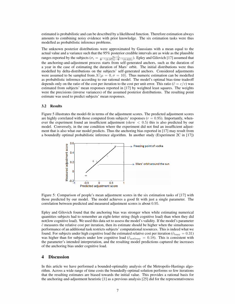
Figure 5 illustrates the model-fit in terms of the adjustment scores. The predicted adjustment scoresare highly correlated with those computed from subjects’ responses (r = 0.95). Importantly, when-ever the experiment found an insufficient adjustment (skew < 0.5) this is also predicted by ourmodel. Conversely, in the one condition where the experiment did not find an insufficient adjust-ment that is also what our model predicts. Thus the anchoring bias reported in [17] may result froma boundedly optimal probabilistic inference algorithm. In another study (Experiment 2C in [17])
Figure 5: Comparison of people’s mean adjustment scores in the six estimation tasks of [17] withthose predicted by our model. The model achieves a good fit with just a single parameter. Thecorrelation between predicted and measured adjustment scores is about 0.95.
Epley and Gilovich found that the anchoring bias was stronger when while estimating numericalquantities subjects had to remember an eight-letter string (high cognitive load) than when they didnot(low cognitive load). We used this data set to assess the model’s validity. If the model’s parameterc̃ measures the relative cost per iteration, then its estimate should be higher when the simultaneousperformance of an additional task restricts subjects’ computational resources. This is indeed what wefound. For subjects under high cognitive load the estimated relative cost per iteration (c̃busy = 0.31)was higher than for subjects under low cognitive load (c̃notbusy = 0.18). This is consistent withthe parameter’s intended interpretation, and the resulting model predictions captured the increasesof the anchoring bias under cognitive load.
4 Discussion
In this article we have performed a bounded-optimality analysis of the Metropolis-Hastings algo-rithm. Across a wide range of time costs the boundedly-optimal solution performs so few iterationsthat the resulting estimates are biased towards the initial value. This provides a rational basis forthe anchoring-and-adjustment heuristic [1] as a previous analysis [25] did for the representativeness
7

heuristic [1]. By deriving the anchoring-and-adjustment heuristic from a general approximate infer-ence algorithm we open the door to understanding how this heuristic should apply in domains morecomplex than the estimation of a single number. From previous work in psychology, it is not obviouswhat an adjustment should look like in the space of objects or events, for instance. By reinterpretingadjustment in terms of MCMC, we extend it to almost arbitrary domains of inference. Furthermoreour model illustrates that heuristics in general can be formalized by and derived as boundedly opti-mal approximations to rational inference. This provides a new perspective on the resulting cognitivebiases: the anchoring bias is tolerated because its consequences are less costly than the time thatwould be required to eliminate it. Thus the anchoring bias can be interpreted as a sign of boundedoptimality rather than irrationality. This may be equally true of other cognitive biases, because elim-inating bias can be costly and biased beliefs do not necessarily lead to poor decisions (see Figure4).
This article illustrates the value of bounded optimality as a framework for deriving models of cog-nitive processes. This approach is a formal synthesis of the function-first approach underlyingBayesian models of cognition [2] with the limitations-first approach that starts from cognitive andperceptual illusions (e.g. [1]). This synthesis can be achieved by augmenting the problems facingthe mind with constraints on information processing and solving them formally using optimization.Rather than determining optimal beliefs and actions, this approach seeks to determine boundedlyoptimal processes. Conversely, given a process the same framework can be used to determine theprocessing constraints under which it is boundedly optimal. This idea is so general that it can beapplied to reverse-engineering the whole spectrum of mental algorithms and processing constraints.
Understanding the mind’s probabilistic inference algorithm(s) will require many more steps than wehave been able to take so far. We have demonstrated the bounded-optimality of very few iterationsin a trivial inference problem for which an analytical solution exists. Thus, one may argue that ourconclusions could be specific to a simple one-dimensional inference problem. However, our resultsfollow from a very general mathematical property: the geometric convergence of the Metropolis-Hastings algorithm. This property is also true of many complex and high-dimensional inferenceproblems [18]. Furthermore, Equation 8 predicts that if the inference problem becomes more diffi-cult, then the bias b? tolerated by a boundedly-optimal MCMC algorithm increases, because highercomplexity leads to slower convergence and this means r → 1. This suggests, that resource-rationalsolutions to the challenging inference problems facing the human mind are likely to be biased, butthis remains to be shown. In addition, the solution determined by our bounded-optimality analysisremains to be evaluated against alternative solutions to real-time decision-making under uncertainty.Furthermore, while our model was consistent with existing data, our formalization of the estimationtask can be questioned, and since [17] did not report standard errors, we were unable to perform aproper statistical assessment of our model. It therefore remains to be shown whether or not people’sbias-time tradeoff is indeed near-optimal. This will require dedicated experiments that systemati-cally manipulate probability structure, time pressure, and error costs.
The prevalence of Bayesian computational-level models has made a sampling based view of mentalprocessing attractive—after all, sampling algorithms are flexible and efficient solutions to difficultBayesian inference problems. Vul et al. [7] explored the rational use of a sampling capacity, arguingthat it is often rational to decide based on only one perfect sample. However, perfect samples canbe hard to come by; here we have shown that it can be rational to decide based on one imperfectsample. A rational sampling-based view of mental processing thus leads naturally to a biased mind.
Acknowledgments. This work was supported by grant number FA-9550-10-1-0232 from the Air Force Officeof Scientific Research (Thomas L. Griffiths) and a John S. McDonnell Foundation Scholar Award (Noah D.Goodman).
References
[1] A. Tversky and D. Kahneman. Judgment under uncertainty: Heuristics and biases. Science,185(4157):1124–1131, 1974.
[2] T. L. Griffiths, C. Kemp, and J. B. Tenenbaum. Bayesian models of cognition. In R. Sun, editor,The Cambridge handbook of computational psychology, chapter 3, pages 59–100. CambridgeUniversity Press, 2008.
8

[3] D. Marr. Vision: A Computational Investigation into the Human Representation and Process-ing of Visual Information. W. H. Freeman, 1983.
[4] A. N. Sanborn, T. L. Griffiths, and D. J. Navarro. Rational approximations to rational models:Alternative algorithms for category learning. Psychological Review, 117(4):1144–1167, 2010.
[5] L. Shi, T. L. Griffiths, N. H. Feldman, and A. N. Sanborn. Exemplar models as a mechanismfor performing Bayesian inference. Psychonomic Bulletin & Review, 17(4):443–464, 2010.
[6] E. Bonawitz, S. Denison, A. Chen, A. Gopnik, and T. L. Griffiths. A simple sequential algo-rithm for approximating bayesian inference. Proceedings of the 33rd Annual Conference ofthe Cognitive Science Society, Austin, TX: Cognitive Science Society, 2011.
[7] E. Vul, N. D. Goodman, T. L. Griffiths, and J. B. Tenenbaum. One and done? Optimal decisionsfrom very few samples. Proceedings of the 31st Annual Conference of the Cognitive ScienceSociety, 2009.
[8] T. L. Griffiths and J. B. Tenenbaum. Optimal predictions in everyday cognition. PsychologicalScience, 17(9):767–773, 2006.
[9] T. L. Griffiths and J. B. Tenenbaum. Predicting the future as bayesian inference: People com-bine prior knowledge with observations when estimating duration and extent. Journal of Ex-perimental Psychology: General, 140(4):725–743, 2011.
[10] N.D. Goodman, J. B. Tenenbaum, J. Feldman, and T. L. Griffiths. A rational analysis of rule-based concept learning. Cognitive Science, 32(1):108–154, 2008.
[11] S. J. Gershman, E. Vul, and J. B. Tenenbaum. Multistability and perceptual inference. NeuralComputation, 24(1):1–24, 2011.
[12] R. Moreno-Bote, D. C. Knill, and A. Pouget. Bayesian sampling in visual perception. Pro-ceedings of the National Academy of Sciences, 108(30):12491–12496, 2011.
[13] L. Buesing, J. Bill, B. Nessler, and W. Maass. Neural dynamics as sampling: a model forstochastic computation in recurrent networks of spiking neurons. PLoS Computational Biol-ogy, 7(11):e1002211+, 2011.
[14] D. Pecevski, L. Buesing, and W. Maass. Probabilistic inference in general graphical modelsthrough sampling in stochastic networks of spiking neurons. PLoS Computational Biology,7(12):e1002294+, 2011.
[15] E. Horvitz. Reasoning about beliefs and actions under computational resource constraints. InUncertainty in Artificial Intelligence 3 Annual Conference on Uncertainty in Artificial Intelli-gence (UAI-87), pages 301–324, Amsterdam, NL, 1987. Elsevier Science.
[16] W. K. Hastings. Monte Carlo sampling methods using Markov chains and their applications.Biometrika, 57(1):97–109, 1970.
[17] N. Epley and T. Gilovich. The anchoring-and-adjustment heuristic. Psychological Science,17(4):311–318, 2006.
[18] K. L. Mengersen and R. L. Tweedie. Rates of convergence of the Hastings and Metropolisalgorithms. The Annals of Statistics, 24(1):101–121, 1996.
[19] A. E. Raftery and S. Lewis. How many iterations in the Gibbs sampler. In Bayesian Statistics4, volume 4, pages 763–773, 1992.
[20] N. Epley and T. Gilovich. When effortful thinking influences judgmental anchoring: differen-tial effects of forewarning and incentives on self-generated and externally provided anchors.Journal of Behavioral Decision Making, 18(3):199–212, 2005.
[21] N. Epley, B. Keysar, L. Van Boven, and T. Gilovich. Perspective taking as egocentric anchoringand adjustment. Journal of Personality and Social Psychology, 87(3):327–339, 2004.
[22] E. Vul and H. Pashler. Measuring the crowd within. Psychological Science, 19(7):645–647,2008.
[23] J. Huttenlocher, L. V. Hedges, and J. L. Vevea. Why do categories affect stimulus judgment?Journal of experimental psychology. General, 129(2):220–241, 2000.
[24] P. Hemmer and M. Steyvers. A Bayesian account of reconstructive memory. Topics in Cogni-tive Science, 1(1):189–202, 2009.
9

[25] J. B. Tenenbaum and T. L. Griffiths. The rational basis of representativeness. In Proceedingsof the 23rd Annual Conference of the Cognitive Science Society, pages 84–98, 2001.
10