business cycle dynamics under rational inattention · business cycle dynamics under rational...
TRANSCRIPT

WORK ING PAPER SER I E SNO 1331 / APR I L 2011
by Bartosz Maćkowiakand Mirko Wiederholt
BUSINESS CYCLE DYNAMICS UNDER RATIONAL INATTENTION

WORKING PAPER SER IESNO 1331 / APR I L 2011
BUSINESS CYCLE DYNAMICS
UNDER RATIONAL INATTENTION 1
by Bartosz Maćkowiak 2 and Mirko Wiederholt 3
1 We thank for helpful comments: Paco Buera, Larry Christiano, James Costain, Martin- Eichenbaum, Christian Hellwig, Marek Jarociński,
Giorgio Primiceri, Chris Sims, Bruno Strulovici, Andrea Tambalotti and seminar and conference participants at Amsterdam,
Bank of Canada, Bonn, Carlos III, Chicago Fed, Columbia, Cowles Foundation Summer Conference 2009, DePaul, Duke,
Einaudi Institute, European Central Bank, ESSIM 2008, EUI, Harvard, LSE, Madison, Mannheim, MIT,
Minneapolis Fed, Minnesota Workshop in Macroeconomic Theory 2009, NBER Summer
Institute 2008, NYU, NAWMES 2008, Philadelphia Fed, Pompeu Fabra, Princeton,
Richmond Fed, Riksbank, SED 2008, Stony Brook, Toronto, Toulouse, UCSD,
University of Chicago, University of Hong Kong, University of Montreal,
Wharton and Yale.
2 CEPR and European Central Bank, Kaiserstrasse 29, D-60311 Frankfurt am Main, Germany; e-mail: [email protected]
3 Department of Economics, Northwestern University, 2001 Sheridan Road, Evanston, IL 60208, USA;
e-mail: [email protected]
This paper can be downloaded without charge from http://www.ecb.europa.eu or from the Social Science Research Network electronic library at http://ssrn.com/abstract_id=1804852.
NOTE: This Working Paper should not be reported as representing the views of the European Central Bank (ECB). The views expressed are those of the authors
and do not necessarily reflect those of the ECB.In 2011 all ECB
publicationsfeature a motif
taken fromthe €100 banknote.
© European Central Bank, 2011
AddressKaiserstrasse 2960311 Frankfurt am Main, Germany
Postal addressPostfach 16 03 1960066 Frankfurt am Main, Germany
Telephone+49 69 1344 0
Internethttp://www.ecb.europa.eu
Fax+49 69 1344 6000
All rights reserved.
Any reproduction, publication and reprint in the form of a different publication, whether printed or produced electronically, in whole or in part, is permitted only with the explicit written authorisation of the ECB or the authors.
Information on all of the papers published in the ECB Working Paper Series can be found on the ECB’s website, http://www.ecb.europa.eu/pub/scientific/wps/date/html/index.en.html
ISSN 1725-2806 (online)

3ECB
Working Paper Series No 1331April 2011
Abstract 4
Non-technical summary 5
1 Introduction 7
2 Model setup 13
2.1 Households 13
2.2 Firms 14
2.3 Government 15
2.4 Shocks 16
2.5 Notation 17
3 Derivation of the fi rms’ objective 17
4 Derivation of the households’ objective 22
5 Aggregation 27
6 Solution under perfect information 28
7 Rational inattention by fi rms 30
7.1 The attention problem of the decision-maker in a fi rm 30
7.2 Computing the equilibrium of the model 34
7.3 Benchmark parameter values and solution 36
7.4 The effects of changes in parameter values 41
7.5 Extension: signals 43
8 Rational inattention by households and fi rms 47
8.1 The attention problem of a household 48
8.2 Computing the equilibrium of the model 52
8.3 Benchmark parameter values and solution 52
8.4 The effects of changes in parameter values 56
8.5 Extension: households set nominal wage rates 57
9 Conclusion 58
Appendix 59
References 61
Figures 65
CONTENTS
4ECBWorking Paper Series No 1331April 2011
Abstract
We develop a dynamic stochastic general equilibrium model with rational inattention by
households and rms. Consumption responds slowly to interest rate changes because households
decide to pay little attention to the real interest rate. Prices respond quickly to some shocks
and slowly to other shocks. The mix of fast and slow responses of prices to shocks matches the
pattern found in the empirical literature. Changes in the conduct of monetary policy yield very
di erent outcomes than in models currently used at central banks because systematic changes
in policy cause reallocation of attention by decision-makers in households and rms.
Keywords: information choice, rational inattention, monetary policy, business cycles. (JEL:
D83, E31, E32, E52).

5ECB
Working Paper Series No 1331April 2011
NON-TECHNICAL SUMMARY
The idea of rational inattention is that decision-makers have a limited amount of attention and decide how to allocate their attention. This paper develops a dynamic stochastic general equilibrium (DSGE) model with rational inattention by households and firms. We are motivated by the question of how to model the inertia found in macroeconomic data. Standard DSGE models used for policy analysis match this inertia by introducing multiple sources of slow adjustment: Calvo price setting, habit formation in consumption, Calvo wage setting, and other sources in richer models. We pursue the alternative idea that the inertia found in macroeconomic data can be understood as the result of one source of slow adjustment: rational inattention, that is, deliberate inattention by decision-makers as the outcome of a choice problem. Moreover, the degree of slow adjustment is endogenous because when the environment changes the allocation of attention changes.
We summarise the model’s predictions in four points. The first prediction of the model is that consumption responds very slowly to interest rate changes because households decide to pay little attention to movements in the real interest rate. This finding is important because in a large class of models monetary policy affects the real economy through the following channel. The central bank changes the nominal interest rate; due to some form of sticky prices the real interest rate changes; and households respond with their consumption to the change in the real interest rate. Our model predicts that the last part of this channel will be very slow, that is, the model predicts that consumption will respond very slowly to a change in the real interest rate. This is what the empirical literature finds. Moreover, our finding that households choose to pay little attention to movements in the real interest rate holds for low and high values of the coefficient of relative risk aversion.
The second prediction of the model is that prices respond quickly to some shocks and slowly to other shocks. The mix of quick and slow responses of prices to shocks matches the pattern found in the empirical literature. Specifically, the model predicts that prices respond very quickly to market-specific shocks, fairly quickly to aggregate technology shocks, and slowly to monetary policy shocks. The reason is the following. When we calibrate the model so as to match key features of the U.S. data like the large average absolute size of price changes in micro data and the small variance of the innovation in the Taylor rule, most of the variation in the profit-maximizing price is due to market-specific shocks, considerable variation in the profit-maximizing price is due to aggregate technology shocks, and little variation in the profit-maximizing price is due to monetary policy shocks. Decision-makers in firms who have to set prices thus pay close attention to market-specific conditions, some attention to aggregate technology, and little attention to monetary policy. Prices therefore respond very quickly to market-specific shocks, fairly quickly to aggregate technology shocks, and slowly to monetary policy shocks.
The third set of predictions of the model concern how households and firms interact in general equilibrium under rational inattention. To understand this interaction, we first solve the model with rational inattention by firms only and we then add rational inattention by households. We find that adding rational inattention by households has the following implications for aggregate dynamics. First, since households decide to pay little attention to movements in the real interest rate, the impulse response of
6ECBWorking Paper Series No 1331April 2011
consumption to a monetary policy shock becomes hump-shaped. Second, since consumption now responds less and more slowly to monetary policy shocks, decision-makers in firms choose to pay even less attention to monetary policy. Prices therefore respond even more slowly to monetary policy shocks. In summary, households’ optimal allocation of attention affects firms’ optimal allocation of attention.
The fourth prediction is that the outcomes of experiments in this DSGE model with rational inattention are very different than in DSGE models currently used for monetary policy analysis. Moreover, there is a clear intuition for why the outcomes are different: the allocation of attention varies with the economic environment. Consider an example. Since monetary policy is described by a Taylor rule (i.e., a policy rule stating that the nominal interest rate is a function of inflation and a measure of economic activity), one can ask the following question. What happens when the central bank fights inflation more aggressively? In other words, what happens when the central bank raises the interest rate more strongly in response to inflation? In the Calvo model, increasing the coefficient on inflation in the Taylor rule reduces the variance of the output gap, where the output gap is defined as the difference between output and the efficient level of output. This feature of the Calvo model is important, because this feature underlies the conventional wisdom that fighting inflation more aggressively moves the economy closer to the efficient level of output. By contrast, in the rational inattention model there is a non-monotonic relationship between the coefficient on inflation in the Taylor rule and the variance of the output gap. In our benchmark economy the following happens. When the central bank increases the coefficient on inflation in the Taylor rule, the variance of the output gap due to aggregate technology shocks first rises and then falls, and the variance of the output gap due to monetary policy shocks increases. The reason for the different outcomes is that in the rational inattention model there is an additional effect. When the central bank stabilizes the price level more, decision-makers in firms decide to pay less attention to aggregate conditions. As a result, the model yields an outcome that is very different from the conventional wisdom derived from DSGE models currently used at central banks.

7ECB
Working Paper Series No 1331April 2011
1 Introduction
Economists have studied for a long time how decision-makers allocate scarce resources. The recent
literature on rational inattention studies how decision-makers allocate the scarce resource attention.
The idea of rational inattention is that decision-makers have a limited amount of attention and
decide how to allocate their attention. This paper develops a dynamic stochastic general equilibrium
(DSGE) model with rational inattention by households and rms. Following Sims (2003), we model
limited attention as a constraint on information ow and we let decision-makers in households
and rms choose information ows subject to the constraint on information ow. For example,
consider a household that has to decide how much to consume and which goods to consume. To
take the optimal consumption-saving decision and to buy the optimal consumption basket, the
household has to know the real interest rate and the prices of all consumption goods. The idea of
rational inattention applied to this example is that: knowing the real interest rate and the prices
of all consumption goods requires attention; households have a limited amount of attention; and
households choose themselves how to allocate their attention. We study the implications of rational
inattention for business cycle dynamics.
We are motivated by the question of how to model the inertia found in macroeconomic data.
Standard DSGE models used for policy analysis match this inertia by introducing multiple sources
of slow adjustment: Calvo price setting, habit formation in consumption, Calvo wage setting,
and other sources in richer models.1 We pursue the alternative idea that the inertia found in
macroeconomic data can be understood as the result of one source of slow adjustment: rational
inattention, that is, deliberate inattention by decision-makers as the outcome of a choice problem.
Moreover, the degree of slow adjustment is endogenous because when the environment changes the
allocation of attention changes.
We model an economy with many households, many rms, and a government. Firms produce
di erentiated goods with a variety of types of labor. Households consume the variety of goods,
supply the di erentiated types of labor, and hold nominal government bonds. Firms take price
setting and labor mix decisions, while households take consumption and wage setting decisions.
The central bank sets the nominal interest rate according to a Taylor rule. The economy is a ected
by aggregate technology shocks, monetary policy shocks, and rm-speci c productivity shocks. The
1See, for example, Woodford (2003), Christiano, Eichenbaum and Evans (2005), and Smets and Wouters (2007).

8ECBWorking Paper Series No 1331April 2011
only source of slow adjustment is rational inattention by decision-makers in rms and households.
We compute the rational expectations equilibrium of the model.
We summarize the model’s predictions in four points. The rst prediction of the model is that
consumption responds very slowly to interest rate changes because households decide to pay little
attention to movements in the real interest rate. This nding is important because in a large class
of models monetary policy a ects the real economy through the following channel. The central
bank changes the nominal interest rate; due to some form of sticky prices the real interest rate
changes; and households respond with their consumption to the change in the real interest rate.
Our model predicts that the last part of this channel will be very slow, that is, the model predicts
that consumption will respond very slowly to a change in the real interest rate. This is what the
empirical literature nds.2 Moreover, our nding that households choose to pay little attention to
movements in the real interest rate holds for low and high values of the coe cient of relative risk
aversion. The reasons are the following. For low values of the coe cient of relative risk aversion,
deviations from the consumption Euler equation are cheap in utility terms. For high values of
the coe cient of relative risk aversion, the coe cient on the real interest rate in the consumption
Euler equation is small. This implies that households do not want to respond strongly to changes
in the real interest rate anyway. Therefore, for low and high values of the coe cient of relative
risk aversion, imperfect tracking of the real interest rate causes only small utility losses. Hence,
households decide to pay little attention to movements in the real interest rate.
The second prediction of the model is that prices respond quickly to some shocks and slowly to
other shocks. The mix of quick and slow responses of prices to shocks matches the pattern found in
the empirical literature. Speci cally, the model predicts that prices respond very quickly to market-
speci c shocks, fairly quickly to aggregate technology shocks, and slowly to monetary policy shocks.
The reason is the following. When we calibrate the model so as to match key features of the U.S.
2The literature on structural vector autoregressions nds that consumption shows a slow, hump-shaped response
to a monetary policy shock. See, for example, Leeper, Sims and Zha (1996). The literature on standard DSGE models
used for policy analysis nds that the t of those models to macroeconomic data is maximized when the degree of
habit formation in consumption is large. See, for example, Justiniano and Primiceri (2008). With a large degree of
habit formation, consumption responds very slowly to a change in the real interest rate. Our model suggests that the
observed slow response of consumption to the real interest rate is the outcome of a decision problem by households
with standard preferences.
9ECB
Working Paper Series No 1331April 2011
data like the large average absolute size of price changes in micro data and the small variance of
the innovation in the Taylor rule, most of the variation in the pro t-maximizing price is due to
market-speci c shocks, considerable variation in the pro t-maximizing price is due to aggregate
technology shocks, and little variation in the pro t-maximizing price is due to monetary policy
shocks. Decision-makers in rms who have to set prices thus pay close attention to market-speci c
conditions, some attention to aggregate technology, and little attention to monetary policy. Prices
therefore respond very quickly to market-speci c shocks, fairly quickly to aggregate technology
shocks, and slowly to monetary policy shocks. Interestingly, the empirical literature nds in the
data the same pattern of quick and slow responses of prices to shocks: Boivin, Giannoni and Mihov
(2009) and Mackowiak, Moench and Wiederholt (2009) nd that prices respond very quickly to
disaggregate shocks; Altig, Christiano, Eichenbaum and Linde (2005) nd that the price level
responds fairly quickly to aggregate technology shocks; and Christiano, Eichenbaum and Evans
(1999), Leeper, Sims and Zha (1996) and Uhlig (2005) nd that the price level responds slowly to
monetary policy shocks. This mix of quick and slow responses of prices to shocks is di cult to
match with DSGE models currently used for monetary policy analysis (e.g., the Calvo model). In
an earlier paper, we present a model of price setting under rational inattention by rms that yields
a quick response of prices to idiosyncratic shocks and a slow response of prices to aggregate shocks.3
One new insight here is that distinguishing between di erent types of aggregate shocks (aggregate
technology shocks and monetary policy shocks) yields di erential speeds of response of prices to
di erent aggregate shocks that are consistent with the empirical ndings cited above. Another
new insight here is that these di erential speeds of response of prices to shocks arise both when
decision-makers in rms pay attention to the driving exogenous processes and when decision-makers
in rms pay attention to endogenous variables like the price level, sales, and the wage bill.
In our model and in any other model with a price setting friction, rms experience pro t losses
due to deviations of the price from the pro t-maximizing price. One nice feature of our model is
that those pro t losses due to deviations of the price from the pro t-maximizing price are small.
For comparison, in our benchmark economy pro t losses due to deviations of the price from the
pro t-maximizing price are 30 times smaller than in the Calvo model that generates the same real
e ects of monetary policy shocks. The main reason is that in our model prices respond slowly to
3See Mackowiak and Wiederholt (2009).

10ECBWorking Paper Series No 1331April 2011
monetary policy shocks, but quickly to market-speci c and aggregate technology shocks. The other
reason is that under rational inattention deviations of the price from the pro t-maximizing price
are less likely to be extreme than in the Calvo model.
The third set of predictions of the model concern how households and rms interact in general
equilibrium under rational inattention. To understand this interaction, we rst solve the model with
rational inattention by rms only and we then add rational inattention by households. We nd that
adding rational inattention by households has the following implications for aggregate dynamics.
First, since households decide to pay little attention to movements in the real interest rate, the
impulse response of consumption to a monetary policy shock becomes hump-shaped. Second, since
consumption now responds less and more slowly to monetary policy shocks, decision-makers in
rms choose to pay even less attention to monetary policy. Prices therefore respond even more
slowly to monetary policy shocks. In summary, households’ optimal allocation of attention a ects
rms’ optimal allocation of attention.
The fourth set of predictions concern policy experiments. Changes in the conduct of monetary
policy yield very di erent outcomes in this DSGE model than in DSGE models currently used
at central banks. This is because systematic changes in policy cause reallocation of attention by
decision-makers in rms and households. Here we would like to highlight one important example.
Since monetary policy is described by a Taylor rule (i.e., a policy rule stating that the nominal
interest rate is a function of in ation and a measure of economic activity), one can ask the following
question. What happens when the central bank ghts in ation more aggressively? In other words,
what happens when the central bank raises the interest rate more strongly in response to in ation?
In the Calvo model, increasing the coe cient on in ation in the Taylor rule reduces the variance of
the output gap, where the output gap is de ned as the di erence between output and the e cient
level of output. This feature of the Calvo model is important, because this feature underlies the
conventional wisdom that ghting in ation more aggressively moves the economy closer to the
e cient level of output. By contrast, in the rational inattention model there is a non-monotonic
relationship between the coe cient on in ation in the Taylor rule and the variance of the output gap.
In our benchmark economy the following happens. When the central bank increases the coe cient
on in ation in the Taylor rule, the variance of the output gap due to aggregate technology shocks
rst rises and then falls, and the variance of the output gap due to monetary policy shocks increases.

11ECB
Working Paper Series No 1331April 2011
The reason for the di erent outcomes is that in the rational inattention model there is an additional
e ect. When the central bank stabilizes the price level more, decision-makers in rms decide to
pay less attention to aggregate conditions. As a result, the model yields an outcome that is very
di erent from the conventional wisdom derived from DSGE models currently used at central banks.
Other experiments also yield very di erent outcomes than in other DSGE models. Another
conventional wisdom derived from models currently used for monetary policy analysis is that raising
strategic complementarity in price setting increases real e ects of monetary policy shocks. A
common way to raise strategic complementarity in price setting is to make a rm’s marginal cost
curve more upward sloping in own output. See, for example, Altig, Christiano, Eichenbaum and
Linde (2005). When we raise strategic complementarity in price setting by making a rm’s marginal
cost curve more upward sloping in own output, we nd that, for reasonable parameter values, real
e ects of monetary policy shocks become smaller not larger. The reason is that in the rational
inattention model there is an additional e ect. When the marginal cost curve becomes more upward
sloping in own output, the cost of a price setting mistake of a given size increases. Decision-makers
in rms therefore decide to pay more attention to the price setting decision, implying that prices
respond faster to shocks. This additional e ect dominates for reasonable parameter values and thus
real e ects of monetary policy shocks become smaller not larger.
To recapitulate, the outcomes of experiments in this DSGE model with rational inattention are
very di erent than in DSGE models currently used for monetary policy analysis. Moreover, there
is a clear intuition for why the outcomes are di erent: the allocation of attention varies with the
economic environment.
This paper is related to the literature on rational inattention (e.g., Sims (2003, 2006), Luo
(2008), Mackowiak and Wiederholt (2009), Woodford (2009), Van Nieuwerburgh and Veldkamp
(2009, 2010), Kacperczyk, Van Nieuwerburgh and Veldkamp (2010), Matejka (2010) and Mondria
(2010)).4 There are two important di erences to the existing literature on rational inattention.
First, this paper develops the rst dynamic stochastic general equilibrium (DSGE) model with
rational inattention. Mackowiak and Wiederholt (2009) is an equilibrium model of price setting
under rational inattention by rms. The demand side of the economy is an exogenous process for
nominal spending. This means that one cannot study the allocation of attention by households,
4See Sims (2010) or Veldkamp (2010) for a review of the literature on rational inattention.

12ECBWorking Paper Series No 1331April 2011
one cannot study the interaction between households and rms, and one cannot conduct the kind
of monetary policy experiments that central banks are interested in (e.g., what happens when
the central bank ghts in ation more aggressively). Setting up and solving a DSGE model with
rational inattention is not trivial. One has to specify how agents with rational inattention interact
in markets. We suppose that in each market one side of the market chooses the price and the other
side of the market chooses the quantity. Furthermore, households’ optimal allocation of attention
a ects rms’ optimal allocation of attention, and vice versa. Computing the equilibrium of the
model therefore amounts to solving a non-trivial xed point problem. Paciello (2010) solves a
general equilibrium model with rational inattention by rms analytically. The main di erences are
that in his model households have perfect information and the model is static in the sense that:
(i) all exogenous processes are white noise processes, (ii) the price level instead of in ation appears
in the Taylor rule, and (iii) there is no lagged interest rate in the Taylor rule. Second, this paper
studies consumption by households with rational inattention when the real interest rate uctuates.
Sims (2003, 2006), Luo (2008) and Tutino (2009) also study consumption-saving decisions under
rational inattention but in these papers the real interest rate is constant. Therefore, the point that
households have little incentive to track movements in the real interest rate (for low and high values
of the coe cient of relative risk aversion) is not in those papers. This point is important because
in a large class of models monetary policy a ects the real economy through the following channel.
The central bank changes the nominal interest rate; due to some form of price stickiness the real
interest rate changes; and households respond with their consumption to the change in the real
interest rate. If this is indeed the channel through which monetary policy a ects the real economy,
then the attention that households devote to the real interest rate is crucial.
The paper is also related to the literature on business cycle models with imperfect information
(e.g., Lucas (1972), Woodford (2002), Mankiw and Reis (2002), Angeletos and La’O (2009a, 2009b)
and Lorenzoni (2009)). The main di erence to this literature is that in our model decision-makers
choose the information structure (i.e., the information structure is derived from an objective and
a set of constraints). This has two implications. First, the model gives an explanation for the
equilibrium information structure. Second, the model predicts how the equilibrium information
structure varies with policy. The fact that the equilibrium information structure varies with policy
has important implications for the outcome of policy experiments.

13ECB
Working Paper Series No 1331April 2011
The paper is organized as follows. Section 2 describes all features of the economy apart from the
attention problem of decision-makers. Sections 3 and 4 derive the objectives that decision-makers in
rms and households maximize when they decide how to allocate their attention. Section 5 discusses
aggregation. Section 6 presents the analytical solution of the model under perfect information.
Section 7 states the attention problem of the decision-maker in a rm and presents solutions of the
model with rational inattention by rms and perfect information by households. Section 8 states
the attention problem of a household and presents solutions of the model with rational inattention
by households and rms. Section 9 concludes.
2 Model setup
In this section we describe all features of the economy apart from information ows. Thereafter,
we solve the model for alternative assumptions about information ows: (i) perfect information,
(ii) rational inattention by rms, and (iii) rational inattention by households and rms.
In the model, there are three types of agents (households, rms and the government) and three
types of markets (goods markets, labor markets and a bond market). We suppose that in each
market one side of the market chooses the price and the other side of the market chooses the
quantity. In goods markets, rms set prices and households decide how much to buy. In labor
markets, households set wage rates and rms decide how much to hire. In the bond market, the
government sets the nominal interest rate and households decide how many bonds to hold.
2.1 Households
There are households in the economy. Households supply di erentiated types of labor, consume
a variety of goods, and hold nominal government bonds.
Time is discrete and households have an in nite horizon. Each household seeks to maximize
the expected discounted sum of period utility. The discount factor is (0 1). The period utility
function is
( ) =
1 1
1
1+
1 +(1)
where
=
ÃX=1
1
!1
(2)

14ECBWorking Paper Series No 1331April 2011
Here is composite consumption by household in period , is labor supply by household
in period , and is consumption of good by household in period . The parameter 0 is
the inverse of the intertemporal elasticity of substitution. The parameters 0 and 0 a ect
the disutility of supplying labor. There are di erent consumption goods and the parameter 1
is the elasticity of substitution between those consumption goods.5
The ow budget constraint of household in period reads
X=1
+ = 1 1 + (1 + ) + (3)
where is the price of good in period , are holdings of nominal government bonds by
household between period and period +1, is the nominal gross interest rate on those bond
holdings, is the nominal wage rate for labor supplied by household in period , is a wage
subsidy paid by the government, ( ) is a pro-rata share of nominal aggregate pro ts, and ( )
is a pro-rata share of nominal lump-sum taxes. We assume that all households have the same initial
bond holdings 1 0. We also assume that bond holdings have to be positive in every period,
0. We have to make some assumption to rule out Ponzi schemes. We choose this particular
assumption because it will allow us to express bond holdings in terms of log-deviations from the
non-stochastic steady state. One can think of households as having an account. The account holds
only nominal government bonds and the balance on the account has to be positive.
In every period, each household chooses a consumption vector, ( 1 ), and a wage rate.
Each household commits to supply any quantity of labor at that wage rate.
Each household takes as given: all prices of consumption goods, the nominal wage index de ned
below, the nominal interest rate, and all aggregate quantities.
2.2 Firms
There are rms in the economy. Firms supply di erentiated consumption goods.
Firm supplies good . The production function of rm is
= (4)
5The assumption of a constant elasticity of substitution between consumption goods is only for ease of exposition.
One could use a general constant returns-to-scale consumption aggregator.
15ECB
Working Paper Series No 1331April 2011
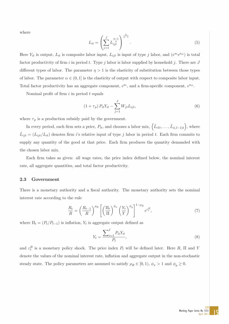
where
=X=1
11
(5)
Here is output, is composite labor input, is input of type labor, and ( ) is total
factor productivity of rm in period . Type labor is labor supplied by household . There are
di erent types of labor. The parameter 1 is the elasticity of substitution between those types
of labor. The parameter (0 1] is the elasticity of output with respect to composite labor input.
Total factor productivity has an aggregate component, , and a rm-speci c component, .
Nominal pro t of rm in period equals
(1 + )X=1
(6)
where is a production subsidy paid by the government.
In every period, each rm sets a price, , and chooses a labor mix,³ˆ1
ˆ( 1)
´, where
ˆ = ( ) denotes rm ’s relative input of type labor in period . Each rm commits to
supply any quantity of the good at that price. Each rm produces the quantity demanded with
the chosen labor mix.
Each rm takes as given: all wage rates, the price index de ned below, the nominal interest
rate, all aggregate quantities, and total factor productivity.
2.3 Government
There is a monetary authority and a scal authority. The monetary authority sets the nominal
interest rate according to the rule
=
μ1¶ "μ ¶ μ ¶ #1
(7)
where = ( 1) is in ation, is aggregate output de ned as
=
X=1 (8)
and is a monetary policy shock. The price index will be de ned later. Here , and
denote the values of the nominal interest rate, in ation and aggregate output in the non-stochastic
steady state. The policy parameters are assumed to satisfy [0 1), 1 and 0.

16ECBWorking Paper Series No 1331April 2011
The government budget constraint in period reads
+ = 1 1 +
ÃX=1
!+
X=1
(9)
The government has to nance maturing nominal government bonds, the production subsidy and
the wage subsidy. The government can collect lump-sum taxes or issue new government bonds.
We assume that the government sets the production subsidy, , and the wage subsidy, , so
as to correct the distortions arising from rms’ market power in the goods market and households’
market power in the labor market. In particular, we assume that
=˜
˜ 11 (10)
where ˜ denotes the price elasticity of demand, and
=˜
˜ 11 (11)
where ˜ denotes the wage elasticity of labor demand. We make this assumption to abstract from
the level distortions arising from monopolistic competition.6
2.4 Shocks
There are three types of shocks in the economy: aggregate technology shocks, rm-speci c produc-
tivity shocks, and monetary policy shocks. We assume that the stochastic processes { }, { 1 },{ 2 },..., { } and © ª
are independent. Furthermore, we assume that follows a stationary
Gaussian rst-order autoregressive process with mean zero, each follows a stationary Gaussian
rst-order autoregressive process with mean zero, and follows a Gaussian white noise process.
In the following, we denote the period innovation to and by and , respectively.
When we aggregate decisions by individual rms, the term 1X
=1appears. This term is a
random variable with mean zero and variance 1¡ ¢
. When we aggregate individual decisions,
we neglect this term because the term has mean zero and a variance that can be made small by
setting the number of rms equal to a large number. We work with a nite number of rms
because a household with rational inattention cannot track a continuum of prices.7
6When households have perfect information, the price elasticity of demand ˜ equals the preference parameter
. When households have imperfect information, the price elasticity of demand ˜ may di er from the preference
parameter . Hence, the value of the production subsidy (10) may vary across information structures.7Dixit and Stiglitz (1977) also assume that there is a nite number of rms and that rms take the price index

17ECB
Working Paper Series No 1331April 2011
2.5 Notation
In this subsection we introduce convenient notation. Throughout the paper, denotes aggregate
composite consumption
=X=1
(12)
and denotes aggregate composite labor input
=X=1
(13)
Furthermore, ˆ denotes the relative price of good
ˆ = (14)
and ˆ denotes the relative wage rate for type labor
ˆ = (15)
In addition, ˜ denotes the real wage rate for type labor
˜ = (16)
and ˜ denotes the real wage index
˜ = (17)
In each section we will specify the de nition of and .
3 Derivation of the rms’ objective
In this section we derive a log-quadratic approximation to expected pro ts. We use this expression
for expected pro ts below when we assume that decision-makers in rms choose the allocation of
their attention so as to maximize expected pro ts. To derive this expression, we proceed in four
steps: (i) we make a guess concerning the demand function for good , (ii) we derive the pro t
function of rm , (iii) we make an assumption about how decision-makers in rms value pro t
as given. Moreover, it seems a good description of the U.S. economy that there is a nite number of rms producing
consumption goods and that rms take the consumer price index (CPI) as given.
18ECBWorking Paper Series No 1331April 2011
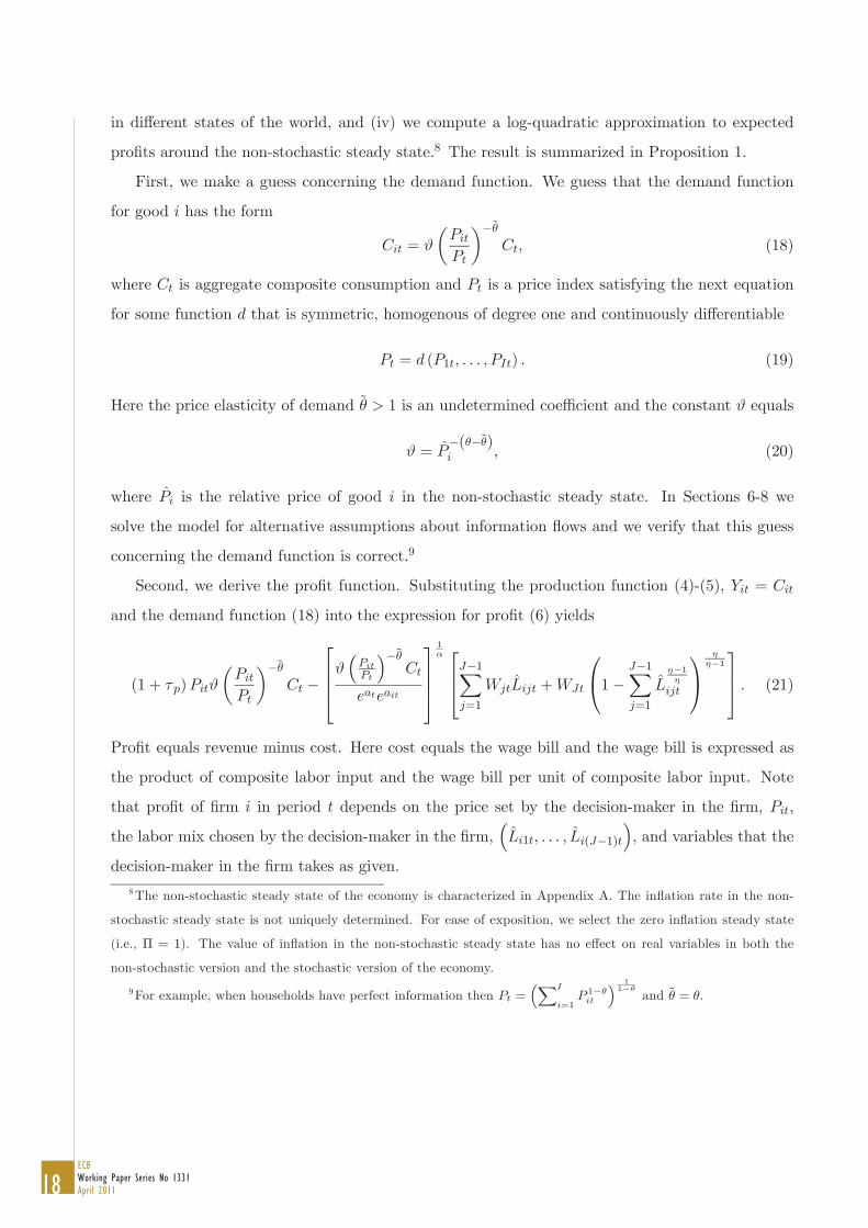
in di erent states of the world, and (iv) we compute a log-quadratic approximation to expected
pro ts around the non-stochastic steady state.8 The result is summarized in Proposition 1.
First, we make a guess concerning the demand function. We guess that the demand function
for good has the form
=
μ ¶ ˜
(18)
where is aggregate composite consumption and is a price index satisfying the next equation
for some function that is symmetric, homogenous of degree one and continuously di erentiable
= ( 1 ) (19)
Here the price elasticity of demand ˜ 1 is an undetermined coe cient and the constant equals
= ˆ ( ˜)(20)
where ˆ is the relative price of good in the non-stochastic steady state. In Sections 6-8 we
solve the model for alternative assumptions about information ows and we verify that this guess
concerning the demand function is correct.9
Second, we derive the pro t function. Substituting the production function (4)-(5), =
and the demand function (18) into the expression for pro t (6) yields
(1 + )
μ ¶ ˜³ ´ ˜
1
1X=1
ˆ + 11X
=1
ˆ1
1
(21)
Pro t equals revenue minus cost. Here cost equals the wage bill and the wage bill is expressed as
the product of composite labor input and the wage bill per unit of composite labor input. Note
that pro t of rm in period depends on the price set by the decision-maker in the rm, ,
the labor mix chosen by the decision-maker in the rm,³ˆ1
ˆ( 1)
´, and variables that the
decision-maker in the rm takes as given.
8The non-stochastic steady state of the economy is characterized in Appendix A. The in ation rate in the non-
stochastic steady state is not uniquely determined. For ease of exposition, we select the zero in ation steady state
(i.e., = 1). The value of in ation in the non-stochastic steady state has no e ect on real variables in both the
non-stochastic version and the stochastic version of the economy.
9For example, when households have perfect information then ==1
11
1and ˜ = .
19ECB
Working Paper Series No 1331April 2011
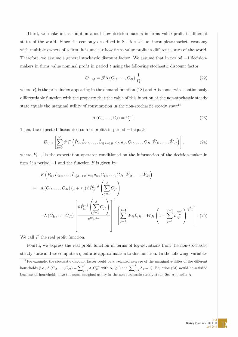
Third, we make an assumption about how decision-makers in rms value pro t in di erent
states of the world. Since the economy described in Section 2 is an incomplete-markets economy
with multiple owners of a rm, it is unclear how rms value pro t in di erent states of the world.
Therefore, we assume a general stochastic discount factor. We assume that in period 1 decision-
makers in rms value nominal pro t in period using the following stochastic discount factor
1 = ( 1 )1
(22)
where is the price index appearing in the demand function (18) and is some twice continuously
di erentiable function with the property that the value of this function at the non-stochastic steady
state equals the marginal utility of consumption in the non-stochastic steady state10
( 1 ) = (23)
Then, the expected discounted sum of pro ts in period 1 equals
1
"X=0
³ˆ ˆ
1ˆ( 1) 1
˜1
˜´#
(24)
where 1 is the expectation operator conditioned on the information of the decision-maker in
rm in period 1 and the function is given by³ˆ ˆ
1ˆ( 1) 1
˜1
˜´
= ( 1 ) (1 + ) ˆ1 ˜ X=1
( 1 )
ˆ ˜ X=1
1
1X=1
˜ ˆ + ˜ 11X
=1
ˆ1
1
(25)
We call the real pro t function.
Fourth, we express the real pro t function in terms of log-deviations from the non-stochastic
steady state and we compute a quadratic approximation to this function. In the following, variables10For example, the stochastic discount factor could be a weighted average of the marginal utilities of the di erent
households (i.e., ( 1 ) ==1
with 0 and=1
= 1). Equation (23) would be satis ed
because all households have the same marginal utility in the non-stochastic steady state. See Appendix A.
20ECBWorking Paper Series No 1331April 2011
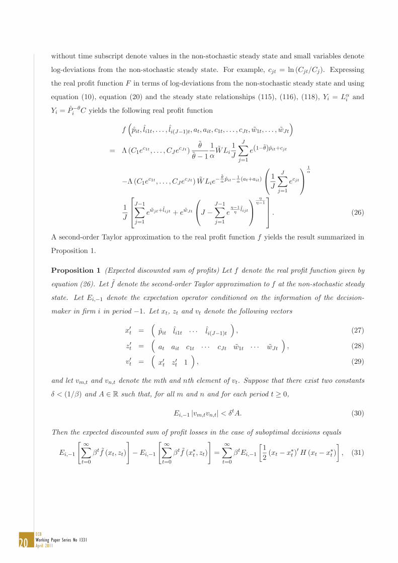
without time subscript denote values in the non-stochastic steady state and small variables denote
log-deviations from the non-stochastic steady state. For example, = ln ( ). Expressing
the real pro t function in terms of log-deviations from the non-stochastic steady state and using
equation (10), equation (20) and the steady state relationships (115), (116), (118), = and
= ˆ yields the following real pro t function³ˆ ˆ
1ˆ( 1) 1 ˜1 ˜
´= ( 1
1 )˜
˜ 1
1 ˜ 1X=1
(1 ˜)ˆ +
( 11 ) ˜
˜ˆ 1 ( + ) 1X
=1
1
11X
=1
˜ +ˆ + ˜1X
=1
1ˆ1
(26)
A second-order Taylor approximation to the real pro t function yields the result summarized in
Proposition 1.
Proposition 1 (Expected discounted sum of pro ts) Let denote the real pro t function given by
equation (26). Let ˜ denote the second-order Taylor approximation to at the non-stochastic steady
state. Let 1 denote the expectation operator conditioned on the information of the decision-
maker in rm in period 1. Let , and denote the following vectors
0 =³ˆ ˆ
1 · · · ˆ( 1)
´(27)
0 =³
1 · · · ˜1 · · · ˜´
(28)
0 =³
0 0 1´
(29)
and let and denote the th and th element of . Suppose that there exist two constants
(1 ) and R such that, for all and and for each period 0,
1 | | (30)
Then the expected discounted sum of pro t losses in the case of suboptimal decisions equals
1
"X=0
˜( )
#1
"X=0
˜( )
#=X=0
11
2( )0 ( )
¸(31)
21ECB
Working Paper Series No 1331April 2011
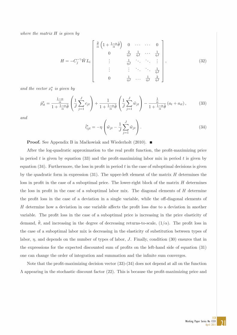
where the matrix is given by
= ˜
˜³1 + 1 ˜
´0 · · · · · · 0
0 2 1 · · · 1
... 1 . . . . . ....
......
. . . . . . 1
0 1 1 2
(32)
and the vector is given by
ˆ =1
1 + 1 ˜1X
=1
+1
1 + 1 ˜1X
=1
˜1
1 + 1 ˜( + ) (33)
and
ˆ = ˜1X
=1
˜ (34)
Proof. See Appendix B in Mackowiak and Wiederholt (2010).
After the log-quadratic approximation to the real pro t function, the pro t-maximizing price
in period is given by equation (33) and the pro t-maximizing labor mix in period is given by
equation (34). Furthermore, the loss in pro t in period in the case of suboptimal decisions is given
by the quadratic form in expression (31). The upper-left element of the matrix determines the
loss in pro t in the case of a suboptimal price. The lower-right block of the matrix determines
the loss in pro t in the case of a suboptimal labor mix. The diagonal elements of determine
the pro t loss in the case of a deviation in a single variable, while the o -diagonal elements of
determine how a deviation in one variable a ects the pro t loss due to a deviation in another
variable. The pro t loss in the case of a suboptimal price is increasing in the price elasticity of
demand, ˜, and increasing in the degree of decreasing returns-to-scale, (1 ). The pro t loss in
the case of a suboptimal labor mix is decreasing in the elasticity of substitution between types of
labor, , and depends on the number of types of labor, . Finally, condition (30) ensures that in
the expressions for the expected discounted sum of pro ts on the left-hand side of equation (31)
one can change the order of integration and summation and the in nite sum converges.
Note that the pro t-maximizing decision vector (33)-(34) does not depend at all on the function
appearing in the stochastic discount factor (22). This is because the pro t-maximizing price and

22ECBWorking Paper Series No 1331April 2011
labor mix are the solution to a static maximization problem. Furthermore, the expected discounted
sum of pro t losses (31) depends only on the value of the function at the non-stochastic steady
state. The reason is the log-quadratic approximation to the real pro t function around the non-
stochastic steady state.
Proposition 1 gives an expression for expected pro t losses in the case of suboptimal decisions
for the economy presented in Section 2 when the demand function is given by equation (18) and
the stochastic discount factor is given by equation (22). From this expression one can already
see to some extent how the decision-maker in a rm who cannot attend perfectly to all available
information will allocate his or her attention. For example, the attention devoted to the price
setting decision will depend on the loss in pro t in the case of a deviation of the price from the
pro t-maximizing price. Formally, the attention devoted to the price setting decision will depend
on the upper-left element of the matrix . Furthermore, for the decision-maker in a rm it is
particularly important to track those changes in the environment that in expectation cause most of
the uctuations in the pro t-maximizing decisions. As one can see from equations (33)-(34), which
changes in the environment in expectation cause most of the uctuations in the pro t-maximizing
decisions depends on the calibration of the exogenous processes, the technology parameters and ,
and the behavior of other agents in the economy. Namely, the price setting behavior of other rms
and the consumption and wage setting behavior of households will a ect the optimal allocation of
attention by the decision-maker in a rm.
4 Derivation of the households’ objective
In this section we derive a log-quadratic approximation to expected utility. We use this expression
for expected utility below when we assume that households choose the allocation of attention so as to
maximize expected utility. To derive this expression, we proceed in three steps: (i) we make a guess
concerning the demand function for type labor, (ii) we substitute the labor demand function, the
ow budget constraint, and the consumption aggregator into the period utility function to obtain
a period utility function that incorporates these constraints, and (iii) we compute a log-quadratic
approximation to expected utility around the non-stochastic steady state. The result is summarized
in Proposition 2.

23ECB
Working Paper Series No 1331April 2011
First, we make a guess concerning the labor demand function. We guess that the demand
function for type labor has the form
=
μ ¶ ˜
(35)
where is aggregate composite labor input and is a wage index satisfying the next equation
for some function that is symmetric, homogenous of degree one and continuously di erentiable
= ( 1 ) (36)
Here the wage elasticity of labor demand ˜ 1 is an undetermined coe cient and the constant
equals
= ˆ ( ˜) (37)
In Sections 6-8 we solve the model for alternative assumptions about information ows and we
verify that this guess concerning the labor demand function is correct.11
Second, we substitute the labor demand function, the ow budget constraint, and the consump-
tion aggregator into the period utility function to obtain a period utility function that incorporates
these constraints. Rearranging the ow budget constraint (3) yields
=1 1 + (1 + ) +X
=1ˆ
where ˆ = ( ) is relative consumption of good and the denominator on the right-hand
side is consumption expenditure per unit of composite consumption. Dividing the numerator and
the denominator on the right-hand side by some price index yields
=1 ˜
1˜ + (1 + ) ˜ +
˜ ˜X=1ˆ ˆ
(38)
where ˜ = ( ) are real bond holdings by the household, = ( 1) is in ation,
˜ = ( ) are real aggregate pro ts, and ˜ = ( ) are real lump-sum taxes. Furthermore,
rearranging the consumption aggregator (2) yields
1 =X=1
ˆ1
(39)
11For example, when rms have perfect information then ==1
11
1and ˜ = .

24ECBWorking Paper Series No 1331April 2011
Substituting the labor demand function (35), the ow budget constraint (38), and the consumption
aggregator (39) into the period utility function (1) yields a period utility function that incorporates
these constraints:
1
1
1 ˜1
˜ + (1 + ) ˜³˜
˜
´ ˜+
˜ ˜
1X=1
ˆ ˆ + ˆ
Ã1
1X=1
ˆ1
!1
1
1
1 1 +
Ø
˜
! ˜ 1+
(40)
Third, we express the period utility function (40) in terms of log-deviations from the non-
stochastic steady state and we compute a quadratic approximation to the expected discounted sum
of period utility around the non-stochastic steady state. Expressing the period utility function (40)
in terms of log-deviations from the non-stochastic steady state and using equation (11), equation
(37) and the steady state relationships (112)-(114), (117) and = ˆ yields the following
period utility function
1
1
1 +˜ 1˜+ ˜
˜ 1(1 ˜) ˜ +˜ ˜ + +
˜ ˜
11X
=1
ˆ +ˆ + 1 ˆ
Ã1X
=1
1 ˆ
!1
1
1
1
1
1 +˜(1+ )( ˜ ˜ )+(1+ ) (41)
where , , and denote the following steady state ratios³ ´=³
˜ ˜ ˜ ˜ ´(42)
A second-order Taylor approximation to the expected discounted sum of period utility yields the
result summarized in Proposition 2.
Proposition 2 (Expected discounted sum of period utility) Let denote the functional that is
obtained by multiplying the period utility function (41) by and summing over all from zero to
in nity. Let ˜ denote the second-order Taylor approximation to at the non-stochastic steady state.

25ECB
Working Paper Series No 1331April 2011
Let 1 denote the expectation operator conditioned on information of household in period 1.
Let , and denote the following vectors
0 =³˜ ˜ 1 · · · ˆ 1
´(43)
0 =³
1 ˜ ˜ ˜ 1 · · · ˆ´
(44)
0 =³
0 0 1´
(45)
and let and denote the th and th element of . Suppose that
1
h˜2
1
i(46)
and for all ,
1
¯˜
1 0
¯(47)
Suppose also that there exist two constants (1 ) and R such that, for all and , for
each period 0, and for = 0 1,
1 | + | (48)
Then the expected discounted sum of utility losses in the case of suboptimal decisions equals
1
h˜³˜
1 0 0 1 1
´i1
h˜³˜
1 0 0 1 1
´i=
X=0
11
2( )0 0 ( ) + ( )0 1
¡+1 +1
¢¸(49)
Here the matrix 0 equals
0 =1
2³1 + 1
´˜ 0 · · · 0
˜ ˜ ( ˜ + 1 + ˜) 0 · · · 0
0 0 2 · · · 1
......
.... . .
...
0 0 1 · · · 2
(50)
the matrix 1 equals
1 =1
2 ˜ 0 · · · 0
0 0 0 · · · 0
0 0 0 · · · 0...
....... . .
...
0 0 0 · · · 0
(51)
26ECBWorking Paper Series No 1331April 2011
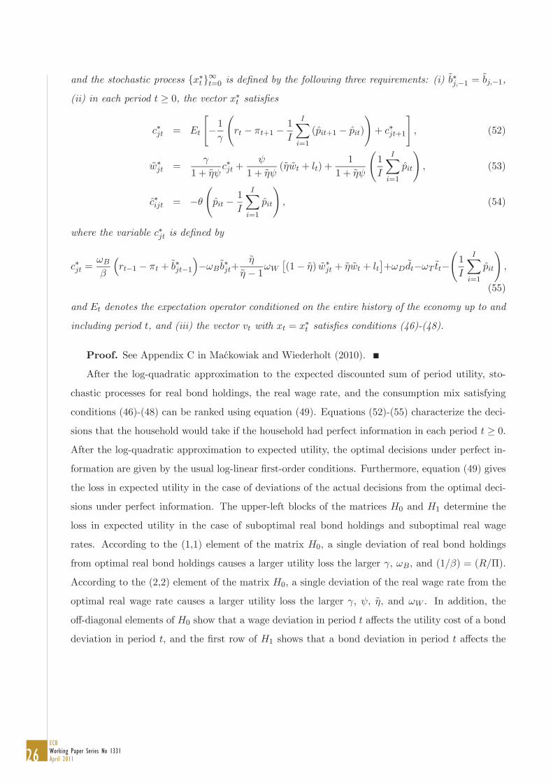
and the stochastic process { } =0 is de ned by the following three requirements: (i) ˜ 1 =˜
1,
(ii) in each period 0, the vector satis es
=
"1Ã
+11X
=1
(ˆ +1 ˆ )
!+ +1
#(52)
˜ =1 + ˜
+1 + ˜
(˜ ˜ + ) +1
1 + ˜
Ã1X
=1
ˆ
!(53)
ˆ =
È
1X=1
ˆ
!(54)
where the variable is de ned by
=³
1 +˜ 1
´˜ +
˜
˜ 1
£(1 ˜) ˜ + ˜ ˜ +
¤+ ˜ ˜
Ã1X
=1
ˆ
!(55)
and denotes the expectation operator conditioned on the entire history of the economy up to and
including period , and (iii) the vector with = satis es conditions (46)-(48).
Proof. See Appendix C in Mackowiak and Wiederholt (2010).
After the log-quadratic approximation to the expected discounted sum of period utility, sto-
chastic processes for real bond holdings, the real wage rate, and the consumption mix satisfying
conditions (46)-(48) can be ranked using equation (49). Equations (52)-(55) characterize the deci-
sions that the household would take if the household had perfect information in each period 0.
After the log-quadratic approximation to expected utility, the optimal decisions under perfect in-
formation are given by the usual log-linear rst-order conditions. Furthermore, equation (49) gives
the loss in expected utility in the case of deviations of the actual decisions from the optimal deci-
sions under perfect information. The upper-left blocks of the matrices 0 and 1 determine the
loss in expected utility in the case of suboptimal real bond holdings and suboptimal real wage
rates. According to the (1,1) element of the matrix 0, a single deviation of real bond holdings
from optimal real bond holdings causes a larger utility loss the larger , , and (1 ) = ( ).
According to the (2,2) element of the matrix 0, a single deviation of the real wage rate from the
optimal real wage rate causes a larger utility loss the larger , , ˜, and . In addition, the
o -diagonal elements of 0 show that a wage deviation in period a ects the utility cost of a bond
deviation in period , and the rst row of 1 shows that a bond deviation in period a ects the

27ECB
Working Paper Series No 1331April 2011
utility cost of a bond deviation in period + 1 and the utility cost of a wage deviation in period
+1. The lower-right block of the matrix 0 determines the loss in expected utility in the case of a
suboptimal consumption mix. The loss in expected utility in the case of a suboptimal consumption
mix is decreasing in the elasticity of substitution between consumption goods, , and depends on
the number of consumption goods, . Finally, conditions (46)-(48) ensure that in the expressions
for the expected discounted sum of period utility on the left-hand side of equation (49) one can
change the order of integration and summation and all in nite sums converge.
Proposition 2 gives an expression for the expected discounted sum of utility losses in the case of
deviations of the actual decisions from the optimal decisions under perfect information for the econ-
omy presented in Section 2 when the labor demand function is given by equation (35). Proposition
2 is important because inattention leads to deviations of the actual decisions from the decisions that
the household would take under perfect information. To choose the optimal allocation of attention,
the household has to compare the cost in terms of expected utility of di erent types of deviations
from the optimal decisions under perfect information. From Proposition 2 one can already see to
some extent how parameters a ect the optimal allocation of attention by a household. For example,
consider the role of . Increasing raises the utility loss in the case of a given deviation of real
bond holdings from optimal real bond holdings. At the same time, increasing lowers the response
of optimal real bond holdings to the real interest rate. The relative strength of these two e ects
determines whether for a household with a higher it is more or less important to be aware of
movements in the real interest rate.
5 Aggregation
In this section we describe issues related to aggregation. In the following, we work with log-
linearized equations for aggregate variables. Log-linearizing the equations for aggregate output (8),
aggregate composite consumption (12), and aggregate composite labor input (13) yields
=1X
=1
(ˆ + ) (56)
=1X
=1
(57)

28ECBWorking Paper Series No 1331April 2011
and
=1X
=1
(58)
Log-linearizing the equations for the price index (19) and the wage index (36) yields
0 =X=1
ˆ (59)
and
0 =X=1
ˆ (60)
The last two equations can be stated as
=1X
=1
(61)
and
=1X
=1
(62)
Furthermore, we work with log-linearized equations when we aggregate the demand for a par-
ticular consumption good or for a particular type of labor. Formally,
=1X
=1
(63)
and
=1X
=1
(64)
Note that the production function (4) and the Taylor rule (7) are already log-linear:
= + + (65)
and
= 1 + (1 )¡
+¢+ (66)
6 Solution under perfect information
In this section we present the solution of the model under perfect information as a benchmark.
We de ne the equilibrium of the model under perfect information as follows. In each period , all
29ECB
Working Paper Series No 1331April 2011
agents know the entire history of the economy up to and including period . Firms choose the pro t-
maximizing price and labor mix, households choose the utility-maximizing consumption vector and
wage rate, and the government sets the nominal interest rate according to the Taylor rule, sets the
subsidies according to equations (10)-(11) and follows a Ricardian scal policy. Finally, aggregate
variables are given by their respective equations and households have rational expectations.
The following proposition characterizes real variables at the solution of the model under perfect
information after the log-quadratic approximation to the real pro t function (see Section 3), the
log-quadratic approximation to the expected discounted sum of period utility (see Section 4), and
the log-linearization of the equations for the aggregate variables (see Section 5).
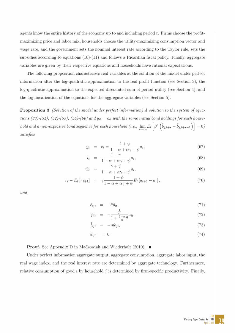
Proposition 3 (Solution of the model under perfect information) A solution to the system of equa-
tions (33)-(34), (52)-(55), (56)-(66) and = with the same initial bond holdings for each house-
hold and a non-explosive bond sequence for each household (i.e., limh ³
˜+
˜+ 1
´i= 0)
satis es
= =1 +
1 + +(67)
=1
1 + +(68)
˜ =+
1 + +(69)
[ +1] =1 +
1 + +[ +1 ] (70)
and
ˆ = ˆ (71)
ˆ =1
1 + 1 (72)
ˆ = ˆ (73)
ˆ = 0 (74)
Proof. See Appendix D in Mackowiak and Wiederholt (2010).
Under perfect information aggregate output, aggregate consumption, aggregate labor input, the
real wage index, and the real interest rate are determined by aggregate technology. Furthermore,
relative consumption of good by household is determined by rm-speci c productivity. Finally,

30ECBWorking Paper Series No 1331April 2011
rm ’s relative input of type labor is constant. Note that in this model under perfect information
monetary policy has no e ect on real variables. Monetary policy does a ect nominal variables. The
nominal interest rate and in ation follow from the Taylor rule (66) and the real interest rate (70).
Since (1 ) 0 and (1 ) + 1, the equilibrium paths of the nominal interest rate
and in ation are locally determinate.12
7 Rational inattention by rms
In this section we solve the model with rational inattention by decision-makers in rms and perfect
information by households. We maintain the assumption that households have perfect information
for the moment to isolate the implications of rational inattention by decision-makers in rms.
7.1 The attention problem of the decision-maker in a rm
Following Sims (2003), we model attention as an information ow and limited attention as a con-
straint on information ow. Decision-makers choose information ows, subject to the constraint on
information ow.
To take decisions that are close to the pro t-maximizing decisions, agents in rms have to be
aware of changes in the environment that cause changes in the pro t-maximizing decisions. Being
aware of changes in the environment requires information ow when these changes are stochastic.
A decision-maker in a rm with limited attention faces a trade-o : Tracking closely particular
changes in the environment improves decision making but also uses up valuable information ow.
We formalize this trade-o by letting decision-makers in rms choose directly the process for the
decision vector, subject to the constraint on information ow. For example, the decision-maker in
a rm can decide to respond swiftly and correctly with the price of the good to changes in rm-
speci c productivity but this requires allocating attention to rm-speci c productivity. We assume
that decision-makers in rms choose the allocation of attention so as to maximize the expected
discounted sum of pro ts net of the cost of attention. We interpret the cost of attention as an
opportunity cost.
12See Woodford (2003), Chapter 2, Proposition 2.8.

31ECB
Working Paper Series No 1331April 2011
Formally, the attention problem of the decision-maker in rm reads:
max1( ) 2( ) 3( ) 1( ) 2( ) 3( ) ˜
(X=0
11
2( )0 ( )
¸1
)(75)
where
=ˆ1
...
ˆ( 1)
ˆ1
...
ˆ( 1)
(76)
subject to the equations characterizing the pro t-maximizing decisions
= 1 ( )| {z }+ 2 ( )| {z }+ 3 ( )| {z } (77)
ˆ = ˆ (78)
the equations characterizing the actual decisions
= 1 ( ) + 1 ( )| {z }+ 2 ( ) + 2 ( )| {z }+ 3 ( ) + 3 ( )| {z } (79)
ˆ = ˜
μˆ +
( ˆ )
(80)
and the constraint on information ow
I³n
ˆ1
ˆ( 1)
o;n
ˆ1
ˆ( 1)
o´(81)
Here 1 ( ) to 3 ( ), 1 ( ) to 3 ( ), and 1 ( ) to 3 ( ) are in nite-order lag polynomials.
The noise terms , , , and in the actual decisions are assumed to follow Gaussian white
noise processes with unit variance that are: (i) independent of all other stochastic processes in
the economy, (ii) rm-speci c, and (iii) independent of each other. The operator I measures theamount of information that the actual decisions contain about the pro t-maximizing decisions.
This operator is de ned below. Finally, 1 in objective (75) denotes the expectation operator
conditioned on the information of the decision-maker in rm in period 1.
The objective (75) states that decision-makers in rms aim to maximize the expected discounted
sum of pro ts net of the cost of information ow. The rst term in curly brackets is the expected

32ECBWorking Paper Series No 1331April 2011
discounted sum of pro t losses in the case of deviations of the actual decisions from the pro t-
maximizing decisions. This term equals the right-hand side of equation (31) in Proposition 1.13
The second term in curly brackets is the cost of information ow. The parameter 0 is the
per-period marginal cost of information ow. We interpret this cost as an opportunity cost (i.e.,
devoting more attention to the price setting decision or the labor mix decision requires paying less
attention to some other decision of the rm that we do not model). The variable 0 is the total
information ow devoted to the price setting decision and the labor mix decision.
Equations (77)-(78) characterize the pro t-maximizing decisions. We guess that the pro t-
maximizing price (33) given in Proposition 1 has the representation (77) after substituting in
ˆ = , equations (57) and (62), and the equilibrium law of motion for , , ˜ , , and .
The guess will be veri ed. The pro t-maximizing labor mix (34) given in Proposition 1 reduces to
equation (78) after substituting in ˆ = ˜ ˜ and equation (62).
Equations (79)-(80) characterize the actual decisions. Consider rst equation (79). By choosing
the lag polynomials 1 ( ) and 1 ( ) to 3 ( ) and 3 ( ), the decision-maker chooses the stochas-
tic process for the price. For example, if the decision-maker chooses 1 ( ) = 1 ( ), 1 ( ) = 0,
2 ( ) = 2 ( ), 2 ( ) = 0, 3 ( ) = 3 ( ) and 3 ( ) = 0, the decision-maker decides to set
the actual price equal to the pro t-maximizing price in each period. The basic trade-o is the
following. Choosing a process for the actual price that tracks more closely the pro t-maximizing
price reduces pro t losses due to suboptimal price setting decisions but requires more attention.
Next, consider equation (80). By choosing the coe cients ˜ and , the decision-maker chooses the
wage elasticity of labor demand and the signal-to-noise ratio in the labor mix decision. The basic
trade-o is the following. When the pro t-maximizing labor mix is stochastic, choosing a process
for the actual labor mix that tracks more closely the pro t-maximizing labor mix reduces pro t
losses due to suboptimal hiring decisions but requires more attention.14
Finally, the information ow constraint (81) states that actual decisions containing more infor-
mation about the optimal decisions under perfect information require a larger information ow.
13 In equation (76), we use the fact that ˆ ˆ =14We put more structure on the labor mix decision than on the price setting decision by expressing the labor mix
as a function of relative wages rather than fundamental shocks. We do this because from equation (80) we derive
the labor demand function and a labor demand function speci es labor demand on and o the equilibrium path. By
expressing the labor mix as a function of relative wages, we specify labor demand on and o the equilibrium path.

33ECB
Working Paper Series No 1331April 2011
We follow Sims (2003) and a large literature in information theory by quantifying information
as reduction in uncertainty, where uncertainty is measured by entropy. Entropy is simply a measure
of uncertainty. The entropy of a normally distributed random vector = ( 1 ) equals
( ) =1
2log2
h(2 ) det
iwhere det is the determinant of the covariance matrix of . Conditional entropy is a measure
of conditional uncertainty. If the random vectors = ( 1 ) and = ( 1 ) have a
multivariate normal distribution, the conditional entropy of given knowledge of equals
( | ) = 1
2log2
h(2 ) det |
iwhere | is the conditional covariance matrix of given . Equipped with measures of un-
certainty and conditional uncertainty, one can quantify the information that the random vector
contains about the random vector as reduction in uncertainty, ( ) ( | ). The operatorI in the information ow constraint (81) is de ned as
I ({ } ; { }) = lim1[ ( 0 1) ( 0 1| 0 1)] (82)
where { } =0 and { } =0 are stochastic processes. The operator I quanti es the informationthat one process contains about another process by measuring the average per-period amount of
information that the rst elements of one process contain about the rst elements of the other
process and by letting go to in nity. If { } =0 is a stationary Gaussian process, then
I ({ } ; { }) = lim1 1
2log2
μdet
det |
¶¸(83)
If is a scalar then is the covariance matrix of the vector ( 0 1). If is itself a vector
then is the covariance matrix of the vector obtained by stacking the vectors 0 1.15
To complete the description of the decision problem (75)-(81), we have to specify the expectation
operator 1 in objective (75). We assume that 1 is the unconditional expectation operator.
Note that we have assumed that the actual decisions follow a Gaussian process. One can show
that a Gaussian process for the actual decisions is optimal because objective (75) is quadratic
15 If a variable appearing in the information ow constraint (81) is non-stationary, we replace the original variable
by its rst di erence on the left-hand side of (81) to ensure that entropy is always nite. Replacing a stationary
variable by its rst di erence on the left-hand side of (81) has no e ect on information ow.

34ECBWorking Paper Series No 1331April 2011
and the pro t-maximizing decisions (77)-(78) follow a Gaussian process.16 Furthermore, we have
assumed that the noise in the actual decisions is rm-speci c. This assumption accords well with
the idea that the friction is the limited attention of an individual decision-maker rather than the
public availability of information. Finally, we have assumed that the noise terms , , , and
are independent of each other. This assumption captures the idea that attending to aggregate
technology, attending to monetary policy, attending to rm-speci c productivity, and attending to
relative wage rates are independent activities. We relax this assumption in Section 7.5.
Two remarks are in place before we present solutions of the decision problem (75)-(81). When
we solve the decision problem (75)-(81) numerically, we turn this in nite-dimensional problem into
a nite-dimensional problem by parameterizing each in nite-order lag polynomial 1 ( ) to 3 ( )
and 1 ( ) to 3 ( ) as a lag-polynomial of an ARMA(p,q) process where and are nite.17
Furthermore, we evaluate the right-hand side of equation (83) for a very large but nite .
7.2 Computing the equilibrium of the model
We use an iterative procedure to solve for the rational expectations equilibrium of the model with
rational inattention by decision-makers in rms and perfect information by households. First, we
make a guess concerning the stochastic process for the pro t-maximizing price (77) and a guess
concerning the stochastic process for the relative wage rate in equation (78). Second, we solve
the rms’ attention problem (75)-(81). Third, we aggregate the individual prices to obtain the
aggregate price level
=1X
=1
(84)
Fourth, we compute the aggregate dynamics implied by those price level dynamics. The households’
optimality conditions (52)-(54) given in Proposition 2, equations (56)-(66), = , and the
assumption that aggregate technology follows a rst-order autoregressive process imply that the
following equations have to be satis ed in equilibrium:
=1( +1 + ) + +1
¸(85)
16See Sims (2006) or Section VIIA in Mackowiak and Wiederholt (2009).17We set = 2 and = 2, because we found that increasing or further failed to change noticeably the solution.
We allow the ARMA(p,q) process to have a unit root.
35ECB
Working Paper Series No 1331April 2011
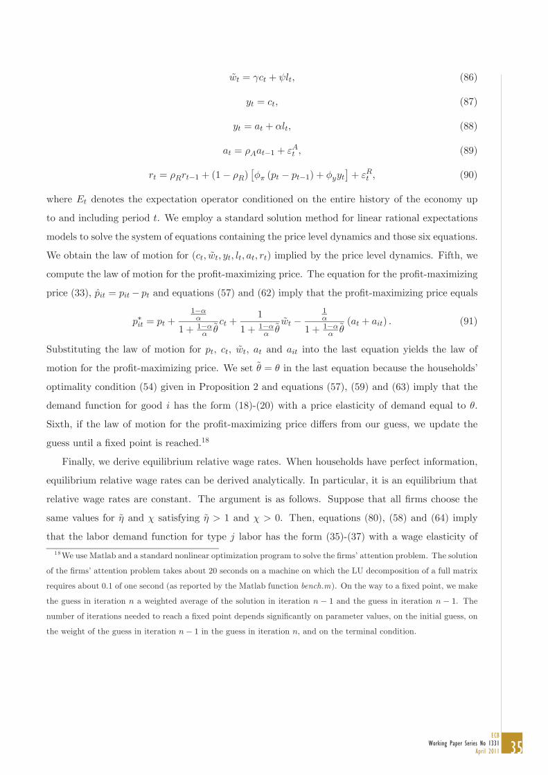
˜ = + (86)
= (87)
= + (88)
= 1 + (89)
= 1 + (1 )£
( 1) +¤+ (90)
where denotes the expectation operator conditioned on the entire history of the economy up
to and including period . We employ a standard solution method for linear rational expectations
models to solve the system of equations containing the price level dynamics and those six equations.
We obtain the law of motion for ( ˜ ) implied by the price level dynamics. Fifth, we
compute the law of motion for the pro t-maximizing price. The equation for the pro t-maximizing
price (33), ˆ = and equations (57) and (62) imply that the pro t-maximizing price equals
= +1
1 + 1 ˜+
1
1 + 1 ˜˜
1
1 + 1 ˜( + ) (91)
Substituting the law of motion for , , ˜ , and into the last equation yields the law of
motion for the pro t-maximizing price. We set ˜ = in the last equation because the households’
optimality condition (54) given in Proposition 2 and equations (57), (59) and (63) imply that the
demand function for good has the form (18)-(20) with a price elasticity of demand equal to .
Sixth, if the law of motion for the pro t-maximizing price di ers from our guess, we update the
guess until a xed point is reached.18
Finally, we derive equilibrium relative wage rates. When households have perfect information,
equilibrium relative wage rates can be derived analytically. In particular, it is an equilibrium that
relative wage rates are constant. The argument is as follows. Suppose that all rms choose the
same values for ˜ and satisfying ˜ 1 and 0. Then, equations (80), (58) and (64) imply
that the labor demand function for type labor has the form (35)-(37) with a wage elasticity of
18We use Matlab and a standard nonlinear optimization program to solve the rms’ attention problem. The solution
of the rms’ attention problem takes about 20 seconds on a machine on which the LU decomposition of a full matrix
requires about 0.1 of one second (as reported by the Matlab function bench.m). On the way to a xed point, we make
the guess in iteration a weighted average of the solution in iteration 1 and the guess in iteration 1. The
number of iterations needed to reach a xed point depends signi cantly on parameter values, on the initial guess, on
the weight of the guess in iteration 1 in the guess in iteration , and on the terminal condition.

36ECBWorking Paper Series No 1331April 2011
labor demand that is the same for all types of labor. Since all households face the same decision
problem and have the same information, all households set the same wage rate. Equation (62)
then implies that relative wage rates are constant ( ˆ = = 0). When relative wage rates
are constant, the pro t-maximizing labor mix is constant, implying that each rm can attain the
pro t-maximizing labor mix without any information ow. Since each rm can attain the pro t-
maximizing labor mix without any information ow, no rm has an incentive to deviate from the
chosen values for ˜ and .
7.3 Benchmark parameter values and solution
Next we report the numerical solution of the model for the following parameter values. One period
in the model is one quarter. We set = 0 99, = 1, = 0, = 4, = 2 3, and = 4.
To set the parameters of the rst-order autoregressive process for aggregate technology, we
consider quarterly U.S. data from 1960 Q1 to 2006 Q4 and we use equations (88)-(89). We rst
compute a time series for aggregate technology, , using equation (88) and measures of and .
We use the log of real output per person, detrended with a linear trend, as a measure of . We
use the log of hours worked per person, demeaned, as a measure of .19 We then t equation (89)
to the time series for obtaining = 0 96 and a standard deviation of the innovation equal to
0.0085. In the benchmark economy, we set = 0 95 and the standard deviation of equal to
0.0085.
To set the parameters of the monetary policy rule, we estimate the Taylor rule (90) with the
quarterly U.S. data on the Federal Funds rate, in ation, and real GDP from 1960 Q1 to 2006 Q4.
We obtain = 0 89, = 1 53, = 0 33, and a standard deviation of the innovation equal to
0.0021.20 In the benchmark economy, we set = 0 9, = 1 5, = 0 33, and the standard
19We use data for the non-farm business sector. The data source is the website of the Federal Reserve Bank of St.
Louis.20The speci cation of the monetary policy rule that we estimate is standard in the empirical literature on the
Taylor rule with partial adjustment. See, for example, Section 2 in Rudebusch (2002) for a review of this literature.
We regress a measure of the nominal interest rate on its own lag, a measure of the in ation rate, and a measure of the
output gap. The nominal interest rate is measured as the quarterly average Federal Funds rate. The in ation rate is
measured as 14
3=0 , where = ln ln 1 and is the price index for personal consumption expenditures
excluding food and energy. The output gap is measured as ( ) , where is real GDP and is potential
real GDP estimated by the Congressional Budget O ce. The data sources are the website of the Federal Reserve

37ECB
Working Paper Series No 1331April 2011
deviation of equal to 0.0021.21
To set the parameters of the rst-order autoregressive process for rm-speci c productivity,
we follow the recent literature calibrating menu cost models with rm-speci c productivity shocks
to U.S. micro price data. Nakamura and Steinsson (2008) and Bils, Klenow and Malin (2009)
set the autocorrelation of rm-speci c productivity in their monthly models equal to 0.66 and 0.7,
respectively. We set the autocorrelation of rm-speci c productivity equal to 0.3 because our model
is quarterly not monthly and (0 3)1 3 equals a number between 0.66 and 0.7. Furthermore, Klenow
and Kryvtsov (2008) report that the median absolute size of price changes (excluding sale-related
price changes) equals 9.7 percent in the U.S. We set the standard deviation of the innovation to
rm-speci c productivity such that the median absolute size of price changes equals 9.7 percent in
our model. This choice yields a standard deviation of the innovation to rm-speci c productivity
equal to 0.18.22
We compute the solution of the model by xing the marginal cost of information ow, 0.
The total information ow devoted to the price setting decision and the labor mix decision (i.e.,
) is endogenous. We interpret the marginal cost of information ow as an opportunity cost (i.e.,
the extra attention devoted to the price setting decision or the labor mix decision could have been
devoted to some other decision of the rm that we do not model). We set the marginal cost of
information ow equal to 0.1 percent of the rm’s steady state revenue. In objective (75) we value
this cost using the value of the stochastic discount factor at the non-stochastic steady state. This
yields = (0 001) (1 + ) ˆ . This value for the marginal cost of attention implies that in
equilibrium the expected per-period loss in pro t due to deviations of the actual price from the
Bank of St. Louis and the website of the Congressional Budget O ce. Note that in the empirical monetary policy
rule we measure the in ation rate as the four-quarter moving average of in ation rates. We do so following Section
2 in Rudebusch (2002). Using only the current in ation rate in the empirical monetary policy rule yields essentially
identical estimates.21We investigated the role of all parameters in the model. We report the e ects of changes in parameter values
in Section 7.4. Note that restricting the sample to the Great Moderation would have yielded a smaller standard
deviation of the innovation in the Taylor rule. In the model this would imply less attention to monetary policy
compared with the benchmark economy.22Note that we match the average size of price changes excluding sale-related price changes. If we were to match
the average size of all price changes, the standard deviation of the innovation to rm-speci c productivity would be
even larger.
38ECBWorking Paper Series No 1331April 2011
pro t-maximizing price equals 0.15 percent of the rm’s steady state revenue: (0 0015) (1 + ) ˆ .
We nd this number reasonable.23
We rst report the optimal allocation of attention at the equilibrium with rational inattention
by decision-makers in rms. Decision-makers in rms who have to set prices decide to pay most
attention to rm-speci c productivity, quite a bit of attention to aggregate technology, and little
attention to monetary policy. More precisely, of the total attention devoted to the price setting
decision, 65 percent is allocated to rm-speci c productivity, 26 percent is allocated to aggregate
technology, and 9 percent is allocated to monetary policy. Therefore, prices respond very quickly
to market-speci c shocks, fairly quickly to aggregate technology shocks, and slowly to monetary
policy shocks. The empirical literature nds in the data the same mix of quick and slow responses
of prices to shocks. Furthermore, for our value of the marginal cost of information ow, the total
attention devoted to the price setting decision is su ciently high so that the actual price set by
a rm tracks the pro t-maximizing price very well. The expected per-period loss in pro t due to
deviations of the actual price from the pro t-maximizing price equals 0.15 percent of the rm’s
steady state revenue.24 As we will point out below, this number for the expected loss in pro t
due to deviations of the actual price from the pro t-maximizing price is 30 times smaller than in
the Calvo model that yields the same responses of the price level and output to monetary policy
shocks.
Figures 1 and 2 show impulse responses of the price level, in ation, output, and the nominal
interest rate at the equilibrium with rational inattention by decision-makers in rms and perfect
information by households (green lines with circles). For comparison, the gures also include
impulse responses of the same variables at the equilibrium under perfect information derived in
Section 6 (blue lines with points). All impulse responses are to shocks of one standard deviation.
A response equal to one means a one percent deviation from the non-stochastic steady state. Time
23To illustrate this number, consider the following example. Suppose that the rm with a rationally inattentive
decision-maker has a pro t margin of 15 percent. If the decision-maker of the rm set the pro t-maximizing price in
each period, the pro t margin would increase to 15.15 percent. Hence, if one part of the decision-maker’s compensation
is proportional to the pro t margin, this part of the decision-maker’s compensation would increase by (1/100).24The expected per-period pro t loss due to imperfect tracking of rm-speci c productivity equals 0.07 percent of
the rm’s steady state revenue. The expected per-period pro t loss due to imperfect tracking of aggregate technology
equals 0.05 percent of the rm’s steady state revenue. The expected per-period pro t loss due to imperfect tracking
of monetary policy equals 0.03 percent of the rm’s steady state revenue.

39ECB
Working Paper Series No 1331April 2011
is measured in quarters along horizontal axes.
Consider Figure 1. Under rational inattention by decision-makers in rms, the price level shows
a dampened and delayed response to a monetary policy shock (compared with the case of perfect
information). The response of in ation to a monetary policy shock is persistent. Since the price
level responds slowly to a monetary policy shock, the real interest rate increases after a positive
innovation in the Taylor rule, implying that consumption and output fall. The fall in output is
persistent. The nominal interest rate increases on impact of a monetary policy shock and then
converges slowly to zero. By contrast, under perfect information by rms and households, the price
level adjusts fully on impact of a monetary policy shock, there are no real e ects, and the nominal
interest rate fails to change.
Consider Figure 2. The response of the price level to aggregate technology shocks is to some
extent dampened and delayed (compared with the case of perfect information). Therefore, output
is below perfect-information output for a few quarters after a positive aggregate technology shock,
implying that output shows a hump-shaped impulse response to an aggregate technology shock.
However, the response of the price level to aggregate technology shocks is stronger and faster than
the response of the price level to monetary policy shocks. The reason is that decision-makers in
rms decide to pay about three times as much attention to aggregate technology than to monetary
policy.25
Figure 3 shows the impulse response of an individual price to a rm-speci c productivity shock.
Prices respond very quickly to rm-speci c productivity shocks. The reason is that decision-makers
in rms decide to pay close attention to rm-speci c productivity.
Figures 1-3 show that the model matches the following three empirical ndings: (i) the model
matches the empirical nding by Boivin, Giannoni and Mihov (2009) and Mackowiak, Moench
and Wiederholt (2009) that prices respond very quickly to disaggregate shocks, (ii) the model
matches the empirical nding by Altig, Christiano, Eichenbaum and Linde (2005) that the price
level responds faster to aggregate technology shocks than to monetary policy shocks, and (iii)
the model matches the empirical nding that the price level responds slowly to monetary policy
shocks.26 The model matches this mix of very quick, fairly quick and slow responses of prices to
25The di erence between the response of the price level to monetary policy shocks and the response of the price level
to aggregate technology shocks becomes even more pronounced once we introduce rational inattention by households.26A number of di erent identi cation assumptions lead to the nding that the price level responds slowly to

40ECBWorking Paper Series No 1331April 2011
shocks with an endogenous allocation of attention. The reason is the following. When we calibrate
the model so as to match key features of the U.S. data like the large average absolute size of
price changes in micro data and the small standard deviation of the innovation in the Taylor rule,
most of the variation in the pro t-maximizing price is due to market-speci c shocks, considerable
variation in the pro t-maximizing price is due to aggregate technology shocks, and little variation
in the pro t-maximizing price is due to monetary policy shocks. Decision-makers in rms who are
responsible for setting prices therefore pay close attention to market-speci c conditions, quite a bit
of attention to aggregate technology, and little attention to monetary policy.27
For comparison, we solved the Calvo model with the same preference, technology, and mone-
tary policy parameters. The motivation for this comparison is that the Calvo model is the most
commonly used model for monetary policy analysis. We set the Calvo parameter so that prices
in the Calvo model change every 2.5 quarters on average because then the impulse responses to a
monetary policy shock are essentially identical in the Calvo model with perfect information and
in our benchmark economy with rational inattention by decision-makers in rms. See Figure 4.
While the impulse responses to a monetary policy shock are essentially identical in the two models,
the impulse responses to an aggregate technology shock are very di erent in the two models. See
Figure 5. The response of the price level to an aggregate technology shock is stronger and faster
in the benchmark economy than in the Calvo model, implying that output deviates from the e -
cient level of output for only 5 quarters in our benchmark economy while output deviates from the
e cient level of output for more than 20 quarters in the Calvo model. Hence, after an aggregate
technology shock, the rational inattention model is much closer to a frictionless economy than the
Calvo model. Furthermore, after a rm-speci c productivity shock, the rational inattention model
behaves essentially like a frictionless economy while there are large distortions in the Calvo model.
In the benchmark economy and in the Calvo model, rms experience pro t losses due to de-
viations of the actual price from the pro t-maximizing price. In the benchmark economy, the
expected loss in pro t due to deviations of the actual price from the pro t-maximizing price is 30
monetary policy shocks. See, for example, Christiano, Eichenbaum and Evans (1999), Leeper, Sims and Zha (1996),
and Uhlig (2005).27There is also the ampli cation e ect highlighted in Mackowiak and Wiederholt (2009) and Hellwig and Veldkamp
(2009). If other rms pay little attention to say monetary policy, the pro t-maximizing price moves less in response
to a monetary policy shock, which reduces the incentive for an individual rm to pay attention to monetary policy.

41ECB
Working Paper Series No 1331April 2011
times smaller than in the Calvo model that yields the same impulse responses of the price level and
output to a monetary policy shock.28 The main reason is that in the benchmark economy prices
respond slowly to monetary policy shocks, but fairly quickly to aggregate technology shocks and
very quickly to market-speci c shocks. The other reason is that in the rational inattention model
deviations of the actual price from the pro t-maximizing price are less likely to be extreme than in
the Calvo model.
7.4 The e ects of changes in parameter values
We now study whether the model yields di erent counterfactuals than other DSGE models (e.g.,
the Calvo model, a model with exogenous dispersed information, or the sticky information model).
Does it matter whether one uses this model or another DSGE model for policy analysis? We
conduct standard experiments like increasing the coe cient on in ation in the Taylor rule and
raising strategic complementarity in price setting. We nd that the outcomes of experiments
conducted with this model are very di erent from the outcomes of the same experiments conducted
with other DSGE models. The reason is that the allocation of attention is endogenous.
For example, let us vary the coe cient on in ation in the Taylor rule. Figure 6 shows the e ect
of increasing from 1.05 to 1.5 (our benchmark value) and then to 10 on the volatility of the output
gap.29 We report the standard deviation of the output gap due to aggregate technology shocks and
the standard deviation of the output gap due to monetary policy shocks. As increases in the
rational inattention model, the standard deviation of the output gap due to aggregate technology
shocks rst rises, peaking at 1.75, and then falls. The standard deviation of the output gap due
to monetary policy shocks is essentially constant until 1.75 and then rises. For comparison, as
increases in the Calvo model, the standard deviation of the output gap due to aggregate technology
shocks declines monotonically and the standard deviation of the output gap due to monetary
policy shocks declines monotonically. Hence, the rational inattention model yields a very di erent
28The expected loss in pro t due to suboptimal price responses to aggregate conditions is about 20 times smaller
than in the Calvo model. The expected loss in pro t due to suboptimal price responses to idiosyncratic conditions is
about 40 times smaller than in the Calvo model.29We de ne the output gap as the deviation of aggregate output from equilibrium aggregate output under perfect
information given in Proposition 3. Due to the subsidies (10)-(11), equilibrium aggregate output under perfect
information also equals e cient aggregate output.
42ECBWorking Paper Series No 1331April 2011
answer to the basic policy question of what happens when the central bank ghts in ation more
aggressively.
To understand how the value of a ects the economy in the two models, note the following.
As increases in the Calvo model, the nominal interest rate mimics more closely the real interest
rate at the e cient solution. This e ect reduces deviations of output from the e cient solution.
In the rational inattention model, there is an additional e ect. When the central bank responds
more aggressively with the nominal interest rate to in ation, the price level becomes more stable,
implying that decision-makers in rms decide to pay less attention to aggregate conditions. This
e ect increases deviations of output from the e cient solution. When the second e ect dominates
the rst e ect, the volatility of the output gap increases. For aggregate technology shocks the
second e ect dominates for values of below 1.75, while for monetary policy shocks the second
e ect dominates for values of above 1.75.
Second, consider raising strategic complementarity in price setting. There is a large literature
arguing that raising strategic complementarity in price setting increases real e ects of monetary
policy shocks. For example, Woodford (2003, Chapter 3) makes this point for the Calvo model and
Woodford (2002) makes this point for a model with exogenous dispersed information. A common
way to raise strategic complementarity in price setting is to make a rm’s marginal cost curve more
upward sloping in own output. See, for example, Altig, Christiano, Eichenbaum and Linde (2005).
We therefore consider the experiment of making a rm’s marginal cost curve more upward sloping
in own output. In particular, we raise the degree of decreasing returns-to-scale, (1 ). When we
decrease from 1 to 2/3 (our benchmark value) and then to 1/2, real e ects of monetary policy
shocks rst increase and then decrease. The reason is that there are two e ects. The rst e ect
is the e ect emphasized in the literature cited above. In the benchmark economy, a decrease in
lowers the coe cient on consumption in the equation for the pro t-maximizing price. Formally,
substituting equations (86)-(88) and ˜ = into equation (91) yields the following equation for the
pro t-maximizing price
= +1 + +
1 + 1
+ 1
1 + 1
1
1 + 1 (92)
A decrease in lowers the coe cient on consumption in equation (92) so long as ( + ) (1 + )
which is a parameter restriction that is satis ed in the benchmark economy. In the language of
Woodford (2003), a decrease in raises the degree of strategic complementarity in price setting.

43ECB
Working Paper Series No 1331April 2011
In the language of Ball and Romer (1990), a decrease in raises the degree of real rigidity. This
e ect increases real e ects of monetary policy shocks. However, in the rational inattention model,
there is an additional e ect. As decreases, the cost of a price setting mistake of a given size
increases. Formally, the upper-left element of the matrix in Proposition 1 increases in absolute
value. Decision-makers in rms therefore decide to pay more attention to the price setting decision,
implying that prices respond faster to shocks. This e ect reduces real e ects of monetary policy
shocks. We nd that the second e ect (more attention) dominates the rst e ect (lower coe cient
on consumption in the equation for the pro t-maximizing price) for values of below 2/3. Hence,
for reasonable parameter values, raising strategic complementarity reduces real e ects.
Third, consider increasing the variance of monetary policy shocks. In the rational inattention
model, decision-makers in rms decide to pay more attention to monetary policy, implying that
prices respond faster to monetary policy shocks and real e ects of a monetary policy shock of a
given size decrease. In the Calvo model, increasing the variance of monetary policy shocks has
no e ect on the responses of prices and output to a monetary policy shock of a given size. The
reallocation of attention in the rational inattention model is important quantitatively. For example,
in the benchmark economy, doubling the standard deviation of monetary policy shocks implies that
real e ects of monetary policy shocks last only 4 quarters instead of 10 quarters.
We could present the outcomes of many more experiments. The point is: the outcomes of
experiments are very di erent than in DSGE models currently used at central banks. Moreover,
there is a clear intuition for why the outcomes are so di erent: the allocation of attention varies
with the economic environment.
7.5 Extension: Signals
In this subsection we state the attention problem of the decision-maker in a rm using signals. We
also relax the assumption that attending to aggregate technology, attending to monetary policy,
and attending to rm-speci c productivity are independent activities.
We now assume that, in period 1, the decision-maker in a rm chooses the precision of the
signals that he or she will receive in the following periods. In each period 0, the decision-maker
receives the signals and takes the optimal price setting and labor mix decision given the signals. The
decision-maker chooses the precision of the signals in period 1 so as to maximize the expected
44ECBWorking Paper Series No 1331April 2011
discounted sum of pro ts net of the cost of information ow. The decision-maker understands
that a more precise signal will lead to better decision making but will also require more attention.
Formally, the attention problem of the decision-maker in rm reads:
max( 1 2 3 4) R5
+
(X=0
11
2( )0 ( )
¸1
)(93)
where
=ˆ1
...
ˆ( 1)
ˆ1
...
ˆ( 1)
(94)
subject to equations (77)-(78) characterizing the pro t-maximizing decisions, the following equation
characterizing the optimal decisions in period given information in period
= [ |F 0 1 2 ] (95)
the following equation characterizing the signal vector in period
=ˆ1...
ˆ( 1)
+
1
2
3
4 1
...
4 ( 1)
(96)
and the constraint on information ow
I³n
ˆ1
ˆ( 1)
o; { }
´(97)
The noise terms , , , and 1 to ( 1) in the signal are assumed to follow Gaussian white
noise processes with unit variance that are: (i) independent of all other stochastic processes in the
economy, (ii) rm-speci c, and (iii) independent of each other. As in the decision problem (75)-
(81), 1 in objective (93) denotes the expectation operator conditioned on the information of the
decision-maker in rm in period 1, the parameter 0 in objective (93) is the marginal cost of
information ow, and the operator I in the information ow constraint (97) is de ned by equation
45ECB
Working Paper Series No 1331April 2011
(82). We assume that 1 is the unconditional expectation operator. Finally, F 0 in equation
(95) denotes the information set of the decision-maker in rm in period zero. To abstract from
transitional dynamics in conditional second moments, we assume that in period zero (i.e., after the
decision-maker has chosen the precision of the signals in period 1), the decision-maker receives
information such that the conditional covariance matrix of given information in period is
constant for all 0.
We solve the problem (93)-(97) for an individual rm assuming that aggregate variables and
relative wage rates are given by the equilibrium of the benchmark economy presented in Section 7.3.
In other words, we assume that the behavior of all other rms and all households is given by the
benchmark economy presented in Section 7.3. We then compare the solution of problem (93)-(97)
to the solution of problem (75)-(81). Consider the left column of Figure 7. The blue lines with
points show the impulse responses of the pro t-maximizing price to the three fundamental shocks at
the equilibrium presented in Section 7.3. The green lines with circles show the impulse responses of
the price set by the rm to the three fundamental shocks when the rm solves problem (75)-(81).
The red lines with crosses show the impulse responses of the price set by the rm to the three
fundamental shocks when the rm solves problem (93)-(97). The decision problems (75)-(81) and
(93)-(97) yield the same price setting behavior: the green lines with circles and the red lines with
crosses in Figure 7 are identical, and the impulse responses of the price set by the rm to the noise
terms in equation (79) and to the noise terms in equation (96) also turn out to be identical.30,31
30We solve problem (93)-(97) numerically using Matlab and a standard nonlinear optimization program. We rst
approximate each of the following four objects by an ARMA(p,q) process where and are nite: the component of
driven by aggregate technology shocks, the component of driven by monetary policy shocks, the component of
driven by aggregate technology shocks, and the component of driven by monetary policy shocks. Then, there
exists a state-space representation of the dynamics of the signal (96) with a nite-dimensional state vector. We use
the Kalman lter to evaluate objective (93) and constraint (97) for any given choice of the precision of the signals.
We employ the program k lter.m, written by Lars Ljungqvist and Thomas J. Sargent, to solve for the conditional
covariance matrix of the state vector. Solving the problem (93)-(97) takes about as much time as solving the problem
(75)-(81). See Footnote 18. Below we also present solutions of problem (93)-(97) with the signal vector (98) instead
of the signal vector (96). Solving that problem turned out to be much more time-consuming. Here we had to evaluate
objective (93) and constraint (97) on a grid. Standard nonlinear optimization programs proved unhelpful because
numerical inaccuracy in the solution for the conditional covariance matrix of the state vector led to spurious variation
in the values of the objective and the constraint.31This is a numerical result. We were surprised that signals with noise that is i.i.d. across time yield the same

46ECBWorking Paper Series No 1331April 2011
We now relax the assumption that paying attention to aggregate technology, paying attention
to monetary policy, and paying attention to rm-speci c productivity are independent activities.
We replace the signal vector (96) by the following signal vector
=
+
1
1 + 1
ˆ1...
ˆ( 1)
+
1 1
2 2
3 3
4 4
5 1
...
5 ( 1)
(98)
By choosing 1 to 5 the decision-maker decides how much attention to devote to the price level,
total factor productivity, last period sales, the last period wage bill, and the relative wage rates.32,33
The variables in the signal vector (98) are driven by multiple shocks and it is therefore no longer
the case that attending to aggregate technology, attending to monetary policy, and attending to
rm-speci c productivity are independent activities. We nd that solving the problem (93)-(97)
with the signal vector (98) instead of the signal vector (96) changes the rm’s price setting behavior
hardly at all. See the right column of Figure 7. The price set by the rm responds somewhat faster
to aggregate technology shocks and somewhat slower to monetary policy shocks. Overall the red
lines with crosses in the right column of Figure 7 are very similar to the red lines with crosses
in the left column of Figure 7. The reason is that the decision-maker in the rm decides to pay
close attention to those variables that are mainly driven by rm-speci c productivity shocks and
aggregate technology shocks.
We studied a large number of variations of the signal vector (98) and obtained similar results.
First, we added other aggregate variables one by one to the signal vector. We found little or
price setting behavior as the more exible decision problem (75)-(81).32We maintain the assumption that the noise terms follow unit variance Gaussian white noise processes that are:
(i) independent of all other stochastic processes in the economy, (ii) rm-speci c, and (iii) independent of each other.33We include last period sales and last period wage bill in the signal vector because we do not know how the rm
can attend to current period sales and current period wage bill before setting the price. Below, when we do assume
that the rm can attend to current period sales and current period wage bill, we mean that the rm can attend to
the components of current period sales and current period wage bill that are independent of the own price, that is,
+ and + (1 ) ( + ), respectively.

47ECB
Working Paper Series No 1331April 2011
no e ect on the price setting behavior because the decision-maker of the rm decided to set the
precision of the additional signal to a small number or zero. Second, we replaced last period sales
and last period wage bill by current period sales and current period wage bill in the signal vector.
The price set by the rm then responds somewhat faster to aggregate technology shocks and to
monetary policy shocks, but the price still responds faster to aggregate technology shocks than to
monetary policy shocks. Third, we added rm-speci c demand shocks to the model by modifying
the consumption aggregator (2). We kept constant the variance of the rm-speci c component of
the pro t-maximizing price. We split this variance equally between rm-speci c productivity shocks
and rm-speci c demand shocks. We assumed the same persistence in rm-speci c productivity
and rm-speci c demand. We then solved again the decision problem (93)-(97) with the signal
vector (98). We found that adding rm-speci c demand shocks had almost no e ect on the impulse
responses of the price set by the rm to the other shocks. We obtained impulse responses that were
almost identical to the red lines with crosses in the right column of Figure 7.34
8 Rational inattention by households and rms
In this section we solve the model with rational inattention by households and rms.
To exhibit in the most transparent way the implications of rational inattention by households
for the intertemporal consumption decision, we make two assumptions in Sections 8.1-8.4. First,
we continue to assume that households have linear disutility of labor. Then the equation for the
optimal real wage rate, stating that the real wage rate should equal the marginal rate of substitution
between consumption and leisure, reduces to
˜ = (99)
where ˜ is the real wage rate for type labor and is composite consumption by household .
Second, we assume that households set real wage rates. Then households choose all variables in34Hellwig and Venkateswaran (2009) also study a model in which rms set prices in period based on signals
concerning sales and wage bills up to and including period 1. There are several di erences. First, in their
benchmark model the price level and total factor productivity are not included in the signal vector. More importantly,
in their model the noise in the signal is exogenous, whereas in our model the noise in the signal (98) is chosen optimally
subject to the constraint on information ow (97). In other words, they report impulse responses for some exogenously
given precision of the signals, whereas we report impulse responses for the optimal precision of the signals.
48ECBWorking Paper Series No 1331April 2011
the intratemporal optimality condition (99). Therefore, households will satisfy this intratemporal
optimality condition both under perfect information and under rational inattention. This allows us
to exhibit in the most transparent way the implications of rational inattention by households for
the intertemporal consumption decision. In Section 8.5, we also present the solution of the model
when households set nominal wage rates.35
8.1 The attention problem of a household
The attention problem of household in period 1 reads:
max1( ) 2( ) 1( ) 2( ) ˜
X=0
1
£12 ( )0 0 ( ) + ( )0 1
¡+1 +1
¢¤1
(100)
where
=
˜
˜
1
...
ˆ 1
˜
˜
1
...
ˆ 1
(101)
subject to the following equation linking an argument of the objective and two decision variables
˜ ˜ =X=0
μ1
1 £¡ ¢+ ˜
¡˜ ˜
¢¤(102)
the equations characterizing the optimal decisions under perfect information
= 1 ( )| {z }+ 2 ( )| {z } (103)
˜ = (104)
ˆ = ˆ (105)
35 In Sections 6-7 it did not matter whether households set real or nominal wage rates since households had perfect
information.
49ECB
Working Paper Series No 1331April 2011
the equations characterizing the actual decisions
= 1 ( ) + 1 ( )| {z }+ 2 ( ) + 2 ( )| {z } (106)
˜ = (107)
ˆ = ˜μˆ +
(ˆ )
(108)
and the constraint on information ow
I ¡© 1 ˆ 1
ª;©
1 ˆ 1
ª¢(109)
Here 1 ( ), 2 ( ), 1 ( ), 2 ( ), 1 ( ) and 2 ( ) are in nite-order lag polynomials. The noise
terms , and in the actual decisions are assumed to follow Gaussian white noise processes
with unit variance that are: (i) independent of all other stochastic processes in the economy,
(ii) household-speci c, and (iii) independent of each other. The operator I, de ned in equation(83), measures the amount of information that the household’s actual decisions contain about the
household’s optimal decisions under perfect information. Finally, 1 in objective (100) is the
expectation operator conditioned on the information of household in period 1.
The objective (100) states that households aim to maximize the expected discounted sum of
period utility net of the cost of information ow. The rst term in curly brackets is the expected
discounted sum of utility losses in the case of deviations of the actual decisions from the optimal
decisions under perfect information. This term equals the right-hand side of equation (49) in
Proposition 2.36 The second term in curly brackets is the cost of information ow. The parameter
0 is the per-period marginal cost of information ow. We interpret this cost as an opportunity
cost. Devoting more attention to the questions of how much to consume, which goods to consume,
and which wage to set requires paying less attention to some other decision that we do not model,
e.g., the question of where to send the children to school. The variable 0 is the total information36Proposition 2 states that, after the log-quadratic approximation to expected lifetime utility and for sequences
satisfying conditions (46)-(48), maximizing expected lifetime utility is equivalent to maximizing the expression on
the right-hand side of equation (49). When we solve the households’ attention problem (100)-(109), we consider
only stochastic processes for real bond holdings, the real wage rate, and the consumption mix that satisfy conditions
(46)-(48). It is important to note that conditions (46)-(48) do not require that the processes for real bond holdings,
the real wage rate, and the consumption mix are stationary. Conditions (46)-(48) do require that second moments
increase less than exponentially in .

50ECBWorking Paper Series No 1331April 2011
ow devoted to the intertemporal consumption decision, the consumption mix decision, and the
wage setting decision.
If the household chooses a consumption level or a wage rate that di er from the choices the
household would have made under perfect information, then bond holdings of the household di er
from the bond holdings the household would have had under perfect information. Equation (102)
speci es by how much. Equation (102) follows from the ow budget constraint (55) given in
Proposition 2.37
Equations (103)-(105) characterize the household’s optimal decisions under perfect information.
These are the decisions that the household would take if the household had perfect information in
each period 0. We guess that the optimal composite consumption under perfect information
given by equation (52) in Proposition 2 has the representation (103) after substituting in the
equilibrium law of motion for and . The guess will be veri ed. The optimal real wage rate
under perfect information and the optimal consumption mix under perfect information given by
equations (53) and (54) in Proposition 2 reduce to equations (104) and (105) after substituting in
= 0 and equation (59).
Equations (106)-(108) characterize the household’s actual decisions. Consider rst equation
(106). By choosing the lag polynomials 1 ( ), 1 ( ), 2 ( ) and 2 ( ), the household chooses
the stochastic process for composite consumption. For example, if the household chooses 1 ( ) =
1 ( ), 1 ( ) = 0, 2 ( ) = 2 ( ) and 2 ( ) = 0, the household decides to take the optimal
consumption decision in each period. The basic trade-o is the following. Choosing a process
for composite consumption that tracks more closely optimal composite consumption under perfect
information reduces utility losses due to suboptimal consumption-saving decisions but requires more
attention. Next, consider equation (107). The equation states that the household sets the real wage
rate equal to the marginal rate of substitution between consumption and leisure in each period.
The idea behind equation (107) is that information contained in the household’s current and past
consumption decisions is also used in the household’s current wage setting decision. More formally,
in Mackowiak and Wiederholt (2010), Appendix E, we show analytically that if the household can
choose the process for the real wage rate as a time-invariant one-sided linear lter of the process for
consumption, then the optimal lter is ˜ = so long as the household has linear disutility of
37Since equation (55) is the log-linearized ow budget constraint, equation (102) determines log bond holdings.
51ECB
Working Paper Series No 1331April 2011
labor ( = 0). Finally, consider equation (108). By choosing the coe cients ˜ and , the household
chooses the price elasticity of demand and the signal-to-noise ratio in the consumption mix decision.
The basic trade-o is the following. Choosing a process for the actual consumption mix that tracks
more closely the optimal consumption mix under perfect information reduces utility losses due to
suboptimal consumption baskets but requires more attention.38
Finally, the information ow constraint (109) states that actual decisions containing more in-
formation about the optimal decisions under perfect information require a larger information ow.
To complete the description of the decision problem (100)-(109), we have to specify the expec-
tation operator 1 in objective (100). We assume that households have perfect information up
to and including period 1 and the particular realization of shocks up to and including period
1 is that shocks are zero. We make this assumption for two reasons. First, this assumption is
consistent with the assumption made in Section 2 that all households have the same initial bond
holdings. Second, this assumption implies that all discounted second moments in objective (100)
are nite even when ( ) has a unit root. We want to allow for the possibility that deviations
of the actual decisions from the optimal decisions under perfect information have a unit root.
Two remarks are in place before we present solutions of the decision problem (100)-(109).
When we solve the decision problem (100)-(109) numerically, we turn this in nite-dimensional
problem into a nite-dimensional problem by parameterizing each in nite-order lag polynomial
1 ( ), 1 ( ), 2 ( ) and 2 ( ) as a lag-polynomial of an ARMA(p,q) process where and are
nite.39 Furthermore, we evaluate the right-hand side of equation (83) for a very large but nite
.38We put more structure on the consumption mix decision than on the intertemporal consumption decision and
the wage setting decision. In particular, in equation (108) we express the consumption mix as a function of relative
prices rather than fundamental shocks. We do this because from equation (108) we derive the demand function for
good and a demand function speci es demand on and o the equilibrium path. By expressing the consumption
mix as a function of relative prices rather than fundamental shocks, we specify relative consumption of good by
household on and o the equilibrium path.39We set = 2 and = 2, because we found that increasing or further failed to change noticeably the solution.
We allow the ARMA(p,q) process to have a unit root.

52ECBWorking Paper Series No 1331April 2011
8.2 Computing the equilibrium of the model
We use an iterative procedure to solve for the rational expectations equilibrium of the model with
rational inattention by households and rms. First, we make a guess concerning the law of motion
for the pro t-maximizing price, , and a guess concerning the law of motion for the utility-
maximizing composite consumption, . Second, we solve the rms’ attention problem (75)-(81)
and the households’ attention problem (100)-(109). Third, we aggregate the individual prices to
obtain the price level. We aggregate across households to obtain aggregate composite consumption,
= 1X
=1, and the real wage index, ˜ = 1 P
=1 ˜ . Fourth, we compute the law of motion
for the nominal interest rate from the Taylor rule (90) and equation (87). Finally, we compute the
law of motion for the pro t-maximizing price from equation (91) and the law of motion for the
utility-maximizing composite consumption from equation (52). If the law of motion for the pro t-
maximizing price or the law of motion for the utility-maximizing composite consumption di ers
from our guess, we update the guess until a xed point is reached.40
8.3 Benchmark parameter values and solution
We choose the same parameter values as in the benchmark economy in Section 7.3. We have to
choose values for ve additional parameters: , , ˜, , and . These parameters are: the ratio
of real bond holdings to consumption in the non-stochastic steady state, the ratio of real wage
income to consumption in the non-stochastic steady state, the wage elasticity of labor demand, the
number of consumption goods, and the marginal cost of information ow for a household. These
ve parameters appear in objective (100) or equation (102). For example, , and ˜ a ect how
a percentage deviation in consumption and a percentage deviation in the real wage rate translate
into a percentage deviation in real bond holdings.
To set the parameters and , we consider data from the Survey of Consumer Finances
(SCF) 2007. We pursue the following strategy for choosing values for and . First, since
we want to base our calibration of and on data for “typical” U.S. households, we compute
median nominal net worth, median nominal annual income, and median nominal annual wage
income for the households in the 40-60 income percentile of the SCF 2007. These three statistics
equal $88400, $47305, and $41135, respectively. We base our calibration of and on all
40One iteration takes about 4 minutes on the machine described in Footnote 18.

53ECB
Working Paper Series No 1331April 2011
households in the middle income quintile rather than on a single household because we are interested
in three variables (net worth, income, and wage income) and the household that is the median
household according to one variable may be an unusual household according to the other variables.
Second, since consumption appears in the denominator of and but the SCF has only very
limited data on consumption expenditure, we calculate a proxy for consumption expenditure. The
assumption underlying the calculation is that consumption expenditure equals after-tax nominal
income minus nominal savings, where nominal savings are just large enough to keep real wealth
constant at an annual in ation rate of 2.5 percent. Speci cally, we apply the 2007 Federal Tax Rate
Schedule “Married Filing Jointly” to nominal annual income given above and we deduct 2.5 percent
of nominal net worth given above. This proxy for annual consumption expenditure equals $38782.
Third, we divide annual nominal wage income by four to obtain quarterly nominal wage income.
We divide our proxy for annual consumption expenditure by four to obtain quarterly consumption
expenditure. Fourth, we set equal to the ratio of quarterly nominal wage income to our proxy
for quarterly consumption expenditure: = (10283 75 9695 5) = 1 06. We set equal to
the ratio of nominal net worth given above to our proxy for quarterly consumption expenditure:
= (88400 9695 5) = 9 12.
We set the wage elasticity of labor demand to ˜ = 4. In the case of rational inattention by
households and rms, decision-makers on the demand side of each market have rational inattention.
Therefore, the price elasticity of demand ˜ will typically di er from the preference parameter
and the wage elasticity of labor demand ˜ will typically di er from the technology parameter .
Throughout the rest of the paper, we set ˜ = 4 and ˜ = 4, and we compute the parameter that
yields a price elasticity of demand of ˜ = 4 and we compute the parameter that yields a wage
elasticity of labor demand of ˜ = 4. Hence, we interpret the empirical evidence on price elasticities
of demand in the Industrial Organization literature as coming from data generated by our model.41
We set the number of consumption goods to = 1000. The parameter has no e ect on the
responses of the household’s composite consumption and the household’s real wage rate to shocks.
The parameter only a ects the household’s choice of ˜ and . Put di erently, the parameter
only a ects the parameter that yields ˜ = 4.
41A price elasticity of demand of four is within the range of estimates of the price elasticity of demand in the
Industrial Organization literature.
54ECBWorking Paper Series No 1331April 2011
We set the marginal cost of information ow for a household equal to the utility equivalent of
0.1 percent of the household’s steady state consumption: = (0 001) . This value for
implies that, in equilibrium, the expected per-period loss in utility due to deviations of composite
consumption and of the real wage rate from the optimal decisions under perfect information equals
the utility equivalent of 0.06 percent of the household’s steady state consumption. In other words, to
fully compensate the household for the expected discounted sum of utility losses due to deviations
of composite consumption and of the real wage rate from the optimal decisions under perfect
information, it would be su cient to give the household 1/1700 of the household’s steady state
consumption in every period. We think these utility losses are extremely small.
We rst solve the household’s attention problem (100)-(109) assuming that aggregate variables
and relative prices are given by the equilibrium of the benchmark economy presented in Section
7.3. In other words, we study the optimal allocation of attention of an individual household when
decision-makers in rms have rational inattention and all other households have perfect information.
Figure 8 shows the impulse responses of composite consumption by the household to a monetary
policy shock (upper panel) and to an aggregate technology shock (lower panel). The purple lines
with squares are the impulse responses under rational inattention. For comparison, the green lines
with circles show what the household would do if the household had perfect information. The
impulse responses of consumption to shocks under rational inattention are very di erent from the
impulse responses of consumption to shocks under perfect information. We nd this remarkable
because for our parameter values the expected per-period loss in utility due to deviations of com-
posite consumption and of the real wage rate from the optimal decisions under perfect information
equals the utility equivalent of only 0.06 percent of the household’s steady state consumption.
The impulse response of consumption to a monetary policy shock is hump-shaped under rational
inattention, while the impulse response of consumption to a monetary policy shock is monotonic
under perfect information. Note that after a shock to fundamentals composite consumption under
rational inattention di ers from composite consumption under perfect information, but in the long
run the di erence between the two impulse responses goes to zero. Similarly, after a shock to
fundamentals real bond holdings under rational inattention di er from real bond holdings under
perfect information, but in the long run the di erence between the two impulse responses (not

55ECB
Working Paper Series No 1331April 2011
reported here) goes to zero.42 In summary, under rational inattention the consumption level of a
household responds very slowly to shocks even when the marginal cost of information ow is small.
If the household had perfect information in each period, then composite consumption of the
household would equal the sum of current and future real interest rates (i.e., the long rate). The
fact that the household responds very slowly with composite consumption to shocks re ects the
fact that the household decides to track movements in the real interest rate imperfectly. One
might think that the result that a rational inattention household pays little attention to the real
interest rate is due to the fact that the coe cient of relative risk aversion is low, implying that
deviations from the consumption Euler equation are cheap in utility terms. Therefore, we studied
what happens when we increase by a factor of 10 from our benchmark value of = 1. As
increases from 1 to 10, the attention devoted to the intertemporal consumption decision increases
by 50 percent and the ratio of the actual response to the optimal response of consumption on impact
of a monetary policy shock increases from 12 percent to 26 percent. The household devotes more
attention to the intertemporal consumption decision and therefore consumption responds faster to
a monetary policy shock. However, even when = 10 the household pays little attention to the
intertemporal consumption decision and consumption responds slowly to a monetary policy shock.
This is because there are two e ects working in opposite directions. Increasing raises utility
losses in the case of deviations of composite consumption from optimal composite consumption
under perfect information. See equation (49). This e ect raises the attention devoted to the
intertemporal consumption decision. On the other hand, increasing lowers the coe cient on the
real interest rate in the consumption Euler equation, implying that being aware of movements in the
real interest rate becomes less important. See equation (52). This e ect lowers the attention devoted
to the intertemporal consumption decision. For between 1 and 10, the rst e ect dominates, but
only slightly.
Next, we present the equilibrium of the model under rational inattention by households and
rms. We use the benchmark parameter values. We compute the rational expectations equilibrium
using the iterative procedure described in Section 8.2. Figure 9 shows the impulse responses of the
42We also nd that the impulse responses of composite consumption and real bond holdings under rational inatten-
tion to the noise terms in equation (106) go to zero in the long run. In the version of the model where all households
solve the problem (100)-(109), this nding implies that neither the cross-sectional variance of consumption nor the
cross-sectional variance of real bond holdings diverges to in nity.

56ECBWorking Paper Series No 1331April 2011
price level, in ation, aggregate consumption, and the nominal interest rate to a monetary policy
shock. How do the impulse responses to a monetary policy shock change when we add rational
inattention by households? The impulse response of aggregate consumption to a monetary policy
shock becomes hump-shaped. This is because households decide to pay little attention to movements
in the real interest rate. Furthermore, the impulse response of the price level to a monetary policy
shock becomes even more dampened and delayed compared with the case of rational inattention
by rms and perfect information by households. The dampened and delayed response of aggregate
consumption to monetary policy shocks makes decision-makers in rms pay even less attention to
monetary policy, implying that the price level responds even more slowly to a monetary policy
shock. Households’ optimal allocation of attention a ects rms’ optimal allocation of attention.
Figure 10 shows the impulse responses of the price level, in ation, aggregate consumption,
and the nominal interest rate to an aggregate technology shock. How do the impulse responses
to an aggregate technology shock change when we add rational inattention by households? The
main change is that the impulse response of aggregate consumption to an aggregate technology
shock becomes stronger on impact but more persistent. The reason for the stronger consumption
response on impact is that the Taylor rule dictates the central bank to lower the nominal interest
rate more strongly in response to an aggregate technology shock. This shifts up the consumption
response. The change in the persistence of consumption is important quantitatively. In the case of
rational inattention by rms and perfect information by households, the growth rate of aggregate
consumption conditional on an aggregate technology shock has a serial correlation of 0.38. When we
add rational inattention by households, this number more than doubles, to 0.77. Carroll, Slacalek
and Sommer (2008) estimate that the growth rate of aggregate consumption has a serial correlation
of about 0.7, on average across countries. Their estimate for the U.S. is 0.83. This means that,
once we add rational inattention by households, the model can match the large serial correlation
of aggregate consumption growth in the data.
8.4 The e ects of changes in parameter values
When we recompute the experiments reported in Section 7.4 with rational inattention by households
and rms, we obtain two main ndings. The rst nding is qualitative. We con rm that changes
in the conduct of monetary policy yield very di erent outcomes in this model than in models
57ECB
Working Paper Series No 1331April 2011
currently used at central banks because systematic changes in policy cause reallocation of attention
by decision-makers in households and rms. The second nding is quantitative. The outcome of
a particular experiment can change in an important way after one adds rational inattention by
households.
Recall that in Section 7.4 we pointed out two e ects of an increase in the coe cient on in ation
in the Taylor rule on the variance of the output gap. First, there is the standard e ect. As
increases, the nominal interest rate mimics more closely the real interest rate at the e cient
solution. Second, there is the e ect due to the optimal allocation of attention by decision-makers in
rms. As increases, decision-makers in rms decide to pay less attention to aggregate conditions.
In Section 7.4, we found that in the case of monetary policy shocks the second e ect dominates for
values of above 1.75: the variance of the output gap due to monetary policy shocks is constant
until = 1 75 and then rises. When we add rational inattention by households, a third e ect
arises. As increases, the amount of attention that households allocate to aggregate conditions
rst rises and then falls. The amount of attention that decision-makers in rms allocate to aggregate
conditions still falls monotonically. The net e ect is the following. In equilibrium, the standard
deviation of the output gap due to monetary policy shocks rst rises, peaking at = 1 5, and
then falls.
Furthermore, recall that in Section 7.4 we found that, as increases, the standard deviation
of the output gap due to aggregate technology shocks rst rises, peaking at 1.75, and then falls.
After adding rational inattention by households, we nd that the peak occurs at = 3. The same
three e ects interact: the standard e ect, the e ect that decision-makers in rms pay less attention
to aggregate conditions when increases, and the e ect that the attention devoted by households
to aggregate conditions varies non-monotonically with .
These ndings show that both rational inattention by decision-makers in rms and rational
inattention by households can be important for the outcomes of experiments.
8.5 Extension: Households set nominal wage rates
We have also solved the model assuming households set nominal wage rates instead of real wage
rates. See Sections 8.3 and 8.4 in Mackowiak and Wiederholt (2010). The main change is that
rational inattention by households now also causes deviations from the households’ intratemporal
58ECBWorking Paper Series No 1331April 2011
optimality condition stating that the real wage rate should equal the marginal rate of substitution
between consumption and leisure. This has two implications. First, since inattention to aggregate
conditions now also causes deviations from the households’ intratemporal optimality condition,
households decide to pay somewhat more attention to aggregate conditions. This e ect tends to
make the response of aggregate consumption to shocks somewhat stronger and faster. On the other
hand, since households set nominal wage rates instead of real wage rates and households pay limited
attention to aggregate conditions, the response of wage rates to shocks becomes more dampened
and delayed. This e ect increases real e ects of monetary policy shocks and increases the distance
between the actual response and the e cient response of output to an aggregate technology shock.
We chose to present the results with households setting real wage rates here because we think that
this version of the model exhibits in the most transparent way the e ects of rational inattention by
households on the consumption-saving decision.
9 Conclusion
We have developed and solved a DSGE model in which decision-makers in households and rms
have a limited amount of attention and decide themselves how to allocate their attention. We nd
that impulse responses to aggregate shocks display substantial inertia, despite the fact that utility
losses and pro t losses due to rational inattention to aggregate conditions are small. This nding
suggests that inertia usually modeled with habit formation in consumption, Calvo price setting, and
Calvo wage setting may have a di erent origin. Furthermore, our model stands in stark contrast
to standard business cycle models when it comes to the outcome of policy experiments, the mix of
quick and slow responses of prices to shocks, and pro t losses due to deviations of the actual price
from the pro t-maximizing price.
Much work remains ahead. The next step will be to add capital to the model and to estimate
the two parameters governing slow adjustment: the marginal cost of attention for a household and
the marginal cost of attention for the decision-maker in a rm.
59ECB
Working Paper Series No 1331April 2011
A Non-stochastic steady state
In this appendix, we characterize the non-stochastic steady state of the economy described in
Section 2. We de ne a non-stochastic steady state as an equilibrium of the non-stochastic version
of the economy with the property that real quantities, relative prices, the nominal interest rate and
in ation are constant over time. In the following, variables without the subscript denote values
in the non-stochastic steady state.
In this appendix, denotes the following price index
=
ÃX=1
1
! 11
(110)
and denotes the following wage index
=X=1
1
11
(111)
In the non-stochastic steady state, the households’ rst-order conditions read
=1
(112)
= ˆ (113)
and
˜ =³ˆ
´(114)
The rms’ rst-order conditions read
ˆ = ˜ 1³ˆ
´ 1 1(115)
and
ˆ = ˆ (116)
The rms’ price setting equation (115) implies that all rms set the same price in the non-
stochastic steady state. Households therefore consume the di erent consumption goods in equal
amounts, implying that all rms produce the same amount. Since in addition all rms have the
same technology in the non-stochastic steady state, all rms have the same composite labor input.
60ECBWorking Paper Series No 1331April 2011
It follows from the de nition of the price index (110), the consumption aggregator (2) and the
de nition of aggregate composite labor input (13) that
ˆ1 =
μ ¶ 1
= =1
(117)
Furthermore, in the non-stochastic version of the economy, all households face the same decision
problem, have the same information and their decision problem has a unique constant solution,
implying that all households choose the same consumption vector and set the same wage rate in
the non-stochastic steady state. Firms therefore hire the di erent types of labor in equal amounts.
It follows from the de nition of aggregate composite consumption (12), the de nition of the wage
index (111) and the labor aggregator (5) that
= ˆ 1 = ˆ1
=1
(118)
One can show that equations (112)-(118), = and = ˆ imply that all variables
appearing in equations (112)-(118) are uniquely determined apart from the nominal interest rate,
, and in ation, . For ease of exposition, we select = 1. Equation (112) then implies = (1 ).
Furthermore, the initial price level, 1, is not determined. We assume that 1 equals some value
¯1. For given initial real bond holdings
¡1¯1
¢, scal variables in the non-stochastic steady
state are uniquely determined by the requirement that real quantities are constant over time. The
reason is that real bond holdings are a real quantity and real bond holdings are constant over time
if and only if the government runs a balanced budget in real terms (i.e., real lump-sum taxes equal
the sum of real interest payments and real subsidy payments).

61ECB
Working Paper Series No 1331April 2011
References
[1] Altig, David, Lawrence Christiano, Martin Eichenbaum and Jesper Linde (2005): “Firm-
Speci c Capital, Nominal Rigidities and the Business Cycle.” NBER Working Paper 11034.
[2] Angeletos, George-Marios, and Jennifer La’O (2009a): “Incomplete Information, Higher-Order
Beliefs and Price Inertia.” Journal of Monetary Economics, 56(S), 19-37.
[3] Angeletos, George-Marios, and Jennifer La’O (2009b): “Noisy Business Cycles.” NBERMacro-
economics Annual 2009, 319-378.
[4] Ball, Lawrence, and David Romer (1990): “Real Rigidities and the Non-Neutrality of Money.”
Review of Economic Studies, 57(2), 183-203.
[5] Bils, Mark, Peter J. Klenow and Benjamin A. Malin (2009): “Reset Price In ation and the
Impact of Monetary Policy Shocks.” Discussion paper, University of Rochester, Stanford Uni-
versity, and Federal Reserve Board.
[6] Boivin, Jean, Marc Giannoni and Ilian Mihov (2009): “Sticky Prices and Monetary Policy:
Evidence from Disaggregated U.S. Data.” American Economic Review, 99(1), 350-384.
[7] Carroll, Christopher D., Jirka Slacalek and Martin Sommer (2008): “International Evidence
on Sticky Consumption Growth.” NBER Working Paper 13876.
[8] Christiano, Lawrence J., Martin Eichenbaum and Charles L. Evans (1999): “Monetary Policy
Shocks: What Have We Learned and to What End?” In “Handbook of Macroeconomics”,
edited by John B. Taylor and Michael Woodford, Elsevier, New York.
[9] Christiano, Lawrence J., Martin Eichenbaum and Charles L. Evans (2005): “Nominal Rigidities
and the Dynamic E ects of a Shock to Monetary Policy.” Journal of Political Economy, 113(1),
1-45.
[10] Dixit, Avinash, and Joseph E. Stiglitz (1977): “Monopolistic Competition and Optimum Prod-
uct Diversity.” American Economic Review, 67(3), 297-308.
[11] Hellwig, Christian, and Laura Veldkamp (2009): “Knowing What Others Know: Coordination
Motives in Information Acquisition.” Review of Economic Studies, 76(1), 223-251.

62ECBWorking Paper Series No 1331April 2011
[12] Hellwig, Christian, and Venky Venkateswaran (2009): “Setting the Right Prices for the Wrong
Reasons.” Journal of Monetary Economics, 56(S), 57-77.
[13] Justiniano, Alejandro, and Giorgio Primiceri (2008): “The Time Varying Volatility of Macro-
economic Fluctuations.” American Economic Review, 98(3), 604-641.
[14] Kacperczyk, Marcin, Stijn Van Nieuwerburgh and Laura Veldkamp (2010): “Attention Allo-
cation over the Business Cycle.” Discussion paper, NYU.
[15] Klenow, Peter J., and Oleksiy Kryvtsov (2008): “State-Dependent or Time-Dependent Pricing:
Does It Matter for Recent U.S. In ation?” Quarterly Journal of Economics, 123(3), 863-904.
[16] Leeper, Eric M., Christopher A. Sims and Tao Zha (1996): “What Does Monetary Policy Do?”
Brookings Papers on Economic Activity, 1996(2), 1-63.
[17] Lucas, Robert E. Jr. (1972): “Expectations and the Neutrality of Money.” Journal of Economic
Theory, 4(2), 103-124.
[18] Luo, Yulei (2008): “Consumption Dynamics under Information Processing Constraints.” Re-
view of Economic Dynamics, 11(2), 366-385.
[19] Lorenzoni, Guido (2009): “A Theory of Demand Shocks.” American Economic Review, 99(5),
2050-2084.
[20] Mackowiak, Bartosz, Emanuel Moench and Mirko Wiederholt (2009): “Sectoral Price Data
and Models of Price Setting.” Journal of Monetary Economics, 56(S), 78-99.
[21] Mackowiak, Bartosz, and Mirko Wiederholt (2009): “Optimal Sticky Prices under Rational
Inattention.” American Economic Review, 99(3), 769-803.
[22] Mackowiak, Bartosz, and Mirko Wiederholt (2010): “Business Cycle Dynamics under Rational
Inattention.” CEPR Discussion Paper 7691.
[23] Mankiw, N. Gregory, and Ricardo Reis (2002): “Sticky Information versus Sticky Prices: A
Proposal to Replace the New Keynesian Phillips Curve.” Quarterly Journal of Economics,
117(4), 1295-1328.

63ECB
Working Paper Series No 1331April 2011
[24] Matejka, Filip (2010): “Rationally Inattentive Seller: Sales and Discrete Pricing.” Discussion
paper, Princeton University.
[25] Mondria, Jordi (2010): “Portfolio Choice, Attention Allocation, and Price Comovement.”
Journal of Economic Theory, forthcoming.
[26] Nakamura, Emi, and Jón Steinsson (2008): “Five Facts About Prices: A Reevaluation of Menu
Cost Models.” Quarterly Journal of Economics, 123(4), 1415-1464.
[27] Paciello, Luigi (2010): “Monetary Policy Activism and Price Responsiveness to Aggregate
Shocks under Rational Inattention.” Discussion paper, Einaudi Institute for Economics and
Finance.
[28] Rudebusch, Glenn D. (2002): “Term Structure Evidence on Interest Rate Smoothing and
Monetary Policy Inertia.” Journal of Monetary Economics 49(6), 1161-1187.
[29] Sims, Christopher A. (2003): “Implications of Rational Inattention.” Journal of Monetary
Economics, 50(3), 665-690.
[30] Sims, Christopher A. (2006): “Rational Inattention: Beyond the Linear-Quadratic Case.”
American Economic Review Papers and Proceedings, 96(2), 158-163.
[31] Sims, Christopher A. (2010): “Rational Inattention and Monetary Economics.” Prepared for
Handbook of Monetary Economics, Elsevier.
[32] Smets, Frank, and Rafael Wouters (2007): “Shocks and Frictions in U.S. Business Cycles: A
Bayesian DSGE Approach.” American Economic Review, 97(3), 586-606.
[33] Tutino, Antonella (2009): “The Rigidity of Choice. Lifecycle Savings with Information Process-
ing Limits.” Discussion paper, Federal Reserve Board.
[34] Uhlig, Harald (2005): “What Are the E ects of Monetary Policy on Output? Results from an
Agnostic Identi cation Procedure.” Journal of Monetary Economics, 52, 381-419.
[35] Van Nieuwerburgh, Stijn, and Laura Veldkamp (2009): “Information Immobility and the Home
Bias Puzzle.” Journal of Finance, 64(3), 1187-1215.
64ECBWorking Paper Series No 1331April 2011
[36] Van Nieuwerburgh, Stijn, and Laura Veldkamp (2010): “Information Acquisition and Under-
Diversi cation.” Review of Economic Studies, 77(2), 779-805.
[37] Veldkamp, Laura (2010): Information Choice in Macroeconomics and Finance. Princeton Uni-
versity Press, forthcoming.
[38] Woodford, Michael (2002): “Imperfect Common Knowledge and the E ects of Monetary Pol-
icy.” In Knowledge, Information, and Expectations in Modern Macroeconomics: In Honor of
Edmund S. Phelps, ed. Philippe Aghion et al. Princeton and Oxford: Princeton University
Press.
[39] Woodford, Michael (2003): Interest and Prices. Foundations of a Theory of Monetary Policy.
Princeton and Oxford: Princeton University Press.
[40] Woodford, Michael (2009): “Information-Constrained State-Dependent Pricing.” Journal of
Monetary Economics, 56(S), 100-124.
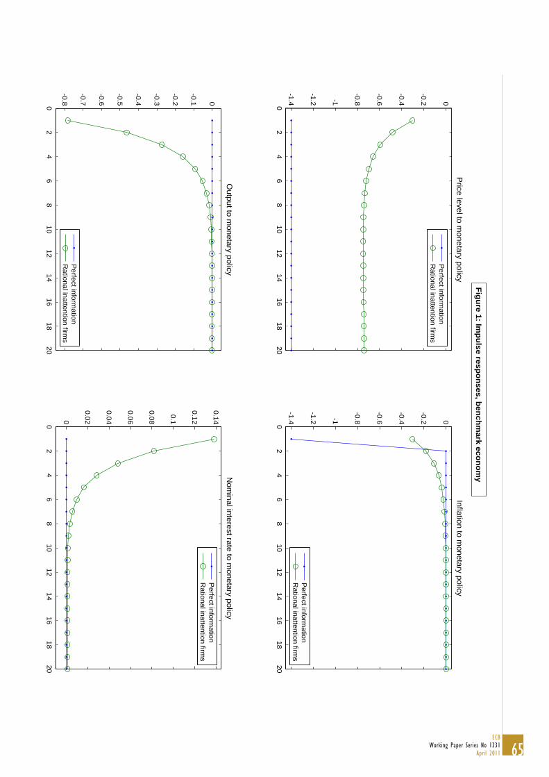
65ECB
Working Paper Series No 1331April 2011
02
46
810
1214
1618
20
-1.4
-1.2 -1
-0.8
-0.6
-0.4
-0.2 0
Price level to m
onetary policy
P
erfect information
Rational inattention firm
s
02
46
810
1214
1618
20
-1.4
-1.2 -1
-0.8
-0.6
-0.4
-0.2 0
Inflation to monetary policy
Perfect inform
ationR
ational inattention firms
02
46
810
1214
1618
20
-0.8
-0.7
-0.6
-0.5
-0.4
-0.3
-0.2
-0.1 0
Output to m
onetary policy
Perfect inform
ationR
ational inattention firms
02
46
810
1214
1618
20
0
0.02
0.04
0.06
0.08
0.1
0.12
0.14
Nom
inal interest rate to monetary policy
P
erfect information
Rational inattention firm
s
Figure 1: Impulse responses, benchm
ark economy

66ECBWorking Paper Series No 1331April 2011
02
46
810
1214
1618
20
-6 -5 -4 -3 -2 -1 0
Price level to aggregate technology
Perfect inform
ationR
ational inattention firms
02
46
810
1214
1618
20
-2.5 -2
-1.5 -1
-0.5 0
Inflation to aggregate technology
Perfect inform
ationR
ational inattention firms
02
46
810
1214
1618
20
0
0.1
0.2
0.3
0.4
0.5
0.6
0.7
0.8
0.9
Output to aggregate technology
Perfect inform
ationR
ational inattention firms
02
46
810
1214
1618
20-0.35
-0.3
-0.25
-0.2
-0.15
-0.1
-0.05 0
Nom
inal interest rate to aggregate technology
Perfect inform
ationR
ational inattention firms
Figure 2: Impulse responses, benchm
ark economy

67ECB
Working Paper Series No 1331April 2011
02
46
810
1214
1618
20
-9 -8 -7 -6 -5 -4 -3 -2 -1 0
Perfect inform
ationR
ational inattention firms
Figure 3: Impulse response of an individual price to a firm
-specific productivity shock, benchmark econom
y

68ECBWorking Paper Series No 1331April 2011
02
46
810
1214
1618
20
-1.4
-1.2 -1
-0.8
-0.6
-0.4
-0.2 0
Price level to m
onetary policy
Perfect inform
ationR
ational inattention firms
Calvo m
odel
02
46
810
1214
1618
20
-1.4
-1.2 -1
-0.8
-0.6
-0.4
-0.2 0
Inflation to monetary policy
Perfect inform
ationR
ational inattention firms
Calvo m
odel
02
46
810
1214
1618
20
-0.8
-0.7
-0.6
-0.5
-0.4
-0.3
-0.2
-0.1 0
Output to m
onetary policy
Perfect inform
ationR
ational inattention firms
Calvo m
odel
02
46
810
1214
1618
20
0
0.02
0.04
0.06
0.08
0.1
0.12
0.14
Nom
inal interest rate to monetary policy
Perfect inform
ationR
ational inattention firms
Calvo m
odel
Figure 4: Impulse responses, benchm
ark economy and Calvo m
odel

69ECB
Working Paper Series No 1331April 2011
02
46
810
1214
1618
20
-6 -5 -4 -3 -2 -1 0
Price level to aggregate technology
Perfect inform
ationR
ational inattention firms
Calvo m
odel
02
46
810
1214
1618
20
-2.5 -2
-1.5 -1
-0.5 0
Inflation to aggregate technology
Perfect inform
ationR
ational inattention firms
Calvo m
odel
02
46
810
1214
1618
20
-0.4
-0.2 0
0.2
0.4
0.6
0.8 1
Output to aggregate technology
Perfect inform
ationR
ational inattention firms
Calvo m
odel
02
46
810
1214
1618
20-0.35
-0.3
-0.25
-0.2
-0.15
-0.1
-0.05 0
Nom
inal interest rate to aggregate technology
Perfect inform
ationR
ational inattention firms
Calvo m
odel
Figure 5: Impulse responses, benchm
ark economy and Calvo m
odel

70ECBWorking Paper Series No 1331April 2011
1.051.25
1.51.75
23
510
0.95 1
1.05
1.1
1.15
1.2
1.25
1.3
Standard deviation of output gap due to m
onetary policy shocksPercent
φπ
1.051.25
1.51.75
23
510
0.4
0.45
0.5
0.55
0.6
0.65
0.7
0.75
0.8
0.85
0.9 Standard deviation of output gap due to aggregate technology shocks
Percent
φπ
1.051.25
1.51.75
23
510
0.3
0.4
0.5
0.6
0.7
0.8
0.9 1
1.1
1.2S
tandard deviation of output gap due to monetary policy shocks
Percent
φπ
1.051.25
1.51.75
23
510
0.5 1
1.5 2
2.5 3 Standard deviation of output gap due to aggregate technology shocks
Percent
φπ
Rational inattention firm
sR
ational inattention firms
Calvo m
odelC
alvo model
Figure 6: Standard deviation of output gap vs. parameter φπ , benchm
ark economy and Calvo m
odel
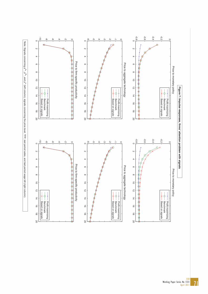
71ECB
Working Paper Series No 1331April 2011
02
46
810
1214
1618
20-0.8
-0.6
-0.4
-0.2 0P
rice to monetary policy
Profit-m
aximizing
Benchm
arkB
ased on signals
02
46
810
1214
1618
20-6 -5 -4 -3 -2 -1 0
Price to aggregate technology
Profit-m
aximizing
Benchm
arkB
ased on signals
02
46
810
1214
1618
20-10 -8 -6 -4 -2 0
Price to firm
-specific productivityProfit-m
aximizing
Benchm
arkB
ased on signals
02
46
810
1214
1618
20-0.8
-0.6
-0.4
-0.2 0P
rice to monetary policy
Profit-m
aximizing
Benchm
arkB
ased on signals
02
46
810
1214
1618
20-6 -5 -4 -3 -2 -1 0
Price to aggregate technology
Profit-m
aximizing
Benchm
arkB
ased on signals
02
46
810
1214
1618
20-10 -8 -6 -4 -2 0
Price to firm
-specific productivityProfit-m
aximizing
Benchm
arkB
ased on signals
Figure 7: Impulse responses, firm
s' attention problem with signals
Note: S
ignals concerning pA*, p
R*, and pI* (left colum
n), signals concerning the price level, TFP, last period sales, and last period w
age bill (right column).
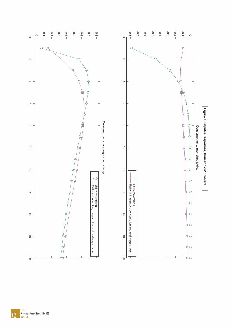
72ECBWorking Paper Series No 1331April 2011
02
46
810
1214
1618
20
-0.8
-0.7
-0.6
-0.5
-0.4
-0.3
-0.2
-0.1 0
Consum
ption to monetary policy
Utility-m
aximizing
Rational inattention, consum
ption and real wage chosen
02
46
810
1214
1618
20
0
0.1
0.2
0.3
0.4
0.5
0.6
0.7
0.8
Consum
ption to aggregate technology
Utility-m
aximizing
Rational inattention, consum
ption and real wage chosen
Figure 8: Impulse responses, households' problem
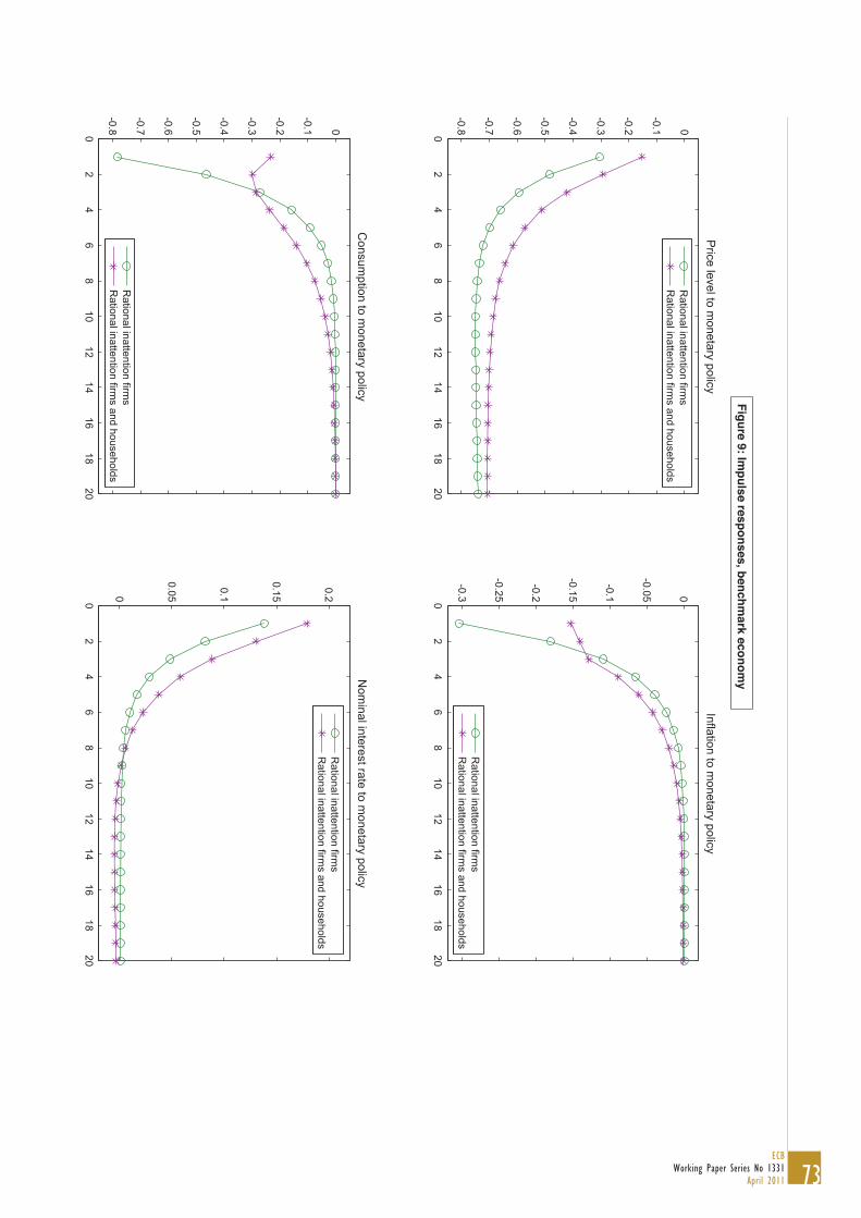
73ECB
Working Paper Series No 1331April 2011
02
46
810
1214
1618
20
-0.8
-0.7
-0.6
-0.5
-0.4
-0.3
-0.2
-0.1 0
Price level to m
onetary policy
Rational inattention firm
sR
ational inattention firms and households
02
46
810
1214
1618
20
-0.3
-0.25
-0.2
-0.15
-0.1
-0.05 0
Inflation to monetary policy
Rational inattention firm
sR
ational inattention firms and households
02
46
810
1214
1618
20
-0.8
-0.7
-0.6
-0.5
-0.4
-0.3
-0.2
-0.1 0
Consum
ption to monetary policy
Rational inattention firm
sR
ational inattention firms and households
02
46
810
1214
1618
20
0
0.05
0.1
0.15
0.2
Nom
inal interest rate to monetary policy
Rational inattention firm
sR
ational inattention firms and households
Figure 9: Impulse responses, benchm
ark economy
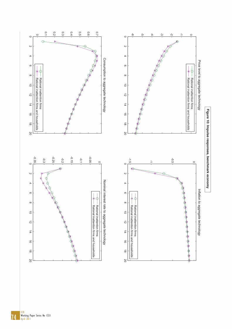
74ECBWorking Paper Series No 1331April 2011
02
46
810
1214
1618
20
-6 -5 -4 -3 -2 -1 0
Price level to aggregate technology
Rational inattention firm
sR
ational inattention firms and households
02
46
810
1214
1618
20-1.5 -1
-0.5 0
Inflation to aggregate technology
Rational inattention firm
sR
ational inattention firms and households
02
46
810
1214
1618
20
0
0.1
0.2
0.3
0.4
0.5
0.6
0.7
Consum
ption to aggregate technology
Rational inattention firm
sR
ational inattention firms and households
02
46
810
1214
1618
20-0.35
-0.3
-0.25
-0.2
-0.15
-0.1
-0.05 0
Nom
inal interest rate to aggregate technology
Rational inattention firm
sR
ational inattention firms and households
Figure 10: Impulse responses, benchm
ark economy

WORK ING PAPER SER I E SNO 1313 / MARCH 2011
by Cristian Badarinzaand Emil Margaritov
NEWS AND POLICY FORESIGHT IN A MACRO-FINANCE MODEL OF THE US