business intelligence - cdn.ttgtmedia.com · warehousing, olap, and data mining as business...

147

8Business Intelligence

Business intelligence has become a buzzword in recent years. The data-base tools found under the heading of business intelligence include datawarehousing, online analytical processing (OLAP), and data mining. Thefunctionalities of these tools are complementary and interrelated. Datawarehousing provides for the efficient storage, maintenance, and retrievalof historical data. OLAP is a service that provides quick answers to ad hocqueries against the data warehouse. Data mining algorithms find patternsin the data and report models back to the user. All three tools are relatedto the way data in a data warehouse are logically organized, and perfor-mance is highly sensitive to the database design techniques used [Bar-quin and Edelstein, 1997]. The encompassing goal for business intelli-gence technologies is to provide useful information for decision support.

Each of the major DBMS vendors is marketing the tools for datawarehousing, OLAP, and data mining as business intelligence. This chap-ter covers each of these technologies in turn. We take a close look at therequirements for a data warehouse; its basic components and principlesof operation; the critical issues in its design; and the important logicaldatabase design elements in its environment. We then investigate thebasic elements of OLAP and data mining as special query techniquesapplied to data warehousing. We cover data warehousing in Section 8.1,OLAP in Section 8.2, and data mining in Section 8.3.

148 CHAPTER 8 Business Intelligence

8.1 Data Warehousing

A data warehouse is a large repository of historical data that can be inte-grated for decision support. The use of a data warehouse is markedly dif-ferent from the use of operational systems. Operational systems containthe data required for the day-to-day operations of an organization. Thisoperational data tends to change quickly and constantly. The table sizesin operational systems are kept manageably small by periodically purg-ing old data. The data warehouse, by contrast, periodically receives his-torical data in batches, and grows over time. The vast size of data ware-houses can run to hundreds of gigabytes, or even terabytes. The problemthat drives data warehouse design is the need for quick results to queriesposed against huge amounts of data. The contrasting aspects of datawarehouses and operational systems result in a distinctive designapproach for data warehousing.

8.1.1 Overview of Data Warehousing

A data warehouse contains a collection of tools for decision supportassociated with very large historical databases, which enables the enduser to make quick and sound decisions. Data warehousing grew out ofthe technology for decision support systems (DSS) and executive infor-mation systems (EIS). DSSs are used to analyze data from commonlyavailable databases with multiple sources, and to create reports. Thereport data is not time critical in the sense that a real-time system is, butit must be timely for decision making. EISs are like DSSs, but more pow-erful, easier to use, and more business specific. EISs were designed to pro-vide an alternative to the classical online transaction processing (OLTP)systems common to most commercially available database systems.OLTP systems are often used to create common applications, includingthose with mission-critical deadlines or response times. Table 8.1 sum-marizes the basic differences between OLTP and data warehouse systems.

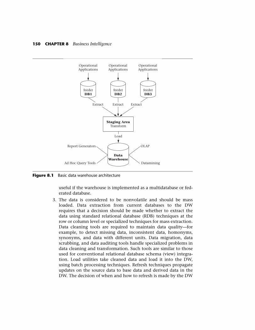
The basic architecture for a data warehouse environment is shown inFigure 8.1. The diagram shows that the data warehouse is stocked by avariety of source databases from possibly different geographical loca-tions. Each source database serves its own applications, and the datawarehouse serves a DSS/EIS with its informational requests. Each feedersystem database must be reconciled with the data warehouse datamodel; this is accomplished during the process of extracting therequired data from the feeder database system, transforming the data

8.1 Data Warehousing 149

from the feeder system to the data warehouse, and loading the data intothe data warehouse [Cataldo, 1997].

Core Requirements for Data Warehousing

Let us now take a look at the core requirements and principles that guidethe design of data warehouses (DWs) [Simon, 1995; Barquin and Edel-stein, 1997; Chaudhuri and Dayal, 1997; Gray and Watson, 1998]:

1. DWs are organized around subject areas. Subject areas are analo-gous to the concept of functional areas, such as sales, projectmanagement, or employees, as discussed in the context of ER dia-gram clustering in Section 4.5. Each subject area has its own con-ceptual schema and can be represented using one or more entitiesin the ER data model or by one or more object classes in theobject-oriented data model. Subject areas are typically indepen-dent of individual transactions involving data creation or manip-ulation. Metadata repositories are needed to describe sourcedatabases, DW objects, and ways of transforming data from thesources to the DW.

2. DWs should have some integration capability. A common datarepresentation should be designed so that all the different indi-vidual representations can be mapped to it. This is particularly

Table 8.1 Comparison between OLTP and Data Warehouse Databases

OLTP Data Warehouse

Transaction oriented Business process oriented

Thousands of users Few users (typically under 100)

Generally small (MB up to several GB) Large (from hundreds of GB to several TB)

Current data Historical data

Normalized data(many tables, few columns per table)

Denormalized data(few tables, many columns per table)

Continuous updates Batch updates*

Simple to complex queries Usually very complex queries

* There is currently a push in the industry towards “active warehousing,” in which thewarehouse receives data in continuous updates. See Section 8.2.5 for further discussion.


useful if the warehouse is implemented as a multidatabase or fed-erated database.

3. The data is considered to be nonvolatile and should be massloaded. Data extraction from current databases to the DWrequires that a decision should be made whether to extract thedata using standard relational database (RDB) techniques at therow or column level or specialized techniques for mass extraction.Data cleaning tools are required to maintain data quality—forexample, to detect missing data, inconsistent data, homonyms,synonyms, and data with different units. Data migration, datascrubbing, and data auditing tools handle specialized problems indata cleaning and transformation. Such tools are similar to thoseused for conventional relational database schema (view) integra-tion. Load utilities take cleaned data and load it into the DW,using batch processing techniques. Refresh techniques propagateupdates on the source data to base data and derived data in theDW. The decision of when and how to refresh is made by the DW

Figure 8.1 Basic data warehouse architecture

feederDB1

OperationalApplications



feederDB2

feederDB3

DataWarehouse

Extract

Report Generators

Ad Hoc Query Tools

OLAP

Datamining

Extract Extract

Staging AreaTransform

Load


administrator and depends on user needs (e.g., OLAP needs) andexisting traffic to the DW.

4. Data tends to exist at multiple levels of granularity. Most impor-tant, the data tends to be of a historical nature, with potentiallyhigh time variance. In general, however, granularity can varyaccording to many different dimensions, not only by time framebut also by geographic region, type of product manufactured orsold, type of store, and so on. The sheer size of the databases is amajor problem in the design and implementation of DWs, espe-cially for certain queries, updates, and sequential backups. Thisnecessitates a critical decision between using a relational database(RDB) or a multidimensional database (MDD) for the implemen-tation of a DW.

5. The DW should be flexible enough to meet changing require-ments rapidly. Data definitions (schemas) must be broad enoughto anticipate the addition of new types of data. For rapidly chang-ing data retrieval requirements, the types of data and levels ofgranularity actually implemented must be chosen carefully.

6. The DW should have a capability for rewriting history, that is,allowing for “what-if” analysis. The DW should allow the admin-istrator to update historical data temporarily for the purpose of“what-if” analysis. Once the analysis is completed, the data mustbe correctly rolled back. This condition assumes that the data areat the proper level of granularity in the first place.

7. A usable DW user interface should be selected. The leadingchoices today are SQL, multidimensional views of relational data,or a special-purpose user interface. The user interface languagemust have tools for retrieving, formatting, and analyzing data.

8. Data should be either centralized or distributed physically. TheDW should have the capability to handle distributed data over anetwork. This requirement will become more critical as the use ofDWs grows and the sources of data expand.

The Life Cycle of Data Warehouses

Entire books have been written about select portions of the data ware-house life cycle. Our purpose in this section is to present some of thebasics and give the flavor of data warehousing. We strongly encouragethose who wish to pursue data warehousing to continue learningthrough other books dedicated to data warehousing. Kimball and Ross


[1998, 2002] have a series of excellent books covering the details of datawarehousing activities.

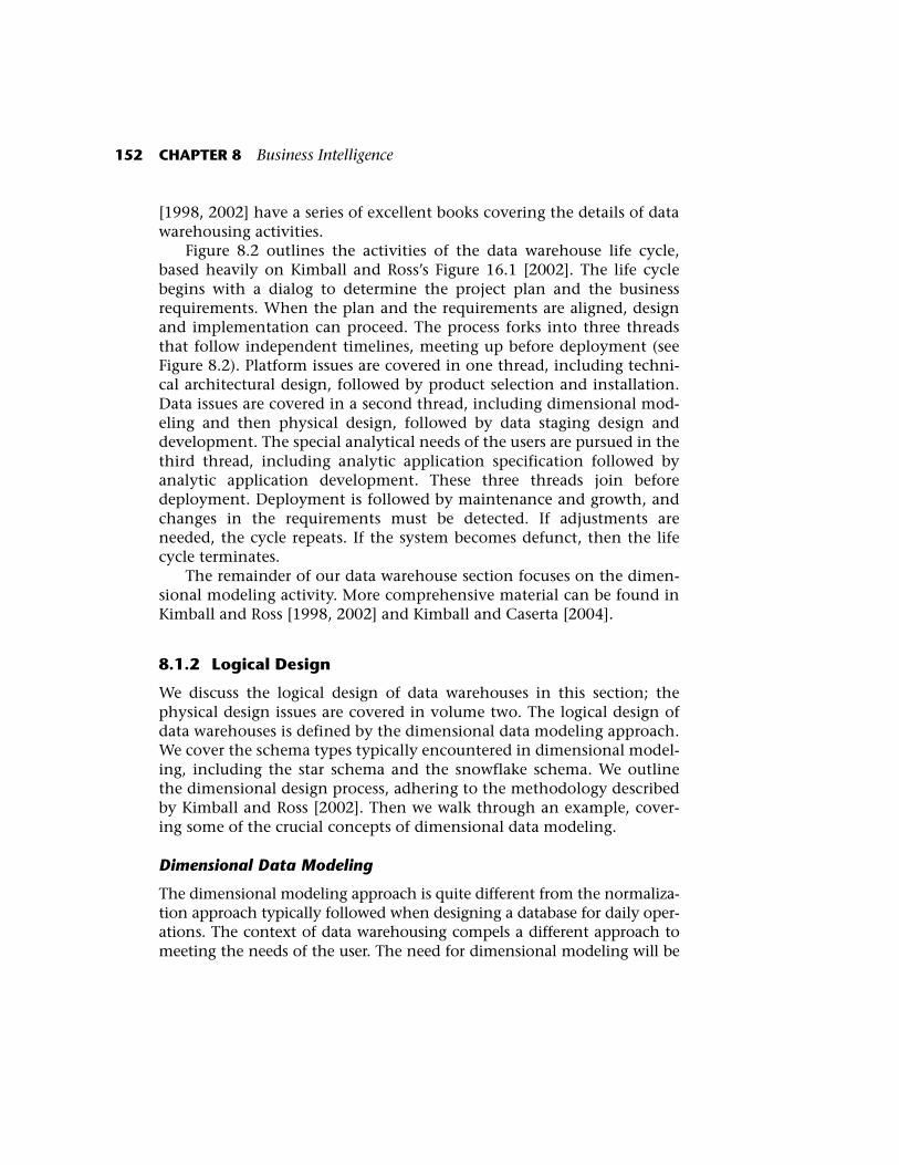
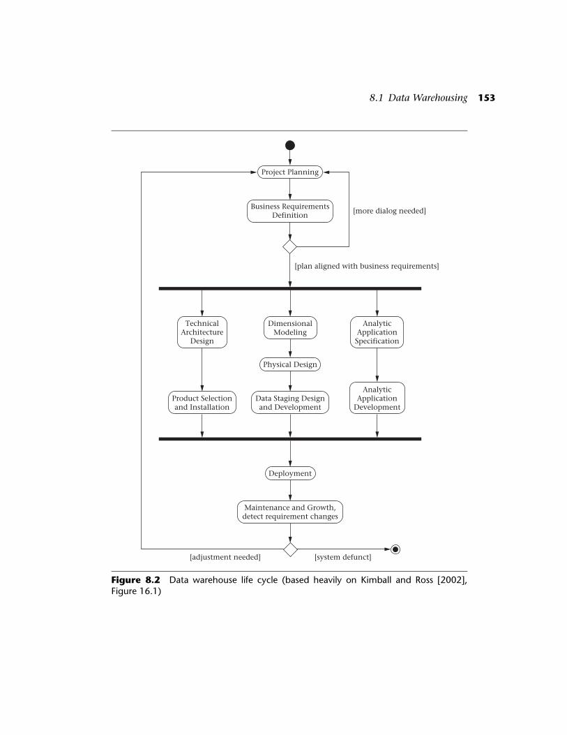
Figure 8.2 outlines the activities of the data warehouse life cycle,based heavily on Kimball and Ross’s Figure 16.1 [2002]. The life cyclebegins with a dialog to determine the project plan and the businessrequirements. When the plan and the requirements are aligned, designand implementation can proceed. The process forks into three threadsthat follow independent timelines, meeting up before deployment (seeFigure 8.2). Platform issues are covered in one thread, including techni-cal architectural design, followed by product selection and installation.Data issues are covered in a second thread, including dimensional mod-eling and then physical design, followed by data staging design anddevelopment. The special analytical needs of the users are pursued in thethird thread, including analytic application specification followed byanalytic application development. These three threads join beforedeployment. Deployment is followed by maintenance and growth, andchanges in the requirements must be detected. If adjustments areneeded, the cycle repeats. If the system becomes defunct, then the lifecycle terminates.

The remainder of our data warehouse section focuses on the dimen-sional modeling activity. More comprehensive material can be found inKimball and Ross [1998, 2002] and Kimball and Caserta [2004].

8.1.2 Logical Design

We discuss the logical design of data warehouses in this section; thephysical design issues are covered in volume two. The logical design ofdata warehouses is defined by the dimensional data modeling approach.We cover the schema types typically encountered in dimensional model-ing, including the star schema and the snowflake schema. We outlinethe dimensional design process, adhering to the methodology describedby Kimball and Ross [2002]. Then we walk through an example, cover-ing some of the crucial concepts of dimensional data modeling.

Dimensional Data Modeling

The dimensional modeling approach is quite different from the normaliza-tion approach typically followed when designing a database for daily oper-ations. The context of data warehousing compels a different approach tomeeting the needs of the user. The need for dimensional modeling will be


Figure 8.2 Data warehouse life cycle (based heavily on Kimball and Ross [2002],Figure 16.1)

Project Planning

Business RequirementsDefinition

DimensionalModeling

Physical Design

Data Staging Designand Development

Deployment

Maintenance and Growth,detect requirement changes

TechnicalArchitecture

Design

Product Selectionand Installation

AnalyticApplicationSpecification

AnalyticApplication

Development

[plan aligned with business requirements]

[more dialog needed]

[adjustment needed] [system defunct]


discussed further as we proceed. If you haven’t been exposed to data ware-housing before, be prepared for some new paradigms.

The Star Schema

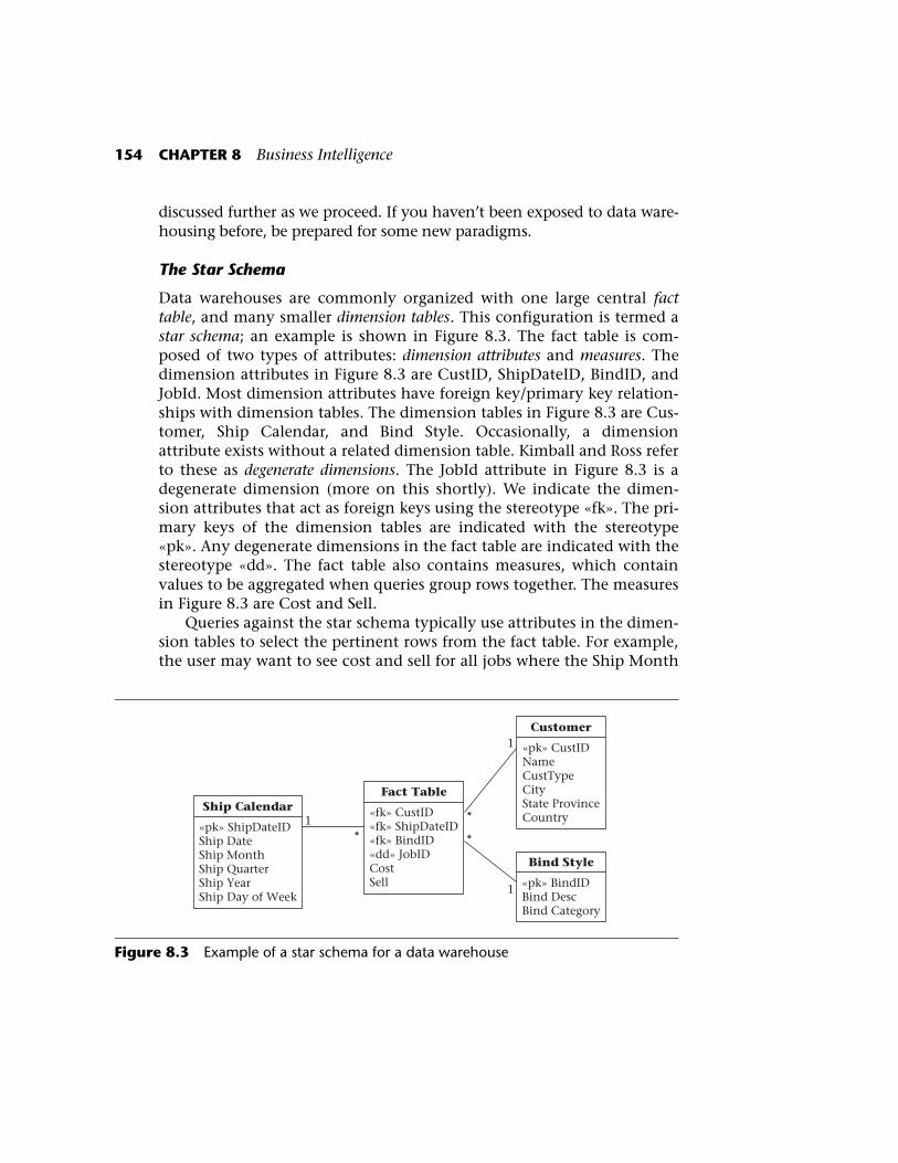
Data warehouses are commonly organized with one large central facttable, and many smaller dimension tables. This configuration is termed astar schema; an example is shown in Figure 8.3. The fact table is com-posed of two types of attributes: dimension attributes and measures. Thedimension attributes in Figure 8.3 are CustID, ShipDateID, BindID, andJobId. Most dimension attributes have foreign key/primary key relation-ships with dimension tables. The dimension tables in Figure 8.3 are Cus-tomer, Ship Calendar, and Bind Style. Occasionally, a dimensionattribute exists without a related dimension table. Kimball and Ross referto these as degenerate dimensions. The JobId attribute in Figure 8.3 is adegenerate dimension (more on this shortly). We indicate the dimen-sion attributes that act as foreign keys using the stereotype «fk». The pri-mary keys of the dimension tables are indicated with the stereotype«pk». Any degenerate dimensions in the fact table are indicated with thestereotype «dd». The fact table also contains measures, which containvalues to be aggregated when queries group rows together. The measuresin Figure 8.3 are Cost and Sell.

Queries against the star schema typically use attributes in the dimen-sion tables to select the pertinent rows from the fact table. For example,the user may want to see cost and sell for all jobs where the Ship Month

Figure 8.3 Example of a star schema for a data warehouse

Ship Calendar

«pk» ShipDateIDShip DateShip MonthShip QuarterShip YearShip Day of Week

Fact Table

«fk» CustID«fk» ShipDateID«fk» BindID«dd» JobIDCostSell

Customer

«pk» CustIDNameCustTypeCityState ProvinceCountry

Bind Style

«pk» BindIDBind DescBind Category

*

*

1

1

1*


is January 2005. The dimension table attributes are also typically used togroup the rows in useful ways when exploring summary information.For example, the user may wish to see the total cost and sell for eachShip Month in the Ship Year 2005. Notice that dimension tables canallow different levels of detail the user can examine. For example, theFigure 8.3 schema allows the fact table rows to be grouped by Ship Date,Month, Quarter or Year. These dimension levels form a hierachy. There isalso a second hierarchy in the Ship Calendar dimension that allows theuser to group fact table rows by the day of the week. The user can moveup or down a hierarchy when exploring the data. Moving down a hierar-chy to examine more detailed data is a drill-down operation. Moving up ahierarchy to summarize details is a roll-up operation.

Together, the dimension attributes compose a candidate key of thefact table. The level of detail defined by the dimension attributes is thegranularity of the fact table. When designing a fact table, the granularityshould be the most detailed level available that any user would wish toexamine. This requirement sometimes means that a degenerate dimen-sion, such as JobId in Figure 8.3, must be included. The JobId in this starschema is not used to select or group rows, so there is no related dimen-sion table. The purpose of the JobId attribute is to distinguish rows atthe correct level of granularity. Without the JobId attribute, the facttable would group together similar jobs, prohibiting the user from exam-ining the cost and sell values of individual jobs.

Normalization is not the guiding principle in data warehouse design.The purpose of data warehousing is to provide quick answers to queriesagainst a large set of historical data. Star schema organization facilitatesquick response to queries in the context of the data warehouse. The coredetailed data are centralized in the fact table. Dimensional informationand hierarchies are kept in dimension tables, a single join away from thefact table. The hierarchical levels of data contained in the dimensiontables of Figure 8.3 violate 3NF, but these violations to the principles ofnormalization are justified. The normalization process would break eachdimension table in Figure 8.3 into multiple tables. The resulting normal-ized schema would require more join processing for most queries. Thedimension tables are small in comparison to the fact table, and typicallyslow changing. The bulk of operations in the data warehouse are readoperations. The benefits of normalization are low when most operationsare read only. The benefits of minimizing join operations overwhelm thebenefits of normalization in the context of data warehousing. Themarked differences between the data warehouse environment and the


operational system environment lead to distinct design approaches.Dimensional modeling is the guiding principle in data warehousedesign.

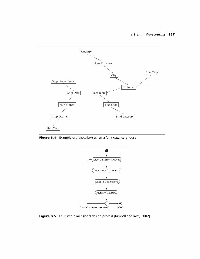
Snowflake Schema

The data warehouse literature often refers to a variation of the starschema known as the snowflake schema. Normalizing the dimensiontables in a star schema leads to a snowflake schema. Figure 8.4 shows thesnowflake schema analogous to the star schema of Figure 8.3. Noticethat each hierarchical level becomes its own table. The snowflakeschema is generally losing favor. Kimball and Ross strongly prefer thestar schema, due to its speed and simplicity. Not only does the starschema yield quicker query response, it is also easier for the user tounderstand when building queries. We include the snowflake schemahere for completeness.

Dimensional Design Process

We adhere to the four-step dimensional design process promoted by Kim-ball and Ross. Figure 8.5 outlines the activities in the four-step process.

Dimensional Modeling Example

Congratulations, you are now the owner of the ACME Data Mart Com-pany! Your company builds data warehouses. You consult with othercompanies, design and deploy data warehouses to meet their needs, andsupport them in their efforts.

Your first customer is XYZ Widget, Inc. XYZ Widget is a manufactur-ing company with information systems in place. These are operationalsystems that track the current and recent state of the various businessprocesses. Older records that are no longer needed for operating theplant are purged. This keeps the operational systems running efficiently.

XYZ Widget is now ten years old, and growing fast. The managementrealizes that information is valuable. The CIO has been saving databefore they are purged from the operational system. There are tens ofmillions of historical records, but there is no easy way to access the datain a meaningful way. ACME Data Mart has been called in to design andbuild a DSS to access the historical data.

Discussions with XYZ Widget commence. There are many questionsthey want to have answered by analyzing the historical data. You beginby making a list of what XYZ wants to know.


Figure 8.4 Example of a snowflake schema for a data warehouse

Figure 8.5 Four step dimensional design process [Kimball and Ross, 2002]

Fact TableShip Date

Bind Style

Customer

Ship Day of Week

Ship Month

Ship Quarter

Ship Year

Bind Category

City

State Province

Country

Cust Type

Select a Business Process

Choose Dimensions

Identify Measures

Determine Granularity

[more business processes] [else]


XYZ Widget Company Wish List

1. What are the trends of our various products in terms of sales dol-lars, unit volume, and profit margin?

2. For those products that are not profitable, can we drill down anddetermine why they are not profitable?

3. How accurately do our estimated costs match our actual costs?

4. When we change our estimating calculations, how are sales andprofitability affected?

5. What are the trends in the percentage of jobs that ship on time?

6. What are the trends in productivity by department, for eachmachine, and for each employee?

7. What are the trends in meeting the scheduled dates for eachdepartment, and for each machine?

8. How effective was the upgrade on machine 123?

9. Which customers bring the most profitable jobs?

10. How do our promotional bulk discounts affect sales and profit-ability?

Looking over the wish list, you begin picking out the business pro-cesses involved. The following list is sufficient to satisfy the items on thewish list.

Business Processes

1. Estimating

2. Scheduling

3. Productivity Tracking

4. Job Costing

These four business processes are interlinked in the XYZ Widget Com-pany. Let’s briefly walk through the business processes and the organiza-tion of information in the operational systems, so we have an idea whatinformation is available for analysis. For each business process, we’lldesign a star schema for storing the data.

The estimating process begins by entering widget specifications. Thetype of widget determines which machines are used to manufacture thewidget. The estimating software then calculates estimated time on each


machine used to produce that particular type of widget. Each machine ismodeled with a standard setup time and running speed. If a particulartype of widget is difficult to process on a particular machine, the timesare adjusted accordingly. Each machine has an hourly rate. The esti-mated time is multiplied by the rate to give labor cost. Each estimatestores widget specifications, a breakdown of the manufacturing costs,the markup and discount applied (if any), and the price. The quote issent to the customer. If the customer accepts the quote, then the quoteis associated with a job number, the specifications are printed as a jobticket, and the job ticket moves to scheduling.

We need to determine the grain before designing a schema for theestimating data mart. The grain should be at the most detailed level, giv-ing the greatest flexibility for drill-down operations when users areexploring the data. The most granular level in the estimating process isthe estimating detail. Each estimating detail record specifies informationfor an individual cost center for a given estimate. This is the finest gran-ularity of estimating data in the operational system, and this level ofdetail is also potentially valuable for the data warehouse users.

The next design step is to determine the dimensions. Looking at theestimating detail, we see that the associated attributes are the job specifi-cations, the estimate number and date, the job number and win date ifthe estimate becomes a job, the customer, the promotion, the cost cen-ter, the widget quantity, estimated hours, hourly rate, estimated cost,markup, discount, and price. Dimensions are those attributes that theusers want to group by when exploring the data. The users are interestedin grouping by the various job specifications and by the cost center. Theusers also need to be able to group by date ranges. The estimate date andthe win date are both of interest. Grouping by customer and promotionare also of interest to the users. These become the dimensions of the starschema for the estimating process.

Next, we identify the measures. Measures are the columns that con-tain values to be aggregated when rows are grouped together. The mea-sures in the estimating process are estimated hours, hourly rate, esti-mated cost, markup, discount, and price.

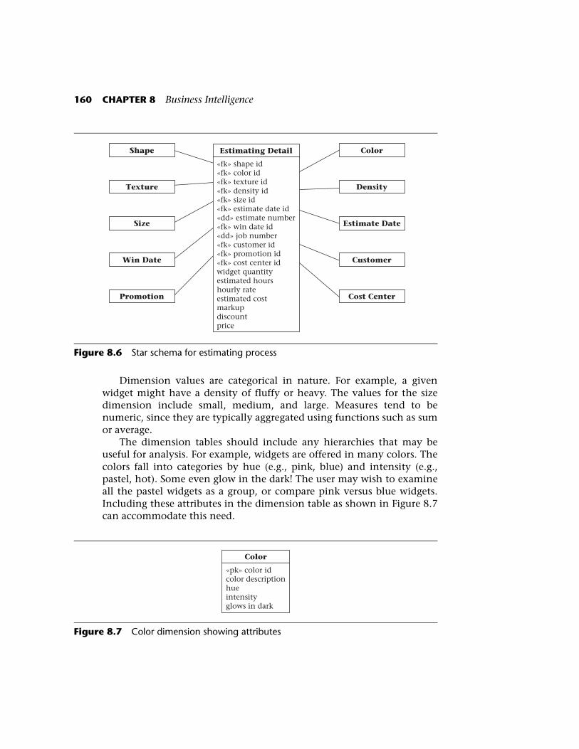
The star schema resulting from the analysis of the estimating processis shown in Figure 8.6. There are five widget qualities of interest: shape,color, texture, density, and size. For example, a given widget might be amedium round red fuzzy fluffy widget. The estimate and job numbersare included as degenerate dimensions. The rest of the dimensions andmeasures are as outlined in the previous two paragraphs.


Dimension values are categorical in nature. For example, a givenwidget might have a density of fluffy or heavy. The values for the sizedimension include small, medium, and large. Measures tend to benumeric, since they are typically aggregated using functions such as sumor average.

The dimension tables should include any hierarchies that may beuseful for analysis. For example, widgets are offered in many colors. Thecolors fall into categories by hue (e.g., pink, blue) and intensity (e.g.,pastel, hot). Some even glow in the dark! The user may wish to examineall the pastel widgets as a group, or compare pink versus blue widgets.Including these attributes in the dimension table as shown in Figure 8.7can accommodate this need.

Figure 8.6 Star schema for estimating process

Figure 8.7 Color dimension showing attributes

«fk» shape id«fk» color id«fk» texture id«fk» density id«fk» size id«fk» estimate date id«dd» estimate number«fk» win date id«dd» job number«fk» customer id«fk» promotion id«fk» cost center idwidget quantityestimated hourshourly rateestimated costmarkupdiscountprice

Estimating DetailShape Color

Texture Density

Size Estimate Date

Customer

Promotion Cost Center

Win Date

Color

«pk» color idcolor descriptionhueintensityglows in dark


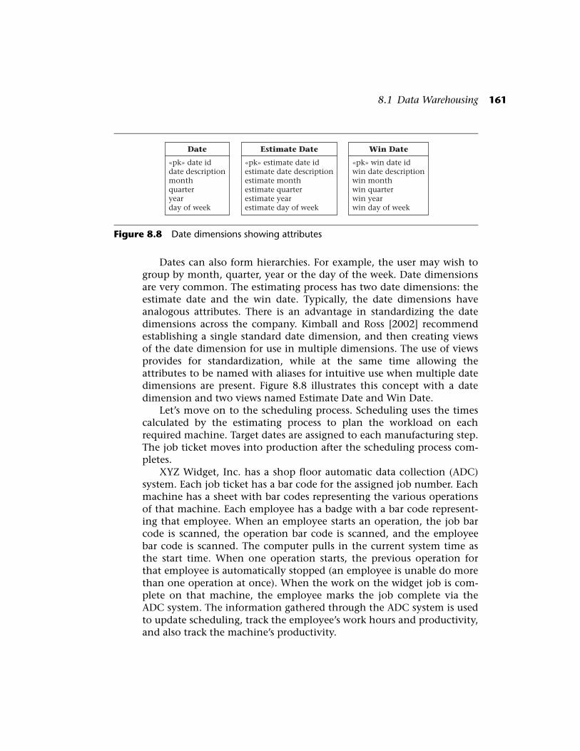
Dates can also form hierarchies. For example, the user may wish togroup by month, quarter, year or the day of the week. Date dimensionsare very common. The estimating process has two date dimensions: theestimate date and the win date. Typically, the date dimensions haveanalogous attributes. There is an advantage in standardizing the datedimensions across the company. Kimball and Ross [2002] recommendestablishing a single standard date dimension, and then creating viewsof the date dimension for use in multiple dimensions. The use of viewsprovides for standardization, while at the same time allowing theattributes to be named with aliases for intuitive use when multiple datedimensions are present. Figure 8.8 illustrates this concept with a datedimension and two views named Estimate Date and Win Date.

Let’s move on to the scheduling process. Scheduling uses the timescalculated by the estimating process to plan the workload on eachrequired machine. Target dates are assigned to each manufacturing step.The job ticket moves into production after the scheduling process com-pletes.

XYZ Widget, Inc. has a shop floor automatic data collection (ADC)system. Each job ticket has a bar code for the assigned job number. Eachmachine has a sheet with bar codes representing the various operationsof that machine. Each employee has a badge with a bar code represent-ing that employee. When an employee starts an operation, the job barcode is scanned, the operation bar code is scanned, and the employeebar code is scanned. The computer pulls in the current system time asthe start time. When one operation starts, the previous operation forthat employee is automatically stopped (an employee is unable do morethan one operation at once). When the work on the widget job is com-plete on that machine, the employee marks the job complete via theADC system. The information gathered through the ADC system is usedto update scheduling, track the employee’s work hours and productivity,and also track the machine’s productivity.

Figure 8.8 Date dimensions showing attributes

Date

«pk» date iddate descriptionmonthquarteryearday of week

Win Date

«pk» win date idwin date descriptionwin monthwin quarterwin yearwin day of week

Estimate Date

«pk» estimate date idestimate date descriptionestimate monthestimate quarterestimate yearestimate day of week


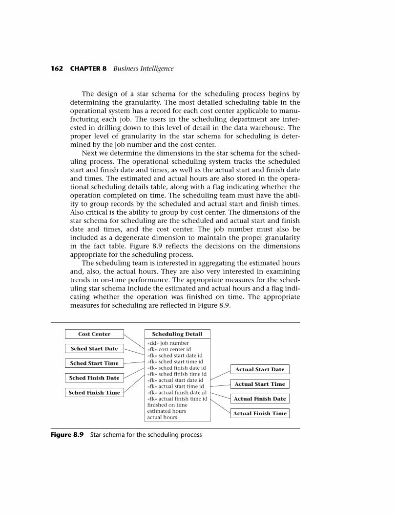
The design of a star schema for the scheduling process begins bydetermining the granularity. The most detailed scheduling table in theoperational system has a record for each cost center applicable to manu-facturing each job. The users in the scheduling department are inter-ested in drilling down to this level of detail in the data warehouse. Theproper level of granularity in the star schema for scheduling is deter-mined by the job number and the cost center.

Next we determine the dimensions in the star schema for the sched-uling process. The operational scheduling system tracks the scheduledstart and finish date and times, as well as the actual start and finish dateand times. The estimated and actual hours are also stored in the opera-tional scheduling details table, along with a flag indicating whether theoperation completed on time. The scheduling team must have the abil-ity to group records by the scheduled and actual start and finish times.Also critical is the ability to group by cost center. The dimensions of thestar schema for scheduling are the scheduled and actual start and finishdate and times, and the cost center. The job number must also beincluded as a degenerate dimension to maintain the proper granularityin the fact table. Figure 8.9 reflects the decisions on the dimensionsappropriate for the scheduling process.

The scheduling team is interested in aggregating the estimated hoursand, also, the actual hours. They are also very interested in examiningtrends in on-time performance. The appropriate measures for the sched-uling star schema include the estimated and actual hours and a flag indi-cating whether the operation was finished on time. The appropriatemeasures for scheduling are reflected in Figure 8.9.

Figure 8.9 Star schema for the scheduling process

«dd» job number«fk» cost center id«fk» sched start date id«fk» sched start time id«fk» sched finish date id«fk» sched finish time id«fk» actual start date id«fk» actual start time id«fk» actual finish date id«fk» actual finish time idfinished on timeestimated hoursactual hours

Scheduling DetailCost Center

Sched Start Date

Actual Start DateSched Start Time

Actual Start Time

Actual Finish DateSched Finish Time

Actual Finish Time

Sched Finish Date


There are several standardization principles in play in Figure 8.9.Note that there are multiple time dimensions. These should be standard-ized with a single time dimension, along with views filling the differentroles, similar to the approach used for the date dimensions. Also, noticethe Cost Center dimension is present both in the estimating and thescheduling processes. These are actually the same, and should bedesigned as a single dimension. Dimensions can be shared between mul-tiple star schemas. One last point: the estimated hours are carried fromestimating into scheduling in the operational systems. These numbersfeed into the star schemas for both the estimating and the schedulingprocesses. The meaning is the same between the two attributes; there-fore, they are both named “estimated hours.” The rule of thumb is thatif two attributes carry the same meaning, they should be named thesame, and if two attributes are named the same, they carry the samemeaning. This consistency allows discussion and comparison of infor-mation between business processes across the company.

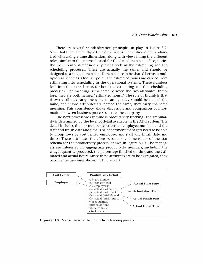
The next process we examine is productivity tracking. The granular-ity is determined by the level of detail available in the ADC system. Thedetail includes the job number, cost center, employee number, and thestart and finish date and time. The department managers need to be ableto group rows by cost center, employee, and start and finish date andtimes. These attributes therefore become the dimensions of the starschema for the productivity process, shown in Figure 8.10. The manag-ers are interested in aggregating productivity numbers, including thewidget quantity produced, the percentage finished on time and the esti-mated and actual hours. Since these attributes are to be aggregated, theybecome the measures shown in Figure 8.10.

Figure 8.10 Star schema for the productivity tracking process

«dd» job number«fk» cost center id«fk» employee id«fk» actual start date id«fk» actual start time id«fk» actual finish date id«fk» actual finish time idwidget quantityfinished on timeestimated hoursactual hours

Productivity DetailCost Center

Employee Actual Start Date

Actual Start Time

Actual Finish Date

Actual Finish Time


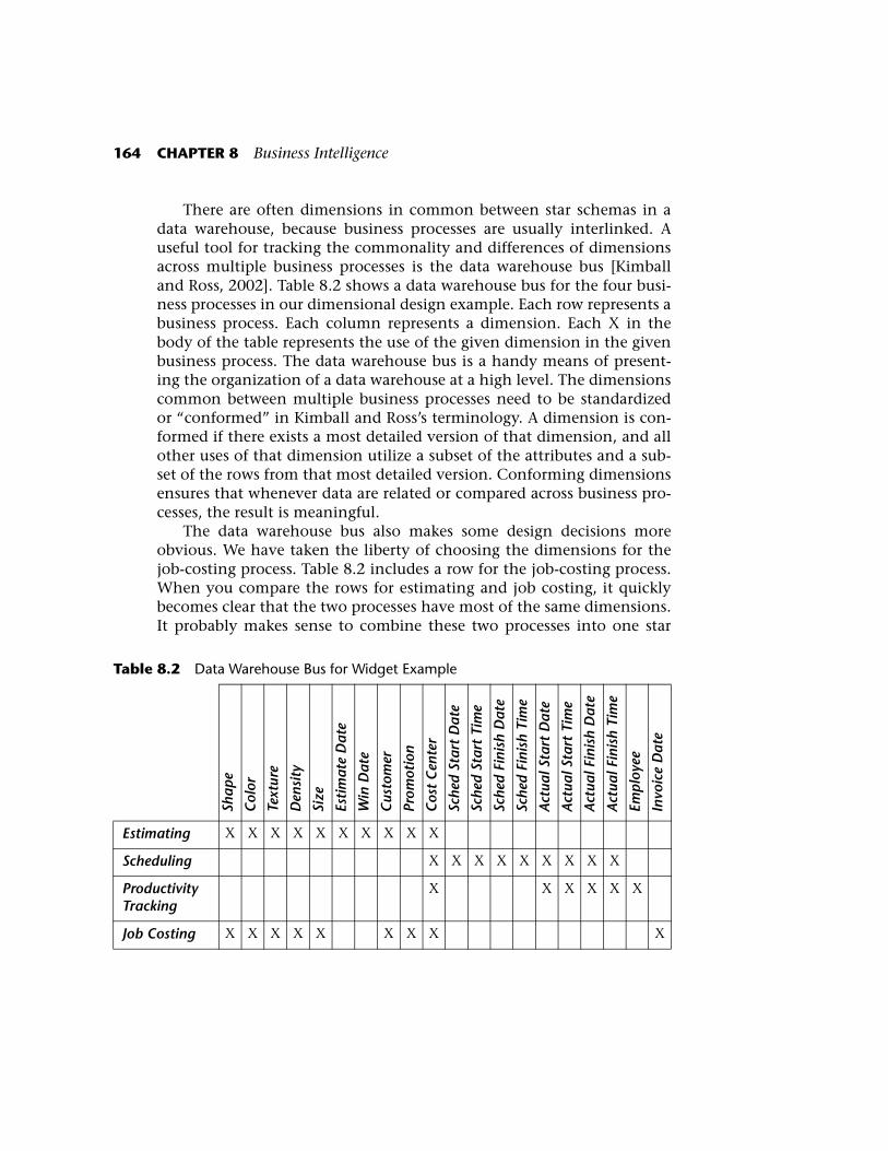
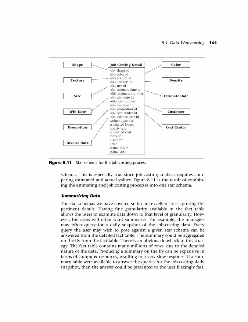
There are often dimensions in common between star schemas in adata warehouse, because business processes are usually interlinked. Auseful tool for tracking the commonality and differences of dimensionsacross multiple business processes is the data warehouse bus [Kimballand Ross, 2002]. Table 8.2 shows a data warehouse bus for the four busi-ness processes in our dimensional design example. Each row represents abusiness process. Each column represents a dimension. Each X in thebody of the table represents the use of the given dimension in the givenbusiness process. The data warehouse bus is a handy means of present-ing the organization of a data warehouse at a high level. The dimensionscommon between multiple business processes need to be standardizedor “conformed” in Kimball and Ross’s terminology. A dimension is con-formed if there exists a most detailed version of that dimension, and allother uses of that dimension utilize a subset of the attributes and a sub-set of the rows from that most detailed version. Conforming dimensionsensures that whenever data are related or compared across business pro-cesses, the result is meaningful.

The data warehouse bus also makes some design decisions moreobvious. We have taken the liberty of choosing the dimensions for thejob-costing process. Table 8.2 includes a row for the job-costing process.When you compare the rows for estimating and job costing, it quicklybecomes clear that the two processes have most of the same dimensions.It probably makes sense to combine these two processes into one star

Table 8.2 Data Warehouse Bus for Widget Example

Shap

e

Col

or

Text

ure

Den

sity

Size

Esti

mat

e D

ate

Win

Dat

e

Cus

tom

er

Prom

otio

n

Cos

t C

ente

r

Sche

d St

art

Dat

e

Sche

d St

art

Tim

e

Sche

d Fi

nish

Dat

e

Sche

d Fi

nish

Tim

e

Act

ual S

tart

Dat

e

Act

ual S

tart

Tim

e

Act

ual F

inis

h D

ate

Act

ual F

inis

h Ti

me

Empl

oyee

Invo

ice

Dat

e

Estimating X X X X X X X X X X

Scheduling X X X X X X X X X

Productivity Tracking

X X X X X X

Job Costing X X X X X X X X X


schema. This is especially true since job-costing analysis requires com-paring estimated and actual values. Figure 8.11 is the result of combin-ing the estimating and job costing processes into one star schema.

Summarizing Data

The star schemas we have covered so far are excellent for capturing thepertinent details. Having fine granularity available in the fact tableallows the users to examine data down to that level of granularity. How-ever, the users will often want summaries. For example, the managersmay often query for a daily snapshot of the job-costing data. Everyquery the user may wish to pose against a given star schema can beanswered from the detailed fact table. The summary could be aggregatedon the fly from the fact table. There is an obvious drawback to this strat-egy. The fact table contains many millions of rows, due to the detailednature of the data. Producing a summary on the fly can be expensive interms of computer resources, resulting in a very slow response. If a sum-mary table were available to answer the queries for the job costing dailysnapshot, then the answer could be presented to the user blazingly fast.

Figure 8.11 Star schema for the job costing process

«fk» shape id«fk» color id«fk» texture id«fk» density id«fk» size id«fk» estimate date id«dd» estimate number«fk» win date id«dd» job number«fk» customer id«fk» promotion id«fk» cost center id«fk» invoice date idwidget quantityestimated hourshourly rateestimated costmarkupdiscountpriceactual hoursactual cost

Job Costing DetailShape Color

Texture Density

Size Estimate Date

Customer

Promotion Cost Center

Win Date

Invoice Date


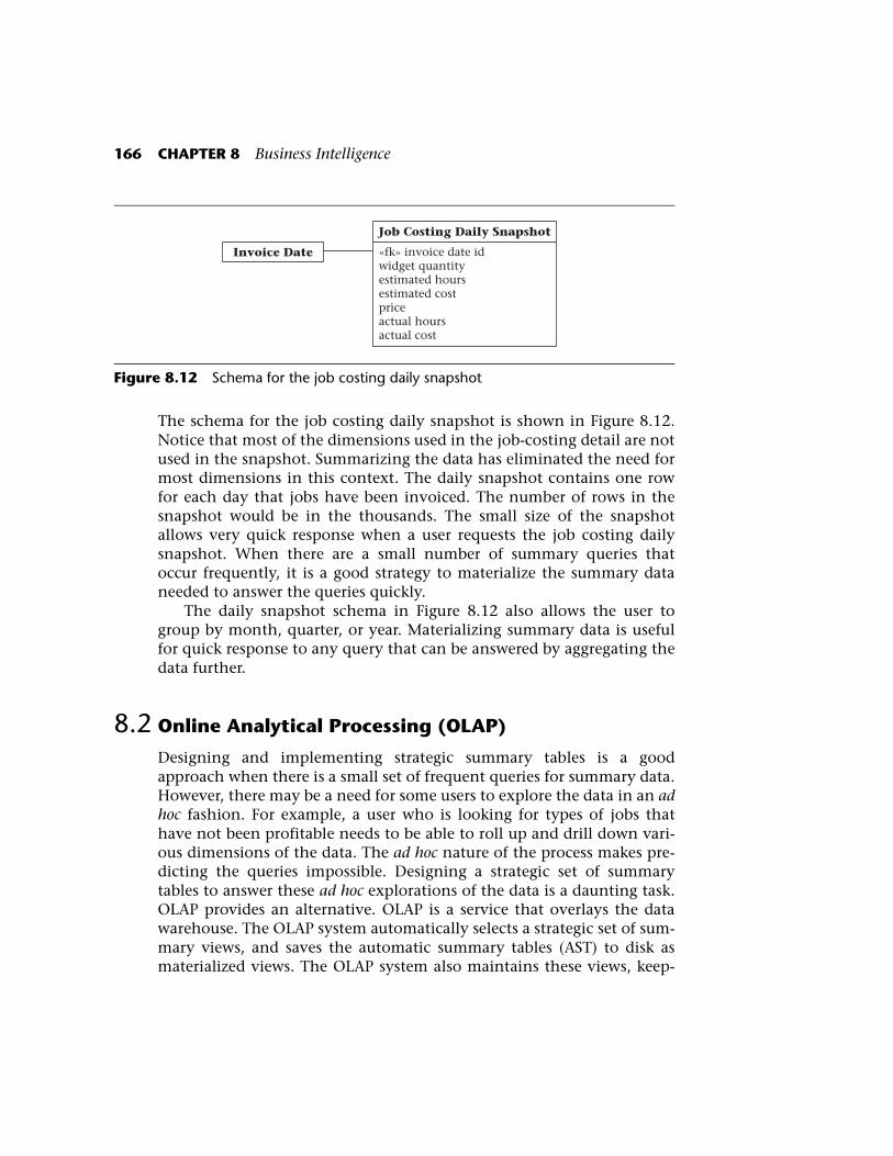
The schema for the job costing daily snapshot is shown in Figure 8.12.Notice that most of the dimensions used in the job-costing detail are notused in the snapshot. Summarizing the data has eliminated the need formost dimensions in this context. The daily snapshot contains one rowfor each day that jobs have been invoiced. The number of rows in thesnapshot would be in the thousands. The small size of the snapshotallows very quick response when a user requests the job costing dailysnapshot. When there are a small number of summary queries thatoccur frequently, it is a good strategy to materialize the summary dataneeded to answer the queries quickly.

The daily snapshot schema in Figure 8.12 also allows the user togroup by month, quarter, or year. Materializing summary data is usefulfor quick response to any query that can be answered by aggregating thedata further.

8.2 Online Analytical Processing (OLAP)

Designing and implementing strategic summary tables is a goodapproach when there is a small set of frequent queries for summary data.However, there may be a need for some users to explore the data in an adhoc fashion. For example, a user who is looking for types of jobs thathave not been profitable needs to be able to roll up and drill down vari-ous dimensions of the data. The ad hoc nature of the process makes pre-dicting the queries impossible. Designing a strategic set of summarytables to answer these ad hoc explorations of the data is a daunting task.OLAP provides an alternative. OLAP is a service that overlays the datawarehouse. The OLAP system automatically selects a strategic set of sum-mary views, and saves the automatic summary tables (AST) to disk asmaterialized views. The OLAP system also maintains these views, keep-

Figure 8.12 Schema for the job costing daily snapshot

«fk» invoice date idwidget quantityestimated hoursestimated costpriceactual hoursactual cost

Job Costing Daily Snapshot

Invoice Date

8.2 Online Analytical Processing (OLAP) 167

ing them in step with the fact tables as new data arrives. When a userrequests summary data, the OLAP system figures out which AST can beused for a quick response to the given query. OLAP systems are a goodsolution when there is a need for ad hoc exploration of summary infor-mation based on large amounts of data residing in a data warehouse.

OLAP systems automatically select, maintain, and use the ASTs.Thus, an OLAP system effectively does some of the design work auto-matically. This section covers some of the issues that arise in building anOLAP engine, and some of the possible solutions. If you use an OLAPsystem, the vendor delivers the OLAP engine to you. The issues and solu-tions discussed here are not items that you need to resolve. Our goalhere is to remove some of the mystery about what an OLAP system isand how it works.

8.2.1 The Exponential Explosion of Views

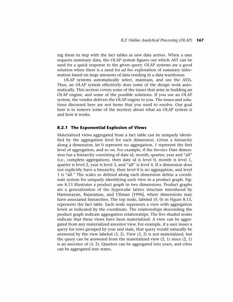
Materialized views aggregated from a fact table can be uniquely identi-fied by the aggregation level for each dimension. Given a hierarchyalong a dimension, let 0 represent no aggregation, 1 represent the firstlevel of aggregation, and so on. For example, if the Invoice Date dimen-sion has a hierarchy consisting of date id, month, quarter, year and “all”(i.e., complete aggregation), then date id is level 0, month is level 1,quarter is level 2, year is level 3, and “all” is level 4. If a dimension doesnot explicitly have a hierarchy, then level 0 is no aggregation, and level1 is “all.” The scales so defined along each dimension define a coordi-nate system for uniquely identifying each view in a product graph. Fig-ure 8.13 illustrates a product graph in two dimensions. Product graphsare a generalization of the hypercube lattice structure introduced byHarinarayan, Rajaraman, and Ullman [1996], where dimensions mayhave associated hierarchies. The top node, labeled (0, 0) in Figure 8.13,represents the fact table. Each node represents a view with aggregationlevels as indicated by the coordinate. The relationships descending theproduct graph indicate aggregation relationships. The five shaded nodesindicate that these views have been materialized. A view can be aggre-gated from any materialized ancestor view. For example, if a user issues aquery for rows grouped by year and state, that query would naturally beanswered by the view labeled (3, 2). View (3, 2) is not materialized, butthe query can be answered from the materialized view (2, 1) since (2, 1)is an ancestor of (3, 2). Quarters can be aggregated into years, and citiescan be aggregated into states.


The central issue challenging the design of OLAP systems is theexponential explosion of possible views as the number of dimensionsincreases. The Calendar dimension in Figure 8.13 has five levels of hier-archy, and the Customer dimension has four levels of hierarchy. Theuser may choose any level of aggregation along each dimension. Thenumber of possible views is the product of the number of hierarchicallevels along each dimension. The number of possible views for theexample in Figure 8.13 is 5 × 4 = 20. Let d be the number of dimensionsin a data warehouse. Let hi be the number of hierarchical levels indimension i. The general equation for calculating the number of possi-ble views is given by Equation 8.1.

Possible views = 8.1

If we express Equation 8.1 in different terms, the problem of expo-nential explosion becomes more apparent. Let g be the geometric mean

Figure 8.13 Product graph labeled with aggregation level coordinates

Calendar Dimension(first dimension)

0: date id1: month2: quarter3: year4: all

Customer Dimension(second dimension)

0: cust id1: city2: state3: all

(0, 0)

(1, 0) (0, 1)

(1, 1) (0, 2)

(1, 2) (0, 3)

(1, 3)

(2, 0)

(2, 1)

(2, 2)

(2, 3)

(3, 0)

(3, 1)

(3, 2)

(3, 3)

(4, 0)

(4, 1)

(4, 2)

(4, 3)

Fact Table

hi

i 1=

d

∏


of the number of hierarchical levels in the dimensions. Then Equation8.1 becomes Equation 8.2.

Possible views = gd 8.2

As dimensionality increases linearly, the number of possible viewsexplodes exponentially. If g = 5 and d = 5, there are 55 = 3,125 possibleviews. Thus if d = 10, then there are 510 = 9,765,625 possible views.OLAP administrators need the freedom to scale up the dimensionality oftheir data warehouses. Clearly the OLAP system cannot create and main-tain all possible views as dimensionality increases. The design of OLAPsystems must deliver quick response while maintaining a system withinthe resource limitations. Typically, a strategic subset of views must beselected for materialization.

8.2.2 Overview of OLAP

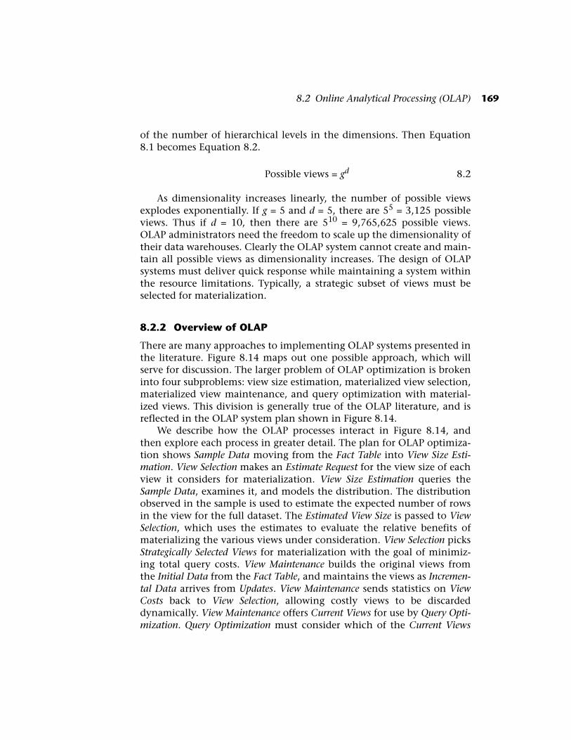
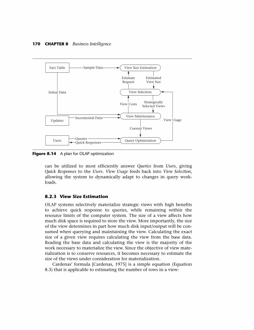
There are many approaches to implementing OLAP systems presented inthe literature. Figure 8.14 maps out one possible approach, which willserve for discussion. The larger problem of OLAP optimization is brokeninto four subproblems: view size estimation, materialized view selection,materialized view maintenance, and query optimization with material-ized views. This division is generally true of the OLAP literature, and isreflected in the OLAP system plan shown in Figure 8.14.

We describe how the OLAP processes interact in Figure 8.14, andthen explore each process in greater detail. The plan for OLAP optimiza-tion shows Sample Data moving from the Fact Table into View Size Esti-mation. View Selection makes an Estimate Request for the view size of eachview it considers for materialization. View Size Estimation queries theSample Data, examines it, and models the distribution. The distributionobserved in the sample is used to estimate the expected number of rowsin the view for the full dataset. The Estimated View Size is passed to ViewSelection, which uses the estimates to evaluate the relative benefits ofmaterializing the various views under consideration. View Selection picksStrategically Selected Views for materialization with the goal of minimiz-ing total query costs. View Maintenance builds the original views fromthe Initial Data from the Fact Table, and maintains the views as Incremen-tal Data arrives from Updates. View Maintenance sends statistics on ViewCosts back to View Selection, allowing costly views to be discardeddynamically. View Maintenance offers Current Views for use by Query Opti-mization. Query Optimization must consider which of the Current Views


can be utilized to most efficiently answer Queries from Users, givingQuick Responses to the Users. View Usage feeds back into View Selection,allowing the system to dynamically adapt to changes in query work-loads.

8.2.3 View Size Estimation

OLAP systems selectively materialize strategic views with high benefitsto achieve quick response to queries, while remaining within theresource limits of the computer system. The size of a view affects howmuch disk space is required to store the view. More importantly, the sizeof the view determines in part how much disk input/output will be con-sumed when querying and maintaining the view. Calculating the exactsize of a given view requires calculating the view from the base data.Reading the base data and calculating the view is the majority of thework necessary to materialize the view. Since the objective of view mate-rialization is to conserve resources, it becomes necessary to estimate thesize of the views under consideration for materialization.

Cardenas’ formula [Cardenas, 1975] is a simple equation (Equation8.3) that is applicable to estimating the number of rows in a view:

Figure 8.14 A plan for OLAP optimization

Fact Table

Updates

Sample Data

EstimatedView Size

StrategicallySelected Views

Current Views

Incremental Data

QueriesQuick Responses

EstimateRequest

View Size Estimation

View Selection

View Maintenance

Initial Data

View Usage

Users Query Optimization

View Costs


Let n be the number of rows in the fact table.

Let v be the number of possible keys in the data space of the view.

Expected distinct values = v(1 – (1 – 1/v)n) 8.3

Cardenas’ formula assumes a uniform data distribution. However,many data distributions exist. The data distribution in the fact tableaffects the number of rows in a view. Cardenas’ formula is very quick,but the assumption of a uniform data distribution leads to gross overesti-mates of the view size when the data is actually clustered. Other meth-ods have been developed to model the effect of data distribution on thenumber of rows in a view.

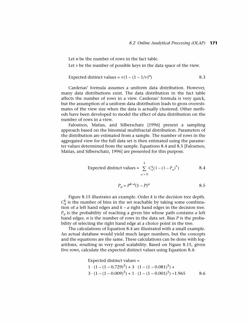
Faloutsos, Matias, and Silberschatz [1996] present a samplingapproach based on the binomial multifractal distribution. Parameters ofthe distribution are estimated from a sample. The number of rows in theaggregated view for the full data set is then estimated using the parame-ter values determined from the sample. Equations 8.4 and 8.5 [Faloutsos,Matias, and Silberschatz, 1996] are presented for this purpose.

Expected distinct values = 8.4

Pa = Pk–a(1 – P)a 8.5

Figure 8.15 illustrates an example. Order k is the decision tree depth.Ck

a is the number of bins in the set reachable by taking some combina-tion of a left hand edges and k – a right hand edges in the decision tree.Pa is the probability of reaching a given bin whose path contains a lefthand edges. n is the number of rows in the data set. Bias P is the proba-bility of selecting the right hand edge at a choice point in the tree.

The calculations of Equation 8.4 are illustrated with a small example.An actual database would yield much larger numbers, but the conceptsand the equations are the same. These calculations can be done with log-arithms, resulting in very good scalability. Based on Figure 8.15, givenfive rows, calculate the expected distinct values using Equation 8.4:

Expected distinct values =

1 ⋅ (1 – (1 – 0.729)5) + 3 ⋅ (1 – (1 – 0.081)5) +

3 ⋅ (1 – (1 – 0.009)5) + 1 ⋅ (1 – (1 – 0.001)5) ≈1.965 8.6

Cak 1 1 Pa–( )n

–( )a 0=

k

∑


The values of P and k can be estimated based on sample data. Thealgorithm used in [Faloutsos, Matias, and Silberschatz, 1996] has threeinputs: the number of rows in the sample, the frequency of the mostcommonly occurring value, and the number of distinct aggregate rowsin the sample. The value of P is calculated based on the frequency of themost commonly occurring value. They begin with:

k = ⎡Log2(Distinct rows in sample)⎤ 8.7

and then adjust k upwards, recalculating P until a good fit to the numberof distinct rows in the sample is found.

Other distribution models can be utilized to predict the size of a viewbased on sample data. For example, the use of the Pareto distributionmodel has been explored [Nadeau and Teorey, 2003]. Another possibilityis to find the best fit to the sample data for multiple distribution models,calculate which model is most likely to produce the given sample data,and then use that model to predict the number of rows for the full dataset. This would require calculation for each distribution model consid-ered, but should generally result in more accurate estimates.

Figure 8.15 Example of a binomial multifractal distribution tree

P = 0.9

0.9 0.9

0.9 0.9 0.9 0.9

0.1

0.1

0.1

0.1

0.1 0.1 0.1

0.7290.0810.081 0.0810.0090.009 0.0090.001

a = 2 leftsP2 = 0.009

a = 1 leftP1 = 0.081

a = 0 leftsP0 = 0.729

C = 1 binC = 3 bins32

C = 3 bins31

30

a = 3 leftsP3 = 0.001

C = 1 bin33


8.2.4 Selection of Materialized Views

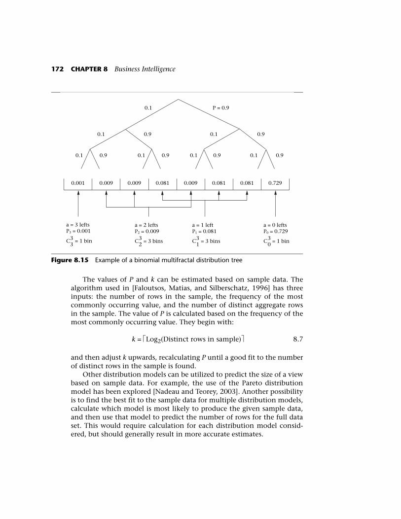
Most of the published works on the problem of materialized view selec-tion are based on the hypercube lattice structure [Harinarayan, Rajara-man, and Ullman, 1996]. The hypercube lattice structure is a special caseof the product graph structure, where the number of hierarchical levelsfor each dimension is two. Each dimension can either be included orexcluded from a given view. Thus, the nodes in a hypercube lattice struc-ture represent the power set of the dimensions.

Figure 8.16 illustrates the hypercube lattice structure with an exam-ple [Harinarayan, Rajaraman, and Ullman, 1996]. Each node of the lat-tice structure represents a possible view. Each node is labeled with the setof dimensions in the “group by” list for that view. The numbers associ-ated with the nodes represent the number of rows in the view. Thesenumbers are normally derived from a view size estimation algorithm, asdiscussed in Section 8.2.3. However, the numbers in Figure 8.16 followthe example as given by Harinarayan et al. [1996]. The relationshipsbetween nodes indicate which views can be aggregated from otherviews. A given view can be calculated from any materialized ancestorview.

We refer to the algorithm for selecting materialized views introducedby Harinarayan et al. [1996] as HRU. The initial state for HRU has onlythe fact table materialized. HRU calculates the benefit of each possibleview during each iteration, and selects the most beneficial view formaterialization. Processing continues until a predetermined number ofmaterialized views is reached.

Figure 8.16 Example of a hypercube lattice structure [Harinarayan et al. 1996]

c = Customerp = Parts = Supplier

{p, s} 0.8M {c, s} 6M {c, p} 6M

{s} 0.01M {p} 0.2M {c} 0.1M

{ } 1

Fact Table

{c, p, s} 6M


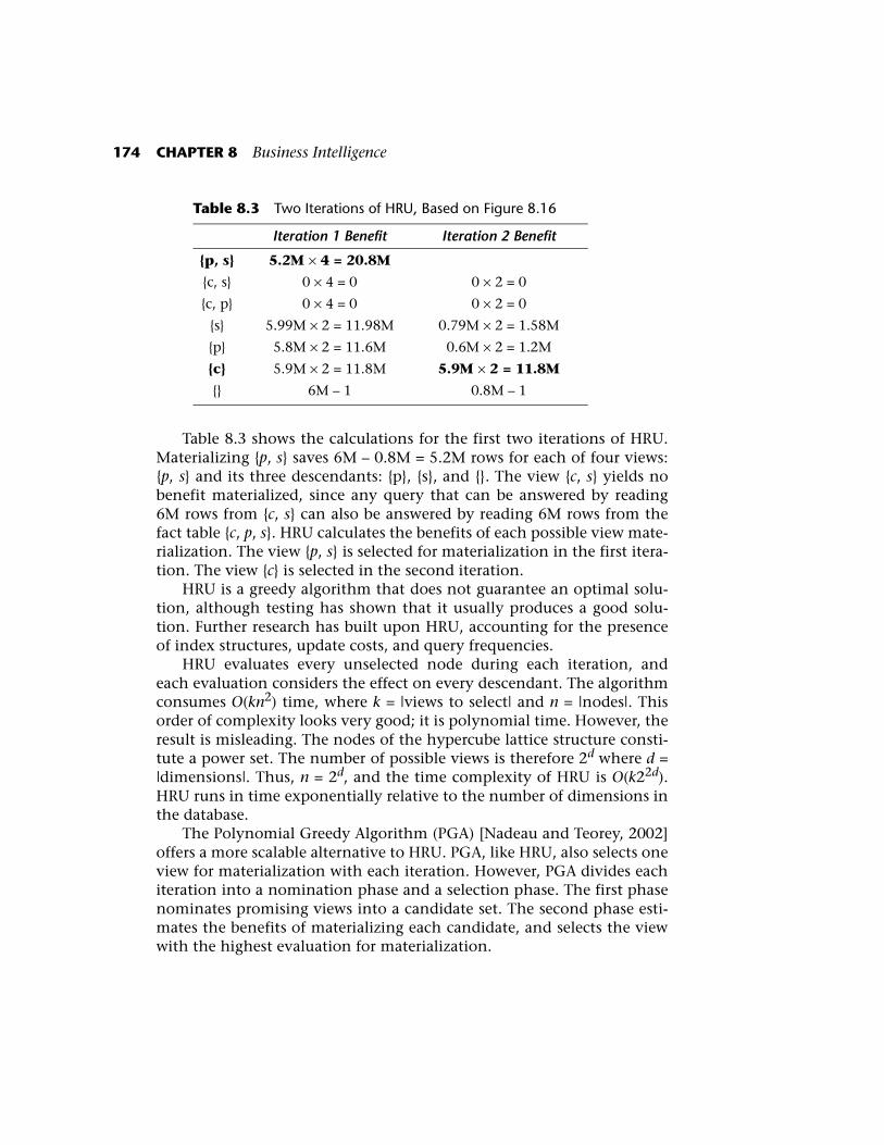
Table 8.3 shows the calculations for the first two iterations of HRU.Materializing {p, s} saves 6M – 0.8M = 5.2M rows for each of four views:{p, s} and its three descendants: {p}, {s}, and {}. The view {c, s} yields nobenefit materialized, since any query that can be answered by reading6M rows from {c, s} can also be answered by reading 6M rows from thefact table {c, p, s}. HRU calculates the benefits of each possible view mate-rialization. The view {p, s} is selected for materialization in the first itera-tion. The view {c} is selected in the second iteration.

HRU is a greedy algorithm that does not guarantee an optimal solu-tion, although testing has shown that it usually produces a good solu-tion. Further research has built upon HRU, accounting for the presenceof index structures, update costs, and query frequencies.

HRU evaluates every unselected node during each iteration, andeach evaluation considers the effect on every descendant. The algorithmconsumes O(kn2) time, where k = |views to select| and n = |nodes|. Thisorder of complexity looks very good; it is polynomial time. However, theresult is misleading. The nodes of the hypercube lattice structure consti-tute a power set. The number of possible views is therefore 2d where d =|dimensions|. Thus, n = 2d, and the time complexity of HRU is O(k22d).HRU runs in time exponentially relative to the number of dimensions inthe database.

The Polynomial Greedy Algorithm (PGA) [Nadeau and Teorey, 2002]offers a more scalable alternative to HRU. PGA, like HRU, also selects oneview for materialization with each iteration. However, PGA divides eachiteration into a nomination phase and a selection phase. The first phasenominates promising views into a candidate set. The second phase esti-mates the benefits of materializing each candidate, and selects the viewwith the highest evaluation for materialization.

Table 8.3 Two Iterations of HRU, Based on Figure 8.16

Iteration 1 Benefit Iteration 2 Benefit

{p, s}

{c, s}

{c, p}

{s}

{p}

{c}

{}

5.2M × 4 = 20.8M

0 × 4 = 0

0 × 4 = 0

5.99M × 2 = 11.98M

5.8M × 2 = 11.6M

5.9M × 2 = 11.8M

6M – 1

0 × 2 = 0

0 × 2 = 0

0.79M × 2 = 1.58M

0.6M × 2 = 1.2M

5.9M × 2 = 11.8M

0.8M – 1


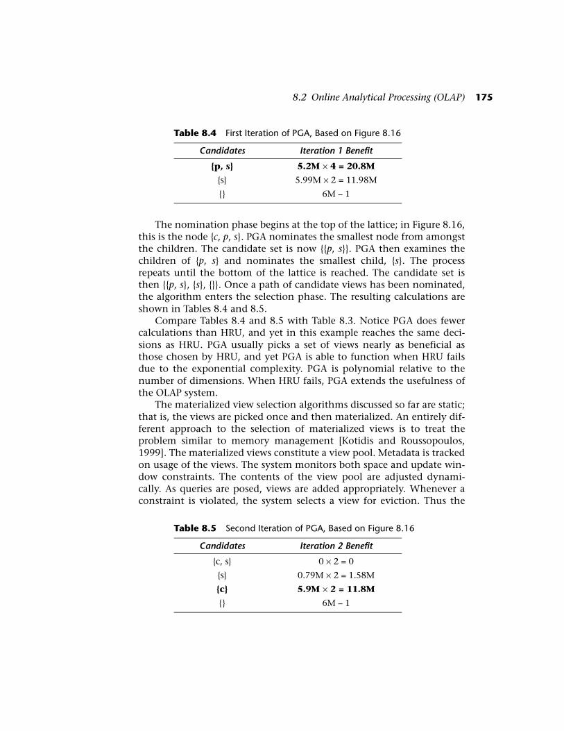
The nomination phase begins at the top of the lattice; in Figure 8.16,this is the node {c, p, s}. PGA nominates the smallest node from amongstthe children. The candidate set is now {{p, s}}. PGA then examines thechildren of {p, s} and nominates the smallest child, {s}. The processrepeats until the bottom of the lattice is reached. The candidate set isthen {{p, s}, {s}, {}}. Once a path of candidate views has been nominated,the algorithm enters the selection phase. The resulting calculations areshown in Tables 8.4 and 8.5.

Compare Tables 8.4 and 8.5 with Table 8.3. Notice PGA does fewercalculations than HRU, and yet in this example reaches the same deci-sions as HRU. PGA usually picks a set of views nearly as beneficial asthose chosen by HRU, and yet PGA is able to function when HRU failsdue to the exponential complexity. PGA is polynomial relative to thenumber of dimensions. When HRU fails, PGA extends the usefulness ofthe OLAP system.

The materialized view selection algorithms discussed so far are static;that is, the views are picked once and then materialized. An entirely dif-ferent approach to the selection of materialized views is to treat theproblem similar to memory management [Kotidis and Roussopoulos,1999]. The materialized views constitute a view pool. Metadata is trackedon usage of the views. The system monitors both space and update win-dow constraints. The contents of the view pool are adjusted dynami-cally. As queries are posed, views are added appropriately. Whenever aconstraint is violated, the system selects a view for eviction. Thus the

Table 8.4 First Iteration of PGA, Based on Figure 8.16

Candidates Iteration 1 Benefit

{p, s}

{s}

{}

5.2M × 4 = 20.8M

5.99M × 2 = 11.98M

6M – 1

Table 8.5 Second Iteration of PGA, Based on Figure 8.16

Candidates Iteration 2 Benefit

{c, s}

{s}

{c}

{}

0 × 2 = 0

0.79M × 2 = 1.58M

5.9M × 2 = 11.8M

6M – 1


view pool can improve as more usage statistics are gathered. This is aself-tuning system that adjusts to changing query patterns.

The static and dynamic approaches complement each other andshould be integrated. Static approaches run fast from the beginning, butdo not adapt. Dynamic view selection begins with an empty view pool,and therefore yields slow response times when a data warehouse is firstloaded; however, it is adaptable and improves over time. The comple-mentary nature of these two approaches has influenced our design planin Figure 8.14, as indicated by Queries feeding back into View Selection.

8.2.5 View Maintenance

Once a view is selected for materialization, it must be computed andstored. When the base data is updated, the aggregated view must also beupdated to maintain consistency between views. The original view mate-rialization and the incremental updates are both considered as viewmaintenance in Figure 8.14. The efficiency of view maintenance isgreatly affected by the data structures implementing the view. OLAP sys-tems are multidimensional, and fact tables contain large numbers ofrows. The access methods implementing the OLAP system must meetthe challenges of high dimensionality in combination with large rowcounts. The physical structures used are deferred to volume two, whichcovers physical design.

Most of the research papers in the area of view maintenance assumethat new data is periodically loaded with incremental data during desig-nated update windows. Typically, the OLAP system is made unavailableto the users while the incremental data is loaded in bulk, taking advan-tage of the efficiencies of bulk operations. There is a down side to defer-ring the loading of incremental data until the next update window. Ifthe data warehouse receives incremental data once a day, then there is aone-day latency period.

There is currently a push in the industry to accommodate dataupdates close to real time, keeping the data warehouse in step with theoperational systems. This is sometimes referred to as “active warehous-ing” and “real-time analytics.” The need for data latency of only a fewminutes presents new problems. How can very large data structures bemaintained efficiently with a trickle feed? One solution is to have a sec-ond set of data structures with the same schema as the data warehouse.This second set of data structures acts as a holding tank for incrementaldata, and is referred to as a delta cube in OLAP terminology. The opera-tional systems feed into the delta cube, which is small and efficient for


quick incremental changes. The data cube is updated periodically fromthe delta cube, taking advantage of bulk operation efficiencies. Whenthe user queries the OLAP system, the query can be issued against boththe data cube and the delta cube to obtain an up-to-date result. The deltacube is hidden from the user. What the user sees is an OLAP system thatis nearly current with the operational systems.

8.2.6 Query Optimization

When a query is posed to an OLAP system, there may be multiple mate-rialized views available that could be used to compute the result. Forexample, if we have the situation represented in Figure 8.13, and a userissues a query to group rows by month and state, that query is naturallyanswered from the view labeled (1, 2). However, since (1, 2) is not mate-rialized, we need to find a materialized ancestor to obtain the data.There are three such nodes in the product graph of Figure 8.13. Thequery can be answered from nodes (0, 0), (1, 0), or (0, 2). With the possi-bility of answering queries from alternative sources, the optimizationissue arises as to which source is the most efficient for the given query.Most existing research focuses on syntactic approaches. The possiblequery translations are carried out, alternative query costs are estimated,and what appears to be the best plan is executed. Another approach is toquery a metadata table containing information on the materializedviews to determine the best view to query against, and then translate theoriginal SQL query to use the best view.

Database systems contain metadata tables that hold data about thetables and other structures used by the system. The metadata tables facil-itate the system in its operations. Here’s an example where a metadata

Table 8.6 Example of Materialized View Metadata

Dimensions

Calendar Customer Blocks ViewID

0 0 10,000,000 1

0 2 50,000 3

0 3 1,000 5

1 0 300,000 2

2 1 10,000 4


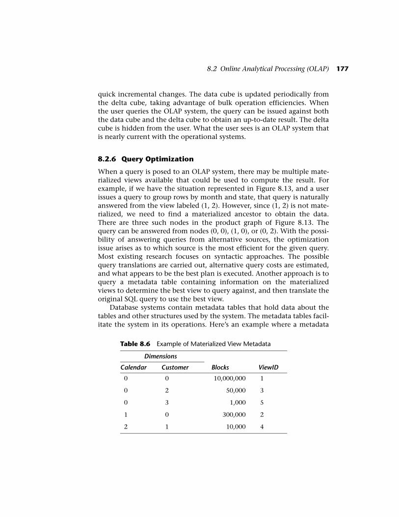
table can facilitate the process of finding the best view to answer a queryin an OLAP system. The coordinate system defined by the aggregationlevels forms the basis for organizing the metadata for tracking the mate-rialized views. Table 8.6 displays the metadata for the materialized viewsshaded in Figure 8.13. The two dimensions labeled Calendar and Cus-tomer form the composite key. The Blocks column tracks the actual num-ber of blocks in each materialized view. The ViewID column is used toidentify the associated materialized view. The implementation storesmaterialized views as tables where the value of the ViewID forms part ofthe table name. For example, the row with ViewID = 3 contains informa-tion on the aggregated view that is materialized as table AST3 (short forautomatic summary table 3).

Observe the general pattern in the coordinates of the views in theproduct graph with regard to ancestor relationships. Let Value(V, d) rep-resent a function that returns the aggregation level for view V alongdimension d. For any two views Vi and Vj where Vi ≠ Vj, Vi is an ancestorof Vj if and only if for every dimension d of the composite key, Value(Vi,d) ≤ Value(Vj, d). This pattern in the keys can be utilized to identifyancestors of a given view by querying the metadata. The semantics ofthe product graph are captured by the metadata, permitting the OLAPsystem to search semantically for the best materialized ancestor view byquerying the metadata table. After the best materialized view is deter-mined, the OLAP system can rewrite the original query to utilize the bestmaterialized view, and proceed.

8.3 Data Mining

Two general approaches are used to extract knowledge from a database.First, a user may have a hypothesis to verify or disprove. This type ofanalysis is done with standard database queries and statistical analysis.The second approach to extracting knowledge is to have the computersearch for correlations in the data, and present promising hypotheses tothe user for consideration. The methods included here are data miningtechniques developed in the fields of Machine Learning and KnowledgeDiscovery.

Data mining algorithms attempt to solve a number of commonproblems. One general problem is categorization: given a set of caseswith known values for some parameters, classify the cases. For example,given observations of patients, suggest a diagnosis. Another generalproblem type is clustering: given a set of cases, find natural groupings ofthe cases. Clustering is useful, for example, in identifying market seg-

8.3 Data Mining 179

ments. Association rules, also known as market basket analyses, areanother common problem. Businesses sometimes want to know whatitems are frequently purchased together. This knowledge is useful, forexample, when decisions are made about how to lay out a grocery store.There are many types of data mining available. Han and Kamber [2001]cover data mining in the context of data warehouses and OLAP systems.Mitchell [1997] is a rich resource, written from the machine learningperspective. Witten and Frank [2000] give a survey of data mining, alongwith freeware written in Java available from the Weka Web site [http://www.cs.waikato.ac.nz/ml/weka]. The Weka Web site is a good option forthose who wish to experiment with and modify existing algorithms. Themajor database vendors also offer data mining packages that functionwith their databases.

Due to the large scope of data mining, we focus on two forms of datamining: forecasting and text mining.

8.3.1 Forecasting

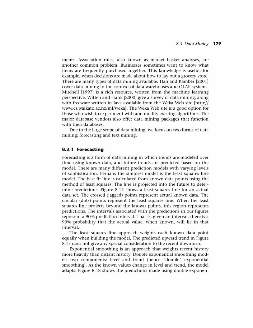
Forecasting is a form of data mining in which trends are modeled overtime using known data, and future trends are predicted based on themodel. There are many different prediction models with varying levelsof sophistication. Perhaps the simplest model is the least squares linemodel. The best fit line is calculated from known data points using themethod of least squares. The line is projected into the future to deter-mine predictions. Figure 8.17 shows a least squares line for an actualdata set. The crossed (jagged) points represent actual known data. Thecircular (dots) points represent the least squares line. When the leastsquares line projects beyond the known points, this region representspredictions. The intervals associated with the predictions in our figuresrepresent a 90% prediction interval. That is, given an interval, there is a90% probability that the actual value, when known, will lie in thatinterval.

The least squares line approach weights each known data pointequally when building the model. The predicted upward trend in Figure8.17 does not give any special consideration to the recent downturn.

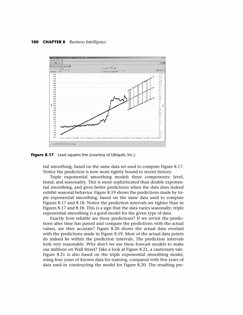
Exponential smoothing is an approach that weights recent historymore heavily than distant history. Double exponential smoothing mod-els two components: level and trend (hence “double” exponentialsmoothing). As the known values change in level and trend, the modeladapts. Figure 8.18 shows the predictions made using double exponen-


tial smoothing, based on the same data set used to compute Figure 8.17.Notice the prediction is now more tightly bound to recent history.

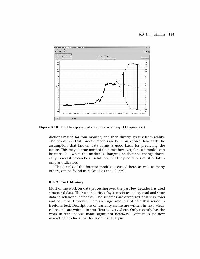
Triple exponential smoothing models three components: level,trend, and seasonality. This is more sophisticated than double exponen-tial smoothing, and gives better predictions when the data does indeedexhibit seasonal behavior. Figure 8.19 shows the predictions made by tri-ple exponential smoothing, based on the same data used to computeFigures 8.17 and 8.18. Notice the prediction intervals are tighter than inFigures 8.17 and 8.18. This is a sign that the data varies seasonally; tripleexponential smoothing is a good model for the given type of data.

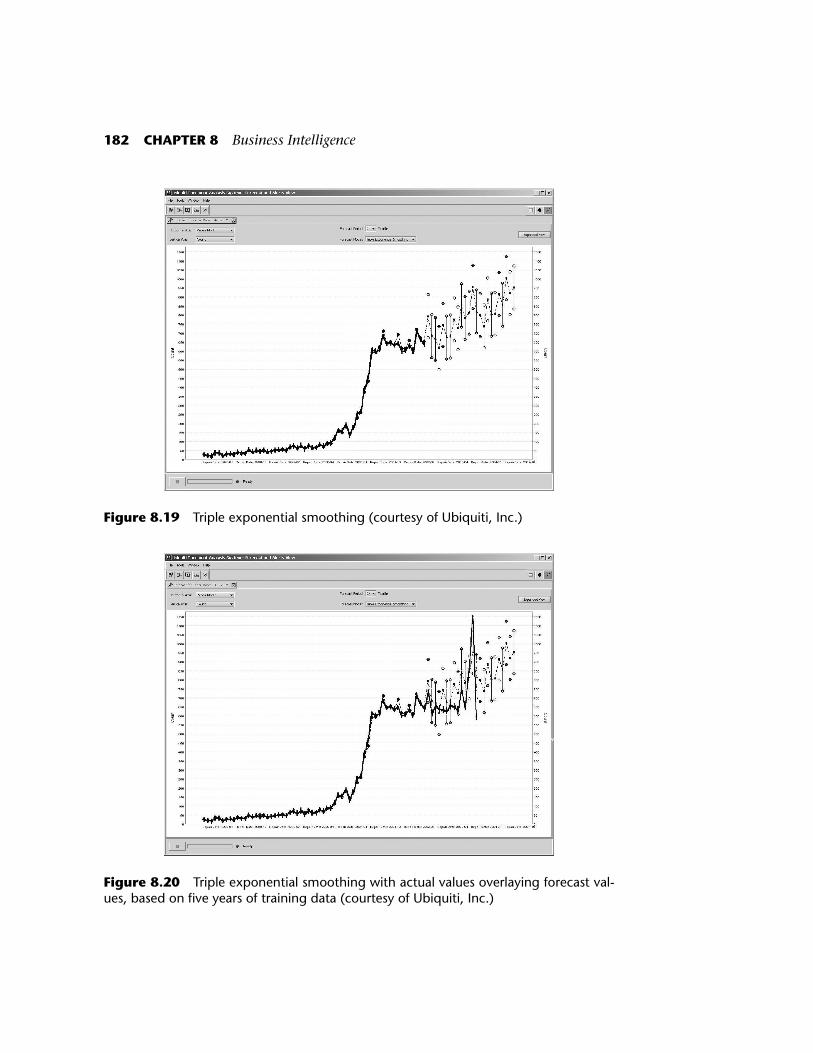
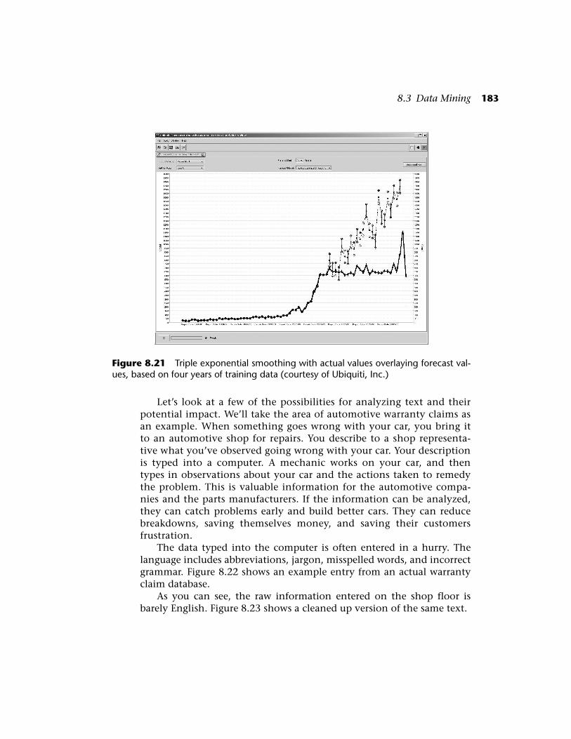
Exactly how reliable are these predictions? If we revisit the predic-tions after time has passed and compare the predictions with the actualvalues, are they accurate? Figure 8.20 shows the actual data overlaidwith the predictions made in Figure 8.19. Most of the actual data pointsdo indeed lie within the prediction intervals. The prediction intervalslook very reasonable. Why don’t we use these forecast models to makeour millions on Wall Street? Take a look at Figure 8.21, a cautionary tale.Figure 8.21 is also based on the triple exponential smoothing model,using four years of known data for training, compared with five years ofdata used in constructing the model for Figure 8.20. The resulting pre-

Figure 8.17 Least squares line (courtesy of Ubiquiti, Inc.)

8.3 Data Mining 181

dictions match for four months, and then diverge greatly from reality.The problem is that forecast models are built on known data, with theassumption that known data forms a good basis for predicting thefuture. This may be true most of the time; however, forecast models canbe unreliable when the market is changing or about to change drasti-cally. Forecasting can be a useful tool, but the predictions must be takenonly as indicators.

The details of the forecast models discussed here, as well as manyothers, can be found in Makridakis et al. [1998].

8.3.2 Text Mining

Most of the work on data processing over the past few decades has usedstructured data. The vast majority of systems in use today read and storedata in relational databases. The schemas are organized neatly in rowsand columns. However, there are large amounts of data that reside infreeform text. Descriptions of warranty claims are written in text. Medi-cal records are written in text. Text is everywhere. Only recently has thework in text analysis made significant headway. Companies are nowmarketing products that focus on text analysis.

Figure 8.18 Double exponential smoothing (courtesy of Ubiquiti, Inc.)


Figure 8.19 Triple exponential smoothing (courtesy of Ubiquiti, Inc.)

Figure 8.20 Triple exponential smoothing with actual values overlaying forecast val-ues, based on five years of training data (courtesy of Ubiquiti, Inc.)

8.3 Data Mining 183

Let’s look at a few of the possibilities for analyzing text and theirpotential impact. We’ll take the area of automotive warranty claims asan example. When something goes wrong with your car, you bring itto an automotive shop for repairs. You describe to a shop representa-tive what you’ve observed going wrong with your car. Your descriptionis typed into a computer. A mechanic works on your car, and thentypes in observations about your car and the actions taken to remedythe problem. This is valuable information for the automotive compa-nies and the parts manufacturers. If the information can be analyzed,they can catch problems early and build better cars. They can reducebreakdowns, saving themselves money, and saving their customersfrustration.

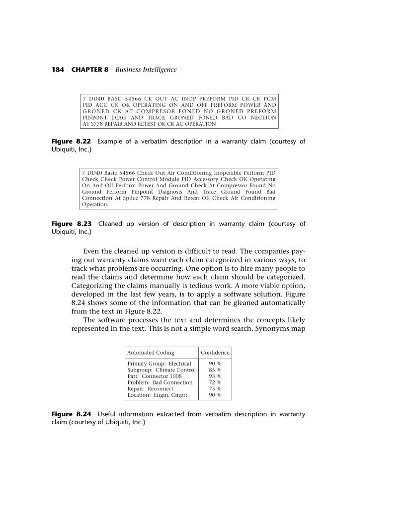
The data typed into the computer is often entered in a hurry. Thelanguage includes abbreviations, jargon, misspelled words, and incorrectgrammar. Figure 8.22 shows an example entry from an actual warrantyclaim database.

As you can see, the raw information entered on the shop floor isbarely English. Figure 8.23 shows a cleaned up version of the same text.

Figure 8.21 Triple exponential smoothing with actual values overlaying forecast val-ues, based on four years of training data (courtesy of Ubiquiti, Inc.)


Even the cleaned up version is difficult to read. The companies pay-ing out warranty claims want each claim categorized in various ways, totrack what problems are occurring. One option is to hire many people toread the claims and determine how each claim should be categorized.Categorizing the claims manually is tedious work. A more viable option,developed in the last few years, is to apply a software solution. Figure8.24 shows some of the information that can be gleaned automaticallyfrom the text in Figure 8.22.

The software processes the text and determines the concepts likelyrepresented in the text. This is not a simple word search. Synonyms map

Figure 8.22 Example of a verbatim description in a warranty claim (courtesy ofUbiquiti, Inc.)

Figure 8.23 Cleaned up version of description in warranty claim (courtesy ofUbiquiti, Inc.)

Figure 8.24 Useful information extracted from verbatim description in warrantyclaim (courtesy of Ubiquiti, Inc.)

7 DD40 BASC 54566 CK OUT AC INOP PREFORM PID CK CK PCM PID ACC CK OK OPERATING ON AND OFF PREFORM POWER AND GRONED CK AT COMPRESOR FONED NO GRONED PREFORM PINPONT DIAG AND TRACE GRONED FONED BAD CO NECTION AT S778 REPAIR AND RETEST OK CK AC OPERATION

7 DD40 Basic 54566 Check Out Air Conditioning Inoperable Perform PID Check Check Power Control Module PID Accessory Check OK Operating On And Off Perform Power And Ground Check At Compressor Found No Ground Perform Pinpoint Diagnosis And Trace Ground Found Bad Connection At Splice 778 Repair And Retest OK Check Air Conditioning Operation.

Primary Group: ElectricalSubgroup: Climate ControlPart: Connector 1008Problem: Bad ConnectionRepair: ReconnectLocation: Engin. Cmprt.

90 %85 %93 %72 %75 %90 %

Automated Coding Confidence

8.4 Summary 185

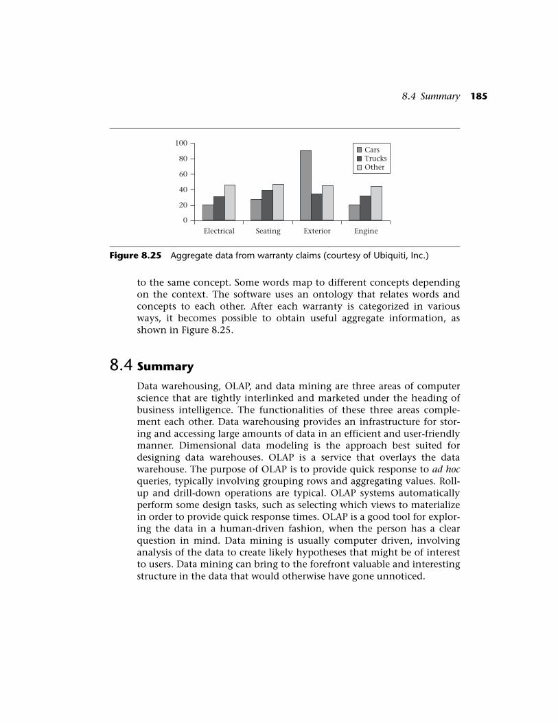
to the same concept. Some words map to different concepts dependingon the context. The software uses an ontology that relates words andconcepts to each other. After each warranty is categorized in variousways, it becomes possible to obtain useful aggregate information, asshown in Figure 8.25.

8.4 Summary

Data warehousing, OLAP, and data mining are three areas of computerscience that are tightly interlinked and marketed under the heading ofbusiness intelligence. The functionalities of these three areas comple-ment each other. Data warehousing provides an infrastructure for stor-ing and accessing large amounts of data in an efficient and user-friendlymanner. Dimensional data modeling is the approach best suited fordesigning data warehouses. OLAP is a service that overlays the datawarehouse. The purpose of OLAP is to provide quick response to ad hocqueries, typically involving grouping rows and aggregating values. Roll-up and drill-down operations are typical. OLAP systems automaticallyperform some design tasks, such as selecting which views to materializein order to provide quick response times. OLAP is a good tool for explor-ing the data in a human-driven fashion, when the person has a clearquestion in mind. Data mining is usually computer driven, involvinganalysis of the data to create likely hypotheses that might be of interestto users. Data mining can bring to the forefront valuable and interestingstructure in the data that would otherwise have gone unnoticed.

Figure 8.25 Aggregate data from warranty claims (courtesy of Ubiquiti, Inc.)

0

20

40

60

80

100

Electrical Seating Exterior Engine

CarsTrucksOther


8.5 Literature Summary

The evolution and principles of data warehouses can be found in Bar-quin and Edelstein [1997], Cataldo [1997], Chaudhuri and Dayal [1997],Gray and Watson [1998], Kimball and Ross [1998, 2002], and Kimballand Caserta [2004]. OLAP is discussed in Barquin and Edelstein [1997],Faloutsos, Matia, and Silberschatz [1996], Harinarayan, Rajaraman, andUllman [1996], Kotidis and Roussopoulos [1999], Nadeau and Teorey[2002 2003], Thomsen [1997], and data mining principles and tools canbe found in Han and Kamber [2001], Makridakis, Wheelwright, andHyndman [1998], Mitchell [1997], The University of Waikato [2005],Witten and Frank [2000], among many others.

business intelligence - cdn.ttgtmedia.com · warehousing, olap, and data mining as business...

Documents