35

BUYING VS. RENTING FARM LAND

Arthur Lerner’

Section 1 . Objective

In a recent University publication [ l ] on farm investment decisions, a formula was presented for the purpose of comparing the costs of owning land with rental costs. The formula given was:

100 C = V i + T - V r ~

(100 - I )

where C = annual cost of owning V = current market price (of land) T = property taxes, maintenance costs, etc. I = marginal income tax rate (per cent) i = interest rate (decimal fraction per annum) r = expected rate of change in land value (decimal fraction per annum)

A rider was added stating, “The formula is accurate for a one-year projection. A more complicated formula is needed for long-run projections.”

The object of this note is to develop the “more complicated” formula needed to compare the cost of owning a piece of land with a rental contract for a given number of years. This may be done by comparing the present value of the costs of owning the land with the present value of the rents for those years. The re- quired formula, Equation (8) , is derived in the next Section.

Section 2. Calculations To facilitate the calculation we may use a subscript, j, to represent the value

of each variable for the year j, (j = 1 . . . n), except that Vj will be the market price of the land at the beginning of year j. We may also use the following variables :

(brackets added for clarification)

h = expected rate of change of T (decimal fraction per annum).

g = - loo tfie “grossing up” ratio for income tax purposes. 100 - I

R = annual rent required as an alternative to buying. C‘”) = annual rental which would be equal to the equivalent annual cost

of owning the land for n years.

The cost of owning land for year j may then be written:

C, = Vj(ij - rjgj) + Tj (j = 1 . . . n) (2) If there is a capital gains tax at a lower rate than income tax, as in Canada

and the US., I, will equal the difference between marginal income tax rate and marginal capital gains tax rate expected for year j ; then gj will change correspondingly.

* University of Guclph.

Canadian Journal of Agricultural Economics 24(3), 1976

36

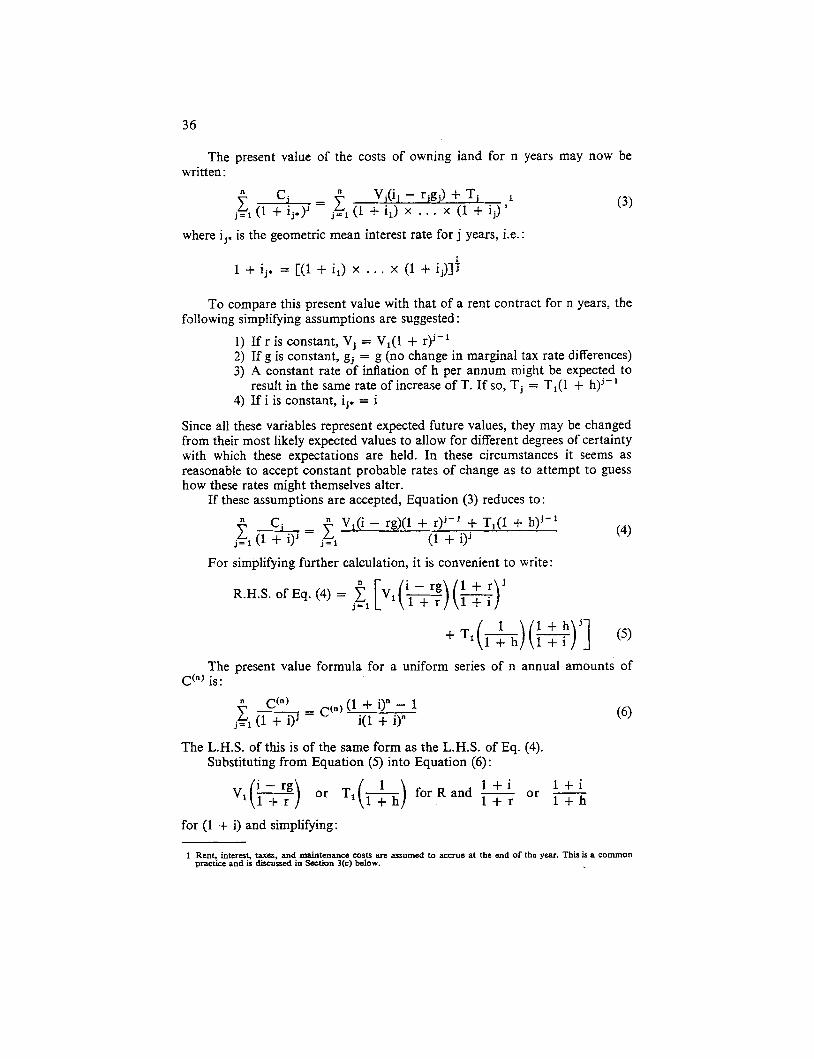
The present value of the costs of owning land for n years may now be written :

Cj = Vj(ij - rjgj) + T, j=l i (1 + ij*)’ j= l (1 + il) x . . . x (1 + ij) ’ (3)

where ij. is the geometric mean interest rate for j years, i.e. :

1 1 + ij, = [(l + il) x . . . x (1 + ij)]i

To compare this present value with that of a rent contract for n years, the following simplifying assumptions are suggested :

1) If r is constant, Vj = V,(1 + r)j-’ 2) If g is constant, gj = g (no change in marginal tax rate differences) 3) A constant rate of inflation of h per annum might be expected to

result in the same rate of increase of T. If so, T j = T,(1 + h)j-’ 4) If i is constant, ij, = i

Since all these variables represent expected future values, they may be changed from their most likely expected values to allow for different degrees of certainty with which these expectations are held. In these circumstances it seems as reasonable to accept constant probable rates of change as to attempt to guess how these rates might themselves alter.

If these assumptions are accepted, Equation (3) reduces to:

(4) Ci .=f V,(i - rg)(l + r)j-’ + T,(1 + h)j-’

For simplifying further calculation, it is convenient to write : j=l f: (1 + i)’ j=l (1 + i)’

R.H.S. of Eq. (4) = j = 1

The present value formula for a uniform series of n annual amounts of C‘”) is:

c ( n )

j=l i (1 + i)j - c ( n ) (1 + i>” - 1

i(l + i)”

The L.H.S. of this is of the same form as the L.H.S. of Eq. (4). Substituting from Equation ( 5 ) into Equation (6) :

l + i o r - l + i V l ( 3 ) or T1(&) for R and - l + r l + h

for (1 + i) and simplifying:

1 Rent, interest, taxes, and maintenance costs arc assumed to accrue at the end of the year. This is a common practice and is discussed in Section 3(c) below.

37

1 (1 + i)” - (1 + r)” (I + i)“ R.H.S. of Eq. (4) = V,(i - rg)( z)

This present value can now be compared with that of a series of n annual rents R (payable at the end of each year)2. By putting the R.H.S. of Equation (6) equal to that of Equation (7) and dividing:

i (1 + i)“ - (1 + r)” c(”) = vl(i - rg)( 1 - r -) ( l + i ) ” - 1

(8) i)” - (1 + h)” + T, ( + (1 + i)” - 1

This is the annual rental which would be equal to the equivalent annual cost of owning the land for n years. If n = 1, it reduces to: C(”) = V,(i - rg) + T1 which is equivalent to Equation (1). The decision rule which results is: If R(rent required) exceeds C‘”), buy; if C‘”) exceeds R, rent.

Section 3. Some Further Considerations (a) Property Taxes.

It will be noted that if the rent contract provides for property taxes, maintenance costs, etc., to be paid by the tenant, the element containing T can be omitted from all the equations, while, if they are paid by the owner but the rise in land values is’not expected to be accompanied by a rise in these costs, T remains constant. (b) A Perpetual Rent.

As n approaches infinity,

(1 + i)” - (1 + r)” and (1 + i)” - (1 + h)” (1 + i)” - 1 (1 + i)” - 1

approach 13, so that a perpetual rent equivalent to the cost of owning the land would be given by :

If T is excluded from the calculations and capital gains and income are taxed at equal rates, g = 1 and Equation (9) reduces to: = Vli, which might seem strange at first sight, since r, the expected rate of increase of V, does not appear. The explanation is, of course, that by contracting for a perpetual rent the owner gives up to the tenant his right to realize the expected capital gain. Clearly this right will be discounted by raising its present value, V,. Thus if a property is expected to yield constant annual earnings of E, then Y, its present value, would be Eli and a perpetual annual rent of a of the same present value

2 see fwtnotc 1. 3 Strictly, if r and h exceed i, the expression approaches - m and the rent (equal to cost of owning land) is negative.

38

would be equal to r, from initial earnings of El, the present value would be:

= Ti. But if the earnings were expected to increase at rate

Hence, if E = E, i - - i" R - Vli = V-= R-. I - r i - r

It will be observed that Equations (8) and (9) could easily be adapted to compare the relative values of growth stocks, debentures, perpetual bonds and other forms of property, for investors with different marginal tax rates. (c) Adjustments for payments other than at the end of each year.

The equations given so far can be calculated simply by using the tables to be found in any ordinary book of interest tables. This is perfectly satisfactory if the assumptions on which they are based are correct. As indicated in footnote 1, this means that interest, taxes, costs and rents are all paid at the end of each year. If, however, some or all of them are paid at the beginning of the year or at specified intervals such as monthly or quarterly, an appropriate adjustment must be made to Equation (P), which is the formula to the derivation of which this paper was directed, or to Equation (1). The relative importance and method of calculation of such adjustments is discussed in an earlier article [2].

If the rent is payable at the beginning of the year, while all other costs accrue at the end, the R.H.S. of Equation (8) or Equation (1) must be divided by (1 + i). If interest payments, taxes, costs and rents are all paid in the same num- ber of instalments during the year, the adjustments cancel out and the equation holds. This can never be completely accurate, since the increase in value of the land can only accrue at the end of the year and income tax credits against interest payments and other costs usually accrue at the end of the year. It therefore becomes necessary to multiply each of the elements, C'"), i and T, by a multiplier which depends on the number of equal payments made at equal intervals during the year. Moreover, if TI includes taxes paid, say, in three instalments and costs spread evenly over the year, a different multiplier will be needed for each part. The value of each multiplier will be i/x where i is the effective rate of interest and x is the nominal rate paid p times per year. Its value is:

i Iog,(l + i) For continuous discounting, m, =

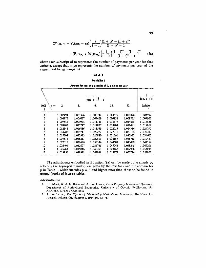
If T, is divided into property tax, PI, and maintenance costs, MI, and the appropriate multiplier is applied to each element, Equation (a), adjusted, becomes :

39

i p[(l + ilk- 11

3. 4. 12. 52.

where each subscript of m represents the number of payments per year for that variable, except that m&) represents the number of payments per year of the annual rent being compared.

TABLE 1

Multiplier

Amount for year of p deposik of i, p times per year

1 lo&U + i>

Infinity

1 2 3 4 5 6 7 8 9

10 11 12

1 .002494 1.004975 1.007445 1.009902 1.012348 1.014782 1.017204 1.019615 1.02201 5 1.024404 1.026783 1 .029150

1.003326 1.006637 1 .009934 1.013217 1.016486 1.019741 1.022983 1.026211 1.029426 1.032627 1.035816 1 .038993

1 .OO3742 1 .007469 1.011181 1.014877 1.018559 1.022227 1.03880 1.029519 1.033144 1 .036755 1.040353 1.043938

1.004575 1 .OO9134 1.013677 1.018204 1.022715 1 .027211 1.031691 1.036157 1.040608 1.045045 1.049467 1.053875

l.oO4896 1.009775 1.014638 1.019485 1.024316 1.029132 1.033932 1.038718 1.043489 1.048245 1.052986 1.057714

1 .OO4992 l.OO9967 1.014926 1.019869 1.024797 1 .029709 1.034605 1.039487 1.044354 1 .049206 1.054044 1 .058867

The adjustments embodied in Equation (8a) can be made quite simply by selecting the appropriate multipliers given by the row for i and the column for p in Table 1, which includes p = 3 and higher rates than those to be found in normal books of interest tables.

REFERENCES 1. J. I. Meek, W. A. McBride and Arthur Lerner, Farm Property Investment Decisions,

Department of Agricultural Economics, University of Guelph, Publication No. AE/1969/1, Page 17, footnote.

2. Arthur Lerner, The Effects of Discounting Methods on Investment Decisions, this Journal, Volume XII, Number 2, 1964, pp. 72-76.