by j. bec , l. biferale , a. s. lanotte arxiv:0904.2314v1 … · 3 isac-cnr, istituto di scienze...

arX

iv:0

904.

2314

v1 [

phys

ics.

flu-

dyn]

15

Apr

200

9

Under consideration for publication in J. Fluid Mech. 1

Turbulent pair dispersion of inertial particles

By J. BEC1, L. B IFERALE2, A. S. LANOTTE3,A. SCAGLIARINI2 and F. TOSCHI4

1 Universite de Nice-Sophia Antipolis, CNRS, Observatoire de la Cote d’Azur,Laboratoire Cassiopee, Bd. de l’Observatoire, 06300 Nice, France

2 Department of Physics and INFN, University of Rome Tor Vergata,Via della Ricerca Scientifica 1, 00133 Roma, Italy

3 ISAC-CNR, Istituto di Scienze dell’Atmosfera e del Clima, Via Fosso del Cavaliere 100,00133 Roma and INFN, Sezione di Lecce, 73100 Lecce Italy

4 Department of Physics and Department of Mathematics and Computer Science, EindhovenUniversity of Technology, 5600 MB Eindhoven, The Netherlands and Istituto per le

Applicazioni del Calcolo CNR, Viale del Policlinico 137, 00161 Roma, Italy

(Received 25 October 2018)

The relative dispersion of pairs of inertial particles in incompressible, homogeneous, andisotropic turbulence is studied by means of direct numerical simulations at two values ofthe Taylor-scale Reynolds number Reλ ∼ 200 and Reλ ∼ 400, corresponding to resolu-tions of 5123 and 20483 grid points, respectively. The evolution of both heavy and lightparticle pairs is analysed at varying the particle Stokes number and the fluid-to-particledensity ratio. For particles much heavier than the fluid, the range of available Stokesnumbers is St ∈ [0.1 : 70], while for light particles the Stokes numbers span the rangeSt ∈ [0.1:3] and the density ratio is varied up to the limit of vanishing particle density.For heavy particles, it is found that turbulent dispersion is schematically governed bytwo temporal regimes. The first is dominated by the presence, at large Stokes numbers,of small-scale caustics in the particle velocity statistics, and it lasts until heavy particlevelocities have relaxed towards the underlying flow velocities. At such large scales, asecond regime starts where heavy particles separate as tracers particles would do. As aconsequence, at increasing inertia, a larger transient stage is observed, and the Richard-son diffusion of simple tracers is recovered only at large times and large scales. Thesefeatures also arise from a statistical closure of the equation of motion for heavy particleseparation that is proposed, and which is supported by the numerical results.In the case of light particles with high density ratios, strong small-scale clustering leadsto a considerable fraction of pairs that do not separate at all, although the mean separa-tion increases with time. This effect strongly alters the shape of the probability densityfunction of light particle separations.

1. Introduction

Suspensions of dust, droplets, bubbles, and other finite-size particles advected by in-compressible turbulent flows are commonly encountered in many natural phenomena (see,e.g., Csanady 1980, Eaton & Fessler 1994, Falkovich et al.. 2002, Post & Abraham 2002,Shaw 2003, Toschi & Bodenschatz 2009). Understanding their statistical properties isthus of primary importance. From a theoretical point of view, the problem is more com-plicated than in the case of fluid tracers, i.e. point-like particles with the same density as

http://arxiv.org/abs/0904.2314v1

2 J. Bec, L. Biferale, A. S. Lanotte, A. Scagliarini, and F. Toschi

the carrier fluid. Indeed, when the suspended particles have a finite size and a density ra-tio different from that of the fluid, they have inertia and do not follow exactly the flow. Asa consequence, correlations between particle positions and structures of the underlyingflow appear. It is for instance well known that heavy particles are expelled from vorticalstructures, while light particles tend to concentrate in their cores. This results in theformation of strong inhomogeneities in the particle spatial distribution, an effect oftenrefered to as preferential concentration (see Douady et al. 1991, Squires & Eaton 1991,Eaton & Fessler 1994). This phenomenon has gathered much attention, as it is revealedby the amount of recently published theoretical work (Balkovsky et al. 2001, Zaichik et al. 2003,Falkovich & Pumir 2004), and numerical studies (Collins & Keswani 2004, Chun et al. 2005,Bec et al. 2007, Goto & Vassilicos 2008). Progresses in the statistical characterization ofparticle aggregates have been achieved by studying particles evolving in stochastic flowsby Sigurgeirsson & Stuart 2002, Mehlig & Wilkinson 2004, Bec et al. 2005, Olla 2002 andin two-dimensional turbulent flows by Boffetta et al. 2004. Also, single trajectory statis-tics have been addressed both numerically and experimentally for small heavy particles(see, e.g., Bec et al. 2006, Cencini et al. 2006, Gylfason et al. 2006, Gerashchenko et al. 2008,Zaichik & Alipchenkov 2008, Ayyalasomayajula et al. 2008, Volk et al. 2008), and for largeparticles (Qureshi et al. 2007, Xu & Bodenschatz 2008). The reader is refered to Toschi & Bodenschatz 2009for a review.In this paper we are concerned with particle pair dispersion, that is with the statistics,

as a function of time, of the separation distanceR(t) = X1(t)−X2(t) between two inertialparticles, labelled by the subscripts 1 and 2 (see Bec et al. 2008, Fouxon & Horvai 2008,Derevich 2008 for recent studies on that problem). In homogeneous turbulence, it issufficient to consider the statistics of the instantaneous separation of the positions of thetwo particles. These are organised in different families according to the values of theirStokes number St, and of their density mismatch with the fluid, β.For our purposes, the motion of particle pairs, with given (St, β) values and with

initial separations inside a given spherical shell, R = |X1(t0)−X2(t0)| ∈ [R0, R0 + dR0]is followed until particle separation reaches the large scale of the flow. With respect tothe case of simple tracers, the time evolution of the inertial particle pair separation R(t)becomes a function not only of the initial distance R0, and of the Reynolds number ofthe flow, but also of the inertia parameters (St, β).A key question that naturally arises is how to choose the initial spatial and velocity

distributions of inertial pairs. Indeed, it is known that heavy (resp. light) particles tendto concentrate preferentially in hyperbolic (resp. elliptic) regions of the advecting flow,with spatial correlation effects that may extend up to the inertial range of scales, asshown in Bec et al. 2007. Moreover, when inertia is high enough, the particle pair velocitydifference, δRV = |V1(X1(t), t) − V2(X2(t), t)|, may not go smoothly to zero when theparticle separations decreases, a phenomenon connected to the formation of caustics,see Wilkinson & Mehlig 2005, Falkovich & Pumir 2007. In our numerical simulations,particles of different inertia are injected into the flow and let evolve until they reach astationary statistics for both spatial and velocity distributions. Only after this transienttime, pairs of particles with fixed intial separation are selected and then followed in thespatial domain to study relative dispersion.By reason of the previous considerations, the main issue is to understand the role

played by the spatial inhomogeneities of the inertial particle concentration field and bythe presence of caustics on the pair separations, at changing the degree of inertia. Weremark that these two effects can be treated as independent only in the limit of verysmall and very large inertia. In the former case, particles tend to behave like tracers andmove with the underlying fluid velocity: preferential concentration may affect only their

Turbulent pair dispersion of inertial particles 3

separation. In the opposite limit, particles distribute almost homogeneously in the flow:however, due to their ballistic motion, they can reach nearby positions with very differentvelocities (Falkovich et al.. 2002). In any other case of intermediate inertia, both theseeffects are present and may play a role in the statistics of inertial pair separation.It is worth anticipating the two main results of this study:

(i) The separation between heavy particles can be described in terms of two time regimes:a first regime is dominated by inertia effects, and considerable deviations from the tracerscase arise in the inertial relative dispersion; in the second one, the tracers behaviour isrecovered since inertia is weak and appears only in subdominant corrections that vanishas 1/t. The crossover between these two regimes defines a new characteristic spatial andtemporal scale, connected to both the size of caustics and the Stokes number, whichinfluences the particle separation for not too long time-lags and not too large scale.(ii) The strong clustering properties that are typical of light particles may lead to the factthat many pairs do not separate at all: their statistical weight is clear in the separationprobability density function (PDF), which develops a well defined power-law left tail.It would clearly be also interesting to investigate the dependence upon the Reynolds

number of the inertial particle pair separation. Small-scale clustering seems to be poorlydependent on the degree of turbulence of the carrier flow (Collins & Keswani 2004,Bec et al. 2007), while much less is known about the Reynolds number dependence ofthe caustics statistics. Our numerical data do not allow to explore this question in detail,so that we will restrict ourselves to show data associated to the two Reynolds numbersin all cases when differences are not significative.In the case of fluid tracers, the standard observables are the time evolutions of the

mean square separation and of the separation probability density function, for whichwell established predictions exist since the pioneering work of Richardson 1929. We con-trast these observables obtained for tracers with the results for heavy and light inertialparticles.The paper is organised as follows. In §2, we briefly recall the basic equations of motion

and describe the numerical simulations. In §3, we analyse the stationary distribution ofheavy particle velocity differences, conditioned on the particle initial separation, high-lighting both the presence of small-scale caustics and the effects of particle inertia atthose scales corresponding to the inertial range of turbulence. In §4 we study the be-haviour of the mean separation distance of heavy pairs, at changing the Stokes numberSt; we also analyse the influence of the caustics in the initial statistics on the subse-quent pair separation evolution. A mean-field model, which is able to capture the mainnumerical findings, is proposed in the same section. The time evolution of the separationprobability density functions is discussed in §5 and we present the data for light particlesin §6. In §7 we summarise the main findings.

2. Equation of motion and numerical details

We present results from direct numerical simulations of turbulent flows seeded withinertial particles. The flow phase is described by the Navier-Stokes equations for thevelocity field u(x, t)

∂tu+ u · ∇u = −∇p+ ν∇2u+ f , ∇ · u = 0 . (2.1)

The statistically homogeneous and isotropic external forcing f injects energy in the firstlow wave number shells, by keeping constant their spectral content (see Chen et al. 1993).The kinematic viscosity ν is chosen such that the Kolmogorov length scale η ≈ δx, whereδx is the grid spacing: this choice ensures a good resolution of the small-scale velocity


N Reλ η δx ε ν τη tdump δt

Run I 512 185 0.01 0.012 0.9 0.002 0.047 0.004 0.0004Run II 2048 400 0.0026 0.003 0.88 0.00035 0.02 0.00115 0.000115

Table 1. Eulerian parametres for the two runs analysed here: Run I and Run II in the text. Nis the number of grid points in each spatial direction; Reλ is the Taylor-scale Reynolds number;η is the Kolmogorov dissipative scale; δx = L/N is the grid spacing, with L = 2π denoting the

physical size of the numerical domain; τη =p

ν/ε is the Kolmogorov dissipative time scale; ε isthe kinetic energy dissipation; ν is the kinematic viscosity; τdump is the time interval betweentwo successive dumps along particle trajectories; δt is the time step.

dynamics. The numerical domain is cubic and 2π-periodic in the three directions of space.We use a fully dealiased pseudospectral algorithm with 2nd order Adam-Bashforth time-stepping (for details see Bec et al. 2006, Cencini et al. 2006). We performed two series ofDNS: Run I with numerical resolution of 5123 grid points, and the Reynolds number atthe Taylor scale Reλ ≈ 200; Run II with 20483 resolution and Reλ ≈ 400. Details of theruns can be found in Table 1.The particle phase is constituted by millions of heavy and light particles— the latter

only for Run I—with different intrinsic characteristics. Particles are assumed to be withsize much smaller than the Kolmogorov scale of the flow, η, and with a negligible Reynoldsnumber relative to the particle size. In this limit, the equations ruling their dynamicstake the particularly simple form:

X = V , V = −1

τs[V − u(X, t)] + β Dtu(X, t) , (2.2)

where the dots denote time derivatives. The particle position and velocity are (X(t),V (t)),respectively; u(X(t), t) is the Eulerian fluid velocity evaluated at the particle position,and Dtu is the so-called added mass term, which measures the fluid acceleration alongparticle trajectory. The adimensional constant β = 3ρf/(ρf+2ρp) accounts for the addedmass effect through the density contrast between particles ρp and fluid ρf . The parti-cle response time, appearing in the Stokes drag, is τs = 2ρpa

2/(9ρfν), where a is theparticle radius. Particle inertia is quantified by the Stokes number that is defined asSt = τs/τη, where τη = (ν/ε)1/2 is the flow Kolmogorov timescale and ε the averagerate of energy injection. Equation (2.2) has been derived in Maxey & Riley 1983 underthe assumption of very dilute suspensions, where particle-particle interactions (collisions)and hydrodynamic coupling to the flow can be neglected.For Run I, we show results for the following set of (St, β) families: (i) very heavy

particles [β = 0]: St = 0.0, 0.6, 1.0, 3.3; (ii) light particles [β = 2, 3]: St = 0.3, 1.2, 4.1.For each family the typical number of particle pairs that are followed is around 5× 104.For Run II, we show results only for heavy particles but with a larger range of variation inthe Stokes number: St = 0.0, 0.6, 1.0, 3.0, 10, 30, 70. Typical number of particle pairs foreach family is ∼ 104. Once injected particles have relaxed to their steady-state statistics,pairs have been selected with the following initial separations: R0 ≤ η and R0 ∈ [4 : 6]ηfor both Run I and Run II, and R0 ∈ [9 :11]η for Run II only.Beside the time evolution of particle pairs, we also have instantaneous snapshots of

the two phases (fluid and dispersed), with a much higher particle statistics: around 106

per family for Run I, and 108 per family for Run II. These are used to measure thestationary— i.e. not along the trajectories—distribution of particle velocity incrementsdiscussed in next section.


3. Stationary distributions: velocity increments conditioned on

particles separation

Turbulent pair dispersion for tracers is classically based on the application of similaritytheory for Eulerian velocity statistics: depending on the value of space and time scales,velocity increment statistics differently affect the way tracers separate. This results indifferent regimes for relative dispersion, see e.g. Sawford 2001.

In the case of inertial particles, the same reasoning holds, so that to analyse the wayinertial pairs separate in time, the stationary statistics of particles velocity differenceshas to be investigated first. A stationary distribution for the typical velocity differencesbetween two inertial particles is obtained by imposing periodic boundary conditions insidethe physical volume and then measuring velocities on such a thermalised configuration.

We are interested in the scaling behaviour of velocity increments at varying the degreeof inertia and the distance between the particles (in the dissipative or inertial range ofthe turbulent fluid flow). To fix the notation, we denote by U0 the typical large-scalevelocity of the fluid tracers and by L the integral scale of the flow. Moreover we define

δRVSt = |V1(X1(t))− V2(X2(t))|, (3.1)

as the velocity difference at scale R, conditioned on the presence of a pair of particles withStokes number St, separated with a distance R = |X1(t0) −X2(t0)|. Since we are hereinterested in the case of heavy particles only, the Stokes number is sufficient to identifya given particle family. For convenience, we introduce a specific notation for the tracerstationary velocity statistics: δRu = δRV(St=0), which is exactly equal to the Eulerianvelocity increment at scale R.

Recently, Bec et al. 2008 have shown that to describe inertial pair dispersion in syn-thetic flows it is useful to introduce the local or scale-dependent Stokes number, using theratio between the particle response time and the typical eddy turnover time τR = R/δRuof the underlying fluid at a given scale: St(R) = τs/τR ∼ τsδRu/R. For real turbulentflow where different scaling ranges are present, we can equivalently define a scale de-pendent Stokes number St(R) that recovers the usual definition of the Stokes numberSt(R) ≃ St = τs/τη when R ≪ η and behaves as St(R) ∼ τsε

1/3R−2/3 when R ≫ η. Thetypical behaviour of St(R) is sketched in Fig. 1, for two different values of the Stokesnumber St = 3, 70 and using a Batchelor-like parametrisation of the fluid velocity (seeMeneveau 1996):

δRu = U0R

(η2 +R2)1/3. (3.2)

For Stokes numbers, St, order unity or larger, there always exists a typical scale wherethe local Stokes number, St(R), becomes order unity,

R∗(St) = η St3/2. (3.3)

Such a scale, which is well in the inertial range if the Stokes number St is sufficiently large,can be considered a rough estimate of the upper bound for the region of scales where in-ertia plays an important role in the particle dynamics. We expect that two main featuresmight be important in characterising the inertial particle stationary velocity statisticsδRV , with respect to that of tracers δRu. The first concerns the small-scale behaviour ofthe particle velocity statistics. At small scales R ≪ η and for large-enough Stokes num-bers, the presence of caustics makes the particle velocity increments not differentiable.


10-1

100

101

10-2 100 102

St(

R)

R/η

δR*u(St=3)δR*u(St=70)

10-2

10-1

100

101

<|δ

Ru|

>

0

0.2

0.4

0.6

0.8

1

1.2

10-2 10-1 100 101 102

St

γ(St)

Figure 1. Left panels. Bottom figure: behaviour of the scale-dependent Stokes number, St(R)as a function of the scale R normalised with the Kolmogorov scale η, for two Stokes numbersSt = 3, 70 (bottom and top, respectively). The horizontal thick line is for St(R) = 1. Topfigure: the scaling behaviour for the fluid tracer velocity increments versus the scale as givenby (3.2). Notice that the scales R∗ where St(R∗) = 1 fall in the inertial range of the Eulerianfluid velocity. Right panel: the function γ(St) defining the small scales power law behaviour ofcaustics statistics at changing inertia. Notice that for small values of the Stokes number St,γ → 1, i.e. particle velocity is differentiable; at high inertia, γ → 0 indicating the existence ofdiscontinuities in the particle velocity increment statistics.

This feature can be accounted for by saying that

δRVSt ∼ V ηSt

(

R

η

)γ(St)

; R ≪ η, (3.4)

where the V ηSt is a constant prefactor and the function γ(St) gives the typical scaling

of caustic-like velocity increments. Indeed we do expect that at changing the inertia ofthe particles, the statistical weight of caustics might monotonically vary as follows: atsmall St, limSt→0 γ(St) = 1 , i.e. the value for smooth, differentiable Eulerian statisticsof tracers; at large values St → ∞, it should approach the discontinuous limit γ(St) → 0,valid for particles that do not feel underlying fluid fluctuations at all. The right panelof Fig. 1 shows the typical shape of the function γ(St) that is expected to be valid forturbulent flows.The second important feature concerns the particle velocity statistics at scales larger

than the scale R∗(St) previously defined, but smaller than the integral scale of the fluidflow. For any fixed Stokes number and for a large-enough Reynolds number, we expectthat inertia becomes weaker and weaker, by going to larger and larger scales R ≫ R∗(St).In such a case, particle velocity increments are expected to approach the underlying fluidvelocity increments:

δRVSt → V 0St δRu ∼ V 0

St U0

(

R

L

)1/3

; R∗(St) ≪ R ≪ L, (3.5)

where for simplicity we have neglected possible intermittent correction to the Kolmogorov1941 (K41) scaling of the fluid velocity (see Frisch 1995 for details). Clearly, the Reynoldsnumber has to be sufficiently large to provide a well-developed scaling region R∗(St) ≪R ≪ L, before approaching the large scale L. We emphasise that in (3.5), an adimensional


10-4

10-3

10-2

10-1

100

101

10-2 10-1 100 101 102

<|δ

RV

St|>

R/η

R

R1/3

St=0St=0.6

St=1St=10St=70

10-1

100

100 101 102

R/η

0.5

0.8

1

0 20 50 80

V0St

St

Figure 2. Right figure: particle velocity structure function of order p = 1 versus the scale R/η,for various Stokes numbers, St = 0, 0.6, 1, 10, 70, and for Reynolds number Reλ ∼ 400, Run II.The statistics for fluid tracers (St = 0) correspond to the solid line. Statistical errors are of theorder of twice the size of symbols for scales smaller then η and become comparable with the sizeof symbols in the inertial range of fluid velocity statistics. The differentiable scaling behaviour∝ R in the dissipative range, and the Kolmogorov 1941 behaviour ∝ R1/3 in the inertial rangeof scales are also shown. Left figure: zoom-in of the inertial range, same symbols as right. Inset:behaviour of the amplitude prefactor, V 0

St as a function of the Stokes number St, as measuredfrom the velocity increments at the integral scale L, Run II.

normalisation factor V 0St has been introduced: it takes into account possible filtering ef-

fects induced by inertia at large scales. The normalisation is such that V 0(St=0) = 1, while

for any Stokes larger than zero V 0(St) ≤ 1.

In Fig. 2 we test the validity of the previous picture by analyzing the typical velocityfluctuation, 〈|δRVSt|〉, at changing Stokes number and for data of Run II at Reynoldsnumber Reλ ∼ 400. At small scales one detect the presence of caustics in the velocitystatistics, with a non smooth scaling behaviour below the Kolmogorov scale η. At scaleswithin the inertial range and when the Stokes number is sufficiently large, the effect ofcaustics affects also particle velocity statistics, up to a characteristic scale which becomeslarger and larger by increasing particle inertia. Beyond this scale, particle velocity incre-ments tend to approach the scaling behaviour of the fluid tracers, but their amplitudeis depleted of a factor 1/V 0

St, which increases with the Stokes number, as shown in theinset of the right-hand panel of Fig. 2. A similar behaviour is expected for higher orderfluctuations, if we neglect the role of intermittency.It is interesting to consider the scaling behaviour of particle velocity in terms of the

underlying velocity statistics, not only at very small or very large separations, but forany value of the scale R. This is not straigthforward, since we have to account not onlyof the fluid Eulerian statistics at the dissipative and inertial range of scales, but also themodifications due to the inertia. This is responsible, as we have seen, for the appeareanceof a new relevant scale, and for filtering effects in the velocity amplitude.To fully characterise particle velocity increments, we notice that the Stokes scale,

R∗(St) defines a typical Stokes-velocity: this is the fluid velocity increment at the Stokesscale, δu∗(St) ∼ δR∗u (see left panel of Fig. 1). Previous reasonings can be summarisedin the following interpolation formula for the heavy particle velocity increment:

δRVSt = V 0St (δRu)

γ(St(R))[

(δRu)2 + c1 (δu

∗(St))2][1−γ(St(R))]/2

. (3.6)

The above expression is a Batchelor-like parametrisation but in the velocity space, witha transient velocity given by the Stokes velocity, δu∗(St).


10-4

10-3

10-2

10-1

100

101

102

10-2 10-1 100 101 102

<|δ

R V

St|>

R/η

St=0St=0.6

St=1St=10St=70

0

0.5

1

1.5

2

100 101 102

Figure 3. Scaling behaviour of the particle velocity structure function of order one, versus thenormalised scale R/η. Solid lines: fit of the data of Fig. 2, Run II, using the interpolation formula(3.6). Here the large scale prefactors V 0

St are those measured on Run II of the simulation, andshown in the inset of the right panel of Fig. 2. Inset: enlargement of the crossover range, whereδRu ∼ δRV .

Once known the large scale normalization function V 0St, the caustic exponent γ(x)

(introduced in Bec et al. 2005) and the reference fluid velocity increment δRu, then theformula has one free parameter only. It is the prefactor c1 appearing in front of the Stokesvelocity δu∗(St), whose value depends again on the inertia of the particles.In Fig. 3, we show the result of the fit in terms of the expression (3.6), where the caus-

tics scaling exponent has been chosen as γ(x) = [1− 2/π atan(x)]: this functional formprovides a good fit to the numerical results. Details of the small-scale caustic statisticswill be reported elsewhere.The qualitative trend is very well captured by the interpolation function proposed.

Notice that in (3.6), the argument of γ(St) is not the simple Stokes number at theKolmogorov scale, but the scale-dependent one St(R): γ(St) → γ(St(R)). This furtheringredient is needed to take into account the fact that in presence of a rough underlyingfluid velocity, as it happens in the inertial range of scales, no simple power law behaviouris expected for the scaling of particle velocity statistics. This was previously remarked inBec et al. 2008, in the study of heavy particle turbulent dispersion in random flows.Equation (3.6) clearly matches the two limiting behaviours for very small and very large

separations. In the former case, inertia dominates the small-scale velocity statistics withrespect to the underlying smooth fluid velocity, and caustics lead to a pure power-lawbehaviour,

δRV ∼ (δRu)γ(St) ∼ V 0

St

(

R

L

)γ(St)

; R ≪ η, (3.7)

where the local Stokes number has attained its dissipative limit St(R) → St.In the latter case, at very large scales R ≫ R∗(St) inertia is subleading, and the typical

velocity difference between particles is close to the fluid velocity increment,

δRVSt ∼ V 0St δRu; η ≪ R∗(St) ≪ R. (3.8)

At intermediate scales, for large Stokes, St ≥ 1, inertia brings a non-trivial dependencyvia the scale-dependent Stokes number, St(R), and we expect a pseudo power-law scaling:

δRVSt ∼ (δRu)γ(St(R)) ∼ Rγ(St(R))/3; η ≪ R ≪ R∗(St) . (3.9)

Summarising, we propose that at changing the Stokes and Reynolds numbers, different


St

Rδ δ uRSt =

R = (St)R*

ηR

/

1

1 A

B

C

V

Figure 4. Sketch of the different regimes expected in the parameter space of inertia, St, andscale separation R. The curve St(R∗) = 1 separate the region of low inertia St(R) ≤ 1, region(C), from the regions where inertia is important St(R) ≥ 1, regions (A) and (B). Further wecan distinguish the separation regime where inertia is important and particle velocity differencelarger than the fluid one at the same scale, region (A), from the intermediate regime whereinertia is still important particle velocity difference is smaller that the corresponding fluid one,region (B). Separation between region (A) and (B) is given by the curve δRVSt = δRu. Forrelative dispersion of pairs of Stokes St starting at a given separation R, one typically startsfrom the corresponding position in this plane and then evolve upwards along the vertical arrow.

regimes governing the particle velocity statistics can be distinguished. The relevanceof such regimes of the particle velocity statistics for the associate relative dispersiondynamics can be easily explained with the help of the sketch reported in Fig. 4. In theparameter space of inertia and scale separation (St,R), we can distinguish three regionsdepending whether inertia is strong or weak, and whether particle velocity difference islarge or not with respect of the fluid velocity difference at comparable scale. In agreementwith what commented before, we pose that the curve St(R∗) = 1 distinguishes the regionof weak (St(R) ≤ 1) and strong inertia (St(R) ≥ 1).Regime (A) is such that inertia is important since the scale R∗(St) ≫ η, and moreover

the typical particle velocity increments are larger than the fluid increments. In the region(B), inertia is still important but particle velocity increments are depleted with respect tothe fluid increments. This typically happens for large Stokes numbers, and in our DNS isvisible only for very large separations R(t) of the highest Stokes St = 70. Finally, regime(C) is characterised by a weak inertia, which appears only in the filtering factor forthe velocity large-scale amplitude and possibly in sub-leading corrections to the tracersrelative dispersion.Even for the largest value of the Reynolds and Stokes numbers achieved in our DNS, it

is very difficult to disentangle quantitatively the above mentioned regimes, because of thecloseness of the three relevant scales, η, R∗(St), and L. Still, the quality of the fit shownin Fig. 3 using the global functional dependence given by Eqn. (3.6) makes us confidentthat the main physical features are correctly captured. Before closing this section, wenote that there is no reason to assume that the functional form entering in the pseudo-power law scaling in the inertial range, γ(St(R)), in (3.9) is equal the one characterizingthe scaling in the viscous range, γ(St), in Eqn. (3.7). Hint for this observation comefrom results obtained in Bec et al. 2008 for random flows, where a very high statisticalaccuracy can be achieved: there, depending if the underlying fluid velocity is spatiallysmooth or rough, a slightly different functional form has been found.The previous analysis gives us a clear quantitative picture of the scale and velocity

ranges where caustics play a role in the particle dynamics. For example, for moderate


Stokes numbers, we have important departure from the tracers statistics only for verysmall scales, i.e. caustics gives a singular contributions to the particle velocity incrementsinside the viscous range; then, at larger scales, the particle velocity scaling become indis-tinguishable from the tracer velocities. Clearly, for such Stokes, no important correctionsfor particle separation evolution is expected with respect to the usual Richardson disper-sion observed for tracers. This is because particle pairs tends to separate, and very soonall pairs will attain separations where their velocities are very close to the underlyingfluid. On the other hand, for very heavy particles, those with Stokes time falling insidethe inertial range of fluid velocity statistics, the contribution from the caustics will be feltalso at relatively large scales, up to R ∼ R∗(St). Pair separations attain such scales whenthe initially large relative velocity difference has relaxed and become smaller than thecorresponding fluid one—crossing from region (A) to (B). Notice that at R ∼ R∗(St),we have that δR∗VSt ≃ V 0

StδR∗u, i.e. there is a non-trivial effect from inertia. Moreover,for large Stokes, at scales R > R∗(St), particle velocity increments are smaller than thefluid counterparts, indicating an important depletion induced by the Stokes drag on theparticle evolution.It is clear from the above discussion that new physics should appear for the value of in-ertia and scales separation of region (B). This regime—that we can not access with thepresent data— is the one where a new law of pair separation should appear as recentlysuggested by Fouxon & Horvai 2008. A discussion of the dispersion regimes of inertialparticle pairs follows in the next section in terms of the time behaviour of the meansquare separation distance.

4. Dispersion regimes and corrections due to inertia

In this section we analyse the effects of inertia on the mean square separation of heavyparticle pairs with a given initial separation distance, R0 at time t = t0, as a function ofthe Stokes number:

〈(R(t))2 |R0, t0〉St = 〈|X1(t)−X2(t)|2〉St, (4.1)

where in the left-hand side the average is performed over all pairs of particles such that|X1(t0) − X2(t0)| = R0. The study of the relative dispersion of small, neutrally buoy-ant tracer particles has recently been the subject of renewed interest. This has beenmotivated by the fact that very accurate—highly resolved in time and space—datahave become available, experimentally (Ott & Mann 2000, Bourgoin et al. 2006) and nu-merically (Yeung & Borgas 2004, Biferale et al. 2005, Biferale et al. 2006). These studieshave confirmed what was known since the works of Richardson 1929 and Batchelor 1952,i.e. the existence of different dispersive regimes for tracer pairs in turbulent flows, de-pending on the value of their initial distance and on the time scale considered.When released in a statistically homogeneous and isotropic, turbulent flow with an

initial separation R0 in the inertial range for fluid velocity, i.e. η ≃ R0 ≪ L, tracer pairsinitially separate according so the so-called Batchelor regime,

〈(R(t))2|R0, t0〉St=0 ≃ R20 + C(εR0)

2/3 t2; τη ≪ (t− t0) ≪ tB , (4.2)

where C is supposed to be a universal constant, and ε is the average kinetic energydissipation of the flow. This ballistic regime appears because initially tracers separate asif the underlying velocity field were frozen, and it lasts for a time scale that is a function

of the initial separation itself, tB =(

R20/ε

)1/3(see Batchelor 1952, Bourgoin et al. 2006).

After such a transient initial time, the relative separation dynamics forgets the initial


100

101

102

103

104

105

106

10-1 100 101 102

<(R

(t))

2 >/η

2

t/τη

R(t0) ε [ 0 : 1 ] η

St=0St=0.6

St=1St=3.3

1

10

10-1 100 101

Q(t)

100

101

102

103

104

105

106

10-1 100 101 102

<(R

(t))

2 >/η

2

t/τη

R(t0) ε [ 4 : 6 ] η

St=0St=0.6

St=1St=3.3

1

2

10-1 100 101

Q(t)

Figure 5. Mean square separation versus time, for heavy particles at changing St and the initialdistance R0. Time is normalised with the Kolmogorov time scale τη. Left panel: St = 0, 0.6, 1,and 3.3; initial distance R0 ∈ [0 : 1]η, Run I. Error bars due to statistical fluctuations are of theorder of the symbol size. Notice that the two largest Stokes numbers show a time lag intervalwhere separation proceeds faster than tracers. Inset: ratio between the heavy particle separationand the tracer data, Q(t) versus time, for St = 0.6, 1, and 3.3. Same symbols as in the body ofthe figure are used. Right panel: mean square separation versus time, but with a larger initialdistance, R0 ∈ [4 : 6]η. Stokes numbers are the same as in the left panel. Notice that now onlythe dispersion of particle pairs with St = 3.3 exhibits a small departure from the underlyingfluid, as shown by the Q(t) indicator in the inset. For the smaller Stokes, typical size of causticsis smaller than the initial separation R0, and particle pairs therefore separate as fluid tracersdo.

conditions and tracers separate explosively with a power law behaviour given by theRichardson law:

〈(R(t))2|R0, t0〉(St=0) ∼ g t3; tB ≪ (t− t0) ≪ TL , (4.3)

where g is known as the Richardson constant. As set out in Monin & YaglomMonin & Yaglom 2007,the tracer separation PDF—that will be discussed later—has a similar scaling behaviourin these ranges.A remarkable fact of the Richardson dispersion (4.3) is the disappearance of the

dependence on the initial separation R0, an effect also dubbed intrinsic stochasticity

(E & Vanden Eijnden 2000), which is just the signature of the non-Lipschitz nature ofthe velocity field driving the separation between tracers, when their mutual distance is inthe inertial range of fluid velocity statistics. The experimental and numerical validationof the previous prediction (4.3) has proved to be particularly difficult, the main reasonbeing the strong contamination from viscous and large scale effects in the tracers dynam-ics. To overcome these problems, a series of techniques have been developed, includingthe study of doubling time statistics; i.e. the probability distribution function of the timeneeded for a pair to double its separation (Boffetta & Sokolov 2002, Biferale et al. 2005).Thanks to these techniques, a fairly good agreement on the value of the Richardson con-stant has been achieved. Here, we want to study how the tracer behaviour is modified bythe presence of small-scale caustics in particular and by inertia effects in general, for thecase of heavy particle pairs. Standard direct measurements of the moments of separationas a function of time will be considered, while application of doubling time statistics isleft for future studies.In Fig. 5, we show the behaviour for the mean square separation at varying the Stokes

number, and for two values of the initial separation. We start with data at the lowestresolution, i.e. Run I at Reλ ≃ 200, and for moderate Stokes numbers, St ∼ O(1). Initialdistances are chosen equal to R0 ≤ η (left panel) and R0 ∈ [4 :6] η (right panel).If the initial distance is small enough (left panel), the presence of caustics in the particle


10-1

100

101

102

103

104

105

106

107

10-1 100 101 102

<(R

(t))

2 >/η

2

t/τη

R(t0) ε [ 0 : 1 ] η

t2

t3

St=0St=10St=30St=70

101

102

103

104

105

106

107

10-1 100 101 102

<(R

(t))

2 >/η

2

t/τη

R(t0) ε [ 4 : 6 ] η

t2

t3

St=0St=10St=30St=70

Figure 6. Mean square separations versus time, for pairs with St = 10, 30, 70, at Reλ = 400.Left and right panels refer to the two initial distance R0 ∈ [0 :1]η and R0 ∈ [4 :6]η, respectively.Error bars due to statistical fluctuations are of the order of the symbols size. Tracers (solid lines)are also shown for comparison. Notice the ballistic behaviour for the heavy particle separationobserved in the caustics dominated time interval. For very large time-lags a Richardson-likebehaviour starts to develop but with a less intense overall speed of separation, due to the

depletion effects of the V(0)St prefactor in the particle velocity increments for large Stokes numbers.

The slopes of the Batchelor, 〈R2(t)〉 ∝ t2, and Richardson, 〈R2(t)〉 ∝ t3 dispersion regimes arealso drawn for reference.

velocity field at initial time gives a very remarkable departure from the tracer behaviour.At increasing the Stokes number, such departure is more and more evident, and it lastsfor a time lag which becomes longer and longer. For the highest value of the Stokesnumber shown in the left panel of Fig. 5 (St = 3.3), a sensible difference from the tracerbehaviour is observed over almost two decades: t ∈ [0.1:10] τη. A way to better visualisethe departure from the tracer statistics consists in plotting the mean square separationfor heavy pairs of different Stokes numbers, normalised to the tracer one, that is

Q(t) =〈(R(t))2〉St

〈(R(t))2〉(St=0). (4.4)

This quantity is shown in the insets of Figure 5. For heavy pairs starting at R0 ≃ η andwith St = 3.3, the relative difference is as large as 10 at its maximum for t ∼ τη. However,such effect becomes progressively less important if we start the separation experimentfrom larger initial distances as shown in the right panel of the same figure. This is because,at these same Stokes numbers, the deviation of particle velocity difference with respectto the underlying fluid, due to caustics, has already decreased. This is equivalent to statethat, for these Stokes numbers, the typical size of caustics is smaller than the initialseparation R0, and particle pairs therefore separate as fluid tracers do. At larger timelags, whatever the value of the initial separation, the Richardson dispersion regime isrecovered.We now consider what happens for larger Stokes numbers. In Fig. 6, we show the resultsfor the mean square separation of St = 10, 30, and 70 and for the large Reynolds number,Reλ ≃ 400. Both initial distances, R0 ∈ [0 : 1]η and R0 ∈ [4 : 6]η are displayed. As onecan see, for the large value of St = 70, the tracer-like behaviour is never recovered,and even the separation of pairs starting with the largest distance R0 is affected. Thetransient regime dominated by the caustics invades the whole inertial range: since particlepairs need a very long time to decrease their initial velocity difference to the valueof the fluid increment at the corresponding scale, they separate with a quasi-ballisticbehaviour:〈R2(t)〉St ∝ t2.The above scenario can be interpreted in terms of caustic-dimensions. At any value of the


inertia, there exist a spatial length, of the order of the scale R∗(St), which identifies thetypical spatial size of caustics, i.e. the range of scales where particle velocity incrementsare uncorrelated from the underlying fluid velocity field. If the initial pair separationR0 is taken inside this region (left panel of Fig. 5), particle pair separation starts muchfaster than for fluid tracers, because of the much more intense velocity differences felt bythe pairs inside the caustics. When particle pairs reach a separation larger than R∗(t),they start to be synchronised with the underlying fluid velocity, recovering the typicalRichardson dispersion. However, if the initial separation is larger than the caustics size,the evolution of inertial particle pairs is almost indistinguishable from the tracers. Finally,whether or not a Richardson-like behaviour is recovered for very large inertia, may dependon the Reynolds number also. In the limit of larger and larger Reynolds, at fixed Stokesnumber, one may expect a final recovery of the fluid tracers behaviour even for veryheavy particle pairs.

4.1. Mean-field approach to heavy particle dispersion

The turbulent relative dispersion of fluid tracers can be easily modelled by applying K41scaling theory to the fluid velocity increments governing particle separation dynamics(see, e.g., Ouellette et al. 2006). Indeed, if R(t) is the tracer separation vector at a giventime, its evolution is completely specified by the equation

R(t) = u(X1, t)− u(X2, t) = δRu(R, t) , (4.5)

together with the initial condition R(t0) = R0. Hence, we can directly write an equationfor the root-mean-square separation r(t) ≡ 〈|R(t)|2 |R0, t0〉

1/2

r =1

r〈R(t) · δRu(R(t), t) |R0, t0〉 , with r(t0) = R0. (4.6)

We next assume the following mean-field closure for the right-hand side:

〈R(t) · δRu(R(t), t) |R0, t0〉 ≈ 〈R2 |R0, t0〉1/2 〈R · δRu〉 = r S//

1 (r), (4.7)

where S//

1 (r) is the first-order Eulerian longitudinal structure function of the underly-ing homogeneous and isotropic turbulent flow. According to K41 phenomenology, thisstructure function behaves in the inertial range as S//

1 (r) ≃ C ε1/3r1/3, where C is anorder-unity constant. This closure finally leads to

r = C ε1/3r1/3, so that r(t) =[

R2/30 + (2C/3) ε1/3(t− t0)

]3/2

. (4.8)

Such an approximation gives a complete qualitative picture of the time evolution of themean square separation between tracers. In particular, it encompasses the two important

regimes of relative dispersion: when (t−t0) ≪ tB = (3/2C) ε−1/3R2/30 , a Taylor expansion

of the solution (4.8) gives the Batchelor regime r(t) ≃ R0 + C (εR0)1/3 (t − t0), while

when (t− t0) ≫ tB , one recovers Richardson’s law r(t) ≃ (2C/3)3/2ε1/2 t3/2.In the case of inertial particles, the number of degrees of freedom to describe the

dynamics is obviously increased: the separation between two heavy particles obeys

R(t) = −1

τs

[

R(t)− δRu(R, t)]

. (4.9)

In order to derive mean-field equations one has to track simultaneously the average dis-tance and velocity difference between particles. For this we follow the same spirit as fortracers and introduce the particle velocity structure function v(t) ≡ 〈|δRV (t)|2 |R0, t0〉

1/2,where δRV (t) = R(t) is the velocity difference between the two particles. One can pro-


ceed as previously to write from (4.9) exact equations for r(t) and v(t):

r =1

r(v2 − r2)−

1

τs

[

r −1

r〈R · δRu〉

]

, (4.10)

v = −1

τs

[

v −1

v〈δRV · δRu〉

]

, (4.11)

where for the sake of a lighter notation the indication of conditional ensemble averageswas dropped. It is worth noticing that the root-mean-square velocity difference v(t)evolves with a dynamics that resembles closely that of heavy particles. However, v(t)does not coincide with the time derivative of the mean distance r(t). It is thus useful torewrite the above equations introducing a sort of transverse particle velocity componentw defined as

r = v − w . (4.12)

We can write an exact equation also for the evolution of w

w = −1

τsw − (2v − w)

w

r−

1

τs

[

1

r〈R · δRu〉 −

1

v〈δRV · δRu〉

]

. (4.13)

Of course, equations (4.11), (4.12), and (4.13) are not closed without supplying thecorrelation between the particle evolution and the underlying fluid. As in the case oftracers, the first unclosed term appearing in the right-hand side of (4.13) is approximatedby (4.7). The next unclosed term involving the correlation between fluid and particlevelocity differences is approximated by

〈δRV · δRu〉 ≈ 〈|δRV |2〉1/2 〈|δRu|2〉1/2 = v S

1/22 (r) , (4.14)

where S2(r) denotes the full second-order structure function of the fluid velocity field.When r is in the inertial range, K41 phenomenology implies that S2(r) ∝ (εr)2/3. Finallythese approximations lead to a closed set of equations for the time evolution of the averageseparation and velocities r, v, and w

r = v − w , (4.15)

v =1

τs[C ε1/3r1/3 − v] , (4.16)

w = −1

τsw − (2v − w)

w

r+

1

τsB ε1/3r1/3 , (4.17)

where B and C are positive order-unity dimensionless constants, reflecting the lack ofcontrol on the prefactors of the scaling laws in the closures (4.7) and (4.14). This systemof equations is supplemented by the initial conditions r(t0) = R0, v(t0) = 〈|δR0V |2〉1/2

and w(t0) = v(t0)− 〈R0 · δR0V 〉/R0, which clearly depend on the dispersion experimentunder consideration. It is worth noticing that this system of equations reduces to themean-field equation (4.8) for tracers in the limit of vanishing inertia τs → 0.Similarly to the case of tracers, the crude approximation (4.15)-(4.17) of the evolution

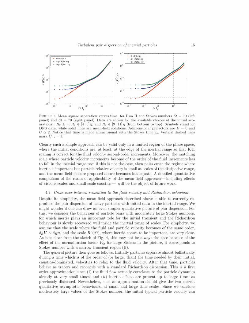
of the root-mean-square distance between heavy inertial particles is able to capture themain features of the separation time behaviour. In Fig. 7, we show the result of thenumerical integration of the set of equation (4.15)-(4.17) obtained by an appropriatechoice of the free parameters (see figure caption), together with DNS data from Run II,for two different large values of the Stokes number. For fixed initial separation and atincreasing the intensity of the caustics velocity increments in the initial condition (i.e. atincreasing inertia), the transient deviation from the Richardson behaviour become moreand more evident at intermediate times (of the order of the Stokes time τs, not shown).


10−2

10−1

100

101

10−6

10−4

10−2

100

102

t / τs

< R

2 (t)

>

0 <R(0)< η4η <R(0)< 6η9η <R(0)< 11η

10−3

10−2

10−1

100

10−6

10−4

10−2

100

102

t / τs

< R

2 (t)

>

0 <R(0)< η4η <R(0)< 6η9η <R(0)< 11η

Figure 7. Mean square separation versus time, for Run II and Stokes numbers St = 10 (leftpanel) and St = 70 (right panel). Data are shown for the available choices of the initial sep-arations : R0 ≤ η, R0 ∈ [4 : 6] η, and R0 ∈ [9 : 11] η (from bottom to top). Symbols stand forDNS data, while solid lines are mean-field solutions. Adimensional prefactors are B = 0 andC ≃ 2. Notice that time is made adimensional with the Stokes time τs. Vertical dashed linesmark t/τs = 1.

Clearly such a simple approach can be valid only in a limited region of the phase space,where the initial conditions are, at least, at the edge of the inertial range so that K41scaling is correct for the fluid velocity second-order increments. Moreover, the matchingscale where particle velocity increments become of the order of the fluid increments hasto fall in the inertial range too: if this is not the case, then pairs enter the regime whereinertia is important but particle relative velocity is small at scales of the dissipative range,and the mean-field closure proposed above becomes inadequate. A detailed quantitativecomparison of the realm of applicability of the mean-field approach— including effectsof viscous scales and small-scale caustics— will be the object of future work.

4.2. Cross-over between relaxation to the fluid velocity and Richardson behaviour

Despite its simplicity, the mean-field approach described above is able to correctly re-produce the pair dispersion of heavy particles with initial data in the inertial range. Wemight wonder if one can draw an even simpler qualitative picture of pair dispersion. Forthis, we consider the behaviour of particle pairs with moderately large Stokes numbers,for which inertia plays an important role for the initial transient and the Richardsonbehaviour is slowly recovered well inside the inertial range of scales. For simplicity, weassume that the scale where the fluid and particle velocity becomes of the same order,δRV ∼ δRu, and the scale R∗(St), where inertia ceases to be important, are very close.As it is clear from the sketch of Fig. 4, this may not be always the case because of theeffect of the normalisation factor V 0

St for large Stokes: in the picture, it corresponds toStokes number with a narrow transient region (B).The general picture then goes as follows. Initially particles separate almost ballistically

during a time which is of the order of (or larger than) the time needed by their initial,caustics-dominated, velocities to relax to the fluid velocity. After that time, particlesbehave as tracers and reconcile with a standard Richardson dispersion. This is a firstorder approximation since (i) the fluid flow actually correlates to the particle dynamicsalready at very small times, and (ii) inertia effects are present up to large times aspreviously discussed. Nevertheless, such an approximation should give the two correctqualitative asymptotic behaviours, at small and large time scales. Since we considermoderately large values of the Stokes number, the initial typical particle velocity can


10−3

10−2

10−1

100

101

102

10−6

10−4

10−2

100

t / τs

< R

2 (t)

>

St = 3

St = 10

St = 70

Figure 8. Mean square separation versus time from DNS data of Run II, for three differentvalues of the Stokes numbers. Notice that time is normalised with the Stokes time τs. Solidlines represent the initial, almost ballistic evolution due to the exponential relaxation of velocitystatistics, and the dashed lines correspond to the Richardson regime. With a suitable tuningof the free parameters, here the Richardson constant g and the initial velocity increment value〈(δRV (t0))

2〉, both temporal behaviours are reproduced.

be assumed to be much larger than the fluid velocity, i.e. |δRV | ≫ |δRu|. Under thesehypotheses, there is an initial time interval during which difference between particlevelocities obeys δRV ≈ −(δRV )/τs [see (4.11)], and thus δRV (t) ≃ (δRV (t0)) e

−(t−t0)/τs .As a consequence, the mean square separation between particles evolves initially as:

〈|R2(t)| |R0, t0〉 = R20 + 2τs〈R(t0) · δRV (t0)〉(1 − e−(t−t0)/τs)

+ τ2s 〈(δRV (t0))2〉(1− e−(t−t0)/τs)2. (4.18)

This should be approximately valid up to a time scale, in the inertial range, where|δRV | ∼ |δRu| ∼ (εR)1/3: it is easy to show that such a time scale is proportional to theparticle response time τs. For larger times, inertia effects become subdominant and heavypair dispersion suddenly gets synchronised to a Richardson like regime. Nevertheless, thisRichardson regime has started only after the previous relaxation has ended, that is at adistance much larger than the original separationR0 of the particle pair. The combinationof this initial exponential relaxation of heavy particles with moderately large inertia, plusthe later standard Richardson diffusion are the two main features due to inertia in theinertial pair dispersion. This is indeed confirmed by Figure (8), where we compare DNSdata for mean square separation, with the two phenomenological regimes just described,for which we have assumed that 〈R · δRV (t0)〉 ≃ 0. As we can see, the main qualitativetrends of the small and large time behaviours are very well captured.

4.3. Subleading terms in the Richardson regime

We have seen in previous subsections that the most noticeable effect of inertia on themean pair dispersion is a long transient regime that takes place before reaching a Richard-son explosive separation (4.3), and that this regime is due to the relaxation of particlevelocities to those of the fluid. As we now argue, at larger times—corresponding toregime (C)—there is still an effect of particle inertia that can be measured in termsof subleading corrections to the Richardson law. To estimate these corrections, let usassume that in the mean-field equation (4.16), the term stemming from the fluid velocityCε1/3r1/3 is much larger than the inertia term τsv. This is true when St(r) ≪ 1, i.e. attimes t when r(t) ≫ R∗(St). In this asymptotic, one can infer that the transverse velocitycomponent w is much smaller than the total velocity v, so that r ≃ v (see eq. (4.12)). In


101

102

10−1

100

t / τs

Q(T

) −

Q(t

)

slope = −1

St = 0.16St = 0.27St = 0.37St = 0.48

Figure 9. Large-time behaviour of the mean square separation normalised to that of tracers asdefined from Eqn. (4.4) for Run I and various values of the Stokes number as labeled. Deviationsfrom the fluid tracer Richardson law behave as (t/τs)

−1. The limiting valueQ(T ) has been chosendifferent from unity as effects of inertia are still present at the largest scale of the flow.

the spirit of the weak inertia expansion derived in Maxey 1987, we next write a Taylorexpansion of (4.16) to obtain

r ≈ v ≈ Cε1/3r1/3 − τs〈|(d/dt) δru|2〉1/2 ≈ Cε1/3r1/3 − τs〈|δra|

2〉1/2, (4.19)

where δra = δr(∂tu + u · ∇u) denotes the increment of the fluid acceleration over theseparation r. Next we assume scaling invariance of the turbulent acceleration field, thatis, according to dimensional arguments of K41 theory, |δra| ∼ ε2/3r−1/3. Equation (4.19)can then be rewritten as

r = Cε1/3r1/3(

1−Aτs ε1/3r−2/3

)

= Cε1/3r1/3 (1−ASt(r)) , (4.20)

where A is an order-unity constant. The initial condition is given by r(t0) = r0 wherethe initial separation has to be chosen such such that St(r0) ≪ 1. We can next integratethe approximate dynamics perturbatively in terms of the small parameter St(r0) byexpanding the separation as r(t) = ρ0(t)+ρ1(t)+ρ2(t)+ . . . . The leading order is ρ0(t) =

[r2/30 +(2C/3) ε1/3t]3/2 and corresponds to the relative dispersion of a pair of tracers. The

first-order correction reads ρ1(t) = −τs ε1/3A ln(ρ0(t)/r0) ρ

1/30 (t). At times much larger

than the Batchelor time associated to the initial separation r0, i.e. for t ≫ ε−1/3r2/30 , the

leading term follows the Richardson explosive law ρ0(t) ≃ (2C/3)3/2ε1/2t3/2. This finally

implies that in the asymptotics t ≫ ε−1/3r2/30 ≫ τs, one can write

r2(t) ∝ g t3[

1−D (t/τs)−1 ln (t/τs)

]

, (4.21)

where g is the Richardson constant introduced in §4 and D is an order-unity factor,which a priori does not depend neither on the particle Stokes number, nor on the initialparticles separation.This behaviour is confirmed numerically as can be seen from Fig. 9 that gives the

behaviours at large times of the ratio Q(t) between the mean square separation of heavyparticles and that of tracers as defined by (4.4). One can clearly see that data almostcollapse on a line ∝ 1/t confirming the behaviour (4.21) predicted above. Only resultsfrom Run I are displayed here. The reason is that the very large time statistics of tracerdispersion in Run II is not as well statistically converged, leading to more noisy data.The qualitative picture is however very similar.To conclude this section, let us stress that we have assumed above K41 scaling to hold


for the acceleration field (and thus for the pressure gradient). However it is well knownthat the scaling properties of pressure are still unclear: they might depend on the turbu-lent flow Reynolds number and/or on the type of flow (see, e.g., Gotoh & Fukayama 2001,Xu et al. 2007). As stated in Bec et al. 2007, rather than being dominated by K41 scal-ing, numerically estimated pressure increments of Run I (Reλ ≃ 200) seem to be ruled bysweeping, so that |δra| ∼ urms ε

1/3r−2/3. One can easily check that this difference in scal-ing leads to a behaviour similar to (4.21), except that this time logarithmic correctionsare absent, and that the non-dimensional constant D depends on the Reynolds numberof the flow. The present numerical data do not allow to distinguish between these twopossible behaviors.

5. Probability density function of inertial particle separation

We now discuss the shape of the probability density function for both light and heavyinertial particles. We focus on the time and scale behaviour of the non-stationary PDF

PSt,β(R, t|R0, t0) , (5.1)

defined as the probability to find a pair of inertial particles (St, β), with separation R attime t, given their initial separation R0 at time t0. The case of tracers (St = 0, β = 1)has been widely studied in the past, either experimentally, numerically and theoreti-cally for two and three dimensional turbulent flows (see Richardson 1929, Batchelor 1952,Jullien et al. 1999, Boffetta & Sokolov 2002, Biferale et al. 2005, Bourgoin et al. 2006, Salazar & Collins 2009).Following the celebrated ideas of Richardson, phenomenological modelling in terms of adiffusion equation for the PDF of pair separation leads to the well-known non-Gaussiandistribution,

PSt=0,β=1(R, t) ∝R2

(

ε1/3t)9/2

exp

[

−AR2/3

ε1/3 t

]

, (5.2)

which is valid for times within the inertial range τη ≪ t ≪ TL, and is obtained assuminga small enough initial separation and statistical homogeneity and isotropy of the three-dimensional turbulent flow. Here, A is a normalization constant. This prediction is basedon the simple assumption that, for inertial range distances, tracers undergo a diffusiondynamics with an effective, self-similar, turbulent diffusivity K(R) ∝ R δRu ∼ ε1/3 R4/3.Moreover, it relies on the phenomenological assumption that tracers separate in a short-time correlated velocity field. Indeed, it is only if the latter is true, that the diffusionequation for the pair separation becomes exact (see Falkovich et al. 2001).As mentioned before such a scenario may be strongly contaminated by particle inertia.

The main modifications are expected to be due to the presence of small-scale causticsfor small-to-large Stokes numbers, and to preferential concentration. Caustics make thesmall scale velocity field not differentiable and not self-similar, as if inertial particleswere separating in a rough velocity field whose exponent were depending on distance.Preferential concentration, leading to inhomogeneous spatial distribution of particles,manifests itself as a sort of effective compressibility in the particle velocity field.There exists a series of stochastic toy models for Lagrangian motion of particles in

incompressible/compressible velocity fields, where the statistics of pair separation canbe addressed analytically. Among these, the so-called Kraichnan ensemble models, wheretracer particles move in a compressible, short-time correlated, homogeneous and isotropicvelocity field, with Gaussian spatial correlations (we refer the reader to the reviewFalkovich et al. 2001 for a description of this model). It is useful for the sequel to re-call two main results obtained for relative dispersion in a Kraichnan compressible flow.


We denote with ℘ the velocity field compressibility degree†, and with 0 ≤ ξ < 2 the scal-ing exponent of the two-point velocity correlation function at the scale r, in d-dimensions:〈[ui(r)− ui(0)][uj(r)− uj(0)]〉 ∼ G1r

ξ[(d− 1+ ξ−℘ξ)δij + ξ(℘d− 1)rirj/r2]. For parti-

cles moving in such flows, it is possible to show that the pair separation PDF for tracerparticles follows a Richardson-like behaviour:

Pµ,ξ(R, t) ∝RD2−1

t(d−µ)/(2−ξ)exp

[

−AR2−ξ

t

]

. (5.3)

Here µ = ℘ξ(d+ ξ)/(1+℘ξ) and D2 = d−µ is the correlation dimension, characterizingthe fractal spatial distribution of particles.A different distribution emerges when the d−dimensional Kraichan flow is differentiable,i.e. for ξ = 2; in such case, a log-normal PDF is expected:

Pµ,ξ(R, t|R0, t0) ∝1

Rexp

[

−(log(R/R0)− λ(t− t0))

2

2∆(t− t0)

]

, (5.4)

with ∆ = 2G1(d − 1)(1 + 2℘) and λ = G1(d − 1)(d − 4℘). It is worth noticing that inthe latter case, since the flow is differentiable, the large-time PDF depends on the initialdata.

The problem of inertial particle separation in a real turbulent flow presents somesimilarities with the previous toy cases but also important differences.First, the effective degree of compressibility—due to preferential concentration of inertialparticles— , is properly defined only in the dissipative range of scales. For r ≪ η, it isequal to the correlation dimension D2 defined as p(r) ∼ rD2 , where p(r) is the probabilityto find two particles at distance smaller than r, with r ≪ η. As it has been numericallyshown in Bec et al. 2007, Calzavarini et al. 2008 for three-dimensional turbulent flows,the correlation dimension depends only on the degree of inertia (St, β), while it does notseem to depend on the Reynolds number of the flow. For r ≫ η, the effective degree ofcompressibility is no longer constant, but varies with the scale.Second, the underlying velocity field exhibits spatial and temporal correlations that aremuch more complex than in a Gaussian short-correlated field. Such correlations lead tonon-trivial overlaps between particle dynamics and the carrying flow topology. As a result,it is not possible to simply translate the analytical findings obtained in the compressibleKraichnan ensemble to the case of inertial particles: we may expect however that in somelimits the compressible Kraichnan results should give the leading behaviour also for thecase studied here of inertial particles in real turbulent flows.

With this purpose, we first notice that the separation probability density functionthat is valid in the rough case (5.3) has an asymptotic stretched-exponential decay thatis independent on the compressibility degree. This suggests that inertial particle PDF(5.1) must recover the Richardson behaviour (5.2) of tracers in the limit of large scalesand large times. Coherently with what discussed in previous sections, for large times andfor scales larger than R∗

St, we expect that the heavy pairs (in the limit β ∼ 0) PDFrecovers a tracer like distribution :

PSt,0(R, t) ∼ exp

[

−AR2/3

ε1/3t

]

; R ≫ R∗

St. (5.5)

For pairs of light particles, there is no straightforward formulation of such a prediction:

† The compressibility degree ℘ is defined as the ratio ℘ ≡ C2/S2, where C2 ∝ 〈(∇ · u)2〉 andS2 ∝ 〈(∇u)2〉, and varies between ℘ = 0 for incompressible flows, and ℘ = 1 for potential flows.


10-4

10-3

10-2

10-1

100

101

10-1 100 101 102

R/η

St=0

t

t=0

10-1 100 101 102

R/η

St=0.6

t

t=0

10-4

10-3

10-2

10-1

100

101

10-1 100 101 102

R/η

St=3.3

t

t=0

10-1 100 101 102

R/η

St=70

t

t=0

Figure 10. Separation probability density function, P(R, t|R0, t0), for heavy pairs with differentStokes numbers, at changing time. Initial distance is taken R0 ∈ [3 : 4] η for St = 0 (top-left),St = 0.6 (top-right), and St = 3.3 (bottom-left) of Run I, and equal to R0 ∈ [4 :6] η for St = 70(bottom-right) of Run II. The related initial distributions are pictorically depicted with a greyarea. Times shown are: (t − t0)/τη = 1, 6, 18, 36 for Run I and (t − t0)/τη = 1, 6, 18, 36, 86 forRun II.

as we shall see in the sequel, preferential concentration effects have a strong fingerprinton the separation PDF even at large times and large scales.

In the opposite limit of very small separations, i.e. R ≪ η, one can correctly assumethat the effective degree of compressibility is constant and therefore apply either thesmall-scale limit for rough flows (5.3), or that for smooth flows (5.4), depending on thescaling properties of the particle velocity field entailed in the value of the exponent γ(St),defined from (3.4) and related to the caustics. We thus expect

PSt,β(R, t|R0, t0) ∼ RD22 −1G(t), if γ(St) 6= 1,

PSt,β(R, t|R0, t0) ∼ RD2−1F (t), if γ(St) = 1. (5.6)

Here F and G are two different decaying functions of time t, whose expression can beeasily derived from (5.3)-(5.4). Notice that for the smooth case, i.e. the small-scale limit ofthe log-normal distribution (5.4), we get for the spatial dependency a factor D2/2 insteadof the factorD2 of the rough case. This will matter in the case of light particle separation,where, due to strong preferential concentration, the probability of finding pairs at a verysmall distances is large enough to allow for a detailed test of the prediction (5.6). Thecase of light particles will be discussed in §6, while we now turn to a discussion of theabove scenario in the case of heavy particle pairs.


10-4

10-3

10-2

10-1

100

10-1 100 101

R/η

t-t0= τη

St=0St=0.6

St=3St=70

100 101 102

R/η

t-t0= 36 τη

St=0St=0.6

St=3St=70

10-3

10-2

10-1 101 103

St=70

Figure 11. Comparison of PDFs at fixed times with data of Fig.(10). Left: early stage of theseparation process, t − t0 = τη. Inertia does not affect small Stokes, St = 0.6 while its effectis detectable for St = 3 and St = 70. Right: PDFs comparison at a later time, t − t0 = 36τη .Now the PDF shows some deviations from the tracer behaviour only for St = 70. On the rightpanel the solid line gives the Richardson shape (5.2). Initial separation and Reynolds numbersare the same as for Fig. (10). The inset shows the PDF evolution for St = 70 at three times,(t− t0)/τη = 36, 82, 130.

5.1. Probability density function of heavy particle relative separation

We start by analyzing the qualitative evolution of PSt(R, t) at changing time, for differentStokes numbers and in the limit β = 0. The four panels of Fig. 10 show the evolutionof the PDF at different times for pairs with St = 0 (tracers), and for heavy particleswith St = 1, 3.3, and 70. Initially, at t = t0, all selected pairs are separated by the samedistance (R0 ∈ [3 :6] η); this initial distribution is represented in each figure by a grey area.As time elapses, particle separate and reach different scales, depending on their inertia.Qualitatively, the PDF evolution is very similar for all moderate Stokes numbers, and thePDFs at different moderate Stokes numbers become more and more similar with time.However in the case of St = 70— for which the associate Stokes time τs falls well insidethe inertial range— , the PDF shows a long exponential tail for intermediate separation,which tends to persist at all observed times. To better appreciate such differences, in Fig.11 we show the comparison between the different PDFs corresponding to various Stokesnumbers for two different times: at the beginning of the separation process, (t− t0) = τη,and at a later time, (t − t0) = 36τη. As one can see, it is only at early times thatthe PDFs for moderate-to-large Stokes, St = 3, 70 differ in a sensible way from thetracers. In particular, one can clearly see that many pairs have separations much largerand much smaller than those observed for tracers or for heavy pairs with small Stokesnumbers. The right tails, describing pairs that are very far apart, are just the signatureof the scrambling effect of caustics. Such strong events are not captured by second ordermoments of the separation statistics that we discussed before, while they clearly affecthigher-order moments. The left tails, associated to pairs much closer than tracers, arepossibly due to particles that separate at a slower rate than tracers because of preferentialconcentration induced by inertia.Later in the evolution, for (t − t0) = 36τη, only the separation PDF for St = 70 still

shows important departure from the tracer case; for all the other Stokes numbers shown,pairs have had enough time to forget their initial distribution and have practically relaxedon the typical Richardson-like distribution. In the inset, we also show the persistence inthe exponential behaviour for the PDF at St = 70, by superposing the shapes measuredat three times during the particles separation.With the present data the small scale asymptotic behaviour (5.6) cannot be validated


10-3

10-2

10-1

100

101

-6 -4 -2 0 2 4 6

v

t=t0

St=0St=1St=3

St=70

10-3

10-2

10-1

100

101

-6 -4 -2 0 2 4 6

v

t-t0 = 1 τη

St=0St=1St=3

St=70

10-3

10-2

10-1

100

101

-6 -4 -2 0 2 4 6

v

t-t0 = 38 τη

St=0St=1St=3

St=70

10-3

10-2

10-1

100

101

-6 -4 -2 0 2 4 6

v

t-t0 = 61 τη

St=0St=1St=3

St=70

Figure 12. Time evolution of the probability density function of heavy particle relative lon-gitudinal velocity, WSt(v, t), during the separation process. Data refers to four different cases:tracers pairs St = 0, and heavy pairs St = 1, 3, 70, starting with initial distance R0 ∈ [4 : 6]η.PDFs are measured at times (t− t0) = [0, 1, 38, 61]τη , for Run II. Notice the presence of intensevelocity fluctuations for moderate-to-strong inertia, St = 3, 70, observable at the early stage ofthe separation process. These are the legacy of the caustics distribution.

for heavy particles. This is due to the limited statistics: very soon after the initial timet0, there are almost no pairs left with separations R ≪ η.

5.2. Probability density function of heavy particle relative velocities

At moderate to large Stokes numbers the separation process of heavy particle pairs islargely influenced by the presence of large velocity differences at small scales, that is bythe presence of caustics in the particles velocity field. In §3, we have studied station-ary statistics (only first-order moment) of velocity differences between heavy particles atchanging the distance between particles and their inertia. However it is also informative tolook at the non-stationary, time-dependent distribution of velocity differences, and moreparticularly to its distribution measured along heavy pairs separation. The relative veloc-ity δRV (t) = X1(t)− X2(t) can be decomposed into the projection along the separationvector, and two transveral components, here equivalent since the system is statisticallyisotropic. For tracer particles, the statistics of relative velocity and the alignment proper-ties of δRV (t) and R(t) have been discussed extensively (see e.g. Yeung & Borgas 2004).Here, we focus on the PDF of the relative longitudinal velocity only, which we denote byWSt(v, t), where v(t) = [X1(t)− X2(t)] · R(t). For pairs of tracers (St = 0), the initiallongitudinal velocity distribution is nothing else than the PDF of Eulerian longitudinalvelocity increments measured at the distance R0. For pairs of inertial particles, this ini-tial PDF clearly coincides with the stationary distribution of velocity differences betweenparticles that are at a distance R = |X1(t0)−X2(t0)| ∈ [R0 :R0 + dR0]. Such a distribu-


101

102

103

104

105

106

10-1 100 10 102

<(R

(t))

2 >/η

2

t/τη

t/τη

tracerβ=3.0; St=1.2β=3.0; St=4.1

1

2

100 101 102

Q(t)

Figure 13. Time evolution of the mean square separation for two different families of light par-ticles (St = 1.2, β = 3) and (St = 4.1, β = 3). The case of tracers is also shown for comparison.Notice that the strong small-scale clustering does not affect the long-time behaviour, exceptthrough a very small asymptotic slow down. Inset: ratio between the mean square separationfor light pairs and that of tracers.

tion has the signature of two mechanisms: (i) at small Stokes numbers, only preferentialconcentration matters and particles probe only a sub-set of all possible fluid velocityfluctuations; (ii) at large Stokes numbers, particles are homogeneously distributed butwith a velocity field which may be strongly different from the underlying fluid velocity.For what concerns heavy pairs, the first effect has not an important signature on small-

scale quantities. However the second effect clearly becomes visible for moderate to highinertia as shown in Fig. 12. Here we report the longitudinal velocity distributions forpairs with initial distance R0 ∈ [4 : 6] η, and with St = 0, 1, 3.3, and 70; the Reynoldsnumber of the underlying flow is Reλ ∼ 400. Each panel contains the PDFs measured atdifferent times spanning all turbulent timescales. At t = t0, the importance of caustics ismanifest for the two largest Stokes numbers, leading to fat tails towards both small andlarge velocity differences. Interestingly enough, the left tail of WSt(v, t), which describesapproaching events of particle relative motion, is immediately dumped already at (t −t0) ∼ τη; at the same time, however, the right tail continues to be quite fat for the twolargest Stokes numbers under consideration. At later stages of the separation process,the tendency of large-Stokes-number pairs to wash out approaching events becomes evenstronger. Indeed, at time (t − t0) = 38 τη, the small velocity increments tail has almostdisappeared for pairs with St = 70. It is worth noticing that at those times (i.e. also atthose typical scales), heavy particle velocity differences have already started to be smallerthan the tracer velocity increments: the larger is the Stokes number, the less pronouncedare the PDF tails.Summarising, because of the different effects of inertia, we observe a very complex

evolution for the longitudinal relative velocity fluctuations along the trajectories of heavyparticle pairs. This is certainly a key issue to be considered for stochastic modelling:here, as in a standard kinetic problem, both particle positions and velocities need to bemodelled to quantitatively control the relative dispersion process.

6. Relative dispersion for light particles

So far we have considered the relative motion of very heavy particle pairs, for whichthe density contrast β with the underlying fluid is zero. In this section we present resultson light particles dynamics as described by (2.2), for different possible choices of theparameters (St, β).We discuss how the strong effect of preferential concentration—typically observed in


the case of light particles in turbulent flows— might influence the intermediate and long-time behaviour of pair separations. In three-dimensional turbulent flows, as we considerhere, light particles associated to different values of (St, β) have been observed to alwayspossess a positive largest Lyapunov exponent Calzavarini et al. 2008: this implies thatlight pairs always separate in 3d real turbulent flows. We recall, however, that this is notalways true: for instance, in smooth two-dimensional random flows, there are values of(St, β) for which the largest Lyapunov exponent can become negative and particles formpointwise clusters (see Bec 2003).

Light particles with moderate inertia and high density ratio (order-unity St, andβ = 3), initially tend to separate much slower than heavy particles with the similarStokes number: this is evident from the much smaller values of the Lyapunov exponentsmeasured for light particles, with respect to those measured for heavy particles withequivalent Stokes numbers but β = 0. Moreover, finite-time Lyapunov exponents showlarge fluctuations, indicating that there are pairs that do not separate even at long times.Results on this issue will be reported elsewhere. Clearly, pairs of light particles that donot separate do not influence the mean square distances: hence, we do not expect, andindeed do not measure, any large differences for the long-time behaviour of 〈|R(t)|2〉St,β

for light particles, with respect to the heavy case (see Fig. 13).

It is natural to ask if light particle strong preferential concentration affects high-ordermoments of relative separation of two initially close particles, and particularly the left tailof the separation PDF. Figure 14 shows the time evolution of the separation probabilitydensity function, PSt,β(R, t|R0, t0). Data refer to a case with very intense preferentialconcentration effects and minor influence of caustics (St = 1.2, β = 3), and a casewith milder inhomogeneities in the spatial distribution (St = 0.3, β = 2). The initialseparation PDF was chosen in both cases by selecting particle pairs with initial distanceR0 ∈ [4 : 6] η. A remarkable observation is a strong tendency to fill small separations. Inother words there are many pairs that reduce their mutual distance even for a very longtimes. The development of the left tail for the strong clustering case (St = 1.2, β = 3) isconsistent with the estimate given by the long-time, small-scale asymptotic expansion ofthe log-normal distribution (5.6), P(R, t) ∼ RD2/2−1, as shown by the straight line in theplot. This is the confirmation that the small-scale dynamics of the highly clustered lightparticles evolves as that of tracers moving in a smooth, compressible flow (characterisedby the same D2).

We also remark that if there is high spatial preferential concentration, caustics cannotbe important. This may have important consequences for the estimation of collisionkernel of light particles. The approaching events, shown by the left tail in Figure 14, areclearly due to the preferential concentration inside vortex-like structures, typical of lightparticles. The right panel show a different case, where preferential concentration is lessimportant, leading to a correlation dimension D2 = 2. Of course, also in this latter case,there are events with approaching pairs, but these become less and less probable withtime.

The importance of preferential concentration can also be appreciated by looking at thePDFs of longitudinal velocity differences between light particles during the separation.We show such distributions for one of the pair family considered above, and we comparethem with those of the tracers (see Fig. 15). The important difference between the twocases stems from the highly peaked nature of the relative velocity PDF for the strongclustered light particle case. The presence of many pairs with almost vanishing velocitydifferences is the signature of a coherent bunch of pairs moving on a strongly clusteredset.


10-5

10-4

10-3

10-2

10-1

1

10-2 10-1 1 10 102 103

R/η

β=2.0 St=0.3

RD2/2-1

t

t=0

10-5

10-4

10-3

10-2

10-1

1

10-2 10-1 1 10 102 103

R/η

β=3.0 St=1.2

RD2/2-1

t

RD2/2-1

t

t=0

Figure 14. Time evolution of the separation probability density functions of light particles.Left panel: St = 0.3, β = 2, corresponding to a case where preferential concentration is notvery effective (D2 = 2). As time elapses, one observes a self-similar filling toward smaller sep-arations, in agreement with (5.6) (dashed line). Right panel: St = 1.2, β = 3, correspondingto light particles with strong clustering properties (correlation dimension D2 = 0.8). Again theself-similar filling of small scales is consistent with the prediction D2/2 − 1 as depicted by thedashed straight line.

10-3

10-2

10-1

100

101

-6 -4 -2 0 2 4 6

v

t=t0

tracersβ=3; St=1.2

10-3

10-2

10-1

100

101

-6 -4 -2 0 2 4 6

v

t-t0 = 38 τη

tracersβ=3; St=1.2

Figure 15. Probability density functions of relative longitudinal velocity, WSt,β(v, t), for lightpairs with St = 1.2, β = 3, and for tracers (St = 0, β = 1). PDFs are measured along theseparation process at two different times: left panel refers to the initial time, t = t0; while rightpanel refers to t− t0 = 38τη .

7. Conclusions

We have studied the relative dispersion of inertial particles in homogeneous and isotropicturbulence from two DNS at resolutions 5123 and 20483, corresponding to Reλ ∼ 200and Reλ ∼ 400, respectively. We have analysed both heavy and light particle statistics atchanging the Stokes numbers. We have studied the evolution of mean separations and thewhole PDFs’ shape, both for particle distance and velocity increments at changing timeand for different typical initial distances. The main results that we have discussed can besummarised as follows. Separations of very heavy particles, with Stokes times falling inthe inertial range of the underlying fluid, are strongly affected by the presence of causticsup to times, when the distance between particles reaches scales that are large enoughfor the separation dynamics to be again dominated by the underlying flow velocity. Asa consequence, strong transient departure from the Richardson diffusion, with a fasterballistic regime, is observed. A statistical closure of the equation of motions for heavyparticle separation is also developed. This model is able to reproduce the main numericalfindings.For light particles, at high density ratio, we observe strong small-scale clustering prop-


erties, leading to a considerable fraction of pairs that do not separate at all—althoughthe maximum Lyapunov exponent remains positive. In such a case, the non-stationaryspatial concentration at small scales tends to be higher than the analogous case but witha stationary distribution of particles. Such numerical findings open the way to exper-imental verifications and gives input to the community involved in modelling inertialparticle diffusion in applied configurations.

We thank Massimo Cencini, who collaborated at an early stage of this work, for veryfruitful and continuous exchange of ideas. This study benefitted from constructive dis-cussions with E. Bodenschatz, E. Calzavarini, L. Collins and G. Falkovich to whom wewish to express a warm gratitude. J. Bec and A.S. Lanotte aknowledge support from theNational Science Foundation under grant No. PHY05 51164 for their stay at the KavliInstitute for Theoretical Physics in the framework of the 2008 “Physics of the ClimateChange” program. Part of this work was supported by Agence Nationale de la Rechercheunder grant No. BLAN07-1 192604. We thank the DEISA Consortium (co-funded bythe EU, FP6 project 508830), for support for Run II within the DEISA Extreme Com-puting Initiative (www.deisa.org). Numerical simulations of Run I were performed atCASPUR (Italy) and CINECA (Italy). Numerical raw data of particle trajectories arefreely available from the iCFDdatabase (http://cfd.cineca.it) kindly hosted by CINECA(Italy).

REFERENCES

Ayyalasomayajula, S., Warhaft, Z. & Collins, L.R. 2008 Modeling inertial particle ac-celeration statistics in isotropic turbulence. Phys. Fluids 20 095104.

Balkovsky, E., Falkovich, G. & Fouxon, A. 2001 Intermittent distribution of inertial par-ticles in turbulent flows. Phys. Rev. Lett. 86, 2790–2793.

Batchelor, G.K. 1952 Diffusion in a field of homogeneous turbulence II. The relative motionof particles. Proc. Camb. Philos. Soc. 48, 345–362.

Bec, J. 2003 Fractal clustering of inertial particles in random flows Phys. Fluids 15, L81–L84.

Bec, J., Celani, A., Cencini, M. & Musacchio, S. 2005 Clustering and collisions of heavyparticles in random smooth flows. Phys. Fluids 17, 073301.

Bec, J., Biferale, L., Boffetta, G., Celani, A., Cencini, M., Lanotte, A.S., Musac-chio, S., & Toschi, F. 2006 Acceleration statistics of heavy particles in turbulence. J.Fluid Mech. 550, 349–358.

Bec, J., Biferale, L., Boffetta, G., Cencini, M., Lanotte, A.S., Musacchio, S. &Toschi, F. 2007 Heavy particle concentration in turbulence at dissipative and inertialscales. Phys. Rev. Lett. 98, 084502.

Bec, J., Cencini, M., Hillerbrand, R. & Turitsyn, K. 2008 Stochastic suspensions of heavyparticles Physica D 237, 2037–2050.

Biferale, L., Boffetta, G., Celani, A., Devenish, B.J., Lanotte, A.S. & Toschi, F.2005 Lagrangian statistics of particle pairs in homogeneous isotropic turbulence. Phys.Fluids 17, 115101.

Biferale L., Boffetta, G., Celani, A., Lanotte, A.S. & Toschi, F. 2005 Lagrangianstatistics of fully developed turbulence. J. Turb. 7, 6(1-12).

Boffetta, G. & Sokolov, M. 2002 Statistics of two-particle dispersion in two-dimensionalturbulence. Phys. Fluids 14, 3224–3232.

Boffetta, G., De Lillo, F. & Gamba, A. 2004 Large scale inhomogeneity of inertial particlesin turbulent flows. Phys. Fluids 16, L20–L24.

Boivin, M., Simonin, O. & Squires, K.D. 1998 Direct numerical simulation of turbulencemodulation by particles in isotropic turbulence. J. Fluid Mech. 375, 235–263.

Bourgoin, M., Ouelette, N.T., Xu, H., Berg, J. & Bodenschatz, E. 2006 The role ofpair dispersion in turbulent flow. Science 311 835–838.

http://cfd.cineca.it


Calzavarini, E., Kerscher, M., Lohse, D. & Toschi, F. 2008 Dimensionality and morphol-ogy of particle and bubble clusters in turbulent flow. J. Fluid Mech. 607, 13–24.

Cencini, M., Bec, J., Biferale, L., Boffetta, G., Celani, A., Lanotte, A.S., Musac-chio, S. & Toschi, F. 2006 Dynamics and statistics of heavy particles in turbulent flows.J. Turb. 7, 36, 1.

Chen, S., Doolen, G.D., Kraichnan, R.H. & She, Z.-S. 1993 On statistical correlationsbetween velocity increments and locally averaged dissipation in homogeneous turbulence.Phys. Fluids A 5, 458–463.

Chun, J., Koch, D.L., Rani, S., Ahluwalia, A. & Collins, L.R. 2005 Clustering of aerosolparticles in isotropic turbulence. J. Fluid Mech. 536, 219–251.

Collins, L.R. & Keswani, A. 2004 Reynolds number scaling of particle clustering in turbulentaerosols. New J. Phys. 6, 119.

Csanady, G. 1980 Turbulent diffusion in the environment. Geophysics and Astrophysics Mono-graphs Vol. 3 D. Reidel Publishing Company.

Derevich, I.V. 2008 Relative particle velocity in a turbulent flow. Fluid Dyn. 43, 357–368.Douady, S., Couder, Y. & Brachet, M.-E. 1991 Direct observation of the intermittency of

intense vorticity filaments in turbulence. Phys. Rev. Lett. 67, 983–986.E, W. & Vanden Eijnden, E. 2000 Generalized flows, intrinsic stochasticity, and turbulent

transport. Proc. Nat. Acad. Sci. (USA) 97, 8200–8205.Eaton, J.K.& Fessler, J.L. 1994 Preferential concentrations of particles by turbulence. Intl.

J. Multiphase Flow 20, 169–209.Falkovich, G., Gawedzki, K. & Vergassola, M. 2001 Particles and fields in fluid turbulence.

Rev. Mod. Phys. 73, 913–975.Falkovich, G., Fouxon, A. & Stepanov, M. 2002 Acceleration of rain initiation by cloud

turbulence. Nature 419, 151–154.Falkovich, G. & Pumir, A. 2004 Intermittent distribution of heavy particles in a turbulent

flow. Phys. Fluids 16, L47–L51.Falkovich, G. & Pumir, A. 2007 Sling effect in collision of water droplet in turbulent clouds.

J. Atm. Sci. 64, 4497–4505.Fouxon, I. & Horvai, P. 2008 Separation of heavy particles in turbulence. Phys. Rev. Lett. 100

040601.Frisch, U. 1995 Turbulence. The legacy of A.N. Kolmogorov Cambridge University Press, Cam-

bridge (UK).Gerashchenko, S., Sharp, N.S., Neuscamman, S. & Warhaft, Z. 2008 Lagrangian

measurements of inertial particle accelerations in a turbulent boundary layer. J. FluidMech. 617, 255–281.

Goto, S. & Vassilicos, J.C. 2008 Sweep-stick mechanism of heavy particle clustering in fluidturbulence. Phys. Rev. Lett. 100 054503.

Gotoh, T. & Fukayama, D. 2001 Pressure spectrum in homogeneous turbulence. Phys. Rev.Lett. 86, 3775–3778.

Gylfason, A., Ayyalasomayajula, S., Bodenschatz, E. & Warhaft, Z. 2006 Lagrangianmeasurements of inertial particle accelerations in grid generated wind tunnel turbulence.Phys. Rev. Lett 97, 144507.

Jullien, M.-C., Paret, J. & Tabeling, P. 1999 Richardson pair dispersion in two-dimensionalturbulence. Phys. Rev. Lett. 82, 2872–2876.

Maxey, M.R. & Riley, J. 1983 Equation of motion of a small rigid sphere in a nonuniformflow. Phys. Fluids 26, 883–889.

Maxey, M.R. 1987 The motion of small spherical particles in a cellular flow field. Phys. Flu-ids 30, 1915–1928.

Mehlig, B. & Wikinson, M. 2004 Coagulation by random velocity fields as a Kramers problem.Phys. Rev. Lett. 92, 250602.

Meneveau, C. 1996 Transition between viscous and inertial-range scaling of turbulence struc-ture functions 1996 Phys. Rev. E 54, 3657–3663.

Monin, A.S. & Yaglom, A.M. 2007 Statistical Fluid Mechanics, Volume 2: Mechanics ofTurbulence Cambridge, MA/London, UK.: MIT. 874 pp.

Olla, P. 2002 Transport properties of heavy particles in high Reynolds number turbulence.Phys. Fluids 14, 4266–4277.


Ott, S. & Mann, J. 2000 An experimental investigation of the relative di usion of particlepairs in three-dimensional turbulent flow. J. Fluid Mech. 422, 207–223.

Ouellette, N.T., Xu, H., Bourgoin, M. & Bodenschatz, E. 2006 An experimental studyof turbulent relative dispersion models. New J. Phys. 8, 109 (1–22).

Post, S. & Abraham, J. 2002 Modeling the outcome of drop-drop collisions in Diesel sprays.Intl. J. Multiphase Flow 28, 997–1019.

Qureshi, N.M., Bourgoin, M., Baudet, C., Cartellier, A., & Gagne, Y., 2007 Turbulenttransport of material particles: An experimental study of finite size effects. Phys. Rev.Lett 99, 184502.

Reade, W.C. & Collins, L.R. 2000 A numerical study of the particle size distribution of anaerosol undergoing turbulent coagulation. J. Fluid Mech. 415, 45–64.

Richardson, L.F. 1929 A search for the law of atmospheric diffusion. Beitr. Phys. Frei. At-mos. 15, 24–29.

Salazar, J.P.L.C. & Collins, L.R. 2009 Two-particle dispersion in isotropic turbulent flows.Ann. Rev. Fluid Mech 41 405–432.

Sawford, B. 2001 Turbulent relative dispersion. 2001 Ann. Rev. Fluid Mech. 33, 289–317.Shaw, R.A. 2003 Particle-turbulence interactions in atmospheric clouds. Ann. Rev. Fluid

Mech. 35, 183–227.Sigurgeirsson H. & Stuart A.M. 2002 A Model for Preferential Concentration. Phys. Fluids

14, 4352–4361.Squires, K.D. & Eaton, J.K. 1991 Preferential concentration of particles by turbulence. Phys.

Fluids A 3, 1169–1178.Toschi, F. & Bodenschatz, E. 2009 Lagrangian Properties of Particles in Turbulence. Ann.

Rev. Fluid Mech. 41, 375–404 .Volk, R., Mordant, N., Verhille, G. & Pinton, J.-F. 2008 Laser Doppler measurement

of inertial particle and bubble accelerations in turbulence, Europhys. Lett 81, 34002.Wilkinson M. & Mehlig B. 2005 Caustics in turbulent aerosols. Europhys. Lett 71, 186–192.Xu, H., Ouellette, N.T., Vincenzi, D. & Bodenschatz, E. 2007 Acceleration correlations

and pressure structure functions in high-Reynolds number turbulence. Phys. Rev. Lett. 99,204501.

Xu H. & Bodenschatz E. 2008 Motion of inertial particles with size larger than Kolmogorovscale in turbulent flows. Physica D 237, 2095–2100.

Yeung P.K. & Borgas M.S. 2004 Relative dispersion in isotropic turbulence: Part 1. Directnumerical simulations and Reynolds number dependence. J. Fluid Mech. 503, 125–160.

Zaichik, L.I., Simonin, O. & Alipchenkov, V.M. 2003 Two statistical models for predictingcollision rates of inertial particles in homogeneous isotropic turbulence. Phys. Fluids 15,2995–3005.

Zaichik, L.I. & Alipchenkov, V.M. 2008 Acceleration of heavy particles in isotropic turbu-lence. Intl. J. Multiphase Flow 34, 865–868.

by j. bec , l. biferale , a. s. lanotte arxiv:0904.2314v1 … · 3 isac-cnr, istituto di scienze...

Documents