by peter wan 1 gombe muchangi b.sc agricultural
TRANSCRIPT

JEVALUATION OF SURFACE IRRIGATION SYSTEM DESIGN^A^PROACHES.
• V ^
^ > ; J i * 4 5 *'Jo
VA1
0 * ^By
<
Peter Wan 1 gombe MuchangiB.sc Agricultural Engineering RRSrrv of NAIROBI
University of Nairobi f. 0| * „ 7w J lROfil
C G * r : .... . . . . . . *Viv , , ' ,:iAr#a
'U S‘S’"U
A thesis suhmitted to the University of Nairobi in partial fulfilment of the requirement for degree of Master of Science in Agricultural Engineering (Soil and Water Engineering)
November 1996

I
t * 4k
declaration
r
^1, here*®, declare that this thesis i. has not been presented for university.
is my original work and a degree in any other
f
Peter Wan’gombe Muchangi3 * / ? . ft.?*.
Date
This thesis has been submitted for examination Approval as the university supervisor.
3/Date
with my
(ii)

■f
f t
\
DEDICATIONDedicated to my wife and daughters:
Mrs. Lucy Wanjiru Wang'ombe;Miss. Charity Njeri Wang'ombe;and Miss. Grace Wairimu Wang'ombe.

ACKNOWLEDGEMENT• ?;
The author feels much obliged to all institutions and individuals who in one way or other helped during this study. It w^uld be unkind not to mention; the Netherlands Assistance to the Small Scale Irrigation and Drainage Project of the Ministry of Agriculture for availing the scholarship; the Ministry of Agriculture for granting study leave; Dr. F.N. Gichuki, my project supervisor, for patiently guiding me through the study; Mr. G. Leereveld for his assistance especially on computer packages' literature; Mr. Jonathan Hide and Mr.John Skutch both of Overseas Development Unit of Hydraulic Research U.k., for taking their time to incorporate the suggested changes to MIDAS software for use in Kenya; my wife and daughter for their encouragement and understanding during the period I was away for study, finally, gratitude goes to all brethren who took their time to pray for me during this study.
X * £ *
(iv)

TABLE OF CONTENTS
t
Declaration ...............................Dedication .................................AcJ&owledge^ent...........................Table of contents .........................List of Figures ...........................List of Tables .............................Abbreviations .............................
Page
Abstract1. INTRODUCTION .......................................... 1
1.1 DEVELOPMENT OF IRRIGATION DESIGN IN KENYA . . . 1
1.2 JUSTIFICATION........................... 2
1.3 OBJECTIVES.............................. 4
2. LITERATURE REVIEW .................................
2.1 SURFACE IRRIGATION DESIGN CONSIDERATIONS . . . 5
2.1.1 Water Resource Analysis ............2.1.2 Irrigation Water Requirements and
Design F l o w ....................... 92.1.3 Scheme Layout........................... 112.1.4 Design of Field Irrigation System . . 132.1.5 Canal and Drainage Channel Design . . 142.1.6 Design of Structures.............. 15
2.2 DESIGN CONSTRAINTS FOR SURFACE IRRIGATION SYSTEMS.............................................. 16
2.3 USE OF COMPUTERS IN SURFACE IRRIGATION DESIGN . 18
2.3.1 Introduction....................... 182.3.2 Computer Aided Analysis ............ 192.3.3 Computer Aided Design .............. 21
2.4 SURFACE IRRIGATION DESIGN USING MIDAS ......... 23
(V)

2.4.1 Introduction........................... 232.4.2 Processing and Input of
Survey Information .................. 26• 2.4.3 Scheme Layout ....................... 27
2.4.4 Determination of Flows in thecanals and Drains ..................... 28
2.4.5 Canal D e s i g n ....................... 292.4.6 Structures* Design ................. 302.4.7 Inventory of Structures............ 30
'3. METHODOLOGY........................................ 31
3.1 PROBLEMS AND CONSTRAINTS IN SURFACE IRRIGATIONDESIGN IN K E N Y A ......................... 31
3.1.1 Irrigation Panel’s Comments ........ 313.1.2 Constraints in Surface Irrigation
Design in K e n y a ............... 32
3.2 EVALUATION OF M I D A S ........................... 33
3.2.1 Scheme Layout....................... 343.2.2 Canal Ground profiles ............ 353.2.3 Canal D e s i g n ....................... 353.2.4 Design of Structures............... 37
3.3 IDENTIFICATION OF POSSIBLE IMPROVEMENTS OF MIDAS
.............................................. 38
4. RESULTS AND DISCUSSIONS........................... 39
4.1 IDENTIFICATION OF CONSTRAINTS AND PROBLEMS IN
SURFACE IRRIGATION DESIGN IN KENYA . . . . 39
4.1.1 Irrigation Panel Minutes ........... 39
4.1.2 Response from Designers............ 44
4.1.2.1 Preparation of Maps . . . . 444.1.2.2 River Flow Data Availability
......................... 454.1.2.3 Availability of Climatic
D a t a ..................... 4 64.1.2.4 Other Design Activities . . 48
(Vi)

4.2 EVALUATION OF M I D A S ........................... 514.2.1 Scheme Layout ......................... 544.2.2 Canal Profiles ....................... 594.2.3 Canal d e s i g n ........................... 604.2.4 Design of Structure ................... 61
4.3 * IMPROVEMENT OF M I D A S ......................... 63
4.3.1 Scheme Layout ......................... 634.3.2 Calculation of Water requirement . . . . 644.3.3 Canal and Structures Design ............. 654.3.4 Inventory of Structures ............... 664.3.5 Calculation of Cut and Fill for Canals . 674.3.6 Survey and Input of Existing Features' data
..................................... 67
4.4 ADOPTION OF COMPUTER AIDED DESIGN TECHNOLOGY . . 68
5. CONCLUSIONS AND RECOMMENDATIONS................... 70
5.1 CONCLUSIONS................................... 70
5.2 RECOMMENDATIONS............................... 71
6. REFERENCES ........................................
7. A N N E X E S ............................................ 76ANNEX 1 Determination of Water Requirement . . . . 76
A - C l i m a t e ............................. 7 6B - Peak Net Irrigation Requirement . . . 76C - Estimation of Efficiencies ........ 85D - Gross Water Requirement ............ 88E - Water Distribution ................. 89
ANNEX 2 Calculation of Canal Dimensions usingManning's Equation ....................... 90
ANNEX 3 A - Questionnaire ....................... 95B - Mailing List for Questionnaire . . . . 99
ANNEX 4 Comments from the Engineers .......... 101
ANNEX 5 Calculation of Earth Movement ......... 104
ANNEX 6 Plane Table and Level instruments'Survey for use in MIDAS and sortingout data for Existing F e a t u r e s ........ 107
ANNEX 7 Tables and F i g u r e s ..................... 113
(vii)

LIST OF FIGURES
Flow Chart for Surface Irrigation . . . Ground Profile for a proposed canal . . .Irrigation Group Areas .................Canal and Drain Layout with Slope Arrows Structures' Design .....................
LIST OF TABLESTable1. Summary of Irrgation Proposals Submited
to the p a n e l ...........................2. List of Projects Presented to the Panel . .3. Survey Data Results Analysis from the
Questionnaire .............................4. Availability of River Flow Data ..........5. Availability of climatic data ............6. Preparation of Cropping Calendar ........7. Determination of Crop Coefficient ........8. Calculation of Crop Water Requirement . . .9. Availability of rainfall data .............10. Design activities ranking analysis . . . .11. Design Activities and Packages for them . .12. Time taken on Design Activities ..........13. Canal Structures for Normal Design . . . .
(viii)

Jf^..
BCDGMDPWeae c
ededECWEC.
ETCET0FAO
gGIRhaHHPDHRICD
IDB
ILR1
IH
ABBREVIATIONS Wetted Area of the Canal Length of the Weir Discharge Coefficient Digital Ground Model Irrigation Days Per Week Application Efficiency Conveyance Efficiency EditorDistribution EfficiencyElectrical Conductivity of irrigation water Electrical Conductivity of the soil Saturation extract for a given crop appropriate to tolerable degree of yield reduction.Crop Water RequirementReference Crop EvapotranspirationFood and Agriculture Organisation of UnitedNationsAcceleration due to gravity Gross Irrigation Requirement HectareHydraulic Head Irrigation Hours Per Day Hydraulic ResearchInternational Commission on Irrigation and DrainageIrrigation and Drainage Branch of the Ministry of AgricultureInternational Institute of Land Reclamation and ImprovementInstitute of Hydrology
(ix)

KcK.’
l/sLRMM2mmM3NIR -ODUODIPIUPeQRSSec.SSIDPUK
Net
Crop CoefficientMoAManning's Roughness CoefficientMinistry of AgricultureLitres per secondLeaching RequirementMetreMetre squared Millimetre Cubic Metre
Irrigation RequirementOverseas Development UnitOverseas Development InstituteProvincial Irrigation UnitEffective RainfallFlow in the CanalHydraulic RadiusBed Slope of CanalSecondSmall Scale Irrigation Development United Kingdom
Project

ABSTRACT
To feed the increasing world population, the production of food crops from available land resource will need to be expanded. One of the ways to effect this is by increasing the output per unit area of land through use of irrigation. In Kenya the rate of irrigation development has been low. The Irrigation and Drainage Branch of the Ministry of Agriculture, charged with the responsibility of development of small scale irrigation schemes , identified availability of viable irrigation designs as one of the causes of low rate of irrigation development in Kenya. With this in mind, it has been looking for ways to improve the standard of designs and the rate of designing.
In this report the possibility of introducing the use of computers for design of small scale irrigation systems and in particular introduction of MIDAS (Minor Irrigation Design Aid Software) has been looked at. A start is made through establishing the main problems with the designs made. This was done through the study of the comments of the Irrigation Panel on the design proposals presented. A questionnaire survey was carried out to establish the main constraints experienced by the irrigation engineers during design of the schemes. This questionnaire was posted to them.
Gambela Irrigation Scheme in Isiolo District of Kenya was used for evaluation of MIDAS. This scheme was designed using MIDAS and normal design without using MIDAS. The aim of the evaluation was to establish whether it could be used to alleviate the problems identified through the study of Irrigation Panel minutes and questionnaire survey.During the evaluation, areas of MIDAS that required improvements for use in Kenya were identified. The improvements required were formulated and this information used t
(xi)

by Overseas Development Unit of Hydraulic Research to adapt MIDAS for use in Kenya.
It was established that, of the 61 investigation proposals presented to the panel, only 10% had been designed and approved by the panel by the time of the ninth panel meeting.The designs presented were not complete and calculations were not done thoroughly. Availability of time was identified as one of the constraints. Most of the scheme design activities involve repetitive procedures which are tedious. There is no design criteria for most of the structures and irrigation application methods as used in small scale irrigation in Kenya
MIDAS handles design steps that take most time due to repetitive procedures,such as production of scheme layout alternatives, canal design, generation of longitudinal profiles for canals and plotting of the maps. It is faster than normal design process. Accurate and clear output is possible from use of MIDAS as compared to normal design process. However, MIDAS does not assist in processing of river flow data, rainfall data and climatic data. It does not assist in calculation of water requirements, design of field application methods and also does not do structural design.
(xii)

1 INTRODUCTION1.1 DEVELOPMENT OF DESIGNS OF IRRIGATION SYSTEMS IN KENYA
According to Moejes (1990), irrigation has been going on in
Baringo, Elgeyo-Marakwet, and West Pokot Districts of Kenya
for many centuries. SSIDP (1989) adds that flood water has
been used traditionally along the lower Tana. There were no
formal designs for these schemes. The farmers used water as
a guide during the alignment of canals. According to Gibb
et al (1987), the materials used for construction were
stones, wood, leaves and mud.
The main problems experienced in these schemes were-:
inadequate command due to poor canal alignment;
lack of adequate drainage system;
erosion of canal bed due to high velocities; and
the systems were temporary requiring
renovation after every season hence taking more
time for the farmers which would otherwise be
used in the farm.
Formal design for irrigation systems in Kenya was done
during the state of emergency (1952-1956) where schemes
such as Mwea, Yatta Furrow, Ishiara and Perkerra were
designed (SSIDP, 1989). They used cheap labour for
implementation from the detainees. Some of these schemes

are centrally managed and farmers are tenants.. i
Increased emphasis on design of smallholder schemes
star Led in Kenya after 1977 when Irrigation and Drainage
Branch of the Ministry of Agriculture was formed.
The objective for the formation was to promote and develop
smallholder irrigation and drainage projects (SSIDP, 1989).
The major difference from the previous approach is that the
schemes are farmer managed with each farmer having his
holding with fixed farm boundaries to be considered during
design. Only a portion of the holding may be irrigated.
To improve the standard of design, the Irrigation and
Drainage Branch (IDB) of the Ministry of Agriculture
started the Irrigation Panel. The panel is to be used to
evaluate each design proposal on technical and socio
economic grounds and give constructive comments. The
membership of the panel is from IDB, SSIDP, and University
of Nairobi.
1.2 JUSTIFICATION
The major aims of irrigation in Kenya are:-
Providing food security;
Creating employment in rural areas;
Improving the living standards of the rural
2

communities; and
Improving national economy through export of
horticultural crops.
According to SSIDP (1989), the total area under irrigation
by the end of 1989 was 52,000 hectares, which is only 20%
of the irrigation potential (244,000 hectares) in Kenya.
During irrigation development planning workshop for the 6th
development plan period (1989-1994), low rate of group
scheme implementation was identified as one of the problems
in smallholder irrigation and drainage development in Kenya
(MoA, 1990). Shortage of viable project design proposals
was identified as the major cause of this problem.
The main constraints for the design of small scale
irrigation systems are:-
Need to incorporate views of the farmers;
The designer has to consider fixed farm
boundaries; and
Only a small portion of the farmers holding is
to be irrigated.
These constraints calls for trial of various design
alternatives. The design process involves repetitive steps
and calculations. The tedious process involved, make the
3

designer to neglect some steps . This results in incomplete
designs.
According to Kohlhass and Nicolau, (1985), computers can be
used in irrigation schemes' design for analysis, design and
drafting. It is hypothesised that the improvement of the
design process through use of computers for design will
increase the rate of design and the quality and
consequently, increase the rate of irrigation development.
1.3 OBJECTIVES
The overall objective of this study is to identify ways by
which surface irrigation design process in Kenya can be
improved by the use of computers. The specific objectives
are: -
To identify the major problems and constraints
in surface irrigation design process;
To evaluate the potential contribution of MIDAS
(Minor Irrigation Design Aid Software) in
overcoming some of these constraints; and
To identify possible improvements of MIDAS for
use in Kenya.
4

1 le o a tv N j o
2.LITERATURE REVIEW-
2.1 SURFACE IRRIGATION DESIGN CONSIDERATIONS
Before an irrigation project is designed and consequently
implemented, it has to undergo the following phases.
Scheme identification (Scheme initiation);
Preliminary investigation;
Detailed investigation;
Design of the project;
Implementation; and
Monitoring and evaluation.
The essence of the above phases is to ensure that funds are
not used on a project which will finally fail. According to
the Ministry of Agriculture, Kenya, (1986 b), in most cases
the project idea originates from the local farmers from
their felt needs. The idea may also come from field
extension officers who after seeing the possibility of an
irrigation scheme in the area advises the farmers on how to
exploit the water resource to improve their food security
and increase employment in the rural areas.
The first step after the project idea, is for the technical
staff to make a field visit and collect the available
5

information on the project. The information collected is on
natural resources,socio-economic, and farmers'
organisation. On the natural resources, soils suitability,
topography and water source, and availability are checked.
A quick appraisal of the project based on these information
is made and if there is no major constraints the next step,
preliminary investigation starts. According to Ministry of
Agriculture, Kenya, (1986 a), data on some areas such as
hydrology, climate, water efficiencies and scheme water
requirements are collected and analyzed during this step.
A rough assessment is made on the required structures,
scheme operation and management, the benefits of the
project and project cost. Formulation of detailed
investigations required is also done and costed during this
phase.
Further investigations that may be required are semi-
detailed soil survey,topographical survey of the area,
quality analysis of the water and drainage of the area.
During this phase of the project, the farmers' organisation
is strengthened. After these investigations are done, the
detailed design of the project follows. Water abstraction,
conveyance, distribution, application and the required
structures are formulated and designed during this phase.
Project operation and maintenance and organisation are set
6

up also. After the design of the project, the cost of
the whole project and economic analysis are done. The
implementation, monitoring and evaluation of the project is
a continuous activity. Below are the sub-steps (activities)
of the design phase.
2.1.1 Water Resource Analysis
Of importance to the designer is the water sources, water
availability, flood conditions and water quality. In Kenya
the main water sources are rivers, springs and Lakes. Dams
and wells are used to a lesser extent.
The total area to be irrigated depend on the available
water during the peak demand time. The risk taken during
the estimate of available flow depend on the type of the
crop. According to the Ministry of Agriculture, Kenya (1986
a), for high value crops a probability of exceedance of 90%
is used so that there is enough water in 9 out of 10 years.
For general design of irrigation schemes a probability of
exceedance of 80% is used. Monthly average river flow
records are used to estimate the design flow for the
required probability.
7
The knowledge of the flood condition is important to the
designer for design of protective and control structures at
the intake. According to Chow (1988), the magnitude of the
floods is inversely proportional to the frequency of
occurrence. The higher the floods the higher the return
period and the cost of the protective structures also
increases with the increase of return period . According to
the Ministry of Agriculture (1986 a), a return period of 20
to 100 years is used in irrigation design. A common figure
used is 25 years. Daily river flow records are used to
estimate the flows with the required return period. Where
flow records are not available, slope area method can be
used to estimate the flood flows (Chow, 1973). The uniform
flow formula is used, where the slope of flood marks and
cross sectional area of the river for a uniform straight
section are determined.
Soil salinity is affected by the water chemical quality.
Salinity levels in the soil generally increases as the
growing season advances. According to Doorenbos and Pruit
(1977) the leaching requirement (LR), the minimum amount of
irrigation water supplied that must be drained through the
root zone to control soil salinity at a given specific
levels, is given by the following formula for surface and
sprinkler irrigation.
8

EC*
LR = ---- (Doorenbos and Pruit, 1977) [1]
5EC.-EC*
where LR = Leaching requirement, ECw =
Electrical conductivity of irrigation water (mmhos/cm),
and ECe = Electrical conductivity of the soil
saturation extract for a given crop appropriate to
tolerable degree of yield reduction (mmhos/cm).
2.1.2 Irrigation Water Requirements and Design Flow
To determine the irrigation water requirement and scheme
design flow the following activities are undertaken.
1. Determination of crop water requirement.
2. Determination of effective rainfall.
3. Determination of other water requirements such
as for leaching and land preparation.
4. Estimation of efficiency.
5. Deciding on the area to be irrigated.
Crop water requirement determination requires information
on reference crop water requirement (ETJ . Four main methods
9

of calculating reference crop water requirement are Blaney-
cridle, Radiation, Penman and Pan evaporation method
(Doorenbos and Pruit, 1977). The method to be used will
depend on the available data. The crop coefficient (Kc) is
required for determination of crop water requirement. This
will vary over crop development stages. To determine the
crop coefficient, cropping pattern, time of planting and
length will be required, the crop water requirement is
given by
ETC = Kc. ETo [2]
Where ETC = Crop Water Requirement (mm/day),
ET0 = Reference Crop Water Requirement (mm/day),
and Kc = Crop Coefficient.
To determine net irrigation water requirements, effective
rainfall will be required (assuming no contribution from
ground water and no water stored in the soil). According to
Smith (1992), effective rainfall is defined as that part of
rainfall which is used effectively by the crop after
rainfall losses due to surface runoff and deep percolation
have been accounted for. Monthly rainfall data is used to
calculate effective rainfall (Doorenbos and Pruit, 1977).
The net irrigation requirement is given by
10

NIR P, [3]ET,
Where NIR = Net Irrigation Requirement (mm/day),ETC -
Crop Water Requirement (mm/day),and P. = Effective Rainfall
(mm/day).
To account for water losses, an efficiency factor is used.
The efficiency depend on scheme area, farm size, water
supply method (continuous or rotational) and field
irrigation method and soil type (Bos and Nugteren, 1983).
The scheme design flow will take into consideration all the
water losses and other water requirement such as for land
preparation and leaching requirement.
2.1.3 Schama Layout
The main goals of an irrigation scheme design is to devise
ways to control, convey and distribute water to the service
areas. Scheme layout refers to special organisation of
plots and canals. Factors that affect the scheme layout
are: -
Water source;
Scheme area topography;
Soils; and
11

Farm boundaries.
According to Horst (1990), farmers' view and expectation
for the layout is to conform to such factors as land
tenure, right of way, groups working together, Kinship and
other preferences (Social as well as cultural). This calls
for consideration of alternative layouts.
The group organisation and management will depend on the
group size. For small scale irrigation schemes in Kenya a
group size of 10 to 30 farmers have been found to work well
(MoA, 1987). The size of the group also determines the unit
flow (flow to the group). This should be such an amount of
water that a farmer will effectively handle and manage.
The Irrigation and Drainage Branch of the Ministry of
Agriculture, recommends unit flow of 10 to 20 1/sec (MoA,
1987) . The group size is also limited by maximum irrigation
interval. This depends mainly on the crops and soil type.
The interval should be such that the crops do not
experience water stress.
According to Horst (1990), one aims at compact groups not
too far from source of water to economise on length and
drainage channels. Seepage losses are also proportional to
the length of canals.
12

HTY OF NAIROBI LIBRARYJ>T2.1.4 Design of Fisld Irrigttion Systsn
The three main surface irrigation methods are basin,
furrow, and border strip. The factors that dictate the
choice of the irrigation methods to be used are:-
Topography of the farm;
Soils;
Crops to be grown; and
Cost of the system.
According to the Ministry of Agriculture (1987), furrow
irrigation can be practiced upto a ground slope of 5%
while basin irrigation is limited to ground slope of upto
2% due to high levelling required. According to Bassett
(1983), the main design variables for surface irrigation
system design are:-
Depth of water to be applied;
Field slope;
Surface roughness; and
Infiltration characteristics of the soil.
The main parameters to be determined are the dimensions,
application time and the flow rate. The main equations used
are Kostiakov, Philip, and Soil Conservation services (SCS)
intake family curves.
13

2.1.5 Canal and Drainage channel Design
The main activities involved in the canal and drainage
channel’s design are:-
Generation of the ground profiles;
Determination of the dimensions of the channel;
and
Drawing of the canal long-section including drop
structures.
The roughness, the channel bottom slope, side slope, free
board and cost aspects are the factors to be considered.
The main variables are the normal depth of water and bed
width of the channels. Manning's formula shown below is
commonly used.
Q = K,,, A R2/3 S1/2 141
Where Q = Flow in the channel (M3/sec),
A = Wetted area (M2), R = Hydraulic radius
(M), S = Energy slope, taken as bed slope of the
canal (M/M), and = Roughness coefficient M1/3/sec.
During design of the canals, it is assumed that the canals
will be well maintained. For farmer managed irrigation
schemes this may not be true (Horst 1990) . Meyer, (1989)
14

advocates use of smaller value less than normal k*,
coefficient for small canals, as quoted by Horst (1990).
This results in the use of larger cross sectional area (A)
than normal. The Ministry of Agriculture (1987) recommends
a K* value of 15 m 1/3/sec for flows less than 40 1/sec and
20 m 1/3/sec for flows less than 100 1/sec but higher than
40 1/sec. The main check during canal design is the minimum
and maximum permissible velocity. According to Chow (1973),
minimum permissible velocity is the lowest velocity that
will not start sedimentation and induce growth of aquatic
plants. It depends on the silt carried by the water.
Ministry of Agriculture (1987) recommends a value of 0.15
m/sec. The maximum velocity depends on the soil of the area
traversed by the canal. Khushalani and Khushalani (1990)
quotes the values for various soil types.
2.1.6 Design of Structures
The design of irrigation structures consists of three
parts:-
hydraulic design;
functional design; and
structural design.
Hydraulic design is to find the flows and head losses,
functional design makes provision for free board, clearance
15

and fluming while structural design is to decide on
construction materials, thickness and reinforcement if
required.
According to Tiffen and Guston (1983), the design of
structures for farmer managed schemes should be such that
farmers can construct and repair .with available knowledge
and materials. The operation of diversion and distribution
structures depend on distribution method. Continuous flow
in canals is advocated for small scale irrigation schemes
to minimise the closing and opening of the gates.
2.2 DESIGN CONSTRAINTS FOR SURFACE IRRIGATION SYSTEMS
According to Pazvakavambwa (1984), prior to designing a
scheme, the designer should have a feel of people's
preferences, attitudes and aspiration. He further adds that
for smallholder irrigation systems, the design should be
farmer oriented. Farmers' view and expectation for layout
is to conform to such factors as land tenure, right of way,
groups working together and other preferences. (Horst,
1990). This calls for consideration of several design
layouts and design alternatives. In addition to above
conditions, the designer has to deal with physical boundary
conditions such as soils, topography, rocks, water and
16

existing infrastructure. To consider all these
conditions, it requires time and patience from the engineer.
The design process calls for trying of various values so as
to get a design that is sound hydraulically and is
economical. Some processes in surface irrigation design
such as generation of canal longitudinal profiles, are
lengthy and tedious. The designer confounded by time
pressure to show immediate results and the Government and
donors wishing to minimise the duration of their
involvement as quoted by Speelman (1990), makes quick
designs which are not to the required standard by ignoring
some design steps.
Availability of design data may be a problem for various
schemes. Some rivers on which the schemes depend on for
water resource may not be gauged. In this case the designer
uses estimated values and thus is prone to over designing
or under-designing. Soils information and climatic data on
which to base the design may also not be available.
17

2.3 USE OP COMPUTERS IN SURFACE IRRIGATION DESIGN
2.3.1 Introduction *
The use of computers in the world has continued to grow.
The introduction of Micro-computers in the' early 1980’s
made it possible to diversify the use of computers to more
areas as compared to the main frame computers used
earlier.
Jurriens (1993) notes that compared to other sectors, the
take-up of Micro-Computers has been slow in the irrigation
world. He further adds that three other previous reviews on
current state of irrigation computer programs concluded
that there are surprisingly small number of irrigation
programs that are upto standard, completely available,
quick to learn and easy to use.
According to Kohlhaas and Nicolau, (1985) Computer packages
in irrigation can be divided into three classes. These
are: -
Computer aided analysis;
Computer aided design; and
Computer aided drafting.
Computer aided analysis packages are used to determine the
design parameters, while the design packages are used to
18

determine the dimensions. Drafting packages are used to
draw the diagrams that results from analysis and design. A
survey carried out by International Commission on
Irrigation and Drainage (ICID) in 1988 showed that the
development of design packages lags behind that of analysis
packages (Kohlhaas and Nicolau, 1985) . *
2.3.2 Computer Aided Analysis
Computer aided analysis packages are used in surface
irrigation design to determine parameters on which to base
the design. These are design flow, flood flow with the
required return period, crop water requirement from
climatic data and cropping information, dependable rainfall
and effective rainfall from rainfall recorded.
A package that can be used to predict flows from ungauged
rivers is available from the Institute of Hydrology (UK).
HYRROM (Hydrological Rainfall Run-off Model) is a
conceptional model. It uses rainfall and evaporation data
to predict river flows for a catchment (Institute of
Hydrology, 1992a). The same institute has developed a
package for hydrological Frequency Analysis HYFAP
(Hydrological frequency analysis package (Institute of
Hydrology, 1992b). It uses annual maximum rainfall or flow
19

to estimate the probable frequency of a particular maximum
event recurring within a specified period. It can be used
to predict flood flows for the required return period to be
used for design.
During the design, the flow to the scheme will be
determined. Crop water requirement forms a great portion of
this. Crop water requirement, calculation requires
information on reference crop water requirement (ET0) .
CROPWAT is a major package for calculation of water
requirements. According to Smith (1992) the package can be
used for the following purposes
Calculation of reference crop water requirement;
Calculation of crop water requirement;
Calculation of irrigation requirement; and
Calculation of scheme water supply.
It uses Penman-Monteith approach recommended by FAO expert
consultation in Rome. Other packages to calculate crop
water requirement have been mentioned by Lenselink and
Jurriens (1993). These are CRIWAR, ETREF, IRSIS and
CWRTABLE.
To get irrigation requirement from the Crop water
requirement, the effective rainfall is required from the
rainfall records. The rainfall figure to be used for
calculation of effective rainfall have to be of a given
probability of occurrence. PARADIGM (Parameters for
20
Rainfall Distribution in a Gamma Model) is a package
produced by Overseas Development Unit (ODU) of Hydraulic
Research (UK) that is used to calculate dependable rainfall
from rainfall record (Lea, 1990). It uses daily rainfall
data and requires a minimum of five years data.
2.3.3 Computer Aided design
In surface irrigation design, Computer Aided Design
packages would be used to determine dimensions of basins,
furrows and border strips. The packages could also be used
to determine the dimensions of the canals and the
structures. The drawings of such information can be
produced through a drafting package. Three computer
programs have been described by Lenselink and Jurriens
(1993) for design of channels. These are PROFILE, CID and
DORC. Profile is used to calculate unknown parameters in
Manning's/Strickler equation for trapezoidal channels.
Unlike PROFILE, CID can be used to determine parameters for
both rectangular and trapezoidal, lined or unlined canal
sections for uniform flow conditions. It gives numerical
and graphical results which can be printed. DORC is a
software package produced by Hydraulic Research,
Wallingford (UK). It assists in the design of regime
canals.
21

A package for design of basin irrigation system is
available from International Institute for Land Reclamation
and Improvement (ILRI). BASCAD (Basin Computer-Aided
Design) can be used to simulate advance and infiltration in
level basin (Boonstra and Jurriens, 1988). It can be used
to determine variables such as basin length, inflow rate
and application depth. It can.also be used for analysis of
operational alternatives. Another package BICAD (Border
Irrigation Computer-Aided Design) has been described by
Lenselink and Jurriens (1993).
It is used to calculate design variable in border
irrigation system i.e border length, width, slope, flow
rate and application time. Inputs are infiltration
constant, surface roughness and water depth to be applied.
Design of structures has not been computerised to a great
extent. Kamphuis (1993) has described a Euroconsult in
house programme WEIRDES. This programme is for designing
traverse fixed overflow weirs in canals. It combines the
three design parts, hydraulic, functional, and structural.
The equation used is only valid for free flow conditions.
22

rY OF N A I R O B I L I B R A R Y1*2.4 SURFACE IRRIGATION DESIGN USING MIDAS
2.4.1 Introduction *
MIDAS (Minor Irrigation Design Aid Software) is a Micro
computer based design package. It was developed by Overseas
Development Unit (ODU) of Hydraulic Research Wallingford.
Their initial work was based on surface irrigation systems
in Zimbabwe. It is geared to assist with essential design
operations of surface irrigation (Hydraulic Research,
1991) .
The objectives of producing MIDAS were:-
To provide structured design methodology
incorporating step-by-step guidance through the
design process from initial layout to final
design;
To speed the more routine and repetitive process
of design;
To allow greater variety of design alternatives
to be considered in greater detail;
To allow the designer to make conscious choices
at key stages in the design process;
To provide the means to actually carry out the
design using computer;
To utilize graphical rather than textual
23

displays wherever possible;
To assess the effect of changes in ground levels
through land levelling and to calculate
quantities of cut and fill;
To provide guidance on detailed design of canals
and structures using a library of standard
structures; and
To provide working drawings including plans,
long sections and structural details (Hydraulic
Research, 1993) .
Figure 1 is a flow chart for surface irrigation design
showing areas covered by MIDAS having thick boundary.
24

FIGURE 1 - Flow Chart for Surface Irrigation. Source : Hydraulic Research. (1991)
25

2.4.2 Processing and Input of survey Information
MIDAS uses DGM (Digital Ground Model), a package developed
by L. M. Technical Services Ltd for input and processing of
survey information. Survey data can be entered in four
ways.
by digitising from existing maps;
using XYZ data directly;
using DGM's survey input programs; and
using aerial survey data.
For survey data already converted into coordinates and
reduced levels, an XYZ data file is created by typing the
coordinates into a spreadsheet. Easting coordinate is put
in the first column, Northing into the second column and
the reduced level in the third column. This is printed to
a file to change the format to Ascii format which is
acceptable to DGM. This file is copied to DGM. Raw
topographical data for survey done by using tacheometer and
radial instruments, are fed to DGM directly. The DGM survey
input programs are used to get reduced levels and create
XYZ data file.
The XYZ data is used to create the digital ground model of
the area. Data conversion is done automatically when
starting a new design from the DGM to AutoCAD. The first
design drawing is the topographical map of the scheme area
26

and existing features.
2.4.3 Schema Layout
MIDAS has various tools used to assist in the scheme
layout. Using AutoCAD layers, various information on scheme
area topography, farm boundaries, existing features such as
roads, homesteads and canals can be switched on and off as
required. These will assist to determine the location of
canals and drains. Slope arrows (arrows generated by MIDAS
showing direction of maximum slope at pre-specified grid
spacing) are used to show positions of gullies and ridges
and hence better positions for drained canals. Line command
and drain draw commands are used to draw lines representing
canals and drains respectively. Quick drawing of ground
profiles is possible through " SECTION " command to verify
whether the location of drain or canal is good. By pre
defining the lines for secondary canals a summary of the
lengths of secondary, tertiary canals and drains can be
generated to assist in comparing various layout
alternatives.
27

2.4.4 Determination of Flow* in the Cenala and Draina
Canal discharges are calculated on the basis of the area
they serve. The group areas are defined by drawing a line
around the group. The following inputs are required:-
Peak net irrigation requirement; *
Tertiary conveyance efficiency;
Field application efficiency;
Number of farms in the group; and
Area irrigated per farmer.
For secondary canals, the following inputs are required:-
Whether rotation or continuous flow;
For rotation - irrigation interval and hours per
rotation;
For continuous, irrigation hours per day; and
For both, one picks the tertiary labels for
tertiaries fed by the secondary canals.
A summary of.the flows to each tertiary from the secondary
is produced.
The drain discharge is also calculated by specifying the
area contributing run-off to the drain. The drainage
coefficient (maximum rate of run-off) and the drain
dimensions, side slope and Manning's K,,, are the inputs
required. The output is the drain discharge, drain capacity
and the cut and fill of the drain.
28

2.4.5 Canal Dasign
This is the most important operation of MIDAS. The canals
are first defined (specifying which are tertiary and
secondary canals and the way they are joined). During this
process the labels for the distribution structures are
automatically inserted on the layout. The canals are then
labelled where a label appears at the end of each canal.
This label is used to generate the canal ground profile
where the inputs are the label, lowest contour and vertical
scale (vertical exaggeration). For canal design the
following are inputs
Down stream bed level;
Mannings K,,,;
Canal side slope (deg);
Bed slope (m/m);
Drop height (m);
Freeboard (m); and
Bank height.
The normal water depth and maximum velocity are calculated.
If the velocity is within the limit, the canal design is
drawn on the ground profile automatically. Several designs
can be made and stored and comparison can be made. The
design can be modified by adding, removing, moving or
changing the drop structures (editing).
29

2.4.6 Structures' Design
Once the canals have been* designed, principle dimensions of
the distribution structures (Division boxes and offtakes)
can be determined. The inputs are the structure label,
nearest contour and the type of offtake- or division
(continuing or end), label of continuing canal, structure
type (orifice or Weir), vertical scale, discharge of canal
and allowable head loss. If crest lengths are acceptable,
the crest level is specified.
2.4.7 Inventory of Structures
MIDAS has tools to allow the production of structures'
inventory table. Before the table is generated the
inventory command scans through the entire drawing,
extracting relevant information of the structure type. This
information is displayed on a table after picking the canal
label and the origin for the table.
30

3 .METHODOLOGY3.1 PROBLQ4S AND CONSTRAINTS ON SURFACE IRRIGATION DESIGN
IN KENYA
3.1.1 Irrigation Panel's Comments
Minutes of seven panel meetings were available for the
study. The first and second panel meetings were not well
documented. They were studied to establish the availability
of design proposals as compared to the investigation
proposals presented over the duration and to establish the
problem areas in the design. To establish these, the
following were determined from the minutes of the panel
meetings:-
Investigation proposals presented and those
passed;
Design proposals presented and those passed; and
The comments for each proposal.
To determine the regularity of the design proposals, the
number of design proposals for the projects whose
investigation proposals had been presented and approved for
all the panel meetings were compared. The comments were
listed down and sorted out for each design activity. They
were arranged in order of the design process for clarity.
31

3.1.2 Conatrainta in Surface Irrigation Design in
Kenya
To determine the main 'constraints experienced by the
irrigation engineer during the design of small scale
surface irrigation projects, a guestionnaire was used. The
questionnaire covered the design process from processing of
survey data in the office to economic analysis of the
project. The main emphasis was on relative time taken for
each design activity and other constraints identified by
the engineers. The names of the engineers and the
questionnaire are shown in Annex 3.
Except for a few questions where arithmetic mean was used
in most of the questions, the mode was used as the decision
criteria. The design steps were ranked, starting with the
step that takes most time relative to the others. Each rank
was given a score. The first rank was assigned a score of
11 and the last rank assigned a score of 1. For each
activity, the number of Engineers who gave it a particular
rank was noted. This number was multiplied by the score of
the rank. This was done for all the ranks and the total
score for the design activity over all the ranks noted.
These total scores were arranged in a descending order. The
resulting order was taken as the representative ranking
order for the design activities.
The constraints mentioned by the engineers for each design
32

activity were recorded. The ranking order that resulted
from the analysis and the constraints identified were
compared with the problem areas identified from the study
of the irrigation panel minutes.
3.2 EVALUATION OF MIDAS
Evaluation of MIDAS was done for the following
To establish whether it would be used to
alleviate the design problems identified;
To compare the rate of normal design approach
(without using computers) to the rate of
designing using MIDAS; and
To compare the output of MIDAS design and that
of normal design (accuracy and quality)
The evaluation was done on the following design activities
carried out by MIDAS:
Scheme layout;
Preparation for and generation of canal ground
profiles;
Canal design; and
Structures design.
Design data for Gambella irrigation scheme in Isio'lo
District of Kenya was used for the evaluation. The data
used was:-
33
Topographical map (Grid survey);
Semi-detailed soil survey report (Ground Water
Survey, 1992);
Climatic data; and
Rainfall data.
The XYZ coordinates for the various points on plot
boundaries, grid points, rivers, roads and existing canals
were extracted from the map and processed.
CROPWAT package was used to get the peak net irrigation
requirement for the project. The efficiencies for the
scheme were also estimated (see Annex 1). These were used
as inputs to MIDAS.
The evaluation for the various design activities was as
shown below.
3.2.1 Schama Layout
The topographical map prepared using MIDAS was used to
prepare possible layouts without using the computer and
also using MIDAS. Three possible layouts were considered.
The time taken on coming up with the three possible layouts
with and without using computer was noted and compared.
The best layout among the three was chosen using the
criteria of the length of the canals and drains.
34

3.2.2 Canal Ground Profiles
To generate the ground profiles the layout chosen above was
used. For normal design process (without using MIDAS), the
process involved using a straight edge of a paper, marking
the straight sections of the canals on this paper and
noting the levels of the ends of these sections. The actual
lengths of these sections, were determined and the
cummulative distance upto each point determined
(chainnage).This information was plotted on the graph paper
to get the ground profiles.
In, MIDAS the canal network was first defined (specifying
which are secondary or tertiary canals and the way they are
connected). The canals were then labelled. MIDAS recognises
each canal through the label.
The profiles were then generated by picking the labels
lowest contour on the canal and specifying the vertical
scale. The time taken and the quality of the resulting
profiles, were noted and compared.
3.2.3 Canal Design
The flow in the canals was determined based on the peak net
irrigation requirement, the irrigated area per canal,
irrigation hours and the efficiencies. The main variables
are the normal water depth (d) and bed width (b) . Other
35

parameters to be determined were side slope (z), freeboard,
top width of embankment (w) and the bed slope (s) of the
canal. The main check during the canal design was the
maximum permissible velocity which depends upon the soil
type of the area. According to Ground Water Survey Ltd.
(1992), the main soil type of the area is clay loam. The
maximum velocity for this soils vary from 0.6 - 0.9 m/sec
(Booher, 1974). The tertiary canals had flows less than 40
1/sec. A K„, coefficient value of 15 m 1/3/sec was used while
for sections of the main canal with flows over 40 1/sec, a
Km coefficient of 20 m 1/3/sec was used (MoA, 1987).
The side slope for the canals was taken as 1.5 for clay
loam (withers and Vipond, 1988). These values were used to
determine the dimensions of the canals without using MIDAS
and the time taken was noted.
For MIDAS the same information was used. The inputs
required were, down stream bed level, Manning's
coefficient,, side slope, bed slope, bed width, the
discharge, drop height and freeboard. The program
calculated the water depth and maximum velocity. If the
maximum velocity was higher than the required value the
process was repeated with different bed slope or bed width.
The canal design was generated automatically on the ground
profile. The time taken to design all the canals with MIDAS
was noted. The quality of the output was also compared with
36

that one determined without using MIDAS.
3.2.4 Design of structures
The structures designed using MIDAS are offtakes and
division boxes. The dimensions determined are'length of the
weir outlets or the area of the orifice opening for both
offtakes and division boxes. The design of the structures
was done using MIDAS. The discharge formula for free flow
conditions was used.
Q = C B H 3/2 [5]
Where Q = Flow through the structure (m3/sec),
C = Discharge coefficient, B = The length of the
weir (m), and H = Head loss over the weir (m).
A value of 1.75 for C was used (MoA, 1989) for short
crested traverse rounded weir. The water levels upstream
and down stream were varied to get the length of the weir
(B) within canal cross section
For MIDAS the required inputs were, structure type (whether
weir or orifice), discharge, allowable head loss and
nearest contour. The program calculated the length of the
outlet weir for the tertiary and secondary canals.
37

The Kenyan Version of MI-DAS was adapted from the original
package prepared for Zimbambwe. The changed version was
tested using a test scheme (Kwa Kyai). For each design
activity, it was established whether the package meets the
Kenyan design procedure and considerations. For areas where
the package did not meet the Kenyan design requirement,
they were noted and changes required identified. These
changes were given to Overseas Development Unit (ODU) by
Hydraulic Research who continued with improvement of the
package. Later a visit to Hydraulic Research was arranged,
through the British Council where the design of the cost
scheme continued until the program ran without problems.
The second phase of identification of the improvement was
during the detailed design of the evaluation scheme. The
output of MIDAS was compared with the expected output from
normal design. The improvement of the package of Overseas
Development Unit has been continuous process and is still
in progress.
3.3 IDENTIFICATION OF POSSIBLE IMPROVEMENTS ON MIDAS
38

4 .RESULTS AND DISCUSSIONS4.1 CONSTRAINTS AND PROBLEMS IN SURFACE IRRIGATION DESIGN
IN KENYA
4.1.1 Irrigation Panel Minutes
Table 1: shows the results of the study of the minutes of
irrigation panel. The first and second panel meetings were
not well documented. A total of 61 investigation proposals
and 28 design proposals were presented during the six panel
meetings. Out of these, 57 investigation proposals and 22
design proposals were approved by the panel and funds
allocated for them. The design proposals lags behind the
investigation proposals presented as can be seen from
Table 1.
TABLE 1: Irrigation Proposals Submitted to the Panel
INVESTIGATIONPROPOSALS
DESIGNPROPOSALS
PANEL Month NUMBER NUMBER NUMBER NUMBERMEETING and
YearPRESENTED APPROVED PRESENTED APPROVED
THIRD 6/1989 5 3 3 2FOURTH 12/1989 13 13 7 4FIFTH 6/1990 4 3 4 4SIXTH 11/1990 14 13 7 6SEVENTH 6/1991 12 12 1 0
1 EIGHTH 11/1991 7 7 3 3I NINTH 9/1990 6 6 3 3| TOTAL 61 57 28 22
Table 2: Shows the list of the projects presented to the
39

panel and corresponding dates of approval. From the list of
the projects presented to the panel, out of the 61
investigation proposals presented only 6 had been designed
and approved by the panel by the 9th panel meeting. Four of
the six projects took one year from the allocation of funds
for investigations to approval of the design*. One took six
months and one took two years. The proportion (10%) of
investigations proposals reaching the design approval stage
was low given that funds for investigation are allocated
after assurance that capacity to carry out investigations
is available. This enhances the conclusion reached by the
planning workshop that lack of viable irrigation design
proposals is the main cause of low rate of irrigation
development in Kenya (MoA, 1990). All the design proposals
presented and approved had corrections to be made as
determined from the comments of the panel members. The
areas of the designs that were not well done as indicated
in the panel, comments shown below
The slope of the scheme area not well
understood (area of maximum slope);
The layout of the scheme not well done;
No alternative layout considered;
Farmers taking water directly from the main
canal (group feeders and farm feeders should be
used);
40

The number of division boxes and culverts high;
Table 2: List of Projects Presented to the Panel
Scheme DetailedInvestigationProposalpresentation
DesignProposalPresentation
PanelApproval of the Design
Punda Milia 29/6/89 28/6/90 28/6/90Nyamininia ff •
Mahawa f t
Usia Masamba ft
Owila Wanda f t 5/12/89 5/12/89Masalani - 29/6/88Kopundo - ff 29/6/89Anyiko Phase II -
ff ff
I Tito-Ikinda 5/12/89I Subego f t 11/90 11/90I Kamoko f f
Mtakuja ft
Ngare ndare f f
Muthuari ff 11/91 11/91Kiorimba f f 11/91 11/91Chakama ff
Muhaka ff
Adhola ff
Kamusinde ff
Gathigi ff 29/6/90 28/6/90Barwesa n 5/12/89 5/12/89Munyu Gathanji - 5/12/89 5/12/89Ruricho -
f f 28/6/90Abwao - ff -Nyatini -
ff 5/12/89Odhong -
ff 5/12/89Kiamiciri 28/6/90Muthuthini f f
Alungo B n 6/91Kiboi f f 11/91 11/91Kanda kame - 28/6/90 28/6/90Kasokoni 11/90 9/92 9/92Laza Minor f f 9/92 9/92Ena f f
BL1 f f
Kabaa f t
Gambela f f—
Date unknown
41

Tibia 2: Cont *d
Scheme DetailedInvestigation*
Design PanelApproval
Kambi Sheikh 11/90Kangoncho 11/90 11/90Kamoko n n
Mbala Mbala 99 99
Njukini 99 99
Ruungu 99 -
Kwakyai 99 -Kyee Kolo 11/90 *Mangelete f t
Mbanya n
Mwiria • 9
Kudho vv
Obino 99
Loiminang » f
Kitheo 6/91Kayatta 9 f
Mashambani tv
Mutunyi 99
Tana River i t
Inamakithi 99
Burangi 99
Kii 99
Kauti n
Gikui Mweru 99
Kiguru 99
Kithithina n
Kiboko 99
Rhamu Dimu 99
Kimucu f t
Thome 99
Kii Murinduko • t
Kunati 99
Kyuu 99
Umoja Nanighi 9/92Mongotini 99
Semi Kano 99
Vanga 99
Maujengo 99
Kimala n
Sabaki - 9/92 9/92
- Date unkwown
42

All canals are in fill;
Canal dimensions and structures missing;
No profiles for the canals given;
The water levels are not collect (showing water
flowing uphill);
The ground, bed and water levels not shown on
the profile;
On the profile no drop structures shown;
No detailed design of the structures;
Impractical design of the division boxes;
Drawing not well done; and
Poor quality maps leading to confusion.
43

4.1.2 Response From Designers
4 .1.2.1 Preparation of Maps
Table 7.2 in the annex shows the results of the survey
questions. The main grids used are 20x20 m and 25x25 m. Of
the two 20x20 m is used most. Table 3 below shows the
information for 20x20 m grid. The average output per survey
team is 3.6 hectares per day. The rate of surveying is
affected by topography of the area and presence of bushes.
Hence the variation in the rate of surveying. The main
office work is the interpolation and plotting of the map.
A contour interval of 1 m is commonly used. The average
time taken by the office work is 1.6 hours per hectare.
This is one area that can be used to reduce the time taken
during investigations by the use of the computer for the
office work.
44
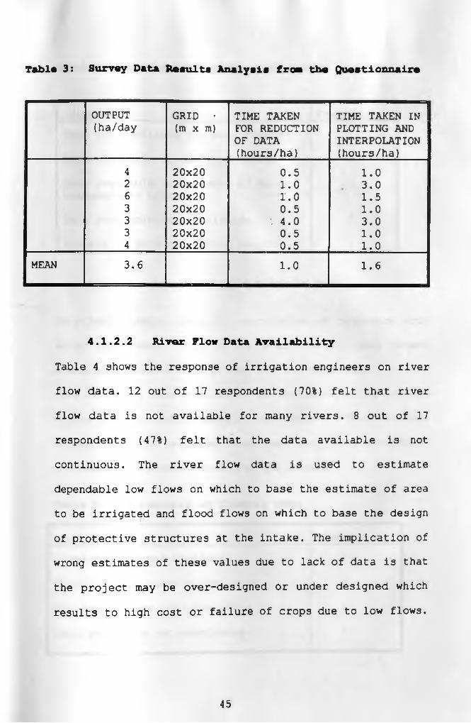
Tablt 3: Survey Data Reaulta Analysis fro* the Questionnaire
OUTPUT(ha/day
GRID • (m x m)
TIME TAKEN FOR REDUCTION OF DATA (hours/ha)
TIME TAKEN InH PLOTTING AND INTERPOLATION (hours/ha)
4 20x20 0.5 1.02 20x20 1.0 3.06 20x20 1.0 1.53 20x20 0.5 1.03 20x20 '.4.0 3.03 20x20 0.5 1.04 20x20 0.5 1.0
MEAN 3.6 1.0 1.6
4.1.2.2 River Flow Data Availability
Table 4 shows the response of irrigation engineers on river
flow data. 12 out of 17 respondents (70%) felt that river
flow data is not available for many rivers. 8 out of 17
respondents (47%) felt that the data available is not
continuous. The river flow data is used to estimate
dependable low flows on which to base the estimate of area
to be irrigated and flood flows on which to base the design
of protective structures at the intake. The implication of
wrong estimates of these values due to lack of data is that
the project may be over-designed or under designed which
results to high cost or failure of crops due to low flows.
45

Table 4: Availability of River Flow Data
Responce FrequencyData not available for many rivers 12
Data available in district office 2
Data available in Ministry of Water headquarters offices . 5 i
Data available not continuous 8
Process of data collection lengthy
4.1.2.3 Availability of Climatic Data
Detailed climatic data for calculation of reference crop
water requirement (ET0) is not available for many scheme
areas. The data available may not be continuous
(See Table 5). This results to the designers using average
values given in design manuals (See Table 8) . These average
values are for a broad area and may not accurately
represent the actual values for the scheme.
Table 5: Availability of Climatic Data
Response FrequencyClimatic data not available 8
Climatic data readily available 5
Pan evaporation data available 2
Data available not continuous 7
46

88% of the respondents felt that cropping calendar is not
prepared or decided upon during process (see table 6). this
means that an average value of crop coefficient is used for
calculation of crop water requirement as seen in table 7.
Crop water requirement vary over the growing season and the
peak water requirement is used during the design process,
however in many cases this is not used, an average value
given in manuals is used (see table 8).
Table 6: Preparation of Cropping Calendar
Response FrequencyNot done at all 6Sometimes is done 9Done for all schemes 2Total 17
Table 7: Determination Crop Coefficient
Response FrequencyCalculated from cropping patern 1Use average value from manuals 16Total 17
47

Table 8: Calculation of Crop Water Requirement
Response FrequencyCalculated from climatic data 4
and cropping patternUse pre-determined values from
manuals 13Total 17
Rainfall data is available for many scheme areas (See Table
9). For areas without rainfall records, figures from
similar ecological zones are used.
Table 9: Availability of Rainfall Data
Response FrequencyData not available 0
Data Readily available 2
Data Available for some stations 13
The data is not continuous 2
4.1.2.4 Other Design Activities
The following are other design activities for small scale
irrigation projects.
a) Establishing maximum irrigation interval;
b) Establishing the number of possible groups;
c) Canal layout;
d) Drainage system layout;
e) Design of the field irrigation system;
f) Generating canal ground profile;
48

g) Determination of dimensions of the canals;
h) Locating the canal longitudinal profile and
drop structures- on the ground profile;
i) Determination of the dimensions of the structures;
j) Determination of the bill of quantities; and
k) Economic analysis.
Table 7.3 in the annex shows the results of the ranking of
the above design activities according to the time taken, in
a descending order. Each activity is represented by the
corresponding letters as shown above. Table 10, below
shows the results of the analysis of the ranking done by
the engineers. It shows the score for each of the activity
(shown on top of the row and represented by the letters as
shown above) for each rank. The last row shows the total
score for each design activity.
Table 10: Design Activities Ranking Analysis
Rank Score Score for Design Activitya b c d e f 9 h i j k
1 11 0 0 44 0 11 22 22 11 33 22 222 10 0 0 10 10 0 40 10 20 40 10 303 9 0 27 36 18 0 9 9 36 9 18 04 8 0 0 8 16 8 16 0 32 24 24 85 7 7 21 14 7 14 0 21 7 0 21 76 6 12 0 18 12 0 18 12 0 18 0 67 5 5 5 0 5 20 5 5 5 0 5 258 4 8 4 0 4 4 8 12 0 4 16 49 3 15 0 3 6 9 3 3 3 0 3 310 2 0 12 0 6 0 0 2 6 2 0 2 }11 1 4 3 1 1 3 1 2 0 0 0 o
Total 51 72 134 85 69 122 98 120 130 119 107
The resulting ranking order, starting with design activity
49

which takes most time during design, relative to others is
as shown below has been extracted from Table 10, according
to the scores.
1) Canal layout (c);
2) Determination of the dimensions of the structures (i);
3) Generating canal ground profile (f); '
4) Drawing the canal longitudinal profile (h);
5) Determination of the bill of quantities(j);
6) Economic analysis of the project (k);
7) Determination of dimensions of the canals(g);
8) Drainage system layout(d);
9) Establishing the possible number of groups(b);
10) Design of the field irrigation system (e); and
11) Establishing maximum irrigation interval (a).
From the ranking order, it shows that the design activities
that take most of the time of the designer corresponds to
the areas of the design identified by the panel members as
problem areas. The comments of the engineers for each
activity are shown in Annex 4.
Most of the engineers felt time was a major constraint for
most of the activities. Most of the activities either
involves trying various alternatives or the iterations to
find the various parameters are repetitive. The engineers
after making few trails, gives up on trying further. These
50

results in unfinished designs or poorly calculated
dimensions. Another constraint mentioned is that there is
no clear design criteria 'and some design activities require
rule of thumb. Lack of experience was also mentioned as
another constraint.
4.2 EVALUATION OF MIDAS
Table 11 shows the various design activities and an
indication of the activities undertaken by MIDAS and those
undertaken by other packages. It also shows the design
activities where no package was identified to accomplish.
MIDAS does not handle the following major surface
irrigation design activities
analysis of hydrological information to establish
the design low flows and flood flows;
frequency analysis of rainfall data to determine
probable rainfall for determination of effective
rainfall;
determination of irrigation water requirements;
and
field irrigation systems.
For these design activities it means the designer will have
to go out of MIDAS to do them using other packages or do
them without using the computer.
51

%, /ER 31TY OF NAIROBI LIBRARYTable 11: Design Activities and Packages for them
Design Activity Undertaken by MIDAS Other Programs
1 Production of topographical •
Hap
(i) Reduction of survey data Done by DGH in
(ii) Interpolation and KIDA3
Drawing
2 Hydrological analysis
(i) Prediction of flows Hyrrom
(ii) Frequency analysis of HYFAP
flows
(iii) Probable rainfall PARADIGM
determination
3 Determination of water
requirement
(i) estimating ET0 and ETC - CROPWAT, CRIWAR, ETREF,
IRSIS, CWRTABLZ
(ii) determination of - CROPNAT
effective rainfall.
4 Scheme layout. Done through MIDAS
5 Design of field irrigation
systems
(i) Basins - BAS CAD
(ii) Border strip - BICAD
(iii) furrows - HOKE
6. Channel design
(i) determination of Done through MIDAS PROFILE,CID,DORC, CANDES
dimensions
(ii) Production of Done through MIDAS CID,CANDES
profiles
7. Structures' design DoneThrough MIDAS WZIRDES
8. Determination of bill of NONE
quantities
9. Economic analysis of the NONE
project
52

Table 12 shows the time taken for the various design
activities both by use of MIDAS and when not using
thecomputer. It is only the design activities carried out
by MIDAS that were compared. Some steps have a number of
sub-activities lumped together. It was not possible to
separate them as MIDAS handles them simultaneously.
Production of structures' inventory was not included as it
is instantaneously done using MIDAS. Design of the drainage
system was also not included as MIDAS only allow comparison
of run off and drain capacity but doesn't assist in design
of drainage system.
Except for design of structures, MIDAS design takes shorter
time than design without using the computer. For
structures' design if during the design of canal, the water
levels are well adjusted to provide enough head at the
structures point, MIDAS design would have been faster. The
quick process in these design activities, allow many trials
to be made of the design activity and by so doing high
quality (accurate) design is possible by the use of MIDAS.
The detailed evaluation of each design activity is as
discussed below.
53

Tabla 12: Tin* Taken on the Design Activities
Design Activity Time Taken
• MIDAS Design Process (hours)
Normal Design Process (hours)
1. Determination of scheme layout
20 24
2. Preparation fordetermination of canal ground profiles and production of the profiles
5
3. Canal design and location of drop structures and canal profiles on the ground profiles
15 54
4. Design of structures 3 1
4.2.1 Scheme Layout
The normal layout process (without using MIDAS) took a
longer period than use of MIDAS. However, much time had
been spent thinking of the layout before the use of MIDAS
so that if one started with MIDAS it would have taken more
time than the time shown.
The use of MIDAS allowed better positioning of canals by
the use of slope arrows and quick generation of ground
profiles (See Figure 2) . Through the use of AUTOCAD
commands for editing the design, high quality work
(neatness) was possible. The quick determination of the
lengths of canals and drains makes it possible for
different possible alternative layouts to be produced and
compared. This would solve the problems of scheme laying
out noted in section 4.1.1, the slope of the scheme area
not well understood, no alternative layouts considered,
54

canals in fill, the farmers taking water directly from the
main canal and the layout not well done.
The resulting layouts are shown in figures 7.1 to 7.3 in
the annex. Layout 2 was chosen. Figure 3 and Figure 4
resulting group layout and canal and drain layout
slope arrows.
shows
with
55

UJ
TT
U
(MO.
TT “1--1--T"•07.** M U U i n . « l
T TW.U ~2m
Figure 2 - Ground Profile of Proposed Canal

Figure 3 - Irriga tion Group Areas

F ig u r e 4 - C a n a l A n d D r a in L a y 0 l

4.2.2 Canal Profiles
From Table 12, the generation of the ground profile for the
canals took five hours with MIDAS and 18 hours for normal
design process. The process of marking the straight
sections of the canals and interpolating to find the levels
at the end of the section is the most tedious part of the
whole process for normal design. This has resulted to
designers leaving the generation of the profiles. This can
be seen from the comments of the panel members in section
4.1.1. The defining of the canal net work (See Section
2.4.5.) in MIDAS is the only step that takes time for canal
profile generation.
MIDAS uses more information for generation of ground
profiles. Each reach of the canal is divided into 20 m
sections and the levels at the ends noted. This makes the
resulting profile accurate. This can be seen for canal T4
Figure 7.8 and Figure 7.14. The canal generated normally
shows a gradual fall for the first 300 m while for the
canal generated by use of MIDAS shows a rise, especially at
chainage 220 m. The length of the canal generated without
use of MIDAS is 1020 m long while that generated by MIDAS
is 1034 m.
Once the canal network has been defined the generation of
the ground profile is fast and produces similar profiles.
59

For normal design to get another profile of the same canal,J|L
it will mean repeating the whole process of canal ground
profile generation.
4.2.3 Canal Design
The canal design process and incorporation of the design
and drop structures on the canal ground profile took 15
hours for MIDAS design and 54 hours for normal design
process. In normal design process, the determination of the
dimensions for the canal takes time as it involves trial
and error method (Newton Raphson Iteration) to determine
the right value of bed width and normal depth. Drawing the
profile for the designed canal also takes more time as
noted in Section 4.1.2 by the engineers. This step of the
design is often poorly done as shown in Section 4.1.1.
The MIDAS process of this step is fast. The editing tools
in MIDAS assists in adjusting the water levels in the canal
by adding, removing, changing or moving drop structures.
Check structures can also be added. This means the right
command can be achieved and improve the design of
structures due to increased head available. It also
increases the design accuracy of the canals. This can be
seen for canal T1 where it has three reaches of 0.008, 0.003
and 0.009 bed slope for normal design and 0.003 and 0.008
60

for MIDAS design (See Figure 7.5 and figure 7.11 in the
annex).
The complete canal design for MIDAS process is shown in
Figure 7.4 to Figure 7.9 while for normal design is shown
in Figure 7.10 to figure 7.15 in the annex. '
4.2.4 Design of Structure
The results of structures design using MIDAS are shown in
Figure 5 while the dimensions and water levels resulting
from normal design are shown in Table 13.
The design using MIDAS took more time than the normal
design process, this is attributed to more time being taken
up by redesigning the canal to get the right head to allow
the crest length to be within the cross-section of the
canal.
Comparing the available headloss and the resulting crest
length of the outlet weir, a discharge coefficient of 1.60
is used for the discharge equation. This coefficient is for
rectangular weir (MoA, 1989). A rounded weir is commonly
used in Kenya with a coefficient of 1.75. The assumption is
that the rectangular weir will wear off to rounded weir
finally.
61


Tabla 13: Canal Structani for Boi Darlgn
Structurn Canal Bad*lath
(■)
full Supply Lav.(■)
Bad laval
(■)Craat laval
(a)
Malr Laaqtn
(a)
O f f t a k e 1 Main 0.5 98.40 98.10T1 0.3 97.83 97.89 98.30 0.24Continuing 0.5 98.27 98.00 98.30 0.95
Offtake 2 Main 0.5 98.14 97.85T2 0.3 98.03 97.89 98.04 0.24Continuing 0.5 98.04 97.76' 98.04 0.71
Division MAIN 0.5 96.32 96.19I Box T3 0.3 96.18 96.02 96.27 0.67
T4 0.3 96.26 96.12 96.27 0.671------------- T5 0.3 96.27 96.08 96.27 0.67
4.3 IMPROVEMENT OF MIDAS
This has been a continuous activity during the time of the
project. The identified improvements were used by Overseas
Development Unit (ODU) of Hydraulic Research to improve the
package. Some of the improvements identified have been
incorporated into the package while some are still being
incorporated. Suggestions on how the improvements are to
be made have also been provided. The major changes required
are shown below.
4.3.1 Scheme Layout
The layout process for the initial package was meant to
produce regular irrigation groups (rectangular and
triangular) and canals with few reaches. The farmers in
small scale schemes in Kenya have fixed farm boundaries
which may be irregular. The layout commands should be in
63

such a way as to allow irregular groups with group
boundaries following the farm boundaries. The canals should
also follow the farm boundaries. The commands should allow
working with many canal reaches especially for the main
canal.
Schemes in Kenya are managed and operated by the farmers
themselves. This calls for a group size that will allow
easy group communication and organisation. A group size of
10 to 30 farmers is recommended (MoA, 1987) . A check on
group size is required.
4.3.2 Calculation of Water Requirements
The field irrigation system used in the initial package was
furrow irrigation, the water supply method used was mainly
rotation to the groups. In kenya basin and furrow
irrigation are used. The farmers are left to decide on the
sizes of the basins and furrow with assistance from the
field irrigation staff. The program needed to be changed
to accommodate these requirements, continuous flow to the
group and rotation flow within the group is practised in
small Scale Irrigation Schemes.
The program calculates the flow to the group assuming that
64

the whole area is to be irrigated. For small schemes in
Kenya, farmers irrigate a portion of their holding. The
area to base the calculation of the flow should be the
irrigated area per farmer multiplied by the number of
farmers in the group. The set up of the program assumes
seven days irrigation per week. Most of the farmers do not
work on Sundays. The number of irrigation days per week
should be left open. This will mean the group flow (unit
flow) will be different from the one for seven days.
4.3.3 Canal and Structures Design
During the evaluation process, during canal design, it was
hard to remember inputs previously used for canal design.
This becomes a bigger problem when a different person is
editing the design or writing the design report. A file to
hold the inputs (bedslope, bedwidth, side slope, the flow,
freeboard, drop height and Mannings KJ should be created
during the design. It should be possible to update the file
during editing.
During the design of structures, equation 5 and orifice
discharge formula shown below are used.
Q = CA (2gh)0,5 [6]
Where Q = Discharge through the orifice (m3/sec),
65

A = Cross sectional area of orifice opening (m2), C
* Discharge coefficient, and H = Head over the
orifice (M) .
For submerged flow, C is 0.6 for rectangular orifice and
0.65 for free flow rectangular orifice (MoA 1989). In MIDAS
submerged flow is assumed which may not be the case all the
time. The program should be changed to allow for different
shapes of orifice and for both submerged and free flow
conditions.
4.3.4 Inventory of Structures
The following weaknesses were identified during the
evaluation of MIDAS
For orifice type of offtake, crest level and area
of the orifice were not shown;
The orifice option was not working at all for the
division box; and
For miscellaneous structures on the canal, it
does not give the names. It terms them as unknown
structures yet when inserting them one specifies
whether a flume or culvert.
66
UNIVERSITY O F NAIROBI LIBRAR'4.3.5 Calculation of Cut and Pill for Canala
In MIDAS, during the canal design, cut and fill are
calculated for each reach of canal. The cumulative cut/fill
is also calculated. The figures given for each reach do
not represent the actual cut or fill but is the net. In
small scale irrigation projects what is important is how
much digging (cut) will be required and how much soil will
be imported. The program should be changed to give the
volume of cut and the volume of imported soil for the fill.
The detail procedures on how these quantities could be
calculated are shown in Annex 5.
4.3.6 Survey and Input of Existing Features' Data
The land surveying programs used in Digital Ground Model
(DGM), which forms a part of MIDAS can only be used to input
and process Radial and tacheometric survey data. In Kenya
many survey teams use engineers level and plane table for
surveying. From Section 4.1.2.1 it was established from
engineers that the average time for reduction and plotting
of maps takes 2.6 hours per hectare. So for a large scheme
the time taken in the office on preparation of maps is much.
Programs that will allow input and processing of survey data
done with the engineers level and plane table would reduce
67

the time taken in preparation of maps. Details on how to do
the field survey and the methods to calculate the data are
shown in Annex 6.
The Digital Ground Model does not have the capacity to sort
out the survey data to produce separate XYZ files for the
existing details. A separate program could be prepared to
sort out the information. During the surveying these details
should be identified and identification recorded. The data
should be put in a spread sheet and sorted out using the sort
facilities in these programs according to identification,
separate XYZ files should be prepared and copied to DGM. The
DGM will be used to prepare DXF files (Files used by AUTOCAD
to transfer information from DGM). These will be imported to
AUTOCAD for the preparation of the details on the map. The
detailed procedure is shown in Annex 5.
4.4 Adoption of Computer Aided Design Technology
This is a new technology being introduced to the irrigation
designers.The major constraints are on training of the staff
and supply of the equipment and their servicing.
Only the head office has been provided with the necessary
hardware for the computer aided design work. It is hoped that
the provincial offices will be provided with the equipment
68
the main hardware require for a smooth running design office
are
computer;.
Digitizer (tablet); and
Plotter.
The main software required are .
Autocad
_ Digital Ground Model or G.I.S
Minor Design Aid Software; and
Other support software such as spread sheets.
The initial training of the users of the software was done
by the ministry of Agriculture in conjunction with Overseas
Development Unit of Hydraulic research. The main areas that
require training are general software operation,
Autocad,Digital Ground Model, Digitization of the data into
the computer, and minor design Aid software. The main
constraint is the continuing of the training for the users
of the software.
69

5.CONCLUSIONS AND RECOMMENDATIONS
5.1 CONCLUSIONSThe shortcomins in the IDB irrigation projects' designs wereidentified as:1 There are delays in completion of design documents;2 Evaluation of design documents revealed that some of
the designs that are prepared are normally not complete and the calculations not thoroughly done due to repetative steps;
3 The operational requirements for the schemes are often not properly met e.g low command area due to low water level, farmers taking water directly from main canals, the layout not the best option and too many farmers per group;
4 For many schemes design data on river flow and climatic information is usually not available. This results to use of average values and as a result the scheme is under-designed or over-designed;and
5 There is no clear design procedure for the various irrigation methods as used in smallholder irrigation such as small basins and short furrows irrigation.
Computer aided design through Minor Irrigation Design Aid Software was found to have the following :
1 It handles design steps that takes most time due to repetitive procedures such as canal design, generation of ground profile and plotting of the map and is faster than normal design process; and
2 Accurate and neat output is possible from MIDAS as compared to normal design.
70
However it was found to have the following weakness:1 It does not assist in processing of river flow data,
rainfall data and climatic data;It does not assist in calculation of crop water requirements; and
3 It does not assist in the design of field application method such as basins and furrows.lt does not incorporate structural design.
5.2 RECCMMEDATIONS
1 The survey data input method in MIDAS should be expanded to include surveys done with plane table and engineers level. Method of input of information on existing features such as farm boundaries, rivers, canals and homesteads should also be devised.
2 A way of linking MIDAS with other packages to be used on design activities not handled by MIDAS is required. These packages could be CROPWAT, BASCAD SIRMOD and any package for analysis of hydrological and climatic data.
3 The surveyors should be taught how to carry out field survey in a way that meets the data requirements of MIDAS. ‘
4 A study on small basins and furrows as used in sma.. s irrigation in Kenya is required to establish suitability and suggest design consideration.
71

6 REFERENCESBannister, A. and Raymond, S. (1984) . Surveying, English Language Book Society, Longman
Bassett,D.L. (1983). Hydraulics of surface irrigation : In Design and Operation of Farm Irrigation Systems, ASAE, Michigan, America
Booher L. J. (1974). Surface irrigation, F.A.O., Rome
Boonstra J. and Jurriens M. (1988) . BASCAD. A Mathematical Model for level basin irrigation, ILRI, Wageningen, The Netherlands
Bos, M. G and Nugteren, (1983) . On irrigation efficiencies, ILRI, Netherlands.
Bowles, J.E (1984). Physical and Geotechnical Properties of Soil, McGraw Hill Book Company,New York.
Chow, V. T (1973). Open Channel Hydraulics, McGraw - Hill Book Company, Singapore.
Chow, V. T. (1988) . Applied Hydrology, McGraw - Hill Book Company, Singapore.
Domingo, F.T. (1986) . Farm level effects of Irrigation, Systems Design and Operation Problems, In irrigation design for management, Asian Regional Symposium, ODU, Hydraulic Research, (UK).
72

Doorenbos, J. and Pruitt, w. 0 (1977) . Guidelines forPredicting Crop Water Requirements, FAO, Rome.
Douglas, L. and Vermilion, (1989). Second approximations: Unplanned Farmer Contribution to Irrigation Design, ODI/IIMI. Irrigation Management Paper 89/2C.
Gibb at al, (1987). Small Scale Irrigation Development, Inventory and Study of Traditional Irrigation Furrows in Elegeyo-Marakwet District. Volume I, MoA., Kenya.
Ground Water Survey Ltd., (1992) . Soil Site Investigation and Irrigation Suitability Assessment, Gambela Irrigation Scheme,S.I.D.P., Kenya.
Horst, L. (1990). Incompatibility between Exogenous Design Culture and Farmers' Perception, In Design for Sustainable Farmers Managed Irrigation Schemes in sub-Sahara Africa,
Hydraulic Research, (1991). Small Scale Irrigation Development in Africa, ODU Bulletin number 22 Hydraulic Research, Wallingford, (UK) .
Hydraulic Research, (1993) . MIDAS user guide for Ministry of Agriculture, Irrigation and Drainage Branch, Hydraulic Research, Wallingford.
Institute of Hydrology, (1992a) . HYRROM - Hydrological Rainfall Runoff Model,Institute of Hydrology, Wallingford, (UK) .Institute of Hydrology, (1992b) . HYFAP - HydrologicalFrequency Analysis Package, Institute of Hydrology Wallingford, (UK) .
73

Jurrians, M. (1993). Computer programs for Irrigation Management - The State of the Art, ODU Bulletin Issue 27,Hydraulic Research, Wallingford, (UK).
Kaophuis, J. J. (1993). Land and Water Use Computer Programs for Personal Computer, L & W Version 2.0 Euroconsult, Netherlands
Khuahalani, K.B. and Khuahalani,. M. (1990). Irrigation Practice and design, volume 11, Mohan Primlani,New Delhi
Kohlhaaa, C. A, and Nicolau, A. M. (1985) . Present Status,of Computer-Aided Analysis, Design and Drafting (CAADD) Application in Irrigation and Drainage, ICID Bulletin, January, 1985 Vol 34, No. 1 Pg. 15 - 19.
Lenaelink, K. J. and Jurrion3 , M. (1993) . An Inventory of Irrigation Software for Micro-computer, ILRI, Wageningen, The Netherlands.
L«a, N. (1990). PARADIGM (Parameters for Rainfall Distribution in a Gamma Model), Hydraulic Research, wallingford, (UK).
Ministry of Agriculture, (1986a) . Scheme Identification Manual, MoA/IDB, Kenya.
Ministry of Agriculture, (1986b) . Guidelines - Small holder Irrigation Projects in Rural Development, MoA/IDB.
Ministry of Agriculture, (1987) . Scheme Design manual, MoA/IDB,Kenya.
Ministry of Agriculture, (1989) . Structures - Manual for
74

senior IDB staff on division structures, MoA/IDB, Kenya.
Ministry of Agriculture, (1990). Planning Workshop for Small Scale Holder Irrigation and Drainage Development in Kenya during the 6th Development Plan Period, MoA/IDB, Kenya.
Moejes, J. W. (1990). Design problems in Small holder Irrigation with reference to Kenya,University of Nairobi, Kenya.
Pazvakavambwa, S. (1984) . Relationship between design of Smallholder Irrigation systems and their subsequent operation criteria : In African Regional Symposium on OnSmallholder Irrigation, University of Zimbabwe, Harare.
Speelman J. J. (1990) . Design for sustainable Farmers Managed Irrigation Schemes in Sub-Saharan Country, ODI/IIMI.
SSIDP, (1989). Smallholder Irrigation Development Project Position Paper, Volume 1, MoA/IDB, Kenya.
Smith M. (1992) . CROPWAT - A computer program for irrigation Planning and Management, Irrigation and Drainage Paper 4 6,FAO, Rome.
Tiffon, M. and Guston, H. (1983). Alternate design Concepts for irrigation systems, ODI Irrigation Management net work paper 89/lc.
Withers and Vipond, (1988) . Irrigation design and Practice, BT Balsford Limited, London.
75

ANNEX 1 - DETERMINATION OP WATER REQUIREMENT
A - CLIMATE
Table 1.1: Shows climatic data for Isiolo Metecrogica. Station (No. 8937/003) which is 17 km. west of the project area. Rainfall record (Daily) was available for the same station for 17 years (See Table 1.2). The climatic data was analysed using CROPWAT package, according to the FAO adapted Penman-Monteith approach (Smith, 1992)
The yearly evapotranspiration of the area is 2678 mn with the highest evapotranspiration being 8.6 mm/day in August. The area receives rainfall with 80% reliability of 340 mm occurring in two seasons. The long rainy season from March to May and short rainy season from October to December.
B - PEAK NET IRRIGATION WATER REQUIREMENTS
The crop water requirement (ETC) is given by
ETCWhereETCETCKc
KCET0
Crop Water Requirement (mm/day) Reference crop water requirement (mm/da/)Crop Coefficient
The crops to be grown in the scheme are ma.~e, beans, tomatoes and onions. Table 1.4 shows crop coefficient length of each growth stage for these crops.The effective rainfall shown in Table 1.3 was ^a^u using CROPWAT package. In this package four met..o<<. of
76
determining effective rainfall are used. These are Fixed percentage of rainfall;Dependable Rain (emperical form);Emperical formular (locally dev.); and USDA Soil Conservation service method.
Dependable Rain method was used. It combines both determination of 80% reliability and detemination of effective rainfall. The input is' the average monthly rainfall. Acording to Smith (1992),. it is based on analysis carried out for different arid and Sub - humid climates.The test scheme, Gambela is in arid climate.The annual effective rainfall of the scheme area is 348 mm. According to Ground Water Survey Ltd (1992) the ground water in many parts of the scheme is below one meter. The contribution of ground water for the crop water requirement was neglected. Table 1.5 - Table 7.1.12 shows the crop water requirement as calculated using CROPWAT. The peak net irrigation requirement varies for various crops and an average value of 8.00 mm/day was taken for design.
77

Table 1.1: Reference Evapotranapiration (ET,) according to Penman-Monteith method
Country: Kenya Meteorological Station: Isiolo (8937/003:
Altitude:3621M Coordinates: 0.35 N.L 37.35 e .LMonth Max.
TempC
Min.TempC
Humidity%
Wind run Km/day
SunshineHours
Sol.Rad. MJ/day
KT.-PenaenM/day
January 30.8 15.7 48 334 12.1 27.1 7February 32.4 16.3 45 334 12.1 28.1 7.4March 31.7 17.6 50 401 12.1 28.6 7.8April 30.1 17.8 57 401 12.1 27.7 7.1May 29.9 17.8 56 534 12.1 26.3 7.3June 29.5 16.9 53 623 12.1 25.3 7.6July 28.9 16.3 54 668 12.1 25.7 7.6August 29.4 16.5 52 445 12.1 27 7.2Septeaber 30.8 16.9 49 623 12.1 28.1 8.6October 30.9 17.6 51 445 12.1 28.1 7.8loveaber 28.6 16.6 60 289 12.1 27.3 6.3Oeceaber 29 15.5 59 289 12.1 26.7 6.2
Tear 30.2 16.8 16.8 449 12.1 27.2 2678
78

Table 1.2 Rtt I it f n 1 I dntn Tor I
Irr-,— t January february march april may ju n e .
1974 41.9 47.6 54.0 125.4 31.3 0.01975 27.7 0.0 39.9 147.8 24.4 0.01976 44.4 104.5 33.6 102.1 16.0 22.71977 104.9 0.0 88.2 193.4 31.0 0.01978 45.2 45.4 170.8 177.4 0.0 0.01979 140.5 54.9 82.2 141.2 7.5 2.31980 0.0 20.0 46.8 125.5 62.1 0.01981 22.5 7.9 101.4 66.2 98.8 0.01983 28.0 37.1 24.2 195.1 13.4 0.01984 3.3 12.2 38.0 81.0 0.0 0.01985 47.2 12.5 109.4 146.0 8.9 17.81986 1.2 12.9 114.7 180.7 15.8 16.81987 18.6 5.8 76.2 204.1 3.3 59.21988 28.3 18.8 117.4 123.1 15.3 9.61969 33.4 4G.8 99.8 118.8 33.2 0.01990 47.8 110.4 252.7 161.3 23.7 0.01991 72.6 8.0 112.8 54.9 21.0 0.0
AVERAQIE 41.6 32.0 91.9 137.9 23.9 7.JB

In Hp I . n t« t | on t 0 9 3 7 /Ou:i» .
august sept. October nov. dec. TOTAL
2.5 0.0 0.0 52.4 108.7 57.2 521.012.5 0.0 19.3 34.2 137.5 35.5 478.8
0.0 1.3 0.0 12.0 123.0 173.8 633.40.0 0.0 21.4 114.2 97.4 45.2 695.70.0 0.0 16.0 124.6 144.6 197.1 921.10.0 0.0 • 0.0 22.4 201.8 64.8 717.60.0 0.0 0.0 28.8 208.3 54.2 545.70.0 0.0 4.5 34.0 86.2 38.9 48Q 40.0 42.8 3.9 16.6 96.4 122.2 5 ’9.70.0 0.0 12.8 70.7 290.0 27.2 5 15.20.0 0.0 5.6 35.6 151.6 46.4 5M1.00.0 0.0 0.0 89.7 185.0 76.1 6^2 90.0 0.0 46.9 28.0 138.7 67.6 6 m .4
11.5 1.6 13.5 46.4 165.6 154.4 705.54.5 0.0 19.8 158.4 243.6 138.2 896.50.0 0.0 0.0 236.7 180.0 164.6 111123.5 0.0 0.0 82.3 151.4 159.3 665.82.0 2.7 9.6 69.8 159.4 95.5 673.9

M L S 1.3: Iffectire Rainfall according to ^>irical For*!* IMdBMJnc)
ET„ Average Rainfall nt/month
Ef f .Rain mm/month
January 7.0 41.6 15.0February 7.6 32.0 9.2March 7.8 91.9 48.5April 7.1 137.9 85.3May 7.3 23.9 4.3Jane 7.6 7.6 0.0July 7.6 2.0 0.0August 7.2 2.7 0.0September 8.6 9.6 0.0October 7.8 69.8 31.9Sovember 6.3 159.4 102.5December 6.2 95.5 51.4
Tear 267 673.9 348.17.6
Table 1 . 4 : Crop Data
CROP GROWTH STG. INITIAL DEVEL. MID LATE TOTAL
Seans Length(days) 20 30 40 20 110Coeff. 0.35 - 1.03 0.7
Maize Length (days) 25 40 45 30 140Coeff. 0.4 _ 1.13 0.86
Onions Length(days) 30 40 50 30 150Coeff. 0.7 - 0.95 0.75 _ —
Tomatoes Length (days) 30 40 40 25 135coeff. 0.45 - 1.15 0.85
Source: Smith, 1992
80

lata Station: Zalolo ((937/003)
1 .3 : Crop Evapo transpiration and Irrigation Aeqnl raatif
Crop: Beans PlantingDate:
15March
Meat* Decade. Stage Coeff ETc ETc Eff. Rain Irreg. Irreg.Kc nm/day on/dec nm/dec am7 day aa/dec
March 2 init 0.35 2.73 13.7 8.1 1.11 5.6March 3 init 0.35 2.65 26.5 20.3 0.62 6.2April 1 in/dev 0.41 2.98 29.8 27.7 0.21 2.1April 2 dev 0.58 4.09 40.9 33.4 0.75 7.5April 3 dev 0.80 5.76 57.6 22.8 3.48 34.8May 1 dev/mid 0.97 7.04 70.4 9.4 6.10 61.0.May 2 mid 1.03 7.52 75.2 0.0 7.52 75.2May 3 mid 1.03 7.62 76.2 0.0 7.62 76.2June 1 mid 1.03 7.73 77.3 0.0 7.73 77.3Jane 2 mid/late 0.99 7.51 75.1 0.0 7.51 75.1Cune 3 late 0.87 6.57 65.7 0.0 6.57 65.7July 1 late 0.70 5.32 26.6 0.0 5.32 26.6
Total 635.0 121.7 513.3
Sable l.(: Crop Xvapotranspiration and Irrigation Requirements
n 1mto Station: Zalolo (8937/003)
Crop: Beans Planting 15___________________________________________ Date: August
Month decade
stage Coeff.Kc
ETcmm/day
ETcmm/dec
Eff.Rain mm/dec
Irreg. mm/day
Irreg.on/dec
AugustAugustSeptemberSeptemberSeptember3ctoberOctoberOctoberNovemberNovemberNovemberDecember
231231231231
initinitin/devdevdevde/midmidmidmidmid/latlatelate
0.350.350.410.580.800.971.031.031.03 0.99 0.87 0.7
2.452.643.36 5.07 6.80 7.85 8.03 7.52 6.94 6.135.364.36
12.326.433.650.7 68.078.580.375.269.461.353.621.8
00002.96.49.617.8 29.3 239.231.811.9
2.452.643.365.07 6.517.217.07 5.74 4.002.21 2.18 1.98
12.326.433.650.765.172.170.757.440.022.121.8 9.9
Total 631.1 149.0 482.2
81

Cllaate Station: laiolo (8937/003)
Table 1.7: Crop >vapotran*piration and Irrigation “ijiuj.____ _
c m r Maize Plantingdate:
15-March
M U Decade Stage Coeff. ETcm/day
ETc. >e/dec
Eff. tola ■e/dee
trreg. Irreg
..T... 2 init 0.4 3.12 15.6 6.1 1.50 7.5xo.e i3 Init 0.4 3.03 30.3 20.3 1.00
1 init 0.4 2.93 29.3 27.7 0.16 1.42 dev 0.49 3.49 34.9 33.4 0.14 1.4Se*t — o»r 3 dev 0.67 4.83 48.3 22.1 2.55 25.5Dctotn: 1 dev 0.86 6.19 61.9 9.4 5.25 652.1Dc*.et»r 2 d«v 1.04 7.58 75.8 0.0 7.5a 75.1October 3 ■id 1.13 8.36 83.6 0.0 8.36 63.4+ r T T 1 eld 1.13 8.48 84.8 0.0 8.46 •4.4
2 mid 1.13 8.59 85.9 0.0 8.59 65.963.9W i r 3 Bid 1.13 8.59 85.9 0.0 8.59
1 ald/late 1.11 8.43 84.3 0.0 8.41 64.)> : « M r 2 late 1.05 7.95 79.5 0.0 7.95 79.3
3 late 0.96 7.19 71.9 0.0 7.19 71.9Jaa-uarv 1 late 0.88 6.34 31.7 0.0 .. 6.34 11.7
Total 903.7 121.7 762.0
Tabla 1.8: Crop Kvapotranapiration and Irrigation Raqoiraaanta
climate Station: Zaiola (SM7/003)
Crop: Maize Planti ngdate:
15August
Month Dec Stage Coeff.Kc
BTcmm/day
ETc nan/ d o c
Eff. Rain n a n / d a c
Zrraq■■/day
Xrreq am/dae
M archM archAprilAprilAprilMayMayMayJuneJuneJuneJulyJulyJulyAugust
initinitinitdevdevdevdevmidmidmidmidmid/latelatelatelate
0.40.40.40.490.670 . 861.041.131.131.131.131.111.05 0.96 0 .88
2.803.013.314.32 5.706.91 8 . 1 0 8.25 7.617.017.016.91 6.49 6.23 5.93
14.030.133.1 343.257.069.1 81.082.576.170.170.169.1 64.9 62.329.6
0.00.00.00.02.96.49.617.829.339.231.823.8 16.112.44.2
2.803.013.314.32 5.42 6.27 7.14 6.47 4.683.09 3.82 4.53 4.88 4.995.09
14.0230.133.143.234.262.7 71.464.746.830.938.243.348.849.923.4
Total 852.2 193.6 638.6
82
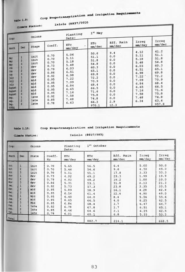
- u m f f ________________ Xrrlfl.ti-1. , Crop Xvaporran-i'fibli 1 • •4 . I.iolo (8937/003)
/•]<— to Station.
Table 1.10: Crop Xvapotranapiretion and Irrigation Raqviiracnant*
Cliaat* Station: Zalolo (892"7/003)
Crop: Onions Planting October
Month Dec State Coeff. Kc
ETCmm/day
ETCmm/day
Eff. Rainran/dec
Irraq on/day
Irraq ana/da c
1 init 0.70 5.65 56.5 6.4 5.00 50.02 init 0.70 5.46 54.6 9.6 4.50 45.03 init 0.70 5.11 51.1 17.8 3.33 33.31 dev 0.73 4.92 49.2 29.3 1.99 19.92 dev 0.79 4.92 49.2 39.2 1.00 10.03 dev 0.86 5.31 53.1 31.8 2.13 21.31 dev 0.92 5.73 57.3 23.8 3.35 33.52 mid 0.95 5.89 58.9 16.1 4.28 | 42.83 mid 0.95 6.14 61.4 12.4 4.90 49.01 mid 0.95 6.40 64.0 8.4 5.56 55.62 mid 0.95 6.65 66.5 4.0 6.25 62.53 Mid 0.95 6.84 68.4 3.7 6.47 1 64.71 late 0.92 6.78 67.8 2.7 6.51 65.12 late 0.85 6.46 64.6 2.1 6.25 62.53 late 0.78 6.01 60.1 6.8 5.33 53.3
882.7 214.1 668.5
Oct
Oct
OctBov
Bov
Bov
Dec.
Dec.
Dec.
Jan.Jan.
Jan.fab.Feb.
_feb.
T o ta l
83

Climate Station: Isiolo (8937/003)
table 1.11: Cxop Xvapotranspiration and Irrigation Requirement*
Crop: Tomatoes PlantingDate:
ISOctober
Month Dec Stage Coeff. Kc
ETc ‘ mn/day
ETcvmJ dec
Eff. Rain nm/dec
Irreq am/day
Irreq an /dec
O cto b er 2 init 0.45 3.51 17.5 4.8 2.55 12.7O cto b er 3 init 0.45 3.29 32.9 17.8 1.50 15.0R cveab er 1 init 0.45 3.03 30.3 29.3 0.10 1.0November 2 in/dev 0.49 3.06 30.6 39.2 0.00 0.0November 3 dev 0.63 3.88 38.8 31.8 0.69 6.9December 1 dev 0.8 4.99 49.9 23.8 2.61 26.1December 2 dev 0.98 6.05 60.5 16.1 4.43 44.3December 3 dev/mid 1.11 7.15 71.5 12.4 5.91 59.1Ja n u a ry 1 mid 1.15 7.74 77.4 8.4 6.91 69.1J a n u a ry 2 mid 1.15 8.05 80.5 4.0 7.65 76.5J a n u a ry 3 mid 1.15 8.28 82.8 3.7 7.91 79.1F e b ru a ry 1 mid/lat 1.12 8.29 82.9 2.7 8.02 80.2F e b ru a ry 2 late 1.03 7.83 78.3 2.1 7.62 76.2F e b ru a ry 3 late 0.91 6.98 69.8 6.8 6.30 63.0
T o t a l 803.6 202.9 609.2
Table 1.12: Crop Xvapotranspiration and Irrigation Requirement#
Climate Station: Isiolo (8937/003)
84

c. Estimation of Efficiencies
Small basin irrigation system will be practicsed in the scheme.
The flow in the main canal and group feeders will be in
rotation. According to Bo's and Nugteren (1982), intermittent
basin irrigation shows a constant application efficiency of
0.58 (See Figure 1.1). The flow to the group is 12 1/sec/ha for
the 0.28 ha which will be irrigated per farmer. From Figure
1.2, the estimated application efficiency is 0.66. This gives
an average application efficiency of 0.62. for design purpose
application efficiency of 0.6 was used. From Figure 1.3 the
distribution efficiency was estimated at 0.92 for the scheme
operation. The conveyance efficiency was estimated at 0.95
giving an overall efficiency of 52%.
85

Figure
Source :
FIGURE
FIEIO APPLICATION EFFICIENCY* 0 * vm / Vl
8 18 A v e r a g e v a l u e s f o r
39 r o g a t i o n p r o t e c t s
* ( e * c l u d < n g n e e p r o t e c t s )
__7 -
16 n e e p r o t e c t s
6 -
5 -
4 -
3 -
2 -
0 1
B A S I N F U R R O W BORDER s p r i n k l e r
STRIP
F I E L D I R R I G A T I O N m e t h o o
1.1: Field Application efficiency related toirrigation methods
Bos and Nugteren , (1983)
1.2
Source:
Influence of Flow Rate Per ha. Farm Plot on
Aplication Efficiency
Bos ar^ Nugteren , (1993)

FIGURE 1.3
Source
The Distribution Efficiency «* * Unction of Farm size ani Dominant soli type.
Bos and Nug teren . (1983 )
FIGURE .1 4Source :
- The Conveyance Efficiency as a function of Irrigable area.
Bos and Nugteren.(1983)
87

D. Gross Water Requirement
The fanners are to irrigate for seven days per week to utilise
the low flow in the river. The farmers will irrigate for 24
hours per day. The gross water requirement is given by
100 7 24
G.I.R = N.I.R * 0.116 * — * __ * __ * 7 1 1
E DPW HPD
Where G.I.R = Gross irrigation requirement (1/sec/ha),
N.I.R = Peak net irrigation requirement (mm/day), DPW -
Irrigation days per week, HPD = Irrigation hours per day, and
E = Overall efficiency.
At 8.0 mm/day net irrigation requirement, for 24 hour
irrigation the gross water requirement is 1.79 1/sec/ha. The
river is not gauged at any point near the point of abstraction.
Estimate of the flow done during the dry season using float
method, gave a flow of 0.090 m3. The Ministry of Water allows
a maximum of two third of available flow for extraction. This
means the available flow for extractin for irrigation is 0.060
m 3 . This is the flow that was used for design of the
irrigation system. 33.62 ha. out of 55 ha. scheme area, w:.. ce
irrigated for 24 hours irrigation equivalent to 0.28 per farmer
8 8

for the 120 farmers.
I Water Distribution
The scheme is to be divided into five groups having 24 farmers
per group (see figure 3 ) . The flow will be continous to each
group but within the group the flow will be rotated among the
farmers at a time. Each farmer will Irrigate for seven hours
with an irrigation interval of seven days.
The gross flow to each group is 0.012m3 . Net irrigation
application is 0.006 m3 which is equivalent to 56mm for the
seven hours on the 0.28 ha.per farmer, the irrgation interval
varies with the rooting depth which also depends on the crop
and growth stage.The farmers will organise themselves so that
for crops that require shorter intevals, they can be provided
with water for a shorter period but more frequent.
89

ANNEX 2 - CALCULATION OF CANAL DIMENSIONS USING
MANNINGS EQUATIONMannings equation is given by
Q A Kjn S1/2 R2/3 P .t .i j
Where Q = Flow in the canal (m3/sec), K. - Manningsroughness
coefficient (m1/3/sec), A = Wetted area (m2), S ■ Bed slopeof the canal (m/m), and R = Hydraulic radius (m).
Re-arranging the above equation we have
Q
A*R2/3 = ------ (7.2.2)
Km*S1/2
The expression AR2/3 is called the section factor for uniform
flow computation (Chow, 1973). In most calculations, the flow
in the canal is known. The roughness coefficient, can also be
estimated and bed slope fixed. The right hand quantity can be
known. Trapezoidal canal sections will be used.
90

Letting the quantity <2/KmS:/: whose value is known to be (,
then the following expressions will be used to determine me
bed width and normal depth of the flow in the canal. The wet* i
perimeter, wetted area and hydraulic radius for the sec: . n
shown in figure 7.2.1 are given by
A = (b+zd)d [7.2.3]
P = b+2 (l + z:)1/: d i'.2.4]
A
R = — =
[ b -i- zd] d[7.2.5]
b + 2 [1 + z: j;': d
91
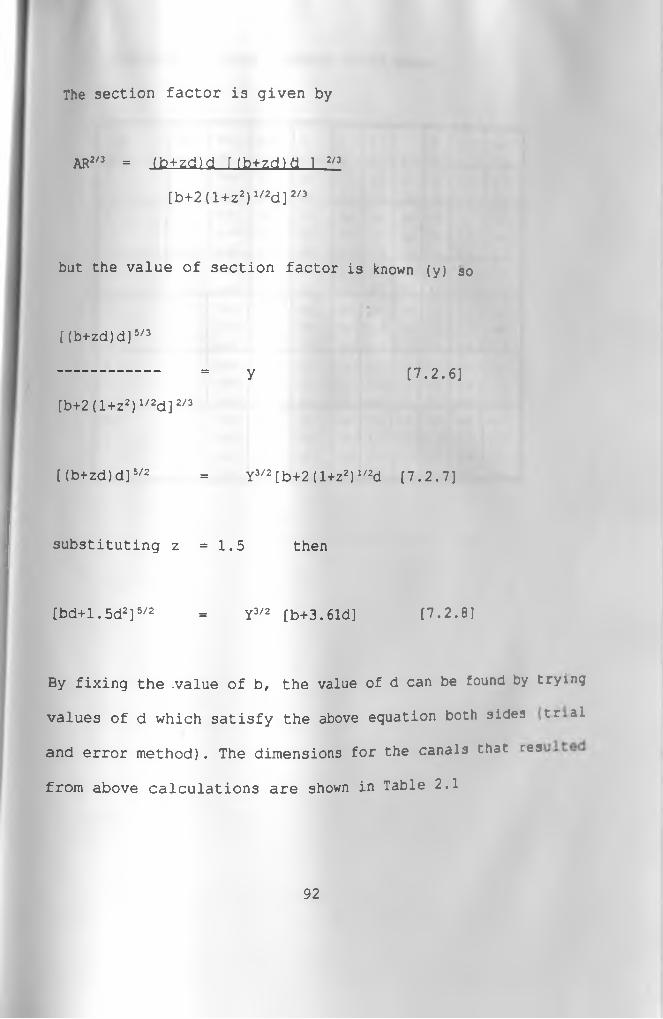
The section factor is given by
AR2/3 = (b+zd)d r (b+zd)fl 1 2/3
[b+2 (1+z2) 1/2d]2/3
but the value of section factor is known (y) so
[ (b+zd) d]5/3
----------- = y [7.2.6]
[b+2 (1+z2) 1/2d]2/3
[ (b+zd)d]5/2 = Y3/2 [b+2 (1+z2) 1/2d [7.2.7]
substituting z =1.5 then
[bd+1.5d2]5/2 = Y3/2 [b+3.61d] [7.2.8]
By fixing the .value of b, the value of d can be found by trying
values of d which satisfy the above equation both sides tr.al
and error method). The dimensions for the canals that res.,
from above calculations are shown in Table 2.1
92

Table 2.1: Canal design using Midas
ClMl
Ho
Reach
No.
Slope
m / m
Flow
1/seck;
, a/sec
b
a
d
■
s
a
f
ab
a*aj
1 1 0.008 12 15 0.3 0.11 1.5 0.1 0.21 0.332 0.003 12 15 0.3 0.14 1.3 0.1 0.24 0.22
2 1 0.01 12 15 0.3 0.1 1.5 0.1 0.2 0.342 0.003 12 IS 0.3 0.14 1.5 0.1 0.24 0.223 0.001 12 15 0.3 0.19 1.5 0.1 0.29 0.14
3 1 0.012 12 15 0.3 0.1 • 1.3 0.1 0.2 0.392 0.003 12 15 0.3 0.14 1.5 0.1 0.24 0.22
4 1 0.01 12 15 0.3 0.1 1.3 0.1 0.2 0.362 0.003 12 IS 0.3 0.14 1.5 0.1 0.24 0.22
3 0.002 12 15 0.3 0.16 1.5 0.1 0.26 •-
5 1 0.007 12 15 0.3 0.11 1.5 0.1 0.21 0.31
2 0.009 12 15 0.3 0.11 1.5 0.1 0.21 0.35
3 0.001 12 15 0.3 0.19 1.3 0.1 0.29 0.14
Main X 0.015 36 IS 0.5 0.13 1.3 0.1 0.23 0.63
2 0.001 36 15 0.5 0.27 1.5 0.1 0.37 0.23
3 0.001 48 20 0.5 0.32 1.5 0.1 0.42 0.24
4 0.001 59 20 0.5 0.36 1.5 0.1 0.46 0.24

Table 2.2: Parameters for normal canal design
Canal
Ho.
Ranch
No.
Slop#
■/a
Flow
1/sac
Ka
a/sac
b
■
d
■
s f
■
b
•
V_
a/ sac
1 1 0.0000 12 15 *0.30 0.11 1.50 0.10 0.21 0.32
2 0.0030 12 15 0.30 0.14 1.50 0.10 0.24 0.22
3 0.0090 12 15 0.30 0.11 1.50 0.10 0.21 0.32
2 1 0.0100 12 15 0.30 0.10 1.50 0.10 0.20 0.36
2 0.0060 12 15 0.30 0.12 1.50 0.10 0.22 0.29
3 0.0010 12 15 0.30 0.18 1.50 0.10 0.28 0.14
3 1 0.0120 12 15 0.30 0.10 1.50 0.10 0.20 0.36
2 0.0072 12 15 0.30 0.11 1.50 0.10 0.21 0.32
3 0.0030 12 15 0.30 0.14 1.50 0.10 0.24 0.22
4 0.0100 12 15 0.30 0.10 1.50 0.10 0.20 0.36
4 1 0.0100 12 15 0.30 0.10 1.50 0.10 0.20 0.36
2 0.0030 12 15 0.30 0.14 1.50 0.10 0.24 0.22
3 0.0090 12 15 0.30 0.11 1.50 0.10 0.21 0.32
4 0.0030 12 15 0.30 0.14 1.50 0.10 0.24 0.22
5 1 0.0100 12 15 0.30 0.10 1.50 0.10 0.20 0.36
2 0.0070 12 15 0.30 0.11 1.50 0.10 0.21 0.32
3 0.0010 12 15 0.30 0.18 1.50 0.10 0.28 0.14
Main 1 0.0100 36 15 0.40 0.16 1.50 0.10 0.26 0.43
2 0.0005 36 15 0.40 0.34 1.50 0.10 0.44 0.12
3 0.0005 4B 20 0.50 0.32 1.50 0.10 0.42 0.17
4 0.0030 20 0.50 0.23 1.50 0.10 0.33
94
ANNEX 3: QUESTIONNAIRE1. GENERAL INFORMATION
i) Name of the Province . . .
ii) How many schemes have you designed within theProvince....
iii) Of the schemes you have designed within-the Province orelse where within the country, indicate the number of
schemes you have designed under each category shown
below.
a) Furrow irrigation ............................
b) Wild flooding ................................
c) Basin irrigation ..............................
d) Combination of furrow and b a s i n ...............
iv) How often do you design (determine) the size of furrows
or basin. (Tick the correct one)
a) For every irrigation scheme designed...........
b) For a few schemes ............................
c) Not done at all ..............................
Survey Information
i) What is the average output of one surveyor in y°ur
Province (District)........ha/day.
ii) What grid do they use....... ...............miii) How much time is taken in getting the reduced levels
95

hours/ha
iv) How much time is taken for interpolation and plotting of
the contourMap.............. hours/ha
v) in accomplishing (iii) and (iv) . What are the major
constraints............................................
3. River Flow Para
i) Tick the appropriate statement about river flow data that
you think is true.
a) Data not available for many rivers..............
b) The data is not available in the district.......
c) Data available in Ministry of water's head
quarters........................................
d) The process of data collection is lengthy........
e) Data available is not continuous
ii) State the major constraint in determining the low flow
with the required reliability.................
iii) What is the major constraint in determining flood flows
for a required return period............
4. Determination of Water Requirement and Design FlSM
i) What method do you mainly use in determining crop water
requirement (ETC) . (Tick the correct one)
96

a) Calculation from climatic data and cropping
calendar
b) From Irrigation hand books and manuals
ii) In collection of climatic data, which of the following
statements apply (Tick)
a) Climatic data not available (temp.,humidity,
sunshine record, and radiation)...........
b) Climatic data is readily available........
c) Pan evaporation data is available........
d) Data available not continuous..............
iii) How often do you prepare a cropping Calendar for the
schemes (Tick)
a) Not at all..................................
b) Some times..................................
c) For all the schemes designed...............
iv) What value of crop coefficient (Kc) do you often use
(Tick)
a) Calculated value from the cropping
pattern......................................
b) An average value given in books............
(v) Tick the most appropriate statement for the rainfall
information.
a) The data is not available.....................
b) The data is readily available................
97
c) The data is usually available for some
stations......................................
d) The records are not continuous
vi) With all data available, what is the average time taken
for the following tasks.
a) Determination of ETo from climatic data
........... hours
b) Determination of crop -coefficient from cropping
Calender................... hours
c) Analysis of rainfall data to get effective
rainfall.................. hours.
The following are major design tasks and activities. Rank them
in order of the proportion of design time taken. Starting with
the task that takes most time and ending with the one that
takes least time.
a) Determination of maximum irrigation interval
b) Establishing the number of groups
c) Determining the position (location) of canals
d) Deciding on drainage layout
e) Determining the dimensions of basins and furrow
f) Generating canal ground profiles
g) Determination of dimensions of the channels
h) Locating the canal on ground profile and drop
98

structures and construction materials
i) Determining the dimensions of the required
structures and construction materials
j) Determining the bill of quantities
k) Economic analysis
Rank 1 2 3 4 5 6 7 8 9 10 11Activity - •
ii) For the first six activities state the major constraint
1................................................
2...........................................................
3.
4 ..................................................
5 .....................................................
6 ..................................................................................................................................
B. MAILING LIST FOR QUESTIONNAIREThe target group was irrigation engineer^ who have
involved in the design of small scale surface
schemes. A total of 31 questionnaires were sent
replied.
99

NAME STATION1. Kagiri A. W Nakuru2 . Kiragu G. M. Laikipia3 . Muiruri F. N. Kajjiado4 . Ogango P.D Elgeyo Marakwet5 . Omwenga G. J. PIU-Nakuru6 . Chepsoi PIU Nakuru7 . Omedi PIU Nyanza8 . Kapkiyai D. PIU Nyanza9 . Kiplangat W.C PIU Nyanza10. Maithya G. M PIU Nyanza11. Githae A. M. PIU Nyanza12. Kombo J. 0. PIU Nyanza13 . Asawo L.W. 0. PIU Nyanza14 . Kabok P. A PIU Nyanza15 . Ochieng J. 0. PIU Nyanza16. Muthigani P. M. Garissa17. Wairangu J. K. Garissa18. Onchoke O.W Meru19 . Njoka B. K. PIU Eastern20. Mbandi J. W. PIU Eastern21. Miya J. 0. PIU Eastern22 . Magero B. J. Isiolo23 . Maina B. M. Machakos24 . Mutavi S. M. Kirinyaqa25 . Simiyu J.A kiambu26 . Nderitu P. G. Nairobi27 . Nyanquti J. 0. N a i r o b i _________
28 Sifuma J. Nyeri _____ _________
29 . Obimbo P.0. Nye r i________________
3 0 Dpalca lT . R. S . Mombasa^____________
31. Mulwa J. W. ___ T/Taveta__^^^^^^
1 0 0

ANNEX 4 - COMMENTS FROM ENGINEERSFIELD IRRIGATION SYSTEM
Too many iterations before suitable parameters are established, No clear procedure for determining or designing small basins as used in small scale schemes;Schemes operation is in fanners hands and they rarely adopt recommended methods; andField system are left for field staff with fanners due to limitations of time on engineers.
SURVEY WORK
Calculations are too involving;The final Map may not be accurate; and Dealing with a lot of data.
RIVER FLOW DATA
The data is not consistent;Data does not cover sufficient period; and Data altogether not available.
IAYQUT QF THE SCHEMEDetermining the correct group layout takes time;
Some members would not like to belong to a given group beca *3e of personal differences;All possible layouts have to be considered;Farm and clan boundaries should not be disturbed as -his ^ acceptable to the farmers;The engineers may be involved with other genera. actl the Ministry; and
101

The maps may not be accurate.CANAL DESIGN
Repetitive calculations that are long; and No clear design criteria and some require rule of the thumb.
GENERATION QF GROUND PROFILES AND DRAWING CANAL LONGITUDINAL PRCF!L£:: Dealing with a lot of data;Amount of time involved in getting levels in the many canal is high;The work is tedious and time consuming;One must balance as much as possible cuts and fills;Proper longitudinal profiles are required;The Map and contours too small (scale); and Maps not drawn accurately.
DESIGN OF STRUCTURERepetitive calculations that are time consuming;Lack of reference books;Lack of experience in the type of structures and economic.sizes;No clear design criteria as for some structures e.g. intakeworks and division boxes; andSome structures being too expensive require a let of adjustments
to make them cheap.DETERMINATION OF BILL QF QUANTITIES
Estimates have to be redone to adjust to constant variat'
basic prices;Lack of standard prices;
102

Repetitive calculations; and Takes a lot of time.
ECONOMIC ANALYSISInvolves collecting information of non-engineering in nature;Unavailability of information on costs;Data is usually not available readily especially farm gateprices; andA lot of calculations involved.
103

ANNEX 5 : CALCULATION OF EARTfl Mpyg^g rf <j
The calculation will be done for each reach. Each reach will be a:v:ie: into small segments, 20 m long. The values calculated fcr each segr.er.* are added together to get the total cut or fill and earth imported • ■ the reach. The cumulated earth movement up to that reach from th« tai- end is also to be included. From these figures the eartn *or< to- •ac** farmer can be calculated.The bed level and ground level at the ends of -he -0 •** 9<noted and their difference (h) found. The average
determined and used for calculation. When h -s negative canal is in fill and when positive, the canax is in
For each section, the volume of cut (V.) is given y
104

Vc = hL (b+zh)the volume of fill (Vf) is given byVf - 2L(H-h) (w+z(H-h))Volume of earth imported is given byVi - Vf - VcWhere
17.5.1)
17.5.21
I7.5.3J
L = Length of the section of canal (m),b - bed width of the canal (m),Z = Side slope of the canal (m/m), W - Top width of theembankment (m), H = Total depth of the canal (a),and h - The difference between ground level and bed level of the canai (a
If is negative, the volume of cut will be higher than the required fill and the imported soil can be taken as zero.According to Bowles (1984), on excavation, soil increases in Voluae (Swell), the Swell values may range from 15% for gravel to 401 for clay. The assumption is that when the earth is compacted for the :anais
the resulting soil bulky density should be the same as for the cr. soil. Taking the higher value 40% for clay, then imported soi. wil. he1.4 times the calculated value.Vt = 1.4 (Vp - Vc) 17 ‘5,41The total earth movement (Em) will be given byE» = V, + Vc (7.5.51
105

B - CANAL IN FILL
When the average difference between the ground level anc bed level ;j zero or less it means the canal will be in fill. The volume of t
will be given byV£ = L[ (H-h) (Z (H-h) + 2W+b+2ZH)-H(b+ZH)] r . l . t .
Volume of imported earth (earth movement) will beEm = Vi = 1.4 V£ (7.5.?;
106
J

ANNEX 6: PLANE TABLE AND LEVEL INSTRUMENT SURVEYING FCP USE •>,
MIDAS AND SORTING OUT DATA FOR EXISTING DETAILS
PLANE TABLE SURVEYING
In plane table surveying, the drawing of the Map for existing d«ta:*s and spot height positions, is done in the field. The office work .3
only the interpolation of the data for drawing contours. To allow for input and processing of the data using the computer, the following procedure of plane table surveying should be used.
The normal control survey is done to establish position ar.: relative levels of the control stations (bench marks)The information is plotted on a graph paper to be used to get other information on the plane table.A set of coordinates (x,y), easting and northing is drawn or. the graph paper such that all the points have all coordinatesgreater than zeroThe normal plain table process of taking details and spot height is done. For each point the information recorded is 3taf. station number, number along the particular detail, vertica* angle, staff readings, the x and y coordinates of the P°int» ',,p identification of the point e.g. road, canai, plot boundary etc. and distance deduced from staff readings.
107

"NIVERSITY OF MiicF N a i r ° b i l ib r a e
The proposed data collection sheet would be as shown ceicw Instrument station -Height of instrument - Date of surveying -
STAFF
S T A T I O N
N U M B E R X Y V E R T I C A L A N G L E S T A f r
R E A D IN G S
D I S T A N C E ID
I lo w * r
The reduced level (z) at the staff station is given by z = ^ + v-R [7.6.1]
Where Z = Reduced level (m), H4 = Height of instrument (m) , R = Principle stadia reading, and V = 1/2 CS S:n20(Banister and Raymond, 1984).
C = Constant for instrument normally taken as 100, S
Difference between upper and lower stadia readings, and 0 ■Angle of elevation or depression.The distance from instrument to the staff station is given by D = CS Cos © ['.6.2]
A program to calculate the value of Z from the s*a::a readingsand the vertical angle and to give the output inform of a...Zfile suitable for Digital Ground Model could be prepared. Alternatively the worked out coordinates could be inPut
spread sheet and processed to give XYZ file.For the existing features, the number and identificatio
b e used to sort them out according to the particul
1 0 8

and then separate XYZ files could be prepares.
LSv e l i nstrument survey
The normal control survey for the stations (bench marks w. _.
be done first. The instrument is set above the survey station
and normal procedure of the survey with the level dene. :
information collected is shown in the data collection st.ee*
shown below.
Staff
readings
Reduced
Level
Distance Reaarls
Staff
Position
Ho Horizontal
angle
Upper Middle Lower
CALCULATION OF COORDINATES
The bearing of the survey points with respec" to the ..<3 . jmer.
station will be used to get the coordinates of the pc... ■
height of collimation method will be used to calculate
reduced levels of the points (Z).The distance (D) from instrument station o the surve/ P
given byD = Cs + K (Bannister and Raymonds, 1984)
Where D Distance, KC o n sta n t for the in stru m en t
109

(Many times neglected), S = The difference between upper and
lower stadia readings of the staff, and C - Constant for
instrument
If (Xj, Yi)and (X2, Y2) are the coordinates of the instrument
station and reference station, then the bearing (0) of the
reference station with respect to instrument station wcul 1
given by the following relationships.
X = X2 - X, [7.6.4;
V = Y2 - Yx [7.6.5]
For x > 0 and Y > 0, 0 = COS"1 Y/D [7.6.6]
For x < 0 and Y < 0 , 9 = 180-Sin'- Y/D. [7.6." ;
For x < 0 and Y > 0 , 0 = 360 + Sin'1 X/D. [7.6.8
The bearing 0-2, of the survey point with respect to instrument
station given by
e 2 = 0 + HA [7.6.9.
Where 0 = bearing of reference origin with respe--
instrument station, and HA = Horizontal angle taken .......g
the survey.
The coordinates of any survey points are giver, by
X = Xj + DSin02
Y = Yx + DCos02
The height of the instrument (HI) is given by
HI = ZR0 + Ri
A n d the Z Coordinate is given by
[7.6.10]
[7.6.11]
[7.6.12]
110

z HI [7.6.13]Where ZR0 = Z Coordinate of reference origin, R = Middle
stadia readings for reference origin, and ra = Middle
stadia reading for any survey point.
These equations could be prograinmed to process the survey data
of a level instrument and give it in a format suitable for DGM
use. Alternatively the Digital Ground Model land survey
program for tacheometric survey - could be used with vertical
angle taken as 90°.
For a grid survey with a level instrument, a spread sheet
program to calculate the Z value from the height of collimation
equation could be prepared. The inputs would be, x, y and
middle stadia readings (See equation above).
SORTING OUT SURVEY DATA
The land survey programs provided with Digital Ground Model
(DGM) Package do not have the capacity to come up with plot out
of field features such as plot boundaries, roads and canals. To
allow for sorting out these features, the following process
should be used in the field when collecting the data:-
During Control survey, the features should be identified
and sketched;
Points to be picked during the survey should be
systematically numbered for each feature,
1 1 1

For farm boundaries, each farm should be given plot
number and the corners numbered consecutively;
Each feature should be given an identification e.g. Pb
for farm or plot boundary, R for road, RL for river etc;
When picking these points during the survey process, the
identification and the number are noted (recorded);
For farm boundary the first three numbers would represent
the plot boundary and the last digit would represent the
corner (point) on the boundary; e.g. Pb 0152 would
represent second corner of plot number 015. If a point
is shared by a number of plots it should be recorded for
all of them; and
After the data have been processed for the production of
XYZ file for creation of a digital Ground Model, this
data is imported into a lotus or Quatro Spread Sheet and
Sorted out for each feature. Separate XYZ files are
created for each feature and DGM package used to create
DXF files. These are imported in Auto CAD to form the
plots of the features.
112
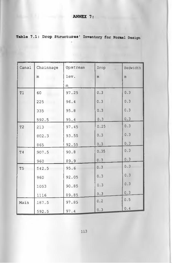
ANNEX 7
Table 7.1: Drop Structures' Inventory for Noraal Deiign
Canal Chainnage
m
Upstream
lev.
m
Drop
m
Bedwidth
m
T1 60 97.25 0.3 0.3
225 96.4 0.3 0.3
335 95.8 0.3 0.3
592.5 95.4 0.3 0.3
T2 213 97.45 0.25 0.3
802.3 93.55 0.3 0.3
865 92.55 0.3 0.3
T4 907.5 90.8 0.35 0.3
960 89.9 0.3 0.3
T5 542.5 95.6 0.3 0.3
960 92.05 0.3 0.3
1053 90.85 0.3 0.3
1116 89.85 0.3 0.3
Main 187.5 97.85 0.2 0.5
592.5 97.4 0.3 _ 0.4
113

Table 7.2: Survey Data Results from the Questionnaire
Output
(ha/day)
Grid (mxm) Time Taken for
Reduction of
Data
(hours/ha)
Time Taken in
Ploting and
Interpolating
Data
4 20x20 0.5 1
2 20x20 1 3
6 20x20 1 1.5
5 100x100 0.5 -
20 25x25 2 6
5 25x25 4 2
3 50x50 3 6
3 20x20 0.5 1
3 20x20 4 3
5 25x25 - ;
3 20x20 0.5 1
4 20x20 0.5 1
114

Table 7.3: Design Activities Ranking Resul*:
No: of responses per design activity.
d e f q h i j k2 2 4 1 1 12 0 0 3 3 2
115


su m m a ryfile: SLDlength of secondary (m ): length of tertiary (m ): 4<length of drain (m ): 3 64 .
num ber of rotation block num ber of ro tation subbl
P I < j u r « 7.2 c:»n«l and drain layout '

LEGEND
CM
0J*ooL.D
0
ooL—□
ground level
embankment level
x .a) X ,0) -*-< I—100.00.
99.00.1 2 3 A
X■*" X
98.00.4
>---------------------- 5 - 6 7 8 9 1 0
97.00.
96.00.
H--------------------------------------------- a11
DISCHARGE ( m 3 /s ) L J s u * y !____________________________i i 8 3 9 i S J I IS JCHAINAGE
i _ 3 i t i u _________________l 3 31 i i § i I 3ISGROUND LEVEL M L 11 1
5 S J 5____________________________3 22 ! \ $ s 355 iFULL SUPPLY LEVEL
i 1 1 18 1
...... . . . . 1 i 2 2j1 32 2l g a jBANK LEVEL I 15 11 I S ! 1 __ J 1 * 1 2l \ S K !BED LEVEL a is j i \ 1 L ______S J £ __________ 2L £ 2 5 «BED SLOPE
o|o oo o5 1 !§ §§ i
1I f ! 1
BED WIDTH s i § 23 i 83 1 ^ s __ i .is ___k . j Isss 3CUT/FILL (m 3 ) ' i $ ! _______ §__________ § L _____CUMUL C U T /F ILL 184,31 __i__!__1 1 _______ ___________ __ __________ L3L_
CANAL MAIN Scale fac to r 20.00
LONG SECTION SCALEvertical......... 1: 175holizontal..... 1: 3500
Figure 7.4 - Main Canal Profile
Ter
tiar
y o
ffta
ke
T3


LEGENDLDTi H* o <p (1)C ^D o O D +-> -+->
C ° o- § > • > % b! L Un •- •-O i- i_<D 0 a)
( / ) \— (—
ground Jevel
98.00-.
97.00_
96.00]
95.00_
9 f0 0 .
93.00.
92.00.
91-00-
90.00.
13 * 5 6 7 8 9
-
1112
1314
i
DISCHARGE ( m 3 / s ) 1 ii1 i I S§ ssi j lU j I S i i i sT _ ] L J S JS j L S 5CHAINAGE i___ SI\ L 31 i l l i L i i ___S1 3T 2L I \ J l Ji______ i L _ 1ground Level i 1i _j sL SiS | j 3 11 l5 \T i__________________ L i _ s ____jFULL SUPPLY LEVEL ! SIL _ J j 5 £I S3 J 33 3i 3T l a3 31 « I s IBANK LEVEL i SI\ 5 3 «SS 5j__ j 3 33 S 3T i . . 13 31 £ L i sBED LEVEL
i 31i % i 1 | SL_ J i ;S ! ! * l T i i_si $ s S lBED SLOPE 1 1! § 1 1!! _____ j |n s ! I
T! 1LJ! £ L ! !
BED WIDTH ) 3]s k sb SSSB 9S 38 S3 93 A ______ t 31 $ 3 35 9CUT/FILL (m 3 ) L !L 8 L !___ 3 1 \ 3 ! _ . j L l__ i L ___ 1CUMUL C U T/F ILL: - 2 4 .4 6 r if «1 13 I 1 L 5 i . - i _ J ____k 1_______ \_____
CANAL T3 LONG SECTION Scale fa c to r 20 .00
Figure 7.7 — Canal T3 Profile
verhoi
SCALEtica l..........1:izontal......1:
175 : 3500

U N P
in ro0 4 , 0;O O oo
t S iT Y O F N A I R O B I L ) B R A R '
LEGEND
CANAL T4 Scale fa c to r 20.00
LONG SECTION
Figure 7.8 — Canal T4 Profile.
SCALEvertical........1: 200holizontal....1: 4000

CANAL T5 LONG SECTIONScale fa c to r 20.00
Figure 7.9 — Canal T5 Canal
SCALEvertical.........1* 225holizontal..... 1- 4500
----- I—-------

NORMAL DESIGN FOR MAIN CA NAl


■


