Immersive, highly realistic in-lab experiments of cycling route choices

Center for Transportation, Environment, and Community Health Final Report

by Ricardo A Daziano, So-Yeon Yoon, Tomás Rossetti

June 29, 2021

DISCLAIMER The contents of this report reflect the views of the authors, who are responsible for the facts and the accuracy of the information presented herein. This document is disseminated in the interest of information exchange. The report is funded, partially or entirely, by a grant from the U.S. Department of Transportation’s University Transportation Centers Program. However, the U.S. Government assumes no liability for the contents or use thereof.

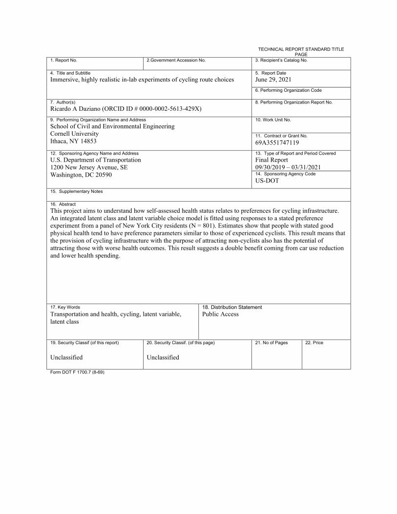
TECHNICAL REPORT STANDARD TITLE PAGE

1. Report No. 2.Government Accession No. 3. Recipient’s Catalog No. 4. Title and Subtitle 5. Report Date Immersive, highly realistic in-lab experiments of cycling route choices

June 29, 2021 6. Performing Organization Code

7. Author(s) 8. Performing Organization Report No. Ricardo A Daziano (ORCID ID # 0000-0002-5613-429X)

9. Performing Organization Name and Address 10. Work Unit No. School of Civil and Environmental Engineering Cornell University Ithaca, NY 14853

11. Contract or Grant No. 69A3551747119

12. Sponsoring Agency Name and Address 13. Type of Report and Period Covered U.S. Department of Transportation 1200 New Jersey Avenue, SE Washington, DC 20590

Final Report 09/30/2019 – 03/31/2021 14. Sponsoring Agency Code US-DOT

15. Supplementary Notes 16. Abstract This project aims to understand how self-assessed health status relates to preferences for cycling infrastructure. An integrated latent class and latent variable choice model is fitted using responses to a stated preference experiment from a panel of New York City residents (N = 801). Estimates show that people with stated good physical health tend to have preference parameters similar to those of experienced cyclists. This result means that the provision of cycling infrastructure with the purpose of attracting non-cyclists also has the potential of attracting those with worse health outcomes. This result suggests a double benefit coming from car use reduction and lower health spending.

17. Key Words 18. Distribution Statement Transportation and health, cycling, latent variable, latent class

Public Access

19. Security Classif (of this report) 20. Security Classif. (of this page) 21. No of Pages 22. Price

Unclassified Unclassified

Form DOT F 1700.7 (8-69)

Immersive, highly realistic in-lab experiments of cycling route choices

Abstract

This project aims to understand how self-assessed health status relates to preferences for cycling in-

frastructure. An integrated latent class and latent variable choice model is fitted using responses to a

stated preference experiment from a panel of New York City residents (N = 801). Estimates show that

people with stated good physical health tend to have preference parameters similar to those of experi-

enced cyclists. This result means that the provision of cycling infrastructure with the purpose of at-

tracting non-cyclists also has the potential of attracting those with worse health outcomes. This result

suggests a double benefit coming from car use reduction and lower health spending.

Keywords: Transportation and health, cycling, latent variable, latent class

Introduction

The past two decades have seen increasing research interest in the analysis of cyclists’

preferences for cycling infrastructure [1, 2]. These studies have used different methods to

identify the built environment characteristics that are preferred by cyclists, and that could

therefore be exploited to encourage a broader modal shift toward sustainable transportation. The

vast consensus is that cyclists prefer infrastructure that is separated from traffic, as well as

shorter and more direct routes [3].

Even though this consensus may be true for the population as a whole, there are significant

differences both within cyclists and non-cyclists that should be considered during policy

formulation. For example, a review carried out by Aldred et al. [4] shows that women and the

elderly tend to have a stronger preference for segregated cycling paths. Another distinction that

has been identified in the literature has to do with cycling experience. People that have less

cycling experience also tend to have a stronger preference for segregation from motorized

vehicles [5, 6]. This information can be used by city planners to tailor their policies to the needs

of different segments of the population.

The relationship between health and cycling has also been heavily studied, but unfortunately not

from the point of view of infrastructure provision or preferences. The research questions relating

the two have primarily focused on the effects cycling has on people’s health. As expected,

previous research has concluded that, on average, cyclists have a lower prevalence of diabetes,

hypercholesterolemia, and obesity [7, 8]. Understanding the interconnection of cycling

preferences and health could lead to infrastructure that is better suited to the less healthy segment

of the population, motivating this segment to start cycling and improve their health outcomes.

In this study, we address the relationship between self-assessed health status and infrastructure

preferences. We do this using data collected from an online survey of New York City residents.

We then use this data to estimate a latent class and latent variable choice model that describe

health outcomes and cycling experience. Results show that respondents with higher body mass

indices (BMI) and worse self-assessed health status have a stronger preference for segregated

infrastructure and a lower sensitivity toward travel time.

The rest of the report is organized as follows: The data collection process is described first, with

a description of the sample. Then, the latent class and latent variable methodology is presented.

After this, results are shown and discussed.

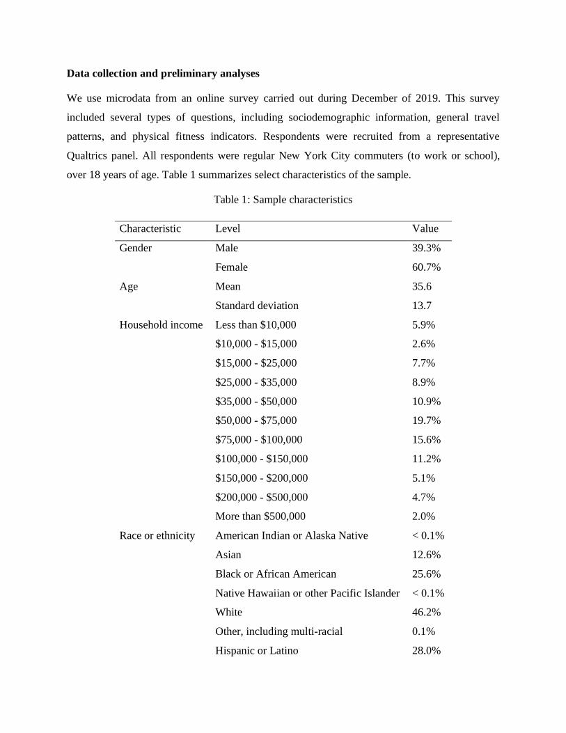
Data collection and preliminary analyses

We use microdata from an online survey carried out during December of 2019. This survey

included several types of questions, including sociodemographic information, general travel

patterns, and physical fitness indicators. Respondents were recruited from a representative

Qualtrics panel. All respondents were regular New York City commuters (to work or school),

over 18 years of age. Table 1 summarizes select characteristics of the sample.

Table 1: Sample characteristics

Characteristic Level Value

Gender Male 39.3%

Female 60.7%

Age Mean 35.6

Standard deviation 13.7

Household income Less than $10,000 5.9%

$10,000 - $15,000 2.6%

$15,000 - $25,000 7.7%

$25,000 - $35,000 8.9%

$35,000 - $50,000 10.9%

$50,000 - $75,000 19.7%

$75,000 - $100,000 15.6%

$100,000 - $150,000 11.2%

$150,000 - $200,000 5.1%

$200,000 - $500,000 4.7%

More than $500,000 2.0%

Race or ethnicity American Indian or Alaska Native < 0.1%

Asian 12.6%

Black or African American 25.6%

Native Hawaiian or other Pacific Islander < 0.1%

White 46.2%

Other, including multi-racial 0.1%

Hispanic or Latino 28.0%

Characteristic Level Value

Cars available None 34.7%

One 47.4%

Two 14.6%

Three or more 3.2%

Home location Bronx 15.2%

Brooklyn 25.0%

Manhattan 35.6%

Queens 22.3%

Staten Island 1.9%

BMI Mean 25.3

Standard deviation 5.9

Obese (BMI > 30) 18.7%

Overweight (25 BMI < 30) 26.8%

Healthy (18:5 BMI < 25) 53.8%

Underweight (BMI < 18:5) 0.7%

The section of the survey that is most relevant to this study is a set of choice experiments

regarding route choice using public bicycles. Each respondent faced seven binary choice

scenarios, where two hypothetical routes were shown. The scenarios were developed in a virtual

city environment similar to a typical Manhattan avenue. Examples of the virtual cycling

conditions are shown in Figure 1, and the experimental attributes with their levels are shown in

Table 2. A total of 5,560 choices were recorded.

Table 2: Attribute levels of choice scenarios

Variable Levels

Travel time Pivoted around respondents’ stated travel time.

Traffic / Speed Heavy traffic and slow speeds, or normal traffic flow with high speeds. This relationship

was designed to replicate a slow, congested street, or an uncongested street with cars

driving at the speed limit.

One or two way lane Either one or two-way cycle lanes.

Parking Inexistent, on left or on right.

Lane design Painted surface and/or with a buffer between the lane and cars. All choice scenarios had

at least one of these possible protections.

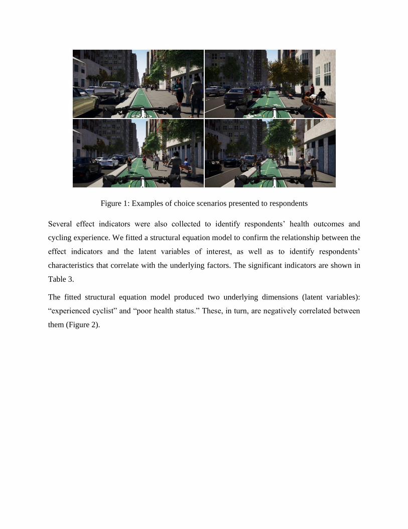
Figure 1: Examples of choice scenarios presented to respondents

Several effect indicators were also collected to identify respondents’ health outcomes and

cycling experience. We fitted a structural equation model to confirm the relationship between the

effect indicators and the latent variables of interest, as well as to identify respondents’

characteristics that correlate with the underlying factors. The significant indicators are shown in

Table 3.

The fitted structural equation model produced two underlying dimensions (latent variables):

“experienced cyclist” and “poor health status.” These, in turn, are negatively correlated between

them (Figure 2).

Table 3: Indicators used to fit a latent variable model using structural equation modeling

Indicator Type of response

Health outcomes

Body Mass Index (BMI) Continuous. Constructed using stated height and weight.

Self-reported health status 5 point Likert scale, from “Excellent” to “Very poor.”

Cycling experience

Self-description of type of cyclist 4 point ordinal response, from “An advanced, confident

cyclist who is comfortable riding in most traffic

situations” to “I do not know how to bike.”

Uses app to access Citi Bike Binary

Bikes at least once a week

during the fall or spring (two

indicators)

Binary

Typically walks or bikes during a

weekday or weekend for more than

10 minutes (two indicators)

Binary

Figure 2: Relation between the two latent variables produced by the structural equation model, at

the respondent level

Methodology

To identify how preference structures vary across respondents depending on their general health

outcome, we use an integrated choice and latent class model. Nevertheless, because these health

outcomes are not directly measurable using an online survey, we model them using latent

variables. This produces an integrated choice, latent class and latent variable model. Each one of

these components, as well as their integration, is described in the following subsections.

Latent class choice models

One strategy for modeling unobserved heterogeneity in preferences is to assume a discrete

distribution of preferences, representing a discrete number of consumer categories of classes.

Econometrically, the underlying categories may be inferred by estimating latent classes, as

proposed by Kamakura and Russell [9]. Latent class choice models include two components: one

relates individuals to the latent (unobserved) classes, whereas the other relates individuals to

choices given their latent class.

The utility derived by individual j when they choose alternative i given that they belong to

class s can be represented by (1). Xij is a vector of observed alternative attributes and consumer

characteristics, and βs is a vector of class-specific taste parameters. Utility Uijs can take different

forms across classes, including varying distributional assumptions for the class-specific error

component, εijs, and the specification of the indirect utility function, V s.

𝑈𝑖𝑗𝑠 = 𝑉𝑠(𝑿𝑖𝑗; 𝜷𝑠) + 𝜀𝑖𝑗

𝑠 (1)

If we assume, first, a random utility maximization framework and, second, that εs are

independent and identically distributed Extreme Value Type I, then the probability

that j chooses i given that they belong to class sis equal to the conditional logit choice probability

(2). Cjs is the choice set individual j faces given that they belong to class s in this equation.

If V s is assumed to have a linear specification, as is usually done in the literature, the scale

parameter μs has to be normalized to ensure parameter identification.

𝑃𝑗(𝑖|𝑠, 𝑿𝑖𝑗; 𝜷𝑠) =exp (𝜇𝑠𝑉𝑠(𝑿𝑖𝑗; 𝜷𝑠))

∑ exp (𝜇𝑠𝑉𝑠(𝑿𝑙𝑗; 𝜷𝑠))𝑙∈𝐶𝑗𝑠

(2)

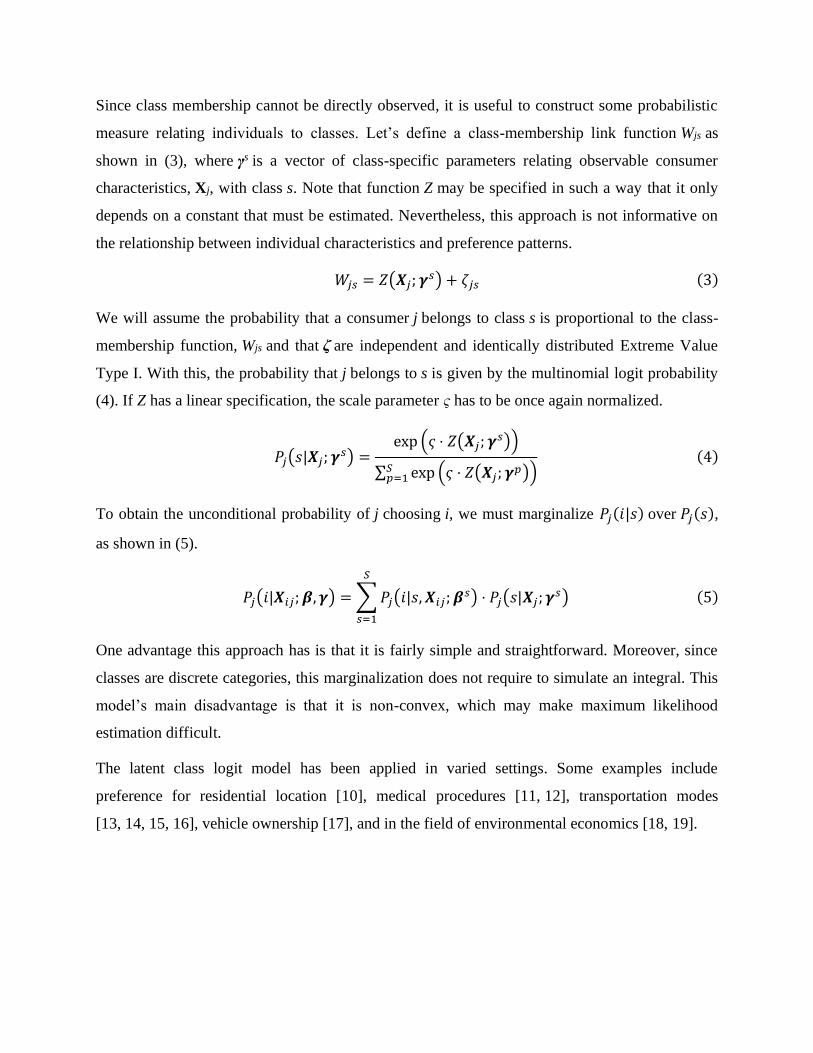
Since class membership cannot be directly observed, it is useful to construct some probabilistic

measure relating individuals to classes. Let’s define a class-membership link function Wjs as

shown in (3), where γs is a vector of class-specific parameters relating observable consumer

characteristics, Xj, with class s. Note that function Z may be specified in such a way that it only

depends on a constant that must be estimated. Nevertheless, this approach is not informative on

the relationship between individual characteristics and preference patterns.

𝑊𝑗𝑠 = 𝑍(𝑿𝑗; 𝜸𝑠) + 𝜁𝑗𝑠 (3)

We will assume the probability that a consumer j belongs to class s is proportional to the class-

membership function, Wjs and that ζ are independent and identically distributed Extreme Value

Type I. With this, the probability that j belongs to s is given by the multinomial logit probability

(4). If Z has a linear specification, the scale parameter ς has to be once again normalized.

𝑃𝑗(𝑠|𝑿𝑗; 𝜸𝑠) =exp (𝜍 ⋅ 𝑍(𝑿𝑗; 𝜸𝑠))

∑ exp (𝜍 ⋅ 𝑍(𝑿𝑗; 𝜸𝑝))𝑆𝑝=1

(4)

To obtain the unconditional probability of j choosing i, we must marginalize 𝑃𝑗(𝑖|𝑠) over 𝑃𝑗(𝑠),

as shown in (5).

𝑃𝑗(𝑖|𝑿𝑖𝑗; 𝜷, 𝜸) = ∑ 𝑃𝑗(𝑖|𝑠, 𝑿𝑖𝑗; 𝜷𝑠) ⋅ 𝑃𝑗(𝑠|𝑿𝑗; 𝜸𝑠)

𝑆

𝑠=1

(5)

One advantage this approach has is that it is fairly simple and straightforward. Moreover, since

classes are discrete categories, this marginalization does not require to simulate an integral. This

model’s main disadvantage is that it is non-convex, which may make maximum likelihood

estimation difficult.

The latent class logit model has been applied in varied settings. Some examples include

preference for residential location [10], medical procedures [11, 12], transportation modes

[13, 14, 15, 16], vehicle ownership [17], and in the field of environmental economics [18, 19].

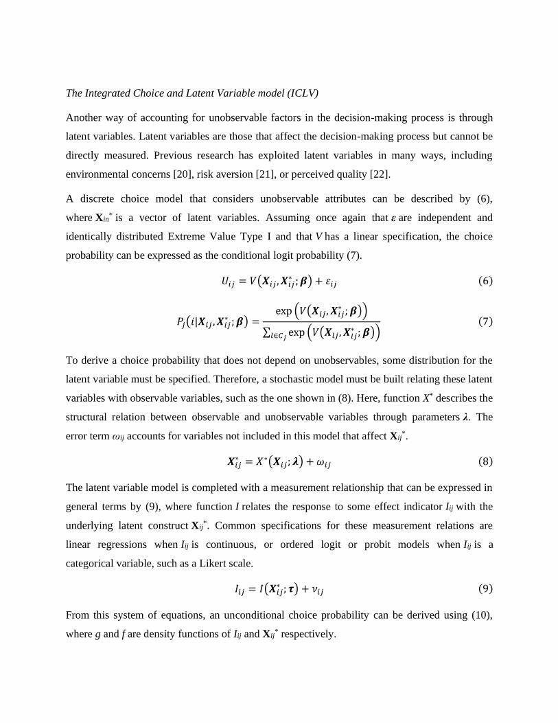
The Integrated Choice and Latent Variable model (ICLV)

Another way of accounting for unobservable factors in the decision-making process is through

latent variables. Latent variables are those that affect the decision-making process but cannot be

directly measured. Previous research has exploited latent variables in many ways, including

environmental concerns [20], risk aversion [21], or perceived quality [22].

A discrete choice model that considers unobservable attributes can be described by (6),

where Xin* is a vector of latent variables. Assuming once again that ε are independent and

identically distributed Extreme Value Type I and that V has a linear specification, the choice

probability can be expressed as the conditional logit probability (7).

𝑈𝑖𝑗 = 𝑉(𝑿𝑖𝑗 , 𝑿𝑖𝑗∗ ; 𝜷) + 𝜀𝑖𝑗 (6)

𝑃𝑗(𝑖|𝑿𝑖𝑗 , 𝑿𝑖𝑗∗ ; 𝜷) =

exp (𝑉(𝑿𝑖𝑗 , 𝑿𝑖𝑗∗ ; 𝜷))

∑ exp (𝑉(𝑿𝑙𝑗 , 𝑿𝑙𝑗∗ ; 𝜷))𝑙∈𝐶𝑗

(7)

To derive a choice probability that does not depend on unobservables, some distribution for the

latent variable must be specified. Therefore, a stochastic model must be built relating these latent

variables with observable variables, such as the one shown in (8). Here, function X* describes the

structural relation between observable and unobservable variables through parameters λ. The

error term ωij accounts for variables not included in this model that affect Xij*.

𝑿𝑖𝑗∗ = 𝑋∗(𝑿𝑖𝑗; 𝝀) + 𝜔𝑖𝑗 (8)

The latent variable model is completed with a measurement relationship that can be expressed in

general terms by (9), where function I relates the response to some effect indicator Iij with the

underlying latent construct Xij*. Common specifications for these measurement relations are

linear regressions when Iij is continuous, or ordered logit or probit models when Iij is a

categorical variable, such as a Likert scale.

𝐼𝑖𝑗 = 𝐼(𝑿𝑖𝑗∗ ; 𝝉) + 𝜈𝑖𝑗 (9)

From this system of equations, an unconditional choice probability can be derived using (10),

where g and f are density functions of Iij and Xij* respectively.

𝑃𝑗(𝑖|𝑿𝑖𝑗 , 𝐼𝑖𝑗; 𝜷, 𝝉, 𝝀) = ∫ 𝑃𝑗(𝑖|𝑿𝑖𝑗 , 𝑿𝑖𝑗∗ ; 𝜷) ⋅ 𝑔(𝐼𝑖𝑗|𝑿𝑖𝑗

∗ ; 𝝉) ⋅ 𝑓(𝑿𝑖𝑗∗ ; 𝝀) 𝑑𝑿𝑖𝑗 (10)

This Integrated Choice and Latent Variable model (ICLV) was proposed by Walker and Ben-

Akiva [23] and has gained wide popularity in the choice modeling community, despite some

criticisms. Even though most applications involve attitudinal latent variables (those that are

related to some unobservable characteristic of consumers), perceptual latent variables can also be

constructed Bahamonde-Birke et al. [24].

A latent class logit model with latent variables

An empirical problem of latent class choice models is that there is no clear interpretation of the

fitted latent segments. What researchers usually do is to make intuitive sense of the overall

segment by looking at the observable variables correlated with class membership model. These

interpretations are hypotheses and not conclusions founded on the econometric model itself. If

attitudinal latent variables are used to construct the class-membership model, direct and

empirically well-founded relationships between latent constructs and class-specific taste

parameters can be derived. This approach also frees the researcher from subjective

interpretations of the parameters.

A latent class logit model with latent variables can be constructed by defining the class-

membership function solely based on latent variables, as in (11). This model produces a class-

membership and choice probabilities conditional on these latent variables, shown in (12) and

(13).

𝑊𝑗𝑠 = 𝑍(𝑿𝑗∗; 𝜸𝑠) + 𝜁𝑗𝑠 (11)

𝑃𝑗(𝑠|𝑿𝑗∗; 𝜸𝑠) =

exp (𝜍 ⋅ 𝑍(𝑿𝑗∗; 𝜸𝑠))

∑ exp (𝜍 ⋅ 𝑍(𝑿𝑗∗; 𝜸𝑝))𝑆

𝑝=1

(12)

𝑃𝑗(𝑖|𝑿𝑖𝑗 , 𝑿𝑗∗; 𝜷, 𝜸) = ∑ 𝑃𝑗(𝑖|𝑠, 𝑿𝑖𝑗; 𝜷𝑠) ⋅ 𝑃𝑗(𝑠|𝑿𝑗

∗; 𝜸𝑠)

𝑆

𝑠=1

(13)

From the system of equations, we can obtain an unconditional choice probability that can be used

to make inference, as shown in (14).

𝑃𝑗(𝑖|𝑿𝑖𝑗 , 𝐼𝑖𝑗 ; 𝜷, 𝝉, 𝝀, 𝜸) = ∫ (∑ 𝑃𝑗(𝑖|𝑠, 𝑿𝑖𝑗; 𝜷𝑠) ⋅ 𝑃𝑗(𝑠|𝑿𝑗∗; 𝜸𝑠)

𝑆

𝑠=1

) ⋅ 𝑔(𝐼𝑖𝑗|𝑿𝑗∗; 𝝉) ⋅ 𝑓(𝑿𝑖𝑗

∗ ; 𝝀) 𝑑𝑿𝑗∗(14)

Model parameters can be obtained using maximum likelihood estimation. Assuming that there

are a total of N respondents and that each respondent n observed Tj choice scenarios, the

likelihood can be expressed as:

ℒ(𝜷, 𝝉, 𝝀, 𝜸|𝑿) = ∏ ∫ ∏ 𝑃𝑗(𝑖|𝑿𝑖𝑗𝑡 , 𝑿𝑗∗; 𝜷, 𝜸)

𝑇𝑗

𝑡=1

⋅ 𝑔(𝐼𝑖𝑗|𝑿𝑗∗; 𝝉) ⋅ 𝑓(𝑿𝑗

∗; 𝝀) 𝑑𝑿𝑗∗

𝐽

𝑗=1

(15)

There are a few examples of this model being used in the literature, including Hess et al. [20] and

Krueger et al. [25].

Results

The following subsections discuss the results of modeling the data presented in a previous

section using the latent class and latent variable method. We will first discuss direct estimates,

and then analyze marginal rates of substitution of the two models obtained. All results shown

were obtained using the Apollo package in R [26].

This section presents results for two latent class and latent variable models. The one that

addresses this study’s research question uses a latent variable describing health status to

infrastructure preference. The second one relates cycling experience to these preferences. This

model was estimated to compare and validate the results of the first one. Note that because these

two latent variables are highly correlated (see Figure 2), both could not be integrated into a

single model. Finally, a standard conditional logit was also estimated to have a baseline

comparison for parameter estimates, marginal rates of substitution, and goodness-of-fit

measures. Table 4 shows the results for all models.

First, the likelihood values at convergence of the choice components for the latent class and

latent variable models are higher than the one for the baseline MNL model. On the one hand, this

result means that there is significant preference heterogeneity that cannot be captured by the

conditional logit. On the other hand, the choice likelihood of Model 1 is slightly higher than the

one of Model 2. Nevertheless, these differences are small.

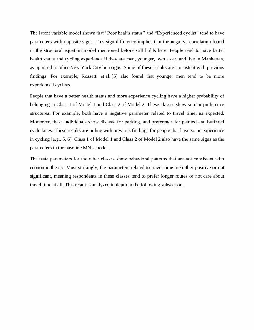
The latent variable model shows that “Poor health status” and “Experienced cyclist” tend to have

parameters with opposite signs. This sign difference implies that the negative correlation found

in the structural equation model mentioned before still holds here. People tend to have better

health status and cycling experience if they are men, younger, own a car, and live in Manhattan,

as opposed to other New York City boroughs. Some of these results are consistent with previous

findings. For example, Rossetti et al. [5] also found that younger men tend to be more

experienced cyclists.

People that have a better health status and more experience cycling have a higher probability of

belonging to Class 1 of Model 1 and Class 2 of Model 2. These classes show similar preference

structures. For example, both have a negative parameter related to travel time, as expected.

Moreover, these individuals show distaste for parking, and preference for painted and buffered

cycle lanes. These results are in line with previous findings for people that have some experience

in cycling [e.g., 5, 6]. Class 1 of Model 1 and Class 2 of Model 2 also have the same signs as the

parameters in the baseline MNL model.

The taste parameters for the other classes show behavioral patterns that are not consistent with

economic theory. Most strikingly, the parameters related to travel time are either positive or not

significant, meaning respondents in these classes tend to prefer longer routes or not care about

travel time at all. This result is analyzed in depth in the following subsection.

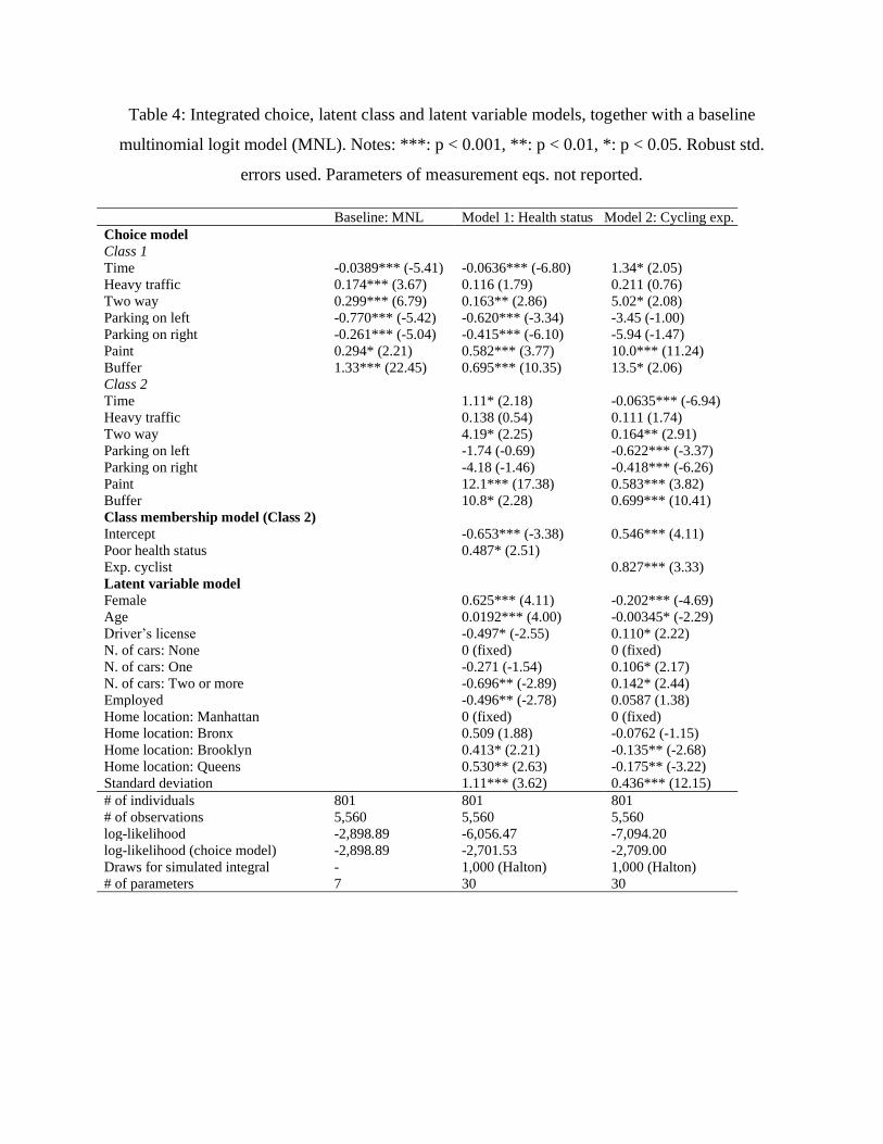
Table 4: Integrated choice, latent class and latent variable models, together with a baseline

multinomial logit model (MNL). Notes: ***: p < 0.001, **: p < 0.01, *: p < 0.05. Robust std.

errors used. Parameters of measurement eqs. not reported.

Baseline: MNL Model 1: Health status Model 2: Cycling exp.

Choice model Class 1 Time -0.0389*** (-5.41) -0.0636*** (-6.80) 1.34* (2.05)

Heavy traffic 0.174*** (3.67) 0.116 (1.79) 0.211 (0.76)

Two way 0.299*** (6.79) 0.163** (2.86) 5.02* (2.08)

Parking on left -0.770*** (-5.42) -0.620*** (-3.34) -3.45 (-1.00)

Parking on right -0.261*** (-5.04) -0.415*** (-6.10) -5.94 (-1.47)

Paint 0.294* (2.21) 0.582*** (3.77) 10.0*** (11.24)

Buffer 1.33*** (22.45) 0.695*** (10.35) 13.5* (2.06)

Class 2 Time 1.11* (2.18) -0.0635*** (-6.94)

Heavy traffic 0.138 (0.54) 0.111 (1.74)

Two way 4.19* (2.25) 0.164** (2.91)

Parking on left -1.74 (-0.69) -0.622*** (-3.37)

Parking on right -4.18 (-1.46) -0.418*** (-6.26)

Paint 12.1*** (17.38) 0.583*** (3.82)

Buffer 10.8* (2.28) 0.699*** (10.41)

Class membership model (Class 2) Intercept -0.653*** (-3.38) 0.546*** (4.11)

Poor health status 0.487* (2.51) Exp. cyclist 0.827*** (3.33)

Latent variable model Female 0.625*** (4.11) -0.202*** (-4.69)

Age 0.0192*** (4.00) -0.00345* (-2.29)

Driver’s license -0.497* (-2.55) 0.110* (2.22)

N. of cars: None 0 (fixed) 0 (fixed)

N. of cars: One -0.271 (-1.54) 0.106* (2.17)

N. of cars: Two or more -0.696** (-2.89) 0.142* (2.44)

Employed -0.496** (-2.78) 0.0587 (1.38)

Home location: Manhattan 0 (fixed) 0 (fixed)

Home location: Bronx 0.509 (1.88) -0.0762 (-1.15)

Home location: Brooklyn 0.413* (2.21) -0.135** (-2.68)

Home location: Queens 0.530** (2.63) -0.175** (-3.22)

Standard deviation 1.11*** (3.62) 0.436*** (12.15)

# of individuals 801 801 801

# of observations 5,560 5,560 5,560

log-likelihood -2,898.89 -6,056.47 -7,094.20

log-likelihood (choice model) -2,898.89 -2,701.53 -2,709.00

Draws for simulated integral - 1,000 (Halton) 1,000 (Halton)

# of parameters 7 30 30

Marginal rates of substitution

The ideal bicycle lane design has been a matter of debate among urban designers. City planners

usually have to deal with the trade-off between segregation from cars (something the literature

has consistently demonstrated is desirable for cyclists) and cost. Whereas cheaper bicycle lanes

allow to expand the network at a faster pace, this cheaper infrastructure can fail to attract or even

deter new riders. Given this dichotomy, the marginal rate of substitution (MRS) between

different kinds of designs and travel time can help assess the costs and social benefits of different

approaches to cycling infrastructure provision.

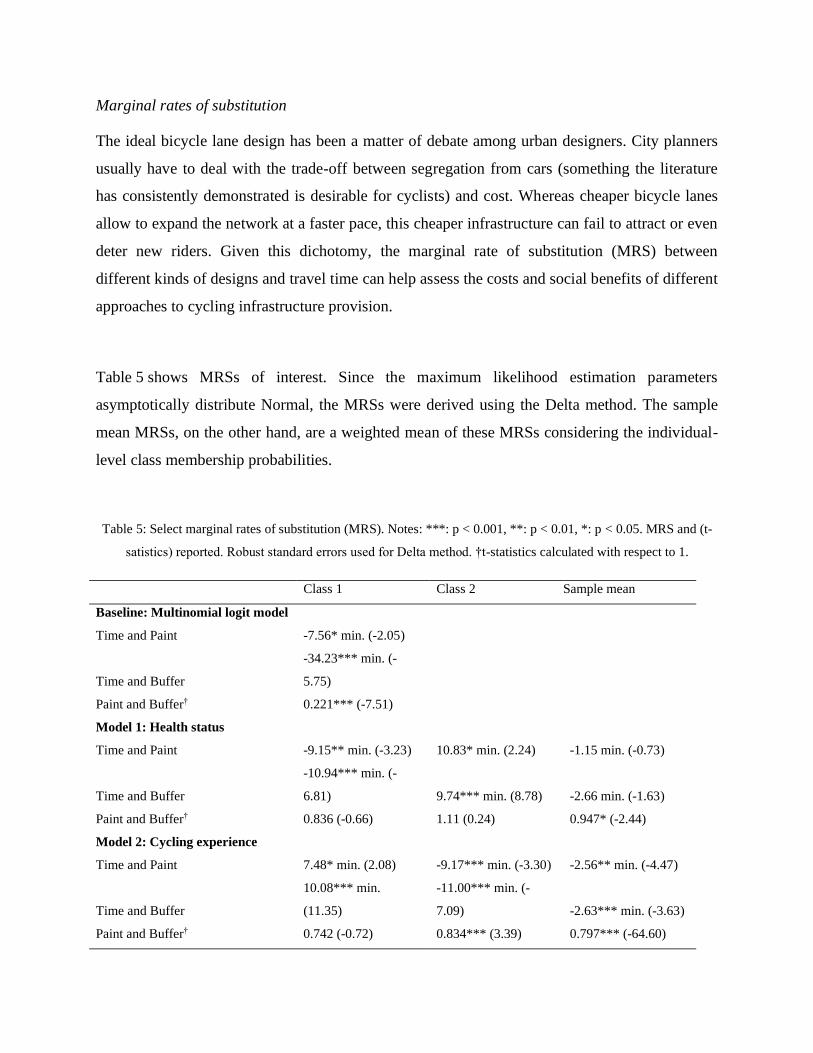
Table 5 shows MRSs of interest. Since the maximum likelihood estimation parameters

asymptotically distribute Normal, the MRSs were derived using the Delta method. The sample

mean MRSs, on the other hand, are a weighted mean of these MRSs considering the individual-

level class membership probabilities.

Table 5: Select marginal rates of substitution (MRS). Notes: ***: p < 0.001, **: p < 0.01, *: p < 0.05. MRS and (t-

satistics) reported. Robust standard errors used for Delta method. †t-statistics calculated with respect to 1.

Class 1 Class 2 Sample mean

Baseline: Multinomial logit model

Time and Paint -7.56* min. (-2.05)

Time and Buffer

-34.23*** min. (-

5.75)

Paint and Buffer† 0.221*** (-7.51)

Model 1: Health status

Time and Paint -9.15** min. (-3.23) 10.83* min. (2.24) -1.15 min. (-0.73)

Time and Buffer

-10.94*** min. (-

6.81) 9.74*** min. (8.78) -2.66 min. (-1.63)

Paint and Buffer† 0.836 (-0.66) 1.11 (0.24) 0.947* (-2.44)

Model 2: Cycling experience

Time and Paint 7.48* min. (2.08) -9.17*** min. (-3.30) -2.56** min. (-4.47)

Time and Buffer

10.08*** min.

(11.35)

-11.00*** min. (-

7.09) -2.63*** min. (-3.63)

Paint and Buffer† 0.742 (-0.72) 0.834*** (3.39) 0.797*** (-64.60)

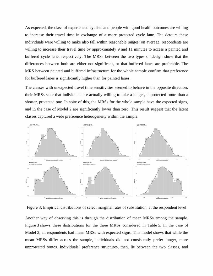
As expected, the class of experienced cyclists and people with good health outcomes are willing

to increase their travel time in exchange of a more protected cycle lane. The detours these

individuals were willing to make also fall within reasonable ranges: on average, respondents are

willing to increase their travel time by approximately 9 and 11 minutes to access a painted and

buffered cycle lane, respectively. The MRSs between the two types of design show that the

differences between both are either not significant, or that buffered lanes are preferable. The

MRS between painted and buffered infrastructure for the whole sample confirm that preference

for buffered lanes is significantly higher than for painted lanes.

The classes with unexpected travel time sensitivities seemed to behave in the opposite direction:

their MRSs state that individuals are actually willing to take a longer, unprotected route than a

shorter, protected one. In spite of this, the MRSs for the whole sample have the expected signs,

and in the case of Model 2 are significantly lower than zero. This result suggest that the latent

classes captured a wide preference heterogeneity within the sample.

Figure 3: Empirical distributions of select marginal rates of substitution, at the respondent level

Another way of observing this is through the distribution of mean MRSs among the sample.

Figure 3 shows these distributions for the three MRSs considered in Table 5. In the case of

Model 2, all respondents had mean MRSs with expected signs. This model shows that while the

mean MRSs differ across the sample, individuals did not consistently prefer longer, more

unprotected routes. Individuals’ preference structures, then, lie between the two classes, and

cannot be described by only one. This is also shown in Figure 4, where it can be observed that

respondents’ class membership probabilities lie within mid-range values.

Figure 4: Empirical distributions of class-membership probabilities

Something different happened in the case of Model 1, where the mean MRSs are more spread

out. This result may be a consequence of the larger variance in the class-membership component

of Model 1. This produces more weakly identified class membership probabilities. Nevertheless,

these values could show there are other underlying issues with the dataset. For example, people

with worse health status may not experience cycling often, and therefore cannot consider the

attributes adequately. Another issue could be that the latent variable and latent classes are weakly

identified, and therefore cannot capture respondents’ underlying heterogeneity correctly.

Even though the MRSs for the conditional logit model have expected signs, their magnitudes

differ from the sample means in the random parameter logit models. This difference in

magnitude is likely coming from the conditional logit model not being able to recover

heterogeneity in preferences.

Conclusions

Previous research dedicated to identifying preferences for cycling infrastructure has failed to

consider the relationships of those preferences with health status. Understanding this association

is essential for policymakers to improve health outcomes from the low-impact physical exercise

that comes from cycling. If the specific needs of those with poorer health outcomes are addressed

in the infrastructure design process, there is a higher likelihood that they will engage in active

transportation and improve their health.

We used a stated preference data set from New York City to fit an integrated choice, latent class

and latent variable model to identify the relations between health and infrastructure preference.

Results show that people with lower health outcomes tend to be less sensitive to travel time and

more sensitive to protection from motorized vehicles. This preference structure is also very

similar to the one of inexperienced cyclists.

This study provides evidence that supports a double benefit from policies that promote cycling

among the inexperienced: these not only have the potential benefit of producing a shift towards

more sustainable modes of transportation, but also promote more physical exercise among the

population that is less physically fit. This double benefit has the potential to reduce public health

spending, as well as to decrease future spending to counter the effects of climate change.

References

[1] Nello-Deakin, S., Environmental determinants of cycling: Not seeing the forest for the

trees? Journal of Transport Geography, Vol. 85, No. November 2019, 2020, p. 102704.

[2] Pucher, J. and R. Buehler, Making cycling irresistible: Lessons from the Netherlands,

Denmark and Germany. Transport Reviews, Vol. 28, No. 4, 2008, pp. 495–528.

[3] Buehler, R. and J. Dill, Bikeway Networks: A Review of Effects on Cycling. Transport

Reviews, Vol. 36, No. 1, 2016, pp. 9–27.

[4] Aldred, R., B. Elliott, J. Woodcock, and A. Goodman, Cycling provision separated from

motor traffic: A systematic review exploring whether stated preferences vary by gender

and age. Transport Reviews, Vol. 1647, No. July, 2016, pp. 1–27.

[5] Rossetti, T., C. A. Guevara, P. Galilea, and R. Hurtubia, Modeling safety as a perceptual

latent variable to assess cycling infrastructure. Transportation Research Part A: Policy

and Practice, Vol. 111, No. February, 2018, pp. 252–265.

[6] Stinson, M. A. and C. R. Bhat, A comparison of the route preferences of experienced and

inexperienced bicycle commuters. Transportation Research Board 84th Annual

Meeting, , No. 512, 2005.

[7] Riiser, A., A. Solbraa, A. K. Jenum, K. I. Birkeland, and L. B. Andersen, Cycling and

walking for transport and their associations with diabetes and risk factors for

cardiovascular disease. Journal of Transport and Health, Vol. 11, No. December 2017,

2018, pp. 193–201.

[8] Lindström, M., Means of transportation to work and overweight and obesity: A population-

based study in southern Sweden. Preventive Medicine, Vol. 46, No. 1, 2008, pp. 22–28.

[9] Kamakura, W. and G. Russell, A Probabilistic Choice Model for Market Segmentation and

Elasticity Structure. Journal of Marketing Research, Vol. 26, No. 4, 1989, pp. 379–390.

[10] Walker, J. and J. Li, Latent lifestyle preferences and household location decisions. Journal

of Geographical Systems, Vol. 9, 2007, pp. 77–101.

[11] Ho, K. A., M. Acar, A. Puig, G. Hutas, and S. Fifer, What do Australian patients with

inflammatory arthritis value in treatment? A discrete choice experiment. Clinical

Rheumatology, Vol. 39, No. 4, 2020, pp. 1077–1089.

[12] Rozier, M. D., A. A. Ghaferi, A. Rose, N. J. Simon, N. Birkmeyer, and L. A. Prosser,

Patient Preferences for Bariatric Surgery: Findings from a Survey Using Discrete

Choice Experiment Methodology. JAMA Surgery, Vol. 154, No. 1, 2019, pp. 1–10.

[13] El Zarwi, F., A. Vij, and J. L. Walker, A discrete choice framework for modeling and

forecasting the adoption and diffusion of new transportation services. Transportation

Research Part C: Emerging Technologies, Vol. 79, 2017, pp. 207–223.

[14] Hurtubia, R., M. H. Nguyen, A. Glerum, and M. Bierlaire, Integrating psychometric

indicators in latent class choice models. Transportation Research Part A: Policy and

Practice, Vol. 64, 2014, pp. 135–146.

[15] Shen, J., Latent class model or mixed logit model? A comparison by transport mode

choice data. Applied Economics, Vol. 41, No. 22, 2009, pp. 2915–2924.

[16] Bhat, C. R., An Endogenous Segmentation Mode Choice Model with an Application to

Intercity Travel. Transportation Science, Vol. 31, No. 1, 1997, pp. 34–48.

[17] Ferguson, M., M. Mohamed, C. D. Higgins, E. Abotalebi, and P. Kanaroglou, How open

are Canadian households to electric vehicles? A national latent class choice analysis

with willingness-to-pay and metropolitan characterization. Transportation Research

Part D: Transport and Environment, Vol. 58, No. December 2017, 2018, pp. 208–224.

[18] Araghi, Y., M. Kroesen, E. Molin, and B. Van Wee, Revealing heterogeneity in air

travelers’ responses to passenger-oriented environmental policies: A discrete-choice

latent class model. International Journal of Sustainable Transportation, Vol. 10, No. 9,

2016, pp. 765–772.

[19] Beharry-Borg, N. and R. Scarpa, Valuing quality changes in Caribbean coastal waters for

heterogeneous beach visitors. Ecological Economics, Vol. 69, No. 5, 2010, pp. 1124–

1139.

[20] Hess, S., J. Shires, and A. Jopson, Accommodating underlying pro-environmental

attitudes in a rail travel context: Application of a latent variable latent class

specification. Transportation Research Part D:Transport and Environment, Vol. 25,

2013, pp. 42–48.

[21] Tsirimpa, A., A. Polydoropoulou, and C. Antoniou, Development of a latent variable

model to capture the impact of risk aversion on travelers’ switching behavior. Journal of

Choice Modelling, Vol. 3, No. 1, 2010, pp. 127–148.

[22] Palma, D., J. d. D. Ortúzar, L. I. Rizzi, C. A. Guevara, G. Casaubon, and H. Ma,

Modelling choice when price is a cue for quality a case study with Chinese wine

consumers. Journal of Choice Modelling, Vol. 19, 2016, pp. 24–39.

[23] Walker, J. and M. Ben-Akiva, Generalized random utility model. Mathematical social

sciences, Vol. 43, No. 3, 2002, pp. 303–343.

[24] Bahamonde-Birke, F., U. Kunert, H. Link, and J. D. D. Ortúzar, About attitudes and

perceptions: finding the proper way to consider latent variables in discrete choice

models. Transportation, Vol. 42, No. 6, 2015, pp. 1–19.

[25] Krueger, R., A. Vij, and T. H. Rashidi, Normative beliefs and modality styles: a latent

class and latent variable model of travel behaviour. Transportation, Vol. 45, No. 3,

2018, pp. 789–825.

[26] Hess, S. and D. Palma, Apollo: A flexible, powerful and customisable freeware package

for choice model estimation and application. Journal of Choice Modelling, Vol. 32,

2019, pp. 1–43.