by ujihiro ham ba

Center for Turbulence Research

Annual Research Briefs ��

��

Modeling of inhomogeneous compressibleturbulence using a two�scale statistical theory

By Fujihiro Hamba�

�� Motivation and objectives

Turbulence modeling plays an important role in the study of high�speed �ows inengineering and aerodynamic problems� they include �ows in supersonic combustionengines and over hypersonic transport aircraft� The enhancement of the kinetic en�ergy dissipation by the dilatational terms is one of the typical compressibility e�ects�Zeman �� and Sarkar et al� �� proposed that the dilatation dissipation isproportional to the solenoidal dissipation and is a function of the turbulent Machnumber� Sarkar �� also modeled the pressure�dilatation correlation using theturbulent Mach number� Zeman �� related the correlation to the rate of changeof the pressure variance�

Using a statistical theory Yoshizawa �� pointed out that compressibility ef�fects are tightly linked with density �uctuations� He proposed a three�equationmodel that consists of transport equations for the kinetic energy� its dissipation�and the density variance �Yoshizawa �� Taulbee � VanOsdol �� also mod�eled transport equations for the density variance and the mass �ux� Fujiwara �Arakawa �� proposed another type of three�equation model involving the sumof the normalized compressible turbulent kinetic energy and the density variance�

Yoshizawa �� used a statistical theory called the two�scale direct�interactionapproximation �TSDIA to derive compressible turbulence models� This methodwas originally developed for incompressible turbulence �Yoshizawa �� The TS�DIA consists of two main procedures� First� two�scale variables are introduced andthe direct�interaction approximation �DIA is applied to express statistical quan�tities in terms of two�time velocity correlations in wavenumber space� Second� byusing inertial�range spectra� expressions are simpli�ed to derive one�point closuremodels� However� the second procedure has not been carried out for compress�ible turbulence because detailed inertial�range spectra are not available� Instead�Yoshizawa �� applied dimensional analysis to results of the �rst procedure� Healso proposed an alternative simpli�ed approach that treats the governing equationsin physical space �Yoshizawa �� Several model expressions were obtained� andan important e�ect of density �uctuations was clari�ed by these methods� Someambiguity still remains� since several nondimensional parameters are involved incompressible turbulence� statistical quantities cannot be uniquely modeled only bydimensional analysis�

� Institute of Industrial Science� University of Tokyo� Tokyo �� Japan

�� Fujihiro Hamba

The energy spectrum for compressible turbulence has been examined both the�oretically and numerically to some extent� Moiseev et al� �� theoretically ob�tained a spectral form that depends on the turbulent Mach number� Kida � Orszag�� showed that the spectrum of the solenoidal component in their DNS is veryclose to that for incompressible �ows whereas the spectrum of the compressiblecomponent depends strongly on the turbulent Mach number� Bataille � Bertoglio�� used eddy�damped quasi�normal Markovian theory to examine inertial�rangespectra of weakly compressible turbulence� Although more study needs to be doneto understand inertial�range behavior� these �ndings help us to assume some spec�tral forms for compressible turbulence�In this work� we introduce inertial�range spectra of density and velocity variances

to simplify results of the �rst procedure of TSDIA� A deviation from the Kolmogorovspectrum is assumed for the spectrum of the compressible velocity variance� Thedependence on nondimensional parameters is systematically obtained by the sim�pli�cation� We apply the TSDIA to several correlations included in the mean��eldequations to propose a three�equation model� We examine models for the dilatationdissipation using DNS of isotropic and homogeneous shear turbulence�

�� Accomplishments

�� Fundamental equations and K � ��K� model

The motion of a viscous compressible �uid is described by the equations for thedensity �� the velocity ui� and the internal energy e�

��

�t�

�

�xi��ui � ��

�

�t��ui �

�

�xj��ujui � � �p

�xi�

�

�xj��sji� �

�

�t��e �

�

�xi��eui � �p�ui

�xi� �sji

�ui�xj

��

�xi

��

�xi

��

where � is the viscosity� � is the thermal conductivity� and � is the temperature�The deviatoric part of the strain rate tensor� sij � is given by

sij ��ui�xj

��uj�xi

�

�uk�xk

�ij � ��

For perfect gas� the pressure p and the internal energy e are written as

p � �R� � � � ��e� e � cv��

where � cpcv� Here� R is the speci�c gas constant� and cv and cp are the speci�cheats at constant volume and pressure� respectively�We divide a physical quantity f into the mean F and the �uctuation f ��

f � F � f �� F � hfi� ��

Modeling of compressible turbulence ��

where f denotes �� ui� e� p� sij � and �� Some mean quantities are denoted by anoverbar as �� By taking the ensemble average of �� we obtain the equationsfor the mean quantities �� Ui� and E� Those equations contain several correlationssuch as the mass �ux h��u�ii and the Reynolds stress hu�iu�ji� The correlations needto be modeled to close the mean��eld equations�Yoshizawa �� pointed out that compressibility e�ects are tightly linked with

the density �uctuations� he proposed a three�equation model that consists of theequations for the turbulent kinetic energy K�� hu��i i� its dissipation rate �� andthe density variance K�� h��i� The equations for K and K� can be written as

DK

Dt� �hu�iu�ji

�Ui�xj

� � ��

��

�p��u�i�xi

��

�

�xjhu��i u�ji �

�

��

�

�xihp�u�ii

��

��h��u�ii

�P

�xi�

��

DK�

Dt� �K�

�Ui�xi

� h��u�ii��

�xi� ��

��u�i�xi

��

�xih��u�ii �

��

�u�i�xi

��

The correlations included in �� and �� as well as the � equation itself need to bemodeled in terms of the mean quantities and the three variables�Model expressions shown later contain two nondimensional parameters� the tur�

bulent Mach number Mt ��pK�c where �c is the mean sound speed� and the

normalized density variance ��n �� K�� By adopting K� as one of the basicquantities� we can use ��n as a parameter independent of Mt� Modeling with thetwo parameters is expected to be more �exible than that with Mt only�

�� Two�scale statistical theory

Here� we give a brief summary of the procedure of the TSDIA� Its mathematicaldetails were given in Yoshizawa ��We �rst introduce two time and space variables using a small�scale parameter �

as

�� x� X�� x� � �� t� T �� t� ��

Here� the fast variables � and � describe the rapid variations of the �uctuating �eldwhereas the slow variables X and T describe the slow variations of the mean �eld�A quantity f can be written as

f � F �X� T � f ��X� �� T � ��

Using the Fourier transform with respect to �� we express f � as

f ��X� �� T �

Zdkf�k�X� �� T exp��ik � �� U� ��


This representation is equivalent to the viewpoint that the �uctuating motion con�sists of many small eddies moving with the mean velocity U � Hereafter� the depen�dence of f�k�X� �� T on X and T is not written explicitly�Applying �� to the equations for �� u�i� and p

� �or e�� we obtain a system ofequations for the �uctuating �eld in wavenumber space� We expand the �uctuationf�k� � in powers of ��

f�k� � �

�Xn��

�nfn�k� � � ��

Substituting �� into the system of equations and equating quantities in each orderof �� we have an equation for each quantity fn�k� � � By introducing the Green�sfunctions for �� u�i� and p� we can formally solve the equations for fn �n � � interms of the lower�order quantities�A correlation included in the mean��eld equations can be written as

hf ��x� tg��x� ti �Z

dkhf�k� � g��k� � i��

�

Zdk �hf�g�i� hf�g�i � hf�g�i� � � � ��

��

Here� �� denotes the delta function ��k where the one�dimensional wavenumberk equals �� Substituting the formal solution for fn and gn �n � � and applying theDIA� we obtain a model expression for the correlation� It is written in terms of themean �eld as well as the basic correlations and the Green�s functions de�ned by

Q��k� �� h��k� � ��k� � �i�� Q��k� ��

��

Qij �k� �� hu�i�k� � u�j��k� � �i�� Dij �kQs�k� ��

� � �ij �kQc�k� ��

��

G��k� �� h �G��k� ��

�i � G��k� ��

Gij�k� �� h �Gij �k� ��

�i � Dij�kGs�k� �� ij�kGc�k� ��

��

Ge�k� �� h �Ge�k� ��

�i � Ge�k� ��

where

Dij �k � �ij � kikjk�

� �ij�k �kikjk�

� ��

For example� the expression for the eddy viscosity can be written as

�e �Z

dk

Z �

d� �Gs�k� �� Qs�k� ��

� � � � � � ��


The expression includes wavenumber and time integrals of two�time correlations andGreen�s functions� It is too complicated to be a practical model� some simpli�cationsare necessary�Following the TSDIA for incompressible turbulence� we assume inertial�range

forms for the fundamental statistical quantities as

Qa�k� �� a�k exp��a�kj� � � �j�� a � �� s� c� ��

Gb�k� �� H�� exp��b�k�� b � �� s� c� e� �

where

��k � C��M�t ��

��d��k��k��m H�k � km� �

s�k � C�s��k��H�k � km� ��

c�k � C�c�d��k��k�mH�k � km� ��

��s�k� ��

s�k� � �C�s� C�

�s��k��

��k� ��

��k��c�k� ��

c�k� ��

e�k�

� �C�� C�

�� C�c� C�

�c� C�

�e�M��t ��k��k��m �

��

Here� C�a� C�a� and C �

�b are model constants� H�k and H�� are the unit stepfunctions� km is the wavenumber of the energy�containing range� and �� d� andMt are the dissipation� the dilatation dissipation� and the turbulent Mach numberde�ned by

� � ��

�s�ji

�u�i�xj

�� d �

�

��

��u�i�xi

�� Mt �

pK

�c�

��K

P

��

� ��

respectively� For the solenoidal quantities s� �s� and ��s� the spectra are the sameas those for incompressible turbulence� The compressible part of energy spectrum� c� is set proportional to �d� This is because the ratio of the compressible tosolenoidal parts of turbulent kinetic energy is shown to be proportional to the ratioof the dilatational to solenoidal dissipations� The spectrum is steeper than theKolmogorov one by �� Moiseev et al� �� showed that the deviation � is afunction of Mt� Here� we do not include such Mt dependence� but consider � asan unknown numerical parameter� The deviation from the incompressible inertial�range form is also introduced into ��k for compressible quantities� We assume thattime scales for compressible quantities are shorter than those for incompressibleones� the ratio is of the order of Mt�For example� substituting the above spectral forms into �� we obtain a one�

point closure model for the eddy viscosity as a function of km and �� By convertingkm into K and �� we have a usual expression proportional to K��


�� Dilatation dissipation

We applied the procedure of the previous section to h��i to obtain an expressionfor the density variance� it is a function of the mean �eld �� Ui� and P as well asthe quantities K� �� d� and Mt� Since the transport equation for K� is solved inthe K � � � K� model� the modeling of K� itself is not necessary� Instead� theexpression can be considered a model for �d� Expanding �d in terms of the otherquantities we have

�d � C�d��nM�

t

�

�� C�d�Mt

�K

�

�Ui�xi

��

�

K

��

D��

Dt� �

�

K

�P

DP

Dt�

�

DK

Dt

�K

��D�

Dt�

K

�K�

DK�

Dt

��

��

where ��n is the normalized density variance de�ned by

��n �K�

��

and C�d� and C�d� are model constants� Hereafter� Can denotes a model constantwhere a represents a physical quantity and n is the number of the term�The factor before the square bracket in �� shows that the ratio �d� is propor�

tional to ��nM�t � Yoshizawa �� pointed out that this quantity is important in

characterizing the compressibility e�ect and introduced a parameter �� nM�t �

Yoshizawa �� paid attention to the importance of the parameter � and proposedthe model�

�d�s � C�dY ��

where �s � �� d and C�dY is a model constant� This model is the same as �� to�rst order�The modeling of �d was originally investigated by Sarkar et al� �� and Zeman

�� Sarkar et al� �� used asymptotic analysis and DNS to model �d asfollows

�d�s � C�dSM�t � �

Zeman �� assumed the existence of shock�like structure in �ow �elds to derivethe model

�d�s � C�dZF �Mt�KMt� �

where KMt is the �atness factor of Mt and F �Mt�KMt is a complicated integral�He also derived a simple algebraic expression for use in practice �Blaisdell � Zeman��Blaisdell et al� �� used DNS of decaying isotropic turbulence to examine the

above two models� They carried out two simulations that had the same initial values

Modeling of compressible turbulence �

of Mt but di�erent initial ratios of compressible to solenoidal velocity variances�In spite of the same turbulent Mach number� the two simulations showed di�erentvalues of �d�� They concluded that the development of �d� in isotropic turbulencedepends more on its initial values than on the turbulent Mach number and thatsimulations of isotropic turbulence cannot be used to validate the proposed models�However� Yoshizawa�s model as well as the present model show that �d� dependsnot only on Mt but also on ��n� As was pointed out by Yoshizawa �� thedi�erence in �d� in the two simulations can be attributed to the di�erence in ��n�The assumption that �d� depends only on Mt seems too restrictive to capture thebehavior of decaying isotropic turbulence� In the K � � � K� model� we use thetwo parameters Mt and �n� the development of ��n is obtained from the transportequation for K��

�� Mass �ux

Since ensemble averaging is used in this work� the mean�velocity equation containsthe mass �ux� its modeling is necessary� Taulbee � VanOsdol �� examined thetransport equation for the mass �uctuating velocity h��u�ii�� and modeled termsincluded in the equation� Instead of the transport equation we model the mass �uxitself� It can be modeled as

h��u�ii � �C�u�MtK�

�

��

�xi

��

��nM�

t

� C�u�

�K

�

�Ui�xi

�

�

DK

Dt� �

�

K

��D�

Dt

��

��

�� C�u�

��nMt

K�

�

��

�

��

�xi�

��

��

��

P

�P

�xi�

�

�

��

K

�K

�xi

�

��

�

��

�xi�

��

K�

�K�

�xi

��

The term with the �rst square bracket depends on the gradient of mean density�it corresponds to the gradient�di�usion approximation� The eddy di�usivity is pro�portional to MtK

�� It is smaller than the eddy di�usivity in incompressible �owsby a factor of Mt� The eddy di�usivity for the mass �ux includes nonequilibriume�ects due to DKDt and D�Dt as well as compressibility e�ects due to ��nM

�t

and �Ui�xi�On the other hand� the term with the second square bracket also depends on

the gradients of mean quantities other than �� this e�ect is called cross di�usion�For example� when the gradients of �� and P are small and the isentropic relationshold� the pro�le of P is proportional to that of �� the pressure gradient term simplyrepresents the modi�cation of the eddy di�usivity� However� when the temperaturechanges rapidly due to heat release� the pro�les of density and pressure may bedi�erent� in such a case the cross di�usion e�ect due to the pressure gradient canbe important in the mass �ux model�Using the simpli�ed approach Yoshizawa �� derived a model for the mass �ux

as follows

� Fujihiro Hamba

h��u�ii � ��

� � �

�� e

�

�T �

��

�xi�

��T ��

�

E

�E

�xi�

K�

��

�TK

DUiDt

� � �

where �T � � Cu�K�� and �� e� and Cu are model constants� If we assumethat P � � � ��E and DUiDt � ��P�xi� we can see that the secondand third terms on the right�hand side correspond to the cross�di�usion term dueto the mean pressure in � �� The major di�erence between � � and � � liesin the dependence of the eddy�di�usivity on Mt� the di�usivity of the former is ofO�Mt whereas that of the latter is of O�� This di�erence stems from the di�erentdependence of the time scale for density �uctuations on Mt�

�� Reynolds stress

Yoshizawa �� pointed out that compressibility e�ects are not incorporatedinto the Reynolds stress up to the order of �� this order corresponds to the eddy�viscosity approximation� We calculated the Reynolds stress up to the order of ��

to obtain

hu�iu�ji �

K�ij

�Cuu�K�

�

��Ui�xj

��Uj�xi

��

��nM�

t

�Cuu

�

��

K

�

�Ui�xi

��

�

DK

Dt� �

�

K

��D�

Dt

��

�CuuAK�

��

��

��

��Ui�xk

�Uj�xk

��

�

�

��Uk�xi

�Uk�xj

��

� �

��

��Ui�xk

�Uk�xj

��Uj�xk

�Uk�xi

��

��

��

D

Dt

��Ui�xj

��Uj�xi

��Cuu��Mt

K�

��

��

�xi

��

��

�P

�xj

��

�

�xj

��

��

�P

�xi

��

� � �

where

�fij� � fij � �

fkk�ij � � �

Except for the isotropic part� � K�ij � the expression consists of three parts� The�rst part represents the modi�cation of the eddy viscosity due to compressibilityand nonequilibrium e�ects� The second part corresponds to nonlinear models thathave already been investigated for incompressible �ows �Speziale �� The thirdpart represents the compressibility e�ect due to a mean pressure gradient�The modi�cation of the eddy viscosity due to DKDt and D�Dt has already

been proposed for incompressible �ows �Yoshizawa � Nisizima �� Yoshizawa�� also mentioned its importance for compressible �ows� Expression � � sug�gests that we should take into account not only the nonequilibrium e�ect but alsothe compressibility e�ects due to the density variance and mean�velocity divergence�


Sarkar �� showed that the reduced growth rate of turbulence energy in homoge�neous shear �ows is primarily due to the decrease in turbulence production� Sincethe production term includes the Reynolds stress� compressibility e�ects on theReynolds stress need to be modeled appropriately� In the present model the directe�ect of compressibility on the eddy viscosity is expressed by ��nM

�t in � � because

the mean�velocity divergence vanishes for homogeneous shear �ows� For inhomo�geneous turbulence the mean�velocity divergence can play an important role whenthe �ow speed rapidly changes in the streamwise direction as in a shock wave� Ifthe �ow speed decreases and the divergence is negative� the eddy viscosity becomessmaller than the usual estimate� K��Although the third part is smaller than the second part by a factor of Mt� its

expression is interesting in the sense that it does not include the mean velocity�Each term in the square bracket can be divided into the two terms� ��P�x�iand ��xi��P�xi� A term similar to the latter can be seen in theK equation �� The importance of this term in the K equation was discussed byYoshizawa �� Similarly the transport equation for the Reynolds stress containssuch a term� Therefore� the gradients of mean density and pressure can a�ect theReynolds stress�

�� Pressure�dilatation correlation

The pressure�dilatation correlation has been investigated as a typical compress�ibility e�ect� In this work we obtained a model expression as

�p��u�i�xi

�� Cpd�

��nMt

P�

K� Cpd�

�nM�

t

P�

K

�Cpd��nMt

�P

�Ui�xi

� P

K

DK

Dt� �

�

P

�

D�

Dt

�� n

P

��

D��

Dt

� ��nDP

Dt� Cpd

��nMt

K�

��

�

�xi

�P

��

�xi� � �

�

��P

�xi

��

� �

By assuming some relations for basic model constants such as C�� and C�c� wefound that the constant Cpd� vanishes� If the assumption does not hold exactly� theconstant can have a small nonzero value�Using the simpli�ed approach Yoshizawa �� proposed a model as�

p��u�i�xi

�� CpdY �� CpdY ��K�

�Ui�xi

� CpdY ��K��

E

DE

Dt� � �

The third term on the right�hand side corresponds to the two terms that includeD��Dt and DPDt in the present model� Each term in � � is proportional to �whereas terms in � � show a di�erent dependence on �n andMt� Using the �rst andthird terms in his model� Yoshizawa �� explained the property of the pressure�dilatation correlation whose value is positive for decaying isotropic turbulence andnegative for homogeneous shear turbulence� The present model contains terms with


DkDt and D�Dt� The terms can also explain the di�erent sign of the correlationbecause of the di�erence in the development of energy in the two �ows�Sarkar �� modeled the pressure dilatation in the form of a power series in Mt

as follows �p��u�i�xi

�� CpdS�Mt��

�hu�iu�ji �

K�ij

��Ui�xj

� CpdS�M�t ��s

� CpdS�M�t ��K

�Ui�xi

�

��

This model is di�erent from the above two models in that it does not contain thedensity variance� The �rst term on the right�hand side has a similar factor to theproduction term in the K equation� Yoshizawa �� illustrated that such a termcan overestimate the pressure�dilatation correlation in a turbulent channel �ow inwhich the shear is strong but the correlation is very small� On the other hand�the present and Yoshizawa�s models contain the density variance� it is expected toexplain the small value of the correlation�

�� Comparison to DNS data

Blaisdell et al� �� performed DNS of decaying isotropic and homogeneousshear turbulence� Using the DNS data we compare models for the dilatation dis�sipation� Although the TSDIA assumes inertial�range spectra� the simulations areat low Reynolds numbers and do not show an inertial range� The DNS resultsmust include some low Reynolds number e�ects� The values of model constants inthis paper may change for higher Reynolds number �ows� Nonetheless� we believethat by comparing the models to the DNS we can better understand compressibleturbulence�We examined four simulations of isotropic turbulence and nine simulations of

homogeneous shear �ow� Here� we will show results of three simulations� theirinitial conditions are given in Table I� The parameter �c in Table I denotes theratio of the compressible to total velocity variance hu�ciu�ciihu�ju�ji�

Case Flow Mt �n �c

idc�� isotropic �� ie�� isotropic �� sha�� shear ��

Table �� Initial conditions for DNS of isotropic and homogeneous shear turbulenceby Blaisdell et al� ��

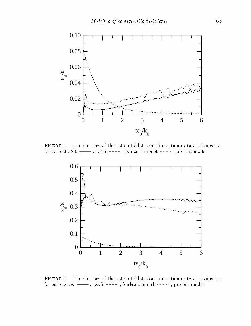
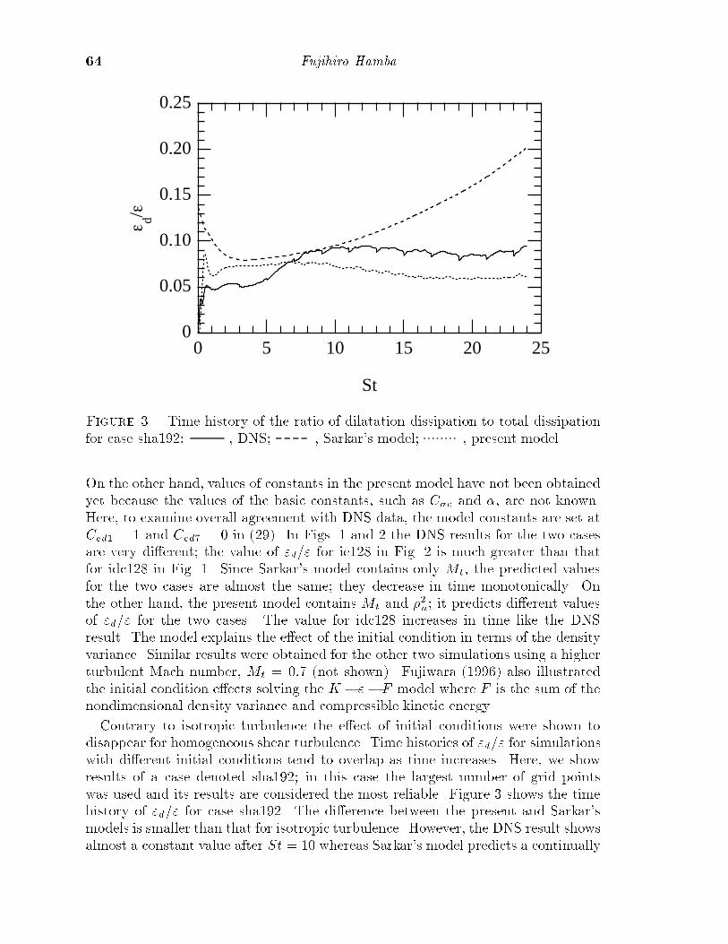
Figures � and show the time history of the ratio �d� for cases idc�� and ie��The initial values of Mt are the same for the two cases whereas those of �n and �care di�erent� The solid lines denote the DNS results� the dashed lines denote thevalues predicted by Sarkar�s model � � and the dotted lines denote those by thepresent model �� The model constant in Sarkar�s model is given by CedS � ��


0.10

0.08

0.06

0.04

0.02

0

ε d/ε

6543210

tε0/k

0

Figure �� Time history of the ratio of dilatation dissipation to total dissipationfor case idc�� DNS� � Sarkar�s model� � present model�

0.6

0.5

0.4

0.3

0.2

0.1

0

ε d/ε

6543210

tε0/k

0

Figure �� Time history of the ratio of dilatation dissipation to total dissipationfor case ie�� DNS� � Sarkar�s model� � present model�


0.25

0.20

0.15

0.10

0.05

0

ε d/ε

2520151050

St

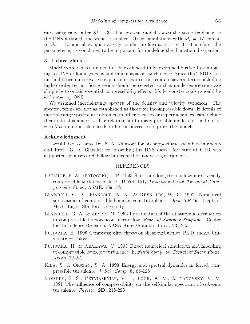
Figure �� Time history of the ratio of dilatation dissipation to total dissipationfor case sha�� DNS� � Sarkar�s model� � present model�

On the other hand� values of constants in the present model have not been obtainedyet because the values of the basic constants� such as C�c and �� are not known�Here� to examine overall agreement with DNS data� the model constants are set atCed� � � and Ced� � � in �� In Figs� � and the DNS results for the two casesare very di�erent� the value of �d� for ie�� in Fig� is much greater than thatfor idc�� in Fig� �� Since Sarkar�s model contains only Mt� the predicted valuesfor the two cases are almost the same� they decrease in time monotonically� Onthe other hand� the present model contains Mt and ��n� it predicts di�erent valuesof �d� for the two cases� The value for idc�� increases in time like the DNSresult� The model explains the e�ect of the initial condition in terms of the densityvariance� Similar results were obtained for the other two simulations using a higherturbulent Mach number� Mt � �� not shown� Fujiwara �� also illustratedthe initial condition e�ects solving the K � �� F model where F is the sum of thenondimensional density variance and compressible kinetic energy�

Contrary to isotropic turbulence the e�ect of initial conditions were shown todisappear for homogeneous shear turbulence� Time histories of �d� for simulationswith di�erent initial conditions tend to overlap as time increases� Here� we showresults of a case denoted sha�� in this case the largest number of grid pointswas used and its results are considered the most reliable� Figure shows the timehistory of �d� for case sha�� The di�erence between the present and Sarkar�smodels is smaller than that for isotropic turbulence� However� the DNS result showsalmost a constant value after St � �� whereas Sarkar�s model predicts a continually


increasing value after St � � The present model shows the same tendency asthe DNS although the value is smaller� Other simulations with Mt � �� extendto St � �� and show qualitatively similar pro�les as in Fig� � Therefore� theparameter �n is concluded to be important for modeling the dilatation dissipation�

�� Future plans

Model expressions obtained in this work need to be examined further by compar�ing to DNS of homogeneous and inhomogeneous turbulence� Since the TSDIA is amethod based on derivative expansions� expressions contain several terms includinghigher�order terms� Some terms should be selected so that model expressions aresimple but contain essential compressibility e�ects� Model constants also should beestimated by DNS�We assumed inertial�range spectra of the density and velocity variances� The

spectral forms are not as established as those for incompressible �ows� If details ofinertial�range spectra are obtained in other theories or experiments� we can includethem into this analysis� The relationship to incompressible models in the limit ofzero Mach number also needs to be considered to improve the models�

Acknowledgment

I would like to thank Dr� N� N� Mansour for his support and valuable commentsand Prof� G� A� Blaisdell for providing his DNS data� My stay at CTR wassupported by a research fellowship from the Japanese government�

REFERENCES

Bataille� F� � Bertoglio� J��P� �� Short and long term behaviour of weaklycompressible turbulence� In FED�Vol� �� Transitional and Turbulent Com�

pressible Flows� ASME� � ��

Blaisdell� G� A�� Mansour� N� N�� Reynolds� W� C� �� Numericalsimulations of compressible homogeneous turbulence� Rep� TF�� Dept� ofMech� Engr�� Stanford University�

Blaisdell� G� A� � Zeman� O� �� Investigation of the dilatational dissipationin compressible homogeneous shear �ow� Proc� of Summer Program� Centerfor Turbulence Research� NASA Ames�Stanford Univ��

Fujiwara� H� �� Compressibility e�ects on shear turbulence� Ph�D� thesis� Uni�versity of Tokyo�

Fujiwara� H� � Arakawa� C� �� Direct numerical simulation and modelingof compressible isotropic turbulence� In Ninth Symp� on Turbulent Shear Flows�Kyoto� ��

Kida� S� � Orszag� S� A� �� Energy and spectral dynamics in forced com�pressible turbulence� J� Sci� Comp� ��

Moiseev� S� S�� Petviashvily� V� I�� Toor� A� V�� Yanovsky� V� V�

�� The in�uence of compressibility on the selfsimilar spectrum of subsonicturbulence� Physica� �D� ��


Sarkar� S� �� The pressure�dilatation correlation in compressible �ows� Phys�Fluids A� ��

Sarkar� S� �� The stabilizing e�ect of compressibility in turbulent shear �ow�J� Fluid Mech� ��

Sarkar� S�� Erlebacher� G�� Hussaini� M� Y�� Kreiss� H� O� �� Theanalysis and modelling of dilatational terms in compressible turbulence� J� FluidMech� ��

Speziale� C� G� �� On nonlinear K � � and K � � models of turbulence� J�Fluid Mech� ��

Taulbee� D� � VanOsdol� J� �� Modeling turbulent compressible �ows� Themass �uctuating velocity and squared density� AIAA Paper� No� ��

Yoshizawa� A� �� Statistical analysis of the deviation of the Reynolds stressfrom its eddy�viscosity representation� Phys� Fluids� ��

Yoshizawa� A� �� Three�equationmodeling of inhomogeneous compressible tur�bulence based on a two�scale direct�interaction approximation� Phys� Fluids A��

Yoshizawa� A� �� Statistical analysis of compressible turbulent shear �ows withspecial emphasis on turbulence modeling� Phys� Rev� A� ��

Yoshizawa� A� �� Simpli�ed statistical approach to complex turbulent �owsand ensemble�mean compressible turbulence modeling� Phys� Fluids� ��

Yoshizawa� A� � Nisizima� S� �� A nonequilibrium representation of the tur�bulent viscosity based on a two�scale turbulence theory� Phys� Fluids A� ��

��

Zeman� O� �� Dilatation dissipation� The concept and application in modelingcompressible mixing layers� Phys� Fluids A� ��

Zeman� O� �� On the decay of compressible isotropic turbulence� Phys� FluidsA� ��

by ujihiro ham ba

Documents